the Creative Commons Attribution 4.0 License.
the Creative Commons Attribution 4.0 License.
 | 15 Nov 2023
Characterizing the tropospheric water vapor spatial variation and trend using 2007–2018 COSMIC radio occultation and ECMWF reanalysis data
Xi Shao
Shu-Peng Ho
Xin Jing
Xinjia Zhou
Yong Chen
Tung-Chang Liu
Bin Zhang
Jun Dong
Atmospheric water vapor plays a crucial role in the global energy balance, hydrological cycle, and climate system. High-quality and consistent water vapor data from different sources are vital for weather prediction and climate research. This study assesses the consistency between the Formosa Satellite Mission 3–Constellation Observing System for Meteorology, Ionosphere, and Climate (FORMOSAT-3/COSMIC) radio occultation (RO) and European Centre for Medium-Range Weather Forecasts (ECMWF) Reanalysis Model 5 (ERA5) water vapor datasets. Comparisons are made across different atmospheric pressure levels (300, 500, and 850 hPa) from 2007 to 2018. Generally, the two datasets show good spatial and temporal agreement. COSMIC's global water vapor retrieval is slightly lower than ERA5's at 500 and 850 hPa, with distinct latitudinal differences between hemispheres. COSMIC exhibits global water vapor increasing trends of 3.47 ± 1.77 % per decade, 3.25 ± 1.25 % per decade, and 2.03 ± 0.65 % per decade at 300, 500, and 850 hPa, respectively. Significant regional variability in water vapor trends, encompassing notable increasing and decreasing patterns, is observable in tropical and subtropical regions. At 500 and 850 hPa, strong water vapor increasing trends are noted in the equatorial Pacific Ocean and the Laccadive Sea, while decreasing trends are evident in the Indo-Pacific Ocean region and the Arabian Sea. Over land, substantial increasing trends at 850 hPa are observed in the southern United States, contrasting with decreasing trends in southern Africa and Australia. The differences between the water vapor trends of COSMIC and ERA5 are primarily negative in the tropical regions at 850 hPa. However, the water vapor increasing trends at 850 hPa estimated from COSMIC are significantly higher than the ones derived from ERA5 data for two low-height stratocumulus-cloud-rich ocean regions west of Africa and South America. These regions with notable water vapor trend differences are located in the Intertropical Convergence Zone (ITCZ) area with frequent occurrences of convection, such as deep clouds. The difference in characterizing water vapor distribution between RO and ERA5 in deep cloud regions may cause such trend differences. The assessment of spatiotemporal variability in RO-derived water vapor and reanalysis of atmospheric water vapor data helps ensure the quality of these datasets for climate studies.
- Article
(10835 KB) - Full-text XML
- BibTeX
- EndNote


Water vapor is one of the most important greenhouse gases in the atmosphere, which accounts for about 60 % of the natural greenhouse effect (Kiehl and Trenberth, 1997; Wagner et al., 2006; Foster et al., 2007; Ahrens and Samson, 2011). Water vapor cycles with latent heat release through condensation and evaporation are closely linked to cloud formation, which alters atmospheric energy budgets. In addition, studies showed that water vapor amplifies global warming (Smith and Reynolds, 2005; Parker et al., 2007; Dai, 2006; Allan and Soden, 2008; Mieruch et al., 2008; Zhang et al., 2013). As the Earth warms, the water vapor concentration in the lower troposphere increases with increasing temperature, increasing the evaporation rate and adding more atmospheric water vapor, which usually warms the atmosphere further. Water vapor's heat-trapping effect is crucial in climate change (Forster et al., 2007). Studies (i.e., Foster et al., 2007; Allan and Liepert, 2010; Trenberth, 2011; Hegerl et al., 2015) show that water vapor has profound impacts on atmospheric temperature structure and the hydrological cycle, which, in turn, increases the likelihood of extreme regional precipitation events, extreme weather conditions, and droughts.
Accurate atmospheric water vapor climate data records (CDRs) are critical for detecting climate change. Various studies have quantified the spatial and temporal variation and trend in atmospheric water vapor using two types of water vapor data: (i) measurements or retrievals from sensor observations and (ii) reanalysis data produced by assimilating various observations. The first data type includes both ground-based in situ and spaceborne observations: long-term radiosonde measurements (Zhai and Eskridge, 1997; Ross and Elliott, 2001; Ho et al., 2010; Zhao et al., 2012; Zhang et al., 2018), weather station data (Dai, 2006), water vapor retrieved from ground-based Global Positioning System (GPS) station data (Kursinski et al., 1997; Bock et al., 2007; Nilsson and Elgered, 2008; Vey et al., 2010; Huang et al., 2013; Chen and Liu, 2016; Yuan et al., 2023), water vapor retrievals from spaceborne radio occultation observations (Ho et al., 2009; Huang et al., 2013, 2018; Zhang et al., 2018; Andrisaniand and Vespe, 2020; Gleisner et al., 2022), visible-spectral-range sensor observations (Mieruch et al. 2008; Grossi et al., 2015; Borger et al., 2023), microwave observations (Rosenkranz, 2001; Chen and Liu, 2016; Ho et al., 2018; Yadav et al., 2021), and infrared sounder observations (Susskind et al., 2003).
The second type of water vapor data are from the global atmospheric reanalysis products generated by the European Centre for Medium-Range Weather Forecasts (ECMWF) (Hersbach et al., 2020) and the National Centers for Environmental Prediction (NCEP) (Whitaker et al., 2008). These reanalysis data are constructed from assimilating in situ and satellite observations through data assimilation (DA) systems blended with model outputs. These atmospheric reanalysis data have been used for investigating long-term atmospheric water vapor variability and trends (Bengtsson, 2004; Wagner et al., 2006; Adler et al., 2008; Ho et al., 2009; Huang et al., 2013; Zhang et al., 2013; Chen and Liu, 2016; Xie et al., 2020; He et al., 2022) as well as climate change studies (Allan, 2002; Allan et al., 2014; Lu et al., 2015). However, the quality of the reanalysis data may be affected by (i) discontinuity or changes of in situ data and satellite data, (ii) the inadequate spatial and temporal coverage of the observations, (iii) inadequate measurement bias corrections, (iv) preliminary observation error estimates, (v) contamination of ground-based and spaceborne satellite observations due to clouds, and (vi) potential and/or unknown model errors (Sherwood et al., 2010; Chen and Liu, 2016). The uncertainty of forecast and reanalysis data under cloudy conditions, especially over oceans, is still very large (Lonitz and Geer 2017).
Past climate modeling studies suggest that increasing surface temperature can result in an increasing trend in global water vapor (Held and Soden, 2000, 2006; Santer et al., 2006). Studies based on various types of observations and reanalysis data have shown an increasing water vapor trend over different periods ranging from several decades to the recent decade (Bengtsson, 2004; Wagner et al., 2006; Ho et al., 2009; Chen and Liu, 2016; Wang et al., 2017; Ho et al., 2018). However, these studies also showed substantial variation (with both increasing and decreasing) in regional water vapor trends (Ross and Elliott, 2001; Dai, 2006; Mieruch et al., 2008, 2014; Zhang et al., 2018). This is mainly because regional water vapor concentration may change dramatically depending on multiple non-thermodynamic factors such as (i) surface type, (ii) long-range transport of air masses, and (iii) water availability. As a result, the global surface temperature increase does not increase water vapor everywhere (Chou and Neelin, 2004; Wagner et al., 2006; Lu et al., 2015; Chen and Liu, 2016).
Many studies (i.e., Ho et al., 2009; Chen and Liu, 2016; Ho et al., 2018) have compared global reanalysis of water vapor with those derived from in situ and satellite sensors. For example, Chen and Liu (2016) evaluated the global precipitable water vapor (PWV) variability and trend from ECMWF and NCEP reanalysis results. They compared the water vapor reanalysis with 36-year (1979 to 2014) water vapor datasets collected from radiosonde, ground-based Global Navigation Satellite System (GNSS), and microwave satellite observations. All these datasets showed increasing PWV trends. The ERA-Interim reanalysis agrees with microwave satellite observations better than those from the NCEP reanalysis. ERA-Interim overestimates the PWV over the ocean for the period before 1992 compared to microwave satellite data. It is essential to continue comparing the differences and consistencies of atmospheric water vapor data's temporal and spatial variabilities from different sources and provide the climate community with high-quality water vapor data.
There is growing interest in comparing reanalysis data and all-weather water vapor profiles retrieved from GNSS radio occultation (RO) (Anthes et al., 2020; Kursinski and Hajj, 2021; Ho et al., 2009, 2010; Johnston et al., 2022). Complementing the measurements from microwave and infrared sounders, RO data can provide information on the temperature, water vapor, and pressure with high accuracy, precision, and vertical resolution. Because the quality of RO data does not change during the day or night and is not affected by clouds (Anthes et al., 2008; Ho et al. 2020a), the RO temperature and water vapor profiles collocated with reanalysis data would help identify the variation of temperature and humidity under all weather conditions over time. RO data have been used to evaluate biases and monitor calibration changes for microwave measurements (Iacovazzi et al., 2020; Shao et al., 2021a) and infrared sounders (Chen et al., 2022). Further, RO-derived water vapor profiles have been used to distinguish systematic water vapor biases in radiosondes (Ho et al., 2010; Sun et al., 2019; Ho et al., 2020a; Shao et al., 2021b).
In this paper, we characterize the water vapor data derived from the Formosa Satellite Mission 3–Constellation Observing System for Meteorology, Ionosphere, and Climate (FORMOSAT-3/COSMIC) (hereafter COSMIC) and those from ECMWF Reanalysis Model 5 (ERA5). Launched in 2006, COSMIC was the first constellation of microsatellites carrying GPS RO receivers. COSMIC has demonstrated the value of RO data in the ionosphere for climate and meteorological research as well as operational weather forecasting (Ho et al., 2020a). This paper aims to characterize and compare the global, latitudinal, and regional variabilities of COSMIC and ERA5 water vapor distributions, seasonality, and long-term trends at selected pressure levels from 2007 to 2018. In addition, this paper identifies regions with notable increasing and decreasing water vapor trends, i.e., regions becoming moister or drier, and regions with significant water vapor trend differences between COSMIC and ERA5. Particular emphasis is also placed on comparing the COSMIC and ERA5 water vapor trends over stratocumulus-cloud-rich regions to investigate the impacts of stratocumulus clouds on near-surface water vapor data quality in ERA5.
This paper is organized as follows: Sect. 2 introduces the water vapor data from COSMIC RO retrieval and ERA5 reanalysis. Section 3 analyzes global and latitudinal variabilities of long-term (2007–2018) COSMIC and ERA5 water vapor data at three pressure levels, and their differences are quantified. In Sect. 4, the global and latitudinal water vapor trends derived from COSMIC and ERA5 are quantified and compared at different pressure levels. Section 5 examines the overall distribution of regional water vapor trends derived from the COSMIC and ERA5 time series and their differences. Furthermore, a few specific sites with frequent stratocumulus cloud coverage and large differences between COSMIC and ERA5 are selected to quantify the water vapor trend differences. Additionally, the seasonal variability of latitudinal water vapor distribution is summarized in Appendix A1. Appendix A2 and A3 describe the estimation of the water vapor trend with sampling error removal and its associated uncertainties for a given region of interest (RoI). Appendix A4 provides additional information on a few sites with notable increasing and decreasing water vapor trends. We present the conclusions and discussion in Sect. 6.
2.1 ECMWF reanalysis data
This study used the ERA5 global atmospheric and climate reanalysis dataset (https://www.ecmwf.int/en/forecasts/dataset/ecmwf-reanalysis-v5, last access: 7 November 2023). ERA5 is the fifth-generation ECMWF reanalysis dataset covering the past 4 to 7 decades. The ERA5 dataset is generated from the four-dimensional variational (4D-Var) data assimilation system, which uses a fixed version of the ECMWF NWP system, i.e., Integrated Forecasting System (IFS) Cy41r2. The IFS Cy41r2 system became operational in 2016 (Hersbach et al., 2020) and blends or assimilates meteorological observations (e.g., surface weather stations, ocean buoys, radiosonde stations, aircraft, and remote sensing satellites) with a previous forecast to obtain the best for both. These blended results serve as the initial conditions for the next forecast period. The ERA5 water vapor data are from the ground to ∼ 0.1 hPa at 37 mandatory pressure levels. Our study used ERA5 global water vapor profiles from 2007 to 2018 in 6 h increments. The ERA5 data were collected with a 0.25∘ spatially gridded resolution, equivalent to a spatial resolution of ∼ 25 km at the Equator. Many studies have been conducted to validate the ERA5 atmospheric products using satellite measurements (Chen and Liu, 2016; Lei et al., 2020; Tang et al., 2021; Campos et al., 2022). Overall, the results of these studies show that ERA5 is in good agreement with satellite measurements (or retrieved products). For example, Tang et al. (2021) compared the atmospheric downward longwave radiation (DLR) from Clouds and Earth's Radiant Energy System (CERES) satellite retrievals and ERA5 data with observations at Baseline Surface Radiation Network (BSRN) stations over land surfaces. The ERA5 atmospheric reanalysis performed better than satellite retrievals in estimating DLR over the land surface. According to Chen and Liu (2016), the global water vapor trend over 1992–2014 from the data of the ECMWF reanalysis model agrees well with the microwave satellite data. These studies provide confidence in the accuracy of the ERA5 products for comparison with COSMIC retrievals.
2.2 COSMIC WETPrf water vapor retrieval
The COSMIC RO receivers on low-Earth orbit (LEO) satellites measure the phase delay of radio waves, which are emitted from GPS satellites and bent by atmospheric refraction. Profiles of atmospheric refractivity can be derived from the bending angles of radio wave trajectories when propagating through the ionosphere, stratosphere, and troposphere. From the retrievals of RO limb-sounding observations, the bending angle and refractivity profiles from the excess phase data processed from the Doppler-shifted raw radio signals transmitted by GPS satellites are derived. Then, the one-dimensional variational (1D-Var) retrieval algorithm is applied to solve an under-determined problem: determine the atmospheric temperature and water vapor profiles from bending angle or refractivity data. The 1D-Var retrieval generally uses the a priori state of the atmosphere, i.e., vertical background temperature and humidity profiles, and associated background and observation uncertainties as well as error covariance matrices (ECMs) to minimize a quadratic cost function.
In this paper, we analyze the 2007 to 2018 COSMIC wet profile data produced by the University Corporation for Atmospheric Research (UCAR) from COSMIC RO data, namely WETPrf (https://cdaac-www.cosmic.ucar.edu/cdaac/products.html, last access: 7 November 2023). The WETPrf data from the COSMIC Data Analysis and Archive Center (CDAAC) consist of temperature, water vapor, and pressure profiles with a high vertical resolution (100 m). UCAR WETPrf profile data contain the latitude and longitude of the RO perigee point, temperature, pressure, water vapor profile, and mean sea level height. COSMIC has provided more than 7 million RO sounding profiles over its lifetime. Many of the six COSMIC GPS receivers continued beyond their 2-year designed life and provided more than 1000 occultation profiles per day through 2016. The COSMIC data decreased significantly in late 2019 and was decommissioned in May 2020.
The UCAR COSMIC WETPrf data were generated with the heritage 1D-Var algorithm at CDAAC to produce wet temperature and humidity profile data. In the 1D-Var algorithm for WETPrf, background profiles are taken from ERA-Interim gridded low-resolution data and interpolated to the time and location of RO measurements to separate the pressure, temperature, and moisture contributions to the refractivity. The constraint applied to WETPrf in the 1D-Var retrieval is very tight such that temperature and moisture profiles are reported only when the residual refractivity (i.e., the difference between the observed refractivity and simulated refractivity computed from the retrieved temperature and moisture profiles) is within the uncertainty of refractivity. This ensures that the information on refractivity measurements from RO is completely used in the 1D-Var (Ho et al., 2020a).
2.3 Method of comparing COSMIC and ERA5 water vapor data
In our analysis, COSMIC RO profiles with the “bad” flag have been filtered out. COSMIC RO and ERA5 water vapor profiles were paired through collocation before the analysis was performed. The ERA5 data have a global distribution over 0.25∘ latitude–longitude grids, vertically over 37 pressure layers, and at 6 h intervals. Therefore, the ERA5 water vapor data at a given pressure level are interpolated at the latitude–longitude of the perigee point of the RO profile and at RO time to match the COSMIC RO measurement. For the RO data, the fine-vertical-resolution COSMIC RO water vapor profiles are interpolated onto three pressure levels, e.g., 300, 500, and 850 hPa, selected to characterize water vapor variations at representative altitudes around 9, 5.5, and 1.5 km, respectively.
The pressure level at 850 hPa studied in this paper is close to the surface and within the boundary layer. Its water vapor can vary based on factors such as humidity levels near the surface, regional water vapor sources, and weather patterns. From previous studies (Ho et al., 2009, 2020a; Shao et al., 2021a; Johnston et al., 2021) of comparing RO water vapor data with collocated reanalysis model data or radiosonde measurements, it was found that RO water vapor retrievals have a negative bias in the lower troposphere. The COSMIC water vapor retrieval is strongly affected by super-refraction at this pressure level in moisture-rich regions (Ho et al., 2010). It is worth evaluating the relative biases and consistency in the trends on various spatial scales between COSMIC and ERA5 water vapor datasets at this 850 hPa pressure level.
The water vapor at 500 hPa can vary widely depending on local weather conditions and atmospheric patterns. Water vapor at 500 hPa is crucial for understanding the development of weather patterns, including midlatitude cyclones, ridges, and troughs. This pressure level also contributes to the upper-level atmospheric circulation patterns through convection, which carries moist air upward from the lower troposphere and plays a role in redistributing heat and moisture. It was learned from the earlier comparison of RO data with radiosonde measurements that starting from the pressure level at 500 hPa, the RO water vapor retrieval uncertainty increases as altitude decreases. Therefore, we chose 500 hPa as the representative middle troposphere of interest to study in this paper.
The 300 hPa pressure level represents the water vapor layer with fewer horizontal variations at higher altitudes. Water vapor in the upper troposphere plays a critical role in the Earth's radiative balance and climate system. It affects the absorption and emission of radiation, contributing to warming (absorbing and trapping infrared radiation, i.e., the greenhouse effect) and cooling (emitting heat energy) effects. Johnston et al. (2021) showed large discrepancies in the ERA5 and MERRA2 reanalysis model water vapor profiles compared to COSMIC-2 in the upper troposphere. There are large uncertainties for the reanalysis model to estimate the upper troposphere water vapor due to the combined effects of complex atmospheric dynamics (jet streams, convection, and mixing) at high altitudes, sparse observations, difficulties in validation, errors in extrapolating from lower-altitude measurements, and accurate accounting of radiative effects at high altitudes. Therefore, we chose 300 hPa as the representative upper troposphere level to compare spatial and temporal variabilities of water vapor between COSMIC and ERA5.
2.4 Impact of ERA-Interim as a priori on COSMIC water vapor retrieval
The UCAR's 1D-Var retrieval algorithm for COSMIC WETPrf (water vapor and humidity) uses ERA-Interim profiles as the a priori input (Wee et al., 2022). In addition, the UCAR WETPrf water vapor and temperature retrieval also enforces a retrieval constraint to the residual refractivity. Such a constraint can determine the influence of ERA-Interim on the final water vapor retrieval at different pressure levels. On the other hand, ERA5 provides a more comprehensive and reliable reanalysis by using improved weather forecast and data assimilation models with various ground, in situ, and satellite measurements compared to ERA-Interim (Fujiwara et al., 2017; Hersbach et al., 2020). Figure 1 depicts the monthly (using January and July of 2007 as representative winter and summer months of the Northern Hemisphere) scatter plots of the collocated COSMIC global water vapor versus ERA5 and ERA-Interim water vapor data at three pressure levels. The linear regression statistics for COSMIC versus ERA5 and COSMIC versus ERA-Interim comparisons are also shown on the plots. All plots show that COSMIC versus ERA-Interim comparisons are more scattered than the COSMIC versus ERA5 comparison. Quantitatively, the correlation coefficients between COSMIC and ERA5 are around 0.96, while the correlation coefficient between COSMIC and ERA-Interim varies from 0.88 to 0.93. The linear fitting coefficients, i.e., slopes, of COSMIC versus ERA5 fittings are closer to 1 than COSMIC versus ERA-Interim fitting in all panels of Fig. 1. In terms of the linear fitting root mean square error (RMSE) residuals, the RMSEs of COSMIC versus ERA5 fitting are lower than the COSMIC versus ERA-Interim fitting by 24 % to 47 % over the two selected months (January and July of 2007) and three pressure levels. These analysis results indicate that the COSMIC water vapor retrievals are more consistent with ERA5 than ERA-Interim. It suggests that the information on COSMIC 1D-Var retrievals is mainly from the COSMIC refractivity instead of the ERA-Interim. We also inspected the comparison of COSMIC versus ERA5 or ERA-Interim for other months (not shown here), and the conclusion that COSMIC water vapor data are more consistent with ERA-5 than ERA-Interim holds for these months as well.
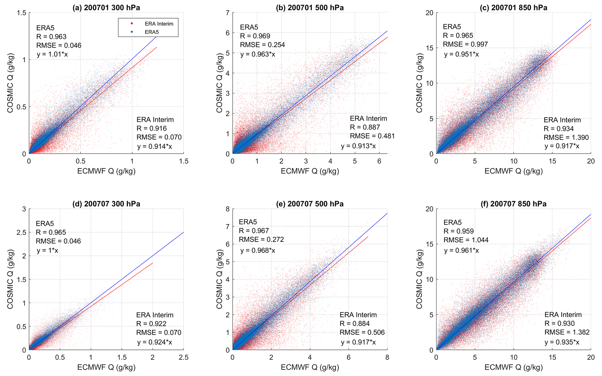
Figure 1Scatter plots of collocated COSMIC water vapor retrieval versus ERA5 and ERA-Interim water vapor data for 2 months (a, b, c: January 2007; d, e, f: July 2007) at three pressure levels: (a, d) 350 hPa, (b, e) 500 hPa, and (c, f) 850 hPa. The correlation coefficient (R), linear fitting coefficient, and RMSE of the fitting residual for COSMIC water vapor retrieval versus ERA5 and ERA-Interim comparisons are listed in each panel.
The comparisons between COSMIC and ERA5 water vapor (Fig. 1) suggest overall consistencies over the two selected months and at three pressure levels, which requires further quantitative analysis of the variabilities. In the following sections, we analyze the collocated COSMIC and ERA5 water vapor at three pressure levels to study their spatial (Sect. 3) and trend (Sects. 4 and 5) variabilities (the seasonal trend is provided in Appendix A1).
3.1 Global distribution of COSMIC and ERA5 water vapor
To intercompare the spatial variability of the water vapor data between COSMIC and ERA5 (interpolated onto COSMIC locations and times), the collocated global humidity data over 12 years (2007–2018) are grouped into 10∘ × 10∘ latitude–longitude grids and spatial- and time-averaged at three selected pressure levels, e.g., 300, 500, and 850 hPa.
Figure 2 compares time-averaged global water vapor distribution maps over three pressure levels between COSMIC (left column) and ERA5 (right column). The overall global distribution of water vapor of COSMIC and ERA5 at three pressure levels is generally consistent. At all three pressure levels, the global water vapor distribution exhibits a high concentration in the low-latitude tropical regions, decreases rapidly toward the polar region, and is low in some high-terrain regions such as the Tibetan Plateau. In the low-latitude tropical region, i.e., latitudes between −20 and 20∘, increased water vapor concentrations occur in the eastern Indian and western Pacific Ocean regions and over the Amazon rainforest regions in South America at these three pressure levels. It is noted that COSMIC bending angles are assimilated into ERA5, which significantly improves the upper troposphere and lower stratosphere temperatures (Hersbach et al., 2020). However, the COSMIC 1D-Var retrieval has more independence from its a priori (ERA-Interim) for water vapor within the lower–middle troposphere. Primary water vapor information is retrieved from the RO observations at these altitudes, which our study is focused on. The evaluations of global and latitude-dependent water vapor differences between COSMIC and ERA5 in the following sections would help understand the extent and regional dependence of the assimilation of COSMIC RO water vapor data in ERA5.
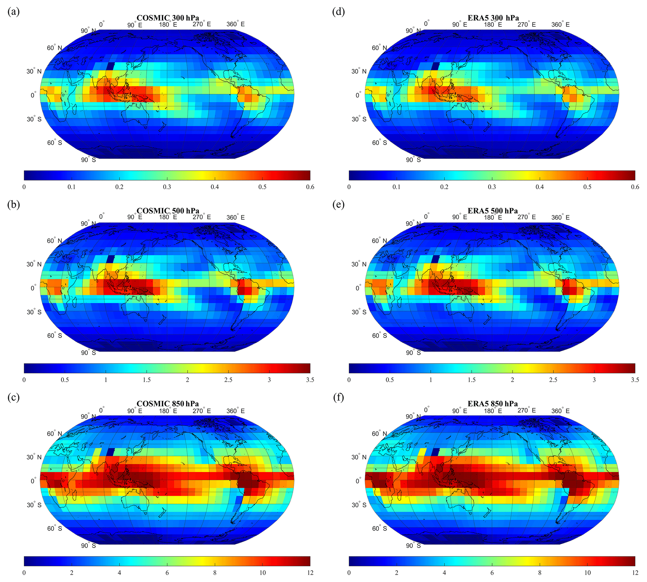
Figure 2Comparison of the global distribution of 10×10∘ grid-averaged water vapor (g kg−1) data between COSMIC retrievals (a, b, c) at 300, 500, and 850 hPa and ERA5 data (d, e, f) at 300, 500, and 850 hPa, respectively.
To quantitatively evaluate the consistency between COSMIC and ERA5 water vapor (Q) data, the relative biases (%) between COSMIC and ERA5 are calculated with the 12-year collocated COSMIC and ERA5 global water vapor data. The mean differences between COSMIC and ERA5 global water vapor are 5.67 ± 34.30 %, −1.86 ± 30.09 %, and −2.30 ± 21.21 % for pressure levels at 300, 500, and 850 hPa, respectively. This suggests that at 500 and 850 hPa, COSMIC water vapor retrieval is lower than ERA5 water vapor data. This is consistent with the negative moisture biases below 5 km for the RO retrievals compared to the collocated radiosonde data (Ho et al., 2009, 2020a; Shao et al., 2021b). Such near-surface moisture biases may come from the 1D-Var RO retrieval when super-refraction with a sharp refractivity gradient occurs in the moisture-rich low-tropospheric RO profiles (Ho et al., 2020b; Shao et al., 2021a, b). At 300 hPa, the COSMIC water vapor concentration is about 5.67 % higher than ERA5. Since the water vapor concentration at 300 hPa is very low, its contribution to the total precipitable water would be minimal. The fact that at 300 hPa water vapor from COSMIC is higher than from ERA5 stems from the distinctive cloud penetration capability of the RO signal. In contrast, there are uncertainties in the water vapor from the reanalysis data over the cloud-free scenes since these scenes can be over thin or cirrus clouds due to the difficulty of data assimilation over these types of clouds. The water vapor concentration derived from COSMIC is expected to be higher than ERA5 at 300 hPa when thin or cirrus clouds are present. Our evaluation of water vapor at 300 hPa indicates that the difference between RO and ERA5 of about 5.7 % is likely due to the uncertainty in classifying cloud-free scenes in the data assimilation and in the RO retrieval system. Such assessment is consistent with the water vapor biases between COSMIC-2 and ERA5 presented in Johnston et al. (2021).
We also notice significant uncertainties in estimating upper troposphere water vapor in the reanalysis model. Johnston et al. (2021) analyzed COSMIC-2 and reanalysis (ERA5 and MERRA2) water vapor differences in different latitude zones. It was shown that the UCAR COSMIC-2 water vapor retrieval is consistently lower than both ERA5 and MERRA2 water vapor data in the lower troposphere (below 2 km). However, COSMIC-2 water vapor retrieval data are higher than ERA5 data and lower than MERRA2 data at altitudes above 5 km. The magnitude of the COSMIC-2 vs. ERA5 water vapor difference is smaller than that of COSMIC-2 vs. MERRA2 above 5 km. The opposite sign and large magnitude of the ERA5 and MERRA2 model water vapor differences relative to COSMIC-2 in the upper troposphere suggest large uncertainties in calculating water vapor in the reanalysis model over this altitude region. There are ongoing efforts to quantify the ERA5 biases in the upper troposphere through comparison with other measurements, such as using multi-campaign datasets from research aircraft (Krüger et al., 2022). However, the results are inconclusive due to the comparison's limited regional, height, and temporal coverage. In this regard, the comparisons presented in this paper help assess the biases in the reanalysis model. Further comparisons with collocated radiosonde measurements can also help assess the biases in ERA5 in the upper troposphere.
3.2 Latitude dependence of COSMIC and ERA5 water vapor distribution
The comparisons of the latitudinal dependence of water vapor distribution between COSMIC and ERA5 at three pressure levels are shown in Fig. 3. Eight latitudinal bins from −80 to 80∘ with 20∘ bin width are used to group COSMIC and ERA5 water vapor data. The 20∘ wide latitude bins over the Northern and Southern Hemisphere are selected to characterize water vapor latitude dependence in different reprehensive latitudinal zones such as 0–20∘ for tropical, 20–40∘ for subtropical, 40–60∘ for midlatitude, and 60–80∘ for high-latitude regions. The regions with latitudes above 80∘ were not selected due to much less data coverage from COSMIC. The collocated COSMIC and ERA5 water vapor data over all months in 12 years (2007–2018) have been used to calculate the mean water vapor over these latitude bins, as shown in Fig. 3. Figure 3a, d, and g show the side-by-side comparison of COSMIC and ERA5 water vapor data averaged over 20∘ latitude bins at the three selected pressure levels (300, 500, and 850 hPa), respectively. The panels in the middle and right columns of Fig. 3 show the latitude dependence of the COSMIC minus ERA5 water vapor mean difference ( and relative difference (.
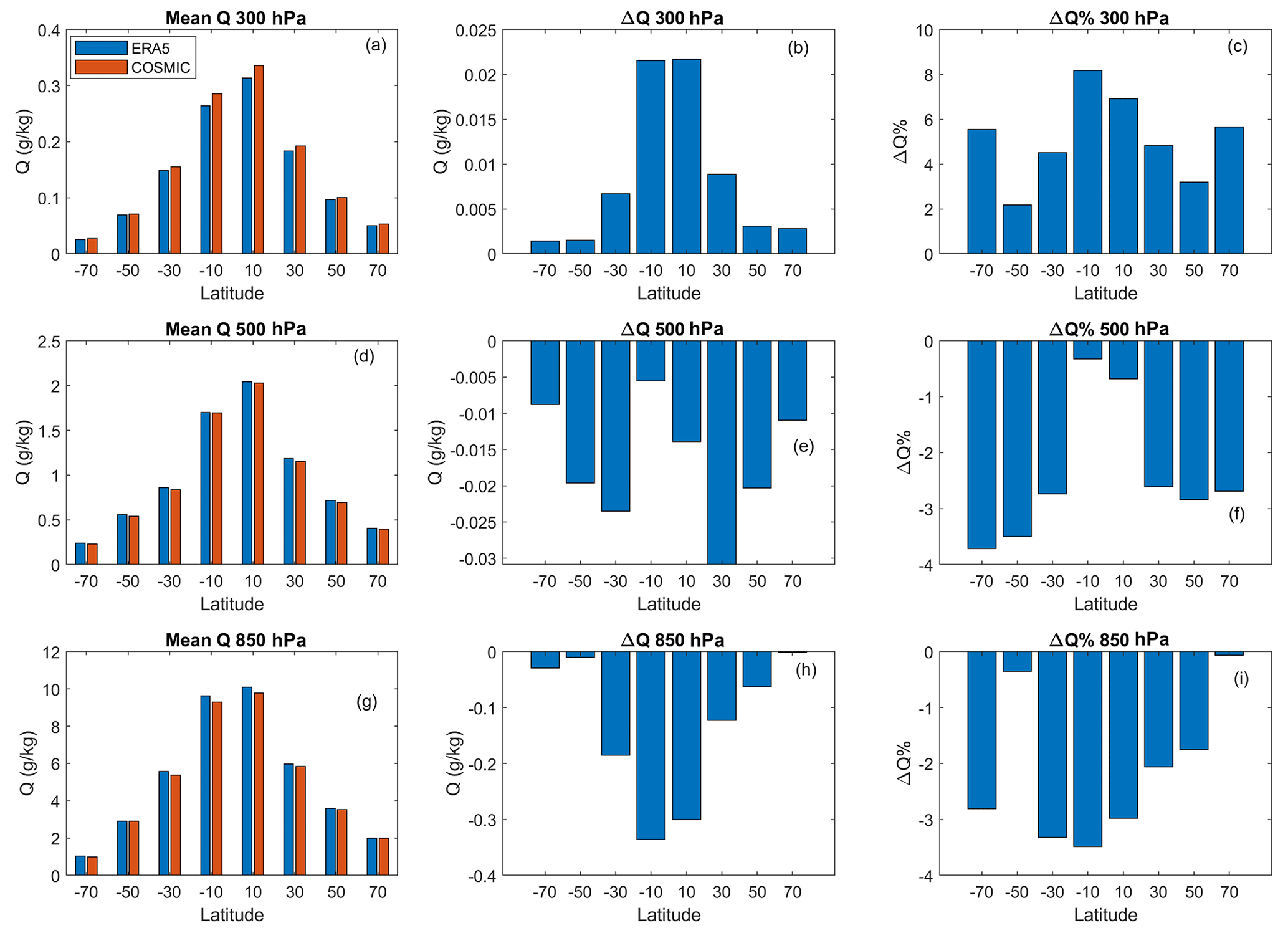
Figure 3(a, d, g) Comparison of bin-mean water vapor between COSMIC-retrieved data and ERA5 data at three pressure levels. Panels (b), (e), and (h) as well as (c), (f), and (i) show the value difference and percent difference (COSMIC minus ERA5) of latitude-bin-mean water vapor data between COSMIC-retrieved data and ERA5 data, respectively. The top, middle, and bottom rows show the comparisons at 300, 500, and 850 hPa, respectively. In all bar chart panels, the bar centers on the x axis are placed at the centers of the 20∘ latitudinal bins. For this figure, collocated COSMIC and ERA5 water vapor data for all months of the considered 12-year period (2007–2018) have been used to calculate the mean water vapor in the corresponding latitude bins.
In general, COSMIC and ERA5 water vapor data (Fig. 3) show that latitudinal water vapor distribution peaks in the −20 to 20∘ equatorial latitude zones and rapidly decreases toward the polar region at all three pressure levels. There is an asymmetry in the latitude-dependent distribution of water vapor between the Northern and Southern Hemisphere. For example, the Northern Hemisphere's 0 to 20∘ Equator latitude bin has the highest water vapor compared with all other latitude bins, including the southern −20 to 0∘ latitude bin for all three pressure levels. The decrease in water vapor from the low-latitude tropics to the polar region in the Southern Hemisphere is more rapid than in the Northern Hemisphere, which results in a higher water vapor concentration in the northern latitudinal bins than the corresponding latitudinal bins in the Southern Hemisphere.
Feulner et al. (2013) showed the asymmetric distribution of annually and zonally averaged surface air temperatures between the Northern and Southern Hemisphere, with the mean surface air temperature in the Northern Hemisphere being 1–2 ∘C warmer than in the Southern Hemisphere. The close relationship between temperature and the capacity of the atmosphere to hold water vapor is governed by the Clausius–Clapeyron equation (Held and Soden, 2006). The equation states that for every 1 ∘C increase in temperature, the saturation vapor pressure increases by about 7 %. As temperature increases, this will lead to the potential for more water vapor to be held in the air. In other words, warmer air has a higher capacity to hold water vapor. This relationship is crucial for understanding how temperature changes can impact atmospheric humidity. The observed and modeled evidence presented by Wentz and Schabel (2000), Trenberth et al. (2005), Held and Soden (2006), and Allan et al. (2014) supports the notion that higher atmospheric water vapor contents are, in general, associated with higher temperatures.
Since warmer temperature is closely coupled with a higher water vapor evaporation rate, our findings of moister high-latitude zones in the Northern Hemisphere are consistent with the interhemispheric temperature difference observed in Feulner et al. (2013). Furthermore, Feulner et al. (2013) examined climatological data, Earth's energy budget, and model simulations for factors that could lead to interhemispheric temperature differences. The study of Feulner et al. (2013) compared various factors, including seasonal differences in solar radiation, the tropical land area difference, the difference in albedo and temperature between Antarctic and Arctic polar regions, and cross-equatorial ocean heat transport from the Southern Hemisphere to the Northern Hemisphere. It was shown by Feulner et al. (2013) that for the preindustrial climate, the northward meridional heat transport by ocean circulation, with an additional contribution from the albedo differences between the northern and southern polar regions, is the dominant factor for the interhemispheric temperature difference. As greenhouse gas emissions continued to rise throughout the industrial era, interhemispheric temperature disparities became larger. This is attributed to the intensified warming of land areas compared to oceans and the significant reduction of Arctic sea ice and snow cover in the Northern Hemisphere. These factors, including cross-equatorial ocean heat transport, albedo difference in polar regions, intensified warming of land areas, and reduction of Arctic ice–snow cover, which affect interhemispheric temperature difference, can also be the primary driving factors of the interhemispheric water vapor difference.
The comparisons between COSMIC and ERA5 water vapor at three pressure levels in the middle and right columns of Fig. 3 show some latitude-dependent differences. At the 300 hPa pressure layer, the mean difference and relative difference ΔQCOSMIC−ERA5 (%) are positive (Fig. 3b and c); i.e., QCOSMIC is higher than QERA5. The peak relative differences (∼ 7 %–8 %) occur in the two equatorial latitude bins (−20 to 0 and 0 to 20∘ bins). The percent difference values range from 2 % to 8 % over the eight latitudinal bins. This suggests that the 5.67 % bias in the global QCOSMIC versus QERA5 comparison mainly comes from the water vapor difference near the Equator.
At the 500 hPa pressure level, ΔQCOSMIC−ERA5 values (Fig. 3e) are negative for all the latitude bins, with the amplitude of the water vapor difference being low in the equatorial latitude bins, which is different from those at 300 hPa (Fig. 3b) and 850 hPa (Fig. 3h). At this pressure layer, the mean QCOSMIC is entirely consistent with the mean QERA5, i.e., ΔQCOSMIC−ERA5 (%) is within −0.5 % as shown in Fig. 3f, in the −20 to 20∘ latitude bins around the Equator. Away from the Equator, the percent difference ΔQCOSMIC−ERA5 (%) increases to around −3 %.
At the 850 hPa near-surface level, a consistent latitudinal pattern is evident (Fig. 3h and j), characterized by negative biases in ΔQCOSMIC−ERA5 across all eight latitude bins under investigation. From Fig. 3h, it can be seen that the amplitudes of negative ΔQCOSMIC−ERA5 are dominantly distributed over the −40 to 40∘ latitude zone while peaking at the −20 to 20∘ Equator zone, which agrees with the occurrence of negative water vapor bias in the COSMIC 1D-Var retrieval due to super-refraction in the near-surface moisture-rich low-latitude regions (Ho et al., 2010). From Fig. 3i it can be seen that ΔQCOSMIC−ERA5 values (% ) of all latitude bins have negative differences around −2 % to −3 % except for two latitude bins (−60 to −40∘ and 60 to 80∘) which have smaller negative ΔQCOSMIC−ERA5 (%) near zero.
With six satellites, COSMIC occultations generally have uniform spatial and temporal distributions. However, because the daily sample number of COSMIC occultations decreased dramatically after 2010 (see Fig. A4e in the Appendix), we need to remove the COSMIC sampling uncertainty for the trend calculation. A detailed description of the method to remove sampling uncertainty, i.e., sampling error removal and calculating trends from water vapor time series data, can be found in Appendix A2 and is not further described here. This section compares the water vapor trends derived from the COSMIC and ERA5 time series data after removing sampling error and deseasonalization. This section calculates and compares the global and latitude-dependent water vapor trends from the collocated COSMIC and ERA5 data from 2007 to 2018 at three pressure levels (300, 500, and 850 hPa).
4.1 Comparison of global COSMIC and ERA5 water vapor trends
Figure 4a shows the time series of global mean COSMIC and ERA5 water vapor at three pressure levels. At 300 hPa, COSMIC water vapor data are consistently higher than ERA5 data. At 500 and 850 hPa, the COSMIC water vapor data are slightly lower than the ERA5 data. These differences between COSMIC and ERA5 are consistent with the bias analysis in Sect. 3.1. Figure 4a shows that although the COSMIC and EAR5 time series are different, their trends are pretty close (Fig. 4b), which will be further quantified after the time series data are deseasonalized.
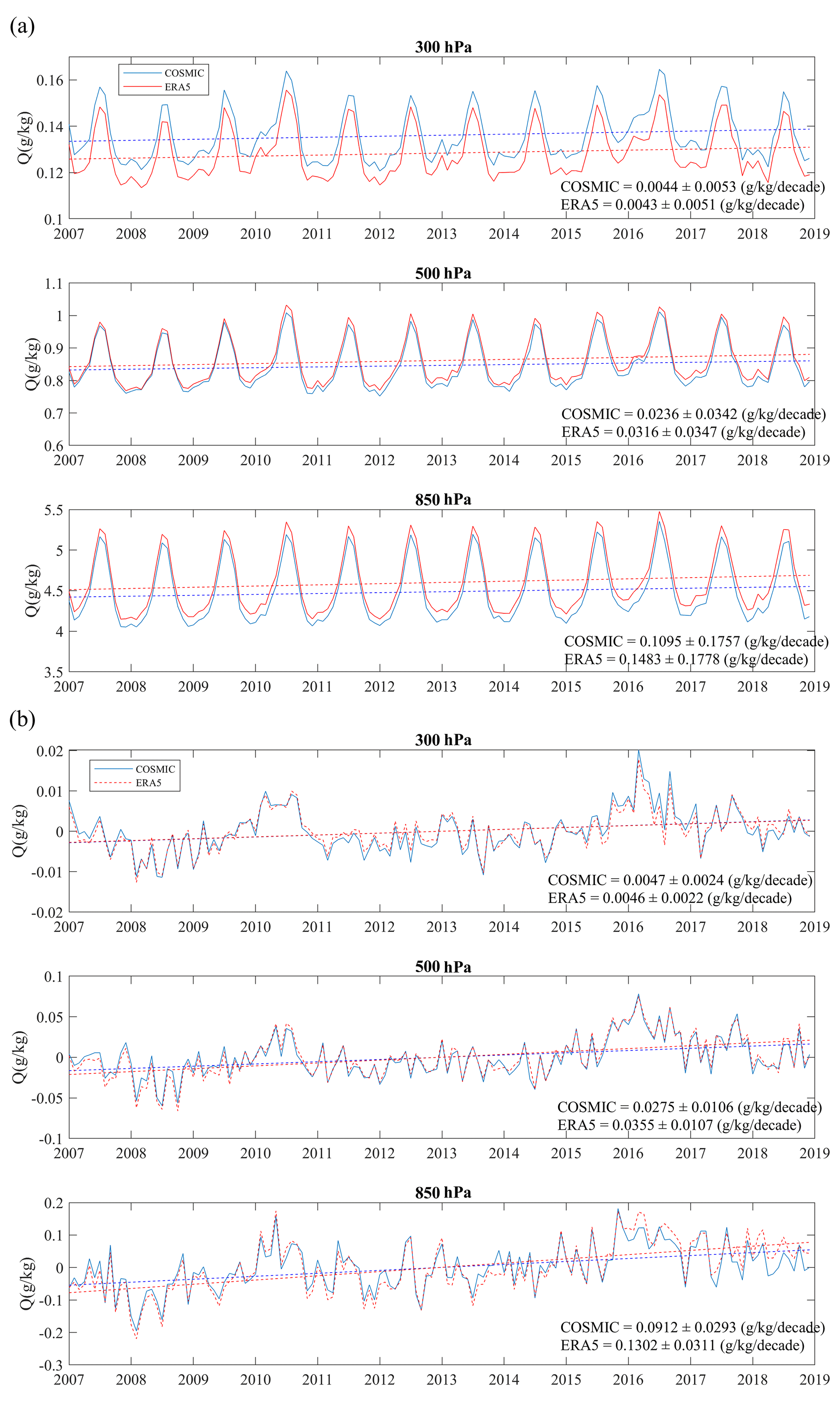
Figure 4(a) Monthly mean time series of COSMIC and ERA5 global mean water vapor data at three pressure levels (solid lines) and linear trend (dashed lines). (b) Time series of sampling-error-removed and deseasonalized monthly mean COSMIC and ERA5 global water vapor data (solid lines) as well as the linear trend (dashed lines). In all panels, red and blue lines are time series (solid lines) and trends (dashed lines) of ERA5 and COSMIC water vapor data, respectively.
It can be seen in Fig. 4a that there were two abnormal water vapor increases around 2010 and 2015–2016 in both the COSMIC and ERA5 time series at all three pressure levels. The abnormal increases in water vapor around 2010 and 2015–2016 were also observed in the long-term total precipitable water monitoring (Mears et al., 2022), which used multiple RO sensors and radiosonde data to construct the time series data. These abnormal water vapor increases were attributed to El Niño, i.e., the warm phase of the El Niño–Southern Oscillation (ENSO). These warm events can enhance surface evaporation, increase tropospheric water vapor, and warm the entire tropical troposphere (e.g., Zveryaev and Allan 2005; Trenberth et al., 2005). The recent 2015–2016 El Niño event broke warming records in the central Pacific according to the Niño3.4 (sea surface temperature – SST – anomalies averaged over the equatorial region at latitude −5 to 5∘ and longitude −150 to 160∘ of the Pacific Ocean) and Niño4 indices (SST anomalies over the region of latitude −5 to 5∘ and longitude −150 to 160∘). The 2015–2016 El Niño event was among the most significant events recorded in this century. During the El Niño event from April 2015 to May 2016, the equatorial Pacific Ocean waters stayed warm for a whole year, reaching peak temperatures in November 2015 (https://www.ecmwf.int/en/newsletter/151/meteorology/2015-2016-el-nino-and-beyond, last access: 7 November 2023). The long period of warm Pacific Ocean temperature significantly impacted the global weather patterns and diminished the seasonal cycles. This also caused anomalies in the seasonal variation of the 2015–2016 global atmospheric water concentration through the coupling between the ocean and atmosphere over the equatorial Pacific Ocean and the atmospheric winds (Fig. 4a).
To quantitatively evaluate the trend of global water vapor, Fig. 4b shows the time series of sampling-error-removed and deseasonalized monthly mean global water vapor of COSMIC and ERA5 at three pressure levels. The slope values, i.e., long-term trends, are derived with linear regression and listed in Table 1 in units of both grams per kilogram (g kg−1) per decade (DQ) and percent (%) per decade (NDQ). In calculating the percent per decade trend, i.e., normalized trend (NDQ), the long-term averaged global mean water vapor (g kg−1) at a given pressure level has been used to normalize the trend with the unit grams per kilogram (g kg−1) per decade.
COSMIC and ERA5 water vapor trend data (Fig. 4) show that the global water vapor trends at three pressure levels are all positive, suggesting an increase in global water vapor concentration during the period from 2007 to 2018, i.e., becoming globally moister, over time at these pressure levels. Many earlier studies reported a rise in global atmospheric water vapor in different periods, e.g., over the period 1979–2001 with ERA-40 reanalysis (Bengtsson, 2004), over the period 1976–2004 using global meteorological data measured by weather stations and marine ships (Dai 2006), and over 1996–2002 with Global Ozone Monitoring Experiment (GOME) data (Wagner et al., 2006). In Chen and Liu (2016), five global PWV datasets, e.g., ECMWF and NCEP reanalysis data, radiosonde, ground GPS stations, and microwave satellite measurements, over the period 2000–2014 were used to derive the trend, and all show a positive global PWV trend. Allan et al. (2022) studied the global-scale changes in water vapor and responses to surface temperature variability since 1979 using coupled and atmosphere-only CMIP6 climate model simulations. In the water vapor trend estimation over the 1988 to 2014 period, Allan et al. (2022) showed a positive increase in global water vapor at the near surface and at 400 hPa as well as column-integrated water vapor from an ensemble of climate model simulations with the CMIP6 historical and Atmospheric Model Intercomparison Project (AMIP) experiments. The period of COSMIC RO data studied in this paper (2007 to 2018) partially overlaps with the simulations of Allan et al. (2022). The increasing trend in the global atmospheric water vapor concentration at the three pressure levels considered in our trend analysis is generally consistent with the results from Allan et al. (2022). It was suggested that an increasing trend in water vapor could be a response to the surface temperature increase (Held and Soden, 2006; Santer et al., 2006; Zhang et al., 2013).
Table 1 shows that the increasing trends of global water vapor vary from ∼ 2 % per decade to ∼ 4 % per decade from the analysis of both COSMIC and ERA5 data at the three pressure levels. It was also shown by Allan et al. (2022) that in the ensemble historical experimental model simulations, the water vapor increases by 1.53 % per decade and 3.52 % per decade at the surface and at 400 hPa, respectively. Our study shows that the increasing global water vapor trends estimated for the COSMIC data over the period 2007–2018 are 2.03 ± 0.65 % per decade, 3.25 ± 1.25 % per decade, and 3.47 ± 1.47 % per decade at 850, 500, and 300 hPa, respectively, which is in general agreement with the results from in Allan et al. (2022), considering that the two works cover two distinct periods with 8 overlapping years. In Allan et al. (2022), there is an increase in water vapor trend from the surface to 400 hPa by ∼ 2 % per decade. Our work shows an increase in water vapor trend by 1.44 % per decade when the pressure level varies from the near surface (at 850 hPa) to 300 hPa, which is generally consistent.
Table 1Comparison of the global water vapor trends (slope ± 95 % confidence interval) derived from COSMIC and ERA5 data.
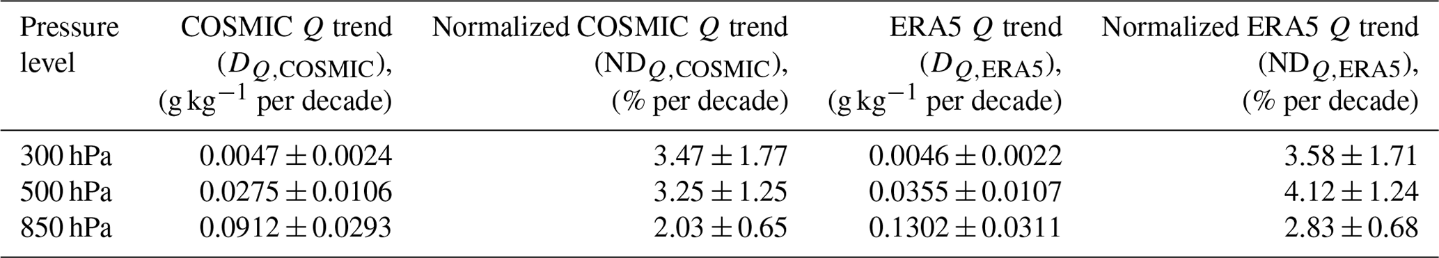
The increasing trend values at 300 hPa derived from COSMIC and ERA5 global water vapor data are consistent. At 500 and 850 hPa, the NDQ,ERA5 values are higher than COSMIC trends by 0.87 % per decade and 0.8 % per decade, respectively, which suggests that ERA5 may overestimate the increase in water vapor during 2007 to 2018. Chen and Liu (2016) showed that the increasing PWV trend from 2000 to 2014 derived from ECMWF data is ∼ 0.37 % per decade larger than the PWV trend derived from the ground GPS station data. The difference between NDQ,ERA5 and NDQ,COSMIC from our analysis at 500 and 850 hPa is about 0.5 % per decade higher than the differences between the trends of ECMWF and ground GPS station PWV data studied by Chen and Liu (2016).
Using the trend results from COSMIC data, we can also see that water vapor trends increase with lower pressure levels. Table 1 shows that the increasing trend at 850 hPa from COSMIC data (NDQ,COSMIC) is lower by 1.44 % per decade and 1.22 % per decade than at 300 and 500 hPa, respectively.
4.2 Comparison of COSMIC and ERA5 latitudinal water vapor trends
To further understand the latitudinal distribution of the water vapor trends, we calculate the slopes of the linear fit for COSMIC (DQ,COSMIC) and ERA5 (DQ,ERA5) at eight 20∘ latitudinal bins distributed from −80 to 80∘. The latitudinal bins above 80∘ in the northern and southern polar regions are excluded from this analysis due to too few COSMIC RO observations. Figure 5 compares slope values of the linear fit of water vapor between COSMIC and ERA5 over eight latitude bins at three pressure levels. The first column of Fig. 5 shows the water vapor trends (DQ) in units of grams per kilogram (g kg−1) per decade. To account for the latitudinal variation of water vapor, the middle column of Fig. 5 shows the water vapor trends (NDQ) normalized by the corresponding long-term latitude-bin-averaged water vapor mean and expressed with the unit of percent per decade. The third column of Fig. 5 shows the latitude-dependent water vapor trend difference (ND, % per decade) between COSMIC and ERA5. Table 2 lists the water vapor trend values of COSMIC and ERA5 for eight latitude bins and at three pressure levels.
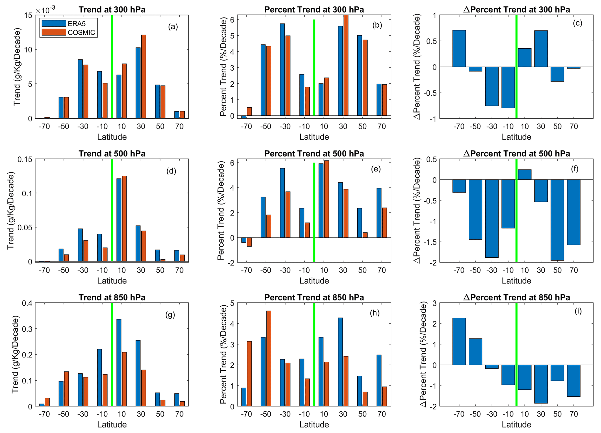
Figure 5(a, d, g) Comparison of the latitude-bin-mean water vapor trends (g kg−1 per decade) between COSMIC and ERA5 data at 300, 500, and 850 hPa, respectively. (b, e, h) Comparison of normalized latitude-bin-mean water vapor trends (% per decade) between COSMIC and ERA5 data at 300, 500, and 850 hPa, respectively. (c, f, i) The difference (COSMIC minus ERA5) of normalized latitude-bin-mean water vapor trend (% per decade) between COSMIC and ERA5 data at 300, 500, and 850 hPa, respectively. The x values on the horizontal axis represent the centers of the 20∘ latitude bins. The green line in each panel separates the Southern (to its left) and Northern (to its right) Hemisphere.
From Fig. 5, the latitude-mean water vapor trends are mostly positive (increasing), and their magnitudes vary substantially with latitude bins at three pressure levels. The only latitude bin with a small negative water vapor trend with large uncertainty is in the −80 to −60∘ southern high-latitude bin at 500 hPa. From the global surface temperature trend analysis by Gu and Adler (2022), there is a mixture of a weak decreasing trend in the surface temperature in the Southern Ocean around the Antarctic and an increasing trend over the Antarctic in the −80 to −60∘ southern latitude bin. However, the uncertainties of estimating the temperature and water vapor trends in this latitude zone are large.
At 300 hPa, the differences in water vapor trends (Fig. 5c) between COSMIC (NDQ,COSMIC) and ERA5 (NDQ,ERA5) consist of positive and negative values with magnitudes less than 0.8 % per decade over the eight latitude bins. In other words, the COSMIC and ERA5 water vapor trends are consistent within 0.8 % per decade over all eight latitude bins. In Fig. 5b, the trends of water vapor change in the four latitude bins over the −60 to −20 and 20 to 60∘ zones are in the range of 4 % per decade to ∼ 6 % per decade, which is higher than the water vapor trends (1.79 % per decade to 2.58 % per decade) of the two equatorial latitude bins (0 to 20 and −20 to 0∘). The southern −80 to −60∘ latitude bin has the lowest water vapor trends (both |NDQ,ERA5| and |NDQ,COSMIC| < 0.6 % per decade) at 300 hPa among the eight latitude bins studied in this paper.
Table 2Latitude-bin-mean water vapor trends (g kg−1 per decade and % per decade) and 95 % confidence interval estimated from COSMIC and ERA5 data at 300, 500, and 850 hPa.
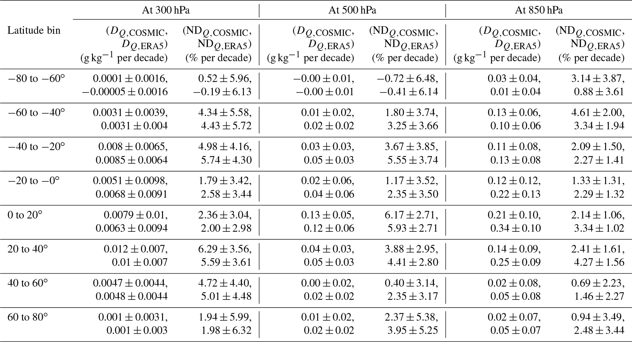
At 500 hPa, both DQ,COSMIC and DQ,ERA5 are the highest (∼ 0.13 g kg−1 per decade) in the 0 to 20∘ latitude bin (Fig. 5d). Regarding the normalized trends of the unit percent per decade, the NDQ,COSMIC and NDQ,ERA5 (% per decade) are all positive except in the −80 to −60∘ latitude bin. Over the latitude bins in the −60 to 80∘ latitude zone, the values of NDQ,ERA5 vary between 2.35 % per decade and 5.93 % per decade, while values of NDQ,COSMIC vary between 0.4 % per decade and 6.17 % per decade. The water vapor trends of NDQ,COSMIC and NDQ,ERA5 in the −80 to −60∘ latitude bin are both quite stable with a weak negative trend of −0.72 % per decade. Figure 5f shows that the differences between NDQ,COSMIC and NDQ,ERA5 are all negative (−2 % per decade to −0.3 % per decade) except for one small positive difference (0.24 % per decade) at the 0 to 20∘ latitude bin. The smaller global water vapor trend from COSMIC at 500 hPa compared to the trend from ERA5, as shown in Table 1, mainly comes from the latitude bins with negative (Fig. 5f). This analysis indicates that at 500 hPa, both ERA5 and COSMIC water vapor data confirm the increasing trends in all the latitude zones from −60 to 80∘, and the trends estimated from COSMIC water vapor data are lower than those from ERA5 in most latitude bins except the 0 to 20∘ equatorial bin.
At 850 hPa, the water vapor trends are all positive from the COSMIC and ERA5 data analysis over eight latitude bins at three pressure levels (Fig. 5g and Table 2). Regarding the absolute water vapor trend, i.e., in units of grams per kilogram (g kg−1) per decade, the water vapor growth peaks in the 0 to 20∘ bin and decreases as the latitude increases toward higher latitudes. The overall magnitudes of water vapor trends are larger than 0.1 g kg−1 per decade from ERA5 and COSMIC data estimated for all latitude bins in the −40 to 40∘ latitude zone. The DQ,ERA5 is larger by 0.1 to 0.13 g kg−1 per decade than DQ,COSMIC in all of the latitude bins from −20 to 40∘. The normalized water vapor trends in Fig. 5h and Table 2 show that both NDQ,COSMIC and NDQ,ERA5 have substantial variabilities (between 0.69 % per decade and 4.61 % per decade) among all of the latitude bins. Figure 5i shows that NDQ,COSMIC is lower than NDQ,ERA5 over all the latitude bins from −40 to 80∘ and NDQ,COSMIC is larger than NDQ,ERA5 over all the latitude bins from −80 to −40∘. The magnitudes of the difference (ND in all the latitude bins from −60 to 80∘ are less than 2 % per decade. This indicates that the relatively lower global water vapor trends estimated from COSMIC data compared to ERA5 data at the 850 hPa level (as presented in Table 1) are mainly due to the lower values of COSMIC trends within the middle- and low-latitude bins.
5.1 Global map of the 10∘ × 10∘ COSMIC and ERA5 water vapor trends
To quantify and compare the global distribution of the regional water vapor trends derived from COSMIC and ERA5 data, we grouped the collocated global water vapor data over 12 years (2007–2018) into 10∘ × 10∘ latitude–longitude grids. We followed the procedure of estimating the water vapor trend outlined in Appendix A2 to calculate the trends (DQ,COSMIC, NDQ,COSMIC, DQ,ERA5, NDQ,ERA5) for the globally distributed 10∘ × 10∘ RoIs. When the grid size is limited to 10∘ × 10∘, there are missing monthly data for specific RoIs due to the limited orbital coverage of COSMIC. Figure 6 shows the percentage of missing monthly data distribution over the 2007 to 2018 period in the global 10∘ × 10∘ grids. The grids with no missing monthly data during this period are shown as white blanks. The grids with substantial missing monthly data are mostly found over northern and southern polar regions with latitudes greater than 70∘. Missing COSMIC RO data are prominent over the regions covering the Tibetan Plateau, specifically at pressure levels of 500 and 850 hPa. The absence of RO data in these regions can be attributed to the lower atmospheric pressure prevailing over areas at an average altitude of around 4 km. Our 10∘ × 10∘ RoI-based trend analysis excludes the grids with more than 1.5 % missing monthly data at 850 hPa. In other words, grids with > 2 months of missing monthly data are excluded from the trend calculation. The effects of sampling error removal on regional water vapor trend analysis uncertainty are discussed in Appendix A3.

Figure 6The percentage of missing monthly data over the 2007 to 2018 interval on the global 10∘ × 10∘ grids. The percentage of missing data is shown as color-coded. Grids with complete monthly data and without gaps, i.e., covering all months, are represented as white blank spaces.
Figure 7 shows the global distribution of COSMIC and ERA5 water vapor trends (DQ,COSMIC and DQ,ERA5) and their difference () at 500 and 850 hPa. The distributions of COSMIC and ERA5 water vapor trends at 300 hPa have smaller regional variations. They are not shown in Fig. 7. In Sect. 4, Figs. 4 and 5 suggest that the global water vapor trends are increasing. The latitude-bin-based water vapor trends are increasing in low and middle latitudes at all three pressure levels we studied. Figure 7a–d shows that both COSMIC and ERA5 data indicate substantial regional variabilities in the global distribution of the water vapor trends. The magnitude of water vapor trends peaks near the Equator and decreases as it approaches the polar regions, where the atmosphere is drier.
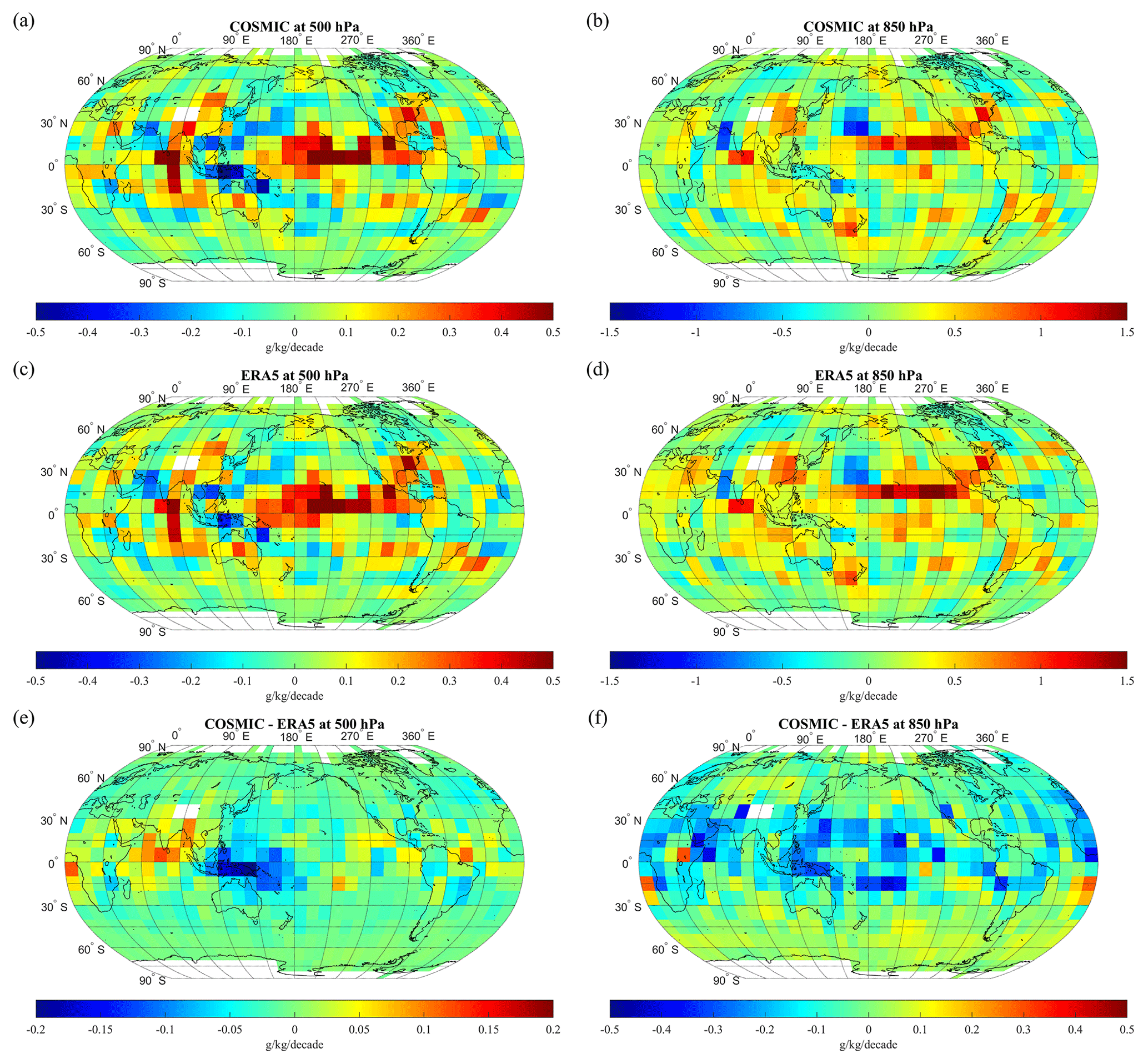
Figure 7(a, b, c, d) The global distribution of water vapor trends (g kg−1 per decade) in 10∘ × 10∘ grids derived from long-term COSMIC (a, b) and ERA5 (c, d) data. (e, f) The global distribution of the water vapor trend difference (g kg−1 per decade) between COSMIC and ERA5 (COSMIC minus ERA5). The left and right columns are derived with water vapor data at 500 and 850 hPa, respectively.
Near the Equator, at 500 and 850 hPa, both DQ,COSMIC and DQ,ERA5 are strongly positive, i.e., becoming moister over time, around 180 to 240∘ longitude and 10 to 20∘ latitude in the equatorial Pacific Ocean. This region in the Pacific Ocean with a strong positive water vapor trend is encased at the west side by two regions with negative water vapor trends located around latitude 20∘ and longitude 130∘ as well as latitude −10∘ and longitude 130∘, which are on the northern and southern side, respectively. These two regions are located between the western Pacific and the eastern Indian Ocean, where sizable regional moisture flux convergence occurs (Fig. 2). A strongly increasing water vapor trend in the equatorial Pacific Ocean and decreasing water vapor trend near the region between the western Pacific and the eastern Indian Ocean are more prominent at 500 hPa than at 850 hPa. At 500 hPa, the negative water vapor trends are extended to northern Australia and southern Asia, covering the Indo-Pacific warm pool region (De Deckker, 2016).
Sea surface temperature has been increasing in the western Pacific during recent decades (e.g., Gu and Adler, 2022). There is a high correspondence with regard to the trends in sea surface temperature and tropospheric water vapor in the western Pacific during recent decades (e.g., Gu and Adler, 2013). It was shown by Chen and Liu (2016) that the moderate increase in surface temperature over the Pacific Ocean could cause the PWV to increase in the equatorial region of the Pacific Ocean and decrease in this Indo-Pacific warm pool region, which is what we observe here. Further quantitative analysis of trends at selected locations in the Pacific Ocean (site no. 6 in Fig. 8) and the Indo-Pacific warm pool region (site no.4 in Fig. 8) will be performed in the following sections.
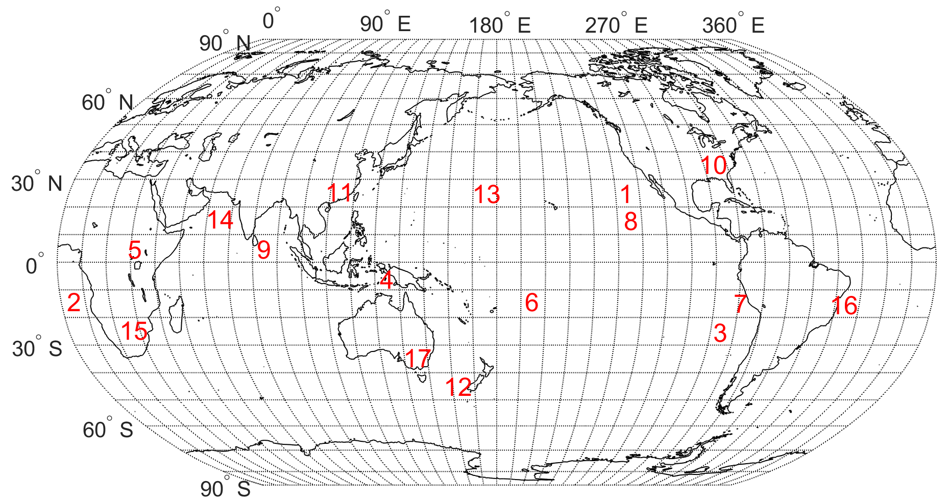
Figure 8Center locations of selected sites for regional analysis of water vapor trends.
In the Indian Ocean, the region in the Laccadive Sea near the northern edge of the Indian Ocean (latitude: 0 to 10∘; longitude: 70 to 90∘) has strong increasing water vapor trends at 850 hPa. At 500 hPa, the region with strong positive water vapor trends expands to a larger region (latitude: −20 to 10∘; longitude: 80 to 90∘). This region is affected by the monsoon climate over the south of the Himalayas. The monsoon climate influences water vapor variability and trends through moisture transport (An et al., 2015; Turner and Annamalai, 2012). The variability in water vapor trends in a region experiencing a monsoon climate is closely tied to the alternating wet and dry phases. Factors such as the strength and duration of the monsoon, the temperature of the ocean waters, and atmospheric circulation patterns all play a role in determining the extent of moisture transport and its impact on water vapor levels. Changes in sea surface temperatures due to global warming can affect the intensity and timing of monsoon patterns, leading to shifts in moisture transport and potentially altering the variability of water vapor content in the affected regions. The Indian Ocean is an essential part of the coupled Indian monsoon system because it feeds the moist convection over both land and ocean. It is shown that the Indian Ocean has been warming up in recent decades (Gu and Adler, 2022). The warming of the Indian Ocean can be the main driver for this region's positive water vapor trend (latitude: 0 to 10∘; longitude: 70 to 90∘). The region near the Gulf of Oman in the Arabian Sea (latitude: 10 to 30∘; longitude: 60 to 70∘) has strong decreasing water vapor trends at 850 hPa. At 500 hPa, this region with negative water vapor trends expands to the area with latitude 10 to 30∘ and longitude 50 to 80∘ and covers the northern coast. The variability of the water vapor trends in this region may arise from the moisture transport influenced by the monsoon climate.
Over land, a significantly increasing water vapor trend at 850 hPa can be observed around the region in the eastern United States (latitude: 30 to 40∘; longitude: 270 to 280∘) and over the region near southeastern China (latitude: 20 to 40∘; longitude: 110 to 130∘).
Figure 7e and f show the spatial distribution of the , i.e., the water vapor trend differences between COSMIC and ERA5, at 500 and 850 hPa, respectively. At 500 hPa, the negative differences () are primarily distributed in the regional box (latitude: −10 to 10∘; longitude: 120 to 170∘) where the Indo-Pacific Ocean region is located, and the decreasing water vapor trends are observed by both COSMIC and ERA5. The difference is positive at 500 hPa, i.e., , in the northern Indian Ocean and near its north coast. At 850 hPa, the difference is primarily negative, with the COSMIC trend being lower than ERA5 in tropical areas. Such dominantly negative differences between DQ,COSMIC and DQ,ERA5 in tropical regions (30∘ S to 30∘ N) at 850 hPa determine the lower global and low-latitude DQ,COSMIC in comparison with DQ,ERA5 as shown in Tables 1–2 and Fig. 5.
In the following sections, we selected a few representative 10∘ × 10∘ grids (sites) to quantitatively characterize the spatial variability of COSMIC and ERA5 water vapor trends. The center locations of these selected 10∘ × 10∘ grids are shown in Fig. 8. These sites include stratocumulus-cloud-rich sites (site nos. 1–3 discussed in Sect. 5.2) and sites with a notable difference between ERA5 and COSMIC trends (site nos. 4–7 discussed in Sect. 5.3), which can help quantitatively understand the regional difference of water vapor trends between COSMIC and ERA5. To quantitatively characterize the large regional variabilities, i.e., mixed with strong increasing and decreasing, of water vapor trends shown in Fig. 7a–d, we also identified and analyzed several sites with notable increasing (moister, site nos. 8–12) and decreasing (drier, site nos. 13–17) water vapor trends. The analysis results for these sites are presented in Appendix A4.
5.2 Water vapor trends over stratocumulus-cloud-rich regions
The first set of sites (site nos. 1–3 in Fig. 8) we selected is over stratocumulus-cloud-rich regions. These three sites are selected according to the stratocumulus-cloud-rich regions identified by Wood et al. (2011), Wood (2012), and Ho et al. (2015). Stratocumulus clouds are typically shallow and occur at low altitudes (below 2 km) due to weak convective currents with drier and stable air above, preventing continued vertical development. Stratocumulus clouds usually occur over subtropical and polar oceans. Over regions with frequent stratocumulus clouds, it is challenging to accurately estimate water vapor at low altitudes in the ECMWF assimilation (Lonitz and Geer, 2017).
On the other hand, the RO signal can penetrate the cloud layer because the wavelengths for L1 and L2 frequency of RO signals are around 19 and 24.2 cm, respectively, which are much larger than the size of cloud water droplets and ice crystals (Kursinski et al., 1997). The water vapor retrieval from RO data is not affected by the cloud. This study helps to determine whether there are differences between COSMIC and ERA5 water vapor trends over these stratocumulus-cloud-rich regions and quantify the difference. Therefore, we compare the near-surface water vapor trend of ERA5 and COSMIC at 850 hPa over three stratocumulus-cloud-rich regions. Table 3 lists the water vapor trends at 500 and 850 hPa over three sites in the ocean: west of the Baja coast (no. 1), west of Africa (no. 2), and west of South America (no. 3), derived from COSMIC and ERA5 data.
Table 3Water vapor trends over three selected stratocumulus-cloud-rich sites.
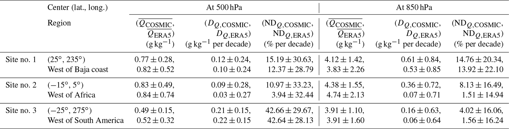
At 850 hPa, COSMIC and ERA5 data show that these three sites have comparable mean water vapor (around 4 g kg−1). At 500 hPa, site no. 3 has a lower mean water vapor than the other two sites. These three sites have positive water vapor slopes at 500 and 850 hPa. At 850 hPa, site no. 1 has the strongest increasing trend of water vapor and NDQ,COSMIC (14.76 % per decade) is comparable to NDQ,ERA5 (13.92 % per decade). For site no. 2 and no. 3, there are significant differences between the trends estimated with COSMIC and ERA5 data at 850 hPa. For example, the increasing trend estimated from COSMIC (NDQ,COSMIC) is about 6.62 % per decade higher than NDQ,ERA5 for site no. 2 (Table 3). For site no. 3, the NDQ,COSMIC is higher than NDQ,ERA5 by 2.46 % per decade. This analysis indicates that for two of the three selected sites around the stratocumulus-cloud-rich regions, the estimated water vapor trends from COSMIC at 850 hPa can be significantly higher than those estimated from ERA5 data. The possible cause of smaller trends from ERA5 water vapor data over stratocumulus-cloud-rich regions could be the difficulty in accurately estimating water vapor at low altitudes from ERA5 reanalysis data compared with COSMIC RO measurements that are unaffected by stratocumulus clouds (Lonitz and Geer, 2017).
5.3 Sites with a notable water vapor trend difference between ERA5 and COSMIC
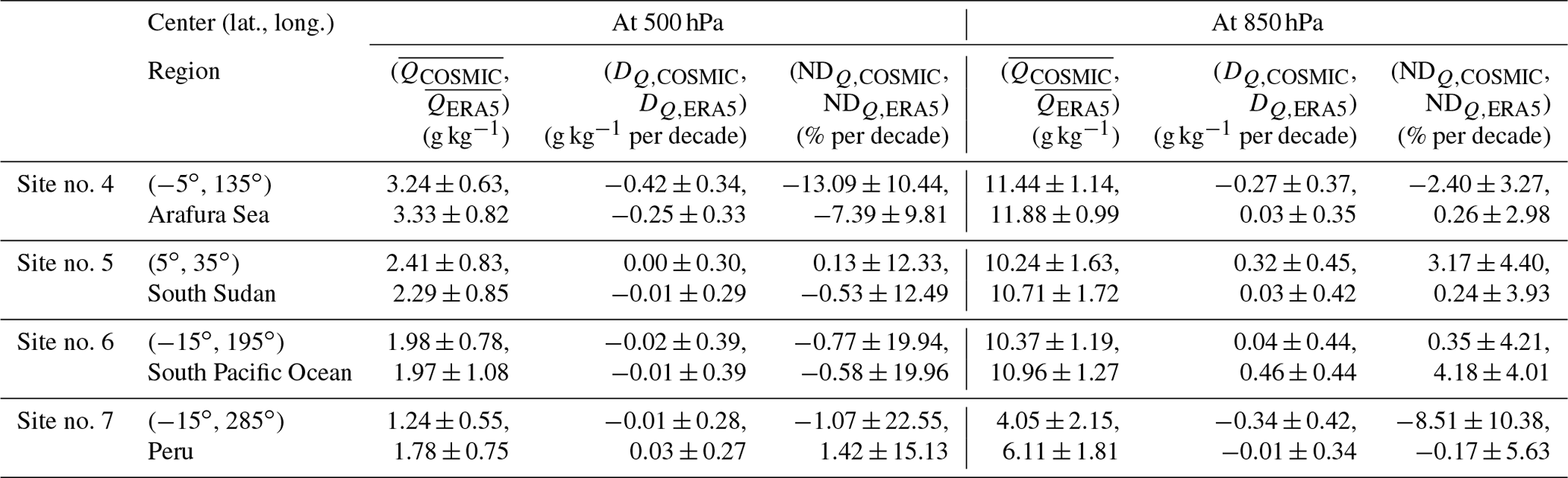
Comparing regional water vapor trends between COSMIC and ERA5 data and quantifying their differences contribute to validating both datasets. In particular, it can identify regions where the reanalysis model could exhibit constraints. In this section, we select a few sites with a notable trend difference between COSMIC and ERA5 to quantitatively understand the magnitude of the differences and the distribution of these sites. To identify these sites, we first searched the 10∘ × 10∘ global map of the water vapor trend difference between COSMIC and ERA5 (Fig. 7e and f shown in Sect. 5.1). We identified the regions with the largest positive or negative water vapor trend difference between COSMIC and ERA5. Within these regions, we selected one representative 10∘ × 10∘ grid in each region as the site of interest. The estimated water vapor trends for COSMIC and ERA5 over these sites with notable trend differences are listed and compared in Table 4. Sites no. 4 and no. 6 are over the ocean, and sites no. 5 and no. 7 are over land. Sites no. 4, no. 5, and no. 6 are moisture-rich. Site no. 4 is located in the Indo-Pacific Ocean region, which suggests large uncertainty in the characterization of DQ,ERA5 in this region. Site no. 5 is among the few sites (see Fig. 7f in Sect. 5.1) with DQ,COSMIC larger than DQ,ERA5 (by 0.29 g kg−1 per decade) at 850 hPa. Site no. 6 is a typical low-latitude site with DQ,COSMIC less than DQ,ERA5. For site no. 7 in Peru, COSMIC shows a much steeper decreasing trend, lower by −8.34 % per decade, than ERA5 at 850 hPa. This 10∘ × 10∘ grid of site no. 7 is mixed with the Andes Mountains on the eastern portion of the grid and the Pacific Ocean on the west. There are no 850 hPa RO data over the Andes Mountains (over 6 km in altitude). The RO water vapor trend data mainly come from the Pacific Ocean in the 10∘ × 10∘ grid of site no. 7. The COSMIC water vapor trend indicates that site no. 7 has decreased near-surface water vapor from the period 2007 to 2018, while ERA5 data suggest no significant long-term change in the amount of water vapor. From the linear trend study of global surface temperature during 1998–2020 by Gu and Adler (2022), there is a trend of decreasing ocean surface temperature (∼ −0.1 K per decade) near site no. 7, which matches the decrease in water vapor observed by COSMIC. Site no. 7 is situated in close proximity to site no. 3 and falls within an area where there is a frequent presence of low-height stratocumulus clouds (Wood, 2012), which makes it more challenging to accurately estimate water trends from ERA5 data than from COSMIC data.
The dominantly negative trend differences between DQ,COSMIC and DQ,ERA5 for low-latitude regions at 850 hPa (see Fig. 7f in Sect. 5.1) and the notable large trend difference between COSMIC and ERA5 over site nos. 4–7 are concentrated within the northern and southern boundaries of the Intertropical Convergence Zone (ITCZ). The ITCZ encircles Earth near the thermal Equator, where trade winds converge between the northeast (in the Northern Hemisphere) and the southeast (in the Southern Hemisphere). The specific position of ITCZ varies seasonally. The ITCZ has concentrated deep clouds spanning nearly the entire circumference of the equatorial regions, one of the most prominent atmospheric circulation features. Johnston et al. (2021) investigated the distribution and variability of COSMIC-2 water vapor by comparing it to collocated ERA5 and MERRA-2 reanalysis profiles in the tropical and subtropical regions. It was found by Johnston et al. (2021) that the largest moisture differences and weakest correlations were typically observed in regions that experience frequent convection, such as along the ITCZ, over the Indo-Pacific warm pool, and in central Africa. These locations match what we found in our study. Our explanation for such a difference is that for regions with frequent atmospheric circulation, such as deep clouds, the RO retrievals may characterize water vapor distribution and occurrence better than ERA5 due to the cloud-penetrating ability of GPS signal and higher height resolution in RO data to resolve the sharp moisture gradient better.
Table 4Water vapor trends over selected sites with notable COSMIC and ERA5 trend differences.
This paper evaluates the spatiotemporal consistency and difference between UCAR COSMIC (WETPrf) and ECMWF's ERA5 global reanalysis of water vapor data from 2007 to 2018. The analysis of temporal variability focuses on the long-term trends and seasonal variability of COSMIC and ERA5 water vapor data. Spatial variabilities of the global, latitudinal, and regional distribution of COSMIC and ERA5 mean water vapor and trends at three pressure levels (300, 500, and 850 hPa) are analyzed and quantitatively compared. These two water vapor datasets generally show good agreement in spatiotemporal distributions and trends.
The key comparison results of time-averaged water vapor between COSMIC and ERA5 can be summarized as follows.
- i.
There have been coordinated efforts from the Stratosphere–troposphere Processes And their Role in Climate (SPARC) Reanalysis Intercomparison Project (S-RIP) to compare reanalysis datasets such as ERA5 and ERA-Interim using a variety of key diagnostics. The SPARC S-RIP confirmed the significant improvements of the latest version of reanalyses in ERA5 compared to ERA-Interim (Fujiwara et al., 2017). Our study shows that COSMIC water vapor retrievals are more consistent with ERA5 reanalysis data than ERA-Interim. This suggests that although the UCAR COSMIC 1D-Var retrieval used ERA-Interim as the background model (see Sect. 2.2), the impacts from ERA-Interim on the UCAR 1D-Var retrieval processing are minimal.
- ii.
At 300, 500, and 850 hPa, the differences between COSMIC water vapor retrievals and water vapor from ERA5 over the globe are 5.67 ± 34.30 %, −1.86 ± 30.09 %, and −2.30 ± 21.21 %, respectively. Ho et al. (2010) and Shao et al. (2021b) showed systematic negative water vapor biases below 5 km for RO retrievals compared to radiosonde data. Such negative water vapor biases can be traced to the negative RO bending angle biases compared to the reanalysis model (Ho et al., 2020a). The negative water vapor biases below 5 km, e.g., at 500 and 850 hPa, as studied here, are mainly due to the underestimation of water vapor in RO retrieval in the presence of atmospheric super-refraction or ducting in the moisture-rich low troposphere (Sokolovskiy, 2003; Ao et al., 2003; Xie et al., 2006; Ao, 2007). Super-refraction occurs when the vertical atmospheric refractivity gradient exceeds a critical refraction threshold, i.e., in the presence of a sharp change in refractivity. Such a sharp change often exists around the planetary boundary layer, where sharp vertical gradients in moisture and temperature inversion are frequently observed. To address the negative moisture biases in RO retrieval and account for super-refraction or ducting, there are efforts to improve the 1D-Var retrieval algorithm by incorporating the reconstruction method introduced by Xie et al. (2010). Our study shows that the negative water vapor biases at 850 hPa are dominantly in the −40 to 40∘ (tropical and subtropical) moisture-rich regions. This study shows that the global (Fig. 4 and Table 1) water vapor trends are generally consistent with ERA5 at 500 and 850 hPa, although negative water vapor biases are present at these two pressure levels.
- iii.
A latitude dependence study shows the asymmetry in the latitudinal distribution of water vapor between the Northern and Southern Hemisphere. There was a more rapid decrease in water vapor from the low-latitude tropical to the polar region in the Southern Hemisphere than in the Northern Hemisphere. The interhemispheric water vapor difference can be traced to the interhemispheric difference in temperature (Feulner et al., 2013).
The key findings from the trend estimates for the period from 2007 to 2018 COSMIC and ERA5 water vapor data at global, latitudinal, and regional (10 by the 10∘ grid) levels are summarized as follows.
- i.
The anomalous water vapor increase around 2015–2016 is identifiable in the COSMIC and ERA5 time series of water vapor data at all three pressure levels and was attributed to an El Niño event from April 2015 to May 2016.
- ii.
COSMIC and ERA5 global water vapor shows increasing trends at three pressure levels. The positive global water vapor trends from COSMIC data are 3.47 ± 1.77 % per decade, 3.25 ± 1.25 % per decade, and 2.03 ± 0.65 % per decade at 300, 500, and 850 hPa, respectively. The positive global water vapor trends can be a response to the global surface temperature increase (Held and Soden, 2006; Santer et al., 2006; Zhang et al., 2013; Chen and Liu, 2016; Ho et al., 2018; Allan et al., 2022).
- iii.
The latitude-mean water vapor trends are mostly positive (increasing) except in the southern −80 to −60∘ latitude zone and show substantial variability (between 0.4 % per decade and ∼ 6 % per decade) with latitude bins. The trend difference between COSMIC and ERA5 is less than 2 % per decade for most latitude bins at three pressure levels.
- iv.
The regional distribution of water vapor trends in the tropical and subtropical regions has large local variabilities and is mixed with substantial increasing and decreasing trends. The regions in the equatorial Pacific Ocean with strong increasing water vapor trends are identified. Negative (decreasing) water vapor trends, i.e., becoming drier, are observed near the Indo-Pacific Ocean region at 500 and 850 hPa.
- v.
The assessment of regional water vapor trend variability and consistency between COSMIC and ERA5 indicates the following.
- a.
A significant difference in the water vapor trends was estimated between COSMIC and ERA5 data at 850 hPa over two stratocumulus-cloud-rich ocean sites. The possible cause of smaller trends from ERA5 water vapor data over stratocumulus-cloud-rich regions could be the difficulty in accurately estimating water vapor at low altitudes in ERA5 reanalysis data (Lonitz and Geer, 2017) compared with COSMIC RO measurements that are unaffected by stratocumulus cloud.
- b.
Over land, significantly increasing water vapor trends at 850 hPa can be observed around the region in the southern United States (latitude: 35∘, longitude: 275∘) and the region near southeastern China (latitude: 25∘, longitude: 115∘). Two sites in southern Africa and Australia have long-term negative water vapor trends at 850 hPa, which can cause a regional long-term drier atmosphere and intensified droughts. The site in Australia has huge negative trends (less than −10 % per decade at 850 hPa) (becoming drier) from both COSMIC and ERA5 water vapor trends, which is consistent with Dai (2006) and Zhang et al. (2018).
- c.
The differences between the water vapor trends of COSMIC and ERA5 are primarily negative in the tropical regions at 850 hPa. At 500 hPa, the negative differences are mainly distributed in the Indo-Pacific Ocean region. In contrast, the positive difference is located near the northern coast of the Indian Ocean.
- a.
From our analysis, the regions with notable trend differences between COSMIC and ERA5 are mostly distributed within the northern and southern boundary of the ITCZ area, over the Indo-Pacific warm pool or central Africa. These regions experience frequent convection, such as deep convective clouds. Because of the cloud penetration property of GNSS signals and higher height resolution of RO retrievals, the height and temporal distribution of water vapor can be better characterized in RO retrievals than ERA5 in the presence of convection, such as deep clouds. The better representation of water vapor in RO data may cause the difference in water vapor trend estimation between COSMIC and ERA5 over these regions, which will need further studies with other long-term water vapor data. In particular, comparing long-term ground-based GNSS and GPS data (Mears et al., 2017) as well as radiosonde data (Patel and Kuttippurath, 2022) can help address the biases and trend differences between RO and the reanalysis model over land.
In analyzing long-term water vapor trends from RO data, it is important to remove sampling errors to correct the biases due to RO data's limited time and location coverage. The sampling error removal accounts for the difference between the orbital-specific distribution of COSMIC RO measurements and uniformly distributed global ERA5 data. After applying sampling error removal, our estimations indicate a reduction in uncertainty by approximately 4.8 times at 500 hPa and 3.1 times at 850 hPa. This magnitude of uncertainty reduction is close to that shown by Gleisner et al. (2020). Our study also shows that the COSMIC water vapor retrievals are more consistent with ERA5 than ERA-Interim model data and confirms that ERA5 has significantly more improved quality than ERA-Interim. This paper's overall global water vapor trends are close to the trend results from Allan et al. (2022). We postulate that using other global reanalysis models, such as NCEP and MERRA-2, may have compatible global trends but differ in regional trends from our results, which will need further evaluation.
This paper compares 12 years of COSMIC data from 2007–2018 with ERA5 reanalysis data. As the follow-on mission of COSMIC, the COSMIC-2 constellation with six satellites has produced RO data since 2019 (Ho et al., 2020b; Ho et al., 2022). In addition, commercial RO sensors such as Spire and GeoOptics (Chen et al., 2021) as well as the upcoming RO sensors on board MetOp Second Generation and other RO missions continue to augment RO data's temporal and spatial coverage. These growing RO datasets combined with the historical multiple RO mission data will provide the opportunity to establish consistent long-term CDR-grade global temperature, water vapor, and derived climatology data products. It is important to emphasize that consistently processed temperature and water vapor data with the same excess phase to bending angle and 1D-Var retrieval models is critical to establish such long-term CDR-grade datasets from multiple RO mission data.
A1 Seasonal variability of COSMIC and ERA5 water vapor distribution
To understand the seasonal variability of water vapor at different pressure levels, we show the annual variation of mean water vapor over 12 months in eight latitudinal bins (20∘ bins from −80 to 80∘ in latitude) in Fig. A1a, c, and e and A2a, c, and e at 300, 500, and 850 hPa pressure levels for the Southern and Northern Hemisphere, respectively. Each month's 12-year (2007 to 2018) water vapor data in each latitude bin have been averaged for COSMIC and ERA5. Figures A1a, c, and e and A2a, c, and e show that the water vapor is high (wet) in the summer and low (dry) in the winter for the corresponding hemisphere at all three pressure levels. The latitudinal variability and seasonal variability of water vapor differences between COSMIC and ERA5 are further quantified as the relative difference (ΔQCOSMIC−ERA5(%)) in Figs. A1b, d, and f and A2b, d, and f for the Southern and Northern Hemisphere, respectively. Figures A1a, c, and e and A2a, c, and e show the overall agreement in seasonal variability between COSMIC and ERA5 at three pressure levels over the Northern and Southern Hemisphere. We can use COSMIC data as a reference to evaluate the overall seasonal variability in different latitude zones. We extracted the summer maximum (Qmax,COSMIC) and winter minimum (Qmin,COSMIC) monthly mean COSMIC water vapor from Figs. A1 and A2.
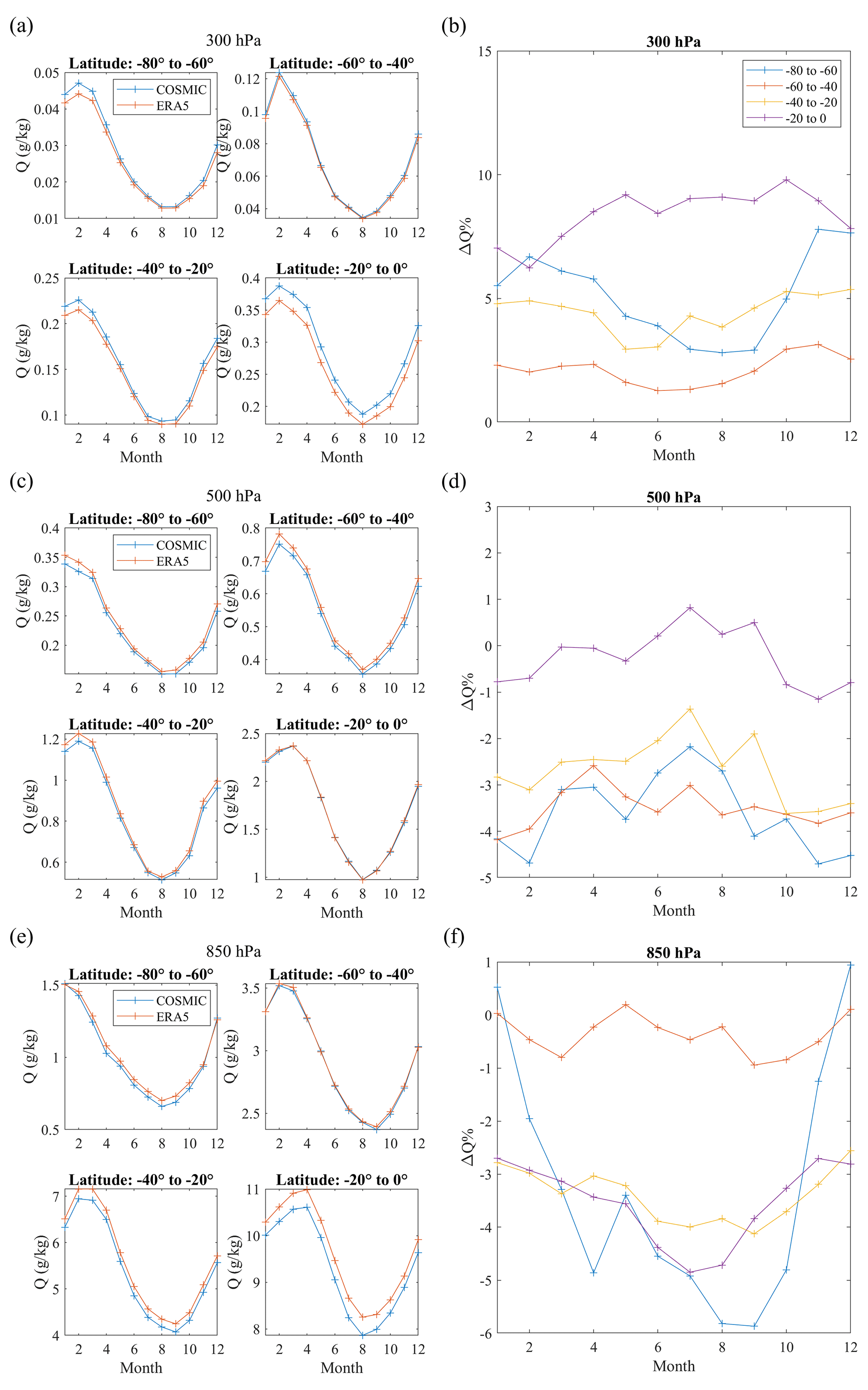
Figure A1(a, c, e) Comparison of seasonal variability (over 12 months) between COSMIC and ERA5 water vapor data in four Southern Hemisphere latitude bins at 300, 500, and 850 hPa, respectively. (b, d, f) Seasonal variation of the percent difference between COSMIC and ERA5 water vapor data grouped in four Southern Hemisphere latitude bins at 300, 500, and 850 hPa, respectively.
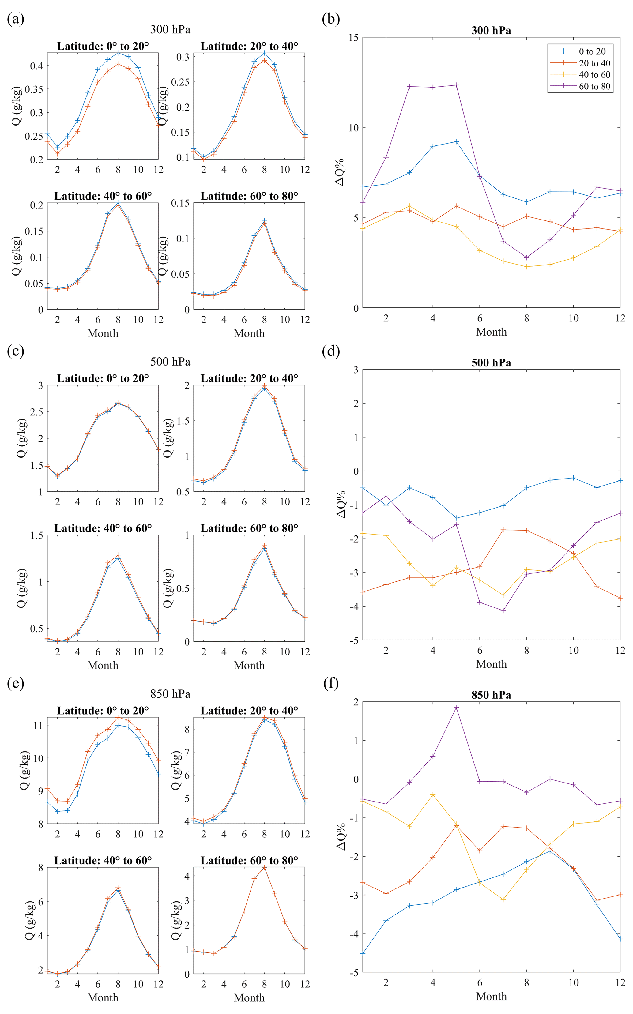
In Fig. A3, we show the summer maximum and winter minimum monthly mean COSMIC water vapor and the annual water vapor variation magnitude defined as at three pressure levels. Over all three pressure levels, the two low-latitude bins (−20 to 0 and 0 to 20∘) both have comparable Qmax,COSMIC, Qmin,COSMIC, and , which suggests that the mixture of water vapor in these two southern and northern latitude zones is quite efficient at all three pressure levels. As approaching higher latitudes in bins with |latitude| > 20∘, the Southern Hemisphere atmosphere is generally drier than the matching latitude zones in the Northern Hemisphere at all three pressure levels. Figure A3 also shows that the seasonal water vapor variabilities, i.e., , are more significant in the Northern Hemisphere than in the Southern Hemisphere for latitude zones above 20∘ at all three pressure levels.
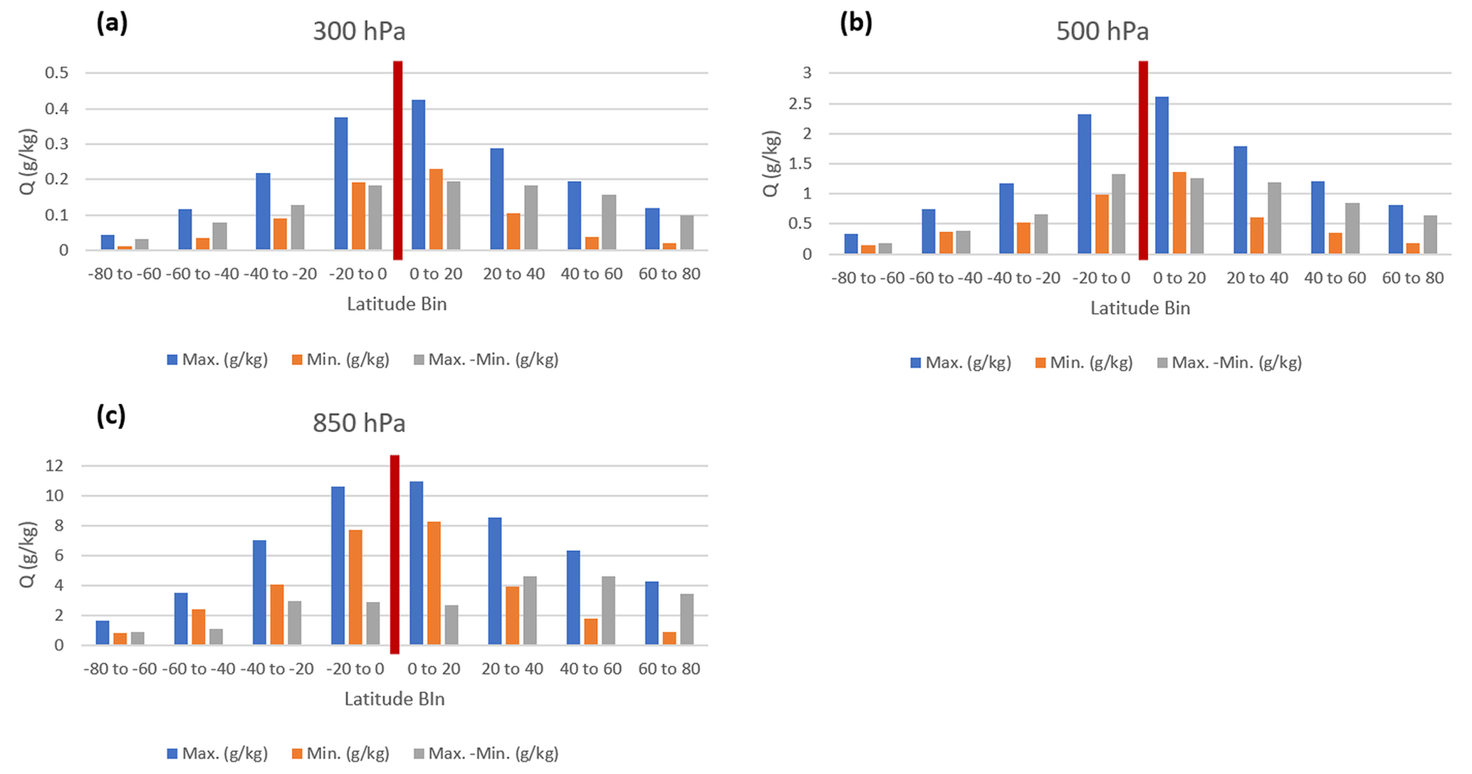
Figure A3Maximum, minimum, and maximum–minimum annual monthly water vapor statistics at three pressure levels of (a) 300, (b) 500, and (c) 850 hPa from COSMIC retrievals. The vertical red line in each panel separates the latitude bins in the Southern (to its left) and Northern (to its right) Hemisphere.
Next, we quantify the difference in the seasonal variability between the COSMIC and ERA5 water vapor data. As shown in Figs. A1b and A2b, at 300 hPa, ΔQCOSMIC−ERA5 (%) values are all positive, i.e., QCOSMIC > QERA5, with values ranging from 1 % to 12.5 % over 12 months and in both hemispheres. The most substantial seasonal variability in the peak-to-valley value of annual ΔQCOSMIC−ERA5 (%) occurs in the northern 60 to 80∘ latitude bin with seasonal variation around ∼ 8 % from March to August. The high-latitude (60 to 80∘) and low-latitude (0 to 20∘) bins in both Northern and Southern Hemisphere all have a peak-to-valley value of annual ΔQCOSMIC−ERA5 (%) higher than 4 %. For middle-latitude (20 to 60∘) bins in the Northern and Southern Hemisphere, the magnitude of seasonal variation of ΔQCOSMIC−ERA5 (%) is less than 2 %. The latitudinal variability of ΔQCOSMIC−ERA5 (%) agrees with the mean latitudinal values shown in Fig. 3c.
At 500 hPa, Figs. A1d and A2d show that ΔQCOSMIC−ERA5 (%) values are negative over 12 months for all latitude bins except the −20 to 0∘ latitude bin, which has ΔQCOSMIC−ERA5 (%) varying from −1 % to 1 %. The overall peak-to-valley seasonal variabilities of ΔQCOSMIC−ERA5 (%) are in the range of 1 % to 3 %, with the most significant seasonal variability (∼ 3 %) in the 60 to 80∘ high-latitude bin. Such magnitudes of seasonal variability of ΔQCOSMIC−ERA5 (%) at 500 hPa are much smaller than those at 300 hPa, which suggests that using ΔQCOSMIC−ERA5 (%) as the metrics, the water vapor of COSMIC retrieval is more consistent with ERA5 at 500 hPa than at 300 hPa. The latitudinal variability of ΔQCOSMIC−ERA5 (%) at 500 hPa is consistent with the mean latitudinal values shown in Fig. 3f.
At 850 hPa, Figs. A1f and A2f show that ΔQCOSMIC−ERA5 (%) values are dominantly negative over 12 months for all latitude bins except one bin in latitude 60 to 80∘, which has ΔQCOSMIC−ERA5 (%) varying from −0.7 % to 1.2 %. The seasonal variabilities (peak-to-valley variation of annual are weak (< 2.5 %) for all of the latitude bins except the southern high-latitude bin at −80 to −60∘, which has the most significant seasonal variability ∼ 6 %. The latitudinal variability of ΔQCOSMIC−ERA5 (%) at 850 hPa agrees with Fig. 3i.
A2 Method of removing the COSMIC sampling errors for water vapor time series analysis
The steps of calculating the COSMIC sampling error and reconstructing the water vapor time series for trend analysis are detailed below.
-
For an RoI such as the global area, latitudinal bins, or a 10∘ × 10∘ latitude–longitude grid, the collocated water vapor data from COSMIC and ERA5 in that region are accumulated for each month. For COSMIC WETPrf data, the location of the RO profile is used to determine whether the RO data are in the RoI. For a given pressure layer, interpolation over the RO profile pressure levels was carried out for COSMIC water vapor data to derive the water vapor at the specific pressure. The ERA5 data are distributed globally on 0.2∘ latitude–longitude grids, 37 pressure layers, and 6 h intervals. Therefore, we interpolate ERA5 data over latitude–longitude and time at the given pressure level that matches the COSMIC RO observation. With the accumulated monthly COSMIC or ERA5 water vapor data for a given RoI, the monthly mean values at a given pressure level are calculated to form the long-term time series of monthly mean water vapor () for the RoI. Figure A4a shows an example of the long-term time series of COSMIC () and ERA5 () water vapor variation at the 850 hPa pressure level for the 0–20∘ latitude bin RoI in the Northern Hemisphere.
-
Figure A4e shows the monthly sample number of COSMIC RO data that fall into the 0–20∘ latitude bin RoI, with substantial variations over the lifetime of COSMIC when the number of available RO sensors in the COSMIC constellation varies over time. Particularly, there was a continuous decrease in the sample number after the middle of 2013. There are six small satellites (C1E1 to C1E6) in the COSMIC-1 constellation. The service interval and performance of these six satellites vary over time. C1E3 is the first satellite that stopped producing data in mid-2010. C1E2, C1E3, and C1E4 ended their operations over the time interval from 2015 to 2017. C1E1 and C1E6 continued operation until the middle of 2019 and early 2020, respectively. Due to the varying performances and availabilities of C1E1 to C1E6, the time series of the combined valid profile numbers from these six satellites thus reflect the pattern shown in Fig. A4e.
To account for the impacts of the limited and varying sample number on the trend analysis, we need to apply sampling error removal to COSMIC data. The sampling errors are the difference between the sample mean and cell mean, which can be estimated using monthly ERA5 data from 2007 to 2018. Eq. (A1) illustrates the calculation of the sampling error (QSE):
where is the monthly mean of the interpolated water vapor profiles from ERA5 that match the COSMIC RO observations in the RoI at a given pressure level, and is the monthly spatial and temporal mean of the ERA5 water vapor in the RoI at the same pressure level. The sampling error removal is carried out by subtracting monthly QSE from the COSMIC monthly water vapor data using Eq. (A2):
where QCOSMIC_SER represents the COSMIC water vapor data after sampling error removal. For ERA5 data, the application of sampling error QSE removal to essentially recovers . The time series of QCOSMIC_SER are unaffected by the limited and varying sample number of COSMIC RO observations. They are used to construct monthly mean climatology (MMC) water vapor data records and characterize the long-term trend of water vapor variation for a given RoI. Figure A4b compares the time series of QCOSMIC_SER and for the 0–20∘ latitude bin RoI at 850 hPa.
Figure A4d shows the time series of COSMIC sampling error QSE in the 0–20∘ latitude bin. Similar to the COSMIC sampling error data shown in Gleisner et al. (2020) and Shen et al. (2021), there are seasonal oscillations (around 0 g kg−1) in the time series of water vapor sampling error shown in Fig. A4d, which is mainly due to the difference between the orbital-specific distribution of COSMIC RO observations (Ho et al., 2020a) and uniformly distributed global ERA5 data. The nonuniform local time and latitude distribution of COSMIC-1 profiles coupled with the annual variation of the Sun's declination contribute to the seasonal oscillation in the sampling error time series. As the monthly sample number of COSMIC RO data decreases after 2010 (Fig. A4e), QSE appears to have increased amplitudes. Over the interval after the middle of 2017, when the sample number of COSMIC decreases more significantly, QSE appears to have more rapid oscillations.
-
As shown in Fig. A4b, there are substantial seasonal oscillations in the monthly mean water vapor data time series after the sampling error removal. To calculate the long-term trend from the time series data, the monthly mean water vapor data must be deseasonalized to filter out the annual oscillation. This step is carried out by grouping the monthly mean water vapor data of the same month over the 2007–2018 period and calculating the mean as a climate monthly mean. In this way, we have 12-month climate water vapor means that can characterize the annual water vapor variation. The long-term water vapor time series is then deseasonalized by subtracting the corresponding climate monthly mean at each data point. Figure A4c shows an example of the time series of the deseasonalized water vapor for COSMIC and ERA5 at the 850 hPa pressure level in the 0–20∘ latitude bin RoI.
-
Linear regression has been carried out with the deseasonalized time series of water vapor to calculate the slope, i.e., the trend DQ (g kg−1 per decade), of the water vapor variation. The example in Fig. A4c shows the linear fitting curves as dashed red and blue lines for ERA5 and COSMIC data, respectively. The values and 95 % confidence interval of the ERA5 and COSMIC water vapor trends are also listed in the figure.
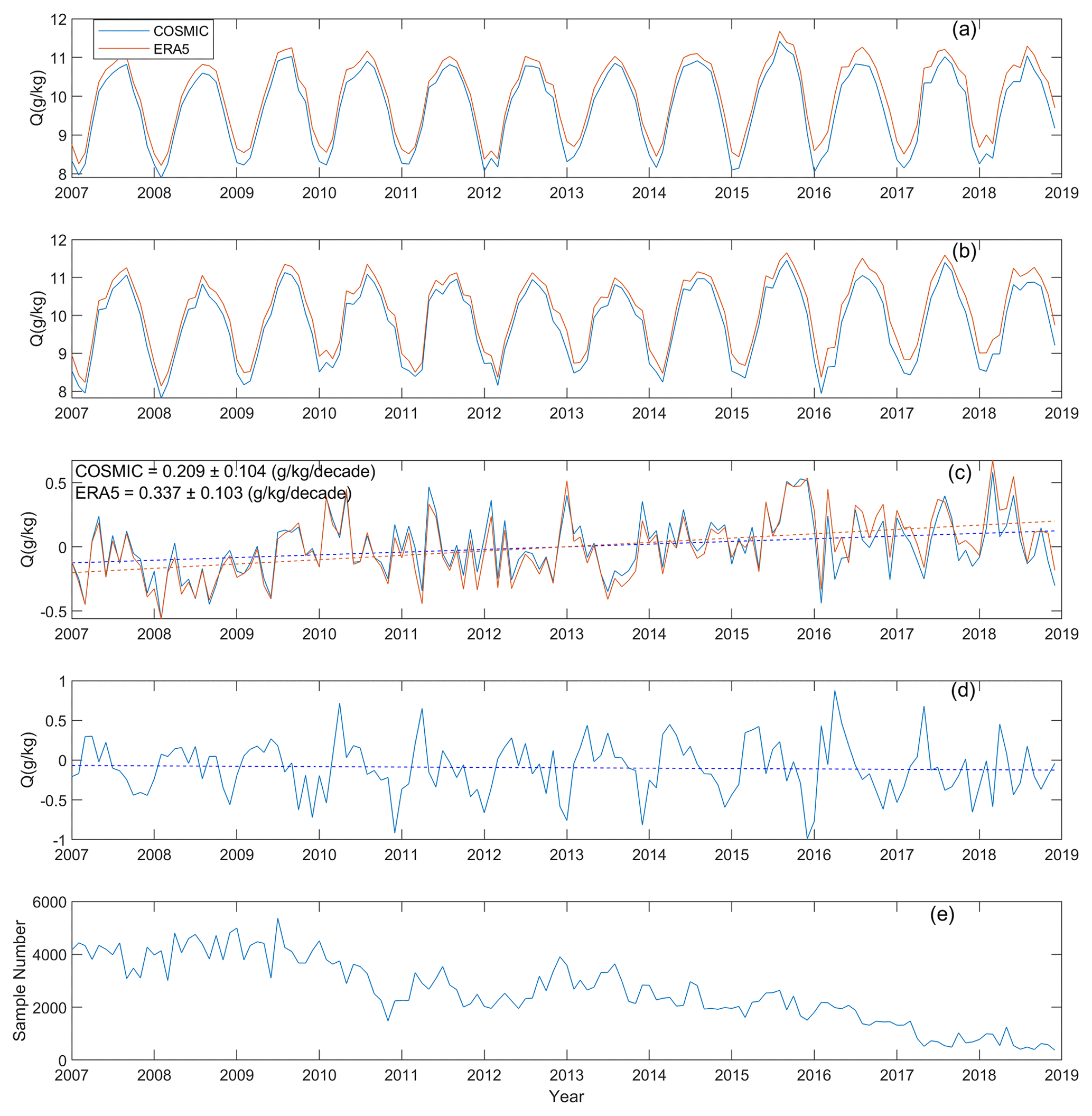
Figure A4Steps to derive the long-term water vapor trend for a given RoI at the pressure level of 850 hPa. (a) The time series of the monthly mean of collocated COSMIC and ERA5 water vapor data in the 0–20∘ latitude bin over the Northern Hemisphere. (b) Time series of COSMIC and ERA5 water vapor data after sampling error removal. (c) The deseasonalized monthly mean COSMIC and ERA5 water vapor data time series over the 0–20∘ latitude bin. Dashed lines are the trends derived from linear regression. In (a)–(c), red and blue lines are time series of ERA5 and COSMIC water vapor data or trends, respectively. (d) Time series of COSMIC water vapor sampling error QSE calculated with Eq. (A1). (e) The sample numbers of COSMIC observations time series fall into the 0–20∘ latitude bin.
A3 Effects of sampling error removal on the uncertainty of the regional water vapor trend analysis
Figure A5a and b show the global (10∘ × 10∘) distribution of trends derived from the sampling error QSE time series at 500 and 850 hPa, respectively. The grids with > 1.5 % missing monthly data over the 2007 to 2018 interval are marked as white blanks in Fig. A5a and b. It can be seen that the sampling error removal does introduce corrections to the regional trends of COSMIC water vapor data. To further evaluate the impacts of the sampling error removal on the uncertainty of the water vapor trend analysis using long-term COSMIC water vapor data, we calculated the histogram distribution of the relative water vapor trend difference between the COSMIC and ERA5 data, i.e., , from the global (10∘ × 10∘) distribution. In particular, COSMIC water vapor data without and with sampling error removal are used to calculate ΔNDQ,without SER and ΔNDQ,with SER, respectively. Figure A6a and b show the histogram distribution and Gaussian fit of ΔNDQ,without SER and ΔNDQ,with SER at 500 and 850 hPa, respectively. Gleisner et al. (2020) showed that removing sampling error could help reduce the uncertainty to about in analyzing multiple RO data products processed by the RO Meteorology Satellite Application Facility (ROM SAF). From our analysis, the full-width half-maximum (FWHM) histogram distribution in Fig. A6a and b has been reduced from 28.1 % per decade and 25.6 % per decade to 5.8 % per decade and 8.2 % per decade at 500 and 850 hPa, respectively, after applying the sampling error removal to COSMIC data. This is about a 4.8 and 3.1 time reduction in uncertainty at 500 and 850 hPa, respectively, which is quite close to ∼ 3 times the uncertainty reduction as shown in Gleisner et al. (2020). We note that the ERA5 trend is used as the reference in the uncertainty analysis. On the other hand, the remaining differences between NDQ,COSMIC with sampling error removal and NDQ,ERA5 can be partly due to better cloud penetration characteristics of COSMIC RO observations over regions with frequent clouds. Therefore, our analysis of the impacts of sampling error removal on trend uncertainty provides an upper-bound estimation.
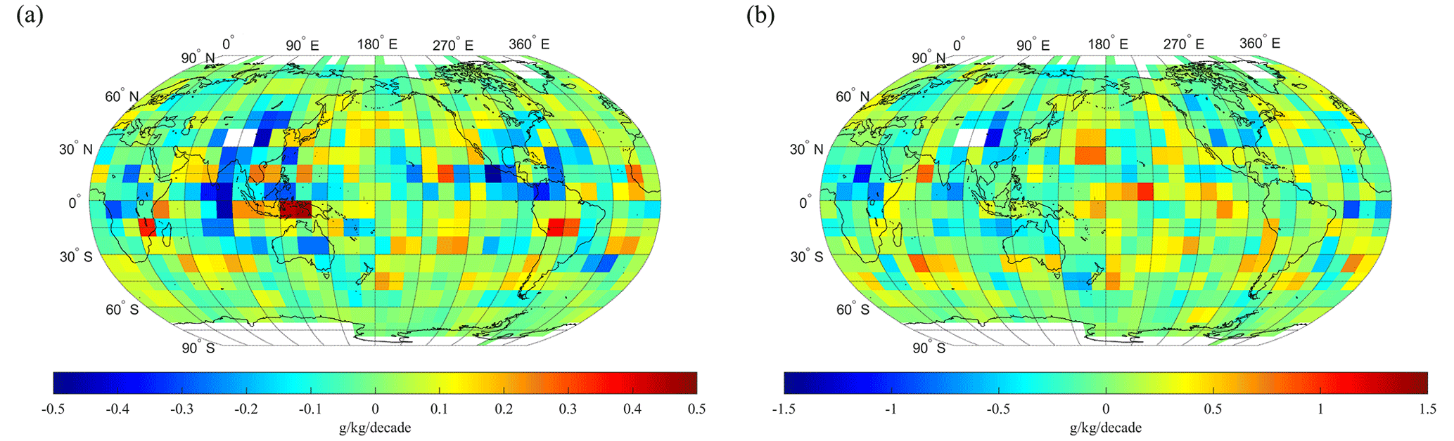
Figure A5(a, b) The distribution of trends of sampling error QSE time series at 500 and 850 hPa, respectively. The white blanks in (a) and (b) are grids with > 1.5 % missing monthly data over the 2007 to 2018 interval.
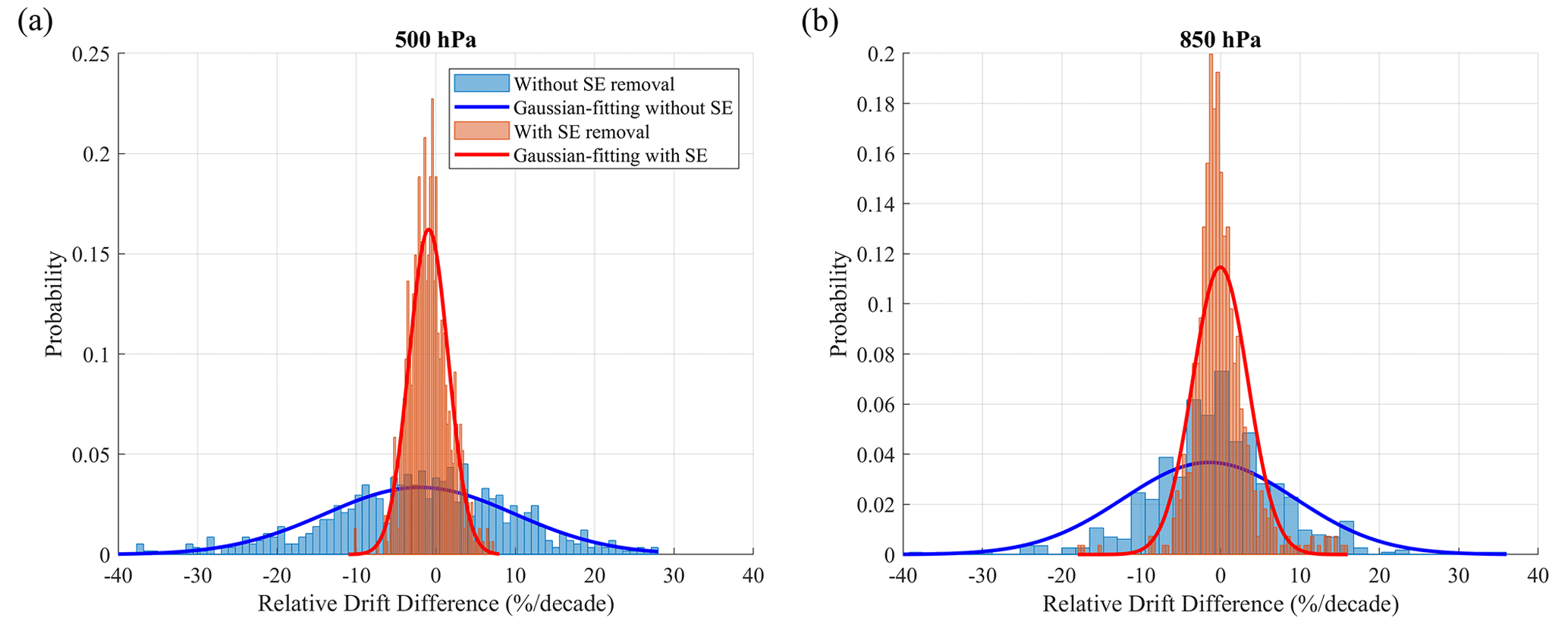
Figure A6(a, b) The histogram of relative water vapor trend difference (% per decade) between COSMIC and ERA5 water vapor at 500 and 850 hPa, respectively. In both panels, blue and orange bar charts are the distribution of the COSMIC water vapor trend difference relative to ERA5 before and after the sampling error removal was applied, respectively. The blue and red lines are the Gaussian-fitted distribution of the relative water vapor trend difference for the FWHM calculation.
A4 Comparison of COSMIC and ERA5 over sites with notable increasing and decreasing water vapor trends
Although the global and latitudinal water vapor trends presented in Sect. 4 exhibit an overall upward trend, Fig. 7a–d in Sect. 5.1 highlight that within tropical and subtropical regions, the regional distribution of water vapor trends displays significant local variations with a blend of pronounced increases and decreases in trends. Such variations in regional water vapor trends in general agree with past studies (e.g., Ross and Elliott, 2001; Dai, 2006; Mieruch et al., 2008, 2014; Zhang et al., 2018). In this section, we quantitatively evaluate the regional variability of water vapor trends by selecting a few sites with notable increasing (site nos. 8–12 in Fig. 8) and decreasing (site nos. 13–17 in Fig. 8) water vapor trends and compare with past studies. To identify these sites, we first searched the 10∘ × 10∘ global grids and identified the regions with the largest increasing and decreasing water vapor trends. Within these regions, we selected one representative 10∘ × 10∘ grid in each region as the site of interest, and the water vapor trends of these sites estimated from COSMIC and ERA5 data are listed and compared in Tables A1 and A2.
Both COSMIC and ERA5 trend data show increasing water vapor trends at 500 and 850 hPa for the five selected sites (Table A1). Sites no. 8, no. 9, and no. 12 are located in the ocean, and sites no. 10 and no. 11 are located on land. Sites no. 8, no. 9, and no. 11 have high mean water vapor (> 7.5 g kg−1 at 850 hPa and > ∼ 1.5 g kg−1 at 500 hPa). At 850 hPa, the mean water vapor from COSMIC is lower than ERA5 for all five sites in Table A1. The trends between COSMIC and ERA5 are consistent with < 2.7 % per decade at 850 hPa for these five sites. Site no. 10 (latitude: 30 to 40∘; longitude: 270 to 280∘) over land in the United States has the strongest increasing water vapor trend: > 18 % per decade at 850 hPa and > 39 % per decade at 500 hPa among all of the 10∘ by 10∘ grids over land. Site no. 10 in the United States and site no. 11 in southeastern China are representative land sites becoming moister. Among the sites situated over the ocean, sites no. 8 and no. 12 stand out with substantial increasing water vapor trends (> 17 % per decade and > 23 % per decade at 850 hPa, respectively). Many previous studies have explored the trends in surface temperature (e.g., Gu and Adler, 2022, and references therein). The global surface keeps warming up, though with rich spatial structures of temperature change. Higher surface temperatures are closely linked to higher levels of water vapor in the atmosphere through the relationship governed by the Clausius–Clapeyron equation. The saturation vapor pressure of water vapor increases with temperature. The close relations between higher temperature and higher water vapor have been shown in observations and models (Wentz and Schabel, 2000; Trenberth et al., 2005; Held and Soden, 2006; Allan et al., 2014). From the study by Gu and Adler (2022), ocean surface warming can readily be seen in the Indian and tropical Pacific oceans, roughly corresponding to the strongly increasing tropospheric water vapor trends for sites no. 8, no. 9, and no. 12 we observed.
Table A2 lists the water vapor trends for five sites with notable decreasing trends. Sites no. 13 and no. 14 are located over the ocean, and sites no. 15, no. 16, and no. 17 are located over land. For the two ocean sites, water vapor trends at 500 and 850 hPa from COSMIC and ERA5 are strongly negative (mostly < −10 % per decade). These two ocean sites accompany the regions with strong positive water vapor trends over the equatorial Pacific Ocean and the Laccadive Sea, respectively (Fig. 7). The long-term negative water vapor trend at 850 hPa for site no. 15 in southern Africa can cause a regional drier atmosphere. Site no. 16 in Brazil has a mild decreasing water vapor trend at 850 hPa and a strong decreasing water vapor trend (< −10 % per decade) at 500 hPa from COSMIC data. Site no. 17 in Australia has the lowest mean water vapor, i.e., driest, among the five sites and a strong decreasing trend (< −10 % per decade at 850 hPa), which can result in a long-term drier atmosphere in this region (Dai et al., 2006; Zhang et al., 2018). Site no. 17 is a representative dry region over land, which becomes drier at 850 hPa.
Table A1Water vapor trends over selected sites with notable increasing trends.
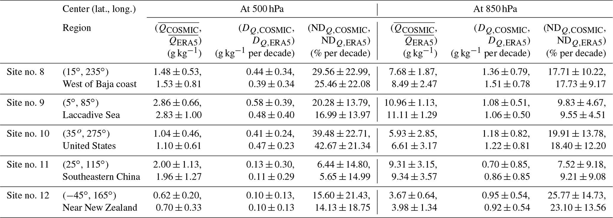
Table A2Water vapor trends over selected sites with notable decreasing trends.
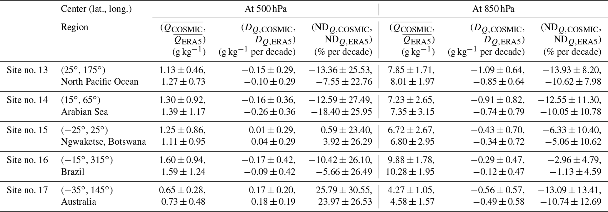
The ECMWF Reanalysis Model 5 (ERA5) data are publicly available at https://www.ecmwf.int/en/forecasts/dataset/ecmwf-reanalysis-v5 (Copernicus Climate Change Service, 2023). The UCAR COSMIC water vapor data are available at https://cdaac-www.cosmic.ucar.edu/cdaac/products.html (CDAAC, 2023).
Conceptualization by SPH and XS. XS, SPH, XZ, and YC defined the validation methodology. XJ, TCL, XS, and BZ wrote the scripts used for the analysis. XJ, TCL, XS, BZ, and JD performed the data analysis and validation. XZ, BZ, and JD provided the satellite data. XS and SPH wrote the paper. XS, SPH, XZ, YC, TCL, BZ, and JD reviewed and edited the paper. Project administration by XS and BZ. Funding acquisition by SPH and YC. All authors have read and agreed to the published version of the paper.
The contact author has declared that none of the authors has any competing interests.
The manuscript contents are solely the opinions of the authors and do not constitute a statement of policy, decision, or position on behalf of NOAA or the U.S. government.
Publisher's note: Copernicus Publications remains neutral with regard to jurisdictional claims made in the text, published maps, institutional affiliations, or any other geographical representation in this paper. While Copernicus Publications makes every effort to include appropriate place names, the final responsibility lies with the authors.
This article is part of the special issue “Analysis of atmospheric water vapour observations and their uncertainties for climate applications (ACP/AMT/ESSD/HESS inter-journal SI)”. It is not associated with a conference.
The authors would like to thank Guojun Gu, Yun Zhou, and Loknath Adhikari for their input during the process of preparing this paper.
This study was supported by NOAA grant NA19NES4320002 (Cooperative Institute for Satellite Earth System Studies – CISESS) at the University of Maryland/ESSIC.
This paper was edited by Jayanarayanan Kuttippurath and reviewed by one anonymous referee.
Adler, R. F., Gu, G., Wang, J. J., Huffman, G. J., Curtis, S., and Bolvin, D.: Relationships between global precipitation and surface temperature on interannual and longer timescales (1979–2006), J. Geophys. Res.-Atmos., 113, D22104, https://doi.org/10.1029/2008JD010536, 2008.
Ahrens, C. and Samson, P.: Extreme Weather and Climate, 1st ed., Brooks Cole, United States of America, ISBN 9781111780241, 2011.
Allan, R. P.: Analysis of moisture variability in the European Centre for Medium-Range Weather Forecasts 15-year reanalysis over the tropical oceans, J. Geophys. Res., 107, 4230, https://doi.org/10.1029/2001JD001132, 2002.
Allan, R. P. and Liepert, B. G.: Anticipated changes in the global atmospheric water cycle, Environ. Res. Lett., 5, 025201, https://doi.org/10.1088/1748-9326/5/2/025201, 2010.
Allan, R. P. and Soden, B. J.: Atmospheric warming and the amplification of precipitation extremes, Science, 321, 1481–1484, https://doi.org/10.1126/science.1160787, 2008.
Allan, R. P., Liu, C., Zahn, M., Lavers, D. A., Koukouvagias, E., and Bodas-Salcedo, A.: Physically consistent responses of the global atmospheric hydrological cycle in models and observations, Surv. Geophys., 35, 533–552, https://doi.org/10.1007/s10712-012-9213-z, 2014.
Allan, R. P., Willett, K. M., John, V. O., and Trent, T.: Global changes in water vapor 1979–2020, J. Geophysical Res.-Atmos., 127, e2022JD036728, https://doi.org/10.1029/2022JD036728, 2022.
An, Z. S., Wu, G. X., Li, J. P., Sun, Y. B., Liu, Y. M., Zhou, W. J., Cai, Y. J., Duan, A. M., Li, L., Mao, J. Y., Cheng, H., Shi, Z. G., Tan, L. C., Yan, H., Ao, H., Chang, H., and Juan, F.: Global Monsoon Dynamics and Climate Change, Annu. Rev. Earth Pl. Sc., 43, 29–77, https://doi.org/10.1146/annurev-earth-060313-054623, 2015.
Andrisaniand, A. and Vespe, F.: Humidity profiles retrieved from GNSS Radio Occultations by a non-negative residual constrained least square error method, Front. Earth Sci., 8, 320, https://doi.org/10.3389/feart.2020.00320, 2020.
Anthes, R. A., Bernhardt, P. A., Chen, Y., Cucurull, L., Dymond, K. F., Ector, D., Healy, S. B., Ho, S. P., Hunt, D. C., Kuo, Y. H., and Liu, H.: The COSMIC/FORMOSAT-3 mission: Early results, B. Am. Meteorol. Soc., 89, 313–334, https://doi.org/10.1175/BAMS-89-3-313, 2008.
Anthes, R. A., Rocken, C. and Ying-Hwa, K.: Applications of COSMIC to meteorology and climate, Terr. Atmos. Ocean. Sci., 11, 115–156, https://doi.org/10.3319/TAO.2000.11.1.115(COSMIC), 2020.
Ao, C. O.: Effect of ducting on radio occultation measurements: An assessment based on high-resolution radiosonde soundings, Radio Sci., 42, RS2008, https://doi.org/10.1029/2006RS003485, 2007.
Ao, C. O., Meehan, T. K., Hajj, G. A., Mannucci, A. J., and Beyerle, G.: Lower-troposphere refractivity bias in GPS occultation retrievals, J. Geophys. Res., 108, 4577, https://doi.org/10.1029/2002JD003216, 2003.
Bengtsson, L.: Can climate trends be calculated from reanalysis data?, J. Geophys. Res., 109, D11111, https://doi.org/10.1029/2004JD004536, 2004.
Bock, O., Guichard, F., Janicot, S., Lafore, J. P., Bouin, M. N., and Sultan, B.: Multiscale analysis of precipitable water vapor over Africa from GPS data and ECMWF analyses, Geophys. Res. Lett., 34, L09705, https://doi.org/10.1029/2006GL028039, 2007.
Borger, C., Beirle, S., and Wagner, T.: A 16-year global climate data record of total column water vapour generated from OMI observations in the visible blue spectral range, Earth Syst. Sci. Data, 15, 3023–3049, https://doi.org/10.5194/essd-15-3023-2023, 2023.
Campos, R. M., Gramcianinov, C. B., de Camargo, R., and da Silva Dias, P. L.: Assessment and Calibration of ERA5 Severe Winds in the Atlantic Ocean Using Satellite Data, Remote Sensing, 14, 4918, https://doi.org/10.3390/rs14194918, 2022.
CDAAC: UCAR COSMIC water vapor data, https://cdaac-www.cosmic.ucar.edu/cdaac/products.html (last access: 7 November 2023), CDAAC [data set], 2023.
Chen, B. and Liu, Z.: Global water vapor variability and trend from the latest 36 year (1979 to 2014) data of ECMWF and NCEP reanalyses, radiosonde, GPS, and microwave satellite, J. Geophys. Res.-Atmos., 121, 11–442, https://doi.org/10.1002/2016JD024917, 2016.
Chen, Y., Shao, X., Cao, C., and Ho, S.-P.: Simultaneous Radio Occultation Predictions for Inter-Satellite Comparison of Bending Angle Profiles from COSMIC-2 and GeoOptics, Remote Sensing, 13, 3644, https://doi.org/10.3390/rs13183644, 2021.
Chen, Y., Cao, C., Shao, X., and Ho, S.-P.: Assessment of the Consistency and Stability of CrIS Infrared Observations Using COSMIC-2 Radio Occultation Data over Ocean, Remote Sensing, 14, 2721, https://doi.org/10.3390/rs14112721, 2022.
Chou, C. and Neelin, J. D.: Mechanisms of global warming impacts on regional tropical precipitation, J. Climate, 17, 2688–2701, https://doi.org/10.1175/JCLI-D-11-00239.1, 2004.
Dai, A.: Recent climatology, variability, and trends in global surface humidity, J. Climate, 19, 3589–3606, https://doi.org/10.1175/JCLI3816.1, 2006.
Copernicus Climate Change Service: ECMWF ReAnalysis Model 5 (ERA5) data, https://www.ecmwf.int/en/forecasts/dataset/ecmwf-reanalysis-v5 (last access: 7 November 2023), Copernicus Climate Change Service [data set], 2023.
De Deckker, P.: The Indo-Pacific Warm Pool: critical to world oceanography and world climate, Geosci. Lett., 3, 1–12, https://doi.org/10.1186/s40562-016-0054-3, 2016.
Feulner, G., Rahmstorf, S., Levermann, A., and Volkwardt, S.: On the Origin of the Surface Air Temperature Difference between the Hemispheres in Earth's Present-Day Climate, J. Climate, 26, 7136–7150, https://doi.org/10.1175/JCLI-D-12-00636.1, 2013.
Forster, P., Ramaswamy, V., Artaxo, P., Berntsen, T., Betts, R., Fahey, D. W., Haywood, J., Lean, J., Lowe, D. C., Myhre, G., Nganga, J., Prinn, R., Raga, G., Schulz, M., Van Dorland, R., and Miller, H. L.: Changes in Atmospheric Constituents and in Radiative Forcing, in: Climate Change 2007: The Physical Science Basis, Contribution of working group I to the Fourth Assessment Report of the Intergovernmental Panel on Climate Change, edited by: Solomon, S., Qin, D., Manning, M., Chen, Z., Marquis, M., Averyt, K. B., Tignor, M., and Miller, H. L., Cambridge University Press, Cambridge, United Kingdom and New York, NY, USA, 2007.
Fujiwara, M., Wright, J. S., Manney, G. L., Gray, L. J., Anstey, J., Birner, T., Davis, S., Gerber, E. P., Harvey, V. L., Hegglin, M. I., Homeyer, C. R., Knox, J. A., Krüger, K., Lambert, A., Long, C. S., Martineau, P., Molod, A., Monge-Sanz, B. M., Santee, M. L., Tegtmeier, S., Chabrillat, S., Tan, D. G. H., Jackson, D. R., Polavarapu, S., Compo, G. P., Dragani, R., Ebisuzaki, W., Harada, Y., Kobayashi, C., McCarty, W., Onogi, K., Pawson, S., Simmons, A., Wargan, K., Whitaker, J. S., and Zou, C.-Z.: Introduction to the SPARC Reanalysis Intercomparison Project (S-RIP) and overview of the reanalysis systems, Atmos. Chem. Phys., 17, 1417–1452, https://doi.org/10.5194/acp-17-1417-2017, 2017.
Gleisner, H., Lauritsen, K. B., Nielsen, J. K., and Syndergaard, S.: Evaluation of the 15-year ROM SAF monthly mean GPS radio occultation climate data record, Atmos. Meas. Tech., 13, 3081–3098, https://doi.org/10.5194/amt-13-3081-2020, 2020.
Gleisner, H., Ringer, M. A., and Healy, S. B.: Monitoring global climate change using GNSS radio occultation, npj Climate and Atmospheric Science, 5, 1–4, https://doi.org/10.1038/s41612-022-00229-7, 2022.
Grossi, M., Valks, P., Loyola, D., Aberle, B., Slijkhuis, S., Wagner, T., Beirle, S., and Lang, R.: Total column water vapour measurements from GOME-2 MetOp-A and MetOp-B, Atmos. Meas. Tech., 8, 1111–1133, https://doi.org/10.5194/amt-8-1111-2015, 2015.
Gu, G. and Adler, R. F.: Interdecadal Variability/Long-Term Changes in Global Precipitation Patterns during the Past Three Decades: Global Warming and/or Pacific Decadal Variability?, Clim. Dynam., 40, 3009–3022, https://doi.org/10.1007/s00382-012-1443-8, 2013.
Gu, G. and Adler, R. F.: Observed Variability and Trends in Global Precipitation During 1979–2020, 61, 131–150, Clim. Dynam., https://doi.org/10.1007/s00382-022-06567-9, 2022.
He, J., Brogniez, H., and Picon, L.: Evaluation of tropical water vapour from CMIP6 global climate models using the ESA CCI Water Vapour climate data records, Atmos. Chem. Phys., 22, 12591–12606, https://doi.org/10.5194/acp-22-12591-2022, 2022.
Held, I. M. and Soden, B. J.: Water vapor feedback and global warming, Annu. Rev. Energ. Environ., 25, 441–475, https://doi.org/10.1146/annurev.energy.25.1.441, 2000.
Held, I. M. and Soden, B. J.: Robust responses of the hydrological cycle to global warming, J. Climate, 19, 5686–5699, https://doi.org/10.1175/JCLI3990.1, 2006.
Hegerl, G. C., Black, E., Allan, R. P., Ingram, W. J., Polson, D., Trenberth, K. E., Chadwick, R. S., Arkin, P. A., Sarojini, B. B., Becker, A., and Dai, A.: Challenges in quantifying changes in the global water cycle, B. Am. Meteorol. Soc., 96, 1097–1115, https://doi.org/10.1175/BAMS-D-13-00212.1, 2015.
Held, I. M. and Soden, B. J.: Robust Responses of the Hydrological Cycle to Global Warming, J. Climate, 19, 5686–5699, https://doi.org/10.1175/JCLI3990.1, 2006.
Hersbach, H., Bell, B., Berrisford, P., Hirahara, S., Horányi, A., Muñoz-Sabater, J., Nicolas, J., Peubey, C., Radu, R., Schepers, D., and Simmons, A.: The ERA5 global reanalysis, Q. J. Roy. Meteorol. Soc., 146, 1999–2049, https://doi.org/10.1002/qj.3803, 2020.
Ho, S. P., Kirchengast, G., Leroy, S., Wickert, J., Mannucci, A. J., Steiner, A., Hunt, D., Schreiner, W., Sokolovskiy, S., Ao, C., and Borsche, M.: Estimating the uncertainty of using GPS radio occultation data for climate monitoring: Intercomparison of CHAMP refractivity climate records from 2002 to 2006 from different data centers, J. Geophys. Res.-Atmos., 114, D23107, https://doi.org/10.1029/2009JD011969, 2009.
Ho, S. P., Zhou, X., Kuo, Y. H., Hunt, D., and Wang, J. H.: Global evaluation of radiosonde water vapor systematic biases using GPS radio occultation from COSMIC and ECMWF analysis, Remote Sensing, 2, 1320–1330, https://doi.org/10.3390/rs2051320, 2010.
Ho, S.-P., Peng, L., Anthes, R. A., Kuo, Y.-H., and Lin, H.-C.: Marine boundary layer heights and their longitudinal, diurnal, and interseasonal variability in the southeastern Pacific using COSMIC, CALIOP, and radiosonde data, J. Climate, 28, 2856–2872, https://doi.org/10.1175/JCLI-D-14-00238.1, 2015.
Ho, S.-P., Peng, L., Mears, C., and Anthes, R. A.: Comparison of global observations and trends of total precipitable water derived from microwave radiometers and COSMIC radio occultation from 2006 to 2013, Atmos. Chem. Phys., 18, 259–274, https://doi.org/10.5194/acp-18-259-2018, 2018.
Ho, S. P., Anthes, R. A., Ao, C. O., Healy, S., Horanyi, A., Hunt, D., Mannucci, A. J., Pedatella, N., Randel, W. J., Simmons, A., and Steiner, A.: The COSMIC/FORMOSAT-3 radio occultation mission after 12 years: Accomplishments, remaining challenges, and potential impacts of COSMIC-2, B. Am. Meteorol. Soc., 101, E1107–E1136, https://doi.org/10.1175/BAMS-D-18-0290.1, 2020a.
Ho, S. P., Zhou, X., Shao, X., Zhang, B., Adhikari, L., Kireev, S., He, Y., Yoe, J. G., Xia-Serafino, W., and Lynch, E.: Initial assessment of the COSMIC-2/FORMOSAT-7 neutral atmosphere data quality in NESDIS/STAR using in situ and satellite data, Remote Sensing, 12, 4099, https://doi.org/10.3390/rs12244099, 2020b.
Ho, S.-p., Kireev, S., Shao, X., Zhou, X., and Jing, X.: Processing and Validation of the STAR COSMIC-2 Temperature and Water Vapor Profiles in the Neutral Atmosphere, Remote Sensing, 14, 5588, https://doi.org/10.3390/rs14215588, 2022.
Huang, C. Y., Teng, W. H., Ho, S. P., and Kuo, Y. H.: Global variation of COSMIC precipitable water over land: Comparisons with ground-based GPS measurements and NCEP reanalyses, Geophys. Res. Lett., 40, 5327–5331, https://doi.org/10.1002/grl.50885, 2013.
Iacovazzi, R., Lin, L., Sun, N., and Liu, Q.: NOAA operational microwave sounding radiometer data quality monitoring and anomaly assessment using COSMIC GNSS radio-occultation soundings, Remote Sensing, 12, 828, https://doi.org/10.3390/rs12050828, 2020.
Johnston, B. R., Randel, W. J., and Sjoberg J. P.: Evaluation of Tropospheric Moisture Characteristics Among COSMIC-2, ERA5 and MERRA-2 in the Tropics and Subtropics, Remote Sensing, 13, 880, https://doi.org/10.3390/rs13050880, 2021.
Johnston, B. R., Randel, W. J., and Braun, J. J.: Interannual Variability of Tropospheric Moisture and Temperature and Relationships to ENSO Using COSMIC-1 GNSS-RO Retrievals, J. Climate, 35, 3509–3525, https://doi.org/10.1175/JCLI-D-21-0884.1, 2022.
Kiehl, J. T. and Trenberth, K. E.: Earth's annual global mean energy budget, B. Am. Meteorol. Soc., 78, 197–208, https://doi.org/10.1175/1520-0477(1997)078<0197:EAGMEB>2.0.CO;2, 1997.
Krüger, K., Schäfler, A., Wirth, M., Weissmann, M., and Craig, G. C.: Vertical structure of the lower-stratospheric moist bias in the ERA5 reanalysis and its connection to mixing processes, Atmos. Chem. Phys., 22, 15559–15577, https://doi.org/10.5194/acp-22-15559-2022, 2022.
Kursinski, E. R. and Hajj, G. A.: A comparison of water vapor derived from GPS occultations and global weather analyses, J. Geophys. Res., 106, 1113–1138, https://doi.org/10.1029/2000JD900421, 2021.
Kursinski, E. R., Hajj, G. A., Schofield, J. T., Linfield, R. P., and Hardy, K. R.: Observing Earth's atmosphere with radio occultation measurements using the Global Positioning System, J. Geophys. Res.-Atmos., 102, 23429–23465, https://doi.org/10.1029/97JD01569, 1997.
Lei, Y., Letu, H., Shang, H., and Shi, J.: Cloud cover over the Tibetan Plateau and eastern China: a comparison of ERA5 and ERA-Interim with satellite observations, Clim. Dynam., 54, 2941–2957, https://doi.org/10.1007/s00382-020-05149-x, 2020.
Lonitz, K. and Geer, A.: Effect of assimilating microwave imager observations in the presence of a model bias in marine stratocumulus, EUMETSAT/ECMWF Fellowship Programme Research Reports, https://www.ecmwf.int/node/17164 (last access: 7 November 2023), 2017.
Lu, N., Qin, J., Gao, Y., Yang, K., Trenberth, K. E., Gehne, M. and Zhu, Y.: Trends and variability in atmospheric precipitable water over the Tibetan Plateau for 2000–2010, Int. J. Climatol., 35, 1394–1404, https://doi.org/10.1002/joc.4064, 2015.
Mears, C., Ho, S. P., Wang, J., Huelsing, H., and Peng, L.: Total column water vapor [in “States of the Climate in 2016”], B. Am. Meteorol. Soc., 98, S24–S25, https://doi.org/10.1175/2017BAMSStateoftheClimate.1, 2017.
Mears, C., Ho, S.-P., Zhang, L., and Zhou, X.: Total Column Water Vapor section, in: States of the Climate in 2021, edited by: Blunden, J. and Boyer, T., B. Am. Meteorol. Soc., 103, 52–56, https://doi.org/10.1175/2022BAMSStateoftheClimate.1, 2022.
Mieruch, S., Noël, S., Bovensmann, H., and Burrows, J. P.: Analysis of global water vapour trends from satellite measurements in the visible spectral range, Atmos. Chem. Phys., 8, 491–504, https://doi.org/10.5194/acp-8-491-2008, 2008.
Mieruch, S., Schröder, M., Noël, S., and Schulz, J., Comparison of decadal global water vapor changes derived from independent satellite time series, J. Geophys. Res.-Atmos., 119, 12489–12499, https://doi.org/10.1002/2014JD021588, 2014.
Nilsson, T. and Elgered, G.: Long-term trends in the atmospheric water vapor content estimated from ground-based GPS data, J. Geophys. Res.-Atmos., 113, https://doi.org/10.1029/2008JD010110, 2008.
Parker, D., Folland, C., Scaife, A., Knight, J., Colman, A., Baines, P., and Dong, B.: Decadal to multidecadal variability and the climate change background, J. Geophys. Res.-Atmos., 112, D18115, https://doi.org/10.1029/2007JD008411, 2007.
Patel, V. and Kuttippurath, J.: Significant increase in water vapour over India and Indian Ocean: Implications for tropospheric warming and regional climate forcing, Sci. Total Environ., 838, 155885, https://doi.org/10.1016/j.scitotenv.2022.155885, 2022.
Rosenkranz, P. W.: Retrieval of temperature and moisture profiles from AMSU-A and AMSU-B measurements, IEEE T. Geosci. Remote, 39, 2429–2435, https://doi.org/10.1109/36.964979, 2001.
Ross, R. J. and Elliott, W. P.: Radiosonde-based Northern Hemisphere tropospheric water vapor trends, J. Climate, 14, 1602–1612, https://doi.org/10.1175/1520-0442(2001)014<1602:RBNHTW>2.0.CO;2, 2001.
Santer, B. D., Wigley, T. M. L., Gleckler, P. J., Bonfils, C., Wehner, M. F., AchutaRao, K., Barnett, T. P., Boyle, J. S., Brüggemann, W., Fiorino, M., and Gillett, N.: Forced and unforced ocean temperature changes in Atlantic and Pacific tropical cyclogenesis regions, P. Natl. Acad. Sci. USA, 103, 13905–13910, https://doi.org/10.1073/pnas.0602861103, 2006.
Sherwood, S. C., Roca, R., Weckwerth, T. M., and Andronova, N. G.: Tropospheric water vapor, convection, and climate, Rev. Geophys., 48, RG2001, https://doi.org/10.1029/2009RG000301, 2010.
Shao, X., Ho, S. P., Zhang, B., Cao, C., and Chen, Y.: Consistency and Stability of SNPP ATMS Microwave Observations and COSMIC-2 Radio Occultation over Oceans, Remote Sensing, 13, 3754, https://doi.org/10.3390/rs13183754, 2021a.
Shao, X., Ho, S. P., Zhang, B., Zhou, X., Kireev, S., Chen, Y., and Cao, C.: Comparison of COSMIC-2 radio occultation retrievals with RS41 and RS92 radiosonde humidity and temperature measurements, Terr. Atmos. Ocean. Sci., 32, 1015–1032, https://doi.org/10.3319/TAO.2021.12.30.02, 2021b.
Shen, Z., Zhang, K., He, Q., Wan, M., Li, L., and Wu, S.: Quest over the Sampling Error of COSMIC Radio Occultation Temperature Climatologies, J. Atmos. Ocean. Tech., 38, 441–458, https://doi.org/10.1175/JTECH-D-19-0169.1, 2021.
Sokolovskiy, S.: Effect of superrefraction on inversions of radio occultation signals in the lower troposphere, Radio Sci., 38, 1058, https://doi.org/10.1029/2002RS002728, 2003.
Smith, T. M. and Reynolds, R. W.: A global merged land–air–sea surface temperature reconstruction based on historical observations (1880–1997), J. Climate, 18, 2021–2036, https://doi.org/10.1175/JCLI3362.1, 2005.
Sun, B., Reale, T., Schroeder, S., Pettey, M. and Smith, R.: On the accuracy of Vaisala RS41 versus RS92 upper-air temperature observations, J. Atmos. Ocean. Techn., 36, 635–653, https://doi.org/10.1175/JTECH-D-18-0081.1, 2019.
Susskind, J., Barnet, C., and Blaisdell, J.: Retrieval of atmospheric and surface parameters from AIRS/AMSU/HSB data in the presence of clouds, IEEE T. Geosci. Remote, 41, 390–409, https://doi.org/10.1109/TGRS.2002.808236, 2003.
Tang, W., Qin, J., Yang, K., Zhu, F., and Zhou, X.: Does ERA5 outperform satellite products in estimating atmospheric downward longwave radiation at the surface?, Atmos. Res., 252, 105453, https://doi.org/10.1016/j.atmosres.2021.105453, 2021.
Trenberth, K. E.: Changes in precipitation with climate change, Clim. Res., 47, 123–138, https://doi.org/10.3354/cr00953, 2011.
Trenberth, K. E., Fasullo, J., and Smith, J.: Trends and variability in column-integrated atmospheric water vapor, Clim. Dynam., 24, 741–758, https://doi.org/10.1007/s00382-005-0017-4, 2005.
Turner, A. G. and Annamalai, H.: Climate change and the South Asian summer monsoon, Nat. Clim. Change, 2, 587–595, https://doi.org/10.1038/nclimate1495, 2012.
Vey, S., Dietrich, R., Rülke, A., Fritsche, M., Steigenberger, P., and Rothacher, M.: Validation of precipitable water vapor within the NCEP/DOE Reanalysis using global GPS observations from one decade, J. Climate, 23, 1675–1695, https://doi.org/10.1175/2009JCLI2787.1, 2010.
Wagner, T., Beirle, S., Grzegorski, M., and Platt, U.: Global trends (1996–2003) of total column precipitable water observed by Global Ozone Monitoring Experiment (GOME) on ERS-2 and their relation to near-surface temperature, J. Geophys. Res., 111, D12102, https://doi.org/10.1029/2005JD006523, 2006.
Wang, R., Fu, Y., Xian, T., Chen, F., Yuan, R., Li, R., and Liu, G.: Evaluation of atmospheric precipitable water characteristics and trends in mainland China from 1995 to 2012, J. Climate, 30, 8673–8688, https://doi.org/10.1175/JCLI-D-16-0433.1, 2017.
Wee, T.-K., Anthes, R. A., Hunt, D. C., Schreiner, W. S., and Kuo, Y.-H.: Atmospheric GNSS RO 1D-Var in Use at UCAR: Description and Validation, Remote Sens., 14, 5614, https://doi.org/10.3390/rs14215614, 2022.
Wentz, F. J. and Schabel, M.: Precise climate monitoring using complementary satellite data sets, Nature, 403, 414–416, https://doi.org/10.1038/35000184, 2000.
Whitaker, J. S., Hamill, T. M., Wei, X., Song, Y., and Toth, Z.: Ensemble Data Assimilation with the NCEP Global Forecast System, Mon. Weather Rev., 136, 463–482, https://doi.org/10.1175/2007MWR2018.1, 2008.
Wood, R.: Stratocumulus clouds, Mon. Weather Rev., 140, 2373–2423, https://doi.org/10.1175/MWR-D-11-00121.1, 2012.
Wood, R., Mechoso, C. R., Bretherton, C. S., Weller, R. A., Huebert, B., Straneo, F., Albrecht, B. A., Coe, H., Allen, G., Vaughan, G., Daum, P., Fairall, C., Chand, D., Gallardo Klenner, L., Garreaud, R., Grados, C., Covert, D. S., Bates, T. S., Krejci, R., Russell, L. M., de Szoeke, S., Brewer, A., Yuter, S. E., Springston, S. R., Chaigneau, A., Toniazzo, T., Minnis, P., Palikonda, R., Abel, S. J., Brown, W. O. J., Williams, S., Fochesatto, J., Brioude, J., and Bower, K. N.: The VAMOS Ocean-Cloud-Atmosphere-Land Study Regional Experiment (VOCALS-REx): goals, platforms, and field operations, Atmos. Chem. Phys., 11, 627–654, https://doi.org/10.5194/acp-11-627-2011, 2011.
Xie, F., Syndergaard, S., Kursinski, E. R., and Herman, B. M.: An Approach for Retrieving Marine Boundary Layer Refractivity from GPS Occultation Data in the Presence of Superrefraction, J. Atmos. Ocean. Tech., 23, 1629–1644, https://doi.org/10.1175/jtech1996.1, 2006.
Xie, F., Wu, D. L., Ao, C. O., Kursinski, E. R., Mannucci, A. J., and Syndergaard, S.: Super-refraction effects on GPS radio occultation refractivity in marine boundary layers, Geophys. Res. Lett., 37, L11805, https://doi.org/10.1029/2010gl043299, 2010.
Xie, F., Tian, W., Zhou, X., Zhang, J., Xia, Y., and Lu, J.: Increase in lower stratospheric water vapor in the past 100 years related to tropical Atlantic warming, Geophys. Res. Lett., 47, e2020GL090539, https://doi.org/10.1029/2020GL090539, 2020.
Yadav, R., Giri, R. K., and Singh, V.: Intercomparison review of IPWV retrieved from INSAT-3DR sounder, GNSS and CAMS reanalysis data, Atmos. Meas. Tech., 14, 4857–4877, https://doi.org/10.5194/amt-14-4857-2021, 2021.
Yuan, P., Van Malderen, R., Yin, X., Vogelmann, H., Jiang, W., Awange, J., Heck, B., and Kutterer, H.: Characterisations of Europe's integrated water vapour and assessments of atmospheric reanalyses using more than 2 decades of ground-based GPS, Atmos. Chem. Phys., 23, 3517–3541, https://doi.org/10.5194/acp-23-3517-2023, 2023.
Zhai, P. and Eskridge, R. E.: Atmospheric water vapor over China, J. Climate, 10, 2643–2652, https://doi.org/10.1175/1520-0442(1997)010<2643:AWVOC>2.0.CO;2, 1997.
Zhang, L., Wu, L., and Gan, B.: Modes and mechanisms of global water vapor variability over the twentieth century, J. Climate, 26, 5578–5593, https://doi.org/10.1175/JCLI-D-12-00585.1, 2013.
Zhang, Y., Xu, J., Yang, N., and Lan, P.: Variability and trends in global precipitable water vapor retrieved from COSMIC radio occultation and radiosonde observations, Atmosphere, 9, 174, https://doi.org/10.3390/atmos9050174, 2018.
Zhao, T., Dai, A., and Wang, J.: Trends in tropospheric humidity from 1970 to 2008 over China from a homogenized radiosonde dataset, J. Climate, 25, 4549–4567, https://doi.org/10.1175/JCLI-D-11-00557.1, 2012.
Zveryaev, I. I. and Allan, R. P.: Water vapor variability in the tropics and its links to dynamics and precipitation, J. Geophys. Res.-Atmos., 110, D21112, https://doi.org/10.1029/2005JD006033, 2005.
- Abstract
- Introduction
- Datasets used for spatial and temporal water vapor variability analysis
- Comparison of spatial variability of water vapor between COSMIC and ERA5
- COSMIC and ERA5 water vapor time series analysis and trend comparison
- Regional comparisons of COSMIC and ERA5 water vapor trends
- Discussion and conclusion
- Appendix A
- Data availability
- Author contributions
- Competing interests
- Disclaimer
- Special issue statement
- Acknowledgements
- Financial support
- Review statement
- References