the Creative Commons Attribution 4.0 License.
the Creative Commons Attribution 4.0 License.
 | 08 Nov 2023
Biomass-burning smoke's properties and its interactions with marine stratocumulus clouds in WRF-CAM5 and southeastern Atlantic field campaigns
Pablo E. Saide
Amie Dobracki
Steffen Freitag
Jim M. Haywood
Steven G. Howell
Siddhant Gupta
Janek Uin
Mary Kacarab
Chongai Kuang
L. Ruby Leung
Athanasios Nenes
Greg M. McFarquhar
James Podolske
Jens Redemann
Arthur J. Sedlacek
Kenneth L. Thornhill
Jenny P. S. Wong
Robert Wood
Huihui Wu
Yang Zhang
Jianhao Zhang
Paquita Zuidema
A large part of the uncertainty in climate projections comes from uncertain aerosol properties and aerosol–cloud interactions as well as the difficulty in remotely sensing them. The southeastern Atlantic functions as a natural laboratory to study biomass-burning smoke and to constrain this uncertainty. We address these gaps by comparing the Weather Research and Forecasting with Chemistry Community Atmosphere Model (WRF-CAM5) to the multi-campaign observations ORACLES (ObseRvations of Aerosols above CLouds and their intEractionS), CLARIFY (CLoud–Aerosol–Radiation Interaction and Forcing), and LASIC (Layered Atlantic Smoke Interactions with Clouds) in the southeastern Atlantic in August 2017 to evaluate a large range of the model's aerosol chemical properties, size distributions, processes, and transport, as well as aerosol–cloud interactions. Overall, while WRF-CAM5 is able to represent smoke properties and transport, some key discrepancies highlight the need for further analysis. Observations of smoke composition show an overall decrease in aerosol mean diameter as smoke ages over 4–12 d, while the model lacks this trend. A decrease in the mass ratio of organic aerosol (OA) to black carbon (BC), OA:BC, and the OA mass to carbon monoxide (CO) mixing ratio, OA:CO, suggests that the model is missing processes that selectively remove OA from the particle phase, such as photolysis and heterogeneous aerosol chemistry. A large (factor of ∼2.5) enhancement in sulfate from the free troposphere (FT) to the boundary layer (BL) in observations is not present in the model, pointing to the importance of properly representing secondary sulfate aerosol formation from marine dimethyl sulfide and gaseous SO2 smoke emissions. The model shows a persistent overprediction of aerosols in the marine boundary layer (MBL), especially for clean conditions, which multiple pieces of evidence link to weaker aerosol removal in the modeled MBL than reality. This evidence includes several model features, such as not representing observed shifts towards smaller aerosol diameters, inaccurate concentration ratios of carbon monoxide and black carbon, underprediction of heavy rain events, and little evidence of persistent biases in modeled entrainment. The average below-cloud aerosol activation fraction remains relatively constant in WRF-CAM5 between field campaigns (∼0.65), while it decreases substantially in observations from ORACLES (∼0.78) to CLARIFY (∼0.5), which could be due to the model misrepresentation of clean aerosol conditions. WRF-CAM5 also overshoots an observed upper limit on liquid cloud droplet concentration around NCLD= 400–500 cm−3 and overpredicts the spread in NCLD. This could be related to the model often drastically overestimating the strength of boundary layer vertical turbulence by up to a factor of 10. We expect these results to motivate similar evaluations of other modeling systems and promote model development to reduce critical uncertainties in climate simulations.
- Article
(6054 KB) - Full-text XML
- BibTeX
- EndNote


Among the anthropogenic radiative forcers quantified by the IPCC (Intergovernmental Panel on Climate Change), aerosols and their related cloud feedbacks have the largest uncertainty in global net radiative forcing (Bellouin et al., 2020; Boucher et al., 2013; Myhre et al., 2013). This is especially true of shallow stratocumulus clouds that top the boundary layer (Schneider et al., 2017).
Southern Africa is one of the largest regional sources of biomass-burning aerosols (BBAs) in the world, driven largely by human activities related to annual agricultural burning and land clearing during the dry season (Andela and van der Werf, 2014; Earl et al., 2015). Those emissions form large regional plumes that, depending on meteorological conditions, advect westward and interact with the expansive, bright, semi-permanent stratocumulus cloud deck off the western coast (Adebiyi and Zuidema, 2016; Garstang et al., 1996; Kaufman et al., 2003; Miller et al., 2021; Zhang and Zuidema, 2021). The complexity of aerosols and cloud behavior introduces a large source of uncertainty into aerosol radiative effects over the southeastern Atlantic (SEA) (Redemann et al., 2021; Zhang et al., 2016; Zuidema et al., 2016). These radiative effects are a product of both the smoke plume properties and the underlying cloud albedo in the SEA, wherein the latter is also influenced by microphysical aerosol–cloud interactions (Cochrane et al., 2019; Eck et al., 2013; Kaufman et al., 2003; Leahy et al., 2007; Magi et al., 2008; Waquet et al., 2013; Chand et al., 2009; Bond et al., 2013; Christensen et al., 2020; Adebiyi and Zuidema, 2018).
Aerosol–cloud interactions in the SEA can drive large regional uncertainty in radiative effects through multiple mechanisms. Absorbing aerosols in this region have been, to varying degrees, connected to changes in cloud albedo, fraction, lifetime, drizzle rate, cloud droplet size and number, and large-scale breakup or persistence (Christensen et al., 2020; Diamond et al., 2022; Yamaguchi et al., 2015, 2017; Zhang and Zuidema, 2019; Zhou et al., 2017). Therefore, constraint on both smoke representation in models, and especially aerosol–cloud interactions, is crucial to reducing uncertainties in global climate projections.
Campaigns that utilize in situ observation platforms are critical to quantifying aerosol–cloud interactions and are less vulnerable to assumptions about aerosol properties or distributions than satellite measurements (Li et al., 2020; Kaufman et al., 2003). Different models generally utilize a wide range of parameter values for aerosol physical and chemical properties such as size distribution parameters, optical properties, hygroscopic water uptake, and density (Gordon et al., 2018; Lu et al., 2018, 2021; Saide et al., 2020; Lou et al., 2020; Che et al., 2021). Additionally, models will often include representation of different aerosol aging and removal processes (Yu et al., 2019; Zawadowicz et al., 2020; Saide et al., 2012; Konovalov et al., 2019; Lou et al., 2020). The wide range of parameters and processes implemented plays a role in the uncertainties of their predictions, both of which can be constrained by field campaign data (Johnson et al., 2018).
Valuable observational constraints on these processes come from three field campaigns in this region overlapping in August 2017. ORACLES (ObseRvations of Aerosols above CLouds and their intEractionS) was a NASA aircraft campaign in 2016–2018 that studied biomass-burning smoke and clouds in the southeastern Atlantic using remote-sensing and in situ instruments (Redemann et al., 2021). CLARIFY-2017 (CLoud–Aerosol–Radiation Interaction and Forcing: Year 2017, Haywood et al., 2021) was a campaign funded by the UK's Natural Environment Research Council (NERC) centered on the UK's Facility for Airborne Atmospheric Measurements (FAAM). It was based primarily around Ascension Island (ASI) in the southeastern Atlantic and also studied physical, chemical, and radiative effects of biomass-burning smoke in this remote region. Finally, LASIC (Layered Atlantic Smoke Interactions with Clouds, Zuidema et al., 2018a) was a U.S. Department of Energy campaign that installed the Atmospheric Radiation Measurement (ARM) Mobile Facility 1 on ASI to observe the remote marine troposphere in both 2016 and 2017, covering both years' biomass-burning seasons.
Two recent analyses examined multiple models' performance against observations from ORACLES. First, compared to ORACLES observations in September 2016 (Shinozuka et al., 2020), the regional Weather Research and Forecasting with Chemistry Community Atmosphere Model version 5 (WRF-CAM5) was found to perform well among the study cohort (vs. EAM-E3SM, GEOS-5, GEOS-Chem, and the UK Unified Model (UM-UKCA), all global) compared to smoke observations. WRF-CAM5 and GEOS-5 had a finer horizontal resolution at ∼30 km, UM-UKCA was 61 km by 92 km, EAM-E3SM was 100 km, and GEOS-Chem was 2.5∘ × 2∘. All were fed by QFED2 fire emissions except UM-UKCA (FEER fires) and E3SM (GFED fires). All the models' aerosol schemes also contained the main fire emission species of interest (black carbon and organic aerosol) along with other aerosols such as sea salt, sulfate, and dust. WRF-CAM5 had the smallest error in both free-tropospheric OA and BC mass concentration and spatial distribution, although OA mass still varied widely with a root-mean-square error around 40 % in the lower free troposphere (FT). Models in this study also consistently exhibited biases towards a lower smoke layer base in the FT compared to lidar observations and plume top height differences of generally less than a model vertical grid cell. WRF-CAM5 was also found to overestimate BC in the boundary layer offshore. CO was largely underestimated, especially in the lower FT and further offshore.
WRF-CAM5 was also compared to GEOS-5, CNRM-ALADIN, and UM-UKCA with a focus on aerosol extensive and intensive properties important to the direct aerosol radiative effect (Doherty et al., 2022). This study used model output covering all three ORACLES deployments in September 2016, August 2017, and October 2018. QFED2 emissions were used in both WRF-CAM5 and GEOS-5, FEER was used in UM-UKCA, and GFED was used in ALADIN. Doherty et al. (2022) found that WRF-CAM5 had a bias towards low CO compared to observations in the core of the smoke plume (a median CO bias of −32 % to −13 %). However, WRF-CAM5 outperformed GEOS-5 and UM-UKCA in representing both BC and OA concentrations at 1–3 km above the surface in 2017, which is the focus of this study, with a WRF-CAM5 median bias in BC concentration of −20 % to +38 % and a median bias in OA concentration of −8 % to +23 % in that year compared to observations. OA and BC in WRF-CAM5 were better represented in the 1–3 km height range compared to GEOS-5 in 2016 and 2018 as well, and the WRF-CAM5 bias was similar to or lower than those of UM-UKCA in 2016 and 2017. The OA concentrations in the upper FT in both WRF-CAM5 and GEOS-5, especially between 4 and 6 km altitude, were 2–10 times higher than observations. BC from 4 to 5 km was low in both models by a factor of 2. UM-UKCA showed biases of the same sign and smaller magnitudes for both OA and BC in the 4–6 km range. ALADIN biases of these quantities were not reported. In summary, we expect that WRF-CAM5 will capture the plausible ranges of major smoke component concentrations in the year and altitudes studied here, where the largest smoke concentration and transport exist.
The first goal of this work is to analyze the performance of a fully online aerosol-resolving model, WRF-CAM5, in representing biomass-burning smoke processes. The model is compared to a wide range of observations from August 2017, when three field campaigns overlapped: ORACLES, CLARIFY-2017 (Haywood et al., 2021), and LASIC (Zuidema et al., 2018a). The second goal is to identify significant processes that may be missing or whose model representations cause substantial discrepancies between modeled and observed properties. Section 2 discusses the campaigns and data analyzed as well as the configuration of WRF-CAM5, our sampling methods, and meaningful derived quantities. Section 3 compares observations with the model-simulated smoke extensive properties such as number and mass concentrations as well as intensive properties such as size, hygroscopicity, and composition in the FT. We then address observations of changing smoke properties that suggest long-term aging and that are not captured in the model. Simulated smoke in the marine boundary layer (MBL) is also evaluated, especially utilizing observations from an ARM ground station. We further discuss aerosol composition, size distribution, hygroscopicity, and the representation of smoky and clean periods. Finally, we analyze model cloud activation and what it may reveal about the underlying process biases.
Here we evaluate a wide array of observations to understand key physical processes and judge model performance. This approach allows us to understand complex coupled processes over a much larger area than single-campaign studies typically cover. First, we introduce the array of instruments and their related data product from across the three campaigns. Second, we describe the important derived quantities from those instruments, including hygroscopicity, turbulent updrafts, BL height, and BL capping inversion strength. Third, we present notes on data usage and validation between comparable instruments. Fourth, we discuss the model build and configuration used here. Finally, we discuss the selection of data points for this analysis, including identifying smoky FT segments and cloud vertical profiles.
2.1 Observation systems
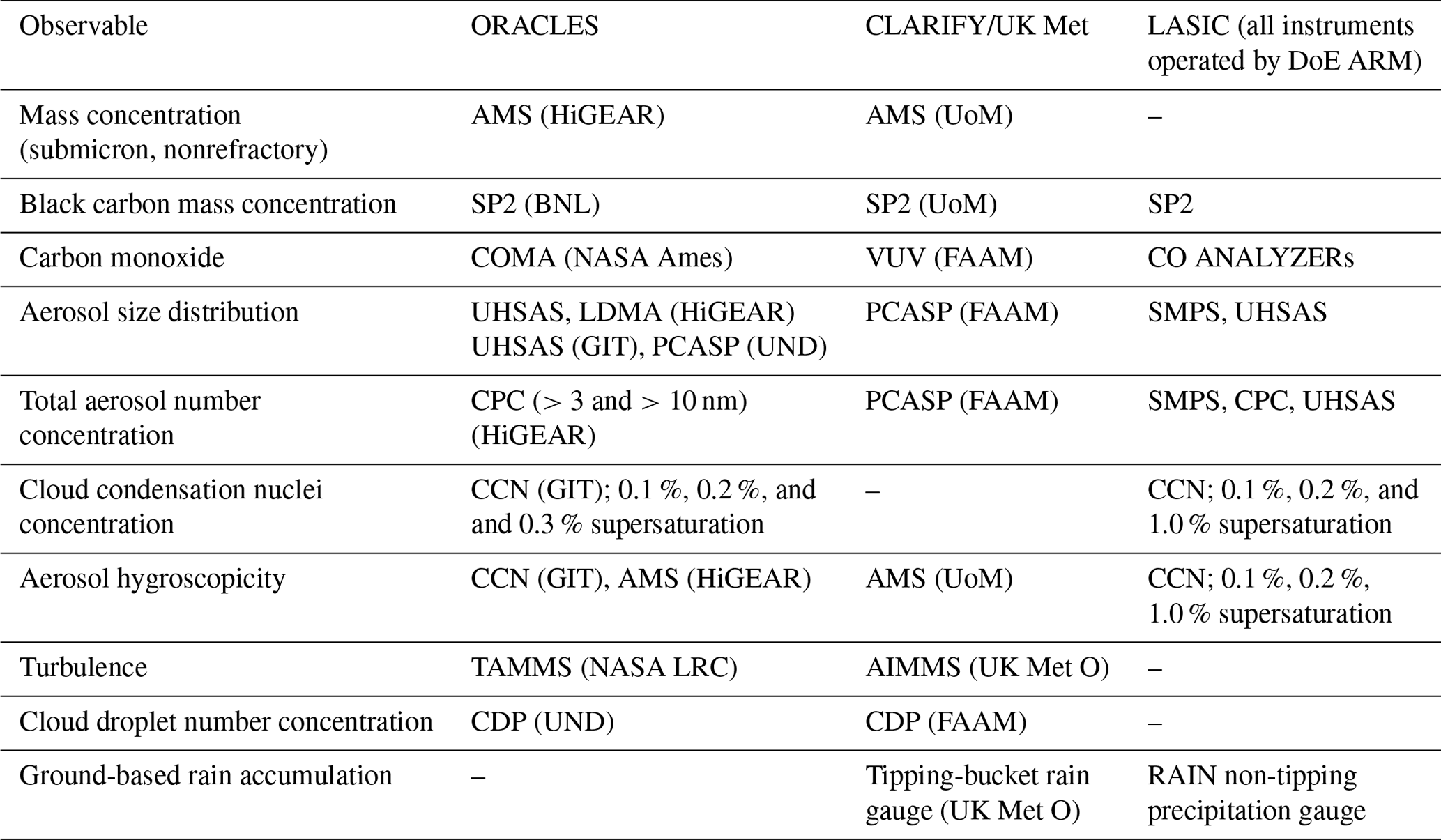
Model performance was evaluated by comparing model simulations with extensive in situ and remote-sensing data from three field campaigns in the SEA that coincided in August 2017 – ORACLES, CLARIFY-2017, and LASIC. The model domain and field campaigns are shown in Fig. 1. The ORACLES campaign consisted of flights during the biomass-burning seasons in southern Africa in 2016–2018 utilizing a mid-altitude P3 (2016–2018) and high-altitude ER2 (2016 only). The ORACLES base of operation was Walvis Bay, Namibia, in 2016 and the island of São Tomé, São Tomé and Príncipe, in 2017 and 2018. ORACLES flew various planned and opportunistic transects throughout the SEA (Redemann et al., 2021). This work uses data exclusively from the August 2017 ORACLES deployment. The CLARIFY-2017 campaign in August–September 2017 flew an instrumented Bae146 FAAM aircraft from ASI in an approximately 5∘ radius around the island to sample smoke and clouds (Haywood et al., 2021). The LASIC campaign studied aerosol, clouds, and their radiation interactions from June 2016 to October 2017, covering two biomass-burning seasons (Zuidema et al., 2016, 2018a). The data at ASI are supplemented by measurements from a permanent weather emplacement on the island, ∼5 km away from the LASIC ARM station and operated by the UK Met Office. The selected instruments used in this analysis across all three campaigns are detailed in Table 1 and are described in detail in the campaign overview papers and references therein (Zuidema et al., 2018a; Haywood et al., 2021; Taylor et al., 2020; Barrett et al., 2022; Wu et al., 2020; Redemann et al., 2021; Dobracki et al., 2023).
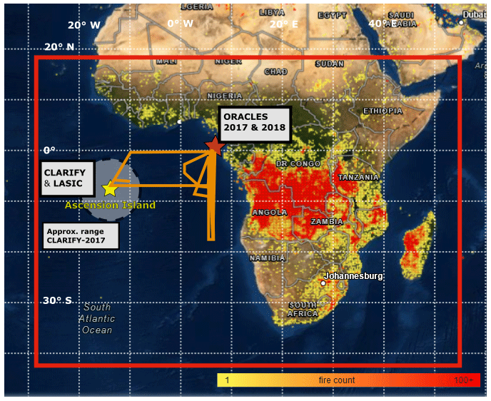
Figure 1Domain of the WRF-CAM5 run for this study (red box) and the location of each observational campaign. Orange lines represent the approximate flight tracks of ORACLES 2017 flights. Color points are regridded fire detection counts in August 2017 from VIIRS/S-NPP and a map layer obtained from NASA FIRMS.
Table 1Summary of aerosol observations from field campaigns included in this study. Groups providing observations are noted in parentheses, and the abbreviations denote the following. DoE ARM – U.S. Department of Energy Atmospheric Radiation Measurement; HiGEAR: Hawaii Group for Environmental Aerosol Research; UoM – University of Manchester; FAAM – Facility for Airborne Atmospheric Measurements; GIT – Nenes group at Georgia Institute of Technology; UND – Poellot group at the University of North Dakota; BNL – Brookhaven National Lab; LRC – NASA Langley Research Center; UK Met O – UK Met Office. Instrument abbreviations denote the following. AMS – High-resolution Time-of-Flight Aerosol Mass Spectrometer; SP2 – Single Particle Soot Photometer; COMA – Carbon mOnoxide Measurement from Ames; VUV – NCAR vacuum UV fluorometer; UHSAS – Ultra-High-Sensitivity Aerosol Spectrometer; LDMA – Long Differential Mobility Analyzer; SMPS – Scanning Mobility Particle Sizer; PCASP – Passive Cavity Aerosol Spectrometer Probe; CPC – condensation particle counter; CCN – cloud condensation nuclei; TAMMS – P3 Turbulent Air Motion Measurement System; AIMMS – Aircraft Integrated Meteorological Measurement System; CDP – Cloud Droplet Probe.
2.2 Data processing
Here we outline specific methods of deriving key quantities from observations used to evaluate the model. Single-parameter hygroscopicity is estimated using two independent methods, both of which are widely adopted and described in Petters and Kredenweis (2007). First, we use Aerosol Mass Spectrometer (AMS) chemical mass and assumed density to calculate a simple volume-weighted average hygroscopicity assuming internal mixing. We assume hygroscopicity values and density for each species in AMS and SP2 observations and the corresponding prescribed values in the model, as shown in Table 2. Second, we analyze the CCN concentration at 0.1 %, 0.2 %, and 0.3 % in combination with the aerosol size distribution to find the critical dry particle diameter of activation. For a given supersaturation (SS, the relative humidity above 100 % where particles begin deliquescing) setting, the number size distribution is integrated from large bins down to small ones, and the diameter bin at which the integrated number concentration is first greater than or equal to the CCN concentration is the critical activation diameter Dcrit. The diameter is used in the approximation formula (Petters and Kreidenweis, 2007). This equation is based on Eq. (10) in Petters and Kreidenweis (2007), takes Dcrit in nanometers, substitutes numerical values for the constants suggested, and approximates for realistic SS values of 0.1 %–1.0 %. For ORACLES, we used the GIT UHSAS, as it was configured to use the same aerosol sampling line as the CCN, as well as CCN measurements at 0.1 %, 0.2 %, and 0.3 % SS. UHSAS and CCN data are not used for 15 August 2017, as it was found that CCN counts at 0.3 % SS for that day exceeded the UHSAS count, which is not physically realistic. Number concentrations and Dcrit on the other days are within plausible ranges of count and derived κ. Kacarab et al. (2020) similarly found CCN Dcrit in the 100–200 nm range in ORACLES data, supporting this assessment. For LASIC, we use the SMPS size distribution with the CCN at SS = 0.1 %, 0.2 %, and 1.0 %. To the two UHSAS instruments in ORACLES (GIT and U. Hawaii) and the single UHSAS in LASIC, we apply a size correction based on an observed bias towards undersizing biomass-burning particles due to their large absorption (Howell et al., 2021).
Table 2Assumed density and hygroscopicity of aerosol species. In WRF, values are prescribed and used in volume calculations. In AMS, values are taken from the literature (Jimenez et al., 2009; Shinozuka et al., 2020; Wu et al., 2020).
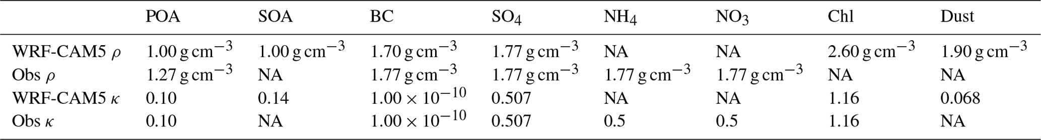
NA: not available.
Vertical turbulence was approximated using vertical wind measurements from a high-resolution anemometer (Morales and Nenes, 2010). This calculation fitted a Gaussian curve to the updraft spectrum integrated over 1024 samples at 20 Hz. The characteristic turbulent updraft velocity (m s−1), proportional to the root of turbulent kinetic energy (TKE), was taken as 0.79*σ, where σ is the standard deviation of that Gaussian curve. The factor of 0.79 also comes from the derivation in Morales and Nenes (2010). This quantity is also output directly from WRF-CAM5, where it is used with the grid-scale updraft speed to construct a Gaussian updraft spectrum that is then used to calculate activation. Both characteristic updrafts are selected in the vertical range of 100–700 m that contained most flat BL flight legs.
Inversion height in observations is calculated using two methods. First, the LASIC ARM value-added product included inversion heights and strengths derived by the Heffter method based on potential temperature gradients (Pesenson, 2003). At ASI, this produced between three and five height values in each radiosonde dataset. We selected the primary capping inversion height as the one with the largest corresponding inversion strength. The inversion top in WRF-CAM5 was calculated as the local maxima of θes (effective potential temperature of a saturated parcel) below ∼ 5 km and within 1 km above the first layer with RH >85 % to denote the boundary layer as well as the inversion base. We also applied the same algorithm to the raw radiosonde profiles as applied to WRF-CAM5 to account for algorithm performance differences. The ARM data also included similar estimates of PBL depth from the algorithm of Liu and Liang (2010) but did not report inversion strength, so they are not used here. In all the methods, inversion strength was calculated at each respective inversion height as a difference in potential temperature θ between the inversion base and top.
Two rain gauges were used for LASIC to help account for orographic lifting potentially impacting rain rates at the ARM station (Zuidema et al., 2018b). The ARM station was situated in the more mountainous and elevated eastern half of the island (7.967∘ S, 14.350∘ W). The UK Met Office rain gauge was located at the UK air base and meteorology station approximately 6 km to the west in a relatively flat region of the island (7.967∘ S, 14.4∘ W). Thus, the differences between them are to be expected and are not driven by instrument uncertainty.
2.3 Instrument intercomparison and selection
To make useful comparisons between models and observations from different field campaigns, we must understand the variability between the instruments used in each campaign. To this end, Barrett et al. (2022) compared multiple cloud and aerosol instruments on ORACLES and CLARIFY aircraft as well as the LASIC ARM station and found broadly consistent measurements between similar instruments on each, focusing especially on the joint flight day (18 August 2017) on which both the ORACLES and CLARIFY aircraft flew close together through smoke and clouds near ASI. This comparison showed that there was good agreement for BC, aerosol number concentration, and aerosol size distributions. Chemical compositions from the SP2 and ToF-AMS in ORACLES and CLARIFY were also shown by Barrett et al. (2022) to be within instrument uncertainty and within 1 standard deviation for most species. The ORACLES AMS reported a 40 % higher sulfate mass that was not attributable to likely instrument uncertainty or postprocessing. The LASIC Aerosol Chemical Speciation Monitor (ACSM) also measured composition, but the resulting OA and SO4 measurements showed a tendency towards 2–4 times lower mass concentrations than either the ORACLES or CLARIFY AMS. Diagnosing the reason for this difference is beyond the scope of this work. For the sake of consistent comparison between instruments without confounding uncertainty, we will focus on the two aircraft-mounted AMS instruments that have been shown to perform similarly.
Additionally, we performed a volume closure assessment between the ORACLES mass (AMS) and aerosol size (U. Hawaii UHSAS and PCASP) instruments for measurements in the free troposphere. WRF-CAM5 prescribes aerosol density per species as shown in Table 2, and we assumed values as shown for AMS-measured species. We found well-correlated volume closure with low error between the UHSAS, PCASP, and AMS (Fig. A1). This suggests first that the PCASP, with its higher upper size range around 3 µm, was not capturing aerosols that would have been missed with the UHSAS upper size cutoff of 1 µm. Second, both correlated well with the AMS total volume given the density assumptions below. This tells us that there was no significant aerosol mass beyond what the AMS was able to capture, such as dust and sea salt. This is also evident in the UHSAS size distributions (see Sect. 3.1.1).
Chloride mass concentration is not used from the ORACLES AMS data as it provided unrealistically high values in the middle and upper FT. This is consistent with the processing of the public data from the LASIC ACSM and CLARIFY AMS, which have similar issues measuring chloride in biomass smoke. As mentioned above, a volume closure suggests that there is very little chloride by mass in the FT, so we expect little impact on FT smoke properties.
The CLARIFY CCN are not analyzed for this work, as our primary usage of CCN data is to calculate hygroscopicity. PCASP, as the available instrument resolving size distributions in the CLARIFY dataset, has both a lower size resolution and a larger lower-end size cutoff (∼100 nm) than the UHSAS that both lead to large uncertainty in deriving κ.
2.4 WRF-CAM5 configuration
This work uses the WRF-Chem model, version 3.4 (Skamarock et al., 2008). We utilize the CAM5 aerosol and physics parameterizations (Chen et al., 2015; Ma et al., 2014; Zhang et al., 2015), which include the Modal Aerosol Module (MAM3) aerosol representation with three lognormal size modes (Liu et al., 2012), Fountoukis and Nenes (2005) series cloud droplet activation, Morrison and Gettelman (2008) two-moment cloud microphysics, ice nucleation via Niemand et al. (2012), and the Bretherton–Park (University of Washington) boundary layer turbulence scheme (Bretherton and Park, 2009). Note that the Fountoukis and Nenes (2005) activation scheme differs from the standard CAM5. The aerosol scheme is coupled with gas-phase and aerosol-phase chemistry of the Carbon Bond Mechanism version Z (CBMZ) (Zaveri and Peters, 1999). Natural dust emissions come from the DustDEAD emission algorithm (Zender et al., 2003). This configuration of WRF-CAM5 is used because it resembles the configuration used in global climate models, improvement of which is an extended goal of this research. We also use this model because it contains chemistry, aerosol–cloud feedbacks, and aerosol–radiation feedbacks, which are highly relevant for absorbing smoke and aerosol–cloud interactions. The model was configured with a horizontal grid resolution of 36 km with 72 vertical layers at 5 hPa spacing and a domain covering the southern burning region of Africa and the SEA. The National Centers for Environment Prediction-Final (NCEP-FNL) climatology (National Centers for Environmental Prediction, National Weather Service, NOAA, U.S. Department of Commerce, 2000) is used to initialize meteorology and boundary conditions. The anthropogenic emissions and trace gases for this study come from EDGAR-HTAP (Janssens-Maenhout et al., 2012), while fire emissions come from QFED2 (Darmenov and da Silva, 2015). QFED2 is provided at daily time resolution and 0.1∘ spatial resolution. A superimposed diurnal cycle is applied to resemble real burning trends such as that applied to an NCAR WRF-Chem build in Ye et al. (2021).
As described in previous work (Diamond et al., 2022), there is no subgrid shallow cumulus scheme enabled, as we discovered that it led to significant suppression of the boundary layer height and clouds compared to observations. Also, we do not use any subgrid scheme for smoke plume injection, and emissions are placed within the first model level. This is done as fires in the region tend to be small and the boundary layers over land are deep, so few injections above the boundary layer are expected. This assumption produces reasonable smoke layer heights over the southeastern Atlantic (Shinozuka et al., 2020). MAM3 uses three predefined lognormal size modes with fixed width and mean diameter at emission, after which the mass and number evolve freely but the width is kept fixed. We also changed emissions to exclude the “other PM2.5” category (i.e., total PM2.5 − OC − BC) in the emission files. Before our change, this was then added to the accumulation-mode aerosol mass in the dust category. With “other PM2.5” classed as dust, the modeled dust concentration in the lower FT was ∼ 8 µg m−3 across ORACLES samples and ∼ 5.5 µg m−3 across CLARIFY samples, or about 30 % and 35 %, respectively, of the total accumulation-mode mass in those samples. We consider this dust mass to be an unrealistically large mass when comparing it to observations of low-dust conditions in the FT during ORACLES and CLARIFY. Cloud droplets are activated in the model based on both aerosols at the cloud base and further secondary aerosol activation within the cloud.
Following suggestions in recent work (Diamond et al., 2022; Shinozuka et al., 2020) comparing multiple models to ORACLES data as well as our own calculations in the FT, we adjusted aerosol size parameters of the accumulation mode – applied across all species – to bring the model closer in line with observations. In particular, the geometric mean diameter (i.e., count mean diameter) of the accumulation-mode emissions was changed from 110 to 150 nm, and its standard deviation was changed from 1.8 to 1.5. These changes are consistent with both ORACLES observations and estimates in the literature of crop-burning primary emission sizes (Hays et al., 2005; Li et al., 2007; Winijkul et al., 2015; Zhang et al., 2011). The refractive index of organic carbon is set at 1.45+0i, and that of black carbon is 1.85+0.71i for optical property calculations.
The model run period starts on 15 July 2017 and is run through 31 August 2017. The July portion is discarded as meteorology and emission spinup time, but it allows smoke to circulate through the SEA region. Initial aerosol and chemical concentrations come from CAMS (Inness et al., 2019). For the entire run period, the model is re-initialized every 5 d and runs for 7 d at a time, with the first 2 d used to spin up the meteorology. The aerosol conditions are carried over from day 5 of the previous 7 d run cycle, and the meteorology is re-initialized to NCEP-FNL. This allows aerosols to evolve continuously, while meteorology remains relatively close to reanalysis. This setup also allows several days for aerosol–climate feedbacks to manifest, such as smoke heating in the FT, which may substantially alter subsidence and transport (Adebiyi and Zuidema, 2016).
We also uncovered a bug in the diagnostic CCN number calculations within the mixing and activation scheme: the model was not calculating a dynamic mean aerosol diameter based on total mass and number per mode but instead was using a prescribed value from the MAM aerosol-mode definitions. This led to an overestimation of all CCN concentrations in the output, although cloud activation was unaffected as CCN is recalculated separately based on the dynamic particle diameter. This bug was reported to the WRF-Chem development team, who have now released a fix. However, any WRF-Chem build up to v4.2.1 or model source code obtained before 15 January 2021 may be affected. This bug may have substantially impacted studies using WRF-Chem that reported on CCN concentrations directly, a not uncommon practice when reporting on aerosol–cloud interactions. Note that further usage of the terms “WRF” or “WRF-CAM5” in this work refers exclusively to the configuration described here.
2.5 Analytical methods
In the FT, our goal was to select smoky periods during relatively level flight legs. We focus on periods of uniform smoke behavior in the FT in particular to eliminate background aerosol signals and reduce in-sample variability. We therefore selected 8 min segments from 1 min merged data that contiguously met the threshold criteria for altitude and smokiness. This 8 min time interval represents roughly 55–100 km of aircraft travel, which in a straight line would pass through two model grid cells on average and was chosen to smoothen the observational variability. In ORACLES, we selected data for aircraft height >1200 m, RH <80 %, and CO concentration >120 ppb. We also limited samples to those segments with average total aerosol mass concentrations >5 µg m−3 and BC >100 ng m−3. This is similar to the Shinozuka et al. (2020) threshold of BC >100 ng m−3 to identify smoke plumes, and we incorporate AMS data availability as a key requirement for our analysis. In CLARIFY, we selected for the same height and RH, CO >100 ppb, total aerosol mass >1 µg m−3, and BC >50 ng m−3 to account for further plume dispersion over long distances. In both campaigns we selected flight legs with minimal altitude changes (less than 100 m over the sample period) to avoid sampling vertically stratified distinct smoke layers. We then extracted comparable observations and co-located model quantities for each variable of interest.
We treat the MBL as generally well-mixed for the purposes of smoke comparison. Boundary layer segments were selected in ORACLES by a threshold of altitude Z<1000 m, RH <95 %, and BC concentration >100 ng m−3. Boundary layer segments were selected in CLARIFY by z<1200 m, RH <95 %, and CO >100 ppb. These thresholds were used to maximize data availability and consistency and avoid sampling within clouds. The higher-altitude threshold in CLARIFY is to allow more data samples with the typically deeper and decoupled boundary layer near ASI, and the usage of a CO threshold rather than BC for smokiness in CLARIFY is a compromise considering data availability from the SP2.
A different modeling system was used to estimate smoke age, using the WRF Aerosol Aware Microphysics (WRF-AAM) configuration that was used regularly and reliably to forecast smoke transport throughout the ORACLES campaign (Redemann et al., 2021), and as such, we expect it to provide a reasonable estimate of the observed smoke age. To estimate smoke age, biomass-burning tracers tracking each day of emissions over the whole African continent were added to WRF-AAM. The concentration of the tracer from each day was used to calculate a weighted average of the emission day at a given point in space and time, thus giving an estimate for the average age of that plume. The age extracted from WRF-AAM is used as an age estimate for WRF-CAM5 and the observations. Given the differences in transport between all three of WRF-AAM, WRF-CAM5, and reality, the WRF-AAM age estimation method does not provide a perfectly Lagrangian age estimate following the plume itself. However, it still gives insight into bulk property changes in the smoke over time.
Clouds are analyzed by comparing the vertical profile of droplet number concentration (CDNC or NC) to below-cloud aerosol concentration. Cloud droplet data points are based on averaging 1 s resolution CDP data as the P3 and Bae146 FAAM aircraft profiled a cloud layer. These passes occurred over a relatively short horizontal distance (approximately 3 km) relative to the size of stratocumulus cloud decks, and thus they are treated as vertical cloud profiles. When sawtooth routes were flown (diving up and down through a cloud layer multiple times in close succession), the profile mean values from each single cloud profile were then averaged together. The selection of cloud profiles from the ORACLES datasets followed the same criteria as Gupta et al. (2021), and CLARIFY cloud selection used similar methods. Following the methods of Diamond et al. (2018), we report droplet-mass-weighted NC recorded by the same probe. This deemphasizes regions of extremely thin clouds and emphasizes regions with high liquid water.
For WRF, we calculate below-cloud aerosol by averaging across the two grid cells immediately below the cloud base, which were defined by a weighted droplet concentration threshold of 0.1 cm−3. For observations, the below-cloud aerosol was calculated as an average over the roughly 100 m sampled below the cloud base. To account for differences in vertical placement of clouds and MBL heights in the model vs. observations, all model cells below 3 km with weighted NC above the 0.1 cm−3 threshold were considered regardless of vertical structure. The model grid cells were co-located using the average latitude and longitude of the transect.
Here we present the findings of our model–observation comparison, commenting on both direct performance and indications of missing or inadequate smoke- and cloud-related processes in the model. We first analyze the free troposphere and then the boundary layer. These regions are meaningfully distinct in many ways. For example, the free troposphere has very low background aerosol generation, minimal precipitation during this study, and strong winds driving advection with limited vertical mixing. Thus, smoke is primarily driven from the continent in the free troposphere before entraining into the MBL. In the boundary layer, on the other hand, smoke is subject to strong turbulent mixing, cloud processing and deposition, and the ocean as a very strong source of sea spray aerosols and sulfate precursor gases. Aerosol behavior in both regions is important for constraining overall smoke and cloud evolution, but aerosols in the FT and MBL must each be considered in their own contexts.
3.1 Free troposphere
The free troposphere is where biomass-burning smoke in the SEA advects the furthest and with the least disturbance from clouds and other aerosol formation processes. We evaluate it first, both to understand WRF-CAM5 performance in representing BBA as it exists and evolves on its own and as a prerequisite for interpreting aerosol properties and processes when the smoke has mixed with background aerosols and clouds. This section will first analyze representation of total smoke amount and size, moving on to composition and then hygroscopicity. Finally, we evaluate evidence of significant chemical aging in smoke on timescales of several days, especially through losses of OA.
3.1.1 Smoke concentrations and size distributions
The FT is the logical starting point to evaluate model representation of biomass-burning smoke aerosols. In August and September, the smoke from the continent travels throughout most of the SEA region in the FT, with occasional entrainment into the boundary layer (Diamond et al., 2018). As a result, the lower FT (cloud top up to roughly 3 km) has a much higher and more consistent concentration of smoke than the boundary layer. Additionally, the boundary layer is itself a source of new aerosol particles that confound the smoke signal – primarily sulfates, salts, and organic particles from sea spray (Meskhidze et al., 2013; Zorn et al., 2008). The capping inversion frequently keeps this aerosol population from mixing heavily into the FT, and so it can constitute a large fraction of the BL aerosol mass even under smoky conditions.
Our analytical framework here supports and expands earlier conclusions about WRF-CAM5 performance. We find that the model FT accumulation-mode mean number concentration is biased high by 28 % compared to ORACLES observations (Fig. 2a) and by 38 % compared to CLARIFY (Fig. 2b). The WRF-CAM5 volume concentration is comparable to ORACLES (Fig. 2c, WRF-CAM5 mean bias % vs. UHSAS and −16 % vs. PCASP) and relatively high compared to CLARIFY (Fig. 2d, WRF-CAM5 mean bias % vs. PCASP). The total aerosol mass concentration simulated by WRF-CAM5 has mean biases of −10 % compared to ORACLES and +108 % compared to CLARIFY (Fig. 2e–f), tracking the trend in volume. These larger relative discrepancies with CLARIFY may be explained by a lack of mass loss through aging in WRF-CAM5 or insufficient scavenging, which will be discussed later. WRF-CAM5 underestimates CO in the FT by 31 % compared to ORACLES and 32 % compared to CLARIFY (Fig. 2g–h).
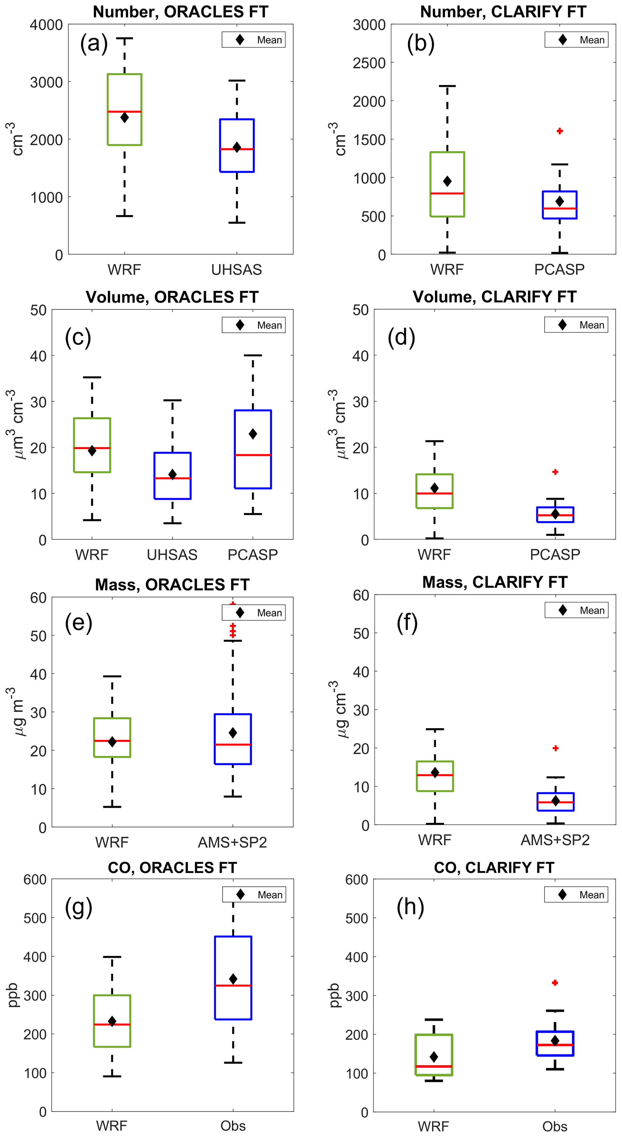
Figure 2Extensive properties of smoke in the free troposphere (FT) comparing WRF-CAM5 and appropriate instruments from both ORACLES and CLARIFY in 2017. Red line represents the sample median, black diamond represents the mean, and the small red crosses are outliers (greater than 1.5 times the interquartile range beyond the box). (a–b) Number concentration; (c–d) volume concentration; (e–f) mass concentration compared to combined AMS and SP2 mass measurements; (g–h) CO concentration.
WRF-CAM5 represents the range of geometric mean diameters well and is closest to the U. Hawaii UHSAS (Fig. 3a). The 25th–75th percentiles of samples of the geometric mean diameter are as follows: WRF, 186–208 nm; UHSAS, 176–196 nm; PCASP, 220–244 nm; LDMA, 208–231 nm. The model lognormal distribution also closely follows the spread and mean of observations on a representative sampling day (24 August 2017) despite a bias towards a high model number (Fig. 3b–c). The variability between instruments is not unexpected, and we conclude that, after observationally constraining smoke aerosol size at the point of emission, WRF-CAM5 can successfully represent the mean particle diameters after transport to the SEA to within instrument uncertainty.
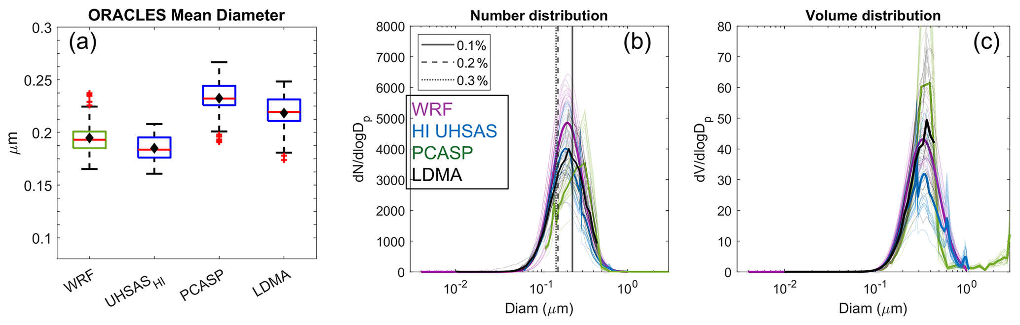
Figure 3Size properties in the free troposphere from both the WRF-CAM5 and ORACLES instruments. CLARIFY data are excluded here for lack of available instruments with a comparable size range. (a) Geometric mean diameter across all FT samples deemed smoky and flat enough. Figure features are defined in the caption for Fig. 2. (b–c) Number and volume size distributions of the same instruments from 31 August 2017, showing both the WRF-CAM5 nucleation and accumulation modes. The mean distribution from each data source is represented with a thicker line, with each underlying distribution as a thinner curve. Superimposed on panel (b) are the calculated Dcrit based on the CCN and GIT UHSAS in the three primary supersaturation settings.
Two other important features are visible in the number and volume distributions of free-tropospheric smoke from ORACLES. In the number size distributions (Fig. 3b), there is a dominant accumulation mode (50–440 nm in WRF-CAM5) and an extremely small number concentration of coarse-mode (>1 µm) or Aitken-mode (<40 nm) particles. This holds across >90 % of smoky ORACLES samples in the FT on other days (not shown). The lack of a coarse mode is supported by the volume size distribution from PCASP (Fig. 3c, green), showing that in the great majority (∼95 %) of our ORACLES cases there is no substantial volume of coarse particles such as mineral dust or sea spray. The volume closure between the AMS, PCASP, and UHSAS supports this. The smoke sampled here is days old, and any new particle formation that would generate an Aitken mode was likely in the past near the source in Africa. The LDMA, with its lower size range of around 10 nm, supports this notion.
3.1.2 Chemical composition and hygroscopicity
The average composition fractions across the FT samples in ORACLES and CLARIFY are shown in Fig. 4. The mass fraction of OA, by far the dominant chemical species, is captured well in the FT across the campaigns (Fig. 4b–c, h–i). Mass fractions of BC and SO4 are also comparable in the FT. As noted above, AMS analysis does not include chloride salts or mineral dust, but these are likely a very small component of FT aerosols regardless. WRF-CAM5 also lacks aerosol nitrate and ammonia in its implementation of MAM3. WRF-CAM5 also treats aerosol modes as internally mixed, similar to calculations based on the AMS.
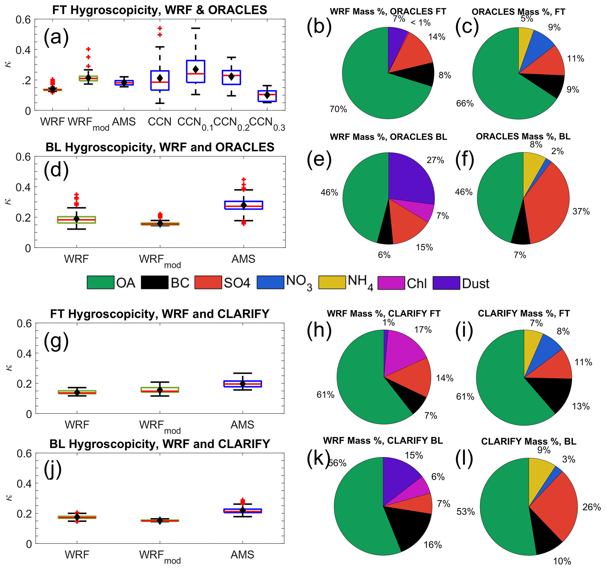
Figure 4Hygroscopicity and the corresponding properties of smoke in the FT and BL between the model and observations. (a) Hygroscopicity from WRF-CAM5 (green), first with all species and then excluding dust and chloride to match AMS (“mod” subscript), AMS-based, and data from the Nenes group, grouped and then disambiguated by CCN supersaturation setting. Calculations were made with the CCN and GIT UHSAS together. (d, g, f) Hygroscopicity from WRF-CAM5 and AMS for each campaign and atmosphere level. (b, c, e, f, h, i, k, l) Average composition by the mass fraction of smoke in ORACLES and CLARIFY FT and BL and co-located WRF-CAM5 samples. Model OA here includes secondary OA, a distinct model variable. WRF-CAM5 SOA was generally less than 3 % of the total mass.
The single-parameter hygroscopicity factor κ is biased low in the FT against AMS (−0.042 bias in ORACLES, −0.059 bias in CLARIFY) and against CCN (−0.046 bias in ORACLES) (Fig. 4a, g). When excluding dust and chloride to match the AMS, model bias tends to improve against observations in the FT (medians +0.075 in ORACLES and +0.011 in CLARIFY). The CCN and UHSAS from ORACLES had irregular availability and discontinuous supersaturation percentage (SS%) sampling in the BL compared to the FT and are unable to be separated by SS%, as done in the FT. Thus, MBL κ calculations based on CCN are not included in this comparison.
We suggest a few potential explanations for the low model κ bias. First, in our configuration, WRF-CAM5 lacks nitrate or ammonia aerosols, both of which increase the bulk hygroscopicity since and are both roughly assumed to be 0.5. Second, WRF-CAM5 retains around 10 % of the total aerosol mass as dust, which in the model has a very low hygroscopicity of 0.068. This dust comes from the natural dust emission scheme and is not related to fire emissions. Third, the prescribed properties for OA in the model may not be physically accurate. WRF-CAM5 uses a prescribed κOA of 0.1 and a density of 1.0 g cm−3. The set density of 1.0 g cm−3 for OA in WRF-CAM5 is low compared to both lab studies (Kuwata et al., 2011) and campaign-wide assumptions used in other studies, such as 1.27 g cm−3 (Wu et al., 2020). An erroneously low model density leads to a larger volume, which decreases κ since it is a volume-weighted mass average. An OA density of 1.27 g m−3 also produces the best volume agreement between the ORACLES AMS, UHSAS, and PCASP. The existing literature measuring the density of BBA organics over long aging periods is generally limited, but there is evidence that OA density is increased by at least 30 % – and up to 90 % – over the course of a few days (Dinar et al., 2006; Kuwata et al., 2011). KOA may realistically have values ranging from 0 to 0.2, with nonlinear dependence on age and oxidation level (Kacarab et al., 2020; Kuang et al., 2020; Wonaschütz et al., 2013; Duplissy et al., 2011).
WRF-CAM5 and AMS show a similarly narrow range in κ despite the bias in the mean. This indicates that the average bulk composition fractions of observed BBAs vary little as far as the AMS is capable of measuring. The hygroscopicity based on CCN shows a notably large spread, however. This is partially a result of convoluted instrument uncertainties (combining CCN and UHSAS instrument variability) and partially a result of the κ estimation strategy. The AMS measures bulk chemical mass, while the κ based on the UHSAS + CCN critical diameter (Dcrit) depends on the properties of the aerosol population around that size. At 0.1 % CCN SS, Dcrit fell in the range of 100–250 nm near the middle of the accumulation mode in most cases. At 0.2 % and 0.3 %, Dcrit was in the range of 60–180 nm, with Dcrit at 0.3 % ∼10 nm lower on average than at 0.2 %. Values of κ tend to be higher at 0.1 % SS (mean κ=0.27) than at 0.2 % (mean κ=0.22) and at 0.3 % (mean κ=0.10). As larger particles were less likely to contain refractory black carbon (rBC) or a lower rBC mass fraction in ORACLES (Sedlacek et al., 2022; Dobracki et al., 2023). This may reflect a composition dominated by more hydrophilic species such as sulfuric acid. This variability overall supports existing findings that the accumulation mode is at least partially externally mixed, especially at lower sizes (Denjean et al., 2020; Taylor et al., 2020; Sedlacek et al., 2022; Dahlkötter et al., 2014; Dobracki et al., 2023), which results in measurable differences in hygroscopicity. Imagery of ORACLES and CLARIFY particles also suggests that large BB particles very often mix with hygroscopic salts (Dang et al., 2022). This will be supported further by examining hygroscopicity using LASIC data in Sect. 3.2.3. The internal mixing assumption in WRF-CAM5 renders it unable to capture these observed features.
3.1.3 Aging processes
Biomass-burning aerosols emitted in southern Africa take roughly 4–14 d to be advected to the remote marine FT, leading to optically thick smoke layers reaching as far west as ASI and beyond (Chand et al., 2009; Zuidema et al., 2016). Over time, particles may undergo drastic physical and chemical changes such as heterogeneous oxidation, fragmentation, coagulation, and photolysis – impacting mass, density, optical properties, or hygroscopicity (Dinar et al., 2006; Dang et al., 2022; Dobracki et al., 2023; Che et al., 2021). There is consistent observational evidence of a loss of organics with increasing smoke age and oxidation markers in ORACLES and CLARIFY observations (Che et al., 2022; Dang et al., 2022; Sedlacek et al., 2022; Dobracki et al., 2023). Lab studies have suggested that, on the ∼ 3–14 d timescales relevant to these observations, this loss may be caused by heterogeneous oxidation – especially fragmentation – that functions to re-volatilize and evaporate organics (Kroll et al., 2009; O'Brien and Kroll, 2019; Che et al., 2021). This configuration of WRF-CAM5 forms SOA by predefined conversion factors applied to various organic gases such as isoprene and xylene. The density and hygroscopicity of each separate aerosol chemical species involved are constant.
The aerosol size distribution also evolves through new particle formation, coagulation, and evaporation. Here, we analyze the evidence of some aging processes in ORACLES observations and their representation, or lack thereof, in WRF-CAM5.
Mean particle diameter is a useful indicator of both particle evolution and CCN activity (Kuang et al., 2020). The mean diameter calculated using the ORACLES and CLARIFY PCASP instruments shows a nonmonotonic change with age, with a general trend towards growth over the 4–6 d range and then a flattening or decreasing diameter thereafter (Fig. 5a). The PCASP is used here because it was the only available sizing instrument across both the ORACLES and CLARIFY campaigns and therefore illuminates longer-term trends than ORACLES alone. The trend of mean diameter growth in the first ∼ 3–7 d is also captured by the ORACLES LDMA and UHSAS (Fig. A2). However, as ORACLES has very few samples aged beyond ∼ 7 d, the flattening or decreasing diameter trend cannot be corroborated by the more highly size-resolved instruments here. WRF-CAM5 shows an overall positive trend (Fig. 5c) – the mean diameter grows steadily from approximately 185 to 230 nm between 4 and 12 d. This is expected as the model lacks a mechanism to lose OA particle mass over time, while particles can grow through coagulation and secondary aerosol condensation. There is no evidence of wet scavenging in the FT – either in the model or the observations – that might otherwise allow new particle formation to assert itself in a previously smoky FT air parcel.
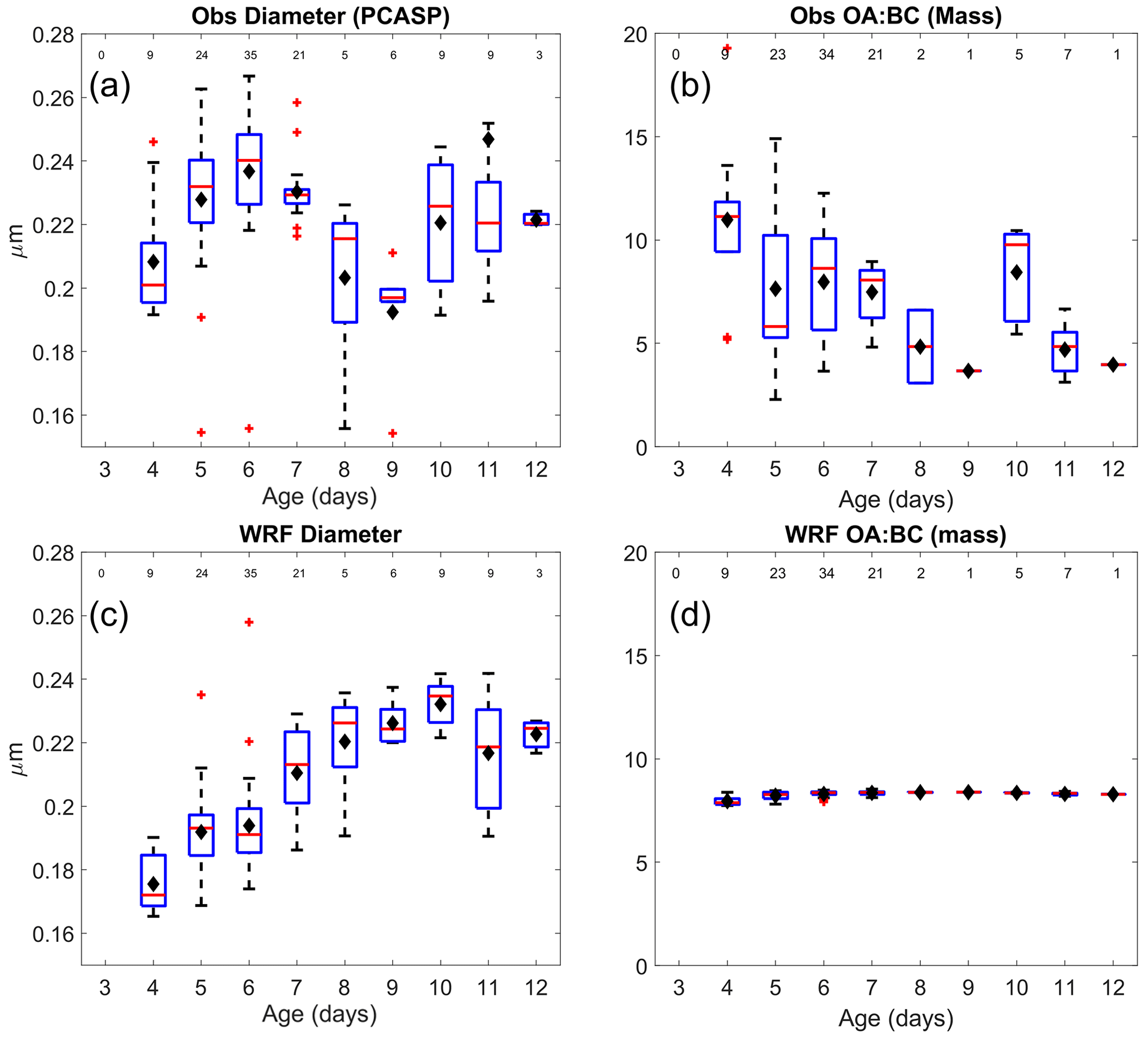
Figure 5Aging trends in FT for mean diameter (a, c) and OA:BC mass ratio (b, d). Sample sizes for each box–whisker plot are listed at the top of each figure. Observational data are filtered for total aerosol mass >10 µg m−3 and rBC mass >0.1 µg m−3, and the same subset is then sampled in WRF-CAM5. Black diamonds represent the mean, and red lines represent the median.
Additionally, observations show a noisy downward trend in the OA:BC mass ratio over time (Fig. 5b), while in the model the ratio is nearly completely flat (Fig. 5d), which implies negligible SOA formation in the model. Further, the mass ratio of OA:CO decreases by 54 % between the ORACLES and CLARIFY FT samples but only decreases by 30 % in WRF-CAM5 (not shown). This decrease is to be expected as the smoke dilutes and approaches the background CO concentration in the region, roughly ∼ 60 ppb measured during the clean periods at ASI in August 2017 (Pennypacker et al., 2020). In contrast, BC : CO decreases very similarly in both observations and the model (14 % and 17 % decreases, respectively). Taken together, OA is likely selectively lost over time in a way that the model does not represent. Quantification of this loss rate and these specific causal mechanisms, such as fragmentation or photolysis, has been explored in other field, modeling, and lab studies (Lou et al., 2020; Che et al., 2021; Sedlacek et al., 2022; O'Brien and Kroll, 2019; Konovalov et al., 2019; Dobracki et al., 2023) and could be implemented and tested in the SEA and compared to these observations to assess improvements and impacts.
3.2 Marine boundary layer
The MBL in the SEA region presents new observational and modeling challenges that are not present in the FT. The MBL represents a new source of primary and secondary aerosols in the form of sea spray and dimethyl sulfide (DMS) emissions. Smoke is entrained into the MBL at sporadic spatial and temporal scales and is removed by precipitation in similarly irregular ways that complicate 1:1 comparison (Diamond et al., 2018). The MBL has convective turbulence that leads to stratocumulus formation at the capping inversion, and the MBL close to ASI can transition to being frequently thermodynamically decoupled between the surface layer and cloudy layer (Zhang and Zuidema, 2019). All these processes can have strong impacts on the composition and size distribution of aerosols and change how they may interact with clouds.
This section focuses primarily on the LASIC campaign. First, it is worth noting some substantial differences between LASIC observations and the airborne ones used so far (ORACLES and CLARIFY). The LASIC campaign's static nature on ASI means its observations are subject to the whims of meteorology and cannot seek out smoke parcels as aircraft can. Smoke also only reaches ASI when it has been entrained – either locally or upwind – into the BL.
Second, as ASI is approximately 3000 km west of Angola, smoke is substantially more aged and diluted in both CLARIFY and LASIC data than the smoke measured during ORACLES. For the purposes of this work, LASIC analysis will be limited to August 2017 since that is when it overlapped with both ORACLES and CLARIFY. It is also worth noting that, at 36 km resolution, WRF-CAM5 treated the cells containing ASI as ocean uniformly, and so the model includes no meteorological features related to land or topography.
Figure 6a–e show the time series of smoke properties and rain at ground level at ASI. We have identified and labeled periods considered smoky, medium, and clean for the sake of separating smoke properties during this month by regime, based on tercile concentrations of black carbon similar to Zhang and Zuidema (2019). This section compares WRF-CAM5-modeled properties to observations of the BL aerosol properties, size distribution, hygroscopicity, and mixing state and concludes with an analysis of boundary layer dynamics and rain in observations and WRF-CAM5 ASI through the month.
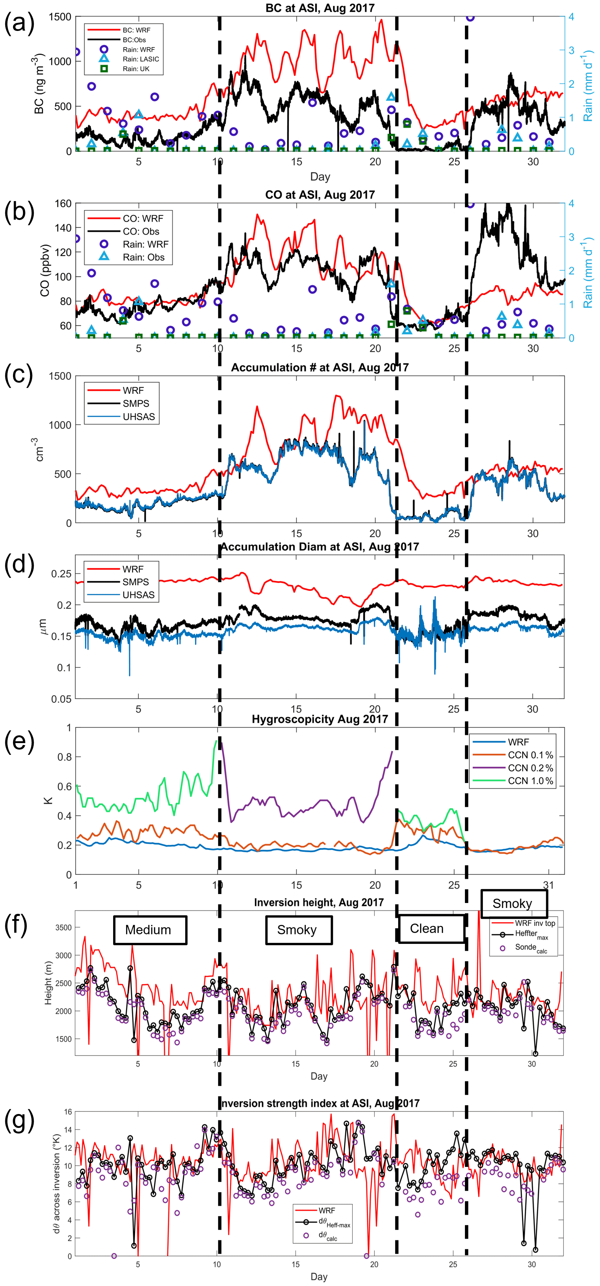
Figure 6Time series of smoke properties at ASI in August 2017. Vertical dashed lines delineate periods of smoky, medium, and clean conditions. (a–b) Refractory BC and CO concentrations, respectively. Overlaid on both are rainfall accumulation from WRF-CAM5, LASIC, and UK Met devices summed on each day. (c) Accumulation-mode number concentration. (d) Accumulation-mode geometric mean diameter. (e) Hygroscopicity from the CCN and SMPS from LASIC and bulk composition in the accumulation mode in WRF-CAM5. (f) PBL inversion height from WRF-CAM5, from the LASIC radiosonde VAP, and recalculated from radiosonde matching the algorithm applied to WRF-CAM5. (g) Inversion strength from WRF, from the LASIC radiosonde VAP, and recalculated from radiosonde profiles using the same algorithm as applied to WRF-CAM5.
We first analyze the physical properties of smoke measured in the BL, especially as its size distribution and hygroscopicity vary under different smoke loading conditions. We then discuss model trends in smoke entrainment and wet scavenging at ASI. Finally, we evaluate the aerosol–cloud activation tendencies in BL aircraft measurement and WRF-CAM5, together with the TKE captured in both.
3.2.1 Smoke concentrations and size distributions
While WRF-CAM5 shows reasonable representation of FT mean diameters of smoke aerosols, it broadly overestimates the mean diameter of smoke at ASI (WRF: ∼ 200–240 nm; LASIC: 150–190 nm; WRF-CAM5 mean biases of +35 % vs. SMPS and +47 % vs. UHSAS, Fig. 6d). This is likely due to a lack of particle losses from multiple sources. First, there are potential chemical losses in single particles (see Sect. 3.1.2). Second, there may be a shrinking mean diameter of the aerosol size distribution following aerosol activation into cloud droplets and wet scavenging, in which larger particles are activated and collected more easily. This process leads to a 10 % decrease in diameter near ASI at the end of August 2017 (Wu et al., 2020), and heavy precipitation has been observed in North American boreal forest to potentially be very efficient at removing large smoke particles (Taylor et al., 2014). These occur over long distances as particles in WRF-CAM5 continue to coagulate and grow.
The accumulation-mode number concentrations are overpredicted in WRF-CAM5 by 60 % on average (Fig. 6c), excluding the clean period, and by over 1000 % during the clean period. The bias is lowest during the smokiest period, with a median bias of 45 % and an interquartile range of 14 %–80 %. The overestimation bias is far larger during the clean period (over 1000 %). Some of the bias is attributable to the number concentration bias in the FT, as this smoke with high NAER entrains into the BL (WRF-CAM5 bias above ORACLES and CLARIFY of ∼ 28 %–38 %), and the remainder may be explained by either over-entrainment or removal issues as discussed below.
The observed number size distribution shows a consistent accumulation mode centered around 180 nm through both smoky and medium periods (Fig. 7a–c) that corresponds to the smoke transferred from the FT (Fig. 3b). During clean periods, observations show a dominant Aitken mode with a mean diameter of 30–50 nm (Fig. 7c), which remains comparable in number to the Aitken mode under medium loading conditions and is almost nonexistent during smoky periods. As the smoky FT showed nearly no Aitken mode, the BL particles below ∼ 40 nm are likely coming from new particle formation driven by marine or smoke SO2 precursors under clean conditions (Zheng et al., 2021). We hypothesize that the observed Aitken-mode particles observed under clean conditions are gradually lost through either coagulation with the accumulation-mode smoke after it entrains or through cloud processing that combines the Aitken and accumulation modes. This could explain why the Aitken mode is present for clean and medium-level smoke but is not observed for smoky conditions. In WRF-CAM5, the Aitken mode tends to be very small in number and broader than observations. This could be due to new particle formation in the model being suppressed by the constant presence of smoke but could also be due to the potential inability of models to properly represent new particle formation under pristine marine conditions, as found by previous work (Tang et al., 2022).
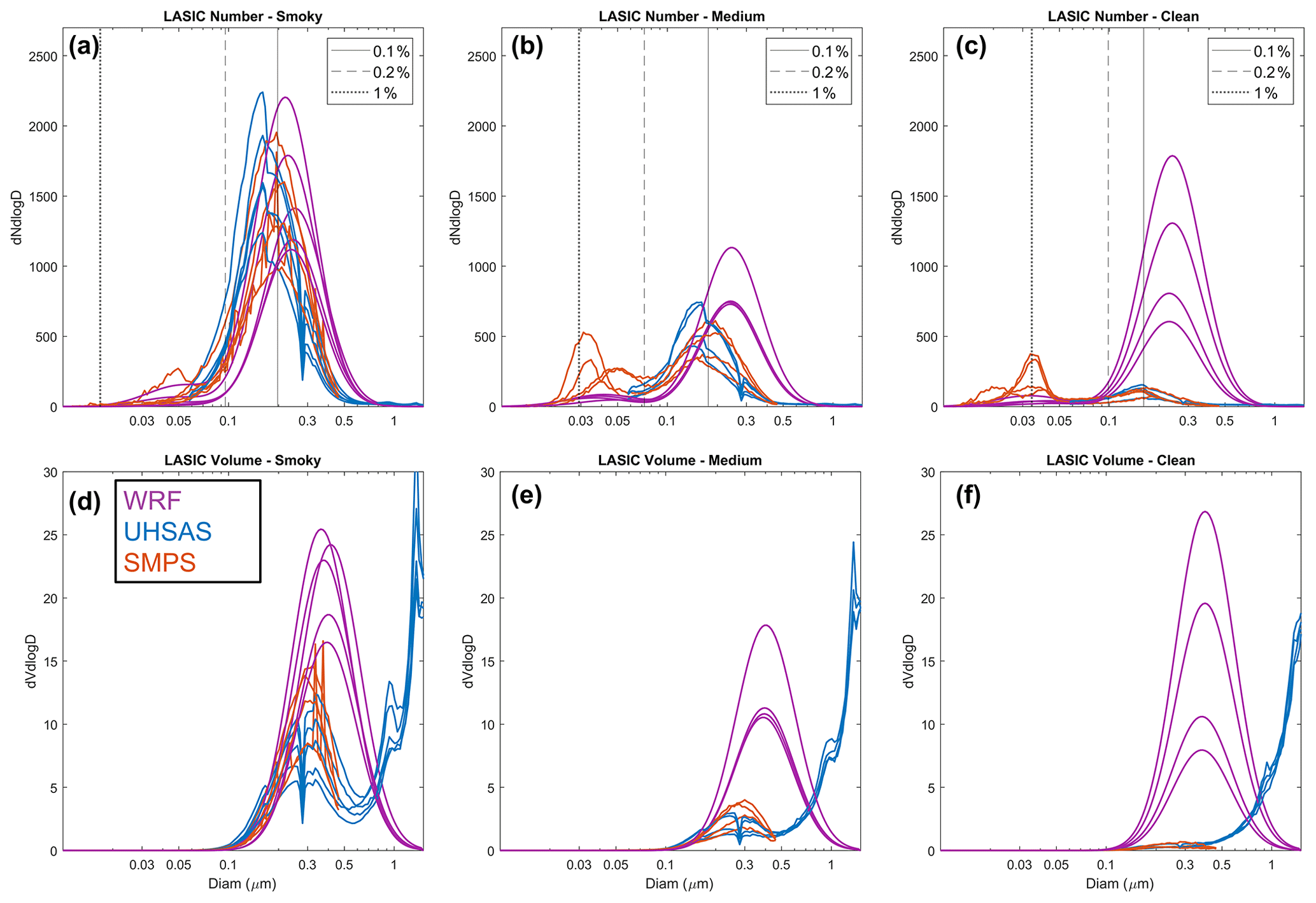
Figure 7Number and volume distributions from LASIC selected to be representative of the range of conditions under smoky, medium, and clean conditions at ASI. WRF-CAM5 plots show the sum of the accumulation- and nucleation-mode lognormals.
There is also a persistent population of coarse aerosols through this period that predominantly impacts volume. The UHSAS volume distributions at ASI show a large coarse mode above 1 µm regardless of smokiness (Fig. 7d–f). This coarse mode also does not appear in most ORACLES FT data (Fig. 3b–c), suggesting that its emergence at ASI is not driven by smoke. The likely source is sea spray in the MBL (Dedrick et al., 2022; Saliba et al., 2019; Clarke et al., 1998). A caveat in this dataset is that the LASIC ARM emplacement was within ∼ 500 m of a sea cliff, where winds and breaking waves may represent a large, localized particle source that is much less influential elsewhere in the SEA BL.
3.2.2 Chemical composition and hygroscopicity
Observations from both the ORACLES and CLARIFY AMSs show a large difference in particle composition between the FT and the boundary layer (e.g., Fig. 4c vs. 4f) that is generally not captured in WRF-CAM5. Although the OA mass fraction is still comparable in the OA between the model and the observations, the BC and especially SO4 fractions are inconsistent. In particular, WRF-CAM5 does not reproduce the large increase in sulfate fraction in the BL compared to the FT. By mass fraction, sulfate in observations is enhanced from 11 % to 26 % in the CLARIFY FT to BL and from 11 % to 37 % in the ORACLES FT to BL. Since free tropospheric smoke is chemically similar between the observations and the model, this discrepancy in the BL is unlikely to be related to a model misrepresentation of smoke aerosol composition itself. It could instead be a combination of WRF-CAM5 having weaker sulfate aerosol formation in the MBL – with this WRF-Chem build not including DMS emissions – as well as a lack of OA removal. SO2 is also co-emitted with smoke and tends to only weakly condense into sulfate aerosol in the FT, but aqueous chemistry drives more efficient condensation in the BL (Fiedler et al., 2011; Bianco et al., 2020; Rickly et al., 2022). Therefore, there may be a low model bias in either source emissions of SO2 or in their aqueous chemical processing that limits model representation of the FT-to-MBL SO4 gradient. There is also observational evidence of regular and frequent occurrences of new particle formation in the upper part of the remote MBL (Zheng et al., 2021; Abel et al., 2020) that have been hypothesized as being driven by DMS and thus containing sulfate. These could then subside into the BL and may be a locally dominant source of sulfate and new particles (Clarke et al., 1998). WRF-CAM5 also retains a large dust fraction in the ORACLES-sampling BL that does not appear in the observations as described above. This suggests a model bias towards high fine-mode dust generation rates in the natural dust emission scheme, which is an issue previously identified in dust parameterizations (Kok, 2011).
Estimates of κ based on chemical composition rely on total volume, so the accumulation mode and the coarse mode are the dominant populations impacting chemical κ. Compared to BL observations from the ORACLES and CLARIFY AMS, WRF-CAM5 κ remains biased low against the AMS (−0.089 bias in ORACLES, −0.084 bias in CLARIFY) (Fig. 4d, j). If chloride and dust are excluded to mimic the AMS, the model bias grows (to median biases of −0.117 in ORACLES and −0.105 in CLARIFY). The higher sulfate fraction in the BL compared to the FT drives the corresponding higher BL κ, as seen by comparing the FT and BL composition in each sample set (e.g., Fig. 4b vs. 4e and 4c vs. 4f).
However, the number distribution is most relevant to CCN-based κ because it is used to determine Dcrit at a given SS. Under all conditions, the Dcrit at 0.1 % SS generally falls in the middle of the accumulation mode around 170–200 nm (Fig. 7a–c), and thus we expect that mode to be more representative of bulk smoke κ. Dcrit at 0.2 % SS falls in the range of 75–95 nm, which is in the lower tail of the accumulation mode for smoky periods and tends to be in the overlap region of the nucleation and accumulation modes for clean and medium-smoke periods. Dcrit at 1.0 % SS is centered in the Aitken mode (15–35 nm). κ at 0.2 % SS has been excluded from Fig. 6e during clean and medium-smoke periods, and at 1.0 % SS it has been excluded from Fig. 6e during smoky periods, as the very low number concentration around their respective Dcrit in these periods leads to highly unreliable κ estimates and eclipses meaningful analysis.
Focusing on the smoky period, LASIC κ at 0.2 % CCN supersaturation is larger by a factor of 2 than at 0.1 % SS (κ ∼0.2 at 0.1 % SS vs. κ ∼0.45 at 0.2 % SS). Based on these estimates of κ, the most hygroscopic particles are those near the lower tail of the accumulation mode. Therefore, during smoky periods it may be supposed that these are predominantly sulfate, nitrate, or ammonium particles or a combination of coagulation and condensation of the same onto the less hygroscopic BBAs. This is broadly in line with the hygroscopicity of Aitken-mode particles during clean and medium-smoke periods, with a similar range of κ. However, this contrasts with the FT κ values discussed in Sect. 3.1.2, where κ in the 40–150 nm range is ∼0.13, which is lower than κ in the bulk of the accumulation mode. This suggests that processes in the MBL impact the hygroscopicity of the lower tail of the accumulation mode, even in periods of high-smoke loading.
WRF-CAM5 closely approximates the CCN-based κ from LASIC at 0.1 % SS and diverges greatly at 0.2 % SS (Fig. 6e). The narrow model variability in κ is explained by the consistent smoky conditions in WRF-CAM5 at ASI through this period, echoing the comparison to ORACLES. WRF-CAM5 also considers particles to be totally internally mixed within each mode, negating the possibility of compositional differences at different size ranges within one mode. With limited chemical evolution and no size-based differentiation possible in each mode, it is reasonable that the model does not produce large hygroscopicity changes. A deeper analysis of observed coating thicknesses and size-resolved particle compositions is beyond the scope of this work.
3.2.3 Smoke entrainment, removal, and rain at Ascension Island
The period of extremely low BC concentration (<50 ng m−3) observed by the LASIC SP2 between 20 and 25 August is generally not matched by WRF-CAM5. The model shows median BC concentration biases of +1080 % (+280 ng m−3) during the same period when shifting by 1 d to account for the time lag vs. observations and +1950 % (+310 ng m−3) when matched to observed times directly. However, during medium and smoky periods the BC timing is captured well, matching the September 2016 findings of Shinozuka et al. (2020). WRF-CAM5 showed median BC biases of +66 % (+330 ng m−3) during the smoky periods and +190 % (250 ng m−3) during the medium period. This contrasts with the FT, where WRF-CAM5 does not show a strong bias in smoke BC by either mass (Shinozuka et al., 2020) or mass fraction (Fig. 4b, h). Therefore, the high model bias in the BC amount at ASI suggests that the model overestimates smoke entrainment, underestimates smoke removal in the boundary layer, or both. We analyze evidence of both possibilities here.
CO is broadly considered a passive smoke tracer on timescales of weeks that is not removed by wet or dry scavenging of aerosols (Avey et al., 2007; Freitas et al., 2005; Garrett et al., 2010). After a smoke plume is processed by clouds and the aerosols are largely removed by coalescence and precipitation, the CO co-emitted with BBAs is expected to remain as a tracer of smoke presence. Thus, CO is a good tracer to isolate smoke entrainment. Figure 6a–b show a time series of both BC and CO at ASI overlaid with rain measurements. We find that BC remains significantly higher in WRF-CAM5 than observations through most of August, while for CO the model tracks observations more closely. This points towards the model likely having unrealistically weak aerosol removal in the BL. If the main issue were overestimation of smoke entrainment, then CO would show similar overprediction to BC during the clean period because they entrain together.
Another piece of evidence supporting weak modeled aerosol removal on the BL can be seen by comparing the first (10–21 August) and second (26–31 August) smoky periods (Fig. 6a, b). Observed BC and CO enhancements in these periods are significantly different (e.g., CO in period 2 is larger than in period 1, while BC is slightly less), while the model shows closer BC and CO enhancements for both periods. Subtracting a conservative estimate of 50 ppb background CO concentration, the first and second smoky periods have observed median BC:ΔCO ratios of 0.0092 and 0.0064 (units µg m−3 : ppbv), respectively. A higher assumed background CO of 60 ppb – as seen in a fire-off run of WRF-CAM5 over this same period (Fig. A3) – would only amplify this discrepancy. The model has BC:ΔCO ratios of 0.0146 and 0.0160 for the first and second periods, respectively. With no consideration of background concentration, the first and second periods showed BC:CO ratios of 0.0049 and 0.0037 in observations and 0.0085 and 0.0067 in WRF-CAM5, respectively. A likely explanation for the observed behavior is the different degrees of BL aerosol removal in the air masses reaching ASI in these two periods. A lack of this strong aerosol removal can explain the low degree of BC:CO variability in the model. These two pieces of evidence, together with the model overprediction of mean diameters in the BL (Sect. 3.2.1), make a compelling case for concluding that aerosol removal in the BL is likely too weak compared to reality. Notably, the observed clean period from 21 to 25 August is likely caused by advection of clean air parcels to the island rather than removal, as evidenced by the very low CO concentration for the season (Pennypacker et al., 2020).
To better understand potential wet aerosol removal, we evaluate the model's ability to represent precipitation (Fig. 6a). We find that rain is far more frequent overall in the model than in the two observational datasets. The distribution of 3-hourly rain accumulation in the model, on the other hand, skews towards lower rainfall volume in each period than in the observations, even when limiting the model rain samples to only include those above the LASIC rain bucket detection threshold of 0.05 mm h−1 (Fig. 8). This is consistent with the well-known “drizzling problem” of global climate models (Chen et al., 2021; Stephens et al., 2010; Trenberth et al., 2003; Trenberth and Zhang, 2018). The underprediction of heavy rain events could be one of the reasons explaining weak aerosol removal if they are more efficient than light drizzle at removing aerosols, although future work is needed to implement parameterizations that may tackle this issue (e.g., Chiu et al., 2021) and evaluate it in the context of aerosol removal.
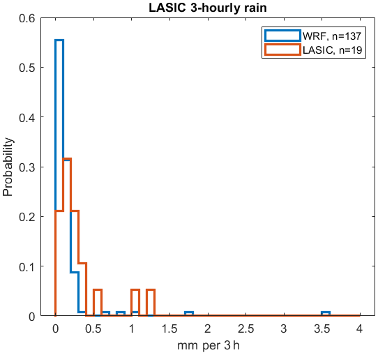
Figure 8Histogram of the 3-hourly rain rate measured by LASIC. In the legend, “n” represents the total number of rain events sampled over the detection threshold of 0.05 mm h−1. Note that UK Met rain data are only archived daily and are not included here.
Entrainment can be modulated by boundary layer height (BLH) and inversion strength (Wilcox, 2010; Karlsson et al., 2010), and thus these are included in this evaluation (Fig. 6f–g). WRF-CAM5 shows reasonably good correlation with LASIC radiosonde observations of these two metrics. The model BL is slightly higher than observations, with median biases of +220 m (+10 %) during this month compared to the Heffter BLH and +400 m (+21 %) compared to the recalculated BLH values based on the model algorithm. When only analyzing the clean and medium-smoke loading periods, the bias is higher at +330 m or +15 % median bias compared to Heffter, and it is +510 m or +27 % compared to the recalculation. A deeper BL can result in enhanced smoke entrainment as smoke does not have to subside as much to reach the BL top, increasing the availability of smoke to entrain. On the other hand, WRF-CAM5 inversion strength is well-represented or slightly overestimated depending on the calculation used, with median biases of +0.14 K (+1.1 %) compared to Heffter and +1.7 K (+21 %) compared to the recalculation. A stronger inversion would be expected to lead to less mixing across this boundary and thus less entrainment, opposing potential effects due to a deeper BL (Wilcox, 2010; Karlsson et al., 2010). Thus, given that BLH and inversion strength biases are low and might result in opposite behavior, these do not support a persistent overprediction of entrainment. This is consistent with the time series of CO (Fig. 6b), which show a range of behaviors from CO overprediction (e.g., first smoky period) to underprediction (e.g., second smoky period), implying a mixed behavior of model entrainment and not necessarily a persistent bias.
3.2.4 Aerosol activation and turbulence
ORACLES and CLARIFY took measurements of aerosols and cloud properties at fine scales, in close proximity to both, and with strong controls on the sampling location. This avoids some of the assumptions and screening algorithms that add uncertainty to assessments based on remote-sensing measurements and provides better vertical resolution and sampling within clouds.
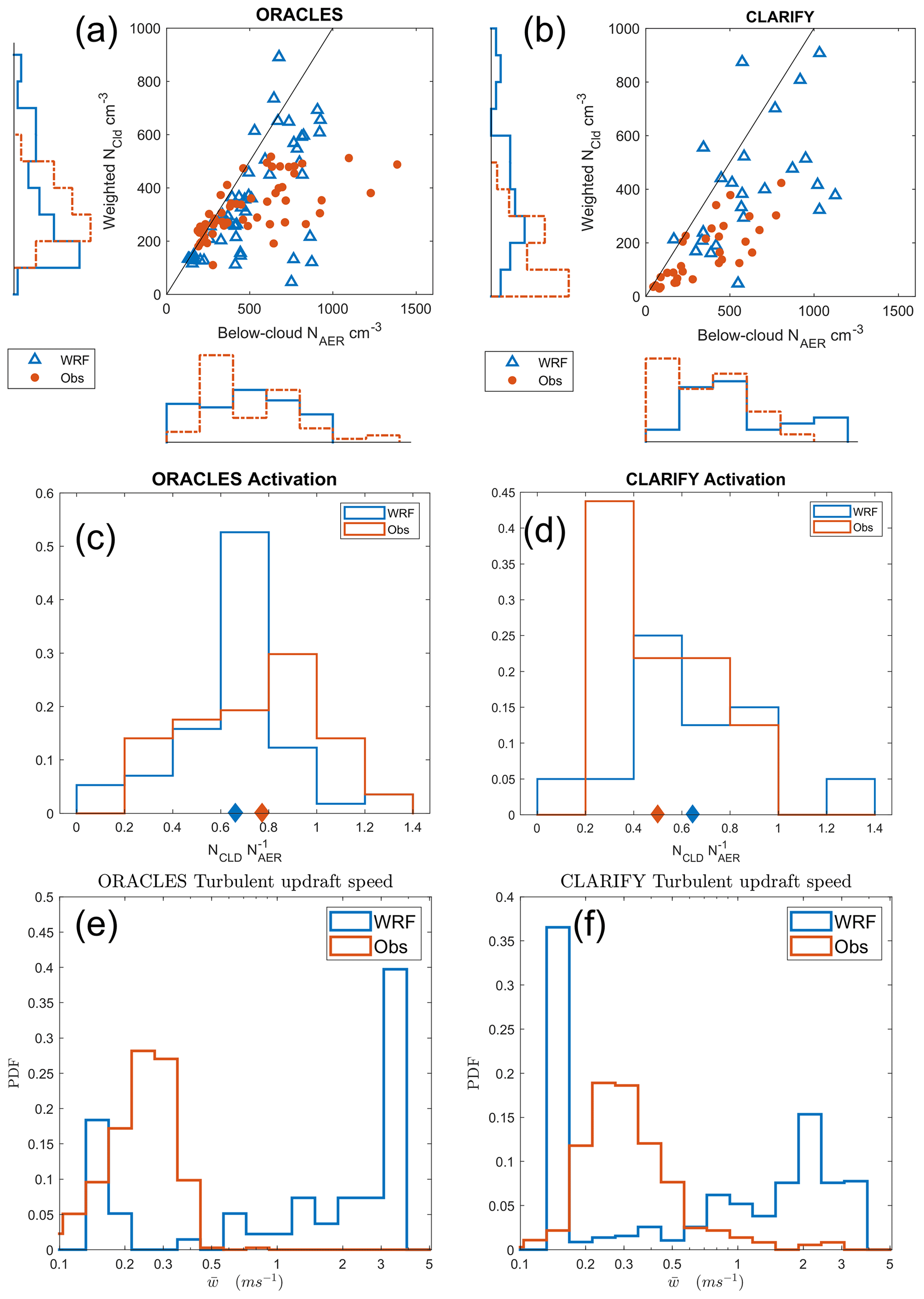
Figure 9Observed and modeled cloud properties and BL turbulence. (a–b) Cloud droplet number (weighted by LWC – liquid water concentration) compared against below-cloud aerosol concentration from observations and WRF-CAM5 in (a) ORACLES and (b) CLARIFY cloud transects. Axes of panels (a) and (b) show the kernel probability distribution functions (PDFs) of each distribution on the same scale. (c–d) Normalized PDFs of activation efficiency and the ratio for each campaign and WRF-CAM5. Diamonds on the x axes represent the median of the similarly colored population. (e–f) Spectra of BL turbulent updrafts from each campaign and WRF-CAM5 between 100 and 700 m. Note: the aerosol number concentration in observations is taken from PCASP for consistency across campaigns, which has a lower size limit of ∼110 nm. This cutoff was also virtually imposed on the WRF-CAM5 size distribution for this figure.
Aerosol activation into cloud droplets is analyzed here by comparing observed and modeled values of both mass-weighted cloud droplet number concentration (NC) and average aerosol number concentration (NA) immediately below that cloud, sampled across CLARIFY and ORACLES. A bias visible in WRF-CAM5 that does not appear in either ORACLES (Fig. 9a) or CLARIFY (Fig. 9b) observations is that the modeled clouds have a much higher upper limit of NC. Observations show an upper range of 400–500 cm−3 across both campaigns, while WRF-CAM5 attains nearly 1000 cm−3. This may be driven by strong updraft turbulence driving high activation as described below.
CLARIFY observations also capture a cloud population with both NC<150 cm−3 and NA<300 cm−3 that was not seen in ORACLES or WRF-CAM5. This difference between campaigns may be due to the more scattered clouds and more diluted smoke sampled in CLARIFY than in ORACLES. It may also represent a cloud population that is not substantially impacted by smoke, considering the low number concentration. As mentioned in the previous section, WRF-CAM5 has consistently high (>400 cm−3) smoke concentrations around ASI throughout August, so it fails to represent the low smoke cloud interactions observed there.
The ratio of NC to NA, representing a rough aerosol activation efficiency, is shown in Fig. 9c–d. The median activation efficiencies are 0.77 for ORACLES, 0.50 for CLARIFY, and 0.66 and 0.64 for the respective WRF-CAM5 samples. The shift in activation efficiency spectra between ORACLES and CLARIFY, together with the aerosol and cloud number concentration spectra, may reflect a change in the predominant cloud domain, such as that from stratocumulus to cellular cumulus, which is not captured well in the model (Abel et al., 2020; Diamond et al., 2022; Zuidema et al., 2018b).
Turbulent updraft strength is the main driver of the water vapor supersaturation within a lifted parcel and thus the activation tendency of an aerosol population (Ditas et al., 2012; Prabhakaran et al., 2020). Compared to both ORACLES and CLARIFY BL measurements, WRF-CAM5 substantially overestimates the updraft strength (Fig. 9e–f) and has a bimodal TKE distribution rather than the unimodal character of observations. The large peak in TKE distribution near 0.15 m s−1 in WRF-CAM5 comes from a coded lower limit on TKE. These strong updrafts could generate a population of erroneously high NC if conditions are suitable, which could explain why the model does not capture the observed NC upper limit. We also note that the spread of NC in the model is much larger than the observations (NC standard deviation in observations =101 cm−3; in WRF it is 219 cm−3), while this is not the case for NA (observed standard deviation =227 cm−3; in WRF it is 236 cm−3), which can also be explained by an overpredicted spread in model TKE. If the model is under-mixing ambient air into clouds, despite the high TKE, it will also be underestimating dilution of NC. Testing this would require further aircraft observations beyond the scope of this work. The observed probability distributions of TKE are consistent between the ORACLES and CLARIFY anemometers despite the large spatial separation and are consistent with values for ORACLES reported by Kacarab et al. (2020).
This work has analyzed the performance of WRF-CAM5 against the ORACLES, CLARIFY, and LASIC field campaigns. The goal has been to assess model representation of biomass-burning smoke and aerosol–cloud interactions in the SEA, especially focusing on diagnosing process differences. Previous work and our analyses show that different instruments on the same aircraft platform and across platforms are often sufficiently consistent to compare jointly with the model, expanding our analysis and conclusions.
In the FT, WRF-CAM5 captures the average physical and chemical properties of the younger smoke measured by ORACLES but shows larger and consistent positive biases for the older smoke measured by CLARIFY. This implies issues with model representation of smoke aging. The mean diameter is captured within variability in the ORACLES observations after increasing the initial diameter in model emissions to be more consistent with literature and observed values. Although smoke composition in the FT is represented well in the model, especially the fractions of OA, sulfate, and BC, we find that WRF-CAM5 underpredicts hygroscopicity by ∼ 25 %–35 % in the smoky FT. This κ bias could be caused by a lack of NH4 and NO3 in the model, overprediction of dust, and misrepresentation of OA properties (e.g., low prescribed density and κ as well as the change in those values with age).
Notably, in both the ORACLES and LASIC observations, we find that CCN-estimated κ exhibits a large range of smoky conditions across different particle sizes in the 20–300 nm range. FT (ORACLES) smoke shows a lower κ in the lower tail of the accumulation mode compared to the center (κ ∼0.1 vs. ∼0.3, respectively), likely due to a larger fraction of black carbon at lower sizes. This suggests a large variance in the mixing state across the accumulation mode that WRF-CAM5 is not able to capture, as it assumes total internal mixing per mode.
By comparing mean smoke properties using modeled age estimates in the FT, we find that WRF-CAM5 is likely missing significant aging processes impacting smoke mean diameter and composition. The OA:BC mass ratio and the OA:CO and BC : CO ratios compared across 4–12 d of transport show that OA is selectively being removed and therefore limiting particle growth, which is not represented by the model. This process is a valuable target for future work since the current literature studying smoke aging beyond several hours is limited and because simulated particle size can impact aerosol–cloud interactions and estimates of cloud radiative effects in the region.
Model evaluation in the boundary layer introduces processes such as DMS emissions, cloud processing, wet scavenging, and strong vertical mixing that strongly impact smoke evolution and properties and that have no consistent analog in the FT, leading to a new smoke evaluation regime. Our BL comparison focuses mostly on data from LASIC. First, we found that WRF-CAM5 is significantly overpredicting smoke amount (by mass and number) and diameter compared to LASIC. Some of this bias is likely tied to biases in the FT smoke that entrains, but a large part of the model discrepancy is likely due to scavenging differences. We also find that observations from LASIC show a substantial Aitken mode present under medium- and low-smoke conditions that is always lacking in the model. This is likely a combination of weak model scavenging and low model BL sulfate precursors contributing to weak new particle formation. Observations also show a consistent coarse mode throughout August that is not apparent in WRF-CAM5.
Observations of aerosol composition in the boundary layer show a 2.5–3 times relative enhancement of SO4 in the MBL compared to the FT in both ORACLES and CLARIFY, which is not represented by the model. This suggests that WRF-CAM5 has missing or weak processes that lead to sulfate aerosol in the MBL, such as BL ocean DMS emissions (not included in this model build), potentially insufficient BL SO2 from smoke, and smoke removal, all of which allow for periods of sulfate particle formation. During clean and medium-smoke loading periods, the LASIC SMPS also shows an Aitken mode that is likely driven by new particle formation and has hygroscopicity values similar to sulfate.
Hygroscopicity in MBL (LASIC) smoke, similar but opposite to the trend in the FT, varies between the lower tail of the accumulation mode and its center (κ∼0.5 vs. ∼0.2). This is likely caused by sulfate uptake of smaller particles through coagulation of the Aitken mode or precursor condensation. This suggests significantly different chemical compositions at different sizes and thus some external mixing within the accumulation mode. The fact that this trend is apparent at very different smoke ages and locations suggests that it is a consistent feature of smoke aerosols and one which WRF-CAM5 is not able to simulate due to its modes being internally mixed. This should be considered a mitigating factor in future studies of BBA hygroscopicity and composition, as both are highly size-dependent. A future sensitivity study using newer κ values for the AMS and the model – such as from Schmale et al. (2020), which is generally significantly higher than those used here – could provide further insight into the importance of κ and chemical composition in cloud activation.
The substantial overprediction of aerosol concentration in the MBL at ASI could be explained by either too-strong smoke entrainment or too-weak aerosol removal in the MBL, but multiple pieces of evidence point to the latter being the primary factor. First, mean aerosol diameter substantially decreases in observations from 180–240 nm in the CLARIFY and ORACLES FT to 140–180 nm in the LASIC MBL. The model shows little change in mean diameter. This points to cloud processing of aerosol rather than a smoke process on its own. Comparing the behavior of BL CO and BC concentrations can provide further insights. Also, observed BC : ΔCO ratios, assuming a background of 50 ppb CO, change substantially between the two heavily smoky periods ( in the first, 0.0064 in the second), which can be explained by differences in BC removal across the history of these air masses. This variation is weaker in the model ( in the first smoky period, 0.0160 in the second). We also find that WRF-CAM5 has rain that is far more frequent, though lighter, than observations support – in line with the known drizzle problem of global circulation models (GCMs) – which could contribute to a weak aerosol removal. Finally, model evaluations of inversion height, inversion strength, and MBL CO show modest biases (+10 %–21 %, +1.1 %, +0.5 % mean biases, respectively) that also oppose each other in illustrating entrainment tendency and overall do not support a persistent overestimation of entrainment. Under clean conditions, aerosols may have the largest relative impact on cloud droplet number (Kacarab et al., 2020) and are especially important to constraining aerosol–cloud radiative forcing (Gryspeerdt et al., 2023). An inaccurate representation of aerosol removal and smoke-free conditions should therefore be taken into account for future modeling analyses of aerosol–cloud–radiation interactions.
The activation ratio for below-cloud aerosols (0.1–3 µm) into liquid droplets is relatively constant in WRF-CAM5 samples in both ORACLES and CLARIFY at . However, observations show a higher activation tendency in ORACLES () and a lower activation tendency in CLARIFY (). The observed NC in both aircraft campaigns shows an upper limit of ∼ 400–500 cm−3, which is exceeded occasionally by WRF-CAM5 by 300–500 cm−3 across both campaigns and which leads to a wider modeled spectrum of NCLD. Vertical TKE was analyzed using both the ORACLES and CLARIFY anemometers. WRF-CAM5 is found to overestimate TKE by up to a factor of 10 in the boundary layer compared to both campaigns and shows a bimodal distribution rather than the observed unimodal distribution. The strong model turbulence may contribute to the model exceeding the upper limit of the observed NCLD and overpredicting the NCLD spread.
The performance of WRF-CAM5, despite its biases and missing processes, represents a useful tool for the study of smoke aerosols. LASIC, CLARIFY, and ORACLES present an especially rich suite of observations against which to compare model representations of major atmospheric processes such as boundary layer turbulence, smoke composition and size changes over long aging periods, and aerosol–cloud interactions (Shinozuka et al., 2020). Schemes allowing OA removal over aging timescales of ∼ 14 d may substantially improve composition and bulk optical properties in models and thus need to be tested in future work. Sulfate representation in the MBL may also be improved by improving DMS emission schemes, validating SO2 emissions and processing in smoke, and improving scavenging schemes that allow for ultra-clean regions to emerge and lead to significant new particle formation.
The impact of smoke evolution on cloud droplet nucleation is highly variable and remains difficult to model in GCMs, which commonly have simple aerosol evolution schemes and aerosol mixing-state assumptions as well as frequently coarse resolutions of ∼ 0.25–1∘. If TKE spectra can be improved, then a more accurate aerosol chemistry and mixing-state schema and better representation of aerosol removal in the MBL may improve cloud microphysical properties, which could help reduce uncertainties in modeled aerosol–cloud radiation interactions. Future work could use the similar methodology presented in this work to evaluate other modeling systems to assess whether similar biases are present and to implement model improvements. Finally, an assessment of how these improvements modify effective radiative forcings and climate impacts of smoke should be performed.
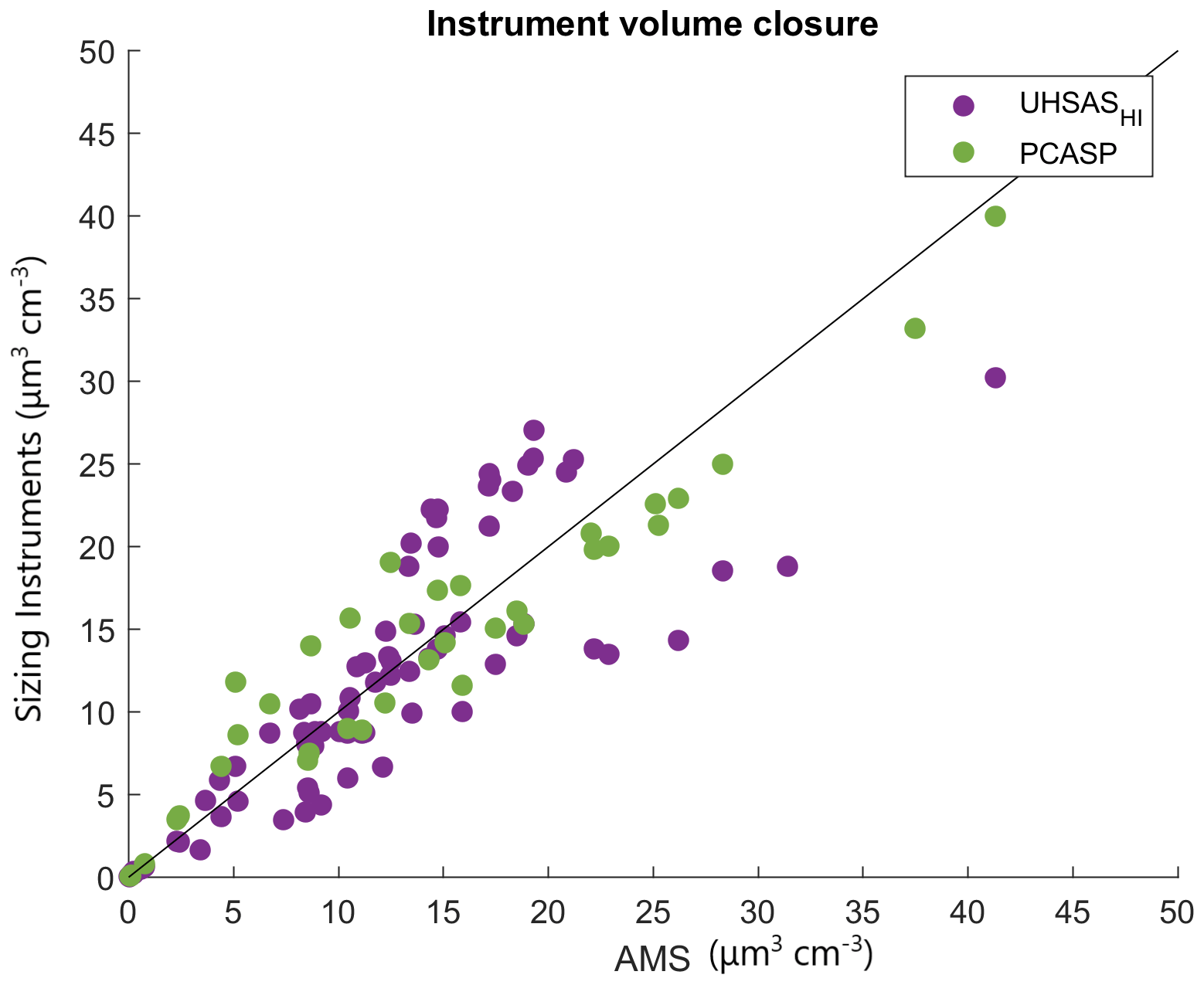
Figure A1Total volume concentration in the ORACLES FT, comparing both the U. Hawaii UHSAS and PCASP each against the AMS. Densities assumed for the AMS are listed in Table 2 of the main text.
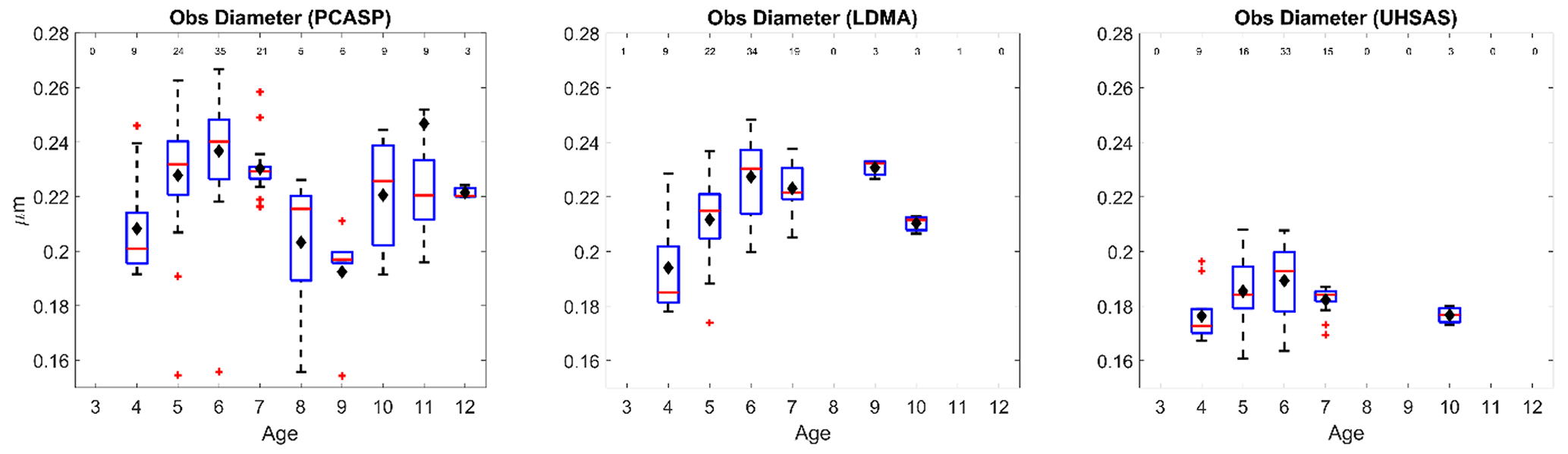
Figure A2Geometric mean diameter from observations, binned by WRF-AAM average plume age. The PCASP plot uses samples from both ORACLES and CLARIFY as it is the only aerosol sizing instrument available in both campaigns. LDMA and UHSAS are both only from ORACLES samples.
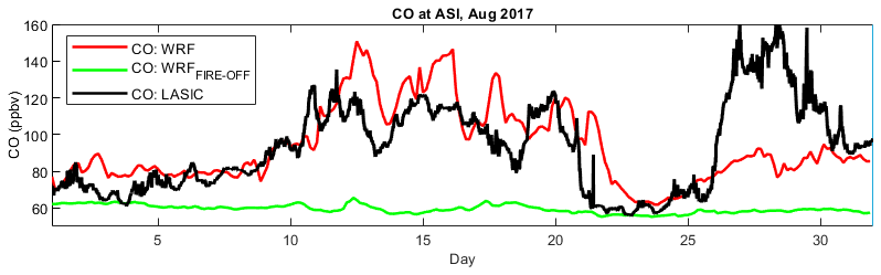
Figure A3CO concentrations from WRF-CAM5 both with and without QFED2 fire emissions to illustrate the model background and observations from LASIC for August 2017.
The VIIRS map is available in the NRT VIIRS 375 m Active Fire product VNP14IMGT distributed by NASA FIRMS and available online at https://earthdata.nasa.gov/firms (last access: 26 June 2022; NASA, 2022) and https://doi.org/10.5067/FIRMS/VIIRS/VNP14IMGT_NRT.002 (NASA, 2021).
Observational datasets for ORACLES 2017 and co-located WRF-AAM plume age estimates are available through the NASA ESPO data archive: https://espo.nasa.gov/ORACLES/archive/browse/oracles/id14/P3 (last access: 10 March 2020; ORACLES Science team, 2020).
Observational datasets for CLARIFY-2017 are available through the CEDA data archive: https://catalogue.ceda.ac.uk/uuid/38ab7089781a4560b067dd6c20af3769 (Facility for Airborne Atmospheric Measurements et al., 2017).
Datasets for LASIC are available individually as follows through the ARM data archive. Data were accessed between 1 August 2018 and 2 February 2022.
The weighing bucket precipitation gauge is available at https://doi.org/10.5439/1338194 (Atmospheric Radiation Measurement (ARM) user facility, 2017).
The Ultra-High-Sensitivity Aerosol Spectrometer is available at https://doi.org/10.5439/1333828 (Atmospheric Radiation Measurement (ARM) user facility, 2016a).
The Scanning Mobility Particle Sizer is available at https://doi.org/10.5439/1225453 (Atmospheric Radiation Measurement (ARM) user facility, 2016b).
The cloud condensation nuclei particle counter (column A) is available at https://doi.org/10.5439/1323892 (Atmospheric Radiation Measurement (ARM) user facility, 2016c).
The cloud condensation nuclei particle counter (column B) is available at https://doi.org/10.5439/1323893 (Atmospheric Radiation Measurement (ARM) user facility, 2016d).
The condensation particle counter (CPCF) is available at https://doi.org/10.5439/1352536 (Atmospheric Radiation Measurement (ARM) user facility, 2016e).
The radiosonde planetary boundary layer height is available at https://doi.org/10.5439/1150253 (Atmospheric Radiation Measurement (ARM) user facility, 2016f).
CH and PES designed the model–observation comparison. PES acquired the resources to support this research. AN, AD, SF, GMM, HC, JMH, SGH, CK, SG, MK, AN, JR, AJS, KLT, RW, JZ, JU, JP, and PZ provided data from instruments during the ORACLES, LASIC, and CLARIFY observation periods. CK, HW, JMH, JZ, PZ, SF, SG, SGH, and JU assisted with further analysis of observational data. CH led the model and observational data processing for this comparison with scripting assistance from PES. PES and CH ran the model and implemented configuration changes. CK, JPSW, JU, LRL, and YZ provided substantial components of the model configuration. CH wrote the first draft. PS provided major input throughout writing, and AJS, AND, GEM, JR, JZ, LRL, PZ, RW, SF, SG, SGH, and YZ provided further editing and feedback.
At least one of the (co-)authors is a guest member of the editorial board of Atmospheric Chemistry and Physics for the special issue “New observations and related modelling studies of the aerosol–cloud–climate system in the Southeast Atlantic and southern Africa regions (ACP/AMT inter-journal SI)”. The peer-review process was guided by an independent editor, and the authors also have no other competing interests to declare.
Publisher's note: Copernicus Publications remains neutral with regard to jurisdictional claims made in the text, published maps, institutional affiliations, or any other geographical representation in this paper. While Copernicus Publications makes every effort to include appropriate place names, the final responsibility lies with the authors.
This article is part of the special issue “New observations and related modelling studies of the aerosol–cloud–climate system in the Southeast Atlantic and southern Africa regions (ACP/AMT inter-journal SI)”. It is not associated with a conference.
ORACLES is a NASA Earth Venture Suborbital-2 investigation funded by the US National Aeronautics and Space Administration (NASA) Earth Sciences Division and managed through the Earth System Science Pathfinder Program Office.
We acknowledge the use of data and/or imagery from NASA's Fire Information for Resource Management System (FIRMS) (https://earthdata.nasa.gov/firms, last access: 26 June 2022), part of NASA's Earth Observing System Data and Information System (EOSDIS).
Financial support for this work was provided by NASA ORACLES grant no. 80NSSC19K1463 and funds from the Anthony and Jeanne Pritzker Family Foundation to Pablo E. Saide, DOE LASIC grant no. DE-SC0018272 to Paquita Zuidema and Pablo E. Saide, and the NERC CLARIFY-2017 Large Grant no. NE/L01358 to Jim M. Haywood and Hugh Coe. Jianhao Zhang was supported by DOE LASIC grant no. DE-SC0021250. Siddhant Gupta was supported by the NASA Earth and Space Science Fellowship (grant nos. NNX15AF93G and NNX16A018H). Greg M. McFarquhar and Siddhant Gupta were supported by NASA (grant no. 80NSSC18K0222). Yang Zhang is supported by the U.S. NOAA Office of Climate AC4 Program (grant no. NA20OAR4310293). L. Ruby Leung is supported by the Office of Science, U.S. Department of Energy Biological and Environmental Research, as part of the Regional and Global Model Analysis program area. Pacific Northwest National Laboratory is operated for the U.S. Department of Energy by Battelle Memorial Institute under contract no. DE-AC05-76RL01830. Athanasios Nenes acknowledges support from European Research Council project “pyroTRACH” (grant no. 726165).
This research has been supported by the U.S. Department of Energy (grant no. DE-SC0018272), the National Aeronautics and Space Administration (grant no. 80NSSC19K1463), UK Natural Research Environment Research Council Large (grant no. NE/L01358), U.S. Department of Energy DE-SC0021250, National Aeronautics and Space Administration Earth and Space Science Fellowship (grant nos. NNx15AF93G and NNx16A018H), National Aeronautics and Space Administration (grant no. 80NSSC18K0222), U.S. National Oceanic and Atmospheric Administration (grant no. NA20OAR4310293), U.S. Department of Energy, Pacific Northwest National Laboratory (grant no. DE-AC0576RL01830), and European Research Council project (grant no. 726165).
This paper was edited by Annele Virtanen and reviewed by three anonymous referees.
Abel, S. J., Barrett, P. A., Zuidema, P., Zhang, J., Christensen, M., Peers, F., Taylor, J. W., Crawford, I., Bower, K. N., and Flynn, M.: Open cells exhibit weaker entrainment of free-tropospheric biomass burning aerosol into the south-east Atlantic boundary layer, Atmos. Chem. Phys., 20, 4059–4084, https://doi.org/10.5194/acp-20-4059-2020, 2020.
Adebiyi, A. A. and Zuidema, P.: The role of the southern African easterly jet in modifying the southeast Atlantic aerosol and cloud environments, Q. J. Roy. Meteor. Soc., 142, 1574–1589, https://doi.org/10.1002/qj.2765, 2016.
Adebiyi, A. A. and Zuidema, P.: Low cloud cover sensitivity to biomass-burning aerosols and meteorology over the Southeast Atlantic, J. Climate, 31, 4329–4346, https://doi.org/10.1175/JCLI-D-17-0406.1, 2018.
Andela, N. and van der Werf, G. R.: Recent trends in African fires driven by cropland expansion and El Niño to La Niña transition, Nat. Clim. Change, 4, 791–795, https://doi.org/10.1038/nclimate2313, 2014.
Atmospheric Radiation Measurement (ARM) user facility: Ultra-High Sensitivity Aerosol Spectrometer (AOSUHSAS), 23 April 2016 to 1 November 2017, ARM Mobile Facility (ASI) Ascension Island, South Atlantic Ocean, AMF1 (M1), compiled by: Uin, J., Koontz, A., Salwen, C., and Hayes, C., ARM Data Center [data set], https://doi.org/10.5439/1333828, 2016a.
Atmospheric Radiation Measurement (ARM) user facility: Scanning mobility particle sizer (AOSSMPS), 20 May 2016 to 20 October 2017, ARM Mobile Facility (ASI) Ascension Island, South Atlantic Ocean; AMF1 (M1), compiled by: Kuang, C., Singh, A., Salwen, C., and Hayes, C., ARM Data Center [data set], https://doi.org/10.5439/1225453, 2016b.
Atmospheric Radiation Measurement (ARM) user facility: Cloud Condensation Nuclei Particle Counter (AOSCCN2COLA), 24 April 2016 to 31 October 2017, ARM Mobile Facility (ASI) Ascension Island, South Atlantic Ocean; AMF1 (M1), compiled by: Koontz, A., Uin, J., Andrews, E., Enekwizu, O., Hayes, C., and Salwen, C., ARM Data Center [data set], https://doi.org/10.5439/1323892, 2016c.
Atmospheric Radiation Measurement (ARM) user facility: Cloud Condensation Nuclei Particle Counter (AOSCCN2COLB), 24 April 2016 to 31 October 2017, ARM Mobile Facility (ASI) Ascension Island, South Atlantic Ocean; AMF1 (M1), compiled by: Koontz, A., Uin, J., Andrews, E., Enekwizu, O., Hayes, C., and Salwen, C., ARM Data Center [data set], https://doi.org/10.5439/1323893, 2016d.
Atmospheric Radiation Measurement (ARM) user facility: Condensation Particle Counter (AOSCPCF), 20 May 2016 to 31 October 2017, ARM Mobile Facility (ASI) Ascension Island, South Atlantic Ocean; AMF1 (M1), compiled by: Kuang, C., Singh, A., Cromwell, E., Andrews, E., Hayes, C., and Salwen, C., ARM Data Center [data set], https://doi.org/10.5439/1336393, 2016e.
Atmospheric Radiation Measurement (ARM) user facility: Planetary Boundary Layer Height (PBLHTSONDE1MCFARL), 29 April 2016 to 31 October 2017, ARM Mobile Facility (ASI) Airport Site, Ascension Island, South Atlantic Ocean; Supplemental Site (S1), compiled by: Riihimaki, L., Riihimaki, L., Zhang, D., and Zhang, D., ARM Data Center [data set], https://doi.org/10.5439/1991783, 2016f.
Atmospheric Radiation Measurement (ARM) user facility: Weighing Bucket Precipitation Gauge (WBPLUVIO2), 1 June 2017 to 1 November 2017, ARM Mobile Facility (ASI) Ascension Island, South Atlantic Ocean; AMF1 (M1), compiled by: Wang, D., Jane, M., Cromwell, E., Sturm, M., Irving, K., Delamere, J., and Mockaitis, M., ARM Data Center [data set], https://doi.org/10.5439/1338194, 2017.
Avey, L., Garrett, T. J., and Stohl, A.: Evaluation of the aerosol indirect effect using satellite, tracer transport model, and aircraft data from the International Consortium for Atmospheric Research on Transport and Transformation, J. Geophys. Res.-Atmos., 112, D10S33, https://doi.org/10.1029/2006JD007581, 2007.
Barrett, P. A., Abel, S. J., Coe, H., Crawford, I., Dobracki, A., Haywood, J., Howell, S., Jones, A., Langridge, J., McFarquhar, G. M., Nott, G. J., Price, H., Redemann, J., Shinozuka, Y., Szpek, K., Taylor, J. W., Wood, R., Wu, H., Zuidema, P., Bauguitte, S., Bennett, R., Bower, K., Chen, H., Cochrane, S., Cotterell, M., Davies, N., Delene, D., Flynn, C., Freedman, A., Freitag, S., Gupta, S., Noone, D., Onasch, T. B., Podolske, J., Poellot, M. R., Schmidt, S., Springston, S., Sedlacek III, A. J., Trembath, J., Vance, A., Zawadowicz, M. A., and Zhang, J.: Intercomparison of airborne and surface-based measurements during the CLARIFY, ORACLES and LASIC field experiments, Atmos. Meas. Tech., 15, 6329–6371, https://doi.org/10.5194/amt-15-6329-2022, 2022.
Bellouin, N., Quaas, J., Gryspeerdt, E., Kinne, S., Stier, P., Watson-Parris, D., Boucher, O., Carslaw, K. S., Christensen, M., Daniau, A. L., Dufresne, J. L., Feingold, G., Fiedler, S., Forster, P., Gettelman, A., Haywood, J. M., Lohmann, U., Malavelle, F., Mauritsen, T., McCoy, D. T., Myhre, G., Mülmenstädt, J., Neubauer, D., Possner, A., Rugenstein, M., Sato, Y., Schulz, M., Schwartz, S. E., Sourdeval, O., Storelvmo, T., Toll, V., Winker, D., and Stevens, B.: Bounding Global Aerosol Radiative Forcing of Climate Change, Rev. Geophys., e2019RG000660, https://doi.org/10.1029/2019RG000660, 2020.
Bianco, A., Passananti, M., Brigante, M., and Mailhot, G.: Photochemistry of the Cloud Aqueous Phase: A Review, Molecules, 25, 423, https://doi.org/10.3390/molecules25020423, 2020.
Bond, T. C., Doherty, S. J., Fahey, D. W., Forster, P. M., Berntsen, T., Deangelo, B. J., Flanner, M. G., Ghan, S., Kärcher, B., Koch, D., Kinne, S., Kondo, Y., Quinn, P. K., Sarofim, M. C., Schultz, M. G., Schulz, M., Venkataraman, C., Zhang, H., Zhang, S., Bellouin, N., Guttikunda, S. K., Hopke, P. K., Jacobson, M. Z., Kaiser, J. W., Klimont, Z., Lohmann, U., Schwarz, J. P., Shindell, D., Storelvmo, T., Warren, S. G., and Zender, C. S.: Bounding the role of black carbon in the climate system: A scientific assessment, J. Geophys. Res.-Atmos., 118, 5380–5552, https://doi.org/10.1002/JGRD.50171, 2013.
Boucher Dodman, D., Hayward, B., Pelling, M., Castan Broto, V., Chow, W., Chu, E., Dawson, R., Khirfan, L., McPhearson, T., Prakash, A., Zheng, Y., and Ziervogel, G.: Cities, Settlements and Key Infrastructure. In: Climate Change 2022: Impacts, Adaptation, and Vulnerability. Contribution of Working Group II to the Sixth Assessment Report of the Intergovernmental Panel on Climate Change, edited by: Pörtner, H.-O., Roberts, D. C., Tignor, M., Poloczanska, E. S., Mintenbeck, K., Alegría, A., Craig, M., Langsdorf, S., Löschke, S., Möller, V., Okem, A., and Rama, B., Cambridge University Press, Cambridge, UK and New York, NY, USA, 907–1040, https://doi.org/10.1017/9781009325844.008, 2022.
Bretherton, C. S. and Park, S.: A new moist turbulence parameterization in the community atmosphere model, J. Climate, 22, 3422–3448, https://doi.org/10.1175/2008JCLI2556.1, 2009.
Chand, D., Wood, R., Anderson, T. L., Satheesh, S. K., and Charlson, R. J.: Satellite-derived direct radiative effect of aerosols dependent on cloud cover, Nat. Geosci., 2, 181–184, https://doi.org/10.1038/ngeo437, 2009.
Che, H., Stier, P., Gordon, H., Watson-Parris, D., and Deaconu, L.: Cloud adjustments dominate the overall negative aerosol radiative effects of biomass burning aerosols in UKESM1 climate model simulations over the south-eastern Atlantic, Atmos. Chem. Phys., 21, 17–33, https://doi.org/10.5194/acp-21-17-2021, 2021.
Che, H., Segal-Rozenhaimer, M., Zhang, L., Dang, C., Zuidema, P., Dobracki, A., Sedlacek, A. J., Coe, H., Wu, H., Taylor, J., Zhang, X., Redemann, J., and Haywood, J.: Cloud processing and weeklong ageing affect biomass burning aerosol properties over the south-eastern Atlantic, Communications Earth & Environment, 3, 1–9, https://doi.org/10.1038/s43247-022-00517-3, 2022.
Chen, D., Dai, A., and Hall, A.: The Convective-To-Total Precipitation Ratio and the “Drizzling” Bias in Climate Models, J. Geophys. Res.-Atmos., 126, e2020JD034198, https://doi.org/10.1029/2020JD034198, 2021.
Chen, Y., Zhang, Y., Fan, J., Leung, L. R., and Zhang, Q.: Application of an Online-Coupled Regional Climate Model, WRF-CAM5, over East Asia for Examination of Ice Nucleation Schemes: Part I. Comprehensive Model Evaluation and Trend Analysis for 2006 and 2011, Climate, 3, 627–667, https://doi.org/10.3390/cli3030627, 2015.
Chiu, J. C., Yang, C. K., van Leeuwen, P. J., Feingold, G., Wood, R., Blanchard, Y., Mei, F., and Wang, J.: Observational Constraints on Warm Cloud Microphysical Processes Using Machine Learning and Optimization Techniques, Geophys. Res. Lett., 48, e2020GL091236, https://doi.org/10.1029/2020GL091236, 2021.
Christensen, M. W., Jones, W. K., and Stier, P.: Aerosols enhance cloud lifetime and brightness along the stratus-to-cumulus transition, P. Natl. Acad. Sci. USA, 117, 17591–17598, https://doi.org/10.1073/pnas.1921231117, 2020.
Clarke, A. D., Varner, J. L., Eisele, F., Mauldin, R. L., Tanner, D., and Litchy, M.: Particle production in the remote marine atmosphere: Cloud outflow and subsidence during ACE 1, J. Geophys. Res.-Atmos., 103, 16397–16409, https://doi.org/10.1029/97JD02987, 1998.
Cochrane, S. P., Schmidt, K. S., Chen, H., Pilewskie, P., Kittelman, S., Redemann, J., LeBlanc, S., Pistone, K., Kacenelenbogen, M., Segal Rozenhaimer, M., Shinozuka, Y., Flynn, C., Platnick, S., Meyer, K., Ferrare, R., Burton, S., Hostetler, C., Howell, S., Freitag, S., Dobracki, A., and Doherty, S.: Above-cloud aerosol radiative effects based on ORACLES 2016 and ORACLES 2017 aircraft experiments, Atmos. Meas. Tech., 12, 6505–6528, https://doi.org/10.5194/amt-12-6505-2019, 2019.
Dahlkötter, F., Gysel, M., Sauer, D., Minikin, A., Baumann, R., Seifert, P., Ansmann, A., Fromm, M., Voigt, C., and Weinzierl, B.: The Pagami Creek smoke plume after long-range transport to the upper troposphere over Europe – aerosol properties and black carbon mixing state, Atmos. Chem. Phys., 14, 6111–6137, https://doi.org/10.5194/acp-14-6111-2014, 2014.
Dang, C., Segal-Rozenhaimer, M., Che, H., Zhang, L., Formenti, P., Taylor, J., Dobracki, A., Purdue, S., Wong, P.-S., Nenes, A., Sedlacek III, A., Coe, H., Redemann, J., Zuidema, P., Howell, S., and Haywood, J.: Biomass burning and marine aerosol processing over the southeast Atlantic Ocean: a TEM single-particle analysis, Atmos. Chem. Phys., 22, 9389–9412, https://doi.org/10.5194/acp-22-9389-2022, 2022.
Darmenov, A. S. and da Silva, A. M.: The Quick Fire Emissions Dataset (QFED): Documentation of Versions 2.1, 2.2 and 2.4, NASA Technical Reports Server (NTRS), NASA/TM–2015-104606/Vol. 38, https://ntrs.nasa.gov/citations/20180005253 (last access: 13 June 2022), 2015.
Dedrick, J. L., Saliba, G., Williams, A. S., Russell, L. M., and Lubin, D.: Retrieval of the sea spray aerosol mode from submicron particle size distributions and supermicron scattering during LASIC, Atmos. Meas. Tech., 15, 4171–4194, https://doi.org/10.5194/amt-15-4171-2022, 2022.
Denjean, C., Brito, J., Libois, Q., Mallet, M., Bourrianne, T., Burnet, F., Dupuy, R., Flamant, C., and Knippertz, P.: Unexpected Biomass Burning Aerosol Absorption Enhancement Explained by Black Carbon Mixing State, Geophys. Res. Lett., 47, e2020GL089055, https://doi.org/10.1029/2020GL089055, 2020.
Diamond, M. S., Dobracki, A., Freitag, S., Small Griswold, J. D., Heikkila, A., Howell, S. G., Kacarab, M. E., Podolske, J. R., Saide, P. E., and Wood, R.: Time-dependent entrainment of smoke presents an observational challenge for assessing aerosol–cloud interactions over the southeast Atlantic Ocean, Atmos. Chem. Phys., 18, 14623–14636, https://doi.org/10.5194/acp-18-14623-2018, 2018.
Diamond, M. S., Saide, P. E., Zuidema, P., Ackerman, A. S., Doherty, S. J., Fridlind, A. M., Gordon, H., Howes, C., Kazil, J., Yamaguchi, T., Zhang, J., Feingold, G., and Wood, R.: Cloud adjustments from large-scale smoke–circulation interactions strongly modulate the southeastern Atlantic stratocumulus-to-cumulus transition, Atmos. Chem. Phys., 22, 12113–12151, https://doi.org/10.5194/acp-22-12113-2022, 2022.
Dinar, E., Mentel, T. F., and Rudich, Y.: The density of humic acids and humic like substances (HULIS) from fresh and aged wood burning and pollution aerosol particles, Atmos. Chem. Phys., 6, 5213–5224, https://doi.org/10.5194/acp-6-5213-2006, 2006.
Ditas, F., Shaw, R. A., Siebert, H., Simmel, M., Wehner, B., and Wiedensohler, A.: Aerosols-cloud microphysics-thermodynamics-turbulence: evaluating supersaturation in a marine stratocumulus cloud, Atmos. Chem. Phys., 12, 2459–2468, https://doi.org/10.5194/acp-12-2459-2012, 2012.
Dobracki, A., Zuidema, P., Howell, S. G., Saide, P., Freitag, S., Aiken, A. C., Burton, S. P., Sedlacek III, A. J., Redemann, J., and Wood, R.: An attribution of the low single-scattering albedo of biomass burning aerosol over the southeastern Atlantic, Atmos. Chem. Phys., 23, 4775–4799, https://doi.org/10.5194/acp-23-4775-2023, 2023.
Doherty, S. J., Saide, P. E., Zuidema, P., Shinozuka, Y., Ferrada, G. A., Gordon, H., Mallet, M., Meyer, K., Painemal, D., Howell, S. G., Freitag, S., Dobracki, A., Podolske, J. R., Burton, S. P., Ferrare, R. A., Howes, C., Nabat, P., Carmichael, G. R., da Silva, A., Pistone, K., Chang, I., Gao, L., Wood, R., and Redemann, J.: Modeled and observed properties related to the direct aerosol radiative effect of biomass burning aerosol over the southeastern Atlantic, Atmos. Chem. Phys., 22, 1–46, https://doi.org/10.5194/acp-22-1-2022, 2022.
Duplissy, J., DeCarlo, P. F., Dommen, J., Alfarra, M. R., Metzger, A., Barmpadimos, I., Prevot, A. S. H., Weingartner, E., Tritscher, T., Gysel, M., Aiken, A. C., Jimenez, J. L., Canagaratna, M. R., Worsnop, D. R., Collins, D. R., Tomlinson, J., and Baltensperger, U.: Relating hygroscopicity and composition of organic aerosol particulate matter, Atmos. Chem. Phys., 11, 1155–1165, https://doi.org/10.5194/acp-11-1155-2011, 2011.
Earl, N., Simmonds, I., and Tapper, N.: Weekly cycles of global fires–Associations with religion, wealth and culture, and insights into anthropogenic influences on global climate, Geophys. Res. Lett., 42, 9579–9589, https://doi.org/10.1002/2015GL066383, 2015.
Eck, T. F., Holben, B. N., Reid, J. S., Mukelabai, M. M., Piketh, S. J., Torres, O., Jethva, H. T., Hyer, E. J., Ward, D. E., Dubovik, O., Sinyuk, A., Schafer, J. S., Giles, D. M., Sorokin, M., Smirnov, A., and Slutsker, I.: A seasonal trend of single scattering albedo in southern African biomass-burning particles: Implications for satellite products and estimates of emissions for the world's largest biomass-burning source, J. Geophys. Res.-Atmos., 118, 6414–6432, https://doi.org/10.1002/JGRD.50500, 2013.
Facility for Airborne Atmospheric Measurements, Natural Environment Research Council, and Met Office: CLARIFY: in-situ airborne observations by the FAAM BAE-146 aircraft, Centre for Environmental Data Analysis (CEDA) [data set], https://catalogue.ceda.ac.uk/uuid/38ab7089781a4560b067dd6c20af3769 (last access: 12 July 2021), 2017.
Fiedler, V., Arnold, F., Ludmann, S., Minikin, A., Hamburger, T., Pirjola, L., Dörnbrack, A., and Schlager, H.: African biomass burning plumes over the Atlantic: aircraft based measurements and implications for H2SO4 and HNO3 mediated smoke particle activation, Atmos. Chem. Phys., 11, 3211–3225, https://doi.org/10.5194/acp-11-3211-2011, 2011.
Fountoukis, C. and Nenes, A.: Continued development of a cloud droplet formation parameterization for global climate models, J. Geophys. Res.-Atmos., 110, D11212, https://doi.org/10.1029/2004JD005591, 2005.
Freitas, S. R., Longo, K. M., Silva Dias, M. A. F., Silva Dias, P. L., Chatfield, R., Prins, E., Artaxo, P., Grell, G. A., and Recuero, F. S.: Monitoring the Transport of Biomass Burning Emissions in South America, Environ. Fluid Mech., 5, 135–167, 2005.
Garrett, T. J., Zhao, C., and Novelli, P. C.: Assessing the relative contributions of transport efficiency and scavenging to seasonal variability in Arctic aerosol, Tellus B, 62, 190–196, https://doi.org/10.1111/j.1600-0889.2010.00453.x, 2010.
Garstang, M., Tyson, P. D., Swap, R., Edwards, M., Kållberg, P., and Lindesay, J. A.: Horizontal and vertical transport of air over southern Africa, J. Geophys. Res.-Atmos., 101, 23721–23736, https://doi.org/10.1029/95JD00844, 1996.
Gordon, H., Field, P. R., Abel, S. J., Dalvi, M., Grosvenor, D. P., Hill, A. A., Johnson, B. T., Miltenberger, A. K., Yoshioka, M., and Carslaw, K. S.: Large simulated radiative effects of smoke in the south-east Atlantic, Atmos. Chem. Phys., 18, 15261–15289, https://doi.org/10.5194/acp-18-15261-2018, 2018.
Gryspeerdt, E., Povey, A. C., Grainger, R. G., Hasekamp, O., Hsu, N. C., Mulcahy, J. P., Sayer, A. M., and Sorooshian, A.: Uncertainty in aerosol–cloud radiative forcing is driven by clean conditions, Atmos. Chem. Phys., 23, 4115–4122, https://doi.org/10.5194/acp-23-4115-2023, 2023.
Gupta, S., McFarquhar, G. M., O'Brien, J. R., Delene, D. J., Poellot, M. R., Dobracki, A., Podolske, J. R., Redemann, J., LeBlanc, S. E., Segal-Rozenhaimer, M., and Pistone, K.: Impact of the variability in vertical separation between biomass burning aerosols and marine stratocumulus on cloud microphysical properties over the Southeast Atlantic, Atmos. Chem. Phys., 21, 4615–4635, https://doi.org/10.5194/acp-21-4615-2021, 2021.
Hays, M. D., Fine, P. M., Geron, C. D., Kleeman, M. J., and Gullett, B. K.: Open burning of agricultural biomass: Physical and chemical properties of particle-phase emissions, Atmos. Environ., 39, 6747–6764, https://doi.org/10.1016/J.ATMOSENV.2005.07.072, 2005.
Haywood, J. M., Abel, S. J., Barrett, P. A., Bellouin, N., Blyth, A., Bower, K. N., Brooks, M., Carslaw, K., Che, H., Coe, H., Cotterell, M. I., Crawford, I., Cui, Z., Davies, N., Dingley, B., Field, P., Formenti, P., Gordon, H., de Graaf, M., Herbert, R., Johnson, B., Jones, A. C., Langridge, J. M., Malavelle, F., Partridge, D. G., Peers, F., Redemann, J., Stier, P., Szpek, K., Taylor, J. W., Watson-Parris, D., Wood, R., Wu, H., and Zuidema, P.: The CLoud–Aerosol–Radiation Interaction and Forcing: Year 2017 (CLARIFY-2017) measurement campaign, Atmos. Chem. Phys., 21, 1049–1084, https://doi.org/10.5194/acp-21-1049-2021, 2021.
Howell, S. G., Freitag, S., Dobracki, A., Smirnow, N., and Sedlacek III, A. J.: Undersizing of aged African biomass burning aerosol by an ultra-high-sensitivity aerosol spectrometer, Atmos. Meas. Tech., 14, 7381–7404, https://doi.org/10.5194/amt-14-7381-2021, 2021.
Inness, A., Ades, M., Agustí-Panareda, A., Barré, J., Benedictow, A., Blechschmidt, A.-M., Dominguez, J. J., Engelen, R., Eskes, H., Flemming, J., Huijnen, V., Jones, L., Kipling, Z., Massart, S., Parrington, M., Peuch, V.-H., Razinger, M., Remy, S., Schulz, M., and Suttie, M.: The CAMS reanalysis of atmospheric composition, Atmos. Chem. Phys., 19, 3515–3556, https://doi.org/10.5194/acp-19-3515-2019, 2019.
Janssens-Maenhout, G., Dentener, F., van Aardenne, J., Monni, S., Pagliari, V., Orlandini, L., Klimont, Z., Kurokawa, J., Akimoto, H., Ohara, T., Wankmüller, R., Battye, B., Grano, D., Zuber, A., and Keating, T.: EDGAR-HTAP: a harmonized gridded air pollution emission dataset based on national inventories, JRC Scientific and Technical Reports, 1–42, https://doi.org/10.2788/14102, 2012.
Jimenez, J. L., Canagaratna, M. R., Donahue, N. M., Prevot, A. S. H., Zhang, Q., Kroll, J. H., DeCarlo, P. F., Allan, J. D., Coe, H., Ng, N. L., Aiken, A. C., Docherty, K. S., Ulbrich, I. M., Grieshop, A. P., Robinson, A. L., Duplissy, J., Smith, J. D., Wilson, K. R., Lanz, V. A., Hueglin, C., Sun, Y. L., Tian, J., Laaksonen, A., Raatikainen, T., Rautiainen, J., Vaattovaara, P., Ehn, M., Kulmala, M., Tomlinson, J. M., Collins, D. R., Cubison, M. J., Dunlea, E. J., Huffman, J. A., Onasch, T. B., Alfarra, M. R., Williams, P. I., Bower, K., Kondo, Y., Schneider, J., Drewnick, F., Borrmann, S., Weimer, S., Demerjian, K., Salcedo, D., Cottrell, L., Griffin, R., Takami, A., Miyoshi, T., Hatakeyama, S., Shimono, A., Sun, J. Y., Zhang, Y. M., Dzepina, K., Kimmel, J. R., Sueper, D., Jayne, J. T., Herndon, S. C., Trimborn, A. M., Williams, L. R., Wood, E. C., Middlebrook, A. M., Kolb, C. E., Baltensperger, U., and Worsnop, D. R.: Evolution of organic aerosols in the atmosphere, Science, 326, 1525–1529, https://doi.org/10.1126/science.1180353, 2009.
Johnson, J. S., Regayre, L. A., Yoshioka, M., Pringle, K. J., Lee, L. A., Sexton, D. M. H., Rostron, J. W., Booth, B. B. B., and Carslaw, K. S.: The importance of comprehensive parameter sampling and multiple observations for robust constraint of aerosol radiative forcing, Atmos. Chem. Phys., 18, 13031–13053, https://doi.org/10.5194/acp-18-13031-2018, 2018.
Kacarab, M., Thornhill, K. L., Dobracki, A., Howell, S. G., O'Brien, J. R., Freitag, S., Poellot, M. R., Wood, R., Zuidema, P., Redemann, J., and Nenes, A.: Biomass burning aerosol as a modulator of the droplet number in the southeast Atlantic region, Atmos. Chem. Phys., 20, 3029–3040, https://doi.org/10.5194/acp-20-3029-2020, 2020.
Karlsson, J., Svensson, G., Cardoso, S., Teixeira, J., and Paradise, S.: Subtropical Cloud-Regime Transitions: Boundary Layer Depth and Cloud-Top Height Evolution in Models and Observations, J. Appl. Meteorol. Clim., 49, 1845–1858, https://doi.org/10.1175/2010JAMC2338.1, 2010.
Kaufman, Y. J., Haywood, J. M., Hobbs, P. V., Hart, W., Kleidman, R., and Schmid, B.: Remote sensing of vertical distributions of smoke aerosol off the coast of Africa, Geophys. Res. Lett., 30, 1831, https://doi.org/10.1029/2003GL017068, 2003.
Kok, J. F.: A scaling theory for the size distribution of emitted dust aerosols suggests climate models underestimate the size of the global dust cycle, P. Natl. Acad. Sci. USA, 108, 1016–1021, https://doi.org/10.1073/pnas.1014798108, 2011.
Konovalov, I. B., Beekmann, M., Golovushkin, N. A., and Andreae, M. O.: Nonlinear behavior of organic aerosol in biomass burning plumes: a microphysical model analysis, Atmos. Chem. Phys., 19, 12091–12119, https://doi.org/10.5194/acp-19-12091-2019, 2019.
Kroll, J. H., Smith, J. D., Che, D. L., Kessler, S. H., Worsnop, D. R., and Wilson, K. R.: Measurement of fragmentation and functionalization pathways in the heterogeneous oxidation of oxidized organic aerosol, Phys. Chem. Chem. Phys., 11, 8005–8014, https://doi.org/10.1039/b905289e, 2009.
Kuang, Y., Xu, W., Tao, J., Ma, N., Zhao, C., and Shao, M.: A Review on Laboratory Studies and Field Measurements of Atmospheric Organic Aerosol Hygroscopicity and Its Parameterization Based on Oxidation Levels, Current Pollution Reports, 6, 410–424, https://doi.org/10.1007/S40726-020-00164-2, 2020.
Kuwata, M., Zorn, S. R., and Martin, S. T.: Using Elemental Ratios to Predict the Density of Organic Material Composed of Carbon, Hydrogen, and Oxygen, Environ. Sci. Technol., 46, 787–794, https://doi.org/10.1021/es202525q, 2011.
Leahy, L. V., Anderson, T. L., Eck, T. F., and Bergtrom, R. W.: A synthesis of single scattering albedo of biomass burning aerosol over southern Africa during SAFARI 2000, Geophys. Res. Lett., 34, 12814, https://doi.org/10.1029/2007GL029697, 2007.
Li, C., Li, J., Dubovik, O., Zeng, Z. C., and Yung, Y. L.: Impact of Aerosol Vertical Distribution on Aerosol Optical Depth Retrieval from Passive Satellite Sensors, Remote Sens.-Basel, 12, 1524, https://doi.org/10.3390/RS12091524, 2020.
Li, X., Wang, S., Duan, L., Hao, J., Li, C., Chen, Y., and Yang, L.: Particulate and trace gas emissions from open burning of wheat straw and corn stover in China, Environ. Sci. Technol., 41, 6052–6058, https://doi.org/10.1021/es0705137, 2007.
Liu, S. and Liang, X. Z.: Observed Diurnal Cycle Climatology of Planetary Boundary Layer Height, J. Climate, 23, 5790–5809, https://doi.org/10.1175/2010JCLI3552.1, 2010.
Liu, X., Easter, R. C., Ghan, S. J., Zaveri, R., Rasch, P., Shi, X., Lamarque, J.-F., Gettelman, A., Morrison, H., Vitt, F., Conley, A., Park, S., Neale, R., Hannay, C., Ekman, A. M. L., Hess, P., Mahowald, N., Collins, W., Iacono, M. J., Bretherton, C. S., Flanner, M. G., and Mitchell, D.: Toward a minimal representation of aerosols in climate models: description and evaluation in the Community Atmosphere Model CAM5, Geosci. Model Dev., 5, 709–739, https://doi.org/10.5194/gmd-5-709-2012, 2012.
Lou, S., Shrivastava, M., Easter, R. C., Yang, Y., Ma, P. L., Wang, H., Cubison, M. J., Campuzano-Jost, P., Jimenez, J. L., Zhang, Q., Rasch, P. J., Shilling, J. E., Zelenyuk, A., Dubey, M., Cameron-Smith, P., Martin, S. T., Schneider, J., and Schulz, C.: New SOA Treatments Within the Energy Exascale Earth System Model (E3SM): Strong Production and Sinks Govern Atmospheric SOA Distributions and Radiative Forcing, J. Adv. Model. Earth Sy., 12, e2020MS002266, https://doi.org/10.1029/2020MS002266, 2020.
Lu, Z., Liu, X., Zhang, Z., Zhao, C., Meyer, K., Rajapakshe, C., Wu, C., Yang, Z., and Penner, J. E.: Biomass smoke from southern Africa can significantly enhance the brightness of stratocumulus over the southeastern Atlantic Ocean, P. Natl. Acad. Sci. USA, 115, 2924–2929, https://doi.org/10.1073/pnas.1713703115, 2018.
Lu, Z., Liu, X., Zaveri, R. A., Easter, R. C., Tilmes, S., Emmons, L. K., Vitt, F., Singh, B., Wang, H., Zhang, R., and Rasch, P. J.: Radiative Forcing of Nitrate Aerosols From 1975 to 2010 as Simulated by MOSAIC Module in CESM2-MAM4, J. Geophys. Res.-Atmos., 126, e2021JD034809, https://doi.org/10.1029/2021JD034809, 2021.
Ma, P.-L., Rasch, P. J., Fast, J. D., Easter, R. C., Gustafson Jr., W. I., Liu, X., Ghan, S. J., and Singh, B.: Assessing the CAM5 physics suite in the WRF-Chem model: implementation, resolution sensitivity, and a first evaluation for a regional case study, Geosci. Model Dev., 7, 755–778, https://doi.org/10.5194/gmd-7-755-2014, 2014.
Magi, B. I., Fu, Q., Redemann, J., and Schmid, B.: Using aircraft measurements to estimate the magnitude and uncertainty of the shortwave direct radiative forcing of southern African biomass burning aerosol, J. Geophys. Res.-Atmos., 113, 5213, https://doi.org/10.1029/2007JD009258, 2008.
Meskhidze, N., Petters, M. D., Tsigaridis, K., Bates, T., O'Dowd, C., Reid, J., Lewis, E. R., Gantt, B., Anguelova, M. D., Bhave, P. v., Bird, J., Callaghan, A. H., Ceburnis, D., Chang, R., Clarke, A., de Leeuw, G., Deane, G., Demott, P. J., Elliot, S., Facchini, M. C., Fairall, C. W., Hawkins, L., Hu, Y., Hudson, J. G., Johnson, M. S., Kaku, K. C., Keene, W. C., Kieber, D. J., Long, M. S., Mårtensson, M., Modini, R. L., Osburn, C. L., Prather, K. A., Pszenny, A., Rinaldi, M., Russell, L. M., Salter, M., Sayer, A. M., Smirnov, A., Suda, S. R., Toth, T. D., Worsnop, D. R., Wozniak, A., and Zorn, S. R.: Production mechanisms, number concentration, size distribution, chemical composition, and optical properties of sea spray aerosols, Atmos. Sci. Lett., 14, 207–213, https://doi.org/10.1002/ASL2.441, 2013.
Miller, R. M., McFarquhar, G. M., Rauber, R. M., O'Brien, J. R., Gupta, S., Segal-Rozenhaimer, M., Dobracki, A. N., Sedlacek, A. J., Burton, S. P., Howell, S. G., Freitag, S., and Dang, C.: Observations of supermicron-sized aerosols originating from biomass burning in southern Central Africa, Atmos. Chem. Phys., 21, 14815–14831, https://doi.org/10.5194/acp-21-14815-2021, 2021.
Morales, R. and Nenes, A.: Characteristic updrafts for computing distribution-averaged cloud droplet number and stratocumulus cloud properties, J. Geophys. Res.-Atmos., 115, 18220, https://doi.org/10.1029/2009JD013233, 2010.
Morrison, H. and Gettelman, A.: A New Two-Moment Bulk Stratiform Cloud Microphysics Scheme in the Community Atmosphere Model, Version 3 (CAM3). Part I: Description and Numerical Tests, J. Climate, 21, 3642–3659, https://doi.org/10.1175/2008JCLI2105.1, 2008.
Myhre, G., Samset, B. H., Schulz, M., Balkanski, Y., Bauer, S., Berntsen, T. K., Bian, H., Bellouin, N., Chin, M., Diehl, T., Easter, R. C., Feichter, J., Ghan, S. J., Hauglustaine, D., Iversen, T., Kinne, S., Kirkevåg, A., Lamarque, J.-F., Lin, G., Liu, X., Lund, M. T., Luo, G., Ma, X., van Noije, T., Penner, J. E., Rasch, P. J., Ruiz, A., Seland, Ø., Skeie, R. B., Stier, P., Takemura, T., Tsigaridis, K., Wang, P., Wang, Z., Xu, L., Yu, H., Yu, F., Yoon, J.-H., Zhang, K., Zhang, H., and Zhou, C.: Radiative forcing of the direct aerosol effect from AeroCom Phase II simulations, Atmos. Chem. Phys., 13, 1853–1877, https://doi.org/10.5194/acp-13-1853-2013, 2013.
National Centers for Environmental Prediction, National Weather Service, NOAA, and U.S. Department of Commerce: NCEP FNL Operational Model Global Tropospheric Analyses, continuing from July 1999, Research Data Archive at the National Center for Atmospheric Research, Computational and Information Systems Laboratory [data set], https://doi.org/10.5065/D6M043C6, 2000.
NASA: VNP14IMGTDL_NRT, Earth Data [data set], https://doi.org/10.5067/FIRMS/VIIRS/VNP14IMGT_NRT.002, 2021.
NASA: Fire Information for Resource Management System (FIRMS), Discover FIRMS, Earth Data, https://earthdata.nasa.gov/firms, last access: 26 June 2022.
Niemand, M., Möhler, O., Vogel, B., Vogel, H., Hoose, C., Connolly, P., Klein, H., Bingemer, H., DeMott, P., Skrotzki, J., Leisner, T., Niemand, M., Möhler, O., Vogel, B., Vogel, H., Hoose, C., Connolly, P., Klein, H., Bingemer, H., DeMott, P., Skrotzki, J., and Leisner, T.: A Particle-Surface-Area-Based Parameterization of Immersion Freezing on Desert Dust Particles, J. Atmos. Sci., 69, 3077–3092, https://doi.org/10.1175/JAS-D-11-0249.1, 2012.
O'Brien, R. E. and Kroll, J. H.: Photolytic Aging of Secondary Organic Aerosol: Evidence for a Substantial Photo-Recalcitrant Fraction, J. Phys. Chem. Lett., 10, 4003–4009, https://doi.org/10.1021/ACS.JPCLETT.9B01417, 2019.
ORACLES Science Team: Suite of Aerosol, Cloud, and Related Data Acquired Aboard P3 During ORACLES 2017, Version 3, NASA Ames Earth Science Project Office [data set], https://doi.org/10.5067/Suborbital/ORACLES/P3/2017_V3, 2020.
Pennypacker, S., Diamond, M., and Wood, R.: Ultra-clean and smoky marine boundary layers frequently occur in the same season over the southeast Atlantic, Atmos. Chem. Phys., 20, 2341–2351, https://doi.org/10.5194/acp-20-2341-2020, 2020.
Pesenson, I.: Implementation and evaluation of the Heffter method to calculate the height of the planetary boundary layer above the ARM Southern Great Plains site, OSTI.GOV, Technical Report No. LBNL-54292, https://doi.org/10.2172/822178, 2003.
Petters, M. D. and Kreidenweis, S. M.: A single parameter representation of hygroscopic growth and cloud condensation nucleus activity, Atmos. Chem. Phys., 7, 1961–1971, https://doi.org/10.5194/acp-7-1961-2007, 2007.
Prabhakaran, P., Shawon, A. S. M., Kinney, G., Thomas, S., Cantrell, W., and Shaw, R. A.: The role of turbulent fluctuations in aerosol activation and cloud formation, P. Natl. Acad. Sci. USA, 117, 16831–16838, https://doi.org/10.1073/pnas.2006426117, 2020.
Redemann, J., Wood, R., Zuidema, P., Doherty, S. J., Luna, B., LeBlanc, S. E., Diamond, M. S., Shinozuka, Y., Chang, I. Y., Ueyama, R., Pfister, L., Ryoo, J.-M., Dobracki, A. N., da Silva, A. M., Longo, K. M., Kacenelenbogen, M. S., Flynn, C. J., Pistone, K., Knox, N. M., Piketh, S. J., Haywood, J. M., Formenti, P., Mallet, M., Stier, P., Ackerman, A. S., Bauer, S. E., Fridlind, A. M., Carmichael, G. R., Saide, P. E., Ferrada, G. A., Howell, S. G., Freitag, S., Cairns, B., Holben, B. N., Knobelspiesse, K. D., Tanelli, S., L'Ecuyer, T. S., Dzambo, A. M., Sy, O. O., McFarquhar, G. M., Poellot, M. R., Gupta, S., O'Brien, J. R., Nenes, A., Kacarab, M., Wong, J. P. S., Small-Griswold, J. D., Thornhill, K. L., Noone, D., Podolske, J. R., Schmidt, K. S., Pilewskie, P., Chen, H., Cochrane, S. P., Sedlacek, A. J., Lang, T. J., Stith, E., Segal-Rozenhaimer, M., Ferrare, R. A., Burton, S. P., Hostetler, C. A., Diner, D. J., Seidel, F. C., Platnick, S. E., Myers, J. S., Meyer, K. G., Spangenberg, D. A., Maring, H., and Gao, L.: An overview of the ORACLES (ObseRvations of Aerosols above CLouds and their intEractionS) project: aerosol–cloud–radiation interactions in the southeast Atlantic basin, Atmos. Chem. Phys., 21, 1507–1563, https://doi.org/10.5194/acp-21-1507-2021, 2021.
Rickly, P. S., Guo, H., Campuzano-Jost, P., Jimenez, J. L., Wolfe, G. M., Bennett, R., Bourgeois, I., Crounse, J. D., Dibb, J. E., DiGangi, J. P., Diskin, G. S., Dollner, M., Gargulinski, E. M., Hall, S. R., Halliday, H. S., Hanisco, T. F., Hannun, R. A., Liao, J., Moore, R., Nault, B. A., Nowak, J. B., Peischl, J., Robinson, C. E., Ryerson, T., Sanchez, K. J., Schöberl, M., Soja, A. J., St. Clair, J. M., Thornhill, K. L., Ullmann, K., Wennberg, P. O., Weinzierl, B., Wiggins, E. B., Winstead, E. L., and Rollins, A. W.: Emission factors and evolution of SO2 measured from biomass burning in wildfires and agricultural fires, Atmos. Chem. Phys., 22, 15603–15620, https://doi.org/10.5194/acp-22-15603-2022, 2022.
Saide, P. E., Spak, S. N., Carmichael, G. R., Mena-Carrasco, M. A., Yang, Q., Howell, S., Leon, D. C., Snider, J. R., Bandy, A. R., Collett, J. L., Benedict, K. B., de Szoeke, S. P., Hawkins, L. N., Allen, G., Crawford, I., Crosier, J., and Springston, S. R.: Evaluating WRF-Chem aerosol indirect effects in Southeast Pacific marine stratocumulus during VOCALS-REx, Atmos. Chem. Phys., 12, 3045–3064, https://doi.org/10.5194/acp-12-3045-2012, 2012.
Saide, P. E., Gao, M., Lu, Z., Goldberg, D. L., Streets, D. G., Woo, J.-H., Beyersdorf, A., Corr, C. A., Thornhill, K. L., Anderson, B., Hair, J. W., Nehrir, A. R., Diskin, G. S., Jimenez, J. L., Nault, B. A., Campuzano-Jost, P., Dibb, J., Heim, E., Lamb, K. D., Schwarz, J. P., Perring, A. E., Kim, J., Choi, M., Holben, B., Pfister, G., Hodzic, A., Carmichael, G. R., Emmons, L., and Crawford, J. H.: Understanding and improving model representation of aerosol optical properties for a Chinese haze event measured during KORUS-AQ, Atmos. Chem. Phys., 20, 6455–6478, https://doi.org/10.5194/acp-20-6455-2020, 2020.
Saliba, G., Chen, C. L., Lewis, S., Russell, L. M., Rivellini, L. H., Lee, A. K. Y., Quinn, P. K., Bates, T. S., Haëntjens, N., Boss, E. S., Karp-Boss, L., Baetge, N., Carlson, C. A., and Behrenfeld, M. J.: Factors driving the seasonal and hourly variability of sea-spray aerosol number in the North Atlantic, P. Natl. Acad. Sci. USA, 116, 20309–20314, https://doi.org/10.1073/PNAS.1907574116, 2019.
Schmale, J., Henning, S., Decesari, S., Henzing, B., Keskinen, H., Sellegri, K., Ovadnevaite, J., Pöhlker, M. L., Brito, J., Bougiatioti, A., Kristensson, A., Kalivitis, N., Stavroulas, I., Carbone, S., Jefferson, A., Park, M., Schlag, P., Iwamoto, Y., Aalto, P., Äijälä, M., Bukowiecki, N., Ehn, M., Frank, G., Fröhlich, R., Frumau, A., Herrmann, E., Herrmann, H., Holzinger, R., Kos, G., Kulmala, M., Mihalopoulos, N., Nenes, A., O'Dowd, C., Petäjä, T., Picard, D., Pöhlker, C., Pöschl, U., Poulain, L., Prévôt, A. S. H., Swietlicki, E., Andreae, M. O., Artaxo, P., Wiedensohler, A., Ogren, J., Matsuki, A., Yum, S. S., Stratmann, F., Baltensperger, U., and Gysel, M.: Long-term cloud condensation nuclei number concentration, particle number size distribution and chemical composition measurements at regionally representative observatories, Atmos. Chem. Phys., 18, 2853–2881, https://doi.org/10.5194/acp-18-2853-2018, 2018.
Schneider, T., Teixeira, J., Bretherton, C. S., Brient, F., Pressel, K. G., Schär, C., and Siebesma, A. P.: Climate goals and computing the future of clouds, Nat. Clim. Change, 7, 3–5, https://doi.org/10.1038/nclimate3190, 2017.
Sedlacek, A. J., Lewis, E. R., Onasch, T. B., Zuidema, P., Redemann, J., Jaffe, D., and Kleinman, L. I.: Using the Black Carbon Particle Mixing State to Characterize the Lifecycle of Biomass Burning Aerosols, Environ. Sci. Technol., 56, 14315–14325, https://doi.org/10.1021/ACS.EST.2C03851, 2022.
Shinozuka, Y., Saide, P. E., Ferrada, G. A., Burton, S. P., Ferrare, R., Doherty, S. J., Gordon, H., Longo, K., Mallet, M., Feng, Y., Wang, Q., Cheng, Y., Dobracki, A., Freitag, S., Howell, S. G., LeBlanc, S., Flynn, C., Segal-Rosenhaimer, M., Pistone, K., Podolske, J. R., Stith, E. J., Bennett, J. R., Carmichael, G. R., da Silva, A., Govindaraju, R., Leung, R., Zhang, Y., Pfister, L., Ryoo, J.-M., Redemann, J., Wood, R., and Zuidema, P.: Modeling the smoky troposphere of the southeast Atlantic: a comparison to ORACLES airborne observations from September of 2016, Atmos. Chem. Phys., 20, 11491–11526, https://doi.org/10.5194/acp-20-11491-2020, 2020.
Skamarock, W. C., Klemp, J. B., Dudhia, J., Gill, D. O., Barker, D., Duda, M. G., Huang, X.-Y., Wang, W., and Powers, J. G.: A Description of the Advanced Research WRF Version 3, No. NCAR/TN-475+STR, University Corporation for Atmospheric Research, https://doi.org/10.5065/D68S4MVH, 2008.
Stephens, G. L., L'Ecuyer, T., Forbes, R., Gettlemen, A., Golaz, J. C., Bodas-Salcedo, A., Suzuki, K., Gabriel, P., and Haynes, J.: Dreary state of precipitation in global models, J. Geophys. Res.-Atmos., 115, 24211, https://doi.org/10.1029/2010JD014532, 2010.
Tang, S., Fast, J. D., Zhang, K., Hardin, J. C., Varble, A. C., Shilling, J. E., Mei, F., Zawadowicz, M. A., and Ma, P.-L.: Earth System Model Aerosol–Cloud Diagnostics (ESMAC Diags) package, version 1: assessing E3SM aerosol predictions using aircraft, ship, and surface measurements, Geosci. Model Dev., 15, 4055–4076, https://doi.org/10.5194/gmd-15-4055-2022, 2022.
Taylor, J. W., Allan, J. D., Allen, G., Coe, H., Williams, P. I., Flynn, M. J., Le Breton, M., Muller, J. B. A., Percival, C. J., Oram, D., Forster, G., Lee, J. D., Rickard, A. R., Parrington, M., and Palmer, P. I.: Size-dependent wet removal of black carbon in Canadian biomass burning plumes, Atmos. Chem. Phys., 14, 13755–13771, https://doi.org/10.5194/acp-14-13755-2014, 2014.
Taylor, J. W., Wu, H., Szpek, K., Bower, K., Crawford, I., Flynn, M. J., Williams, P. I., Dorsey, J., Langridge, J. M., Cotterell, M. I., Fox, C., Davies, N. W., Haywood, J. M., and Coe, H.: Absorption closure in highly aged biomass burning smoke, Atmos. Chem. Phys., 20, 11201–11221, https://doi.org/10.5194/acp-20-11201-2020, 2020.
Trenberth, K. E. and Zhang, Y.: How Often Does It Really Rain?, Bull Am Meteorol Soc, 99, 289–298, https://doi.org/10.1175/BAMS-D-17-0107.1, 2018.
Trenberth, K. E., Dai, A., Rasmussen, R. M., and Parsons, D. B.: The Changing Character of Precipitation, B. Am. Meteorol. Soc, 84, 1205–1218, https://doi.org/10.1175/BAMS-84-9-1205, 2003.
Waquet, F., Peers, F., Ducos, F., Goloub, P., Platnick, S., Riedi, J., Tanré, D., and Thieuleux, F.: Global analysis of aerosol properties above clouds, Geophys. Res. Lett., 40, 5809–5814, https://doi.org/10.1002/2013GL057482, 2013.
Wilcox, E. M.: Stratocumulus cloud thickening beneath layers of absorbing smoke aerosol, Atmos. Chem. Phys., 10, 11769–11777, https://doi.org/10.5194/acp-10-11769-2010, 2010.
Winijkul, E., Yan, F., Lu, Z., Streets, D. G., Bond, T. C., and Zhao, Y.: Size-resolved global emission inventory of primary particulate matter from energy-related combustion sources, Atmos. Environ., 107, 137–147, https://doi.org/10.1016/j.atmosenv.2015.02.037, 2015.
Wonaschütz, A., Coggon, M., Sorooshian, A., Modini, R., Frossard, A. A., Ahlm, L., Mülmenstädt, J., Roberts, G. C., Russell, L. M., Dey, S., Brechtel, F. J., and Seinfeld, J. H.: Hygroscopic properties of smoke-generated organic aerosol particles emitted in the marine atmosphere, Atmos. Chem. Phys., 13, 9819–9835, https://doi.org/10.5194/acp-13-9819-2013, 2013.
Wu, H., Taylor, J. W., Szpek, K., Langridge, J. M., Williams, P. I., Flynn, M., Allan, J. D., Abel, S. J., Pitt, J., Cotterell, M. I., Fox, C., Davies, N. W., Haywood, J., and Coe, H.: Vertical variability of the properties of highly aged biomass burning aerosol transported over the southeast Atlantic during CLARIFY-2017, Atmos. Chem. Phys., 20, 12697–12719, https://doi.org/10.5194/acp-20-12697-2020, 2020.
Yamaguchi, T., Feingold, G., Kazil, J., and McComiskey, A.: Stratocumulus to cumulus transition in the presence of elevated smoke layers, Geophys. Res. Lett., 42, 10478–10485, https://doi.org/10.1002/2015GL066544, 2015.
Yamaguchi, T., Feingold, G., and Kazil, J.: Stratocumulus to Cumulus Transition by Drizzle, J. Adv. Model. Earth Sy., 9, 2333–2349, https://doi.org/10.1002/2017MS001104, 2017.
Ye, X., Arab, P., Ahmadov, R., James, E., Grell, G. A., Pierce, B., Kumar, A., Makar, P., Chen, J., Davignon, D., Carmichael, G. R., Ferrada, G., McQueen, J., Huang, J., Kumar, R., Emmons, L., Herron-Thorpe, F. L., Parrington, M., Engelen, R., Peuch, V.-H., da Silva, A., Soja, A., Gargulinski, E., Wiggins, E., Hair, J. W., Fenn, M., Shingler, T., Kondragunta, S., Lyapustin, A., Wang, Y., Holben, B., Giles, D. M., and Saide, P. E.: Evaluation and intercomparison of wildfire smoke forecasts from multiple modeling systems for the 2019 Williams Flats fire, Atmos. Chem. Phys., 21, 14427–14469, https://doi.org/10.5194/acp-21-14427-2021, 2021.
Yu, P., Froyd, K. D., Portmann, R. W., Toon, O. B., Freitas, S. R., Bardeen, C. G., Brock, C., Fan, T., Gao, R. S., Katich, J. M., Kupc, A., Liu, S., Maloney, C., Murphy, D. M., Rosenlof, K. H., Schill, G., Schwarz, J. P., and Williamson, C.: Efficient In-Cloud Removal of Aerosols by Deep Convection, Geophys. Res. Lett., 46, 1061–1069, https://doi.org/10.1029/2018GL080544, 2019.
Zaveri, R. A. and Peters, L. K.: A new lumped structure photochemical mechanism for large-scale applications, J. Geophys. Res.-Atmos., 104, 30387–30415, https://doi.org/10.1029/1999JD900876, 1999.
Zawadowicz, M. A., Lee, B. H., Shrivastava, M., Zelenyuk, A., Zaveri, R. A., Flynn, C., Thornton, J. A., and Shilling, J. E.: Photolysis Controls Atmospheric Budgets of Biogenic Secondary Organic Aerosol, Environ. Sci. Technol., 54, 3861–3870, https://doi.org/10.1021/ACS.EST.9B07051, 2020.
Zender, C. S., Bian, H., and Newman, D.: Mineral Dust Entrainment and Deposition (DEAD) model: Description and 1990s dust climatology, J. Geophys. Res.-Atmos., 108, 4416, https://doi.org/10.1029/2002JD002775, 2003.
Zhang, H., Hu, D., Chen, J., Ye, X., Wang, S. X., Hao, J. M., Wang, L., Zhang, R., and An, Z.: Particle size distribution and polycyclic aromatic hydrocarbons emissions from agricultural crop residue burning, Environ. Sci. Technol., 45, 5477–5482, https://doi.org/10.1021/es1037904, 2011.
Zhang, J. and Zuidema, P.: The diurnal cycle of the smoky marine boundary layer observed during August in the remote southeast Atlantic, Atmos. Chem. Phys., 19, 14493–14516, https://doi.org/10.5194/acp-19-14493-2019, 2019.
Zhang, J. and Zuidema, P.: Sunlight-absorbing aerosol amplifies the seasonal cycle in low-cloud fraction over the southeast Atlantic, Atmos. Chem. Phys., 21, 11179–11199, https://doi.org/10.5194/acp-21-11179-2021, 2021.
Zhang, Y., Zhang, X., Wang, K., He, J., Leung, L. R., Fan, J., and Nenes, A.: Incorporating an advanced aerosol activation parameterization into WRF-CAM5: Model evaluation and parameterization intercomparison, J. Geophys. Res.-Atmos., 120, 6952–6979, https://doi.org/10.1002/2014JD023051, 2015.
Zhang, Z., Meyer, K., Yu, H., Platnick, S., Colarco, P., Liu, Z., and Oreopoulos, L.: Shortwave direct radiative effects of above-cloud aerosols over global oceans derived from 8 years of CALIOP and MODIS observations, Atmos. Chem. Phys., 16, 2877–2900, https://doi.org/10.5194/acp-16-2877-2016, 2016.
Zheng, G., Wang, Y., Wood, R., Jensen, M. P., Kuang, C., McCoy, I. L., Matthews, A., Mei, F., Tomlinson, J. M., Shilling, J. E., Zawadowicz, M. A., Crosbie, E., Moore, R., Ziemba, L., Andreae, M. O., and Wang, J.: New particle formation in the remote marine boundary layer, Nat. Commun., 12, 1–10, https://doi.org/10.1038/s41467-020-20773-1, 2021.
Zhou, X., Ackerman, A. S., Fridlind, A. M., Wood, R., and Kollias, P.: Impacts of solar-absorbing aerosol layers on the transition of stratocumulus to trade cumulus clouds, Atmos. Chem. Phys., 17, 12725–12742, https://doi.org/10.5194/acp-17-12725-2017, 2017.
Zorn, S. R., Drewnick, F., Schott, M., Hoffmann, T., and Borrmann, S.: Characterization of the South Atlantic marine boundary layer aerosol using an aerodyne aerosol mass spectrometer, Atmos. Chem. Phys., 8, 4711–4728, https://doi.org/10.5194/acp-8-4711-2008, 2008.
Zuidema, P., Redemann, J., Haywood, J., Wood, R., Piketh, S., Hipondoka, M., and Formenti, P.: Smoke and clouds above the southeast Atlantic: Upcoming field campaigns probe absorbing aerosol's impact on climate, B. Am. Meteorol. Soc., 97, 1131–1135, https://doi.org/10.1175/BAMS-D-15-00082.1, 2016.
Zuidema, P., Alvarado, M., Chiu, C., de Szoeke, S., Fairall, C., Feingold, G., Freedman, A., Ghan, S., Haywood, J., Kollias, P., Lewis, E., McFarquhar, G., McComiskey, A., Mechem, D., Onasch, T., Redemann, J., Romps, D., Turner, D., Wang, H., Wood, R., Yuter, S., and Zhu, P.: Layered Atlantic Smoke Interactions with Clouds (LASIC) Field Campaign Report, U.S. Department of Energy Office of Scientific and Technical Information, https://doi.org/10.2172/1467425, 2018a.
Zuidema, P., Sedlacek, A. J., Flynn, C., Springston, S., Delgadillo, R., Zhang, J., Aiken, A. C., Koontz, A., and Muradyan, P.: The Ascension Island Boundary Layer in the Remote Southeast Atlantic is Often Smoky, Geophys. Res. Lett., 45, 4456–4465, https://doi.org/10.1002/2017GL076926, 2018b.