Mechanisms controlling giant sea salt aerosol size distributions along a tropical orographic coastline

Sea salt aerosol (SSA) is a naturally occurring phenomenon that arises from the breaking of waves and consequent bubble bursting on the ocean's surface. The resulting particles exhibit a bimodal distribution spanning orders of magnitude in size that introduces significant uncertainties when estimating the total annual mass of SSA on a global scale. Although estimates of mass and volume are significantly influenced by the presence of giant particles (dry radius >1 µm), effectively observing and quantifying these particles proves to be challenging. Additionally, uncertainties persist regarding the contribution of SSA production along coastlines, but preliminary studies suggest that coastal interactions may increase SSA particle concentrations by orders of magnitude. Moreover, our knowledge regarding the vertical distribution of SSA particles in the marine boundary layer remains limited, resulting in significant gaps in understanding the vertical mixing of giant aerosol particles and specific environmental conditions facilitating their dispersion. By addressing these uncertainties, particularly in regions where SSA particles constitute a substantial percentage of total aerosol loading, we can enhance our comprehension of the complex relationships between the air, sea, aerosols, and clouds.

A case study conducted on the Hawaiian island of O`ahu offers insight into the influence of coastlines and orography on the production and vertical distribution of giant SSA size distributions. Along the coastline, the frequency of breaking waves is accelerated, serving as an additional source of SSA production. Furthermore, the steep island orography generates strong and consistent uplift under onshore trade wind conditions, facilitating vertical mixing of SSA particles along windward coastlines. To investigate this phenomenon, in situ measurements of SSA size distributions for particles with dry radii (r_d) ≥ 2.8 µm were conducted for various altitudes, ranging from approximately 80 to 650 m altitude along the windward coastline and from 80 to 250 m altitude aboard a ship offshore. Comparing size distributions onshore and offshore confirmed significantly higher concentrations along the coastline, with 2.7–5.4 times greater concentrations than background open-ocean concentrations for supermicron particles. These size distributions were then analyzed in relation to environmental variables influencing SSA production and atmospheric dynamics. It was found that significant wave height exhibited the strongest correlation with changes in SSA size distributions. Additionally, simulated sea salt particle trajectories provided valuable insight into how production distance from the coastline impacts the horizontal and vertical advection of SSA particles of different sizes under varying trade wind speeds. Notably, smaller particles demonstrated reduced dependence on local wind speeds and production distance from the coastline, experiencing minimal dry deposition and high average maximum altitudes relative to larger particles. This research not only highlights the role of coastlines in enhancing the presence and vertical mixing potential of giant SSA particles, but also emphasizes how important it is to consider the influence of local factors on aerosol observations at different altitudes.

1 Introduction

The species, sizes, and concentrations of aerosols play critical roles in cloud formation and precipitation processes globally. Out of the several natural aerosol species, sea salt aerosol (SSA) is the most dominant globally by mass (Lewis and Schwartz, 2004) and boasts the broadest particle size range, spanning Aitken to ultragiant in dry-radius particle size (r_d). Studies estimate that sea salt aerosol particles (SSPs) account for up to 10 % of Aitken-mode aerosol particles, 30 % of accumulation-mode particles, and the majority of all coarse-mode particles in a typical marine environment (Zheng et al., 2018). These giant SSPs (GSSPs, r_d>0.5 µm) exist in atmospheric concentrations that are orders of magnitude less than their smaller counterparts, however. GSSPs are formed by two primary mechanisms: as jet droplets (0.5 µm < r_d < 12.5 µm) produced by the collapse of a bursting bubble on the ocean surface and as spume droplets (12.5 µm < r_d) through the direct shearing of water from wave surfaces under strong wind conditions (Lewis and Schwartz, 2004, p. 37). It is noteworthy that while giant and ultragiant SSPs (r_d>10 µm) are the smallest in number concentration, their global concentration fluxes depend heavily on SSA production (Fitzgerald, 1991; Zheng et al., 2018) and, thus, the interactions between marine clouds and coarse-mode aerosols can be attributed to the existence of GSSPs (Jensen and Lee, 2008).

Decades of research have been dedicated to quantifying the production of SSA. From one of the first in situ SSP concentration measurements by Woodcock (1953) to more recent in situ (Flores et al., 2020) and remote-sensing (Bian et al., 2019) observations of SSA globally, countless efforts have been made to observe, quantify, and characterize SSA production over the open ocean. SSPs are primarily formed through whitecap generation (Monahan et al., 1986), where breaking waves entrain air beneath the ocean surface and generate bursting bubbles that release hundreds of seawater droplets into the atmosphere. To characterize these whitecap interactions, in situ, remote-sensing, and laboratory experiments have analyzed how environmental parameters such as 10 m wind speeds (U₁₀) contribute to the production of SSA, either as a direct mechanism for generating spume-sized SSPs or as an indirect mechanism by increasing the whitecap fraction (De Leeuw, 1986; Monahan et al., 1986; Andreas, 1998; Gong, 2003; Lewis and Schwartz, 2004; Clarke et al., 2006; Petelski and Piskozub, 2006; Andreas et al., 2008; Norris et al., 2008). Other studies have built on these findings by including additional ocean surface characteristics like sea surface temperature (SST) (Mårtensson et al., 2003; Jaeglé et al., 2011; Saliba et al., 2019; Zinke et al., 2022) and sea surface salinity (Sofiev et al., 2011; Zinke et al., 2022). Despite the large variety of open-ocean SSA production equations (Grythe et al., 2014), a large majority utilize U₁₀ wind speeds to represent the primary production mechanism of SSA.

Quantifying the production of SSA in coastal environments faces additional challenges compared to the open ocean, however, due to the heterogeneity of these regions. Strong regional variations in coastal bathymetry, dissolved surfactants, and organic materials may play a more significant role in wave-breaking characteristics and bubble generation compared to the open ocean. Monahan (1995) hypothesized that the increase in coastal wave breaking would result in a larger whitecap coverage ratio and, therefore, SSA production could also be represented by whitecap generation. As a result, U₁₀-dependent open-ocean equations were modified to represent the increased whitecap coverage in coastal environments (De Leeuw et al., 2000; Piazzola et al., 2002; Clarke et al., 2006; Piazzola et al., 2009), and other groups continued to utilize the relationship between U₁₀ and coastal SSA observations more directly (Andreas, 1998, 2002; Lewis and Schwartz, 2004; O'Dowd and De Leeuw, 2007).

The coast experiences a decoupling between wave breaking and local wind speeds, as waves may break independently of the local wind speeds due to changes in coastal bathymetry. Therefore, coastal production has wave-dependent and wind-dependent components that are less related to each other than over the open ocean. For these reasons, other groups took a hydrodynamical approach to coastal SSA production and models were developed with relationships closer to wave energetics, such as wave height (Chomka and Petelski, 1997), wave energy dissipation (Van Eijk et al., 2011), and wave slope variance (Bruch et al., 2021). Furthermore, there exists a wind speed threshold for spume droplet production of >9 m s⁻¹ (De Leeuw et al., 2000), where winds above this threshold add to the SSP concentrations and winds below it act to dilute the SSP concentrations (Clarke et al., 2006; Hwang et al., 2016). This is because wind speeds that are not actively contributing to the production of SSPs only work to increase the volume of air SSPs are dispersed throughout. The abundant factors in coastal SSA production, combined with the lack of observations, resulted in inconsistencies in the primary variable of production in these regions. However, there are not enough observations to validate any one particular model.

Dynamical features within a sampling environment are also important considerations when observing coastal SSPs. Gathman and Smith (1997), Hooper and Martin (1999), and Porter et al. (2003) remotely observed SSA plumes up to 20–25 m using lidar, while De Leeuw et al. (2000) hypothesized that supermicron particle plume heights could reach upwards of 60 m under moderate U₁₀ wind speeds (6 m s⁻¹). Despite these findings, almost all historical in situ coastal aerosol studies occurred within the bottom 30 m of the atmosphere, with the majority conducted within the bottom 10 m. When considering the role coastal dynamics may play in the advection of SSPs from their production location, sampling too low to the surface may result in an incomplete sample set. There can also be abrupt changes to aerosol sources and sinks, temperature, relative humidity, and pressure as well as changes to dynamical properties such as turbulent mixing in the environment as an air parcel transitions from the ocean to the coastline (Vignati et al., 2001). The heating differential between the land and ocean can increase vertical velocities over land, generating thermals that rapidly advect SSPs away from the surface and, therefore, a stationary in situ sampling apparatus. Changes in local wind conditions can also affect dynamics on the coastline. Porter et al. (2003) observed the effects of very weak trade wind speeds (1–2 m s⁻¹) on the generation of nearshore thermals, causing offshore SSA plumes to be rapidly vertically mixed up to hundreds of meters high before reaching the coastline. Orography can also play a role as steep terrain can induce strong vertical velocities and reduce horizontal velocities of onshore winds as a result of upwind mountain blocking (Minder et al., 2013). Therefore, impacts from the sampling environment are important to consider, as a significant portion of vertically mixed SSPs may be missed if coastal samples are collected within a small altitude range.

Overall, the limited number of observations of coastal SSPs contributes to large uncertainties in the processes that control production in this region. Previous coastal studies utilized mass, total number concentration, and range-restricted SSA size distributions (SSA-SDs) within the surface layer of the atmosphere to characterize how environmental variables contribute to coastal SSP concentrations. In this study, we aim to build upon previous coastal SSA research with our novel sampling method to observe the impacts of the environment on GSSP concentrations. We utilize in situ measurements of SSA-SDs from 80 to 650 m along a tropical orographic coastline to explore three questions.

1. How do SSA-SDs change from the open ocean to the coastal environment?

2. Which environmental variable is most significantly correlated with changes in SSA-SDs: wind speed or sea state?

3. How do dynamics within our sampling location contribute to variations in the SSA-SDs across different environmental conditions and altitudes?

The focus of this study is on expanding our understanding of current coastal SSA production and understanding mechanisms that control their transport in a coastal orographic region. Our ability to sample the largest end of the SSA-SDs provides important insight into these statistically understudied GSSPs.

2 Methods

2.1 Coastal SSA samples

2.1.1 The mini-Giant Nucleus Impactor (mini-GNI) instrument

The uniqueness of this aerosol collection method lies in the versatility of the mini-GNI (Fig. 1a). The mini-GNI is an accessible and affordable sampling apparatus that collects GSSPs; full details on the aerosol collection methods are provided in Taing et al. (2021). The mini-GNI contains a singular polycarbonate slide that collects aerosol particles when exposed to a free-air stream. A door covers the slide to protect it from collecting particles during transit, allowing sample collection at discrete altitudes, time intervals, and geographic locations. In situ measurements of pressure (P), relative humidity (RH), temperature (T), and the status of the door (open or closed) are recorded at 1 Hz throughout sampling, enabling accurate measurement of the environmental conditions where aerosol particles are collected. Lastly, all of this information results in a SSA-SD for each slide, where the observable particle range is determined by the collision efficiency of each particle.

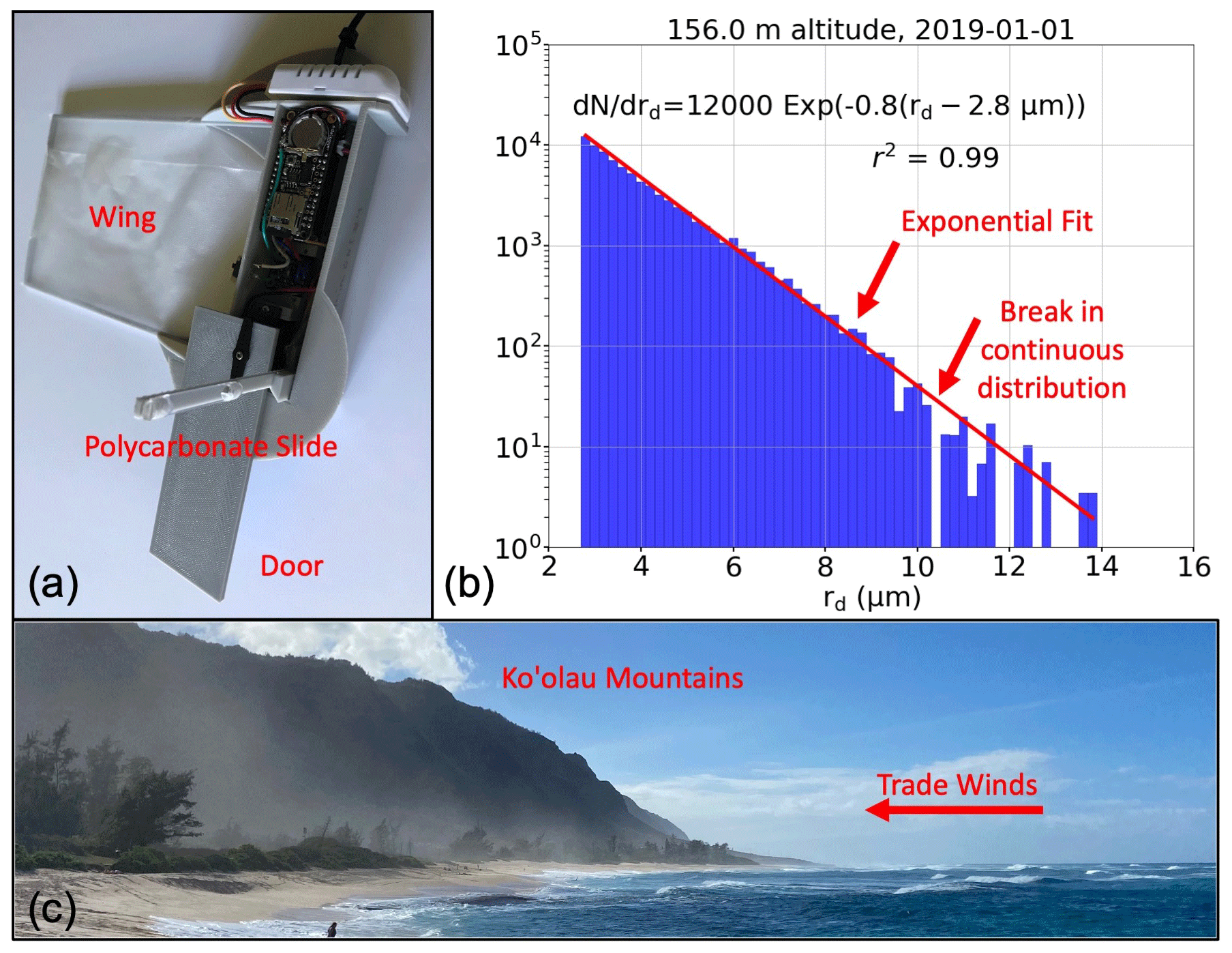
Figure 1 (a) A mini-GNI instrument is shown in its open position with the clear polycarbonate slide exposed. The door swivels shut to protect the slide from collecting SSPs during transit, while the wing covered with a thin plastic sheet helps keep the slide perpendicular to the wind during flight. The T and P sensors are within the body of the instrument, while the RH sensor is pictured outside the body on the top of the instrument. (b) An example SSA-SD from 1 January 2019 at 156 m altitude is shown. The red line shows the exponential fit, fitted with Eq. (1), and an r² value to show how well this fit represents the observed size distribution. The exponential fit is fitted up to the break in continuous SSA-SDs (up to 10.2 µm). (c) A photo of the Ko`olau Mountains with coastal SSP generation in the foreground. The trade winds are blowing onshore, bringing open-ocean and coastally generated SSPs towards the mountains, which are rapidly lifting them.

Calculations of collision efficiency (CE) are dictated by two factors: the relative air speed the slide experiences during sampling and the size of the deliquesced SSP. For all land-based samples within this study, the mini-GNI is deployed on a stationary system, meaning the relative wind speeds are the true wind speeds at that altitude and geographic location. When the mini-GNI is deployed on a nonstationary system (i.e., a moving boat), the relative wind is based on the true wind and the moving system's motion. The mini-GNI can orient itself parallel to the wind stream, thereby keeping the slide perpendicular to the wind direction and maximizing the CE. The weakest wind observation dictates which particle sizes can be compared across samples, and only particles with a collision efficiency of > 40 % are used for analyses. The weakest observed wind speed at altitude for samples in this study is 5.6 m s⁻¹, meaning that the smallest observable particle has r_d=2.8 µm. Full details on CE calculations can be found in Taing et al. (2021).

Due to the high hygroscopic nature of SSA, the RH of the environment also plays a significant role in the CE of particles. Higher RH results in greater condensational growth of SSPs, giving them larger radii, mass, and inertia than SSPs of the same dry radius at lower RH. In situ measurements of RH, T, and P from the mini-GNI are used to convert a deliquesced SSP to r_d, while calculated wind speeds aloft (see Sect. 2.3.2) are utilized for the CE. Lewis and Schwartz (2004, p. 53) consider RH to be the most significant variable in SSP growth. This study assumes the growth of SSPs is analogous to the growth of pure NaCl particles (Lewis and Schwartz, 2004, p. 54) and that these SSPs have reached their equilibrium radius (Taing et al., 2021).

After collection, the aerosol slides are analyzed using the microscope methods detailed in Jensen et al. (2020). The resulting SSA-SDs are fit with an exponentially decreasing function using the least-squares fit method of $\ln (\mathrm{d}N/\mathrm{d}{r}_{\mathrm{d}})$ to r_d (Taing et al., 2021). Here, a modified form of this equation is used:

$$\begin{array}{}\text{(1)}& {\displaystyle \frac{\mathrm{d}N}{\mathrm{d}{r}_{\mathrm{d}}}}\left(r_{\mathrm{d}}\right)=r_{\mathrm{2.8}}{e}^{-B\left(r_{\mathrm{d}}-\mathrm{2.8}\mathrm{\mu }\mathrm{m}\right)},\end{array}$$

where dN(r_d) $/$ dr_d is the concentration (N, m⁻³ µm⁻¹) at the bin (width 0.2 µm) centered on the dry-particle radius (r_d). The number concentration (r_2.8, m⁻³ µm⁻¹) is for a dry particle with a radius of 2.8 µm, which is the smallest observable SSP size in this study. Because the function is fit across a range of dry particles valid for SSPs of r_d ≥ 2.8 µm and visualized on a lognormal Y axis, r_2.8 represents the Y intercept for a given SSA-SD. The second changing parameter is B, which is the inverse of the characteristic radius for the size distribution with B>0. The lognormal Y axis represents the exponential decay equation into a linear line, meaning B represents the slope of a SSA-SD on a lognormal Y axis.

Both r_2.8 and B become the two SSA-SD shape parameters that change between SSA-SDs for different altitudes and environmental conditions and are analyzed further in this study. The inclusion of −2.8 µm in the exponent is implicit in the remainder of the equations used in this study due to the sampling range limitations. This function was fit to each size distribution from 2.8 µm through the largest-sized particle for continuous bins; i.e., the function stops fitting to particles when there is a break in the observed SSP bins (Fig. 1b). These exponential fits are then used in this study to represent the SSA-SDs for given samples if the r² values of the fits are > 0.90.

2.1.2 Coastal SSA-SDs (COAST) samples

A ground-based kite platform (Taing et al., 2021, Fig. 1a) sampled SSA-SDs along the eastern coast of O`ahu at Kaupō Bay (21<sup>∘</sup>18<sup>′</sup>54<sup>′′</sup> N, 157<sup>∘</sup>39<sup>′</sup>43.2<sup>′′</sup> W; Fig. 2). The kite platform was set up approximately 33 m inland from the shore break and 4 m above the mean sea surface elevation. At this location the trade winds blow onshore, lofting the kite along the southern portion of the Ko`olau mountain range (Fig. 2). Every deployment utilized three to five mini-GNIs to simultaneously sample at different altitudes as well as two iMet XQ2 instruments: one just below the kite and the other on the ground surface to measure P, T, and RH (InterMet, 2017). A Kestrel 5500 weather station determined preliminary wind speeds for the day and recorded approximate 2 m wind speeds throughout sampling (Kestrel Instruments, 2015). The individual SSA samples (n=77) were observed on 11 different days over an approximately 1-year period (December 2018–September 2019) and occurred on days with moderate (3–8 m s⁻¹) onshore trade winds (Table 1). Additional details on the collection methods and processing can be found in Taing et al. (2021).

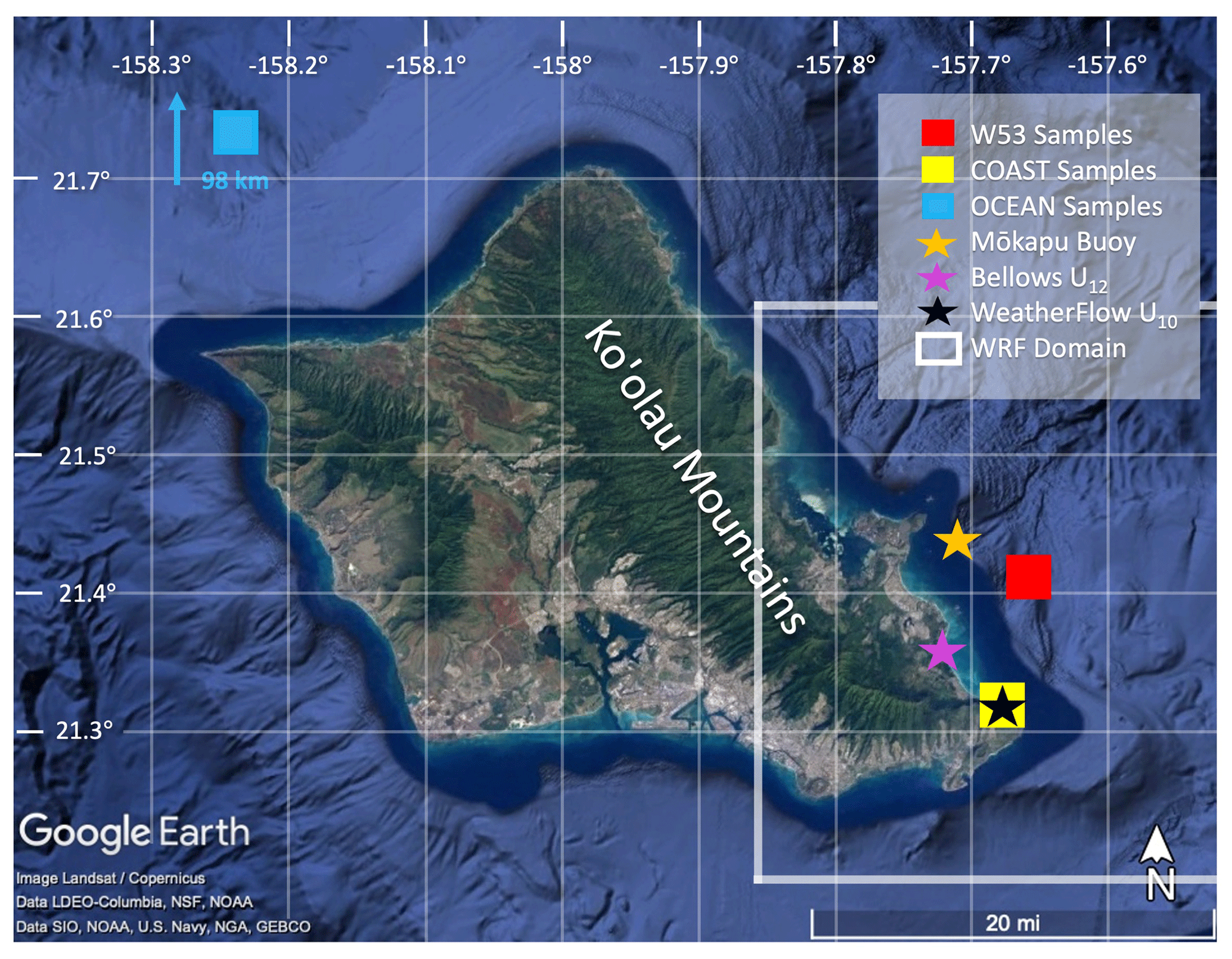
Figure 2 Sampling and data locations are marked on a map of O`ahu. The samples from the open-ocean cruise (OCEAN) were taken 98 km north of the western tip of O`ahu marked by the blue square, while the coastal samples (COAST) were taken within the yellow square at Kaupō Bay. The W53 samples are estimated to come from the region around the red square based on diagrams in Woodcock (1953). The wave state information came from the Mōkapu buoy (orange star), while wind data came from Bellows Beach (purple star) and WeatherFlow's Makapu`u beach anemometers (black star). The WRF domain is approximated by the white box but extends further to the south and east than this image. The base image is from NOAA, used under a license from © Google Earth.

2.2 Open-ocean SSA samples

2.2.1 Open-ocean SSA-SDs (OCEAN) samples

Using the same kite methodology as the coastal samples, the kite platform was deployed aboard Hawaiian Oceanographic Time-series (HOT) cruise no. 309 to collect open-ocean SSA samples. The HOT cruise utilizes the RV Kilo Moana and travels to station ALOHA approximately 98 km due north of the westernmost point of O`ahu (Fig. 2) in approximately 4 km deep water. During transects to, from, and around station ALOHA, a total of eight samples was collected from 80 to 240 m altitudes across three separate days (Table 1).

2.2.2 Historical samples

Historical open-ocean SSA-SDs collected over the ocean from Woodcock (1953) were reconstructed for comparison to samples in this study. Woodcock (1953) used a similar impaction method to the mini-GNI, exposing several slides from an aircraft at a variety of altitudes northeast of Kaupō Bay, O`ahu (Fig. 2). The SSA-SDs were plotted as inverse cumulative concentrations (N_c) along with records of the sampling day's wind force, which is a qualitative measurement of wind speed and sea state based on the Beaufort wind scale. The wind force values were converted to approximate U₁₀ wind speed ranges (Britannica, 2023), and the N_cs from Fig. 1 in Woodcock (1953) were converted from a formation radius size at 99 % RH to r_d for comparison to this study. All further references to samples from Woodcock (1953) will be referred to as W53.

2.3 Environment data

2.3.1 Sea state

Sea state data like significant wave height (H_s) and SST came from the Pacific Islands Ocean Observing Systems (PacIOOS) Mōkapu buoy (Coastal Data Information Program, 2000) located 4.5 km offshore of the windward coastline at a water depth of 86 m (Fig. 2). Depending on the swell conditions, this buoy represents intermediate to deep water waves, with the average wave height to wavelength ratio maintaining a deep water wave classification. This buoy remains the closest geographically to Kaupō Bay and represents approximate open-ocean sea state conditions for the eastern portion of O`ahu.

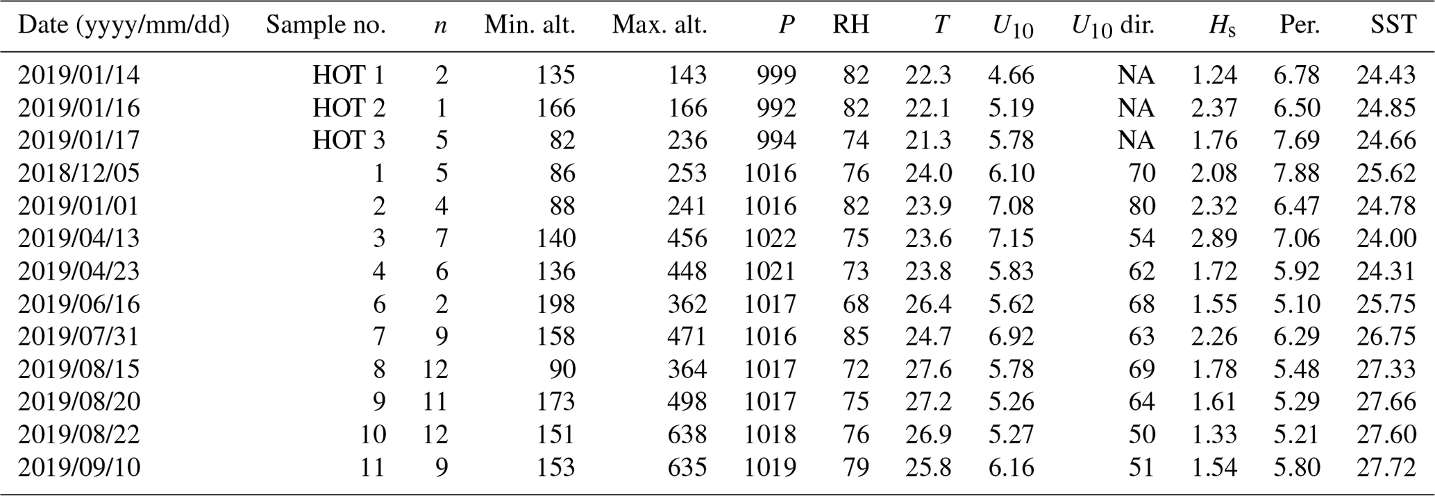
Table 1 Totals of 77 coastal samples from 10 sampling days and 8 open-ocean samples from 3 sampling days (HOT) were utilized in this study. Altitudes range from 86 to 638 m. Sampling date (yyyy/mm/dd), sample number, number of samples taken on each sampling date (n), minimum and maximum sampling altitude (m), and averaged values of surface P (hPa), RH (%), T from samples (^∘C), U₁₀ (m s⁻¹), U₁₀ wind direction (^∘), H_s (m), mean wave period (Per., s), and SST (^∘C) are shown in the table. Sampling date no. 5 was not included in this analysis as the altitudes of all the samples were < 80 m. For atmospheric state variables, the averages are taken across all the sampling altitudes recorded by each mini-GNI for the duration of sampling except for surface pressure, while ocean variables are averaged across the sampling duration from their collection locations. Wind direction was not available (NA) for the three open-ocean samples.

2.3.2 U₁₀ calculations

In February 2020, a private 10 m anemometer was installed at Kaupō Bay by WeatherFlow (R. M. Young Company, 2016), approximately 5 months after the completion of SSA sampling. A linear regression on almost 2 years' worth of data was conducted between wind speeds measured by a 12 m anemometer at Bellows Beach, approximately 7 km northwest of Kaupō Bay (Bellows U₁₂, Fig. 2) and a 10 m anemometer at Mapakpu`u Beach (WeatherFlow U₁₀, Fig. 2) for trade wind days only (wind directions between 30 and 90^∘). Pearson's r between these two locations was 0.904 and significantly better correlated than our in situ 2 m Kestrel samples with Bellows U₁₂ (Pearson's r=0.681). Therefore, a relationship between WeatherFlow U₁₀ and Bellows U₁₂ was derived to approximate historical wind speeds for the SSA sampling dates.

Finally, following the methodology from Taing et al. (2021), wind speeds (u(z)) at the sampling altitudes aloft (z) were calculated using WeatherFlow U₁₀ wind speeds (u_r(z_r)) applied to a logarithmic dependence of wind speed with altitude from Arya (2001).

$$\begin{array}{}\text{(2)}& {\displaystyle \frac{u\left(z\right)}{u_r\left(z_r\right)}}={\displaystyle \frac{\ln \left(z/z_{\mathrm{0}}\right)}{\ln \left(z_r/z_{\mathrm{0}}\right)}}\end{array}$$

The assumed surface roughness length (z₀) was 0.001, consistent with coastal location measurements (Arya, 2001). These wind speeds were then used to calculate the CE for all SSA particle sizes as well as the total air volume sampled. For this paper, any reference to U₁₀ wind speeds for coastal SSA samples will be to these calculated wind speeds for the Kaupō Bay area.

2.3.3 Vertical environment profiles

For every kite deployment, an iMet XQ2 instrument was attached approximately 25 m below the kite. The iMet XQ2 samples T, P, RH, geographic position (latitude, longitude), and altitude (z) at 1 Hz frequency for the entire sampling duration of 2–3 h. Vertical profiles of the environment were collected during the kite ascent and descent, which occurred approximately three times per sample date. T, RH, and P were averaged 1 m altitude increments for the sampling period and used to calculate the terminal fall velocities of six different SSPs as they change with altitude and changing environmental conditions.

2.4 SSP trajectory modeling

2.4.1 Weather Research and Forecasting (WRF) model setup

The WRF model V4.0 provided wind field estimates across a high spatial resolution for two sampling days in this study (Skamarock et al., 2019). Only u, v, and w speeds were utilized from these simulations to supplement wind information for a high-resolution three-dimensional fluid flow over complex terrain. A single square domain was chosen from 21^∘36^′49^′′ N, 157^∘52^′5.52^′′ W to 21^∘11^′9.92^′′ N, 157^∘24^′47.16^′′ W, resulting in 250 by 250 grid points with 200 m horizontal resolution (Fig. 3a). The domain was forced with the National Centers for Environmental Prediction (NCEP) 1^∘ Model Global Tropospheric Analyses with custom 200 m topography to realistically represent updraft velocities created by the steep orographic gradients of the Ko`olau Range. Additionally, custom η values, or pressure-derived height values, were chosen for the lower portion of the atmosphere, with the lowest 1.5 km represented by approximately 40 m vertical levels, followed by 100 m vertical levels through 5 km. The Thompson microphysics scheme was used (Thompson and Eidhammer, 2014) along with a rapid radiative transfer model for longwave and shortwave radiation and the Shin and Hong (2015) planetary boundary layer scheme. The diffusion option was evaluated in physical space (stress form), and horizontal Smagorinsky first-order closure was used to compute the K coefficient. Because the terrain slopes are >45^∘ in some regions, the time off-centering parameter was tuned to dampen vertically propagating sound waves and prevent model errors. Other namelist parameters were in agreement with National Center for Atmospheric Research recommendations for WRF runs with grid spaces between 100 m and 1 km.

Two simulations were completed based on wind data from our sampling dates: one relatively high-wind-speed day (HW, 31 July 2019) with a 7 m s⁻¹ average in situ U₁₀ and one relatively low-wind-speed day (LW, 22 August 2019) with a 5 m s⁻¹ average in situ U₁₀. After approximately 24 h of model spinup time, a vertical transect was taken perpendicular to the coastline (Fig. 3a), where the u, v, and w fields were averaged for 3 h for our in situ sampling period (Fig. 3b and c). For the total space of the transects, the high- (low)-wind simulation had an average updraft speed of 0.40 m s⁻¹ (0.22 m s⁻¹), an average u component of −8.54 m s⁻¹ (−5.34 m s⁻¹), and an average v component of −5.68 m s⁻¹ (−3.84 m s⁻¹). Differences in updraft speeds between these two days along the coastline varied from as little as 0.1 m s⁻¹ to over 1.5 m s⁻¹.

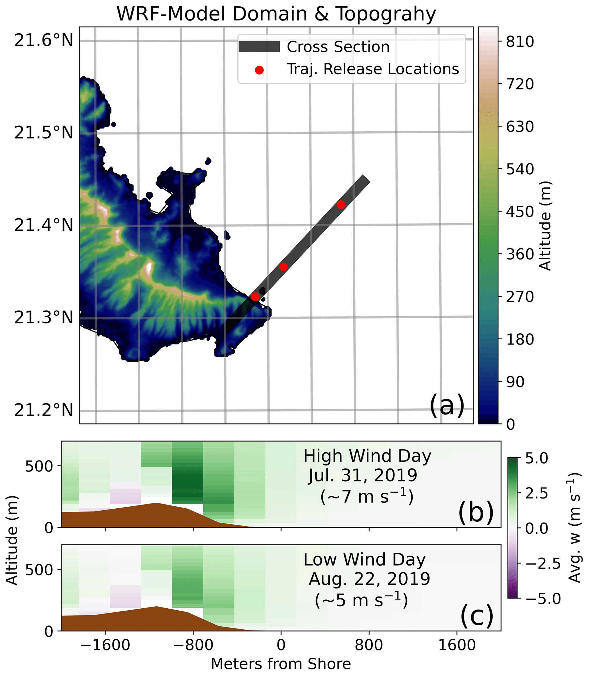
Figure 3 (a) The complete WRF domain is shown with the topography of the Ko`olau Range. The black line represents the 3 h averaged vertical cross section taken for plots (b) and (c), and the red dots represent the production locations for the trajectories in Sect. 6. The average simulated vertical velocities (w) within the cross section are shown on a (b) high-wind day (an average u−v component of 7 m s⁻¹ observed in situ) and a (c) low-wind day (an average u−v component of 4 m s⁻¹ observed in situ) for comparison.

2.4.2 SSP fall velocity calculations

Fall velocities that include hygroscopic particle growth with altitude were calculated for variously sized GSSPs. The fall velocities (v_∞) utilized equations from Table 1 in Beard (1976) with the addition of dry salt mass for each GSSP, as the original equations treated the falling droplets as pure water. The fall velocities for six GSSPs (r_d=2.8, 5.0, 7.4, 9.8, 12.2, and 15.6 µm) were calculated from the surface through the cloud base at 1 m increments using the averaged vertical profiles from the iMet XQ2 for the high- and low-wind days. Reference to these six particle sizes will be in the form r_d, followed by a subscript of their dry particle size in microns, e.g., r_d2.8, and they are not to be confused with the concentration variable r_2.8 defined in Sect. 2.1.1. Figure 4 shows how particle growth and fall velocities change with altitude for the low-wind day (22 August 2019). Altitude is effectively an analog for RH in this case, as the observed RH profiles with altitude were approximately linear for both days. The condensational growth equation from Lewis (2008) shows the hygroscopic growth of an SSP given its dry radius and RH:

$$\begin{array}{}\text{(3)}& r_{\mathrm{RH}}=\mathrm{1.08}{r}_{\mathrm{d}}\left(\mathrm{1.1}+{\left({\displaystyle \frac{\mathrm{1}}{\mathrm{1}-\mathrm{RH}+{\left(\frac{\mathrm{1.1}\times {\mathrm{10}}^{-\mathrm{9}}}{\mathrm{1.08}{r}_{\mathrm{d}}}\right)}^{\frac{\mathrm{3}}{\mathrm{2}}}}}\right)}^{\frac{\mathrm{1}}{\mathrm{3}}}\right),\end{array}$$

where r_RH is the deliquesced particle size at that relative humidity. Because the RH remains ≥ 70 %, we assume that the GSSPs are spherical to remove complications created by amorphous droplet shapes.

2.4.3 SSP trajectory calculations

Lastly, trajectories for GSSPs sized r_d2.8, r_d7.4, and r_d12.2 were simulated using the 3-hourly averaged WRF wind profiles around the average time for our in situ samples (14:00 local time) as well as the calculated fall velocities from both wind days. Three production locations (represented by the red dots in Fig. 3: 100 m (“Coastline”), 2600 m (“Intermediate Zone”), and 5800 m (“Open Ocean”) offshore) were chosen to study how distance from the coastline affects each particle size's horizontal and vertical mixing potential on the high- and low-wind days. One hundred trajectories were run for every particle size, production location, and wind speed day, resulting in a trajectory range for each scenario (Fig. 11). GSSPs were released between 10 and 25 m, decreasing exponentially with altitude from 10 m, in agreement with observations from Gathman and Smith (1997), Hooper and Martin (1999), and Porter et al. (2003). Because the GSSPs were released at 10 m and above, we assume they are already in equilibrium with the ambient RH (Lewis and Schwartz, 2004).

As the GSSPs moved throughout the domain, the trajectory was tracked until the particle reached sufficiently past our kite sample location or when the particle reached an altitude of 0 m, for which we assume the GSSP has been removed from the atmosphere via dry deposition. Stochastic variation within 2 standard deviations of the WRF wind simulations was introduced to each trajectory's u, v, and w fields at each time step, with each deviation chosen based on the probabilities of that deviation given a Gaussian distribution centered on the average speed for each wind component. These variations were designed to represent the real-life expected natural variability in the wind field.

Trajectories, therefore, account for the growth in deliquesced SSP radii based on RH changes with altitude, consequent change in v_∞ from changes in atmospheric state variables with altitude, and the pseudo-natural variation of u, v, and w speeds at all particle positions. The average maximum altitude (AMA) was then calculated for all particles for each production location and wind speed day to represent the relative differences in altitude achieved by these trajectories. The AMA, however, is artificially limited by choosing to evaluate an area close to the kite sampling and does not represent the total potential altitude range these particles may reach beyond the domain in this study.

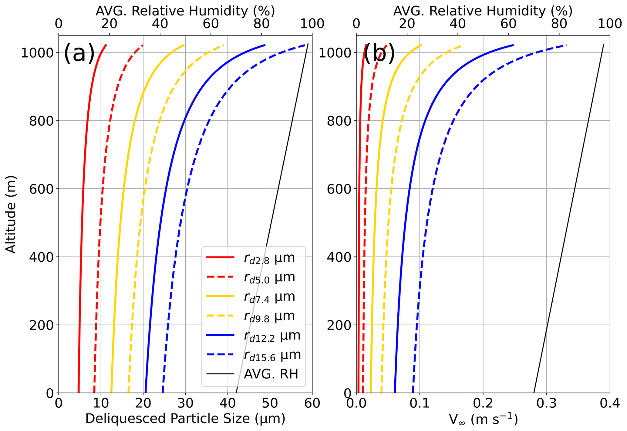
Figure 4 The (a) deliquesced particle radius (µm) and the resulting (b) terminal fall velocity (v_∞, m s⁻¹) for six GSSPs are shown, color-coded and with alternating solid and dashed lines by their r_d for the low-wind day (22 August 2019). The hygroscopic growth shown in panel (a) utilizes the average iMet XQ2 RH vertical profile (black line) from the sample date to show how GSSPs grow as they ascend from the surface up to the cloud base at 1050 m. The radii more than double from the average surface RH (68 %) to just below the cloud base (98 %), and the mass of the deliquesced SSPs grows approximately 4.5 times in size. The calculation of the terminal fall velocity combines the changes in mass, radius, and atmospheric state variables with altitude.

3 COAST vs. OCEAN

3.1 Averaged SSA-SDs on the coast vs. in the open ocean

To assess the impacts of the coastline on SSA-SDs, this study compared COAST and OCEAN within the same U₁₀ (3.4–6.3 m s⁻¹) and altitude (80–240 m) ranges. U₁₀ is largely considered the dominant factor in open-ocean SSA production, either indirectly through the generation of whitecaps or directly through spume droplet production at higher wind speeds (De Leeuw et al., 2011). At the smallest observable r_d, COAST concentrations (m⁻³ µm⁻¹) are approximately 2.7 times higher than OCEAN concentrations (m⁻³ µm⁻¹). As r_d increases, average COAST GSSP concentrations gradually increase to 5.2 times greater than average OCEAN concentrations (Fig. 5), resulting in a slight decrease in B between the OCEAN and COAST samples. This decrease in B also illustrates that the average COAST sample has a larger total range of GSSP sizes, approximately 2 µm larger, than the average OCEAN r_d range.

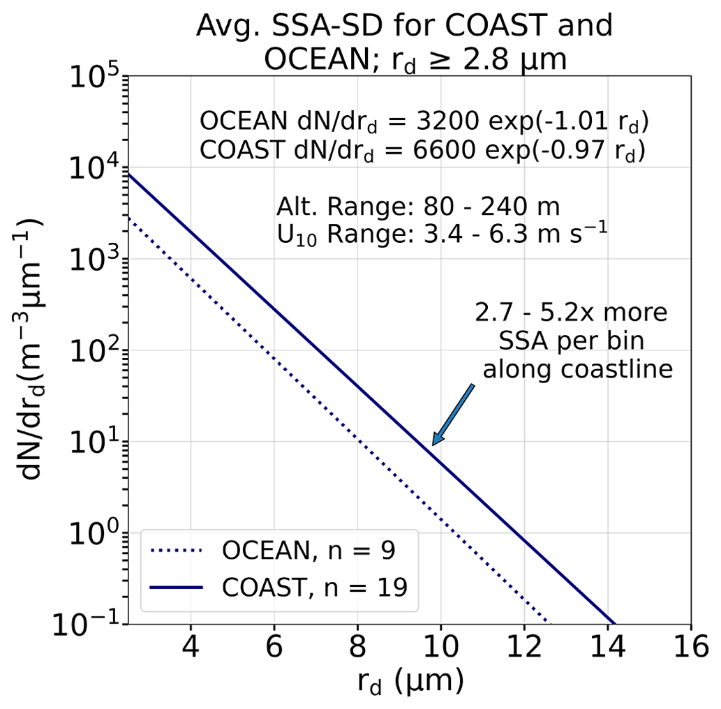
Figure 5 Altitude- and environment-averaged SSA-SDs are plotted for samples taken from the windward coastline (COAST, solid blue line) and the open ocean (OCEAN, dotted blue line) north of O`ahu. Both SSA-SDs contain samples between 80 and 240 m altitude and between 3.4 and 6.3 m s⁻¹ wind speeds. The COAST sample has more GSSPs at all observable radii, with a larger multiplying factor as GSSP radii increase. This is also echoed in the COAST size distribution function (dN $/$ dr_d), which has a larger r_2.8 value and less steep slope when compared to the OCEAN size distribution function.

3.2 Cumulative concentrations vs. historical W53

The OCEAN samples were limited in number and environmental variety, so historical SSA-SDs measured during the 1950s by Woodcock (1953) were used to compare samples over a greater range of observations. For the 3.4–5.4 m s⁻¹ U₁₀ range, the average OCEAN N_c remains close to W53 N_c (Fig. 6a), demonstrating that OCEAN samples in this study are well matched to historical open-ocean observations. For COAST observations, however, N_cs in both U₁₀ ranges exceed the W53 N_cs. Furthermore, the COAST samples only observed wind speeds up to 7.9 m s⁻¹ and still have a larger N_c than W53, which has a total wind speed range of up to 10.4 m s⁻¹. Additionally, the difference between COAST N_cs and W53 N_cs remains consistent at all GSSP radii, indicating that COAST samples in this study have a greater concentration of all GSSP sizes.

Next, two W53 N_cs at discrete altitudes (561 and 518 m from Figs. 3 and 4 in Woodcock, 1953) and U₁₀ ranges were compared to averaged COAST samples at similar altitudes and U₁₀ ranges (Fig. 6b). Only two samples from Woodcock (1953) were useful for this comparison, as they were the only two discrete samples in Hawai`i confirmed to be below the cloud base. Sampling above or below the cloud base is an important distinction due to recent findings that SSA concentrations taken above the cloud base do not correlate well with changes in environmental conditions like wind speeds above the ocean's surface (Zheng et al., 2011). The COAST samples lack observations between 498 and 614 m, and therefore averaged N_cs were calculated for samples taken between 450 and 638 m. Overall, COAST N_cs are greater than W53 N_cs for both the 3.4–5.4 and 5.5–10.4 m s⁻¹ U₁₀ ranges. For the stronger U₁₀ range, the COAST N_c remains larger than W53 despite lacking observations for U₁₀ for the upper range observed in W53 (7.9–10.4 m s⁻¹). Unlike Fig. 6a, these upper-altitude COAST samples converge on W53 samples as r_d decreases. We hypothesize that the coastline observes greater vertical mixing of larger GSSPs than found over the open ocean at these altitudes and that concentrations of smaller GSSPs aloft are more similar to open-ocean observations. These differences may be due to the negligible updraft speeds required to mix a 3 µm GSSP vs. those required of an ultragiant SSP (Fig. 4b).

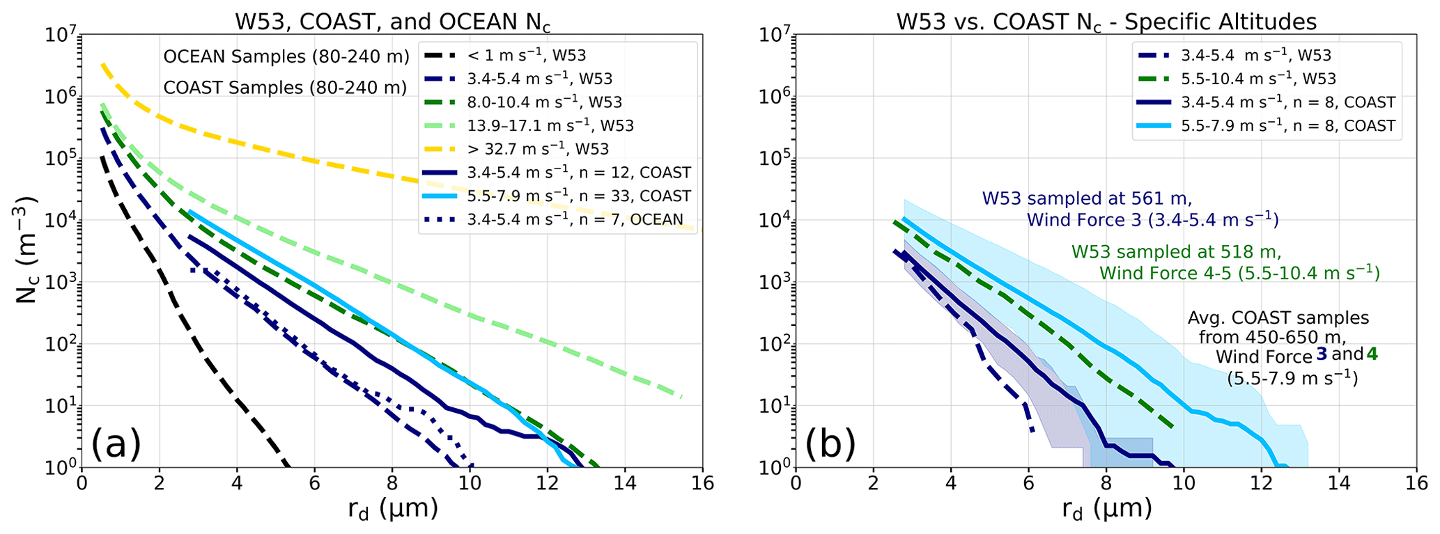
Figure 6 Inverse cumulative concentrations (N_c) were used to compare how concentrations of SSA change from the largest to the smallest observable SSA bin (r_d ≥ 2.8 µm). Plot (a) shows the averaged cumulative concentrations measured by W53 (dashed lines) for discrete wind speed ranges, with our COAST (solid lines) and OCEAN (dotted line) samples for the same altitude range (80–240 m). Plot (b) shows two specific W53 samples at discrete altitudes (561 and 518 m from Figs. 3 and 4 in Woodcock, 1953) and wind ranges to averaged COAST samples for the same altitude and similar U₁₀ ranges. The shaded regions show the range between the smallest and largest COAST N_c within each U₁₀ range.

4 Environmental dependencies of COAST SSA-SDs

4.1 SSA-SDs and environmental variables

SSA production and subsequently atmospheric concentrations of SSA are intrinsically tied to interactions between the air and sea. To understand how the environment impacts the natural variability of SSA, SSA-SDs were plotted for the complete range of U₁₀ and H_s observed in this study (Fig. 7). The color of each size distribution represents discrete values for both environmental variables – the more organized the color spectrum is, the more correlated SSA-SDs are with changes in that environmental variable. There are strong positive correlations between the organization of SSA-SDs and both U₁₀ and H_s: as U₁₀ and H_s increase, the overall concentrations and slope of the SSA-SDs become gentler, indicating higher concentrations of GSSPs and a wider range of GSSPs with increases to both environmental variables. SSA-SDs organized by U₁₀, however, appear to have slightly higher variability than H_s.

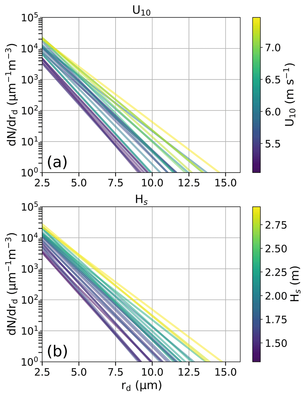
Figure 7 SSA-SDs were binned and averaged by two environmental parameters – (a) U₁₀ (m s⁻¹) and (b) H_s (m) – to visualize the organization of these size distributions to changes in the wind and waves. SSA-SDs show a strong positive organization to U₁₀ and H_s.

4.2 SSA-SD shape parameters by U₁₀ and H_s

To further investigate these relationships' specific impacts on SSA-SD shape parameters, r_2.8, B, and the cumulative concentrations of ultragiant SSPs (y₁₀, r_d > 10 µm) were plotted and color-coded by the average value of U₁₀ and H_s for each sample (Fig. 8). Every subfigure in Fig. 8 shows a moderate to strong visual correlation between the SSA-SD shape parameters U₁₀ and H_s. Given the high correlation between U₁₀ and H_s (Pearson's r=0.85), partial correlations determine the linear dependence between SSA-SD shape parameters and U₁₀ or H_s while isolating the influence to only one environmental variable. The partial correlation is therefore calculated as

$$\begin{array}{}\text{(4)}& {\mathit{\rho }}_{ab.c}={\displaystyle \frac{r_{ab}-r_{ac}{r}_{bc}}{\sqrt{\mathrm{1}-{r_{ac}}^{\mathrm{2}}}\sqrt{\mathrm{1}-{r_{bc}}^{\mathrm{2}}}}}.\end{array}$$

Variable a is any of the three SSA-SD shape parameters, while variables b and c are U₁₀ and H_s, respectively, for correlations isolating the relationship with U₁₀ and the inverse when isolating the relationships with H_s. Therefore, r_bc is always Pearson's r correlation between U₁₀ and H_s, which is 0.85 for this study. The other two Pearson's r correlations, r_ab and r_ac, represent the correlation between the two subscripted variables, and ρ_ab.c represents the partial correlation between variables a and b without the controlling variable c.

Figure 8a and b show moderately positive correlations between r_2.8 and B. Positive correlations are also seen between r_2.8, B, and environmental variables and maintain strong Pearson's r correlations (Table 2). When partial correlations (ρ) are applied, however, the correlation between U₁₀ and r_2.8 is reduced to a moderate correlation, while the partial correlation between H_s and r_2.8 remains strong. The differences in partial correlations indicate that the majority of the environmental correlation with r_2.8 belongs to changes in H_s rather than U₁₀ and that the initial strength of the Pearson's r value between r_2.8 and U₁₀ may come from the inherent relationship between U₁₀ and H_s in this study. A more drastic pattern emerges with B, where the partial correlation between H_s and B becomes stronger, while the partial correlation between U₁₀ and B is entirely removed. B sets the shape of the SSA-SD, meaning a good SSA production equation should be represented by an environmental variable that captures changes in not only concentration, but also the concentration changes across different radius bins. Both of these partial correlations support H_s being a stronger environmental control than U₁₀ on coastal SSA-SD shape parameters.

Table 2 The U₁₀ Pearson's r, H_s Pearson's r, ${\mathit{\rho }}_{U_{\mathrm{10}}}$, and ${\mathit{\rho }}_{H_{\mathrm{s}}}$ are shown for SSA-SD parameters r_2.8, B, and y₁₀. The ${\mathit{\rho }}_{U_{\mathrm{10}}}$ is the partial correlation of these variables with U₁₀ in the absence of H_s, while ${\mathit{\rho }}_{H_{\mathrm{s}}}$ is the partial correlation of these variables with H_s in the absence of U₁₀. Bold values indicate strong positive correlations.

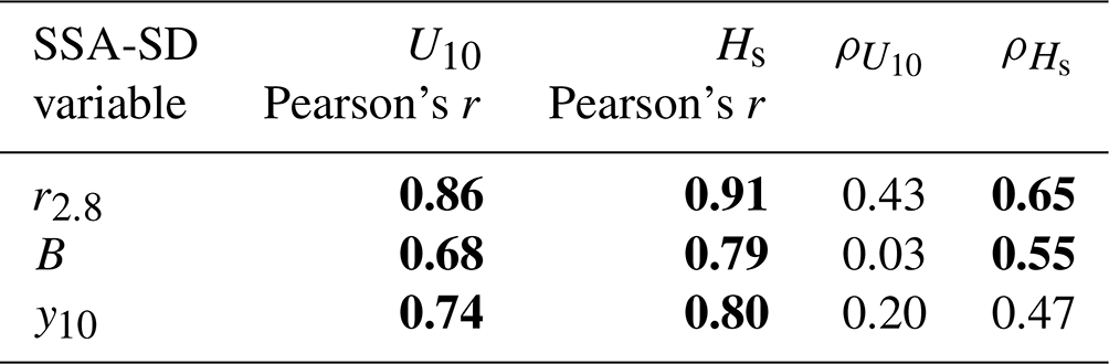
Another important aspect of an SSA-SD's correlation with the environment is the ability to accurately predict y₁₀. As seen in Sect. 3, COAST SSA-SDs show a larger increase in y₁₀ concentrations than smaller GSSPs when compared to OCEAN SSA-SDs, hinting that production processes for ultragiant SSPs may differ from the coast to the open ocean. However, capturing these changes in a fitted distribution can be difficult because the shape parameters are more likely to be set by the smaller-sized, more plentiful SSPs. Therefore, analysis of y₁₀ to both U₁₀ and H_s highlights whether SSA-SD shape parameters accurately represent the ultragiant SSPs in this study. Figure 8c and d show the dependence of y₁₀ on B influenced by U₁₀ and H_s, respectively. Minimal differences in scatter distribution shapes emerge, and both U₁₀ and H_s have strong Pearson's r correlations with y₁₀ (Table 2).

Similar to Fig. 8a and b, the visual correlation of y₁₀ with U₁₀ and H_s (Fig. 8c and d, respectively) differs slightly, with H_s appearing more organized than U₁₀. Partial correlations show that H_s has the strongest correlation with y₁₀, but there remains a weak partial dependence of y₁₀ on U₁₀. Because ultragiant SSPs fall within the size range for spume droplets, this wind dependence may come from offshore spume droplet production in regions where U₁₀ exceeds 9 m s⁻¹. These ultragiant SSPs have significant fall velocities; therefore, U₁₀ may play an important role in modulating not only the maximum horizontal travel distance of these ultragiant SSPs, but also their vertical transport due to changes in turbulent kinetic energy.

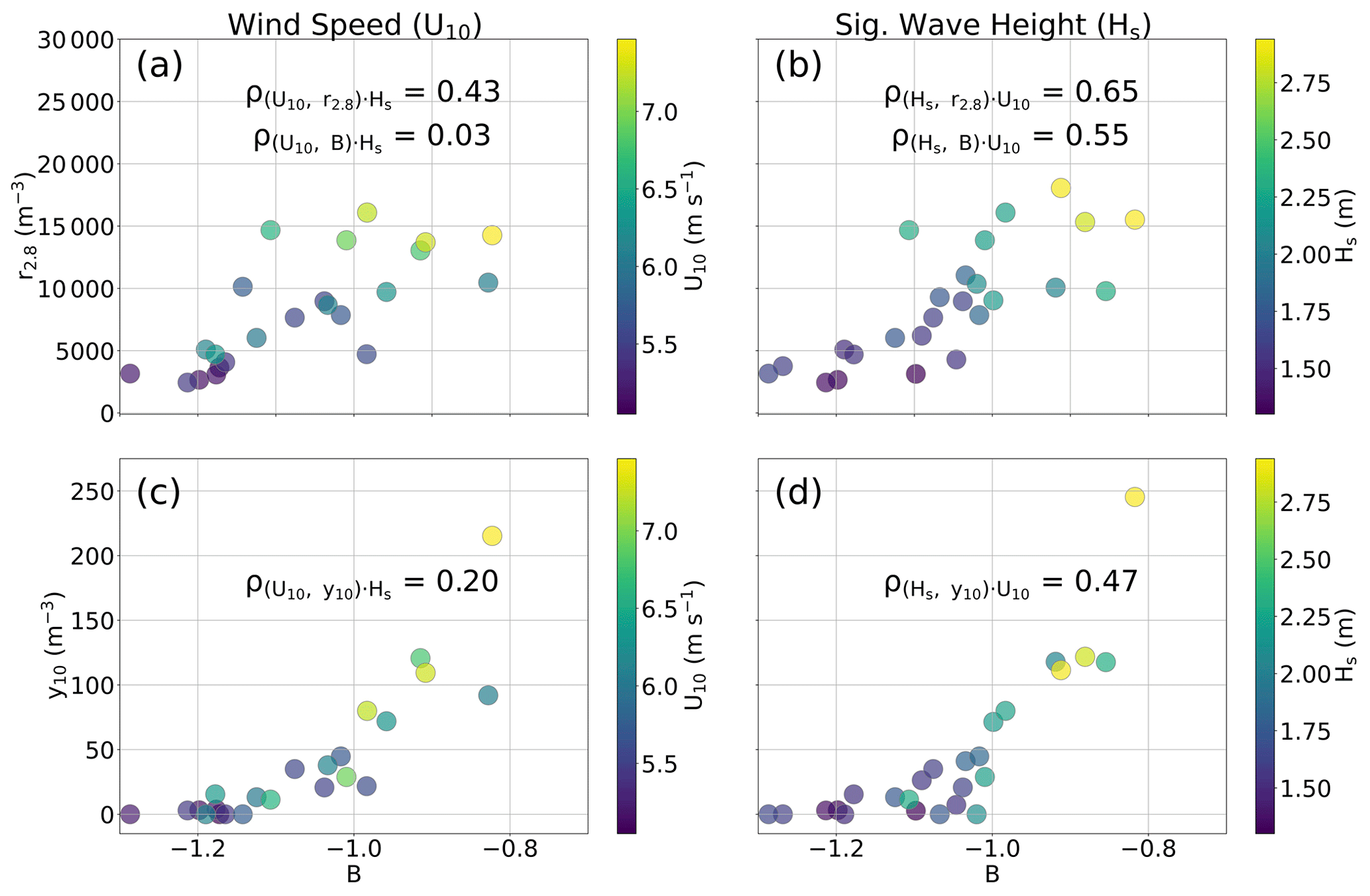
Figure 8 Three SSA-SD shape parameters are plotted: r_2.8, B, and y₁₀, which are binned and color-coded by U₁₀ and H_s. Plots (a) and (c) are binned by U₁₀, while plots (b) and (d) are binned by H_s. Shape parameter B is used for the x axis of all the plots. The partial correlations between these shape parameters and the environmental variables from Table 2 are also shown.

Exton et al. (1985)Daniels (1989)Petelski and Chomka (1996)Chomka and Petelski (1997)Piazzola and Despiau (1997)De Leeuw et al. (2000)Reid et al. (2001)Clarke et al. (2006)Van Eijk et al. (2011)Yang et al. (2019)

Table 3 This table shows a collection of historical in situ sea salt studies in coastal areas. The observed range of SSPs for each study has been converted to r_d from the study's original range. If the ambient humidity was not considered in the particle size, the formation radius (r₉₈) or 80 % RH was assumed based on the sampling altitude in the study. The measurement type, either total sea salt mass (Mass), total particle concentration (Concentration), or size distribution for the particle range (Size dist.), is recorded, along with which variable correlated most strongly with each study's observations (Sig. var.) and the dates on which the study occurred (Duration).

5 Vertical distributions of SSA-SDs

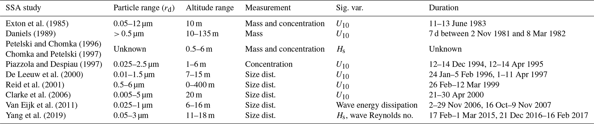
In situ coastal studies historically observed SSA within the bottom 30 m of the atmosphere (Table 3). To gain a strong quantitative understanding of SSA production, historical studies measured total mass, total particle concentration, or SSA-SDs to characterize SSA production at the air–sea interface (Table 3). Remote-sensing studies like Gathman and Smith (1997), De Leeuw et al. (2000), and Porter et al. (2003) observed that SSA production plumes can rapidly spread vertically to higher altitudes than observable by many in situ studies, meaning many in situ point-source measurements could miss a bulk of SSA production when compared to remote-sensing observations. While this study also utilizes in situ point-source measurements, simultaneous sampling at multiple altitudes provides an increased observational capacity of vertical mixing for different particle sizes as well as insight into how well upper-altitude SSA-SDs correlate with changes in their local environment.

The total average mass for four altitude bins from 80 to 640 m was calculated for each sampling day, showing minimal variability in total mass with altitude (Fig. 9a). The largest differences between samples, instead, come from the changes in environmental conditions between sampling days. Overall, the lowest three altitude bins experience a decrease in total average mass with altitude and a small decrease in total GSSP concentration, but there are several days on which total mass increases with height from the lower-altitude bins.

Masses and concentrations are difficult to interpret by themselves due to the wide range of B and r_2.8 combinations that could produce the SSA masses and concentrations observed in this study. Figure 9b shows the averaged SSA-SDs for the three main altitude bins from all the sampling days in Fig. 9a. Despite the significant v_∞ of ultragiant SSPs at upper altitudes (≥ 0.2 m s⁻¹, Fig. 4b), B, r_2.8, and total GSSP size range remain very similar with altitude and indicate that, on average, the marine boundary layer is very well mixed at our sampling location.

Lastly, two days from OCEAN and COAST with nearly identical U₁₀ and H_s values were compared to evaluate whether coastal dynamics influence SSA-SD changes with altitude (Fig. 10). Over a more limited altitude range, observations confirm similar patterns from Sect. 3. The COAST concentrations are greater than the OCEAN samples at all altitudes, and the COAST samples observe a larger total range of GSSP sizes at each altitude than the OCEAN samples. Interestingly, changes in the SSA-SD shape parameters are more significant. COAST r_2.8s increase with altitude, while OCEAN's decrease steadily with altitude. Because these sampling days have similar environmental conditions, these results strengthen the conclusion that the coast aids in increasing SSA production but do not explain why COAST samples could experience an increase in r_2.8s with altitude. We hypothesize that this increase is likely due to local dynamical controls on the vertical mixing in that region and that the fall velocities and production location in proximity to the coastline of these GSSPs may prove more important.

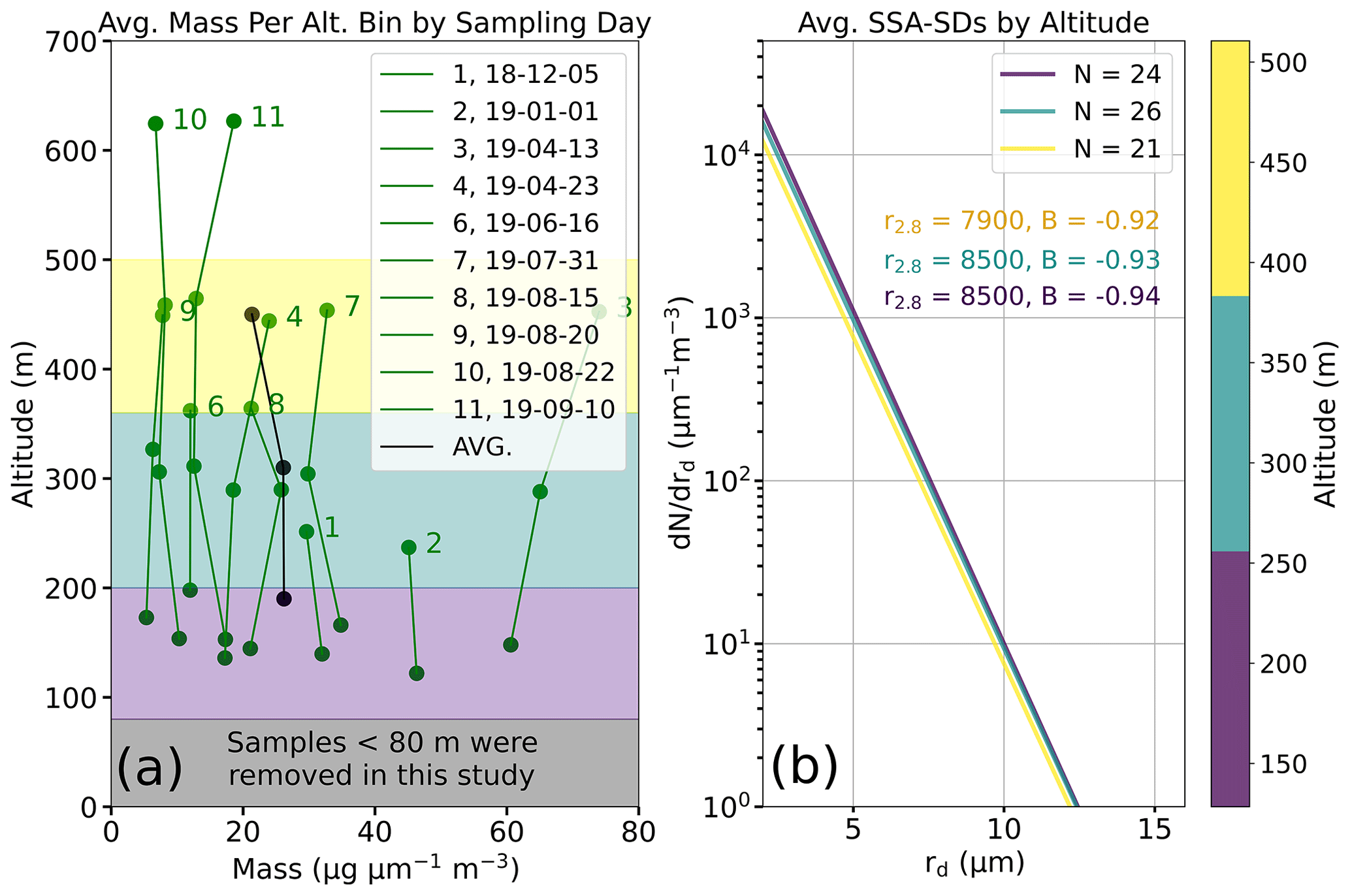
Figure 9 (a) The averaged total SSA mass for individual samples was plotted across four altitude bins: 80–200, 200–360, 360–510 m, and > 510 m for the individual sampling days. Within the three lowest-altitude bins, SSA masses were averaged across all the sampling conditions to show how samples change with altitude (black solid line). The masses for the central bins decreased with altitude (5.24, 5.22 µg m⁻³, and the highest bin 4.27 µg m⁻³). (b) The individual sample days in panel (a) from the three lowest-altitude bins were averaged together to create SSA-SDs. These depict how SSA-SDs and their shape parameters change with altitude across all the sample days rather than only mass.

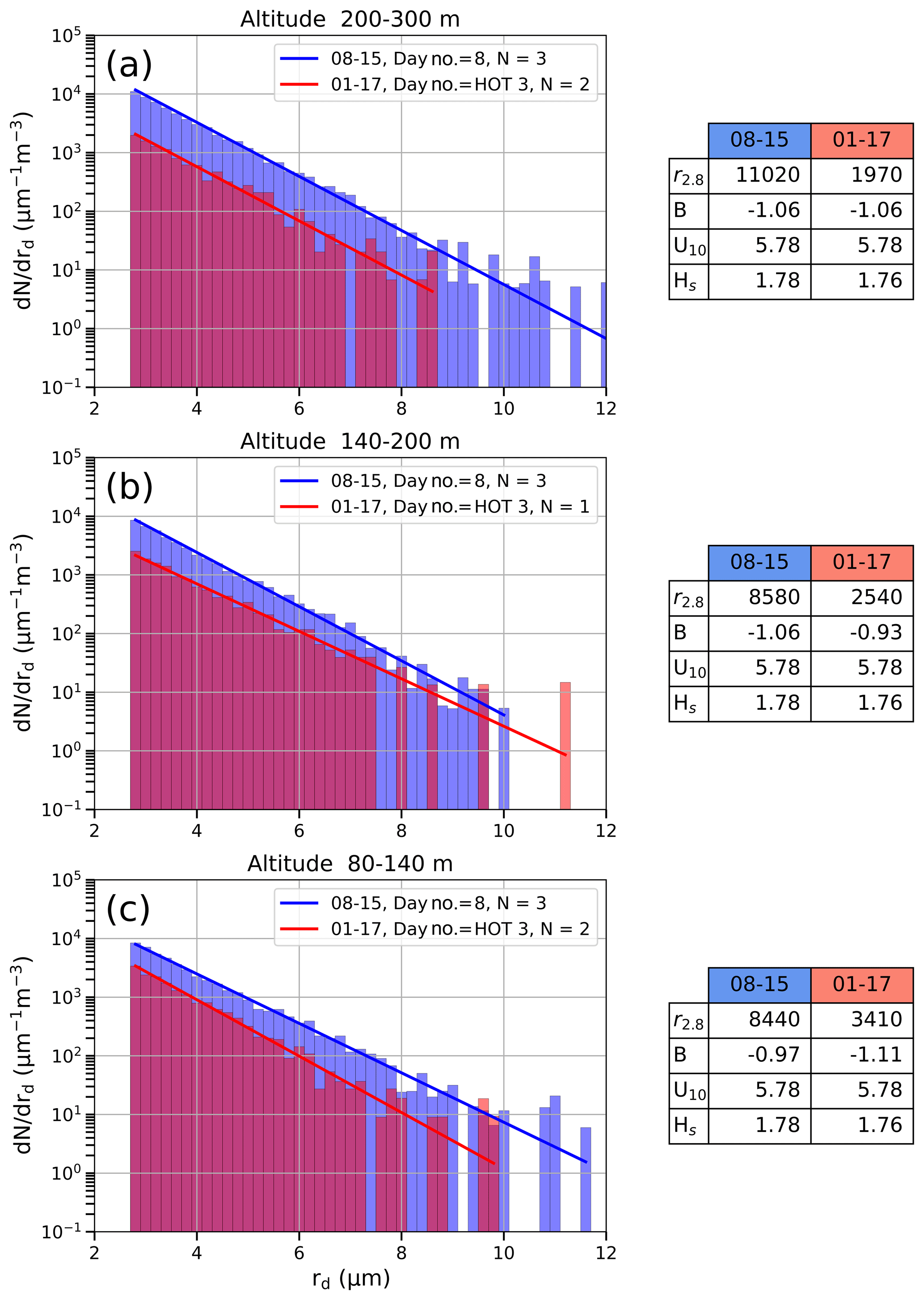
Figure 10 Two sampling dates from the OCEAN (red) and COAST (blue) with similar environmental conditions were chosen to compare changes in SSA-SDs with altitude. Three discrete altitude bins were compared based on the availability of samples between these two days. SSA-SD parameters r_2.8 and B, along with the two environmental variables U₁₀ and H_s, are shown in the tables to the right of each graph.

6 Modeling coastal orographic impacts on SSA-SDs

While we have investigated the changes to SSA-SDs between the coast and the open ocean, it is difficult to remove the influence of the open ocean on these observations. More plainly, these coastal observations likely contain a mixture of GSSPs produced in the open-ocean and coastal regions. Therefore, SSA trajectories help to supplement how the production location and environment wind speeds affect differently sized GSSPs' vertical mixing potentials.

Fall velocities from Fig. 4b show that a singular particle's v_∞ can increase significantly from the ocean surface to the cloud base. The smaller GSSPs in this study have negligible fall velocities (Fig. 4b) and can remain in the atmosphere for days to weeks, meaning their ability to travel freely through the atmosphere is limited mainly by wet deposition (Lewis and Schwartz, 2004, p. 76). The larger GSSPs remain suspended for an average of just minutes, however, meaning their ability to be vertically and horizontally mixed is more limited by their masses (Lewis and Schwartz, 2004, p. 76). As a result, larger GSSPs and ultragiant SSPs require stronger updrafts to move similar horizontal or vertical heights to their smaller counterparts. This is an overall limiting factor of atmospheric concentrations of ultragiant SSPs.

Trajectory ranges for three radii of GSSPs are shown for three production locations for the high- and low-wind days (Fig. 11). When particles were released at the Coastline production location (100 m offshore), all three GSSP radii were vertically mixed regardless of their size (Fig. 11a, d, g). A small difference in the average maximum altitude obtained in this domain (AMA) is observed between r_d2.8 and r_d12.2 for both wind simulations, and the low-wind day sees smaller AMAs across all the GSSP sizes. No GSSP size experienced dry deposition, indicating that particles released in Coastline become rapidly vertically mixed by the coastal orographic updrafts on both the low- and high-wind days.

At the Intermediate production location (2600 m offshore), all GSSPs experienced increased AMA except for r_d12.2 on the lowest wind day. The AMA for r_d12.2 decreased by almost 40 % (Fig. 11h) for the low-wind simulation, whereas r_d2.8 and r_d7.4 increased between 11 % and 22 % (Fig. 11b, e, h). The total altitude range of the r_d2.8 particle tightened compared to the Coastline production location, indicating that smaller particles released in the Intermediate location experience smaller variability in their trajectories compared to the r_d7.4 and r_d12.2 particles, likely due to the minimal fall velocity of this GSSP. The Intermediate production location begins to demonstrate some of the distance limitations for the larger particles. The fall velocity of the r_d12.2 means some trajectories experienced dry deposition, fewer r_d12.2 particles became vertically mixed, and the AMA was smaller overall when compared to the Coastline location.

The Open Ocean production location (5800 m offshore) strongly alters the trajectory ranges and AMAs for all particles compared to the Coastline location. The r_d12.2 AMA for both wind simulations is significantly reduced, with no r_d12.2 particles reaching the coast on the low-wind day. The r_d7.4 particles also become distance-limited for the low-wind day, with an approximate 50 % decrease in AMA. The r_d2.8 particle, though, continues with similar trends at the Intermediate location: an increased AMA for both wind days as well as a tightening of the trajectory range. Likely, r_d12.2 v_∞ is approximately equal to or greater than the average updraft speeds over the open ocean, significantly decreasing the likelihood that these ultragiant SSPs will become vertically mixed when produced at a large distance from the coastline (>6 km). For many of these ultragiant SSPs, their average atmospheric lifetime is less than 10 min (Lewis and Schwartz, 2004, p. 77), meaning they are unlikely to travel more than 6 km from their origin when horizontal winds are less than 10 m s⁻¹.

These trajectory ranges offer a small glimpse into how wind speed and production location can affect the SSA-SDs observed in this study. Interestingly, r_d2.8 particles released closer to the coastline experience smaller AMAs and a wider total altitude range than r_d2.8 particles released farther away. For our study, this may indicate that COAST samples taken at higher altitudes observe r_d2.8 particles produced anywhere from the coastline through the open ocean, which is a large overall production area. COAST samples taken at lower altitudes are more likely to observe r_d2.8 particles only produced near the coastline, which is a smaller production area for r_d2.8 particles observed at this altitude. Therefore, as COAST samples increase in altitude, the production area increases to greater distances away from the coastline for r_d2.8 particles, resulting in higher concentrations of these small particles relative to the lower-altitude samples.

In contrast, ultragiant SSPs like r_d12.2 experience increased rates of dry deposition in weak open-ocean updrafts, meaning their production areas are strongly distance-limited. Therefore, ultragiant SSP concentrations at higher altitudes were likely produced in the Coastline or nearshore environment, whereas ultragiant SSP concentrations at lower altitudes may come from a larger production area, resulting in a decrease in ultragiant SSP concentrations with altitude. In these simulations, we did not observe major limitations caused by changes in orographic updraft velocities between the high- and low-wind days to any GSSP sizes, indicating that orographic updraft speeds for moderate trade wind days are strong enough to vertically mix all the SSP sizes in this study. Instead, the limitation on a particle's vertical mixing potential was dominated by the production location. These simulations offer a simplified representation of coastal orographic processes, and further investigation into the roles of turbulence and coastal controls on dynamics should be completed, but, overall, they demonstrate the potential impact that particle production distance plays in skewing coastal SSA-SD shape parameters. Future studies will likely require a more robust set of observations and modeling capabilities to improve our understanding of coastal dynamics on SSA-SDs.

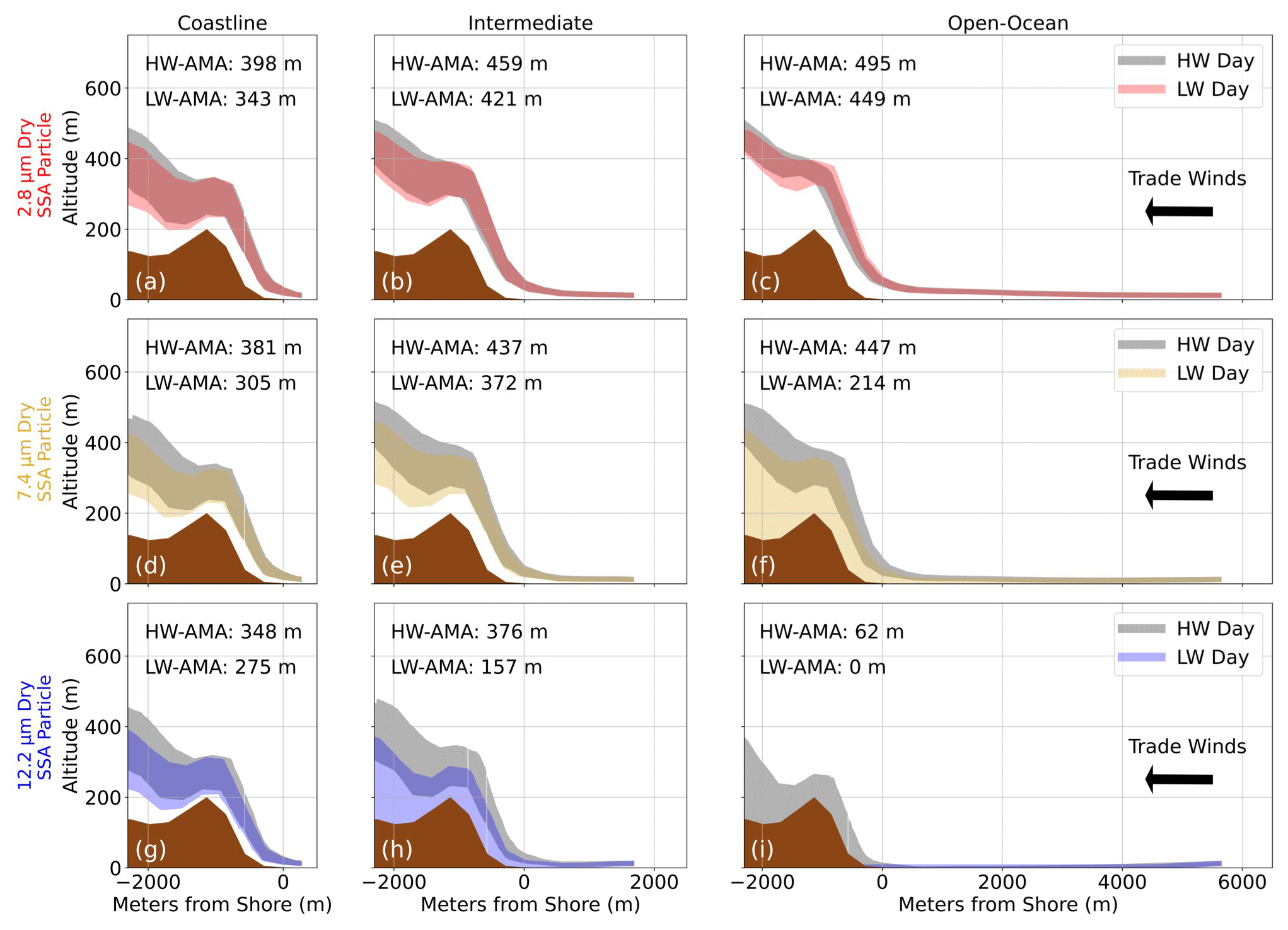
Figure 11 Cross sections from Fig. 3 were utilized to show the total trajectory ranges for both the high- and low-wind days across the three production locations. Three differently sized GSSPs were released at three production locations within these cross sections. Trajectory ranges for r_d2.8 are shown in panels (a), (b), and (c), trajectory ranges for r_d7.4 in panels (d), (e), and (f), and trajectory ranges for r_d12.2 in panels (g), (h), and (i). The color-shaded regions show trajectory ranges for the low-wind day (LW), while all the grey regions show trajectory ranges for the high-wind day (HW) for each particle size. The HW and LW average maximum altitude (AMA) are given for each plot, and the trade wind direction is generally represented as right to left in these plots, approximately perpendicular to the mountain range.

7 Discussions and implications

7.1 Important considerations for environmental variables

7.1.1 Significant wave heights vs. wind speeds

In this coastal study, H_s has a stronger correlation with SSA-SD shape parameters than U₁₀. There does appear to be a strong correlation between U₁₀ and H_s (Pearson's r=0.85) for our samples, which could imply that U₁₀ is still a viable proxy to represent coastal SSA production. Further investigation into this relationship, however, shows that the correlation between U₁₀ and H_s across an extended climatology is only Pearson’s r=0.55 for this area, and therefore the correlation we observe between these two environmental variables is artificially high. The strong correlation in our study is likely because we require onshore trade winds to sample and are more likely to observe days with trade wind swells. In the context of historical coastal SSA studies, sampling restrictions may also have resulted in an artificially strong correlation of SSA-SDs with U₁₀. Therefore, it is possible that utilizing U₁₀ in a coastal production equation for this region may misrepresent the actual production.

Once the co-relationship between H_s and U₁₀ is removed, partial correlations confirm that H_s is the only significant variable for setting coastal SSA-SD shape parameters. Utilizing H_s not only makes sense from a hydrodynamical perspective (Chomka and Petelski, 1997), but also has the potential to reduce error in production estimates created by anomalous wind estimates. In the analysis by Grythe et al. (2014), many open-ocean SSA production equations had an excessive generation of spume droplets due to anomalously high U₁₀ events, biasing global production estimates to be larger than observations. H_s often has smaller standard deviations (σ) than U₁₀. Replacing U₁₀ with H_s as the primary variable for coastal SSA production may minimize the sensitivity of the production equation. It should be noted, however, that U₁₀ should not be completely removed from coastal SSA equations, as it is essential for spume droplet production when U₁₀>9 m s⁻¹ (De Leeuw et al., 2000).

7.1.2 Considerations for sea surface temperature

Another environmental variable that was analyzed but not previously discussed is SST. Typically one would expect increasing SSA production with increasing SST, as found in Anguelova and Webster (2006) and Jaeglé et al. (2011). Correlations between SST and SSA-SDs in this study, however, show the opposite. A moderately negative correlation was found between the SSA-SDs and SST, but we hypothesize that this was due to our specific sampling environment and the wave behavior experienced in Hawai`i. There is a strong seasonality of both SST and H<sub>s</sub> in Hawai`i. During the boreal winter, the North Pacific Ocean generates large waves during strong Aleutian Lows that propagate southwards towards the Hawaiian islands. As a result, the northern shores experience peak H_s values when SSTs are lowest in Hawai`i. In the boreal summer, storms in the South Pacific generate waves that travel northwards towards the islands, meaning large waves reach the southern shores when SSTs are highest. This study took place on an eastern coastline across a period of 1 year, meaning our largest H<sub>s</sub> values came during the boreal winter when Hawai`i experiences the lowest SST. While our observed range of SST is relatively small (approximately 3.5 ^∘C), we anticipate that H_s will play a much larger role in SSA-SD variability than SST at this location.

7.2 Considerations for future observations of coastal SSA

7.2.1 The significance of the aerosol size distributions

Gathering in situ observations of SSA-SDs is notoriously difficult. Sampling limitations are imposed by the size and weight of aerosol particle sizers, accessibility to aircraft, and instrumentation costs, resulting in reduced sampling locations and frequency. Additionally, many studies characterize SSA changes based on the total mass or concentration rather than changes in size distributions due to the nature of these aerosol samplers. The lack of complete SSA-SDs has resulted in the implementation of dynamic modeling approximations (Porter and Clarke, 1997; Blanchard et al., 1984) in which SSA-SDs are assigned based on concentrations alone, independent of the environmental conditions.

Section 4 demonstrates how SSA-SD shape parameters can vary across different H_s and U₁₀ and, therefore, assigning distribution shapes blindly may be unphysical (Reid et al., 2001). Section 5 shows how SSA-SD shapes change between the open ocean and coastline, implying that open-ocean SSA-SDs may not be suitable for application to coastal observations. Lastly, Sect. 6 shows how different altitudes can have different sources of SSPs. Upper altitudes are more likely to see higher concentrations of smaller-sized GSSPs from the Open Ocean, Intermediate, and Coastline regions, while lower-altitude samples are more likely to contain ultragiant SSPs from these regions. Despite GSSPs existing in such small concentrations, they can drastically skew an SSA-SD shape depending on the sampling altitudes and the sources and sizes of SSPs present. For these reasons, observing SSA-SDs is important.

7.2.2 Observations of giant sea salt particles

A unique aspect of our sampling methodology is the ability to observe GSSPs. Because these GSSPs exist in smaller concentrations than submicron SSPs, larger sampling volumes are necessary to observe them. Additionally, their size and inertia mean aerosol inlets experience larger rates of particle loss for GSSPs, making samplers with inlets inadequate for studying these larger size ranges. Table 2 from Grythe et al. (2014) shows that only 3 of the 22 analyzed source functions account for ultragiant SSPs, and half of the equations only account for r_d>5 µm, while coastal samples from this study's Table 3 only have two studies that can observe r_d>5 µm.

Despite GSSP concentrations being much smaller than submicron SSP concentrations, they remain significant in terms of their particle mass and energy transfers as well as their potential to act as raindrop embryos and giant cloud condensation nuclei in clouds (Lasher-trapp et al., 2005; Cooper et al., 2013; Jensen and Nugent, 2017). Observing a complete range of particle sizes within a size distribution may prove vital to bettering estimates of global SSA mass and volume. We hope that the affordability and accessibility of the mini-GNI instrument may encourage future studies to consider sampling GSSPs in addition to their original SSP size range.

7.2.3 Accounting for local dynamical controls

Few studies have observed changes to SSA-SDs along the coastline and, when available, most observations occur within the lowest 20 m of the atmosphere (Table 3). SSA plume heights are highly variable and depend on local conditions such as coastal wave energetics (Chomka and Petelski, 1997) and wind speeds (De Leeuw et al., 2000). Additionally, the resulting SSPs can experience rapid vertical mixing from their production location by coastal thermals (Porter et al., 2003) and orographic lifting. If the in situ sampling method is altitude-restricted, these studies may not observe the full production potential within this location and may be more likely to see specific SSP sizes based on the conclusions in Sect. 6. GSSPs and ultragiant SSPs are more likely to experience fallout when they are produced at great distances from the coast, generating steeper gradients for these particles with altitude. Smaller GSSPs and submicron SSPs may remain aloft longer, meaning observations in coastal environments may be unfairly attributing the increase in smaller SSP concentrations to coastal production if they do not consider the contributions from the open ocean at various altitudes.

8 Conclusions

This study establishes important precedents for coastal SSA studies in the future and highlights the significance of H_s for changes to SSA-SDs in coastal environments. We set out to answer three questions.

1. How do SSA-SDs change from the open ocean to the coastal environment?

2. Which environmental variable is most significantly correlated with changes in SSA-SDs: U₁₀ or H_s?

3. How do dynamics within our sampling location contribute to variation in the SSA-SDs across different environmental conditions and altitudes?

There are notable differences between observations of SSA over the open ocean and the coastline. SSA-SDs change in cumulative concentration as well as distribution shape between these regions, indicating there may be more complicated processes in the coastal environment with regard to the production of GSSPs and ultragiant SSPs. For example, coastal SSA-SDs on average have gentler slopes, meaning there exist increased concentrations of ultragiant SSPs compared to the open ocean. When the COAST observations were compared to historical cumulative concentrations from Woodcock (1953), OCEAN N_cs were almost identical to W53, while the COAST N_cs were elevated across all observed wind and altitude ranges.

Analysis of environmental changes in coastal SSA-SDs shows a clear dependence on H_s. The visual correlation of SSA-SDs with H_s is stronger than U₁₀, and the partial correlations confirm the significance of H_s for SSA-SD shape parameters B and r_2.8. In this study, partial correlations also confirmed that the strong Pearson's r and Spearman's ρ between U₁₀ and the coastal SSA-SD shape parameters came from the strong correlation between U₁₀ and H_s. It is important to note, however, that the correlation between U₁₀ and H_s is stronger in this study than in nature due to restricting sampling to days with trade wind conditions. This is an important takeaway for future studies of coastal SSA-SDs, as sampling under specific environmental conditions may result in artificially high correlations.

Altitude observations and models highlighted the important roles that production distance from the coastline, U₁₀, and coastal orography play in setting SSA-SDs. For smaller GSSPs, fall velocities are negligible, meaning these particles are unaffected by their production distance from the coastline and have strong vertical mixing potential. Larger, ultragiant SSPs have significantly shorter atmospheric lifetimes, and the concentrations observed in this study are significantly limited by their production distance from the coastline. Because of this, observations of SSPs in a coastal environment for smaller GSSPs are likely to see a higher combination of open-ocean and coastally produced particles, while larger and ultragiant GSSPs are likely to have been produced much closer to the coastline.

Overall, these conclusions are important considerations in future campaigns that observe coastal SSA production. The analyses of coastal features specific to this sampling location provide significant insight into how they modify our SSA observations and set a precedent for future discussion of coastal SSA production. These results could have implications for modeling, as the coastline has been shown to produce higher concentrations of ultragiant SSPs compared to the open ocean, and orographic coastlines provide significant lift for GSSPs and ultragiant SSPs not typically seen over the open ocean.