the Creative Commons Attribution 4.0 License.
the Creative Commons Attribution 4.0 License.
 | 03 Nov 2023
Understanding offshore high-ozone events during TRACER-AQ 2021 in Houston: insights from WRF–CAMx photochemical modeling
Xueying Liu
Ehsan Soleimanian
Travis Griggs
James Flynn
Paul Walter
Mechanisms for high offshore ozone (O3) events in the Houston area have not been systematically examined due to limited O3 measurements over water. In this study, we used the datasets collected by three boats deployed in Galveston Bay and the Gulf of Mexico during the Tracking Aerosol Convection Interactions ExpeRiment – Air Quality (TRACER-AQ) field campaign period (September 2021), in combination with the Weather Research and Forecasting (WRF) coupled Comprehensive Air quality Model with Extensions (CAMx) modeling system (WRF–CAMx), to investigate the reasons for high offshore O3. The model can capture the spatiotemporal variability in the daytime (10:00–18:00 central daylight time, CDT) O3 for the three boats (R > 0.7) but tends to overestimate O3 by ∼ 10 ppb on clean days and underestimate O3 by ∼ 3 ppb during high-O3 events. The process analysis tool in CAMx identifies O3 chemistry as the major process leading to high-O3 concentrations. The region-wide increase in the long-lived volatile organic compounds (VOCs) through advection transits O3 formation to be more sensitive to NOx, leading to more O3 production under a NOx-limited regime. In addition, the VOC-limited O3 formation is also boosted along western Galveston Bay and the Gulf Coast under high-NOx conditions brought by the northeasterly winds from the Houston Ship Channel. Two case studies illustrate that high offshore O3 events can develop under both large- and mesoscale circulations, indicating both the regional and local emissions need to be stringently controlled. Wind conditions are demonstrated to be important meteorological factors in such events, so they must be well represented in photochemical models to forecast air quality over the urban coastal regions accurately.
- Article
(13890 KB) - Full-text XML
-
Supplement
(2070 KB) - BibTeX
- EndNote


The greater Houston area has been designated as ozone (O3) nonattainment by U.S. Environmental Protection Agency (EPA) under the standards of the National Ambient Air Quality Standards (NAAQS; Nonattainment Areas for Criteria Pollutants (Green Book), 2023). O3 is a secondary criteria pollutant, whose formation is nonlinearly dependent on the relative abundance of its precursors, namely volatile organic compounds (VOCs) and nitrogen oxides. Houston experiences significant anthropogenic emissions of these precursors, mainly from transportation and petrochemical facilities along the Houston Ship Channel (Leuchner and Rappenglück, 2010; Soleimanian et al., 2022). In addition, due to its unique location at the land–water interface, high-O3 events in Houston are known to be related to complex meteorological conditions with the interactions between synoptic and mesoscale circulations. Dry and polluted continental air masses brought by northerly winds after the cold front passage are often linked with O3 exceedances (Darby, 2005; Rappenglück et al., 2008; Ngan and Byun, 2011). Extremely high O3 can occur under a land breeze–sea breeze recirculation, in which the land breeze in the morning transports the pollution-laden air toward Galveston Bay or the Gulf of Mexico, followed by the return of the aged pollutants in the afternoon by the onshore bay or sea breeze (Banta et al., 2005; Caicedo et al., 2019; Li et al., 2020). Such high-O3 events in coastal urban regions are challenging for air quality models to capture, as the physical and chemical processes of O3 over both land and water need to be well constrained (Caicedo et al., 2019; Bernier et al., 2022).
To understand the interplay among meteorology, emissions, and chemistry, various field campaigns have been deployed in the Houston area, such as the Texas Air Quality Study in 2000 and 2006 and the Deriving Information on Surface Conditions from COlumn and VERtically Resolved Observations Relevant to Air Quality (DISCOVER-AQ) in 2013. A common goal of these field campaigns was to evaluate the predictive ability of numerical weather and air quality models using the collected observations (Misenis and Zhang, 2010; Yu et al., 2012; Li and Rappenglück, 2014; Mazzuca et al., 2016; Pan et al., 2017). Although these studies greatly improve our understanding of the reasons for high-ozone events in Houston, they mainly focused on the onshore area, due to the absence of offshore measurements. Higher levels of O3 over waterbodies than the adjacent land have been observed in other coastal regions with poor air quality, such as Chesapeake Bay and Lake Michigan, due to several factors including, but not limited to, the offshore advection of polluted air masses, photochemical productions from local (e.g., marine traffic) and aged land emissions, shallow marine planetary boundary layers (PBLs), the lack of NOx titration, and low dry deposition rates (Dye et al., 1995; Goldberg et al., 2014; Sullivan et al., 2019; Abdi-Oskouei et al., 2022; Dreessen et al., 2023). Air quality modeling evaluations against these observations show difficulties in the numerical prediction of O3 over water, with an overall positive bias for low O3 and negative bias for high O3, due in part to the misrepresentation of marine meteorology and PBL (Dreessen et al., 2019; Abdi-Oskouei et al., 2020; Dacic et al., 2020; Baker et al., 2023). However, to our knowledge, high-O3 events off the Houston coast in Galveston Bay and the Gulf of Mexico have not been systematically examined. The predictive ability of photochemical models in capturing such events has yet to be quantified.
More recently, the Tracking Aerosol Convection Interactions ExpeRiment – Air Quality (TRACER-AQ) field campaign revisited the Houston area in September 2021. The campaign implemented a variety of observational platforms, covering both offshore and onshore locations, such as stationary sites, boats, lidar, ozonesondes, and airborne remote sensing. In particular, instruments on board three boats continuously collected O3 and meteorological data from July to October over Galveston Bay and the Gulf of Mexico, which provide a valuable opportunity to understand the reasons driving high-O3 concentrations over water and the O3 nonattainment at air quality monitors near the Houston coastline. Furthermore, the Texas Commission on Environmental Quality (TCEQ) has created a new emission inventory for its 2019 State Implementation Plan (SIP) modeling platform to conduct photochemical simulations using the Comprehensive Air quality Model with Extensions (CAMx) driven by the Weather Research and Forecasting (WRF) meteorology. Using the established new emissions inventory and observations, an evaluation of the offshore O3 prediction can provide insights into model deficiencies over water and help improve air quality forecasting in coastal urban regions.
This study aims to improve our understanding of high offshore O3 concentrations in the Houston coastal zone during the TRACER-AQ 2021 field campaign, based on observations and WRF–CAMx modeling, a regulatory model used by TCEQ. We first evaluate the performance of model simulations of O3 and then investigate the reasons causing high-O3 events relative to clean days, taking advantage of the process analysis tools from CAMx. Last, we present two case studies to better understand the development of elevated O3 over water. Potential sources of model bias are also discussed.
2.1 Meteorological and air quality observations
TCEQ has O3 and other pollutants routinely measured at the Continuous Ambient Monitoring Station (CAMS) across the Houston region. Some of these stations also observe meteorological variables, such as wind speed and direction, temperature, and relative humidity (RH). These data can be downloaded from the Texas Air Monitoring Information System (TAMIS, https://www17.tceq.texas.gov/tamis/index.cfm?fuseaction=home.welcome, last access: 27 October 2023) website. A commercial shrimp boat and a pontoon boat owned by the University of Houston (UH) were operated mainly on the east and west sides of Galveston Bay, respectively. Another commercial boat, the Red Eagle, was docked to the north of Galveston Island and typically traveled up to 90 km offshore in the Gulf of Mexico and occasionally northward through the Ship Channel to the port of Houston. Automated O3 sampling instruments were installed on the three boats, with a compact weather station measuring temperature, pressure, RH, and wind conditions. The sample inlet was attached to an elevated location on the boats to avoid titration from the exhausts of the boats. Details of these devices can be found in Griggs et al. (2023). In addition, ozonesondes were launched from the pontoon and Red Eagle boats on selected days and locations to investigate the vertical O3 profiles. All the campaign data can be found on the TRACER-AQ website (https://www-air.larc.nasa.gov/cgi-bin/ArcView/traceraq.2021, last access: 27 October 2023).
During the offshore operational period of July to October, hourly averaged O3 mixing ratios exceeded 100 ppb several times. We identified O3 exceedance days, when offshore boat O3 observations registered a daily maximum 8 h average (MDA8) O3 in exceedance of 70 ppb, which is the current criterion of the NAAQS for O3. Six episodes with high O3 were obtained for 26–28 July, 25 August, 6–11 September, 17–19 September, 23–26 September, and 6–9 October. These episodes are accompanied by at least one CAMS site exceeding the 70 ppb MDA8 O3 threshold, indicating an extensive land–water air mass interaction.
2.2 WRF and CAMx model configuration
This study used the WRF model v3.9.1.1. We set up three domains with different horizontal resolutions that cover the contiguous United States, southeastern Texas, and the Houston–Galveston–Brazoria region and referred to as domains d01, d02, and d03, respectively, as shown in Fig. 1. The corresponding horizontal resolutions and grid numbers for d01–d03 are 12 km × 12 km (373 × 310 grids), 4 km × 4 km (190 × 133 grids), and 1.33 km × 1.33 km (172 × 184 grids), respectively. All domains have identical vertical resolutions, with 50 hybrid sigma–eta vertical levels spanning from the surface to 10 hPa. Boundary conditions of the two inner domains were generated from the outer domain.
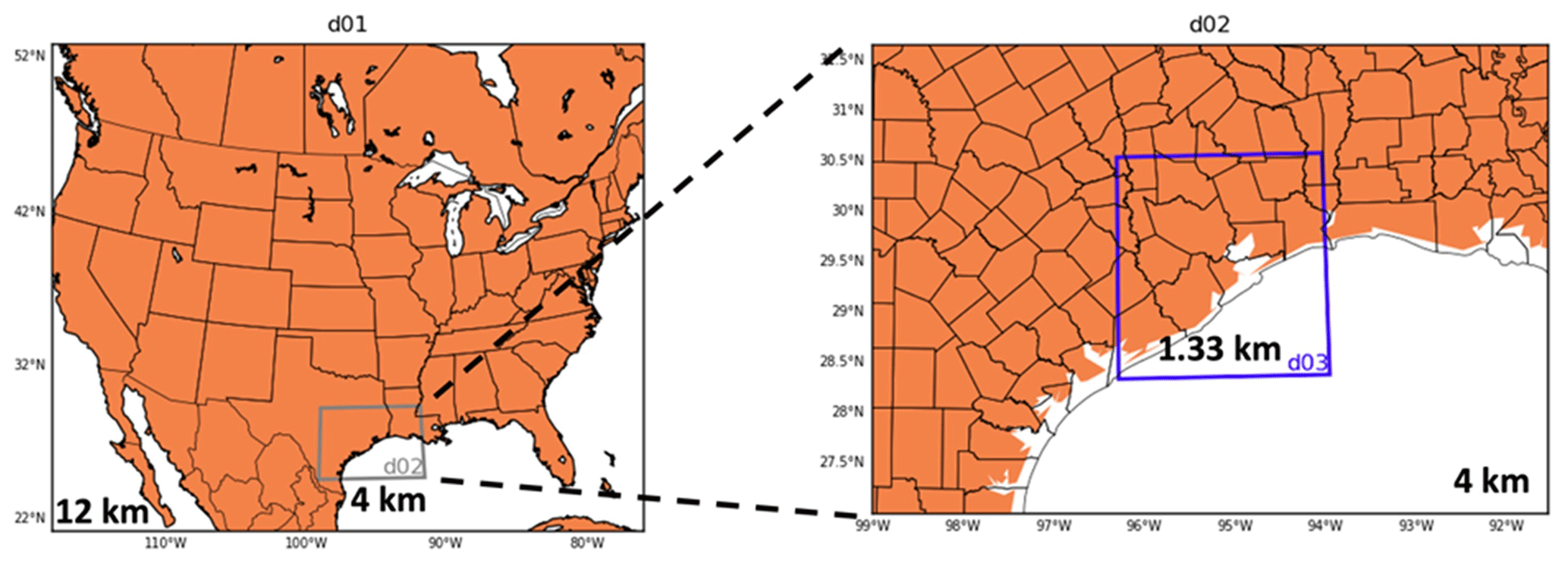
Figure 1WRF nested modeling domains and horizontal resolutions.
To select the WRF configurations that best represent the monitoring data, we designed eight model experiments with different initial and boundary condition (IC/BC) inputs, microphysics options, PBL schemes, data assimilation methods (e.g., observation nudging), and reinitializing techniques. Details of the design and evaluation of each experiment can be found in Liu et al. (2023). Based on the campaign-wide evaluation of the modeled meteorology, the best simulation was used to drive the CAMx model. The model configuration of the best simulation includes the hourly High-Resolution Rapid Refresh (HRRR) meteorological data as IC/BC inputs, the local closure Mellor–Yamada–Nakanishi–Niino (MYNN) PBL option (Nakanishi and Niino, 2009), and the Morrison double-moment (2M) microphysics scheme (Morrison et al., 2009), with no nudging and reinitializing techniques applied. Other settings used for the WRF simulation include the Monin–Obukhov similarity surface layer (Foken, 2006), the Noah land surface scheme (Chen and Dudhia, 2001), the rapid radiative transfer model (RRTM) longwave and shortwave radiation schemes (Iacono et al., 2008), and the new Tiedtke cumulus parameterization (Zhang et al., 2011).
This study also used the CAMx model v7.10. The three CAMx domains aligned with the WRF grids but had smaller spatial coverage. The corresponding horizontal resolutions and grid numbers for domains 1–3 are 12 km × 12 km (372 × 244 grids), 4 km × 4 km (156 × 126 grids), and 1.33 km × 1.33 km (153 × 162 grids), respectively. All domains have identical vertical resolutions, with 30 vertical levels from the surface to ∼ 100 hPa. The IC/BC inputs for the outmost domain are from the GEOS-Chem (v12.2.1) global simulation, with the National Emissions Inventory (NEI) 2011 nitrogen oxide (NOx) emissions scaled down to 2021. The Carbon Bond version 6 revision 5 (CB6r5) was used for gas-phase chemistry, including the inorganic iodine depletion of O3 over oceanic water (Burkholder et al., 2019). The first-order eddy viscosity (K-theory) diffusion scheme was selected for vertical mixing within the PBL, in which the vertical diffusion coefficients (Kv) were supplied from WRF outputs. Dry deposition is based on the Wesely scheme (Wesely, 1989).
Emission files with 12 and 4 km spatial resolutions from the preliminary 2019 SIP modeling platform provided by TCEQ are used in the simulation. These emissions include anthropogenic emissions, biogenic emissions generated from the Biogenic Emission Inventory System (BEIS), wildfire emissions based on the Fire INventory from NCAR (FINNv2), and ship emissions estimated from the Gulfwide Emissions Inventory (GWEI). No lighting emissions are included in the model. Since our domains are smaller than those in the SIP modeling, the original emission files were cropped to match the grid boundaries for CAMx to read properly. In addition, we redistributed the on-road emissions from 4 to 1.33 km over the Houston area. The 4 km emission fluxes were first disaggregated evenly to the 1.33 km grids and then collected onto major roads, using a 1 km rasterized road shapefile to produce on-major-road 1.33 km emissions. Some 1.33 km grid points off the major roads had missing values, which were filled using a smoothing method that averaged eight nearby grid points. The scaling factors for on- and off-major-road emissions were kept in order to maintain the on-road emission budget consistent before and after the spatial redistribution. Finally, total emissions were calculated by adding the 1.33 km on- and off-major-road emissions. The emissions for other sectors were also similarly interpolated to 1.33 km, without separating into no- or off-major-road temporary emissions. The redistributed emissions were tested to perform better in capturing the on-road distributions than using the Flexi-nesting function in CAMx (Fig. S1 and Table S1 in the Supplement), which can regrid the emissions on the fly.
The simulation was performed for two periods, 20–30 July and 20 August–13 October, to cover the six high-O3 episodes defined in Sect. 2.1. A 10 d spin-up before each period was applied. Other days in the two periods are considered clean scenarios, with low-O3 concentrations. Process analysis, including integrated process rate analysis (IPR), integrated reaction rate analysis (IRR), and chemical process analysis (CPA), was turned on when running the model. IPR contains O3 change rate from several chemical and physical processes, such as chemistry (CHEM), horizontal and vertical advection (ADV) and diffusion (DIF), and deposition (DEP). IRR provides detailed information about the reaction rate of all the chemical reactions in the CB6r5 scheme. CPA improves upon IRR by computing parameters useful for understanding O3 chemistry, such as the O3 production rate and regime. The abundance and reactivity of ozone precursors determine the ozone production regime, which can be indicated by the loss of HOx radicals (HOx = OH + HO2) through the termination of ozone chain reactions. Under low-NOx conditions, the most important HOx loss is the self-reaction of the hydroperoxyl radical (HO2), producing hydrogen peroxide (H2O2), which is used to represent NOx-limited ozone production. In urban areas with high-NOx concentrations, the dominant sink for HOx radicals is the oxidation of nitrogen dioxide (NO2) by hydroxyl radical (OH), resulting in the production of nitric acid (HNO3). Thus, the O3 formation regime in the model is determined based on the ratio of H2O2 production rate from HO2 self-reaction to HNO3 production rate from OH reaction with NO2, in which < 0.35 indicates a VOC-limited regime, and ≥ 0.35 indicates a NOx-limited regime (Sillman, 1995). There is no transition scheme available in this method.
3.1 Evaluation of O3 simulations
The time series of the daytime (10:00–18:00 central daylight time, CDT) mean O3 at the three boats are shown in Fig. 2a, and the evaluation statistics are listed in Table 1. The evaluation excludes nighttime data to reduce the effects from land, as the boats stayed at the dock at night. Indeed, an hourly time series evaluation with nighttime data included (Fig. S2 and Table S2 in the Supplement) shows a larger bias between modeled ozone and boat observations. The spatiotemporal variability in the daytime O3 at the three boats is well captured by the model, with a correlation coefficient (R) value greater than 0.70. Overall, the model overestimates daytime O3 by 4.57 ppb (11 %), 7.82 ppb (22 %), and 4.35 ppb (9 %) for the pontoon boat, Red Eagle, and shrimp boat, respectively. On episode days, high-O3 mixing ratios can be found over Galveston Bay and the Gulf of Mexico (Fig. 2b). The model captures some of the variability (R = 0.42–0.51), with negative mean bias (MB) values of ∼ 4.5 ppb (8 %) for the pontoon and shrimp boats and a nearly unbiased simulation (MB = 0.05 ppb) for the Red Eagle boat. While the O3 variability is better predicted on clean days (R = 0.69–0.76), the model shows higher values of MB than those on high-O3 days, ranging from 9.15 ppb (29 %) to 11.28 ppb (41 %), which drives the overall model overestimation.
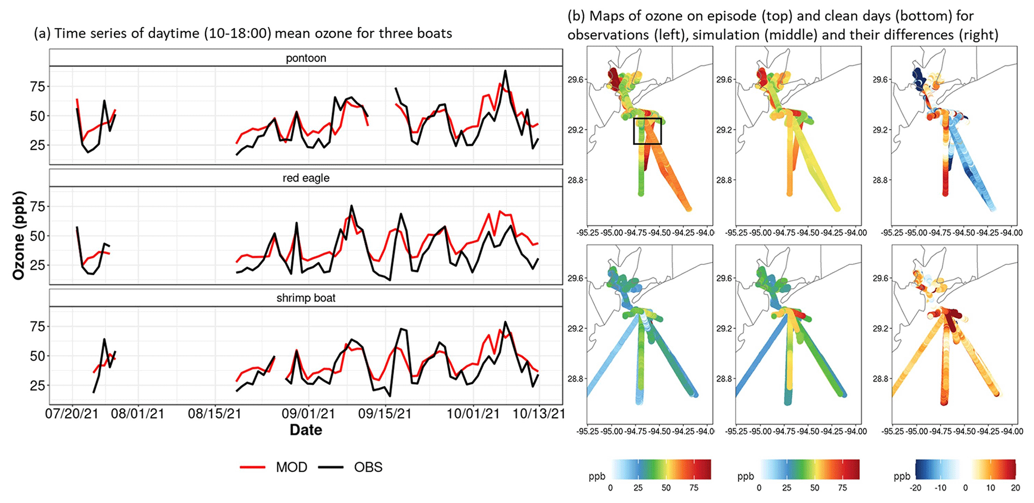
Figure 2(a) Time series of daytime (10:00–18:00 CDT) mean ozone for observations at three boats (black) and simulations (red). (b) Maps of observed (left column), simulated (middle column), and the difference in (right column) ozone during ozone episodes (top row) and clean days (bottom row). The black box shows the selected offshore region for process analysis in the next section.
Table 1Daytime (10:00–18:00 CDT) ozone evaluation metrics at three boats, including the observed and simulated mean values, correlation coefficient (R), mean bias (MB), normalized mean bias (NMB), mean absolute error (MAE), and root mean square error (RMSE).
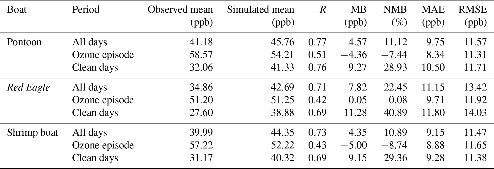
Table 2Daytime (10:00–18:00 CDT) ozone evaluation metrics at CAMS sites. The metrics are the same as in Table 1.
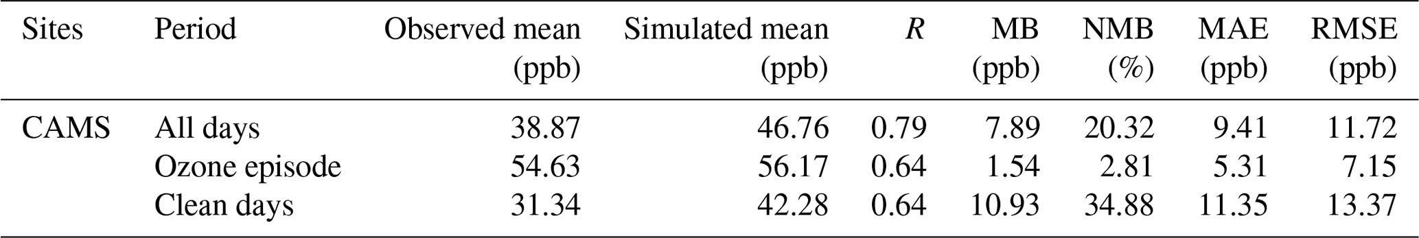
While we did not find any previous efforts modeling offshore O3 in the Houston area to compare our results, an evaluation against onshore measurements can help validate our model performance. The time series of the daytime mean O3 from simulations and observations from CAMS sites are displayed in Fig. 3, and the evaluation statistics are summarized in Table 2. The model captures the onshore O3 variability (R = 0.79), with an overall overestimation of 7.89 ppb (20 %), mainly due to the high positive bias of 10.93 ppb (34 %) on clean days. This result is comparable with the model performance from previous studies focusing on the same area (e.g., Xiao et al., 2010; Pan et al., 2015; Kommalapati et al., 2016), which further verifies the reliability of our model settings.
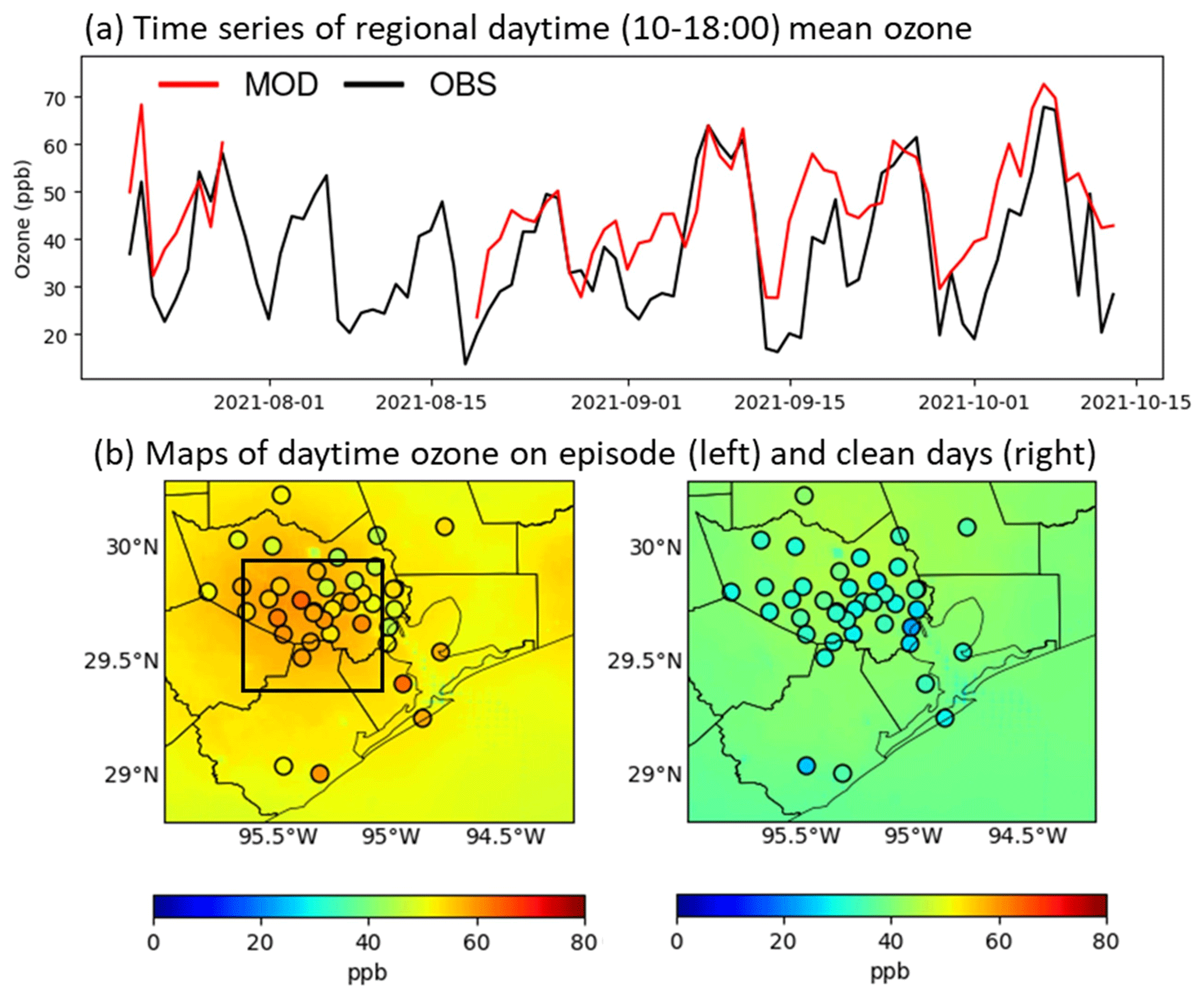
Figure 3(a) Time series of daytime (10:00–18:00 CDT) mean ozone for observations at CAMS sites (OBS; black line) and simulations (MOD; red line). (b) Maps of observed (points) and simulated (background) daytime ozone during ozone episodes (left) and clean days. The black box shows the selected onshore region for process analysis in the next section.
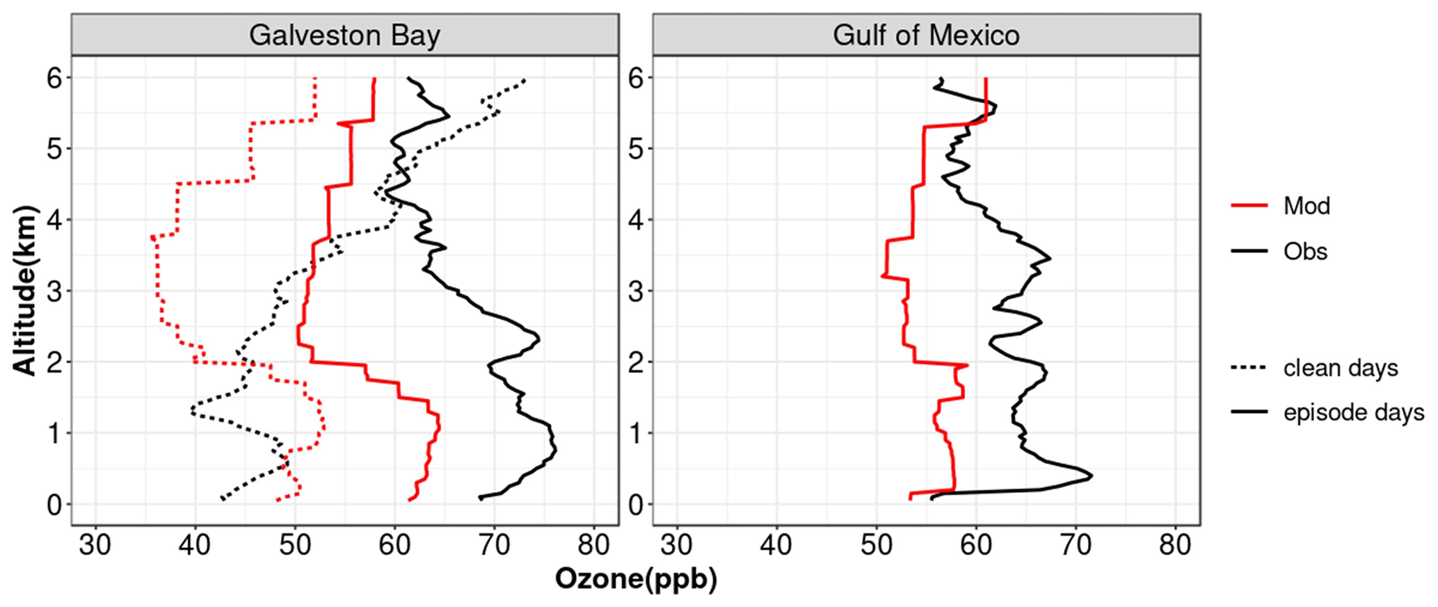
Figure 4Ozone vertical distribution from the afternoon (12:00–18:00 CDT) ozonesonde launches (Obs; black lines) and simulations (Mod; red lines) at Galveston Bay, averaged on clean days (dashed lines) and ozone episode days (solid lines). The Gulf of Mexico only sampled ozone on high-ozone days.
We also evaluated the modeled vertical O3 profiles against the afternoon (12:00–18:00 CDT) ozonesondes launched over Galveston Bay and the Gulf of Mexico. During the study period, there were five and nine afternoon launches over Galveston Bay on clean and O3 episode days, respectively, while the Gulf of Mexico only had five afternoon launches during high-O3 events. All the ozonesondes available for high-O3 conditions are from the two episodes of 6–11 and 23–26 September. The average O3 profiles from these launches are shown in Fig. 4. Free-tropospheric O3 with altitudes greater than 2 km is underestimated for both locations on both clean and O3 episode days, which indicates that the long-range transported O3 is underrepresented by the model. Over Galveston Bay, the overestimation of O3 within the mixed layer below 2 km on clean days changes to underestimation on episode days, and the underestimation increases from 5 ppb at the surface to 10 ppb near 1 km. The two high-O3 episodes in September are featured by a O3 plume between 2–3 km, as shown by the O3 lidar observations in Liu et al. (2023), which is missed by the model, as shown by the two example days on 9 and 24 September of each episode over Galveston Bay (Fig. S3 in the Supplement). The underestimation of O3 in the lower free troposphere and the mixed layer on episode days can be partly explained by the missing of the high-O3 plumes, which can be mixed down when the cap inversion is weak (Liu et al., 2023). There is an approximately 10 ppb underestimation across all altitudes below 4 km over the Gulf of Mexico. An ozonesonde from the Gulf of Mexico on 9 September recorded high ozone up to the top of the marine layer at 370 m, which is missed by the model and leads to the highest bias. This case will be discussed in the case study in Sect. 3.3.
To conclude, despite the overall model bias for vertical O3 distributions, the acceptable model performance for offshore and onshore O3 prediction at the surface indicates that the modeling system can be applied to conduct process analysis and help identify the processes influencing high-O3 concentrations over the water surface.
3.2 Process analysis over the Gulf of Mexico
This section examines how the CAMx-simulated O3 processes change during high-O3 episodes relative to clean days. The process analysis is calculated over a subregion of the Gulf of Mexico, with high-O3 mixing ratios observed (black box in Fig. 2b) and integrated across the lowest five model layers that are comparable to the morning PBL heights over water. The diurnal average of each process on clean and O3 episode days is shown in Fig. 5a. Chemistry (CHEM) is the major O3 source during daytime and becomes the primary O3 sink after sunset. Advection (ADV) serves as a pathway for an O3 sink for most hours, especially during the day, while vertical diffusion (DIF) mostly contributes as an O3 source. Deposition (DEP) constantly removes O3 from the atmosphere at all hours, yet with a marginal value of 0.1 ppb h−1. Similar patterns can be found over the Houston urban area, with a much bigger magnitude (Fig. S4 in the Supplement). During high-O3 events, CHEM is the most important process causing higher-O3 levels over water relative to clean days, followed by vertical DIF (Fig. 5b). We examined the simulated O3 vertical profiles and PBL heights averaged over the process analysis region on clean and episode days in Fig. S5 in the Supplement. O3 across the entire profile is higher on episode days than clean days, indicating an elevated O3 background on high-O3 days. In addition, the profiles of potential temperature observed by the ozonesondes show an inversion layer at ∼ 1.5 km on episode days (Fig. S6 in the Supplement). More vertical diffusion can occur if high O3 in the inversion layer is mixed down from above the PBL when the capping inversion is weak (Liu et al., 2023).
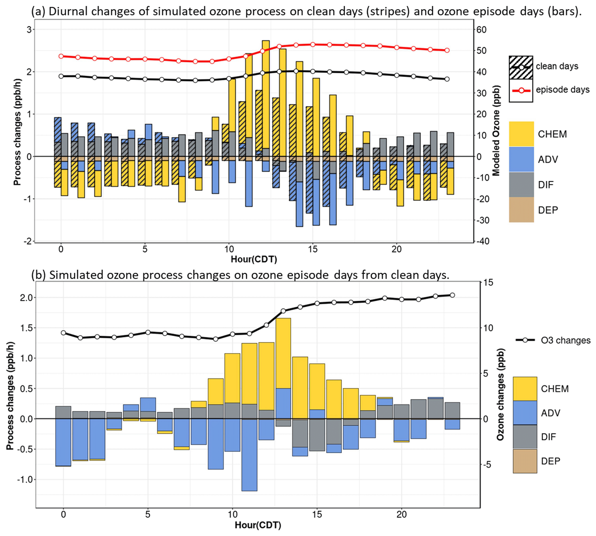
Figure 5(a) Diurnal changes in the simulated ozone processes over the Gulf of Mexico (black box in Fig. 2), including chemistry (CHEM), advection (ADV), vertical diffusion (DIF), and deposition (DEP) on clean days (stripes) and O3 episode days (bars) integrated across the lowest five model layers. Overlaid lines and points are simulated hourly ozone on clean (black) and O3 episode (red) days. (b) Process (filled bars) and O3 (black line) changes during high-O3 episodes relative to clean days.
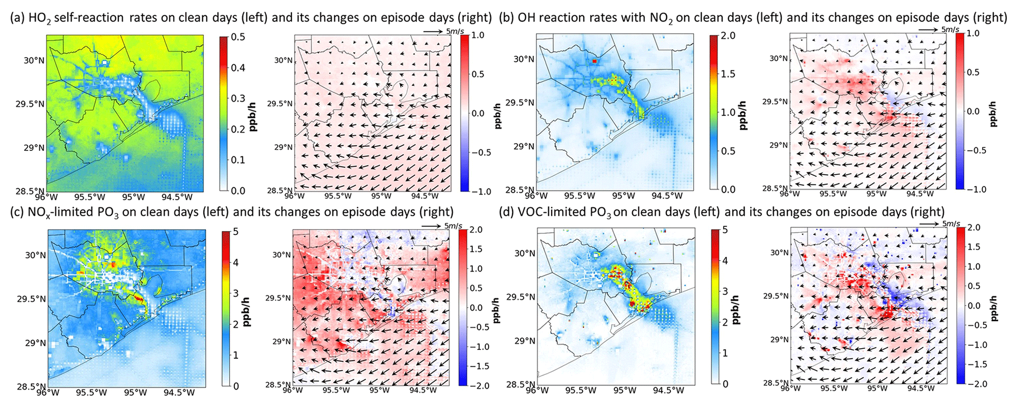
Figure 6Maps of the rate (ppb h−1) of HO2 self-reaction (a), OH reaction with NO2 (b), ozone production (PO3) under NOx-limited (c) and VOC-limited (d) regimes on clean days (left), and its changes under episode days (right) during midday (11:00–15:00 CDT). Black arrows indicate the simulated wind speed and directions averaged on high-O3 days.
The CPA analysis can provide more insights into the enhanced O3 production during high-O3 events. We first investigated the rates of HO2 self-reaction and OH reaction with NO2 in Fig. 6a and b, since they are used by the model to determine the O3 chemical regime. A region-wide increase in the HO2 self-reaction rate leads to the enhancement of PO3 under a NOx-limited regime (Fig. 6c). Similarly, the frequency of PO3 under a NOx-limited regime also increases regionally (Fig. S7 in the Supplement). The frequency at each grid cell is the ratio of the number of hours with a greater than zero NOx-limited PO3 to the total midday hours (11:00–15:00 CDT) during the study period. HO2 is formed, following the oxidation of VOCs by OH. Thus, we further compared the OH reactivity of VOCs averaged from 11:00 to 15:00 CDT on clean and episode days in Fig. 7. Isoprene has the highest contribution to the total VOC reactivity on the land, but its reactivity does not increase during high-O3 events. Instead, paraffin, formaldehyde, and acetaldehyde are the three VOCs experiencing the highest increase in the reaction rate with OH over both land, by 0.22 ppb h−1 (84 %), 0.19 ppb h−1 (45 %) and 0.15 ppb h−1 (73 %), and water, by 0.18 ppb h−1 (114 %), 0.15 ppb h−1 (44 %) and 0.11 ppb h−1 (82 %), respectively, which indicates a higher contribution from regional transport on episode days, as they are relatively long-lived VOCs capable of traveling long distances. Indeed, the paraffin IPR analysis shows that the ADV process dominates the increase in the paraffin during morning hours from 06:00 to 11:00 CDT over water (Fig. S8 in the Supplement). The trajectory analysis focusing on two O3 episodes in September shows that air masses were transported from the northern/central states (Soleimanian et al., 2023), consistent with the wind directions demonstrated in Fig. 6. Such wind conditions can also bring NOx emissions from the Houston Ship Channel downwind towards the western side of Galveston Bay and the Gulf of Mexico, causing a higher-OH reaction rate with NO2 (Fig. 6b) and enhanced PO3 under a VOC-limited regime (Fig. 6d) therein.
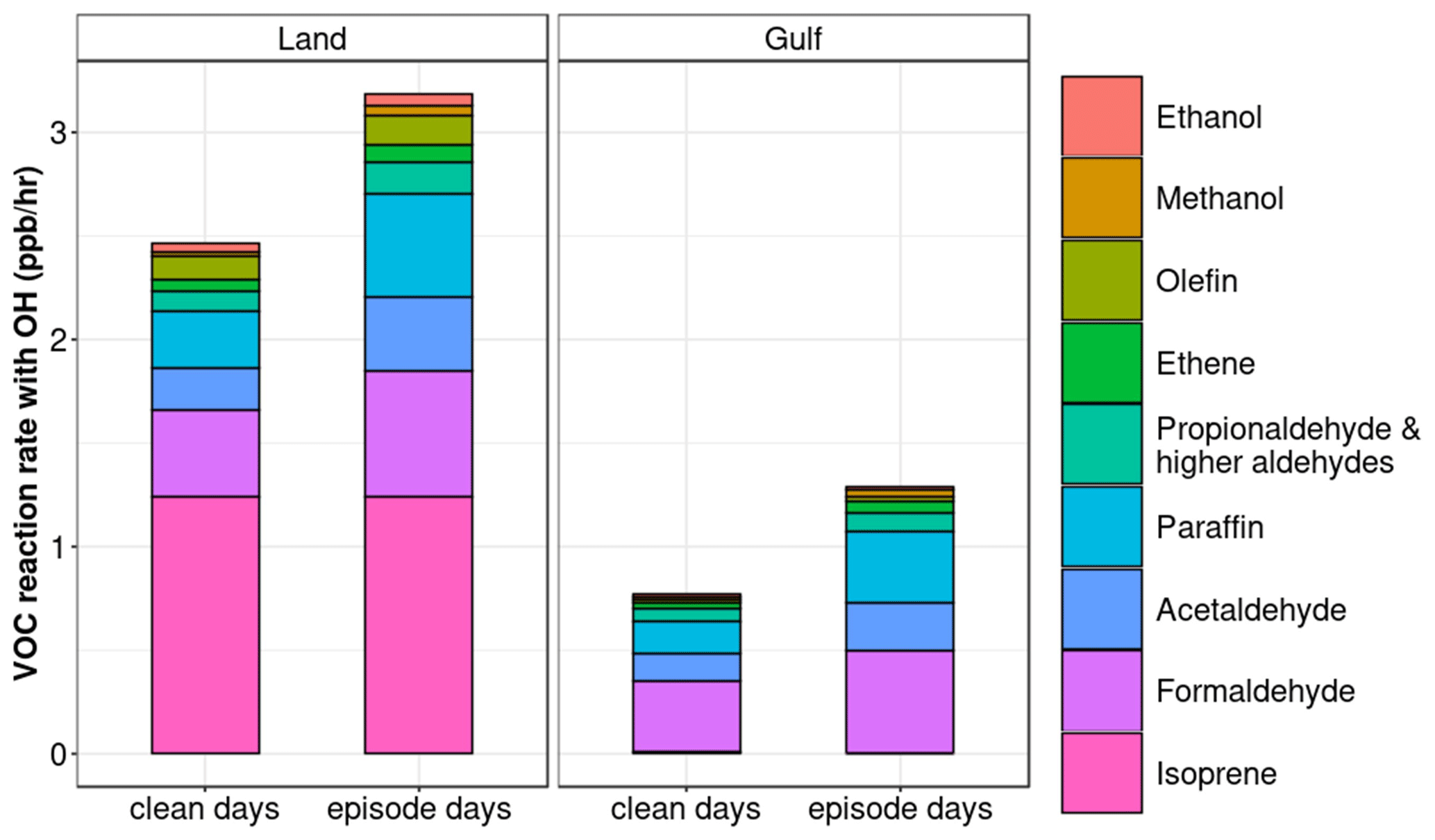
Figure 7OH reaction rates with different VOCs on clean days and ozone episode days during 11:00–15:00 CDT over the urban area (Land; black box in Fig. 3) and the Gulf of Mexico (Gulf; black box in Fig. 2).
In summary, O3 chemistry is the major process responsible for the high-O3 mixing ratios over the Gulf of Mexico during the study period. The VOC species with a long lifetime advected from the northeastern increase over land and water, leading to a region-wide enhancement of PO3 under a NOx-limited regime. The downwind transport of NOx from the Houston Ship Channel also expands the VOC-limited area towards the west side of Galveston Bay and the Gulf of Mexico, contributing to the higher-than-normal PO3.
3.3 Case studies
Although the above analysis reveals the general reasons responsible for the high offshore O3 events, the multiple-day average can miss out on some important aspects regarding the causes of these events. In this section, we selected 2 case days, 9 September and 7 October, to further demonstrate the development process of high O3 in detail.
3.3.1 Case study of 9 September 2021
Multiple CAMS sites exceeded the 70 ppb MDA8 O3 standard on 9 September, with the Red Eagle boat sampling the up to 115 ppb per 1 min O3 in the Gulf of Mexico off the coast of Galveston Island. The hourly progression of the observed and simulated O3 is displayed in Fig. 8 and overlaid with modeled winds. In the morning, the study area was dominated by northerly winds bringing the fresh emissions offshore, while the pontoon boat was sampling over the west side of Galveston Bay, and the Red Eagle boat was traveling in the Gulf of Mexico off the coast of Galveston Island. The ozonesonde launched near 09:00 CDT shows a moderate level of O3 (∼ 55 ppb) below the shallow marine boundary layer of 200 m overlaid by a residual layer with a maximum O3 mixing ratio of 63 ppb at ∼ 500 m (Fig. 9a). Around 11:00–12:00 CDT, with high solar radiation, the seaward-transported emissions formed O3 through photochemical reactions over water, which were captured by the Red Eagle boat with an hourly peak O3 mixing ratio of 92 ppb (Fig. 10a). Correspondingly, the O3 vertical profile from the 11:45 CDT balloon launch at the Red Eagle deck recorded the highest O3 of 110 ppb at ∼ 315 m (Fig. 9b).
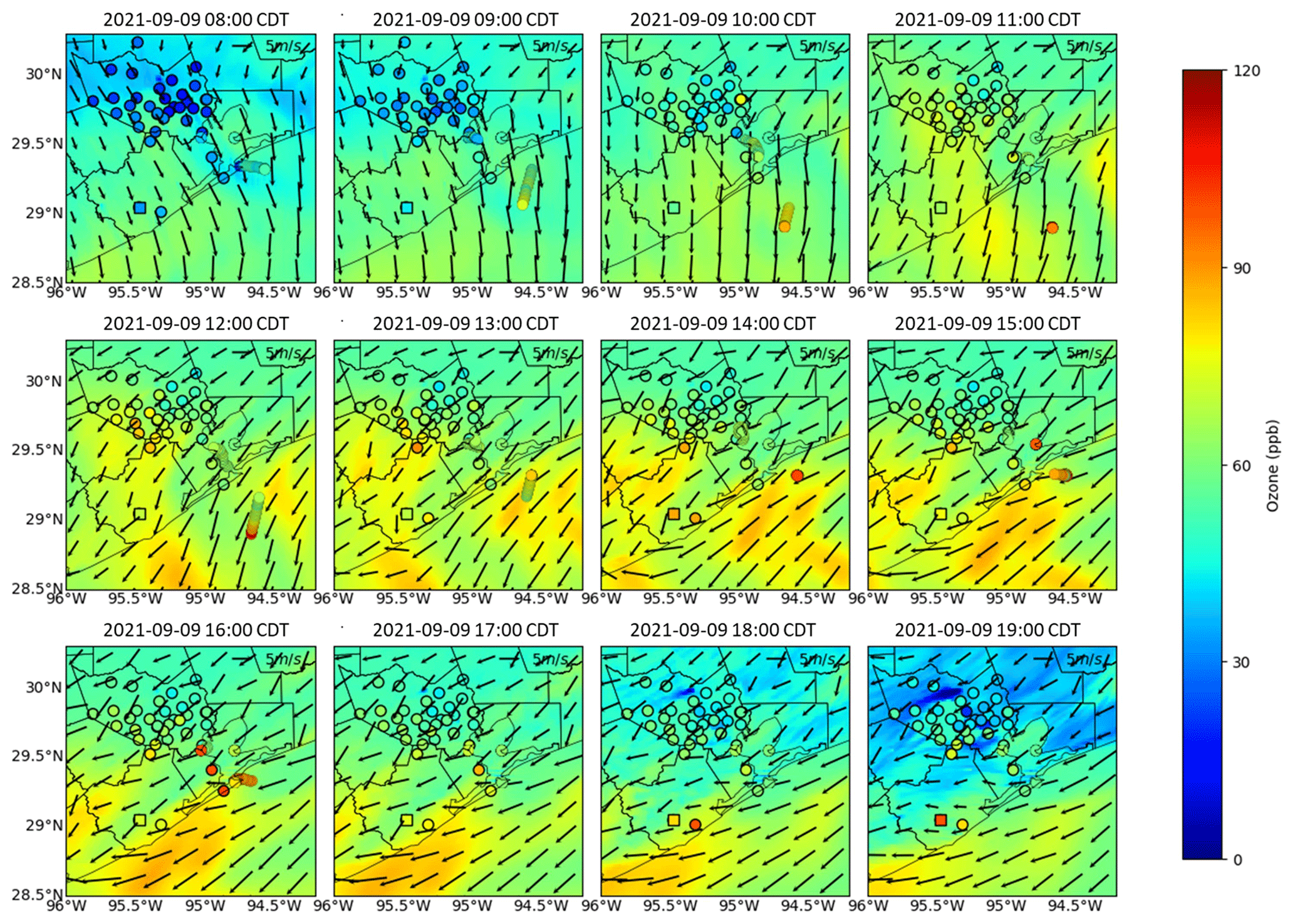
Figure 8Hourly simulated ozone distributions (color contours) from 08:00 to 19:00 CDT on 9 September overlaid with winds (arrows). Onshore and offshore dots indicate ozone from CAMS sites and boat observations. The squares highlight the Lake Jackson CAMS site.
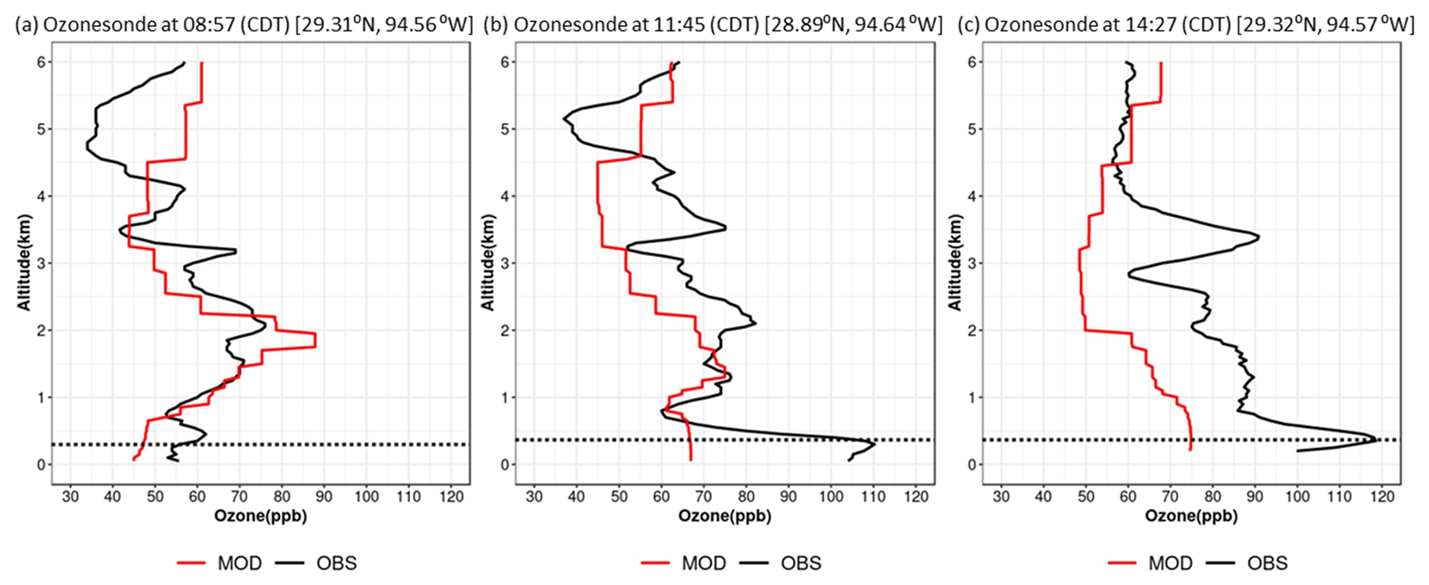
Figure 9Ozone vertical profiles from ozonesondes (black line) and model simulations (red line) at 08:57 (a), 11:45 (b), and 14:27 CDT (c) on 9 September. Dashed black lines indicate the observed boundary layer height.
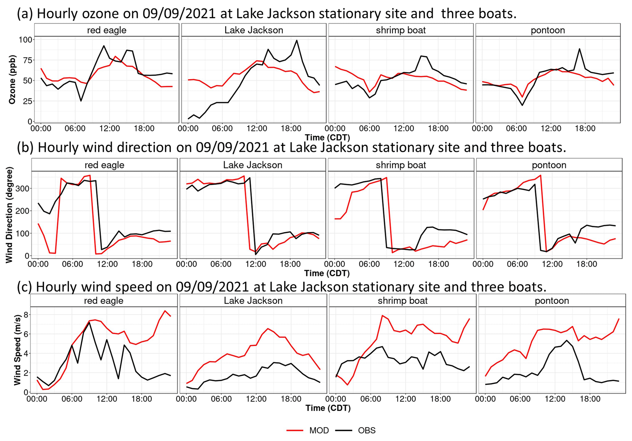
Figure 10Hourly ozone (a), wind direction (b), and wind speed (c) on 9 September from observations at the Lake Jackson CAMS site (squares in Fig. 8) and three boats (black) in comparison with the model simulations (red).
However, the model missed these peak values because the simulated wind speed is up to 4 m s−1 higher than observations (Fig. 10c), making the plume advect faster. This also leads to a 2 h earlier arrival of the modeled O3 peak at the Lake Jackson coastal site (squares in Fig. 8) than the observed first peak at 14:00 CDT (Fig. 10a). At the same time, another plume was brought into the Gulf of Mexico from the eastern boundary of the domain as the wind directions changed from north to east. As the Red Eagle boat steered back to Galveston Island, all three boats sampled this plume at 14:00–17:00 CDT, resulting in the second O3 peak at the Red Eagle boat and the only O3 peak at the other two boats. The ozonesonde launched at 14:27 CDT from the Red Eagle boat (Fig. 9c) observed O3 reaching 118 ppb in the plume at ∼ 370 m. This plume was continuously transported southwestward and reached the Lake Jackson site at 19:00 CDT, producing a second O3 peak. Due to the overestimated wind speed and the simulated wind direction not completely veering to the east as in the observations (about 100∘ in Fig. 10b), the model failed to predict the timing and the magnitude of the O3 peaks caused by the second plume. The process analysis on this day over the Gulf of Mexico (black box in Fig. 2) shows that ADV, in addition to CHEM, contributes to the enhanced O3 levels at 10:00 and 13:00 CDT (Fig. S9 in the Supplement), which, respectively, corresponds to the two plumes under northerly and easterly winds and highlights the importance of regional transport. This also demonstrates that the contributions from ADV to the increase in the O3 can be high on some specific cases, which can be averaged out in our composite analysis of Fig. 5.
In summary, the wind direction changes from the north to the east on 9 September caused two O3 peaks, as captured by the Red Eagle boat and the Lake Jackson site. This corresponds to the two simulated ozone plumes shown in the maps. One plume is produced locally, and the other is transported from the eastern boundary of the domain. The model overestimates the wind speed, and the simulated wind direction does not change entirely to easterly, leading to lower or totally missed and temporally mismatched O3 peaks relative to observations.
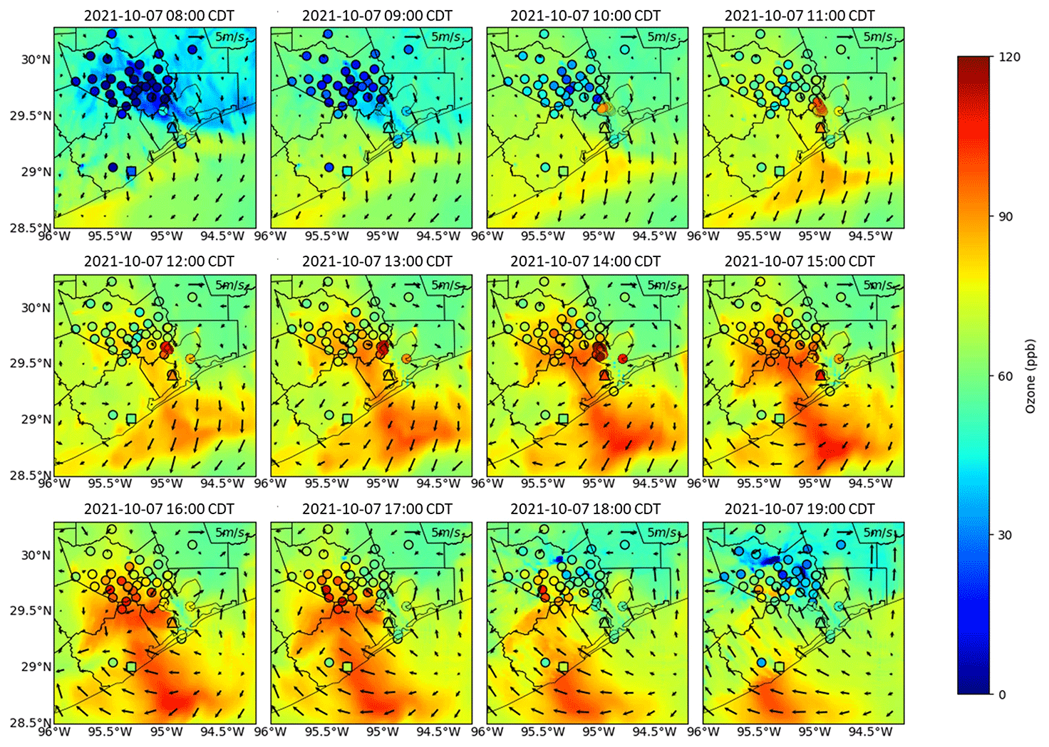
Figure 11Same as Fig. 8 but on 7 October, with the squares and triangles representing the Oyster Creek and Texas city CAMS sites, respectively.
3.3.2 Case study of 7 October 2021
On 7 October, the pontoon boat observed the highest 1 min O3 concentration (135 ppb) throughout the entire campaign period. This day started with weak northwesterly winds in the morning under post-frontal conditions, leading to high-O3 concentrations along the Gulf Coast (Fig. 11). The winds transitioned to northeasterly near 11:00 CDT (Fig. 12b), marking the onset of the Galveston Bay breeze at the pontoon and shrimp boat and the Texas city site (triangle label in Fig. 11) and the Gulf breeze at the Oyster Creek site (square label in Fig. 11), both accompanied by an increase in the O3 (Fig. 12a) and wind speed (Fig. 12c). By contrast, the model predicted a late onset of the Galveston Bay/Gulf breezes by 2–3 h, with a generally higher wind speed than was observed. Afterward, the wind directions further shifted from the east to southeast between 14:00 to 18:00 CDT, as the Gulf breezes propagated to all four locations in Fig. 12b, causing the highest-O3 mixing ratios therein. Similarly, the model overestimated the Gulf breeze intensity, leading to the underestimation of O3 at the three locations along Galveston Bay. The model also continuously overestimated the moderate level of O3 (60–70 ppb) at the Oyster Creek site under the Gulf breeze from 11:00 to 20:00 CDT, implying that the lifetime of O3 or its precursors over water was likely overpredicted. Different from 9 September, the process analysis on this local-scale event indicates that CHEM is the major process that leads to high-O3 concentrations over the Gulf of Mexico (Fig. S10 in the Supplement). ADV only contributes to the increase in the O3 at 08:00–09:00 CDT, corresponding to the offshore transport of O3 in the morning under northwesterly winds.
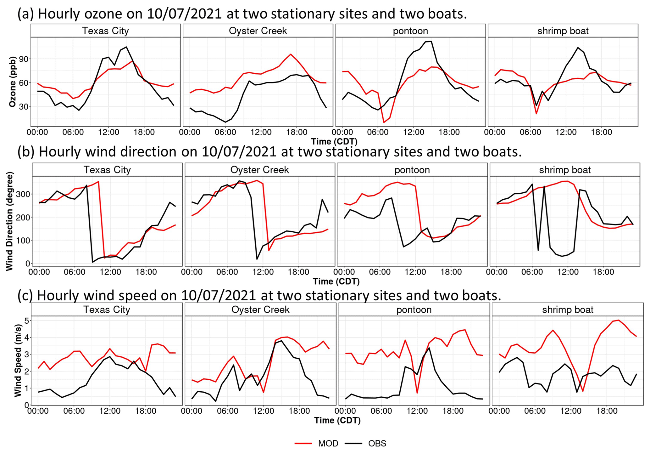
Figure 12Same as Fig. 10 but on 7 October, with the Texas city (triangles in Fig. 11) and Oyster Creek (squares in Fig. 11) CAMS sites and two boats.
To sum up, the high-O3 event on 7 October was related to the mesoscale Galveston Bay and Gulf breeze recirculation. Two boats and the Texas city site captured the start of the Bay breeze at ∼ 11:00 CDT and the development of the Gulf breeze at 14:00–18:00 CDT, the latter of which leads to peak hourly O3 by bringing the aged O3 and emissions back to land. Affected continuously by the Gulf breeze from 11:00 to 20:00 CDT, O3 at the Oyster Creek site stayed at 60–70 ppb. The model predicts the onset of the Bay and Gulf breezes 2–3 h late, with higher wind speed, causing the delayed and lower-O3 peaks along Galveston Bay.
As part of the TRACER-AQ 2021 field campaign in the Houston area, three boats, a UH pontoon boat, and two commercial vessels equipped with an automatic sampling system and ozonesonde launches were deployed in Galveston Bay and the Gulf of Mexico from July to October. The resulting datasets, including the surface and vertical O3 concentrations and various meteorological parameters, provide a unique opportunity to evaluate the performance of TCEQ's regulatory WRF–CAMx modeling system, regarding its ability to capture the high offshore O3 events. Driven by the optimized WRF meteorological outputs, the CAMx model can satisfactorily capture the spatiotemporal variability in the daytime O3 for the three boats (R > 0.70), with an overall 4–8 ppb (9 %–22 %) overestimation mainly caused by the high positive biases on clean days. During high-O3 events, the model tends to underestimate O3 by 5 ppb near the surface and by 10 ppb up to 4 km aloft.
The reasonable model performance provides credibility for relying on the model's process analysis tool to investigate the factors responsible for the high-O3 episodes over the Gulf of Mexico. The results show that O3 chemistry is the major process leading to high-O3 concentrations relative to clean conditions. A region-wide increase in the long-lived VOC species through advection, such as paraffin, formaldehyde, and acetaldehyde, accelerated O3 production rates under a NOx-limited regime. In the meantime, the enhanced VOCs can produce more O3 near western Galveston Bay and off the Gulf Coast under high-NOx concentrations brought by the northeasterly winds from the Houston Ship Channel. Thus, the higher-O3 chemical production over water can be from both NOx- and VOC-limited regimes.
Two cases, 9 September and 7 October, were then selected to illustrate the development of high-O3 events further. Both cases involved north–northeast morning winds transporting the inland emissions toward the sea, shifting to the east–southeast in the afternoon, and transporting the offshore O3 and its precursors to the land. Therefore, well-represented wind conditions are of great importance for air quality models to accurately capture the timing and magnitude of elevated O3 levels in these cases. However, the two cases differ in terms of atmospheric scale. The event on 9 September was influenced by a large-scale circulation with regionally homogeneous wind conditions. The easterly winds in the afternoon brought a second air plume from the eastern boundary of the domain, following the first locally produced plume, illustrating the contributions of regional advection, in addition to chemistry, to the high-O3 mixing ratios in this case. Conversely, the 7 October case was dominated by the mesoscale development of Galveston Bay and Gulf breezes, characterized by a generally lower wind speed and higher-O3 level. Double O3 peaks can also be observed near Galveston Bay, such as the Texas city site in this case, corresponding to the arrival of the Galveston Bay and Gulf breezes, respectively. The model wrongly predicted the timing of the wind direction shift and overestimated the wind speed in both cases, leading to the temporally mismatched and numerically buffered O3 peaks.
This study reveals the important role of chemical O3 production over Galveston Bay and the Gulf of Mexico from precursors emitted from the adjacent land and the Houston Ship Channel or transported regionally from the northeastern states. The high O3 produced offshore can then be transported back to land and cause O3 exceedances at the air quality monitors. Therefore, local and regional emissions need to be stringently regulated to reduce the frequency of such events. Additionally, wind conditions are critical meteorological factors leading to these high-O3 episodes and thus need to be well represented in photochemical models to have an accurate air quality forecast in urban coastal regions.
CAMx and WRF models are publicly available at https://camx-wp.azurewebsites.net/getmedia/CAMx_v7.10.src.210105.tgz (RAMBOLL, 2021) and https://doi.org/10.5065/D68S4MVH (Skamarock et al., 2008), respectively. CAMS data can be downloaded from the TAMIS web interface (https://www17.tceq.texas.gov/tamis/index.cfm?fuseaction=home.welcome, TCEQ, 2002), and other campaign data are archived on the TRACER-AQ website (https://www-air.larc.nasa.gov/cgi-bin/ArcView/traceraq.2021, NASA, 2021).
The supplement related to this article is available online at: https://doi.org/10.5194/acp-23-13685-2023-supplement.
YW conceived the research idea. WL, XL, and ES conducted the model simulation. TG, JF, and PW provided the field observations. WL performed the data analysis and drafted the initial paper. All authors contributed to the interpretation of the results and the preparation of the paper.
The contact author has declared that none of the authors has any competing interests.
The findings, opinions, and conclusions are the work of the author(s) and do not necessarily represent the findings, opinions, or conclusions of the TCEQ or AQRP.
Publisher's note: Copernicus Publications remains neutral with regard to jurisdictional claims made in the text, published maps, institutional affiliations, or any other geographical representation in this paper. While Copernicus Publications makes every effort to include appropriate place names, the final responsibility lies with the authors.
We acknowledge the individuals and groups who collected and shared the TRACER-AQ 2021 filed campaign datasets.
This research has been supported by the Texas Commission on Environmental Quality (grant no. 582-22-31544-019) and the Texas Air Quality Research Program (AQRP; grant no. 22-008).
This paper was edited by Suvarna Fadnavis and reviewed by two anonymous referees.
Abdi-Oskouei, M., Carmichael, G., Christiansen, M., Ferrada, G., Roozitalab, B., Sobhani, N., Wade, K., Czarnetzki, A., Pierce, R. B., Wagner, T., and Stanier, C.: Sensitivity of Meteorological Skill to Selection of WRF-Chem Physical Parameterizations and Impact on Ozone Prediction During the Lake Michigan Ozone Study (LMOS), J. Geophys. Res.-Atmos., 125, e2019JD031971, https://doi.org/10.1029/2019JD031971, 2020.
Abdi-Oskouei, M., Roozitalab, B., Stanier, C. O., Christiansen, M., Pfister, G., Pierce, R. B., McDonald, B. C., Adelman, Z., Janseen, M., Dickens, A. F., and Carmichael, G. R.: The Impact of Volatile Chemical Products, Other VOCs, and NOx on Peak Ozone in the Lake Michigan Region, J. Geophys. Res.-Atmos., 127, e2022JD037042, https://doi.org/10.1029/2022JD037042, 2022.
Baker, K. R., Liljegren, J., Valin, L., Judd, L., Szykman, J., Millet, D. B., Czarnetzki, A., Whitehill, A., Murphy, B., and Stanier, C.: Photochemical model representation of ozone and precursors during the 2017 Lake Michigan ozone study (LMOS), Atmos. Environ., 293, 119465, https://doi.org/10.1016/j.atmosenv.2022.119465, 2023.
Banta, R. M., Senff, C. J., Nielsen-Gammon, J., Darby, L. S., Ryerson, T. B., Alvarez, R. J., Sandberg, S. P., Williams, E. J., and Trainer, M.: A Bad Air Day in Houston, B. Am. Meteorol. Soc., 86, 657–670, https://doi.org/10.1175/BAMS-86-5-657, 2005.
Bernier, C., Wang, Y., Gronoff, G., Berkoff, T., Knowland, K. E., Sullivan, J. T., Delgado, R., Caicedo, V., and Carroll, B.: Cluster-based characterization of multi-dimensional tropospheric ozone variability in coastal regions: an analysis of lidar measurements and model results, Atmos. Chem. Phys., 22, 15313–15331, https://doi.org/10.5194/acp-22-15313-2022, 2022.
Burkholder, J. B., Sander, S. P., Abbatt, J. P. D. A. D., Barker, J. R., Huie, R. E., Kolb, C. E., Iii, M. J. K., Orkin, V. L., Wilmouth, D. M., and Wine, P. H.: Chemical Kinetics and Photochemical Data for Use in Atmospheric Studies: Evaluation number 18, JPL Publ. 15-10, Jet Propulsion Laboratory, Pasadena, CA, 2019.
Caicedo, V., Rappenglueck, B., Cuchiara, G., Flynn, J., Ferrare, R., Scarino, A. J., Berkoff, T., Senff, C., Langford, A., and Lefer, B.: Bay Breeze and Sea Breeze Circulation Impacts on the Planetary Boundary Layer and Air Quality From an Observed and Modeled DISCOVER-AQ Texas Case Study, J. Geophys. Res.-Atmos., 124, 7359–7378, https://doi.org/10.1029/2019JD030523, 2019.
Chen, F. and Dudhia, J.: Coupling an Advanced Land Surface–Hydrology Model with the Penn State–NCAR MM5 Modeling System. Part I: Model Implementation and Sensitivity, Mon. Weather Rev., 129, 569–585, https://doi.org/10.1175/1520-0493(2001)129<0569:CAALSH>2.0.CO;2, 2001.
Dacic, N., Sullivan, J. T., Knowland, K. E., Wolfe, G. M., Oman, L. D., Berkoff, T. A., and Gronoff, G. P.: Evaluation of NASA's high-resolution global composition simulations: Understanding a pollution event in the Chesapeake Bay during the summer 2017 OWLETS campaign, Atmos. Environ., 222, 117133, https://doi.org/10.1016/j.atmosenv.2019.117133, 2020.
Darby, L. S.: Cluster Analysis of Surface Winds in Houston, Texas, and the Impact of Wind Patterns on Ozone, J. Appl. Meteorol. Clim., 44, 1788–1806, https://doi.org/10.1175/JAM2320.1, 2005.
Dreessen, J., Orozco, D., Boyle, J., Szymborski, J., Lee, P., Flores, A., and Sakai, R. K.: Observed ozone over the Chesapeake Bay land-water interface: The Hart-Miller Island Pilot Project, J. Air Waste Manage., 69, 1312–1330, https://doi.org/10.1080/10962247.2019.1668497, 2019.
Dreessen, J., Ren, X., Gardner, D., Green, K., Stratton, P., Sullivan, J. T., Delgado, R., Dickerson, R. R., Woodman, M., Berkoff, T., Gronoff, G., and Ring, A.: VOC and trace gas measurements and ozone chemistry over the Chesapeake Bay during OWLETS-2, 2018, J. Air Waste Manage., 73, 178–199, https://doi.org/10.1080/10962247.2022.2136782, 2023.
Dye, T. S., Roberts, P. T., and Korc, M. E.: Observations of Transport Processes for Ozone and Ozone Precursors during the 1991 Lake Michigan Ozone Study, J. Appl. Meteorol. Clim., 34, 1877–1889, https://doi.org/10.1175/1520-0450(1995)034<1877:OOTPFO>2.0.CO;2, 1995.
Foken, T.: 50 Years of the Monin–Obukhov Similarity Theory, Bound.-Lay. Meteorol., 119, 431–447, https://doi.org/10.1007/s10546-006-9048-6, 2006.
Goldberg, D. L., Loughner, C. P., Tzortziou, M., Stehr, J. W., Pickering, K. E., Marufu, L. T., and Dickerson, R. R.: Higher surface ozone concentrations over the Chesapeake Bay than over the adjacent land: Observations and models from the DISCOVER-AQ and CBODAQ campaigns, Atmos. Environ., 84, 9–19, https://doi.org/10.1016/j.atmosenv.2013.11.008, 2014.
Griggs, T., Flynn, J., Wang, Y., Alvarez, S., Comas, M., and Walter, P.: Characterizing Over-Water High Ozone Events in the Houston–Galveston–Brazoria Region During July–October 2021, B. Am. Meteorol. Soc., submitted, 2023.
Iacono, M. J., Delamere, J. S., Mlawer, E. J., Shephard, M. W., Clough, S. A., and Collins, W. D.: Radiative forcing by long-lived greenhouse gases: Calculations with the AER radiative transfer models, J. Geophys. Res.-Atmos., 113, D13103, https://doi.org/10.1029/2008JD009944, 2008.
Kommalapati, R. R., Liang, Z., and Huque, Z.: Photochemical model simulations of air quality for Houston–Galveston–Brazoria area and analysis of ozone–NOx–hydrocarbon sensitivity, Int. J. Environ. Sci. Te., 13, 209–220, https://doi.org/10.1007/s13762-015-0862-6, 2016.
Leuchner, M. and Rappenglück, B.: VOC source–receptor relationships in Houston during TexAQS-II, Atmos. Environ., 44, 4056–4067, https://doi.org/10.1016/j.atmosenv.2009.02.029, 2010.
Li, W., Wang, Y., Bernier, C., and Estes, M.: Identification of Sea Breeze Recirculation and Its Effects on Ozone in Houston, TX, During DISCOVER-AQ 2013, J. Geophys. Res.-Atmos., 125, e2020JD033165, https://doi.org/10.1029/2020JD033165, 2020.
Li, X. and Rappenglück, B.: A WRF–CMAQ study on spring time vertical ozone structure in Southeast Texas, Atmos. Environ., 97, 363–385, https://doi.org/10.1016/j.atmosenv.2014.08.036, 2014.
Liu, X., Wang, Y., Wasti, S., Li, W., Soleimanian, E., Flynn, J., Griggs, T., Alvarez, S., Sullivan, J. T., Roots, M., Twigg, L., Gronoff, G., Berkoff, T., Walter, P., Estes, M., Hair, J. W., Shingler, T., Scarino, A. J., Fenn, M., and Judd, L.: Evaluating WRF-GC v2.0 predictions of boundary layer and vertical ozone profiles during the 2021 TRACER-AQ campaign in Houston, Texas, EGUsphere [preprint], https://doi.org/10.5194/egusphere-2023-892, 2023.
Mazzuca, G. M., Ren, X., Loughner, C. P., Estes, M., Crawford, J. H., Pickering, K. E., Weinheimer, A. J., and Dickerson, R. R.: Ozone production and its sensitivity to NOx and VOCs: results from the DISCOVER-AQ field experiment, Houston 2013, Atmos. Chem. Phys., 16, 14463–14474, https://doi.org/10.5194/acp-16-14463-2016, 2016.
Misenis, C. and Zhang, Y.: An examination of sensitivity of WRF/Chem predictions to physical parameterizations, horizontal grid spacing, and nesting options, Atmos. Res., 97, 315–334, https://doi.org/10.1016/j.atmosres.2010.04.005, 2010.
Morrison, H., Thompson, G., and Tatarskii, V.: Impact of Cloud Microphysics on the Development of Trailing Stratiform Precipitation in a Simulated Squall Line: Comparison of One- and Two-Moment Schemes, Mon. Weather Rev., 137, 991–1007, https://doi.org/10.1175/2008MWR2556.1, 2009.
Nakanishi, M. and Niino, H.: Development of an Improved Turbulence Closure Model for the Atmospheric Boundary Layer, J. Meteorol. Soc. Jpn. Ser. II, 87, 895–912, https://doi.org/10.2151/jmsj.87.895, 2009.
NASA: Data archive for the TRACER-AQ 2021 field campaign, Langely Recerch Center [data set], https://www-air.larc.nasa.gov/cgi-bin/ArcView/traceraq.2021 (last access: 27 October 2023), 2021.
Ngan, F. and Byun, D.: Classification of Weather Patterns and Associated Trajectories of High-Ozone Episodes in the Houston–Galveston–Brazoria Area during the 2005/06 TexAQS-II, J. Appl. Meteorol. Clim., 50, 485–499, https://doi.org/10.1175/2010JAMC2483.1, 2011.
Nonattainment Areas for Criteria Pollutants (Green Book): https://www.epa.gov/green-book (last access: 6 January 2023), 2023.
Pan, S., Choi, Y., Roy, A., Li, X., Jeon, W., and Souri, A. H.: Modeling the uncertainty of several VOC and its impact on simulated VOC and ozone in Houston, Texas, Atmos. Environ., 120, 404–416, https://doi.org/10.1016/j.atmosenv.2015.09.029, 2015.
Pan, S., Choi, Y., Roy, A., and Jeon, W.: Allocating emissions to 4 km and 1 km horizontal spatial resolutions and its impact on simulated NOx and O3 in Houston, TX, Atmos. Environ., 164, 398–415, https://doi.org/10.1016/j.atmosenv.2017.06.026, 2017.
RAMBOLL: CMAx version 7.10, RAMBOLL [code], https://camx-wp.azurewebsites.net/getmedia/CAMx_v7.10.src.210105.tgz (last access: 27 October 2023), 2021.
Rappenglück, B., Perna, R., Zhong, S., and Morris, G. A.: An analysis of the vertical structure of the atmosphere and the upper-level meteorology and their impact on surface ozone levels in Houston, Texas, J. Geophys. Res.-Atmos., 113, D17315, https://doi.org/10.1029/2007JD009745, 2008.
Sillman, S.: The use of NOy, H2O2, and HNO3 as indicators for ozone-NOmathitx -hydrocarbon sensitivity in urban locations, J. Geophys. Res.-Atmos., 100, 14175–14188, https://doi.org/10.1029/94JD02953, 1995.
Skamarock, W. C., Klemp, J. B., Dudhia, J., Gill, D. O., Barker, D. M., Duda, M. G., Huang, X. Y., Wang, W., and Powers, J. G.: A description of the advanced research WRF version 3 (No. NCAR/TN-475+STR), University Corporation for Atmospheric Research, technical note, 475, p. 113, https://doi.org/10.5065/D68S4MVH, 2008.
Soleimanian, E., Wang, Y., and Estes, M.: Long-term trend in surface ozone in Houston-Galveston-Brazoria: Sectoral contributions based on changes in volatile organic compounds, Environ. Pollut., 308, 119647, https://doi.org/10.1016/j.envpol.2022.119647, 2022.
Soleimanian, E., Wang, Y., Li, W., Liu, X., Griggs, T., Flynn, J., Walter, P. J., and Estes, M. J.: Understanding ozone episodes during the TRACER-AQ campaign in Houston, Texas: The role of transport and ozone production sensitivity to precursors, Sci. Total Environ., 900, 165881, https://doi.org/10.1016/j.scitotenv.2023.165881, 2023.
Sullivan, J. T., Berkoff, T., Gronoff, G., Knepp, T., Pippin, M., Allen, D., Twigg, L., Swap, R., Tzortziou, M., Thompson, A. M., Stauffer, R. M., Wolfe, G. M., Flynn, J., Pusede, S. E., Judd, L. M., Moore, W., Baker, B. D., Al-Saadi, J., and McGee, T. J.: The Ozone Water–Land Environmental Transition Study: An Innovative Strategy for Understanding Chesapeake Bay Pollution Events, B. Am. Meteorol. Soc., 100, 291–306, https://doi.org/10.1175/BAMS-D-18-0025.1, 2019.
TCEQ: The Texas Air Monitoring Information 81 System (TAMIS) website, TCEQ, https://www17.tceq.texas.gov/tamis/index.cfm?fuseaction=home.welcome (last access: 27 October 2023), 2002.
Wesely, M. L.: Parameterization of surface resistances to gaseous dry deposition in regional-scale numerical models, Atmos. Environ., 41, 52–63, https://doi.org/10.1016/j.atmosenv.2007.10.058, 1989.
Xiao, X., Cohan, D. S., Byun, D. W., and Ngan, F.: Highly nonlinear ozone formation in the Houston region and implications for emission controls, J. Geophys. Res.-Atmos., 115, D23309, https://doi.org/10.1029/2010JD014435, 2010.
Yu, S., Mathur, R., Pleim, J., Pouliot, G., Wong, D., Eder, B., Schere, K., Gilliam, R., and Trivikrama Rao, S.: Comparative evaluation of the impact of WRF–NMM and WRF–ARW meteorology on CMAQ simulations for O3 and related species during the 2006 TexAQS/GoMACCS campaign, Atmos. Pollut. Res., 3, 149–162, https://doi.org/10.5094/APR.2012.015, 2012.
Zhang, C., Wang, Y., and Hamilton, K.: Improved Representation of Boundary Layer Clouds over the Southeast Pacific in ARW-WRF Using a Modified Tiedtke Cumulus Parameterization Scheme, Mon. Weather Rev., 139, 3489–3513, https://doi.org/10.1175/MWR-D-10-05091.1, 2011.