Signatures of the Madden–Julian oscillation in middle-atmosphere zonal mean temperature: triggering the interhemispheric coupling pattern

The influence of the Madden–Julian oscillation (MJO) on the middle atmosphere (MA) and particularly on MA temperature is of interest for both the understanding of MJO-induced teleconnections and research on the variability of the MA. We analyze statistically the connection of the MJO and the MA zonal mean temperature based on observations by the Microwave Limb Sounder (MLS) satellite instrument. We consider all eight MJO phases, different seasons and the state of the quasi-biennial oscillation (QBO). We show that MA temperature anomalies are significantly related to the MJO and its temporal development. The MJO signal in the zonal mean MA temperature is characterized by a particular spatial pattern in the MA, which we link to the interhemispheric coupling (IHC) mechanism, as a major outcome of this study. The signal with the largest magnitude is found in the polar MA during boreal winter with temperature deviations on the order of ±10 K when the QBO at 50 hPa is in its easterly phase. Other atmospheric conditions and locations also exhibit temperature signals, which are, however, weaker or noisier. We also analyze the change in the temperature signal while the MJO progresses from one phase to the next. We find a gradual altitude shift in parts of the IHC pattern, which can be seen more or less clearly depending on the atmospheric conditions.

The statistical link between the MJO and the MA temperature highlights illustratively the far-reaching connections across different atmospheric layers and geographical regions in the atmosphere. Additionally, it highlights close linkages of known dynamical features of the atmosphere, particularly the MJO, the IHC, the QBO and sudden stratospheric warmings (SSWs). Because of the wide coverage of atmospheric regions and included dynamical features, the results might help to further constrain the underlying dynamical mechanisms and could be used as a benchmark for the representation of atmospheric couplings on the intraseasonal timescale in atmospheric models.

1 Introduction

The Madden–Julian oscillation (MJO), first documented by Madden and Julian (1972), is known as the dominant mode of intraseasonal variability in the tropical troposphere (Zhang, 2005). It is a highly variable feature of the atmosphere, so that, e.g., its period varies strongly between about 30 and 90 d (Zhang, 2005). Its appearance influences weather patterns in many equatorial regions, e.g., the monsoons in Asia and Australia (Zhang, 2005).

Dynamical anomalies connected to the MJO are measured around the whole Equator (e.g., Cassou, 2008). Moreover, the MJO also has influences around the whole globe and is itself influenced by extratropical regions, making the MJO a component of global teleconnection patterns (Lau and Waliser, 2012, Chap. 14). For a review of the observed teleconnections between the tropics and the polar regions on different timescales, see, e.g., Yuan et al. (2018).

Due to the intraseasonal timescale on which the MJO acts, deeper knowledge on the processes that control it is expected to improve the forecast skills of longer-term weather forecasts (e.g., Zhang, 2013). The understanding of the mechanisms of the teleconnections is important for improving the representation of the MJO in models but might in turn also help to improve the forecast skills in the extratropics, e.g., in terms of the prediction of extreme weather events (Lau and Waliser, 2012, Chap. 14).

Garfinkel et al. (2012) proposed a special mechanism for MJO-related teleconnections that considers the propagation of Rossby waves into the stratosphere. These waves could influence the polar vortex and modulate the appearance of midwinter major sudden stratospheric warmings (SSWs), so that SSWs follow certain MJO phases. It was already known that the occurrence of SSWs during Arctic winter can then influence the tropospheric state below (e.g., Baldwin and Dunkerton, 2001).

There is also increasing evidence that the variability of the MJO itself is partly controlled by the stratosphere. A prominent example of this is the influence of the quasi-biennial oscillation (QBO) during boreal winter: Yoo and Son (2016) found that the MJO amplitude tends to be larger during the QBO easterly phase and smaller during the QBO westerly phase, and several studies followed up on this (e.g., Son et al., 2017; Marshall et al., 2017; Zhang and Zhang, 2018; Densmore et al., 2019; Wang and Wang, 2021). The influence on the MJO from above is also covered by a more general recent review by Haynes et al. (2021).

Consequently, there is increasing awareness of the potential of considering troposphere–stratosphere couplings in both directions in weather prediction systems, as shown by, e.g., Domeisen et al. (2020). In addition, at least from these examples, it becomes clear that it is of importance to consider at least the stratosphere to completely understand the functioning of the MJO in the climate system.

In addition to this troposphere-related motivation, there is a second major motivation to study the connection of the MJO and the middle atmosphere (MA), which arises from the interest in the variability of the MA itself. A major aim is the disentanglement of all the sources of temperature variability, e.g., solar variability (e.g., Gray et al., 2010), volcanic eruptions (e.g., Timmreck, 2012), anthropogenic climate change (e.g., Randel et al., 2009; Santer et al., 2013; Maycock et al., 2018; Beig et al., 2003; Beig, 2011) and the change in stratospheric ozone. In order to increase the robustness of those analyses, the smaller sources of temperature variability should also be known and quantified.

The MJO has, to our knowledge, gotten only little attention as one possible independent source of temperature variability in the MA. In addition to the already mentioned analysis by Garfinkel et al. (2012), the studies by Yang et al. (2017, 2019) are in this context of relevance for our analysis. They are mostly based on modeled and reanalyzed data, whereas it is our aim to provide a purely observational perspective. Sun et al. (2021) analyze the effect of the MJO on the northern mesosphere during boreal winter. They also mostly rely on modeled data but use satellite observations as support, in particular, the same observational dataset as we use in the following (Sect. 2.1). There are more studies relevant in the broader context, but either they do not treat the influence on temperature as the main point (e.g., Moss et al., 2016; Tsuchiya et al., 2016; Wang et al., 2018a) or they are limited to different atmospheric regions (e.g., Yang et al., 2018; Kumari et al., 2020, 2021).

We note as an additional aspect for the motivation that the occurrence rates of individual MJO phases appear to be subject to climate change (Yoo et al., 2011). Therefore, a linkage of the MJO and the MA could represent an additional pathway of anthropogenic climate change into the MA. Conversely, the characterization of the MJO–MA relationship might also be helpful for understanding climate-change-related changes in the teleconnection patterns mentioned above.

Most related studies first determine the MJO phase with the strongest response and mostly concentrate in the following analysis on this phase (e.g., Garfinkel et al., 2012; Yang et al., 2017). The temporal evolution of the atmosphere is then considered in time lags around the appearance of this phase. We instead consider all eight MJO phases, so that the transition of the MA temperature response from one MJO phase to the next becomes visible. Furthermore, we concentrate in this paper on the analysis of zonal mean temperatures.

The paper contains a description of the datasets and methodology in Sect. 2. The results, i.e., the zonal mean MA temperature responses to the individual MJO phases for different atmospheric conditions, are shown in Sect. 3. Section 4 contains an extensive discussion, in which the results are related to known dynamical features of the MA, before we conclude the paper in Sect. 5

2 Datasets and analysis approach

2.1 Datasets

We analyze the temperature data product measured by NASA's Microwave Limb Sounder (MLS) on the Aura satellite (Schwartz et al., 2020), version 5. A previous version of the dataset was validated by Schwartz et al. (2008). Differences to the new version are mentioned in Livesey et al. (2020). Data screening and exclusion have been performed according to all suggestions in the MLS quality document (Livesey et al., 2020), including the screening for cloud effects based on the MLS ice water content (IWC) product. We analyze the complete reasonable vertical range from 261 to 0.00046 hPa and also use the complete temporal coverage of the ongoing measurements of about 17 years at the time of the analysis (approximately August 2004 to September 2021). The data have a spatial resolution that roughly decreases with height in a range from about 4 km vertical and 170 km horizontal resolution at 261 hPa to 13 km vertical and 316 km horizontal resolution at 0.00046 hPa (Livesey et al., 2020). The data have been analyzed on the original pressure grid. One has to keep in mind that the analysis grid is finer than the varying vertical resolution and that adjacent altitudes are not completely independent of each other. The original data follow the satellite track and have been averaged to fit onto temporally and horizontally regular grids. In particular, for this paper we apply a zonal averaging with 10^∘ resolution in the latitudinal direction.

For the characterization of the MJO, we use the OLR-based MJO Index (OMI; OLR stands for outgoing longwave radiation) introduced by Kiladis et al. (2014). We calculate the OMI values from OLR using the open-source OMI calculation package (Hoffmann et al., 2021; Hoffmann, 2021), version 1.2.2. According to Hoffmann et al. (2021), a high agreement with the original calculation routine, which is close to being identical, is expected. For the calculation, interpolated OLR data according to Liebmann and Smith (1996) have been used. From the two OMI values per time step, the phase and the strength of the MJO for each day can easily be calculated following the phase diagrams in Kiladis et al. (2014) and Wheeler and Hendon (2004).

We note that the MJO is subject to seasonal variability (e.g., Zhang, 2005). The common MJO concept with the characteristic eastward propagation applies best for boreal winter. During boreal summer, the propagation direction includes a northward component (e.g., Wang et al., 2018b), and the feature is often given a distinct name, the boreal summer intraseasonal oscillation (BSISO). This also has implications for the definition of appropriate MJO indices, and partly, particular BSISO indices are used for analyses with a special focus on boreal summer (e.g., Kikuchi et al., 2012). However, since our analysis is not restricted to boreal summer and Wang et al. (2018b) state that the MJO index OMI is also capable of reasonably tracking the BSISO, we apply OMI consistently for all seasons. This has the advantage of comparability of the results for different seasons.

For the characterization of the QBO, we use monthly mean zonal wind data above Singapore at 50 hPa (Naujokat, 1986). We apply the simplest discrimination approach: positive zonal wind values indicate a QBO westerly phase and negative values a QBO easterly phase.

2.2 Approach

Our analysis approach is a superposed epoch analysis (SEA), also known as a composite analysis. The complete analysis chain consists, however, of several steps, which are computed for each geolocation of the previously mentioned regular spatial grid separately.

First, a temperature anomaly is computed by applying a centered boxcar running average with a window length of 90 d as a low-pass filter and calculating the difference between the original and low-pass-filtered time series. Afterwards the anomaly is smoothed with a 10 d running average. The latter is mainly done for reasons of comparability with other analyses and is strictly speaking disadvantageous since it introduces a statistical dependence of the previously independent individual days. Therefore, we have checked that, in practice, the results do not change significantly when the 10 d filter is not applied. The resulting anomaly time series contains, due to the filtering, only strongly damped variations on much longer (e.g., the seasonal cycle) and much shorter (e.g., weather fluctuations) timescales than the MJO but still captures a broad range of frequencies on the intraseasonal timescale relevant to the MJO.

Second, the data are selected according to the environmental conditions. We only consider those days when the strength of the MJO is greater than 1. Values between 1 and 1.5 are common choices in many MJO-related studies to make sure that there is actually an MJO signature (e.g., Hood, 2017; Garfinkel et al., 2012, 2014; Yang et al., 2017, 2019), whereas our choice of 1 includes as many days as possible. Depending on the particular experimental setups described below, the data are also selected with respect to particular seasons and with respect to the state of the QBO. Specifically, all days that do not match the wanted setup criteria are removed from the dataset prior to the SEA. We consider the seasons boreal winter and austral summer (December, January and February) and boreal summer and austral winter (June, July and August). The complete set of selection criteria for a particular experiment is sometimes called “atmospheric conditions” or similar in the remainder of the paper.

Third, the actual SEA is carried out: the selected temperature observations are grouped by the related MJO phases of each day and then averaged, so that one temperature mean value per MJO phase is calculated, complemented by the corresponding standard errors of the mean. The basic idea is that temperature fluctuations that are not correlated with the MJO phase propagation will average out, while fluctuations correlated with the MJO phases will add up, so that remaining epoch-averaged anomalies indicate a statistical connection between the MJO phase propagation and the MA temperature. Note that we apply a small correction after this basic step: a mean over the complete data subset at the respective geolocation (i.e., independent of the MJO phase) is subtracted from all eight average values. This overall mean value is usually close to 0 K, because the whole calculation is carried out on temperature anomalies, which are scattered around zero. However, the average of the selected subset of the data may slightly deviate from zero, which would complicate the comparison of the results for different geolocations if not corrected for. Figure 1 shows two examples of the SEA results, which represent a strong response and a weak response. The number of days that go into the individual averages depends of course strongly on the selection criteria but also somewhat on the geolocation and the MJO phase itself. Rough numbers are about 400 d per MJO phase if only the MJO strength filtering is applied, 100 d with additionally the seasonal selection and 50 d with a combined seasonal and QBO selection.

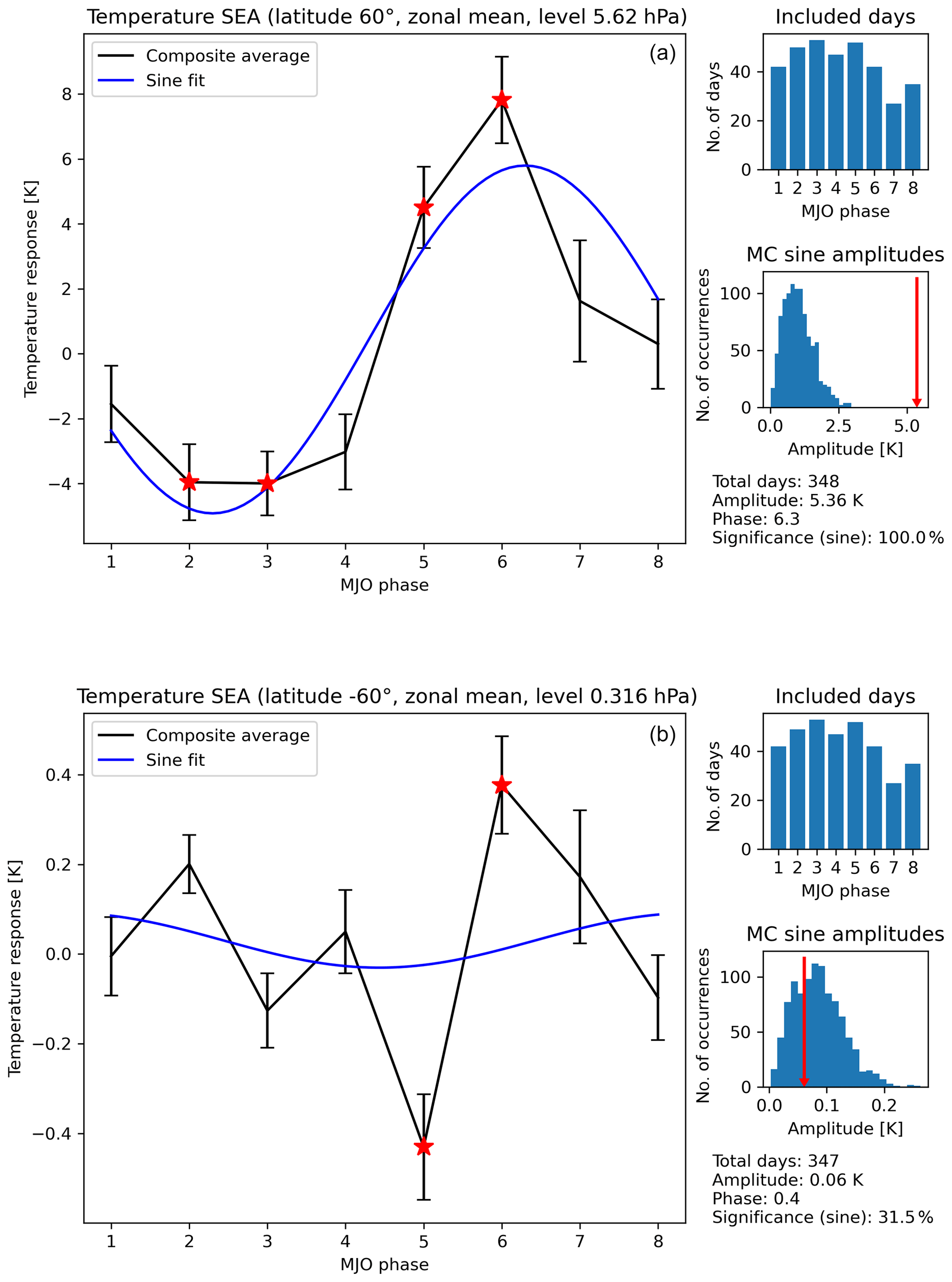
Figure 1 Examples of the temperature responses to the eight MJO phases at two geolocations for the boreal winter and QBO easterly situation. The examples have been selected for demonstration purposes to represent a particularly strong response (a) and a weak response (b). The following description applies to both cases. The main results, the average temperature anomalies for each MJO phase, are shown as the black lines in the larger panels together with the 8 standard errors of the mean shown as error bars. The blue line shows the fitted sine curve. Temperature responses, which are significant according to the MCIP method (see Sect. 2.2 for details on the MC quantification), are marked with red stars. Results according to the MCS significance estimation method, which estimates the significance of a systematic variation over all eight phases, are shown in the lower smaller panels on the right, respectively. The blue bars constitute a histogram of all sine amplitudes derived based on random data, whereas the sine amplitude of the real data is shown as a red arrow. The resulting percentage of random amplitudes lower than the real one is also given in the lower-right text field. The upper smaller panels on the right simply indicate how many days of the data went into each of the eight temperature anomaly average values.

As stated before (Sect. 1), we consider all eight phases of the MJO so that the transition of the MA temperature response from one phase to the other becomes visible. At least in an ideal case, the response could vary like a sine function over the course of the eight MJO phases. Following this notion, we fit a sine function to the eight mean values as the fourth analysis step to further characterize the behavior across the MJO phases. The parameters amplitude, phase and offset can freely be adjusted by the fit, whereas the period is fixed to eight MJO phases. The fit results can be analyzed with different foci. However, in this study, only the resulting amplitudes are used for a significance estimation in the next analysis step. The two examples in Fig. 1 also show the fitted sine curves. It is seen that the strong response indeed exhibits a sine-like behavior and the amplitude roughly represents the strength of the deviations, whereas the appearance of the weak response is noisier, which results in an even weaker sine amplitude.

The fifth and final step is a significance estimation using a Monte Carlo (MC) method. For this, the analysis is basically repeated multiple times, each time with randomly modified input data. The resulting distribution of artificial results can be used to estimate how likely a particular temperature response can be the result of random fluctuations instead of physical reasons. As we pointed out in Hoffmann and von Savigny (2019), there is a wide scope of individual decisions in the design of the MC calculations, which can influence the final significance estimation. In order to not distract the reader from the basic results, we concentrate here on only one version of the random data generation (as most other publications also do), which is very comparable to many previous publications. In particular, we randomly redistribute the MJO index time series 1000 times; i.e., the attribution of MJO phases and strengths to the individual days of the time series is changed. The temperature data thereby remain untouched. The SEA calculation is repeated for each random data realization, resulting in a distribution of possible temperature responses. While we only present one kind of random data generation, we still show two different kinds of the final quantification of the significance. The first one, abbreviated as MCIP for “Monte Carlo individual phases” in the following, is also best comparable to previous studies, particularly if they are focused on individual MJO phases. It is simply checked for each MJO phase separately if the absolute value of the real SEA anomaly result for a particular MJO phase is greater than 95 % of the absolute values of the responses based on random data. Hence, this significance estimation checks whether the derived SEA temperature anomaly is strong enough to be only very unlikely produced by random fluctuations for each MJO phase separately. Significant average values according to this method are marked with a red star in Fig. 1. An advantage is that this significance estimation exists separately for each MJO phase. However, this method has the disadvantage that it may underestimate significance. For example, if we consider the result for MJO phase 1 in Fig. 1a, the response is relatively close to 0 K, consequently also likely reproduced by random data and therefore not marked as significant. However, the development of the response over all eight MJO phases indicates that the response of phase 1 could be a part of an overall systematic variation, albeit approximately at the zero crossing of the variation. Therefore, we use a second quantification approach, abbreviated as MCS for “Monte Carlo sine” in the following, in which we check that the real amplitude of the fitted sine function is greater than 95 % of the fitted amplitudes based on the random data. Hence, this quantification approach evaluates the systematic behavior over all eight phases and is therefore also based on a larger number of samples (all days that go into the eight averages instead of only those that go into one specific average). Examples of the distributions of sine amplitudes are also given in the lower smaller plots in Fig. 1.

We would like to point out that the overall approach aims at establishing a statistical connection between the MJO phase evolution and the MA temperature without probing a causal or physical connection. Strictly speaking, the direction of an influence is also not checked. However, describing a statistical connection first helps to clearly define the observational aspects, which the ultimately sought physical mechanism has to cover. This is the basic aim of this study. The reader should keep this statistical nature of the analysis in mind for the whole paper independent of the particular wording. For example, if the verbs “influences” or “affects” are used together with the MJO effects on MA temperature, we always refer to our statistical approach.

3 Results: MJO signals in zonal mean MA temperature

3.1 Boreal winter and austral summer

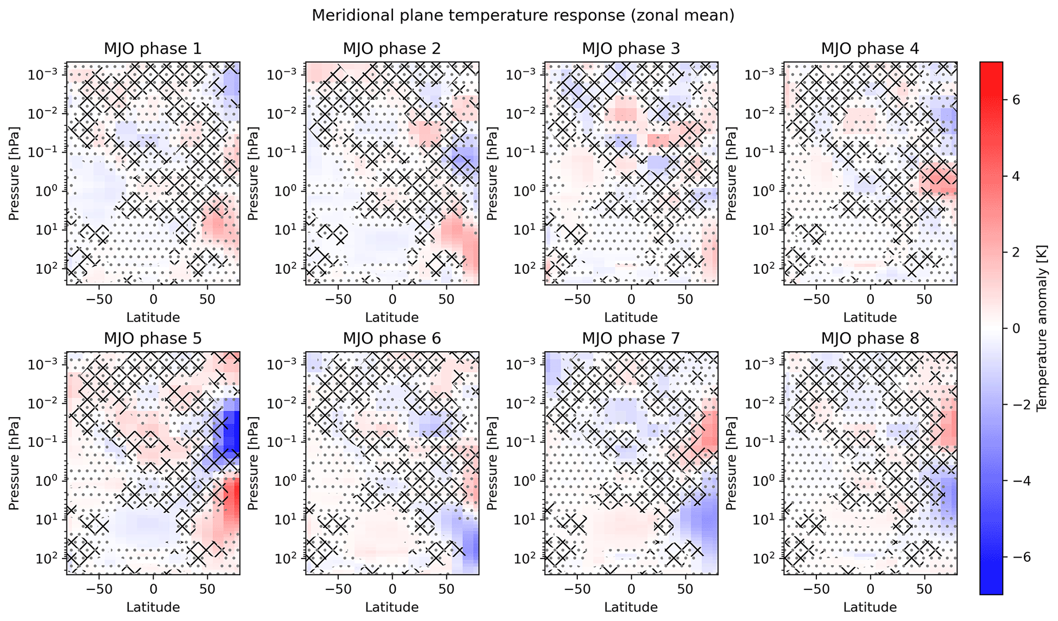
We start with the data restricted to boreal winter, since this season is the focus of many related studies (see Sect. 4). Figure 2 shows the meridional plane temperature responses for each of the eight MJO phases. The strongest response is seen for MJO phases 5 and 6 in the northern polar region, i.e., in the winter hemisphere. This response is spread vertically and divided into two zones with opposite signs visible as strong red and blue areas in the figure. The departures from the mean state are as high as ±6 K, even in this zonal mean picture.

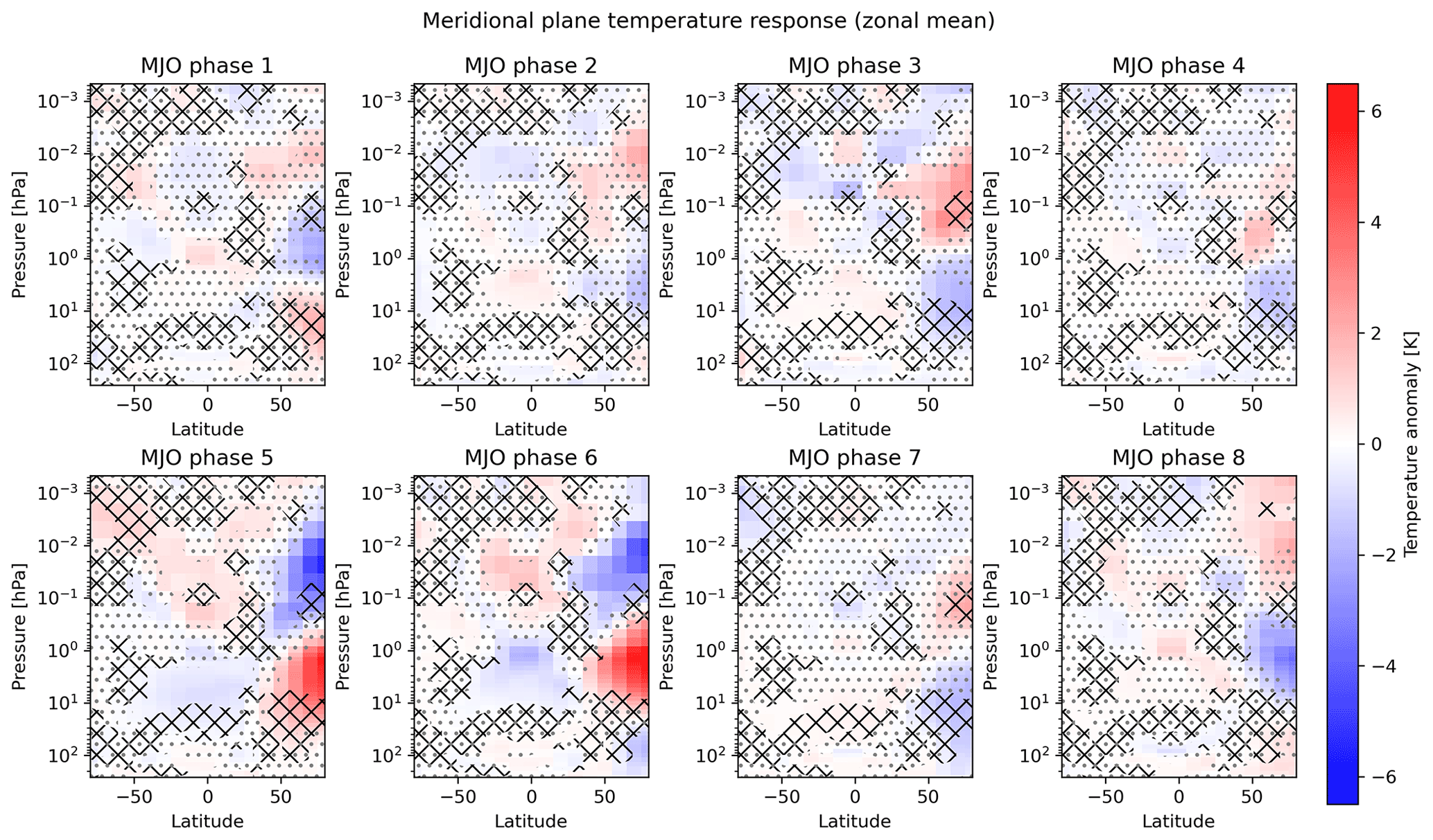
Figure 2 Meridional plane temperature responses for all eight MJO phases for the boreal winter or austral summer situation. Each panel contains the temperature anomaly response to a particular MJO phase for all geolocations in the zonal mean. All eight panels share the same color scale on the right. Insignificant values according to the MCIP method are marked with gray dots. Insignificant areas according to the MCS method are marked with black crossed lines. Note that the insignificance pattern according to the MCS method is identical for all eight MJO phases, since the overall systematic behavior is evaluated (slight differences in the hatches between the different panels are due to numerical inaccuracies in the rendering of the image and do not indicate differences in the significance estimation results).

A broader overall pattern in the meridional plane response can be recognized for most MJO phases. It is also clearest for MJO phase 5, so that these results are shown again with some visual guidance in Fig. 3 to support the following description. The two strong anomalies over the winter pole described before (indicated with dash-dotted circles in Fig. 3) constitute a vertical dipole with the positive anomaly around 3 hPa and the negative anomaly around about 0.03 hPa. This dipole is part of a remarkable global structure that comprises three more zones of spatially coherent anomalies. The departures from the mean state for these three zones are, at less than 1 K, much weaker than the polar ones but are still mostly significant, particularly when considering the MCS significance estimation. Two of these weaker anomalies constitute another vertical dipole at similar altitudes to the first one but are located around the Equator (indicated with dashed circles in Fig. 3). This equatorial dipole has an opposite sign compared to the polar dipole, so that all four zones together look like quadrupole spanning over the complete winter MA. In contrast, the fifth response zone is located at the summer polar latitudes (indicated with a solid circle in Fig. 3). It is even higher up between 0.01 and 0.001 hPa, and its extent is much smaller than the quadrupole pattern lower down. It shows a positive anomaly and looks like a polar summer mesosphere extension of the positive equatorial anomaly around 0.1 hPa. As we will come back to this pattern several times, we denote these MA anomalies temporarily as “five-zone signal” for a clearer identification in the following. However, we note that this pattern has already been described in the context of a dynamical feature in the MA, the interhemispheric coupling, as we will discuss in Sect. 4.1.

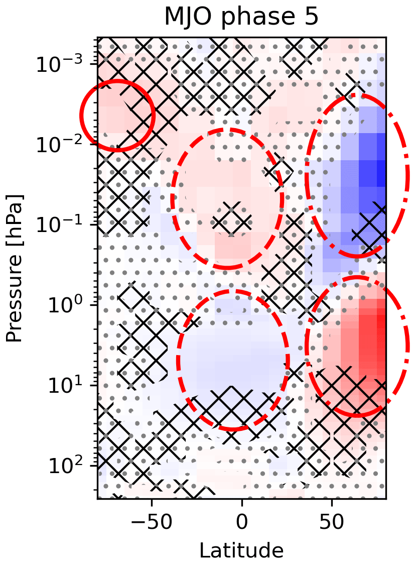
Figure 3 Repetition of the data shown for MJO phase 5 in Fig. 2 but with the five-zone signal highlighted to guide the reader better through the written description. The two dash–dotted circles indicate the two zones of the polar winter dipole in the temperature response. The two dashed circles mark the corresponding equatorial dipole, which has a reversed sign compared to the polar dipole. The solid circle marks the fifth anomaly zone located in the summer mesosphere, which has the same sign as the upper equatorial anomaly. See Sect. 3.1 for details.

The five-zone signal appears with varying clarity for each of the MJO phases but has an opposite sign for some phases (compare, e.g., the responses for phases 2 and 6 in Fig. 2). Of interest could therefore also be the transition of the response from one MJO phase to the next to get an idea of possible temporal systematics. For some of the phases, a gradual systematic change in the response is indeed recognizable, e.g., a downward shift of the polar winter dipole from MJO phase 2 to phase 4. Furthermore, some of the opposite MJO phases also show temperature responses with an opposing sign, as expected for an ideal temperature oscillation during the course of one MJO cycle (e.g., the previously mentioned phases 2 and 6). However, the mapping of the responses of opposite phases is not perfectly symmetric. We will elaborate on the aspect of the phase transition during the course of the following Sect. 3.2.

3.2 Boreal winter and austral summer and the state of the QBO

Figure 4 shows a similar analysis but with data selected for boreal winter and QBO easterly conditions. Overall, the responses look similar to those for boreal winter data (Fig. 2; note that the color scale has a different range). In particular, the five-zone signal is recognizable for each MJO phase, although the responses for MJO phases 1 and 8 look somewhat disturbed (which will become part of the interpretation below). The significant part of the summer mesosphere extension appears generally to be higher up at around 0.001 hPa for the boreal winter and the QBO easterly situation. It is evident that the temperature anomalies in the boreal winter with QBO easterly conditions are of a larger magnitude than those shown in Fig. 2. The strongest response is again seen in MJO phase 6, here now on the order of ±10 K.

Figure 4 Similar to Fig. 2 but for the boreal winter and austral summer and the QBO easterly situation. Note that the color scale is different compared to Fig. 2.

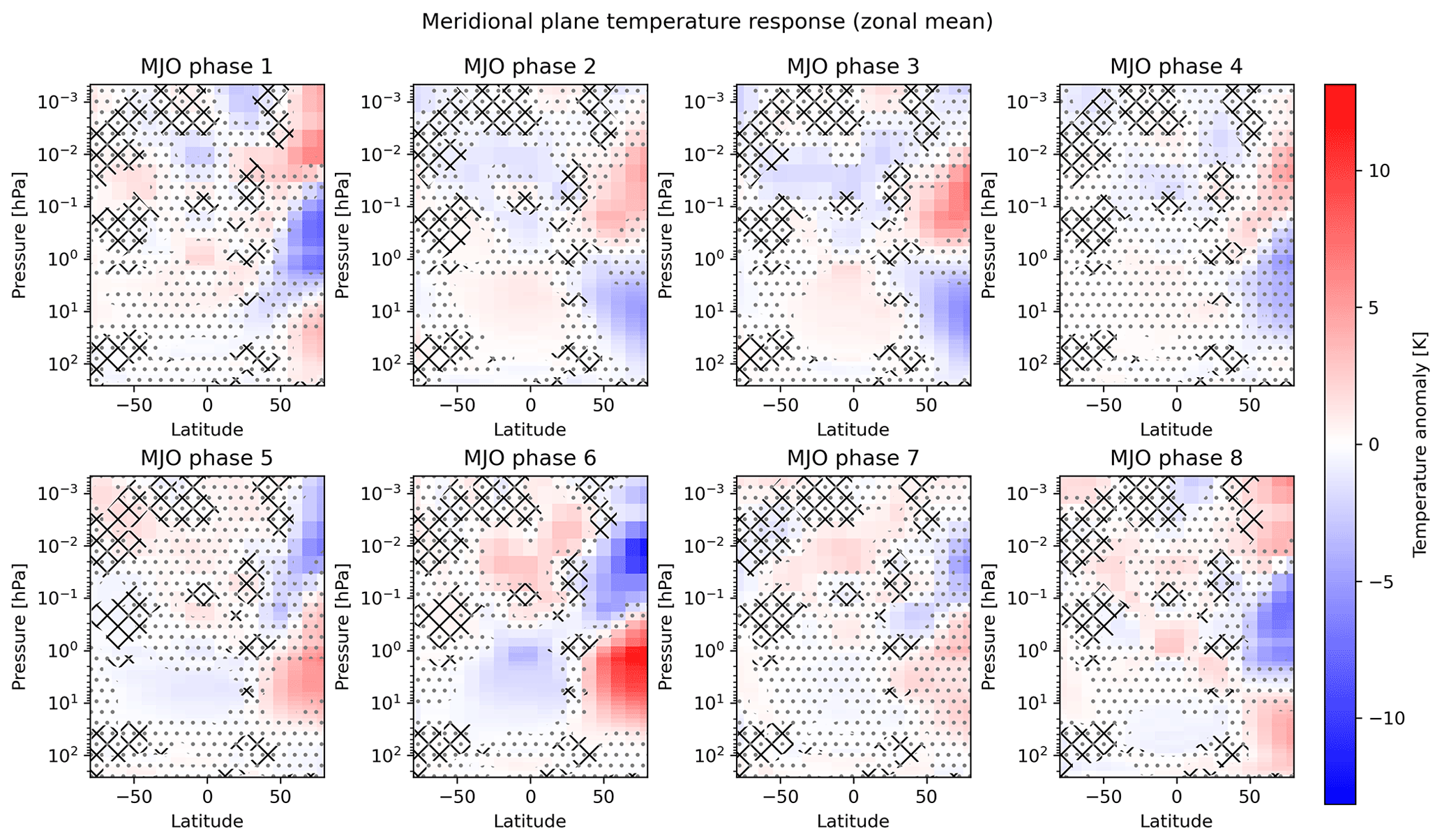
The transition of the five-zone signal between different MJO phases now emerges more clearly. At a simple level, two classes of the response pattern can be identified that correspond to both signs of the five-zone signal. The importance is the ordered appearance of these two classes: one class is coherently observed during the first half of the MJO cycle (particularly during phases 2 to 4, during which, e.g., the polar winter stratosphere is colder than normal), whereas the other class is seen for the second half of the MJO cycle (particularly during phases 5 to 7, during which, e.g., the polar winter stratosphere is warmer than normal). This coherent behavior further supports a real systematic response to the MJO being found here. The responses to phases 1 and 8 are somewhat more difficult to interpret since the polar winter anomaly dipole is extended by a third anomaly zone higher up. However, these phases can be systematically integrated in a more detailed recognition of the response transitions between the MJO phases as detailed in the following.

Looking more closely, a gradual change in the response from one MJO phase to the next within the two classes is seen in terms of a descent of the response pattern. This is most easily seen in the second half of the MJO cycle by starting with MJO phase 5 and following the cold anomalies in the boreal polar winter with one's eyes (blue area in the upper right of the MJO phase 5 panel in Fig. 4). The negative anomaly is at the highest altitudes there and then descends in the following MJO phases, including phase 8. Such behavior can also be roughly identified during the first half of the MJO cycle when starting in MJO phase 1 with the upper positive polar winter anomaly (red area in the upper right of the MJO phase 1 panel in Fig. 4) and following its vertical position towards phase 4. Note that the summer mesosphere extension of the five-zone signal remains at its altitude during all eight MJO phases.

Moreover, one could also combine the gradual changes within both classes into a roughly continuous descent during the course of a complete MJO cycle. This is most easily seen when starting again in phase 5, but this time with the positive stratospheric winter anomaly (red area on the right at about 5 hPa of the MJO phase 5 panel in Fig. 4). Although somewhat more irregular, this anomaly descends down to about 100 hPa in MJO phase 8. Now, the additionally appearing polar positive anomaly areas at the highest altitudes during phases 8 and 1 could be seen as replacements for the vanishing positive anomaly at the lowest altitudes. Then the descent could be continued in MJO phase 1 with the upper positive polar winter anomaly as before. Hence, the special responses of phases 8 and 1 would realize the transition from the one class of the response to the other class.

The only pronounced discontinuity of the transition appears between MJO phases 4 and 5, where the sign of the response is abruptly switched. Therefore, the response evolution could be interpreted in a way that it starts in phase 5, descends during the following MJO phases including 8 and 1 until the pattern looks reversed in its sign, and is then abruptly reset to its original state after MJO phase 4. However, one could also argue that this abrupt transition is just a statistical artifact, since the signal in MJO phase 4 is relatively weak and insignificant. This leaves room for the speculation that a smooth backward transition could actually be realized in reality and become visible with a longer dataset. This speculation is further underpinned by the following discussion of the austral winter situation (Sect. 3.3).

Note that we have used the boreal winter and QBO easterly situation to describe the two response pattern classes and the gradual transitions, since both are most clearly visible for this case. However, at least the two response classes and in outline also parts of the gradual transition can be seen for other atmospheric conditions.

We have also checked the MA temperature response for the boreal winter and QBO westerly situation (Fig. 5) and find that it is much less clear than in the previously described boreal winter and QBO easterly case. This meets the expectations, as will be further discussed in Sect. 4.5. Nevertheless, the five-zone signal is also recognizable for some of the MJO phases, particularly phases 5 and 7. Hence, the MJO signals in MA temperature might not have totally vanished, so that the corresponding structure might become clearer in the future when longer observational records are available.

Figure 5 Similar to Fig. 4 but for the boreal winter and austral summer and the QBO westerly situation. Note that the color scale is different compared to Fig. 4.

3.3 Austral winter and boreal summer

The analysis of the data restricted to austral winter (Fig. 6) shows generally that the previously described boreal winter signals can also be detected in the Southern Hemisphere, although they are weaker and patchier. The strongest anomalies are again found in the polar winter regions but have, with ±3 K, only half of the magnitude compared to the boreal winter data, which have not been filtered for the QBO (Fig. 2). The polar winter signal shows generally again the pattern of a vertical dipole, while individual exceptions with a third zone also exist here, e.g., for MJO phase 5. The equatorial vertical dipole is partly more difficult to identify but is still clearly visible for many MJO phases, at least for phases 3, 4, 6, 7 and 8. Also, the summer mesosphere extension, this time in the Northern Hemisphere of course, can be identified in the signal of most MJO phases, e.g., for MJO phase 6. However, the summer mesosphere signal is more complex for some of the MJO phases: it has a dipole structure itself (e.g., MJO phases 3 and 7). It is expected from the previous results that the summer mesospheric anomaly has the same sign as the upper part of the equatorial dipole, which is actually seen for these phases too. However, in addition, we find another anomaly zone above, which has the opposite sign, forming a summer mesospheric dipole. It is remarkable that this dipole also reverses sign for the opposing MJO phases 3 and 7, which indicates a real systematic behavior.

Figure 6 Similar to Fig. 2 but for the austral winter or boreal summer situation. Note that the color scale is different compared to Fig. 2.

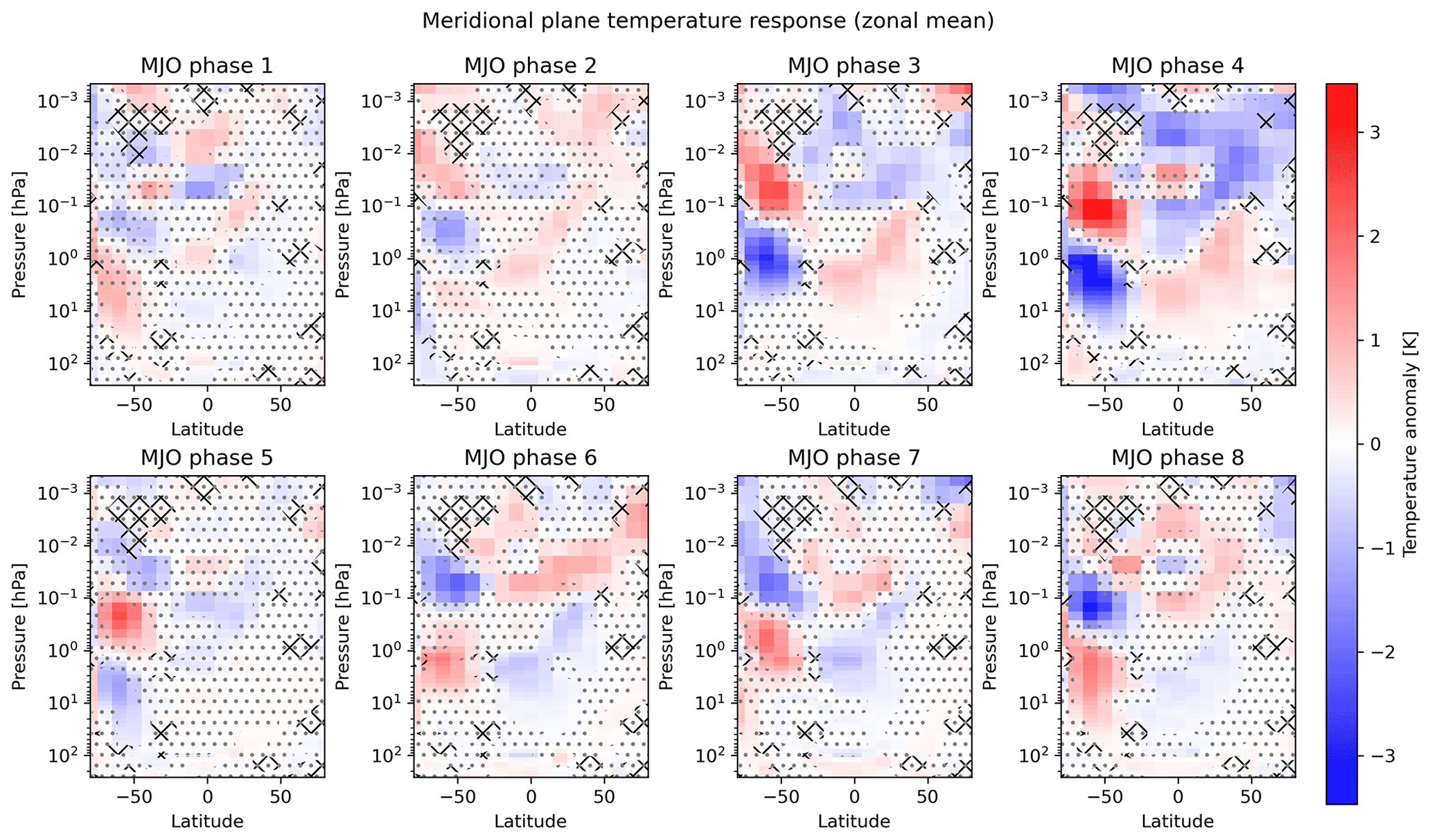
The two significance estimation approaches provide quite different results: the MCIP method shows less and smaller significant areas, which is connected to the generally weaker response. The MCS instead suggests a significant systematic response over all eight phases in almost all places of the meridional plane. Hence, although the responses are weak in terms of the individual temperature anomalies, they appear to be clearly systematically correlated with the eight MJO phases. This might be connected to the fact that this season is dynamically less disturbed, so that less interfering disturbances mask the pure MJO signal.

We note that it is not necessarily expected that the austral winter response is recognizable as a counterpart of the boreal winter response, and its existence appears noteworthy on its own. This is also because the austral winter hemisphere is usually dynamically much more quiescent than the boreal winter hemisphere. In particular, SSWs are very rare events in the Southern Hemisphere, and only two such warmings have been observed since routine observations started some decades ago, i.e., in the austral winters of 2002 and 2019 (e.g., Jucker et al., 2021; Allen et al., 2003; von Savigny et al., 2005). While the first one is not included in the MLS period anyway, we have repeated our analysis with the MLS dataset, restricted to the period before the end of 2018, so that the second warming is also not included (Fig. S2 in the Supplement). It turns out that the pattern of the temperature signal to the MJO phases remains basically unchanged when this warming is excluded. In contrast to expectations, the strongest anomalies are even a bit stronger without 2019. This shows that the appearance of SSWs is not a precondition for the MJO-induced temperature response pattern, a fact that was unclear from analyzing the boreal winter response alone. However, due to the different magnitudes of the responses, the results still indicate that the dynamical disturbances of the boreal winter hemisphere are important for an amplification of the MJO signal.

When comparing the boreal and austral winter five-zone signal (Figs. 2 and 6), it becomes evident that the sign of the response is identical for most individual MJO phases. This is particularly true when comparing the austral winter response to the boreal winter and QBO easterly situation (Figs. 4 and 6), which shows a higher level of structure as discussed before. Hence, the phasing of the signal with respect to the MJO trigger appears to be generally similar for both hemispheres.

Also, the phase transition shows similarities to the boreal winter (and QBO easterly) situation. Again, the two different signs of the pattern are seen and can again be attributed to the first and second halves, respectively, of the MJO cycle. Overall, one can also identify the gradual descent of the pattern from one MJO phase to the next. Again, one can start with MJO phase 5 and track the upper negative polar anomaly (blue region at 0.01 hPa on the left of the MJO phase 5 panel in Fig. 6). It descends down to about 0.1 hPa in phase 8 and then further across phase 1 down to 5 hPa in phase 4. Note that one could also start in MJO phase 2 by tracking the upper positive polar anomaly.

Interestingly, there is no clear indication of an abrupt backward transition. Instead, a third anomaly zone (negative) appears here in the responses of phases 4 and 5, which again suggests the interpretation as a smooth backward transition, similarly to the discussion of phases 1 and 8 in Sect. 3.2. Considering that this third (positive) anomaly zone in phase 8 also appears at least to some extent in the austral winter, one could suspect that the cycle of the temperature responses during the course of the MJO is actually closed in this case without any abrupt backward transition. This underpins the speculation that the alleged abrupt backward transition seen in the boreal winter and QBO easterly situation (Sect. 3.2) is actually a statistical artifact.

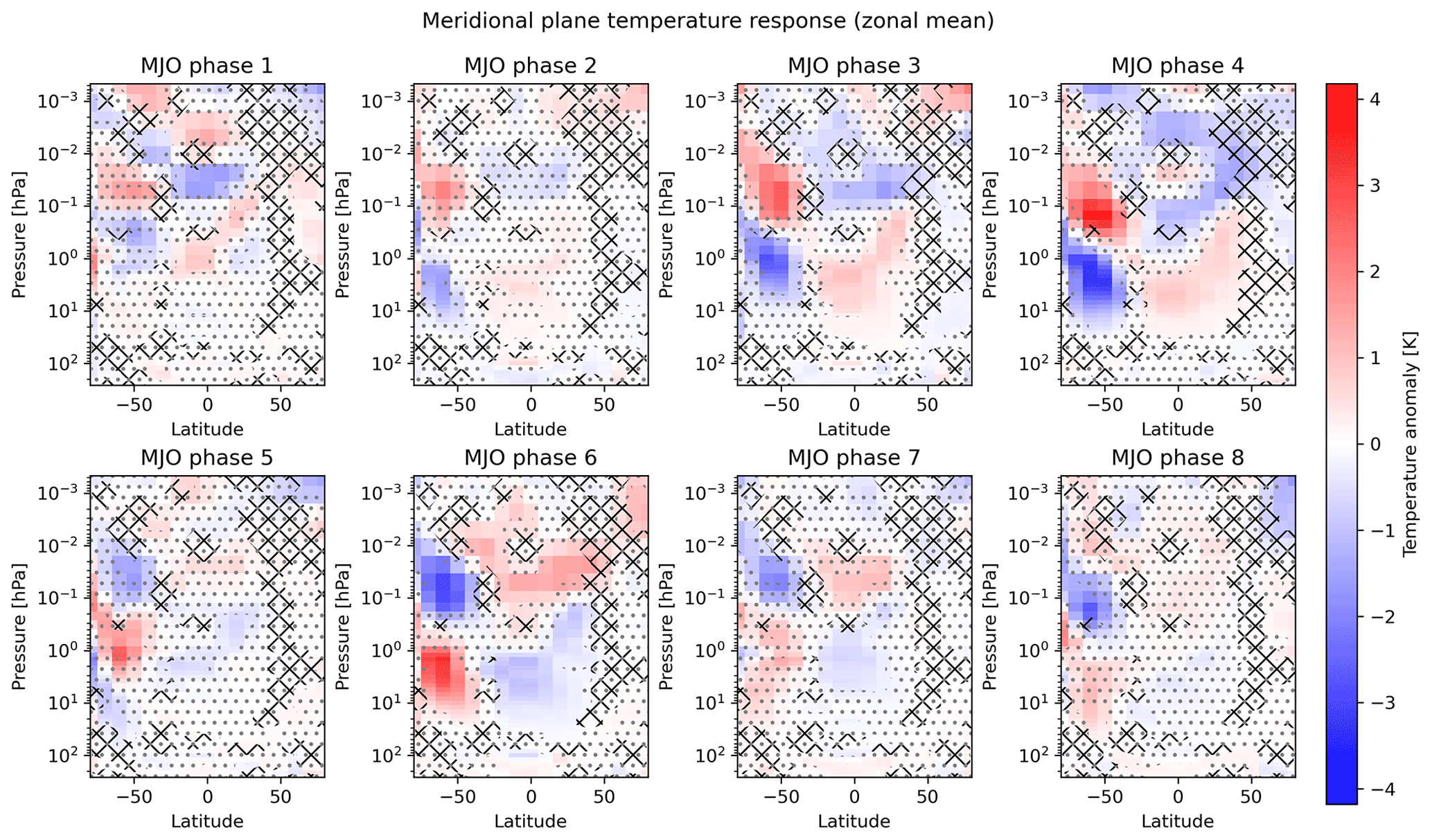
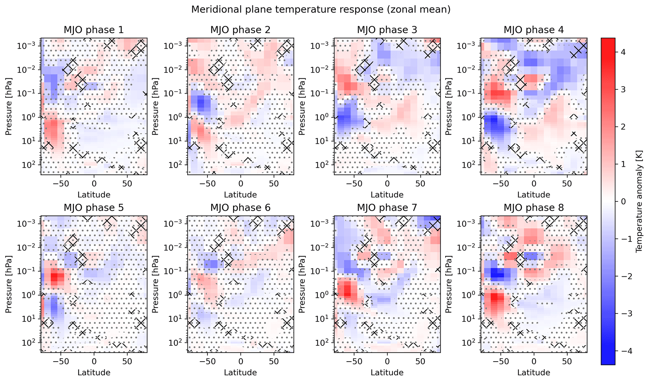
3.4 Austral winter and boreal summer and the state of the QBO

We have also checked the QBO influence for the austral winter situation and find that the QBO does not have such a big impact during this season, in contrast to the boreal winter situation described before. The results are shown in Fig. 7 for QBO easterly and Fig. 8 for QBO westerly. Although some differences between the MA temperature responses for QBO easterly and westerly are seen, they do not have a clear systematical structure, so that these differences could also be random effects due to the different sampling periods. The only noteworthy difference is that the austral winter and QBO easterly case (Fig. 7) does not show a clear descent of the pattern (nevertheless, the two classes and signs of the pattern corresponding to the first and second halves of the MJO cycle are still clearly visible), whereas this descent can be seen in outlines in the austral winter and QBO westerly case (Fig. 8).

Figure 7 Similar to Fig. 6 but for the austral winter and boreal summer and the QBO easterly situation. Note that the color scale is different compared to Fig. 6.

Figure 8 Similar to Fig. 6 but for the austral winter and boreal summer and the QBO westerly situation. Note that the color scale is different compared to Fig. 6.

3.5 No filtering for environmental conditions

It became obvious in the previous description that external conditions like the season and the QBO have a strong influence on the strength and spatial structure of the signal. Hence, analyzed data that comprise different states of these conditions can result in reduced signals due to interferences of the individual signals for different conditions. Therefore, we do not discuss the unfiltered analysis here in detail. Nevertheless, we show the results for the unfiltered data (only a filtering for an MJO strength of greater than 1 is applied) in the Supplement (Fig. S1) and note here that the derived temperature anomalies connected to the MJO signals are in this case in the range of ±2 K.

4 Discussion and relation of the results to previous research

It is a major aim of the present paper to communicate the finding of the five-zone signal in MA temperature in connection with the MJO as a broad overarching signal. To cover the broad picture, we included the complete meridional plane, all MJO phases and different seasons. To stay focused, the study intentionally has a purely statistical character, so that it does not determine causalities or physical mechanisms. Furthermore, it is mostly based on purely observational data. There are a number of previous studies in this area of research with partly overlapping aspects. These studies are typically less broad in the above sense but instead also cover the physical explanation approaches of the found patterns.

This section aims at briefly relating our results to the previous publications to use synergies in terms of two aspects: firstly, to provide a broader picture that integrates and interrelates the current and previous studies; and secondly, to put forward some possible physical explanation in terms of the responsible mechanisms for the statistical results presented before.

4.1 Similarity to interhemispheric coupling (IHC)

The five-zone signal looks qualitatively similar to the temperature pattern of a known dynamical feature of the MA, the IHC. The IHC was first described by Becker et al. (2004) and is basically a chain of dynamical disturbances, which starts with a deviation of the planetary wave (PW) drag in the winter stratosphere. By additionally also modifying the MA gravity wave propagation, the disturbance then spreads across the winter MA towards the summer mesopause region. These dynamical disturbances also cause temperature anomalies with a spatial structure that is generally comparable to the one found here. A mechanism for the IHC was already proposed in the first publications (Becker et al., 2004; Becker and Schmitz, 2003; Becker and Fritts, 2006) using model experiments and then detailed by Körnich and Becker (2010). Some aspects are still the subject of the scientific discussion and refinement as, e.g., in Yasui et al. (2021).

After its discovery, the existence of the IHC was further supported by satellite observations of, e.g., noctilucent clouds (Karlsson et al., 2007, 2009b) and simulations (Karlsson et al., 2009a). These simulations can be used for a quick quantitative comparison of the spatial structure with our results. This comparison reveals that the pattern indeed also fits well in terms of the pressure levels of the strongest deviations (compare, e.g., Fig. 6 for the time lag of 15 d in Karlsson et al., 2009a, with our Fig. 2 for MJO phase 5, which are the periods of the strongest responses in both studies). We see, however, much stronger magnitudes of the effect of about ±6 K for northern winter filtering and ±10 K for the northern winter and QBO easterly filtering instead of ±3 K in Karlsson et al. (2009a).

Karlsson et al. (2009a) further pointed out that the IHC temperature pattern can develop with both signs, depending on the sign of the initial planetary wave drag disturbance. This fits to the two classes of response, which we have seen for the first and second parts, respectively, of the MJO cycle. The first half fits generally to the “weaker wave drag scenario” in Karlsson et al. (2009a), whereas the second half fits to the “stronger wave drag scenario”.

As an interim conclusion, we state that the five-zone signal is probably identical to the already known IHC temperature pattern. Hence, the MA part of the formation mechanism of the five-zone signal is probably the known IHC mechanism.

One of the new aspects of the present study is that the emergence of the IHC pattern has now been linked statistically to the MJO phase evolution. This leads to the assumption that the MJO can indeed act as a trigger for the IHC, i.e., that it can physically cause the initial PW drag deviation in both directions. Previously, the IHC was studied mainly in the context of SSW events. The MJO as a trigger is different from SSWs in such a way that, firstly, the MJO evolves continuously, periodically and relatively smoothly compared to the event-like SSWs. Secondly, the MJO repeats itself on the shorter intraseasonal timescale. Hence, a connected new aspect of this study is the indication that the MA temperature adapts well up into the mesosphere continuously to tropospheric dynamical forcing changes on the MJO timescale via the IHC mechanism. A new question for the research on the IHC emerges from our observation that the pattern appears to descend during the course of the MJO. To our knowledge, an altitude–time dependence of the IHC temperature pattern has not been explicitly described or explained in the literature so far.

To further support our findings being closely connected to the IHC, we list some more aspects that are broadly consistent with IHC publications in the following. The first aspect is that we see a difference in the temperature signals between the two polar regions: while the polar anomaly dipole is directly located above the northern polar region during boreal winter (Fig. 2), it is shifted somewhat more towards the Equator for the austral winter situation (Fig. 6). Without going into the details of the analysis by Karlsson et al. (2007), a similar feature is seen in their results: one important indicator of the IHC is the blue area in the northern polar area in the top panel of their Fig. 2. The top panel resembles our boreal winter situation, and it is seen that the blue area is directly located above the winter pole. When considering the austral summer situation (their middle panel), the blue area is not located directly above the pole but instead is shifted northwards to about −50^∘ latitude, which is basically consistent with our results. The second aspect is that Yasui et al. (2021) also not only consider a vertical dipole as the temperature response above the winter pole, but also see a third anomaly zone above the mesopause, which has the same sign as the stratospheric anomaly. We have also repeatedly seen this in the responses of individual MJO phases, e.g., phase 8 for the boreal winter and QBO easterly situation (Fig. 4). The third aspect is that Yasui et al. (2021) partly show the summer mesospheric response of the IHC being itself a vertical dipole with a positive anomaly and a negative anomaly instead of only one zone for certain time lags. We have seen such a feature for the austral winter situation (Fig. 6).

4.2 The interconnection of IHC, SSWs and the MJO

With the present findings, a statistical triangular relation between IHC, SSW and the MJO becomes obvious. First, the IHC pattern is inherently connected to SSWs, since SSWs may produce or amplify the polar winter part of the IHC temperature pattern. Second, the occurrence of SSWs was linked to the evolution of the MJO phases by Garfinkel et al. (2012). As a new aspect, we have now introduced the third side of the triangle, as we have statistically linked the IHC directly to the MJO. Overall, it should be expected that the connections between all three features should be mutually consistent, which is briefly discussed in the following.

However, first of all, we would like to make an aside on SSWs being a potential disturbing factor for our analysis. The SEA method is designed to average out all variability that is not correlated with the MJO phase evolution, but the success of this elimination can be reduced by unrelated variability with comparatively large magnitudes. We find the strongest responses to the MJO in the Northern Hemisphere winter, i.e., exactly where SSWs produce their strong variability. Hence, the objection might be raised that this strong polar winter variability is actually uncorrelated with the MJO and is not sufficiently eliminated, so that the method produces false responses. While we can indeed not totally exclude the possibility that uncorrelated variability still influences the results, we have several indications that the strong polar signal is overall truly correlated with the MJO phases. The first one is the fact that the occurrence of SSWs has been found to be itself correlated with the MJO as mentioned before and as further discussed below. Hence, the results presented here could also be interpreted as supportive for this idea instead of being an artifact. Second, we have also found a similar pattern for the Southern Hemisphere polar winter, which is dynamically much more quiescent, and periods without SSWs can be analyzed (Sect. 3.3). Third, one could also consider repeating the analysis for boreal winters only without SSW periods. We have quickly checked this approach, which indicated that the signature is still clearly visible. However, the number of days that go into the analysis is quite low when applying this additional filter, so that the interpretation needs particular care and has not been included here.

We have mentioned above (e.g., Sect. 3.2) that the MA temperature responses can be roughly divided into two classes with opposite signs. The responses, which roughly belong to the second half of the MJO cycle (phases 5 to 8), show a warm polar winter stratosphere and can therefore be related to the SSW case. Garfinkel et al. (2012) find MJO phase 7 to be the dominating phase directly preceding SSWs (time lag of 1 to 12 d), so that the phasing is broadly consistent with our results. However, from our analyses, one would have concluded that MJO phases 5 and 6 show the strongest SSW-like responses (compare Figs. 2 and 4), which might look like a discrepancy. However, the pattern in our analysis descends from phase 5 to phase 8 at least for the boreal winter and QBO easterly case, so that we see a continuous evolution of the pattern. Garfinkel et al. (2012) instead use a sharp SSW detection criterion, which is based on the atmospheric state at 10 hPa. This is at the lower bound of the polar positive temperature anomaly found here for MJO phases 5 and 6 but is more central in the positive anomaly for phase 7. Hence, what we already identify as an SSW-like pattern in phases 5 and 6 might, with regard to the exact altitudes, be a precursor of the SSW-like pattern considered by Garfinkel et al. (2012), which is then only reached in phase 7. This would also be roughly consistent with the result of Garfinkel et al. (2012) that MJO phase 6 is a precursor of SSWs with a longer time lag of 13 to 24 d. We note that the comparison is only a rough qualitative cross-check since the analyses differ in their setups and are always complicated by the inherent large variability.

We note as a byproduct of the discussion that the descent of the IHC pattern, which has been shown in the present analysis, might also be relevant for other comparisons and considerations in this area of research, similar to the example above.

Overall, we consider the general consistency with Garfinkel et al. (2012) to be important support for the hypothesis that the statistical relationship between the MJO and the IHC brought up in this study is a real effect and not a statistical artifact.

4.3 MJO–IHC linkage: potential coupling by planetary wave forcing

The joint reason for SSW and IHC occurrences is known to be a deviation in the PW forcing of the winter stratosphere. The sign of the IHC pattern depends on the sign of the PW drag deviation, called strong or weak planetary wave forcing, respectively. Our findings now indicate a relation of the MJO and such PW drag deviations relevant to the IHC. Although not proven by our statistical approach, the MJO appears to act as a source of the initial PW disturbances, which can weaken (MJO phases 1 to 4) and strengthen (MJO phases 5 to 8) the relevant PW activity in the winter stratosphere.

It is therefore of interest to consider the study by Wang et al. (2018a), which explores the effect of MJO phase occurrences on wave activity in the Northern Hemisphere winter stratosphere. Wang et al. (2018a) find that a higher occurrence frequency of MJO phase 4 is in line with weaker wave activity. This is roughly consistent with our findings in the sense that MJO phase 4 belongs to the first half of the MJO cycle. Furthermore, Wang et al. (2018a) find higher wave activity for MJO phase 7, which is also roughly consistent with our findings.

The reason for the PW drag modulation is, according to Wang et al. (2018a), that MJO wave activity is in antiphase with the climatologically apparent waves in the respective region for MJO phase 4 and in phase for MJO phase 7. Hence, a mechanism for the relationship between the tropospheric MJO and the MA IHC pattern found in our study should probably consider such PW wave interferences as a link.

However, our results also raise new questions in this context: Wang et al. (2018a) state that all other MJO phases should not have a strong influence on the extratropical stratosphere, because there is no clear in-phase or antiphase relationship of the MJO-related waves and the climatological waves. We find instead a response throughout the middle atmosphere for all the MJO phases. This could be consistent as long as the MA responses to all the other MJO phases are considered time-lagged results of the forcings of only MJO phases 4 and 7. However, it is then surprising that the main forcing occurs towards the end of those consecutive MJO phases, which show the appropriate sign of the response (phases 1 to 4 and 5 to 8, respectively).

4.4 Comparison with previous studies covering the relationship of the MJO and MA temperature

There are some studies already dealing with the MJO–MA temperature relationship for particular MJO phases independent of IHC, which can be compared to our results. We note, however, that strict comparisons are difficult, not only because of the partly high variability of MA temperature, different analysis setups and different datasets, but also because many studies analyze the state of the MA as a function of relatively long time lags after only selected MJO phases. Our analysis works without time lags and instead considers all eight MJO phases to uncover the gradual changes in the responses between the individual MJO phases. Hence, the comparisons mostly have a qualitative character.

The order of magnitude of the MJO-related temperature anomaly shown in Sun et al. (2021) is with ±5 K comparable to our analysis, as is the fact that the strongest anomalies are observed when the polar stratosphere shows the warm anomaly. The agreement of the orders of magnitude is particularly remarkable, since the periods of strongest variability are missing due to the exclusion of SSWs in Sun et al. (2021). Also, the order of magnitude of the temperature response reported in Yang et al. (2019) is comparable to our results of the boreal winter situation without QBO filtering (Fig. 2), i.e., in the situation for which the analysis setups are closest to each other.

The northern winter polar vertical dipole of the five-zone signal is, e.g., confirmed by Sun et al. (2021, Fig. 2). They also show the temporal switch in the dipole's sign, here between time lags 25 and 30 d after MJO phase 4. A consistent sign change in the temperature anomaly is also found in Yang et al. (2019, Fig. 1a) for a time lag of 0 d. It is seen that the stratospheric response is negative for MJO phases 2 and 3 and positive for phases 5 and 6, as in our study.

With respect to the timing, Sun et al. (2021) report a cooling of the Northern Hemisphere mesosphere 35 d after MJO phase 4. Yang et al. (2019) report a corresponding stratospheric warming after MJO phase 4 with a time lag of 30 d. Although both might still fit the appearance of this pattern in the second half of the MJO cycle in our data, we would have expected it earlier in terms of time lags after phase 4.

The results for the austral winter can be compared to Yang et al. (2017, Fig. 2a and b). They find cold anomalies at 10 hPa and a time lag of 0 d roughly for MJO phases 1 to 3 and warm anomalies for phases 5 to 7. We see the corresponding responses slightly shifted to MJO phases 2 to 4 and 6 to 8, respectively, and also somewhat different in altitude, but a rough consistency can be stated. A comparison of the complete meridional plane response for MJO phase 5, which is included in Yang et al. (2017, Fig. 4), also reveals a general consistency with our results. In particular, the results for the time lag of 10 d compare well to our MJO phase 6 response. Also, our magnitude of the anomalies fits roughly to the results of Yang et al. (2017).

4.5 Influence of the QBO on the MA temperature response to the MJO

For the influence of the QBO on the MJO–MA connection (e.g., Sect. 3.2), at least two possible types of interference have to be considered: the influence of the QBO on the MJO itself as well as the influence of the QBO, within the stratosphere, on high-latitude stratospheric dynamics.

4.5.1 Influence of the QBO on the MJO

The influence of the QBO on the MJO is currently an active field of research and is still debated (e.g., Yoo and Son, 2016; Zhang and Zhang, 2018; Wang and Wang, 2021). Overall, there appears to be a strengthening of MJO effects for the QBO easterly phase during boreal winter, which fits qualitatively very well to our findings. Note that, combined with our results, this would be a net effect of the tropical lower stratosphere on the complete MA conveyed by the troposphere, where the MJO is active.

Regarding the seasonal differences, the QBO influence on the MJO has mainly been reported for boreal winter (e.g., Yoo and Son, 2016; Son et al., 2017). However, using two more sophisticated analysis approaches (QBO determination and the BSISO index), Densmore et al. (2019) claim that there is also an QBO–MJO relationship during boreal summer, which is reversed compared to boreal winter. Our examination of the QBO influence on the MJO–MA connection during boreal summer (Sect. 3.4 and Figs. 7 and 8) showed no clear indication of a QBO influence during boreal summer.

4.5.2 Influence of the QBO on the polar stratosphere

The second possible type of interference is the influence, within the stratosphere, of the equatorial QBO on the polar winter stratosphere (e.g., Holton and Tan, 1980), which results in the polar winter stratosphere tending to be colder during the QBO westerly phase and warmer during the QBO easterly phase (e.g., Labitzke and van Loon, 1992). This observation is connected to a known influence of the QBO on the occurrence of SSWs during boreal winter (e.g., Camp and Tung, 2007). Hence, both the QBO and the MJO have an influence on the occurrence on SSWs, which have a large influence on the polar MA temperature. Therefore, one reason for the finding that the QBO apparently changes the MJO's influence on MA temperature could be that both influence the occurrence of the SSWs simultaneously, with possible interactions or interferences of the effects.

Note that this QBO effect would not necessarily remain restricted to the polar winter stratosphere. Instead, it has already been shown that the QBO influence on this region also influences other regions of the MA via the IHC mechanism (Espy et al., 2011). Moreover, Murphy et al. (2012) show that some details of the IHC mechanism are themselves modified by the QBO phase. Hence, it is plausible that the temperature response to the MJO, which is conveyed by the IHC mechanism, is subject to this QBO influence in the complete MA.

4.5.3 Concluding remarks on the QBO influence

Overall, we cannot discriminate the relative importance of the two possible types of the QBO influence on the MA temperature signal to the MJO. While a consistency of major aspects can be seen for the QBO influence on the MJO itself (Sect. 4.5.1), we cannot draw any reliable conclusions about the importance of the inner-stratospheric influence (Sect. 4.5.2). This might be possible in the future, when longer datasets allow for a more detailed filtering with respect to other environmental parameters, particularly the exclusion of SSWs.

There is obviously a hemispheric asymmetry of the QBO influence on the MA temperature response to the MJO (Sect. 3.2 and 3.4). One possible explanation for this apparent asymmetry could be the generally higher variability of the Northern Hemisphere boreal winter situation. This might require a particularly strong MJO signal to dominate the intraseasonal variability in the Northern Hemisphere. In addition, the influence of the QBO easterly phase on the MJO during boreal winter could be a major factor in facilitating this strong MJO signal during this season. In contrast, a weaker MJO might already be able to dominate the signal in the more quiescent Southern Hemisphere, so that a QBO support is not needed to produce the austral winter signal. Another explanation could be the mentioned modification of the occurrence rates of SSWs by the QBO, which is only relevant during boreal winter, because SSWs only rarely happen at all in the Southern Hemisphere.

4.6 Limitations of the presented analysis

To obtain a complete picture, it will be necessary to study the MJO influence on the MA temperature, also with respect to additional environmental conditions, at least for the state of the El Niño–Southern Oscillation (ENSO) and the solar 11-year cycle. The length of the analyzed datasets currently limits the number of filters, which can be simultaneously applied, so that we have focused on those influences, which we expected to be most important based on previous research. However, the discrimination of the QBO states in particular based on comparatively only a few years of data might be affected by, e.g., the underlying state of the 11-year cycle. Also, a precise discrimination of boreal winters with and without SSWs is of interest but also requires a longer dataset.

Furthermore, we emphasize again the statistical nature of our analysis, which cannot examine the causality and possible physical mechanisms. The present publication aims at making the revealed statistical indications of a connection of the MJO and the IHC already available to the community in order to foster research on the underlying mechanisms. However, to prevent the publication of possible statistical artifacts or spurious correlations, we have embedded our results in previous research, which shows the overall plausibility of a real effect, for which the physical reason can be established in the future.

We note that the statistical approach does not determine the direction of a physical influence either. From the previous literature, it appears plausible that an influence at least in the direction from the tropospheric MJO on the MA temperature via an alteration of the wave driving exists. However, possible influences in the opposite direction or feedback loops are not excluded by our study.

5 Summary and conclusions

We have statistically analyzed the connection of the MJO and the MA temperature based purely on observations of MA temperature. We have included all MJO phases in the analysis and have distinguished different seasons and states of the QBO.

We have indeed found that the MA temperature is influenced in a statistical sense by the state of the MJO in large areas of the MA and under roughly all considered atmospheric conditions. Still, the strength of the signal varies considerably with both the atmospheric conditions and the region of the MA.

Most notably, a pronounced characteristic response pattern, which we called here temporarily the “five-zone signal”, manifested itself under many atmospheric conditions. The first two zones (compare Fig. 3) are two anomaly areas with opposing signs in the polar winter stratosphere and mesosphere, together constituting a dipole response above the winter pole. These zones mostly show the strongest anomalies among all five zones. A second dipole, comprising the third and fourth zones, is found in the equatorial stratosphere and mesosphere. This dipole has a reversed sign compared to the polar winter dipole. The fifth zone is found above the summer pole in the mesopause region, so that the five-zone signal spans almost the complete meridional plane. The anomaly of the fifth zone has the same sign as the equatorial mesospheric zone. The overall sign of the complete five-zone signal is different for different MJO phases. It has been checked with two Monte Carlo approaches that the anomalies of at least these five zones are broadly significant for most analyzed cases.

A pattern like the five-zone signal is known in MA research from a feature called interhemispheric coupling (IHC). This IHC mechanism basically describes how an initial disturbance in planetary wave drag in the winter stratosphere propagates due to a chain of different dynamical effects through the MA and thereby causes a similar pattern of temperature disturbances as we have seen here for the MJO signals. Moreover, the IHC mechanism works for weak and strong planetary wave activity, causing the one or the other sign of the temperature anomaly pattern as we found here for different MJO phases.

Hence, one major outcome of the present observational and statistical analysis is the idea that the MJO can trigger the IHC pattern in MA temperature. The present study therefore statistically connects an atmospheric feature mostly known in tropospheric research, the MJO, with one mostly known in MA research, the IHC. The MJO as a further potential trigger of the IHC brings new aspects to research on MA dynamics, since its timescale and periodicity characteristics are quite different from SSWs, which have so far been considered as the starting point in IHC studies.

The analysis, applied individually to boreal or austral winter data, has revealed that the five-zone signal appears in both hemispheres, with the pattern being roughly mirrored at the Equator. The boreal winter signal is, however, much stronger. Furthermore, the signal during the boreal winter season also shows a strong dependence on the QBO phase, which we have not convincingly seen for the austral winter. Overall, the strongest anomalies and the clearest spatial patterns appear for the boreal winter combined with the QBO easterly phase. In this case, we have found temperature anomalies in the range of ±10 K, with the strongest anomalies being located over the winter pole. For the austral winter the anomalies are, with ±3 K, much smaller, but nevertheless the spatial pattern can easily be identified for most MJO phases.

We also analyzed the change in the MA temperature signals, while the MJO transitions through its eight phases. For most atmospheric conditions, we could identify a systematic behavior, which is again most clear for boreal winter and QBO easterly conditions. It can be described in two steps. First, the responses to the eight phases can mostly be attributed to either a “weak wave driving” or a “strong wave driving” class according to the sign of the five-zone signal. Second, for many transitions, one MJO phase to the next gradual descent of the five-zone signal to lower altitudes can be observed, suggesting that the MA reacts systematically to each of the MJO phases.

Although descending patterns are well known in the polar winter stratosphere, we are not aware of any discussion of a descending temperature anomaly pattern, which is explicitly related to the IHC or the MJO signals in MA temperature. Although large parts of the mechanism behind the descent can probably be explained by already available knowledge, it appears of interest to clarify in the future whether each phase of the MJO is able to trigger the IHC pattern at a different altitude or whether the IHC pattern inherently descends after it has been triggered once by a certain MJO phase or a combination of both.

The results presented here have a statistical character and therefore do not guarantee a real causal connection or uncover the physical mechanism. In particular, we do not state that a certain MJO phase is the causal reason for the MA temperature pattern, which we obtain for that phase. Since propagation speeds have to be considered in a physical mechanism, it seems more likely that a pattern seen for one MJO phase has been triggered by previous MJO phases. However, by embedding our results in the context of previous research, we have made plausible that a real causal connection as an underlying reason can be assumed.

Establishing an overall mechanism appears to require more extensive future research. Such a mechanism should, in our view, cover at least the following aspects: the nature of the generation of the initial wave disturbance by all the MJO phases, the propagation of the signal in both hemispheres as well as in summer and winter, the propagation in the winter hemisphere with and without SSWs, the interaction with the QBO and the descent of the IHC temperature pattern, while MJO evolves. Of particular interest would be a detailed temporal view of the propagation of the disturbances in the MA that explains which of the foregoing MJO phases are actually causally responsible for the MA temperature pattern that emerges statistically for a particular MJO phase in our results.

Given that our statistical findings are physically substantiated in the future, we think that the described influence of the MJO on MA temperature is a noteworthy example of the complex couplings across different atmospheric layers and geographical regions in the atmosphere. Because of the wide coverage of atmospheric regions and the included dynamical features, the observational results presented here can be a good benchmark of the representation of atmospheric couplings in atmospheric models, particularly in the context of intraseasonal weather predictions.