Volatile organic compound fluxes in the agricultural San Joaquin Valley – spatial distribution, source attribution, and inventory comparison

The San Joaquin Valley is an agricultural region in California that suffers from poor air quality. Since traffic emissions are decreasing, other sources of volatile organic compounds (VOCs) are gaining importance in the formation of secondary air pollutants. Using airborne eddy covariance, we conducted direct, spatially resolved flux observations of a wide range of VOCs in the San Joaquin Valley during June 2021 at 23–36 ^∘C. Through land-cover-informed footprint disaggregation, we were able to attribute emissions to sources and identify tracers for distinct source types. VOC mass fluxes were dominated by alcohols, mainly from dairy farms, while oak isoprene and citrus monoterpenes were important sources of reactivity. Comparisons with two commonly used inventories showed that isoprene emissions in the croplands were overestimated, while dairy and highway VOC emissions were generally underestimated in the inventories, and important citrus and biofuel VOC point sources were missing from the inventories. This study thus presents unprecedented insights into the VOC sources in an intensive agricultural region and provides much needed information for the improvement of inventories, air quality predictions, and regulations.

1 Introduction

The San Joaquin Valley in California is one of the regions with the worst air quality in the United States (US EPA and American Lung Association, 2022). Despite decades-long ozone control measures, the National Ambient Air Quality Standard of 70 ppb is frequently exceeded, especially in the summer (Faloona et al., 2020). High ozone contributes to cardiovascular and respiratory health risks and damages crops and ecosystems. Volatile organic compounds (VOCs), emitted by anthropogenic and biogenic sources, fuel ozone formation when nitrogen oxides (NO_x) are present.

The San Joaquin Valley is an intense agricultural production region, home to millions of cattle and dairy cows, and it is the leading US producer of many types of fruits and nuts (California Department of Food and Agriculture, 2020). It is also an important transportation corridor connecting southern and northern California and is home to 4.3 million people, the largest urban areas being Fresno and Bakersfield (Public Policy Institute of California, 2018). Moreover, there are ca. 47 000 active oil and gas wells in the San Joaquin Valley (CALGEM, 2022). Agriculture including dairy and cattle farms (Gentner et al., 2014a, b; Hu et al., 2012; Marklein et al., 2021; Shaw et al., 2007; Malkina et al., 2011), natural landscapes (Misztal et al., 2014), urban areas, transportation (Hu et al., 2012), and oil and gas production (Gentner et al., 2014a) are known VOC sources in the San Joaquin Valley.

With reductions in Californian transportation VOC emissions over the last few decades (Warneke et al., 2012), the relative importance of other emission sources contributing to poor air quality is increasing. Based on air quality modeling, Hu et al. (2012) therefore predicted that livestock feed and mobile-source VOC emissions would contribute almost equally to ozone production in the San Joaquin Valley by 2020. However, the VOC sources in the San Joaquin Valley and their emission strengths are not well understood. For example, Pusede et al. (2015) found that unidentified molecules contributed significantly to ozone production in the San Joaquin Valley, especially at high temperatures. A comparison with aircraft observations showed that a regional air quality model underestimated ozone near dairy farms and oil fields (Cai et al., 2016).

Atmospheric chemistry models used to forecast air quality and guide policy decisions are built on emission inventories. Such inventories are typically based on bottom-up reporting or top-down inference of emissions from concentration measurements using chemical transport models. These strategies all have significant uncertainties since they are indirect. Direct, spatially resolved flux observations enable direct validation of emission inventories. Airborne eddy covariance measurements of VOCs have previously been used to validate inventories in an urban area (Vaughan et al., 2017) and in Californian oak forests (Misztal et al., 2016). A previous airborne VOC flux study covering parts of the San Joaquin Valley region (Misztal et al., 2014, 2016; Karl et al., 2013) was limited to few VOCs, since the available measurement technique (proton transfer reaction quadrupole mass spectrometry, PTR-quadrupole-MS) did not enable the simultaneous observation of many species at the high time resolution necessary for airborne eddy covariance. State-of-the-art instrumentation (PTR-ToF-MS; ToF denotes time of flight) has dramatically increased the number of compounds observable at the same time (Blake et al., 2004; Krechmer et al., 2018).

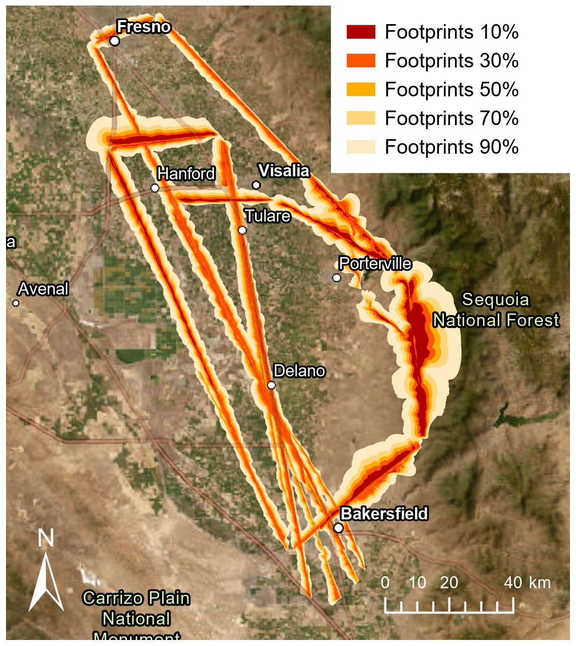
Figure 1 Footprints along the flight tracks for each observed flux measurement during the campaign (therefore, overlaps exist). The different colors show the areas where the 10th, 30th, 50th, 70th, and 90th percentiles of the measured fluxes originated. Footprints were derived from the KL04+ model. Map: TerraColor imagery via Esri ArcGIS Pro.

In this work, we apply direct observations of spatially resolved emission and deposition fluxes of a wide range of VOCs using airborne eddy covariance. Spatial comparisons help in the identification of inventory biases associated with regionally specific emission sources. We also provide estimates of source emission strengths by footprint disaggregation (Hutjes et al., 2010), a method which has not previously been applied to VOC fluxes. Thus, this work seeks to identify and quantify relevant VOC emission sources in the San Joaquin Valley and their contribution to ozone formation, and it validates two commonly used emission inventories with direct observations.

2 Methods

2.1 Flight routes, study region, and meteorological conditions

As part of the RECAP-CA (Re-Evaluating the Chemistry of Air Pollutants in California) campaign, seven flights were conducted over the San Joaquin Valley between 1 and 22 June 2021. Routes were selected to ensure a good coverage of important VOC sources in the southern San Joaquin Valley, including dairy farms, the I-99 highway, oil and gas fields northeast of Bakersfield, urban areas, and oak woodlands in the Sierra Nevada foothills. Each of the seven 5 h long flights was conducted on a different day and along the same flight tracks (Fig. 1). Every other flight included a 12–15 km long stacked racetrack pattern (Karl et al., 2013) flown at four to six altitudes evenly spaced between ∼300 m and the top of the planetary boundary layer (PBL), the local height of which was determined by a sounding preceding the racetrack pattern. The flights containing stacked racetracks were cut short at the northern end, while the others reached up to Fresno. The flight altitude was kept stable at 300–400 m a.g.l. (above ground level), since low, stable altitude and long legs assure good-quality airborne flux measurements (Karl et al., 2013). The aircraft flew slowly at an airspeed of 50–60 m s⁻¹ to ensure a high spatial resolution.

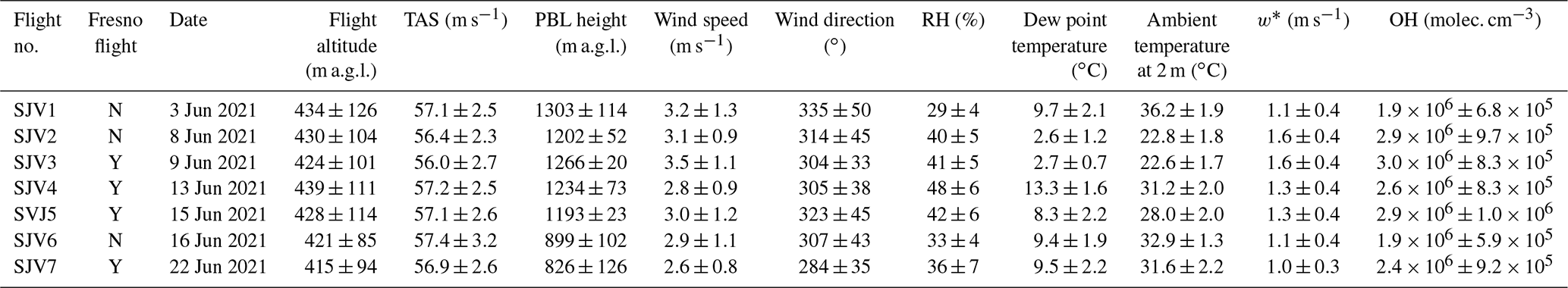
Table 1 provides an overview of the meteorological variables for each flight. Average ambient temperatures at 2 m a.g.l. ranged from 23 to 36 ^∘C. There was no precipitation. PBL heights were 800–1000 m a.g.l. Flight days and routes were chosen so that no cloud cover was encountered. The flights were performed between 11:00 and 17:00 LT (local time) to ensure homogeneous turbulent conditions and a high PBL.

Table 1 Average (± standard deviation) for meteorological variables and modeled OH for each flight. RH: relative humidity, TAS: true air speed. w^*: Deardorff velocity (convective velocity scale). “a.g.l.”: above ground level. “Fresno flight” indicates whether a flight included Fresno in the north (Y). If it did not (N), stacked racetrack patterns were flown at a suitable location in order to measure vertical flux gradients.

2.2 Aircraft

A two-engine UV-18A Twin Otter research aircraft was operated by the Naval Postgraduate School out of Hollywood Burbank Airport, CA. The aircraft is equipped with micrometeorological sensors and is capable of flux measurements (Karl et al., 2013). The Naval Postgraduate School (NPS) Twin Otter payload during RECAP-CA included total temperature measured by a Rosemount probe; dew point temperature (chilled mirror, EdgeTech Inc., USA); barometric, dynamic, and radome-angle pressures based on barometric and differential transducers (Setra Systems Inc., USA); total air speed; mean wind, slip, and attack angles measured by a radome flow angle probe; GPS pitch, roll, and heading (TANS Vector platform attitude, Trimble Inc., USA); GPS latitude, longitude, altitude, ground speed, and track (NovAtel, Inc., USA); and latitude, longitude, altitude, ground speed and track, pitch, roll, and heading measured by C-MIGITS III (GPS/INS, Systron Inc., Canada).

Air was drawn from a 7.62 cm isokinetic pipe inlet extending above the nose of the plane. Ambient air gets diffused from a 5.2 cm (inner diameter) orifice at the tip (area ratio of about 2) to another diffuser with an area ratio of 5, resulting in a flow speed inside the tube of about 10 % of the aircraft speed. Vertical wind speed was measured by a five-hole radome probe with 33^∘ half angles at the nose of the aircraft. Corrections based on “Lenschow maneuvers” (Lenschow, 1986) were applied to ensure that the vertical wind speed is unaffected by the aircraft movement and flow distortion at the nose. More detailed descriptions of this particular aircraft can be found in Hegg et al. (2005).

2.3 VOC measurements

2.3.1 Sampling and instrument operation

Ambient air was sampled via a 90 cm long heated (40 ^∘C) $\mathrm{1}/\mathrm{4}$ in. Teflon line through a Teflon filter from the abovementioned isokinetic inlet (flow speed ca. 6 m s⁻¹ for 5 m length) with a mass flow controller at 1.5 L min⁻¹. The resulting lag time between the wind sensor and VOC detection was around 3 s.

The Vocus proton transfer reaction time-of-flight mass spectrometry (Vocus PTR-ToF-MS, Aerodyne Research Inc., Billerica, MA, USA; Krechmer et al., 2018) instrument was operated at 2.0 mbar reactor pressure, 60 ^∘C reactor temperature, a potential gradient along the focusing ion–molecule reactor (FIMR) of 590 V, and a resulting $E/N$ of ca. 130 Td. This $E/N$ is expected to cause only moderate fragmentation (Yuan et al., 2017b). Unlike with traditional PTR-MS instruments, in the Vocus instrument the fragmentation rate is strongly (often more strongly than by $E/N$) affected by the gradient between skimmer 1 and skimmer 2 (or between skimmer 1 and big-segmented-quadrupole (BSQ) front voltage) (Coggon et al., 2023). The difference between skimmer 1 and skimmer 2 was changed once during the campaign from 6 to 9.1 V, which resulted in an improved sensitivity for some VOCs (e.g., methanol, which is prone to water clustering) but stronger fragmentation for others (e.g., monoterpenes, sesquiterpenes, and nonanal), both of which effects were accounted for through calibration. The mass resolution was $\approx \mathrm{4800}\pm \mathrm{280}$ (average ± standard deviation). The reagent water flow was 20 sccm, resulting in a high water mixing ratio (10 % $v/v$–20 % $v/v$) in the FIMR, so the instrument showed no humidity dependence in its sensitivity. This is an advantage in flux measurements because it eliminates the necessity to correct for humidity differences between different eddies caused by water fluxes. The high water mixing ratio causes a large primary ion (H₃O⁺) signal, which is lowered by a BSQ that reduces the transmission of low-mass ions in order not to wear down the detector too quickly. However, we kept the voltage of the BSQ relatively low at 200 V so that low-mass VOCs like methanol could be detected with reasonable sensitivity. The methanol sensitivity was on average 58 cps ppb⁻¹ for the setting of low skimmer voltage difference and 136 cps ppb⁻¹ for the setting of high skimmer voltage difference.

Mass spectra were recorded for a mass range of 10–500 Da at 10 Hz time resolution (or 2 Hz time resolution for one flight out of seven: SJV6). Several times during each flight, zero-air measurements were conducted for 1–5 min, during direction changes of the aircraft, because data acquired during turns cannot be used for flux calculations. Circa two times during each flight, the zero-air measurement was followed by a pulse of calibration gas of ca. 1–5 min length. These calibration data were used to confirm that the instrument sensitivity after correction for the zero-air background did not change significantly with the lower inlet pressure at our flight altitude and that, consequently, the calibration factors acquired on the ground were applicable to the airborne data.

2.3.2 VOC data treatment and calibration

Raw PTR-ToF-MS data were processed using Tofware 3.2.3. At this stage, no dead-time correction was applied. A total of 630 peaks were chosen for peak fitting. Interpolated ion counts from zero-air measurements taken in flight were subtracted from the ambient data. The instrument zero at flight altitude was different from the zero on the ground due to pressure effects that changed the pressure control valve position. According to laboratory testing of pressure effects, the sensitivities at the heights we flew at were the same as on the ground after subtracting the flight zero. Throughout the campaign, one of three distinct gravimetrically manufactured multicomponent VOC standards (Apel-Riemer Environmental Inc., Colorado, USA) was used for ground calibrations every 1–3 d. Gas-standard-calibrated compounds are labeled in Table S1 in the Supplement. For most VOCs, the sensitivities were stable within 25 % over the campaign. For all $m/z$ values without a corresponding gas standard, the sensitivities were derived from a theoretical calibration, using a root function (the expected function of a ToF transmission) fitted to reaction-rate-normalized sensitivities of non-fragmenting and non-clustering gas-standard-calibrated VOCs (Holzinger et al., 2019; Jensen et al., 2023). This approach accounts for transmission effects dependent on $m/z$. The uncertainties in this and the gas-standard calibration are based on typical estimates for the uncertainty in the theoretical calibration (50 %) and the gas-standard calibration uncertainty (20 %), which consists of the calibration standard uncertainty and the uncertainty in the mass flow controller. The resulting estimated uncertainty in the calibration for gas-standard-calibrated VOCs was 20 %, while it was 54 % for all other VOCs (propagated from 20 % and 50 %).

2.3.3 VOC identification from mass spectra

The PTR-ToF-MS method provides exact masses that can be linked to chemical formulas but often not with certainty to molecular structures. Depending on the predominant source type, detected ions may be mixes of different isomers. Moreover, some VOCs fragment strongly, ending up being detected at masses other than their parent mass.

The monoterpenes measured at C₁₀H₁₆H⁺ ($m/z$ 137.13) may include fragments of C₁₀H₁₈O ($m/z$ 155.14) monoterpenoids and monoterpene alcohols (e.g., eucalyptol – Kari et al., 2018; linalool, cineole, terpineol – Tani, 2013).

Gasoline vapor as well as oil and gas emissions includes cycloalkanes that fragment on C₅H₈H⁺ ($m/z$ 69.07), the ion that is typically attributed to isoprene in PTR-MS. Gueneron et al. (2015) showed that several cyclohexanes fragment on C₅H₈H⁺, especially at higher $E/N$, which is similar to the instrument conditions in our study. Pfannerstill et al. (2019) reported in measurements of air dominated by oil and gas emissions over the Persian Gulf that isoprene measured by gas chromatography with flame ionization detection (GC-FID) was significantly lower than the C₅H₈H⁺ signal in PTR-ToF-MS, and they attributed the remaining C₅H₈H⁺ after isoprene subtraction to emissions from oil and gas extraction. Furthermore, longer-chain aldehydes, such as nonanal, also fragment onto C₅H₈H⁺ (Buhr et al., 2002; Vermeuel et al., 2023). Such aldehydes may be relevant in dairy emissions (Rabaud et al., 2003). Fragments of both the long-chain aldehydes and the cycloalkanes also appear on C₈H${}_{\mathrm{15}}^{+}$ ($m/z$ 111.12) and/or C₉H${}_{\mathrm{17}}^{+}$ ($m/z$ 125.13), which can therefore be used for correction (Coggon et al., 2023). To distinguish isoprene from interfering fragments of aldehydes and cycloalkanes, we used an approach following Coggon et al. (2023): we derived the ratio of $m/z$ 69.07 vs. ($m/z$ 111.12 + $m/z$ 125.13) from the isoprene-free nonanal calibration gas standard. This ratio was compared to that seen over oil and gas fields northeast of Bakersfield, were the $m/z$ 69.07 signal is most likely dominated by cycloalkane fragments. Both ratios were the same at ∼17 (at a gradient between skimmer 1 and skimmer 2 of 6 V) or ∼45 (at a skimmer gradient of 9.1 V). This isoprene-free ratio of $m/z$ 69.07$/(m/z$ 111.12 + $m/z$ 125.13) was used to correct the isoprene signal:

$$\begin{array}{}\text{(1)}& \begin{array}{rl}{\mathrm{isoprene}}_{\mathrm{corr}}& =m\mathrm{69.07}-\left[(m\mathrm{111.12}+m\mathrm{125.13})\right.\\ & \left.\cdot {\mathrm{slope}}_{\mathrm{nonanal}}\right].\end{array}\end{array}$$

For an accurate isoprene flux correction, this equation was applied to the fluxes of $m/z$ 69.07 and ($m/z$ 111.12 + $m/z$ 125.13) directly, not to the mixing ratios first, resulting in a median of 12 % reduction in the isoprene flux and a 48 % reduction in the isoprene mixing ratio. Similarly, acetaldehyde was corrected for ethanol fragments (Coggon et al., 2023), resulting in a 26 % reduction (both flux and mixing ratio). All VOCs that are shown individually in figures and that contribute most of the flux and/or contribute major discrepancies with the inventories are gas-standard-calibrated, and their fragmentation is well understood (Pagonis et al., 2019), so remaining interferences after the above corrections can be assumed to be minimal. We also strived to exclude the impact of unknown fragments and clusters by searching for strong correlations within the dataset. Any $m/z$ that correlated with another with an r²>0.97 was investigated regarding possible effects of water clustering or fragmentation. If it made chemical sense, the respective $m/z$ was identified as a fragment or water cluster and consequently added up with its parent $m/z$. This concerned the following protonated $m/z$: 61.03 (C₂H₅O${}_{\mathrm{2}}^{+}$) with fragment 43.02 (C₂H₃O⁺) and water clusters 79.04 (C₂H₇O${}_{\mathrm{3}}^{+}$) and 97.05 (C₂H₉O${}_{\mathrm{4}}^{+}$), 87.04 (C₄H₇O${}_{\mathrm{2}}^{+}$) with water cluster 105.05 (C₄H₉O${}_{\mathrm{3}}^{+}$), 89.02 (C₃H₅O${}_{\mathrm{3}}^{+}$) with water cluster 107.03 (C₃H₇O${}_{\mathrm{4}}^{+}$) and fragment 71.01 (C₃H₃O${}_{\mathrm{2}}^{+}$), 99.04 (C₅H₇O${}_{\mathrm{2}}^{+}$) with water cluster 117.05 (C₅H₉O${}_{\mathrm{3}}^{+}$), 101.02 (C₄H₅O3⁺) with water cluster 119.03 (C₄H₇O${}_{\mathrm{4}}^{+}$), 103.04 (C₄H₇O${}_{\mathrm{3}}^{+}$) with fragment 85.02 (C₄H₅O${}_{\mathrm{2}}^{+}$), 115.07 (C₆H₁₁O${}_{\mathrm{2}}^{+}$) with water cluster 133.08 (C₆H₁₃O${}_{\mathrm{3}}^{+}$), 115.11 (C₇H₁₅O⁺) with water cluster 133.12 (C₇H₁₇O${}_{\mathrm{2}}^{+}$), 125.10 (C₈H₁₃O⁺) with fragment 111.08 (C₇H₁₁O⁺), 129.05 (C₆H₉O${}_{\mathrm{3}}^{+}$) with fragment water cluster 123.03 (C₃H₇O${}_{\mathrm{5}}^{+}$), 141.02 (C₆H₅O${}_{\mathrm{4}}^{+}$) with water cluster 159.03 (C₆H₇O${}_{\mathrm{5}}^{+}$), 143.11 (C₈H₁₅O${}_{\mathrm{2}}^{+}$) with fragment water cluster 147.01 (C₇H₁₅O${}_{\mathrm{3}}^{+}$), 159.14 (C₉H₁₉O${}_{\mathrm{2}}^{+}$) with water cluster 177.15 (C₉H₂₁O${}_{\mathrm{3}}^{+}$), and 229.18 (C₁₃H₂₅O${}_{\mathrm{3}}^{+}$) with fragments 173.11 (C₉H₁₇O${}_{\mathrm{3}}^{+}$) and 191.13 (C₉H₁₉O${}_{\mathrm{4}}^{+}$). All fragmentation corrections were done in molar units to prevent biases in the mass flux.

However, we cannot rule out not having found all fragments. Consequently, the “other C_xH_y” or the “alkenes” groups (Fig. 3) may partly consist of fragments of oxygenated VOCs (OVOCs), while some $m/z$ identified as OVOCs may be water clusters. The overall composition discussed in Sect. 3.1 is not expected to be impacted by such minor impacts.

2.4 WRF-Chem model simulation

We conducted model simulations over the study period using the Weather Research and Forecasting model coupled with Chemistry (WRF-Chem v. 4.2.2) configured as described in Li et al. (2021). Following a WRF-Chem simulation at 12 km horizontal resolution over the continental USA to provide the initial and boundary conditions, we performed a 4 km horizontal resolution nest run over California. We utilized the RACM2_Berkeley2.0 chemical mechanism (Goliff et al., 2013; Browne et al., 2014; Zare et al., 2018) with the following updates: we included the new Tropospheric Ultraviolet and Visible Radiation Model (TUV) scheme for the calculation of photolysis and a newer secondary organic aerosol (SOA) volatility basis set (VBS) scheme (Ahmadov et al., 2012) for better representation of SOA formation. Isopropanol, propylene glycol, and glycerol were added as new species to represent the VOC chemistry from volatile chemical product (VCP) emissions (Coggon et al., 2021).

Anthropogenic emissions were provided by the fuel-based inventory for vehicle emissions (FIVE-VCP), developed by McDonald et al. (2012) and updated by Harkins et al. (2021). The FIVE-VCP inventory was further updated to include emissions from volatile chemical products (Coggon et al., 2021). We also re-speciated the FIVE-VCP inventory to the updated RACM2_Berkeley2.0 mechanism (Zhu et al., 2023a). The biogenic emissions are provided by the Biogenic Emission Inventory System (BEIS) v3.14. It is the default scheme to estimate volatile organic compounds from vegetation and NO from soil developed by the United States Environmental Protection Agency (EPA). We updated the BEIS emissions for isoprene and monoterpenes from the urban land cover type based on Scott and Benjamin (2003).

The only WRF-Chem outputs used in this study were J(O¹D), H₂O, and O₃ for the chemical vertical divergence correction (Sect. 2.5.3).

2.5 Airborne eddy covariance fluxes

2.5.1 Flight segment selection

In order to minimize uncertainties (Lenschow et al., 1994; Karl et al., 2013), flight segments were chosen for flux calculation according to the following criteria: length of at least 10 km, stable aircraft roll and pitch (within 8^∘), and stable altitude (within ±50 m). PBL heights were estimated from aircraft soundings by stark drops in dew point, water concentration, toluene concentration, and temperature. Soundings were conducted at least at the beginning and end of each flight and before each stacked racetrack (Karl et al., 2013). The PBL heights thus derived agreed well with PBL heights from the High-Resolution Rapid Refresh (HRRR) model, except for the flight leg in the Sierra Nevada foothills where the PBL height was often substantially over- or underestimated. Data points outside the PBL were disregarded for flux calculation.

2.5.2 Continuous wavelet transformation

Lag times were derived for each VOC in each segment by calculating the covariance and searching for the covariance peak in a window of 4 s around 0 (Fig. S1 in the Supplement). Different VOCs have different levels of stickiness, causing lag times to differ between compounds (Taipale et al., 2010). For instance, mean lag times (± standard deviation) where the flux was above the 3σ detection limit were for isoprene 0.004±1.07 s, for toluene 0.13±0.46 s, for ethanol 0.32±1.04 s, for nonanal 0.69±2.54 s, and for cresol 1.66±1.92 s. Since we used a mass flow controller in front of the inlet pump, pressure changes additionally affected the lag time. Furthermore, as reported by Taipale et al. (2010), lag times may vary because pumping speed changes over time. Thus, a variable lag time ensures that the flux is not underestimated. When there was no covariance peak above the noise, a constant lag time (the lag time of isoprene) was applied for the respective VOC and segment, since it is possible that positive fluxes occurred during half of the segment and negative fluxes during the other half of the segment.

Airborne fluxes were calculated using continuous wavelet transformation (Torrence and Compo, 1998) and considering bias rectification proposed by Liu et al. (2007), based on the Morlet wavelet (Thomas and Foken, 2007) following Karl et al. (2013). Wavelet transformation de-convolutes the variance within a time series along both the frequency and the time (here equalling distance) domains. Using the lag times, 10 Hz wind and VOC time series were aligned. Wavelet transformation of the data generated the local wavelet co-spectra for each data point along the flight track. Integration over all frequencies yielded the flux time series. Points containing >80 % spectral power within the cone of influence, the region in which edge effects can lead to spectral artifacts, were removed. Averaging is necessary to obtain net fluxes, since the movement of the aircraft through small eddies can cause artifacts by sampling only the upward or only the downward flux of an eddy at the sampling timescale. Therefore, it is common to integrate airborne fluxes at the scale of a complete eddy turnover by applying a running mean (e.g., Wolfe et al., 2018; Schobesberger et al., 2023). A running mean of 2 km (the typical scale of the sampled eddies; Fig. S1b) was applied to the 10 Hz fluxes to eliminate the effects of small-scale eddies that would otherwise cause artificial emission and deposition. Since the moving average preserves the original time resolution, which is not meaningful for the analysis and difficult to handle, we then sub-sampled the data to 200 m. For the flight where data were recorded only at 2 Hz resolution, disjunct airborne eddy covariance (Karl et al., 2009) was applied. Otherwise, these data were treated the same as the 10 Hz data. A comparison between results of 10 Hz fluxes from one flight and the same data averaged to 2 Hz before doing the wavelet transformation confirmed a very minor high-frequency loss, with an overall reduced average flux of, e.g., 0.5 % for isoprene and 0.4 % for benzaldehyde. As the cospectra (Fig. S1) illustrate, almost 100 % of the flux was at frequencies below 1 Hz (the Nyquist frequency which can be resolved by 2 Hz sampling, Fig. S1). This implies that the eddies were sufficiently large at our flight altitude for no significant information to be lost by 2 Hz sampling. Previous aircraft campaigns operated at an even lower 0.7 s time resolution (Misztal et al., 2014; Karl et al., 2013) without a need for correction for high-frequency losses. The Nyquist frequency for 10 Hz measurements is 5 Hz (Fig. S1).

We note that particularly polar VOCs such as long-chain oxygenated VOCs (OVOCs) can be retained in the inlet system, leading to a dampened covariance peak and therewith a possible underestimation of their flux. However, the cospectra for most OVOCs, including sticky ones like cresol, ethanol, or methanol, compared well with the complete cospectra. The stickiest among the gas-standard-calibrated VOCs was nonanal, for which the cospectrum suggests around 50 % spectral loss. Thus, the fluxes reported for long-chain OVOCs reported here may represent a lower limit.

2.5.3 Chemical vertical flux divergence correction

Due to oxidative loss following the reaction with hydroxyl radicals (OH) and ozone, the flux of reactive VOCs measured at flight altitude is smaller than at the surface. In order to correct for this chemical loss, gradients of fluxes of isoprene, trimethylbenzene, and dimethylfuran from stacked racetrack flights were used to derive approximate OH concentrations. The resulting OH for each of these three VOCs and their isomers covers a certain range. In order to derive OH concentrations for the whole flight track, not just the racetrack locations, we used the steady-state box model described in Laughner and Cohen (2019). Input parameters are measured NO_x concentrations; VOC reactivity (calculated from all measured VOCs, CO, and methane, multiplied by 1.3 to account for unmeasured species); an organic nitrate branching yield of 0.052 based on the measured VOC composition; and OH production rates calculated using simulated J(O¹D), H₂O, and O₃ from WRF-Chem. Model performance was verified with data from the CalNex campaign, for which direct OH and total OH reactivity measurements are available (Griffith et al., 2016).

The VOC fluxes were then corrected according to

$$\begin{array}{}\text{(2)}& {\displaystyle }& {\displaystyle \frac{\mathrm{d}F}{\mathrm{d}z}}=k_{\mathrm{OH}+\mathrm{VOC}}\cdot \left[\mathrm{OH}\right]\left[\mathrm{VOC}\right],\text{(3)}& {\displaystyle }& {\displaystyle }{F}_{\mathrm{s}}=z\cdot {\displaystyle \frac{\mathrm{d}F}{\mathrm{d}z}}+F_z,\end{array}$$

where F_s is the flux at the surface and F_z the flux at flight altitude; z is the flight altitude; k_OH+VOC is the OH reaction rate of the respective VOC; and [OH] and [VOC] are the concentrations of hydroxyl radicals and VOC, respectively. The ozone correction was done the same way using ozone concentrations from WRF-Chem. OH and ozone reaction rates and references are listed in Table S1. For $m/z$ that could be attributed to several isomers, we generally used the average reaction rate coefficient of all potential isomers following Pfannerstill et al. (2019, 2021), and if there was no reaction rate coefficient available, we used the recommended values from Isaacman-VanWertz and Aumont (2021) for VOCs containing O, N, or O and N atoms.

The speciation of monoterpenes measured as C₁₀H₁₆H⁺ was assumed to be the same as the monoterpene composition in Pusede et al. (2014) (Table S1). The resulting reaction rate was verified by comparing (i) the median ratio of inferred surface flux (after O₃ and OH correction) to measured aircraft flux at altitude (1.2) with the ratio of extrapolated surface flux vs. flux at flight altitude in stacked racetrack fluxes (1.2–1.4) and (ii) the monoterpene oxidation product $/$ monoterpene ratio with expected yields according to the reaction rate used (Sect. S1, Fig. S7). Both methods confirmed that the assumed average OH reaction rate coefficient of $\mathrm{5.91}\times {\mathrm{10}}^{-\mathrm{11}}$ cm³ molec.⁻¹ s⁻¹ and an ozone reaction rate coefficient of $\mathrm{9.59}\times {\mathrm{10}}^{-\mathrm{17}}$ cm³ molec.⁻¹ s⁻¹ are reasonable. Since the citrus emissions may include more reactive monoterpene species (e.g., with a weighted average monoterpene OH reaction coefficient of $\mathrm{1.56}\times {\mathrm{10}}^{-\mathrm{10}}$ cm³ molec.⁻¹ s⁻¹ following the composition in Lu et al., 2019), which would require a larger correction, the citrus monoterpene emissions reported here are a lower limit. The sesquiterpene speciation is unknown, and conservative reaction rates were assumed for the correction of ozone and OH loss between surface and flight altitude, so the sesquiterpene flux is also a lower limit.

Generally, the magnitude of the chemical vertical divergence correction depends on the oxidation rate applied in Eq. (2). PTR-ToF-MS cannot separate isomers, so the oxidation rates attributed to each $m/z$ are based on best estimates (see above). However, for most VOCs the chemical vertical divergence correction was negligibly small (Table S1) since most of them (no matter which isomer) are longer lived than the transport time between the surface and the point of observation. Therefore, the only VOCs where the uncertainty in the chemical composition caused significant uncertainty in the final flux were the monoterpenes and sesquiterpenes. For a discussion of uncertainties, see Sect. 2.5.5.

2.5.4 Physical vertical flux divergence correction

After the correction for oxidative loss (Sect. 2.5.3), remaining vertical gradients in the VOC fluxes were due to physical vertical flux divergence. Physical vertical flux divergence is caused by horizontal advection and entrainment into the free troposphere. Entrainment causes the flux divergence to differ between chemical species. The vertical racetrack data did not show conclusive vertical gradients in non-reactive VOCs. We attribute this to impacts of inhomogeneous local emissions and the larger uncertainty in the fluxes on the short (∼10 km) racetrack legs. Therefore, we used data from complete flights to determine the vertical flux divergence over areas that were covered at several relative flight altitudes ($z/z_i$, i.e., flight altitude normalized by PBL height). Vertical divergence was calculated separately for each VOC.

Fluxes of each VOC were binned into 10 different $z/z_i$ bins, removing any bins containing less than 3 % of the data and any data points that did not have a counterpart in the other bins within 6 km distance (∼ footprint size). For VOCs whose fluxes in the remaining data were below the detection limit, the vertical divergence correction equation of NO_x fluxes from the same campaign (Zhu et al., 2023a) was applied. The vertical divergence slope (s) is determined from a linear regression of the median flux of each altitude bin vs. $z/z_i$ (Fig. S2 shows x and y axes inverted).

The linear equation for a flux at altitude z (F_z) can be expressed as

$$\begin{array}{}\text{(4)}& F_z=F_{\mathrm{0}}+s{\displaystyle \frac{z}{z_i}}.\end{array}$$

The slope is normalized by the intercept with the flux axis F₀ (which corresponds to the surface flux), and we call the normalized slope $s/F_{\mathrm{0}}=C$.

$$\begin{array}{}\text{(5)}& {\displaystyle \frac{F_z}{F_{\mathrm{0}}}}=\mathrm{1}+C{\displaystyle \frac{z}{z_i}}\end{array}$$

Rearranging the equation, the surface fluxes (F₀) can be calculated from the fluxes at altitude z as

$$\begin{array}{}\text{(6)}& F_{\mathrm{0}}={\displaystyle \frac{F_z}{\mathrm{1}+C\cdot \frac{z}{z_i}}}.\end{array}$$

C is negative for VOCs that are emitted at the surface. However, C can be positive for VOCs that are deposited at the surface or for OVOCs that are being formed while the air moves from the surface to the point of observation.

Data points where the vertical divergence correction was larger than 3 times the median correction factor of the respective VOC were substituted with “NaN” in order to not introduce extremely high uncertainties. Of the measurements, 95 % were conducted between $z/z_i=\mathrm{0.2}$ and $z/z_i=\mathrm{0.66}$, causing a relatively small physical vertical divergence and small uncertainties thereof. The most substantial divergence correction had to be applied in the Sierra Nevada foothills, where the aircraft was sometimes close to the top of the PBL (Fig. S3). The vertical divergence correction amounted to a factor of 1.0±1.3 (average ± standard deviation). Average correction factors for each VOC are listed in Table S1.

2.5.5 VOC flux uncertainties

The method used for uncertainty calculation is described at length in Zhu et al. (2023a). The instrument noise contribution to the flux detection limit was calculated by adapting procedures from Langford et al. (2015). For each VOC and for each flight segment, a VOC white-noise time series was created, and wavelet fluxes using this white-noise time series and the measured wind were calculated (Eq. 10 in Wolfe et al., 2018). If the resulting random flux was smaller than the random covariance (i.e., covariance at ±220–240 s lag time), the random covariance of the respective segment was used instead of the white-noise-derived flux. Thus, a flux detection limit was derived for each segment. The overall precision (random error) was propagated from the 2σ detection limit and the random noise in turbulence sampling, which was calculated following Lenschow et al. (1994) (Eq. 11 in Wolfe et al., 2018). The accuracy (systematic error) was propagated from the uncertainty of the calibration, the systematic uncertainty in the flux calculation due to low-frequency losses (Eq. 7 in Wolfe et al., 2018; Lenschow et al., 1994), and the uncertainties in the divergence corrections. The uncertainty in the chemical vertical divergence correction was estimated to be 20 % of the correction applied. The aggregation of data from multiple time periods caused uncertainty in the determination of the physical vertical divergence slopes. The uncertainty in the physical vertical divergence correction was estimated using Monte Carlo uncertainty propagation, assuming a 17 % uncertainty each for the slopes and boundary layer heights, since 17 % was the average day-by-day variability in the vertical divergence slopes of benzene. The resulting median uncertainty in the vertical divergence correction was 17 % (average: 51 %). The final uncertainties were unique to each VOC and segment. Precision ranged from 4 %–220 % (for gas-standard-calibrated VOCs 4 %–150 %), accuracy from 7 %–400 % (for gas-standard-calibrated VOCs 7 %–120 %), and the total uncertainty from 33 % to 136 % (for gas-standard-calibrated VOCs 33 %–87 %).

2.5.6 Flux footprints and land cover

We used the KL04 + 2D model to derive a spatially resolved flux footprint for each flux data point along the flight track (Kljun et al., 2015; Metzger et al., 2012). A detailed description of the footprint calculation can be found in Zhu et al. (2023a). The resulting footprints are shown in Fig. 1.

Land cover data were obtained from CropScape 2018 (National Agricultural Statistics Service, 2018). Additional emission sources were taken from the Vista-CA methane inventory (Hopkins et al., 2019). Since we found high monoterpene emissions over citrus processing facilities (such as juice factories and citrus packing warehouses) and large ethanol emissions from an ethanol biofuel plant, we derived our own inventory of citrus processing and packing facilities for the study area using Google Maps (Pfannerstill, 2022) and the ethanol biofuel production plant location from a business inventory (SafeGraph, 2022).

The KL04+2D footprint algorithm was compared with the half-dome footprints (Weil and Horst, 1992) applied for airborne VOC fluxes by Misztal et al. (2014) (Fig. S4) and with the Kljun et al. (2015) (KL15) algorithm applied for airborne fluxes by Hannun et al. (2020) (Fig. S5). Matches with known point sources and VOC flux increases observed (dairy farms, methanol) were used to check whether an algorithm's result explained the observed VOCs. From this comparison, the KL04+2D algorithm showed the best match (Figs. S4 and S5). The KL15 algorithm resulted in overly large footprints for our data (Fig. S5). We investigated this difference from the reasonable footprint sizes obtained with the KL15 model for airborne fluxes by Hannun et al. (2020). The model input parameters of our dataset and the Hannun et al. (2020) dataset were in the same ranges (Table S3), except for (a) the flight altitude normalized by the boundary layer height ($z/z_i$), which was significantly higher in our study, and (b) the roughness length, which we obtained from HRRR (ranging between 0.075 and 0.5 m), while Hannun et al. (2020) kept this input parameter empty. (When no roughness length is put in, the algorithm uses the Obukhov length and mean horizontal wind speed to derive the roughness length.) As shown in Table S3, using a higher $z/z_i$ while otherwise keeping the Hannun et al. (2020) parameters also resulted in oversized footprints, even more so when also applying any roughness length. We thus conclude that the KL15 model is biased towards extreme footprint sizes when the measurement height is close to the top of the boundary layer and that footprint sizes are sensitive to using or not using roughness length input.

2.6 Inventory comparison

Two commonly used inventories were compared with our observations. The inventory developed by the California Air Resources Board (CARB) includes anthropogenic emissions of VOCs from mobile sources, stationary sources, and other emissions from miscellaneous processes such as residential fuel combustion and managed disposal. The mobile emissions are estimated from EMission FACtor (EMFAC) v1.0.2 and OFFROAD emission models. The stationary emissions are estimated from a survey of facilities within local jurisdiction and the emission factors from the California Air Toxics Emission Factor (CATEF) database. The biogenic emissions included in the CARB inventory are obtained from the Model of Emissions of Gases and Aerosols from Nature v3 (MEGAN) (Guenther et al., 2012). This is gridded at 4 km spatial scale and has hourly time resolution.

The second combined inventory consists of anthropogenic emissions from FIVE-VCP (described in Sect. 2.4) and biogenic emissions from the Biogenic Emission Inventory System (BEIS). We obtained the hourly BEIS v3.14 biogenic VOC emissions at 4 km spatial resolution during the study period from WRF-Chem (described in Sect. 2.4). The sum of BEIS and FIVE-VCP is hereafter called “BEIS+FIVE-VCP”. Toluene and xylene are usually lumped with other aromatic VOCs in FIVE-VCP and were separated out from the lump for comparison with the observations.

For VOC flux comparison with the inventory, each footprint (corresponding to a measured flux) was matched to the 4 km × 4 km inventory grid cells that it overlapped with, weighted by the percentage of the overlap, if the overlap was >10 % of the area of the grid cell and the sum of all overlaps amounted to at least 100 %. The measured and inventory data for each grid cell were matched in time. Thus, we obtained time-resolved 4 km × 4 km gridded fluxes from the measurements. Only for the purpose of plotting maps was an average of all flyovers calculated for each grid cell.

3 Results and discussion

3.1 Overview of the VOC flux observations

VOC flux observations from seven flights on different days were spatially averaged to 1 km with the result shown in Fig. 1. As described by Zhu et al. (2023a) and shown in Fig. 1, the footprints were mostly close to the flight track and had an average extent of 2.6 km. The spatial distributions of the fluxes were clearly source-dependent (Fig. 2). Monoterpene emissions were highest (>0.6 mg m⁻² h⁻¹) in the areas where citrus orchards and citrus packaging and processing facilities are located and moderate in the urban areas (mostly in the range of 0.3–0.6 mg m⁻² h⁻¹), where both trees and anthropogenic sources like fragrance use may contribute to the monoterpene emissions (Peng et al., 2022). Aromatic emissions (example in Fig. 2: C₃ benzenes, likely mainly trimethylbenzene) were highest (>0.03 mg m⁻² h⁻¹ and up to 0.3 mg m⁻² h⁻¹ for C₃ benzenes) in the urban areas and along the highway I-99. Isoprene emissions were negligible in the croplands and high (0.6–3.8 mg m⁻² h⁻¹) in the oak woodlands of the Sierra Nevada foothills (Sequoia National Forest), as previous airborne flux observations in the region have also shown (Misztal et al., 2014, 2016). The isoprene emissions in the oak woodlands were in the same range as reported by Misztal et al. (2014, 2016), although visually up to one-third of the oaks appeared to be dead (Fig. S6), potentially from climate stress (Wang et al., 2022) and/or sudden oak death (Frankel, 2019). Enhanced isoprene emissions in Bakersfield (up to ∼1 mg m⁻² h⁻¹) may indicate isoprene-emitting urban trees. The negligible isoprene fluxes observed in the croplands confirm that crops are negligible isoprene emitters (Gentner et al., 2014b). The spatial distributions of methanol, ethanol, and cresol emissions were similar to each other (Fig. 2). They all resembled the distribution of dairy and cattle farms, which likely are their main sources. Like other oxygenated VOCs (OVOCs), methanol and ethanol were deposited in some parts of the study area, especially in the oak woodlands of the Sequoia National Forest. Maximum deposition fluxes reached −2.1, −7.0, and −0.08 mg m⁻² h⁻¹ for methanol, ethanol, and cresol, respectively.

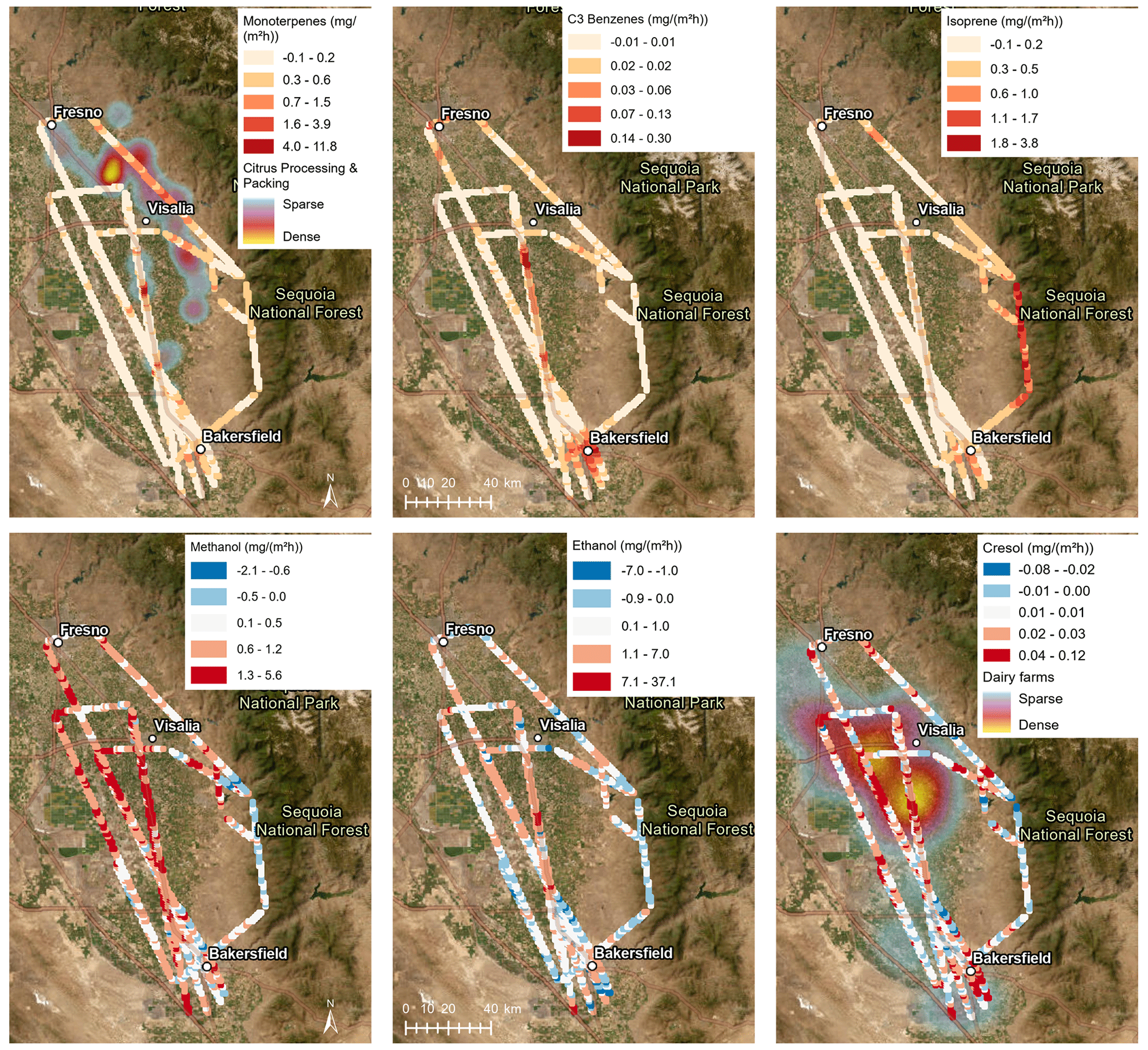
Figure 2 Fluxes in the San Joaquin Valley shown for six example VOCs. Values result from all flights, averaged to a 1 km grid (points enlarged for better visibility). Blue colors indicate deposition fluxes. The monoterpene emission distribution is shown together with a heat map of citrus packing and processing facilities. Methanol, ethanol, and cresol emission distributions are comparable to the distribution of dairy and cattle farms (shown as a heat map in the last panel). Satellite imagery map from Esri ArcGIS Pro.

The mass flux measured in the San Joaquin Valley was overwhelmingly dominated by OVOCs (including alcohols, acids, carbonyls, and other OVOCs) with 81 % of the total (Fig. 3). Alcohol emissions alone contributed almost half, mostly due to methanol (21 %) and ethanol (18 %). Acids (18 %) and carbonyls (9 %) were also relevant OVOC emissions. We attribute the dominance of OVOC emissions mainly to the abundance of dairy farms in the study area (see Fig. 1 and below), with 200 farms in the flux footprints and ca. 1400 in the whole San Joaquin Valley (Hopkins et al., 2019). In an airborne study of VOC mixing ratios in the San Joaquin Valley, OVOCs even accounted for 91 % of the total (Liu et al., 2022). This reflects the fact that a relevant fraction of the reactive VOCs is lost before it reaches the point of observation, which makes it difficult to determine primary emission contributions from concentration-based studies and underscores the value of direct flux measurements.

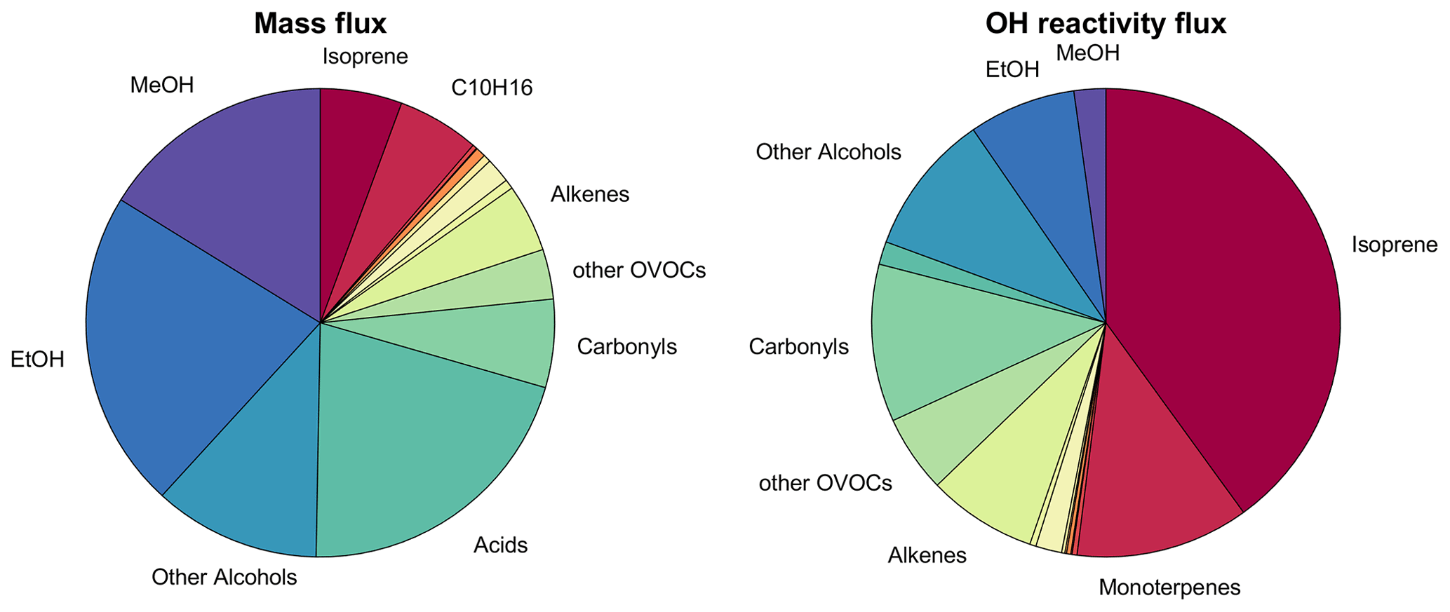
Figure 3 Pie charts showing the median composition of the measured net VOC flux mixture, with VOC group contribution to measured mass flux and OH reactivity flux. The VOCs included in each group are listed in Table S1. VOC classes contributing less than 2 % of the total were not labeled. MeOH: methanol, EtOH: ethanol.

When the fluxes are scaled by OH reactivity (Fig. 3), which is an indicator for the VOCs' relevance for ozone formation, the OVOCs contribute 42 %, but now the terpenoids (isoprene, mono- and sesquiterpenes) contribute equally 42 % of the total, mainly because of isoprene (32 %) followed by monoterpenes (10 %). This fraction is much higher than the concentration-based biogenic VOC (BVOC) contribution to OH reactivity of 6 % found in the San Joaquin Valley by Liu et al. (2022), since such observations are skewed towards long-lived species and do not reflect the primary emission contributions (see above).

When considering the relative contributions shown in Fig. 3, it is important to note that the contribution of isoprene is almost entirely due to the flight leg performed in the Sierra Nevada foothills. Depending on the wind direction, it is possible that these emissions contribute less to air quality in the center of the San Joaquin Valley than Fig. 3 suggests.

3.2 Source attribution

The San Joaquin Valley contains a multitude of potential VOC sources, with crop agriculture, dairy and cattle farms, major highways, oil and gas production, urban areas, and natural sources. In order to attribute VOC emissions to their sources, we used a footprint disaggregation method that applies multivariate linear regression of the measured fluxes using land cover information weighted by footprint density as predictors (Hutjes et al., 2010; Hannun et al., 2020). We compiled the spatial distribution of land cover types and point sources using CropScape for land cover (National Agricultural Statistics Service, 2018); Vista-CA for the locations of dairy and cattle farms, composting sites, digesters, landfills, and wastewater treatment plants (Hopkins et al., 2019); a business registry for ethanol biofuel manufacturing locations (SafeGraph, 2022); a registry of active oil and gas wells (CALGEM, 2022); and locations of citrus processing and packaging facilities collected from Google Maps which we uploaded to ArcGIS online (Pfannerstill, 2022). Using these sources as input, we first identified the crop types and Vista-CA sources that were present in at least 10 % of the footprints or covered at least 10 % of a footprint. The remaining source types were used as input for a multivariate linear regression for footprint disaggregation. The number of crop types was reduced further by performing a test that added crop types in each regression loop. Only citrus crops (combining oranges and other citrus) and other tree fruit crops (combining cherries, nectarines, peaches, pomegranates, apples, pears) significantly improved the regression. All remaining crop types were summed up under a “cropland” category. The grasslands in the slopes of the Sierra Nevada were removed from the results since they are strongly impacted by the hillslope effect, which causes pollution from the valley to be transported up along the slopes and makes it appear as positive emission fluxes in the measurements, although it is not emitted by the grass itself. Grasslands are expected to be negligible VOC sources (Bamberger et al., 2010; Brunner et al., 2007) except immediately after cutting (Brilli et al., 2012; Davison et al., 2008). Figure 4 shows the relative composition of emissions attributed to eight relevant source types found in the San Joaquin Valley.

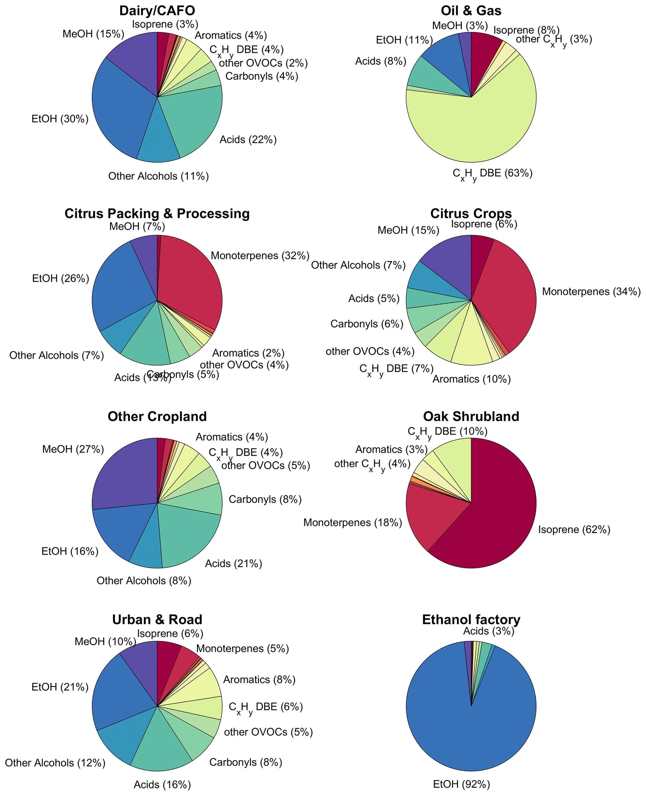
Figure 4 Pie charts showing the composition of the measured VOC emissions by mass from the footprint disaggregation result. C_xH_y DBE: hydrocarbons with double-bond equivalents (i.e., alkenes, cycloalkanes, and potentially unknown aromatics). For oil and gas sources, this category includes C₁₅H₂₄ (European Chemical Agency, 2006) and C₁₀H₁₆ (Gueneron et al., 2015) isomers that are sorted into the sesquiterpene and monoterpene categories, respectively, for other sources. Since the PTR-MS is blind to most alkanes, the VOC composition, especially of the oil and gas category, can be expected to be incomplete.

The footprint disaggregation results (Fig. 4) show reasonable emission compositions for the sources presented, although the separation of sources is not always complete. For example, the oil and gas category includes isoprene, since most of the oil and gas wells overflown were located in the Sierra Nevada foothills northeast of Bakersfield, close to the oak woodlands. Vice versa, the oak shrubland category includes hydrocarbons that may stem from the oil and gas production (but partly may be PTR-MS fragment ions from terpenoids emitted in the oak region; Kari et al., 2018; Tani, 2013).

Apart from the overall composition of each source's emissions, we also identified tracer $m/z$ for the sources (Table 2). These were $m/z$ values whose emissions in the disaggregation result were above 3 × the overall median emission of that $m/z$, above 2 × the standard deviation of emissions between the sources, and higher than in the disaggregation result of at least six other source categories.

Table 2 List of tracer $m/z$ values specific to the different sources, resulting from the footprint disaggregation. Point source emissions are given in kilograms per facility per hour and area source emissions in mg m⁻² h⁻¹. The complete disaggregation results with emissions of each VOC attributed to each source are given in Table S2. No specific tracers were found for the general cropland emissions. DBE: double-bond equivalents.

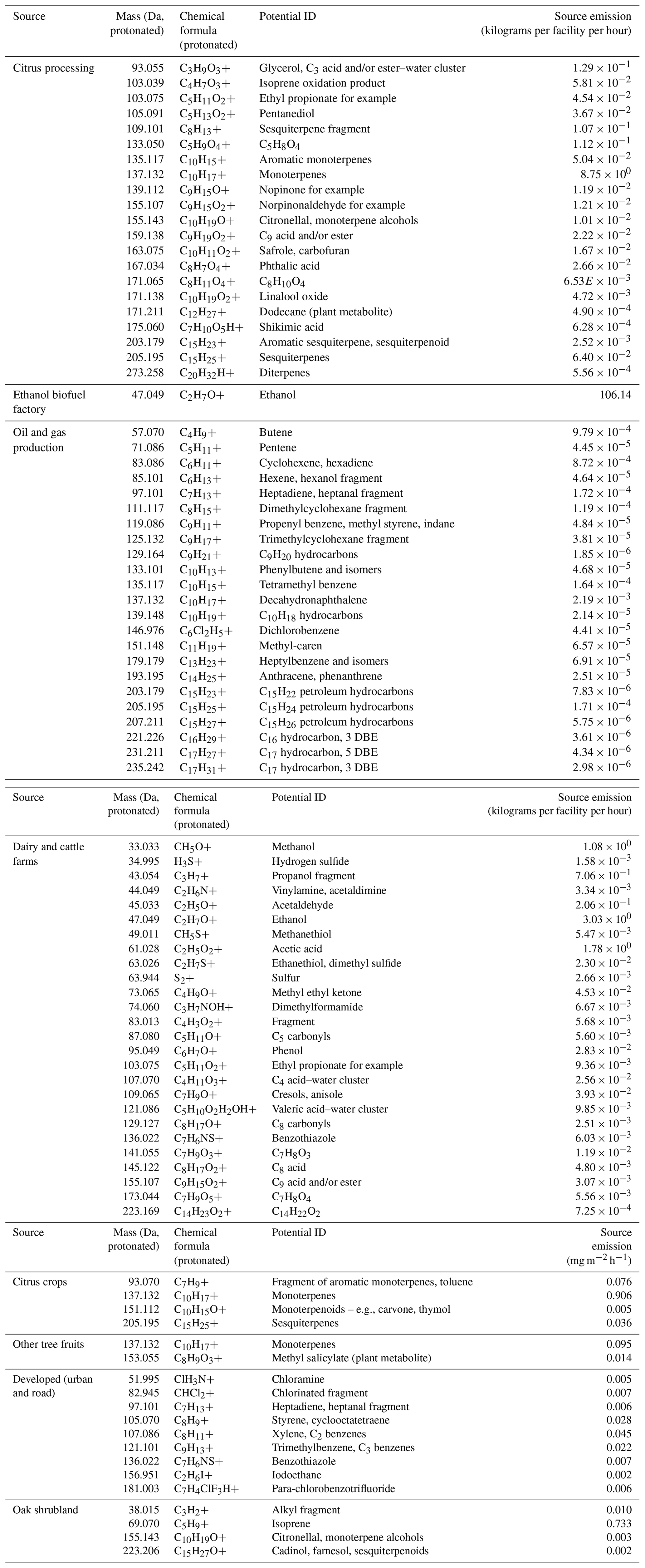
The composition of the dairy–CAFO (concentrated animal feeding operation) category was dominated by fermentation-related VOCs, with a mass fraction of 12 % methanol (1.1 kg per facility per hour), 34 % ethanol (3.0 kg per facility per hour), 12 % other alcohols, and 21 % acids dominated by acetic acid (1.8 kg per facility per hour) (Fig. 4, Table 2). This composition is in agreement with direct measurements of dairy cattle VOC emissions (Gierschner et al., 2019; Oertel et al., 2018; Shaw et al., 2007; Stackhouse et al., 2011; Sun et al., 2008; Yuan et al., 2017a); of silage, the fodder used for cows in industrial agriculture (Hafner et al., 2013; Malkina et al., 2011); and of manure (Hales et al., 2015; Sun et al., 2008), which all are rich in alcohols and acids. For example, Yuan et al. (2017a) reported a mole fraction of 55 %–87 % alcohols and 4 %–32 % carboxylic acids from CAFO emissions. Less important in terms of amount but relevant “tracers” for dairy and cattle emissions (Table 2) in agreement with previous studies (Yuan et al., 2017a; Borhan et al., 2012; Gierschner et al., 2019) also included strongly odor-active sulfur-containing VOCs (hydrogen sulfide, methanethiol, dimethyl sulfide or ethanethiol, benzothiazole) and phenolic species (phenol, cresols). The emission strengths can vary strongly between individual dairy farms (Gentner et al., 2014a; Yuan et al., 2017a) based on feed composition (Hafner et al., 2013; Hales et al., 2015; Malkina et al., 2011), management practices, or animal age and state (Shaw et al., 2007; Gierschner et al., 2019; Stackhouse et al., 2011). This is confirmed by our observations, where, e.g., methanol fluxes from dairy-dominated footprints had a variance of 2.2 mg m⁻² h⁻¹ associated with a median of 1.0 mg m⁻² h⁻¹.

The oil and gas category mainly consisted of hydrocarbons (82 %, Fig. 4). Since the PTR-MS method is blind to most alkanes, we can only report hydrocarbons with double bonds or longer-chain (cyclo)alkanes and aromatics. Interestingly, two $m/z$ values that are usually attributed to biogenic emissions were significantly enhanced in the oil and gas emissions: C₁₅H₂₄H⁺ ($m/z$ 205.19) and C₁₀H₁₆H⁺ ($m/z$ 137.13; Table 2). In the oil and gas category, we attributed them to petroleum emissions and included them in the category of hydrocarbons with double-bond equivalents, since C₁₅H₂₄ can be a component of petroleum kerosene (European Chemical Agency, 2006) and C₁₀H₁₆H⁺ here is likely a PTR-MS product of decahydronaphthalene (Gueneron et al., 2015). Tracers for this source category included C₄–C₁₇ hydrocarbons, covering almost the entire mass and volatility range that can be measured with the method used. Example $m/z$ values are (i) C₁₄H₂₄H⁺ (anthracene or phenantrene) and (ii) C₈H${}_{\mathrm{15}}^{+}$ and C₉H${}_{\mathrm{17}}^{+}$, which both are fragments of substituted cyclohexanes (Gueneron et al., 2015).

The citrus packing and processing category includes juice factories, fragrance extraction, and citrus packaging facilities. Emissions from these consist of 28 % (8.75 kg per facility per hour) monoterpene and 28 % ethanol emissions as the largest contributors by mass (Fig. 4). While there were 45 citrus processing and packaging facilities identified in the study area, one of them stood out with extremely large emissions: a facility in Tipton, CA. In Fig. 2, this shows up as the largest-monoterpene-source location, with 11.8 mg m⁻² h⁻¹ emitted on average in Tipton over all flights, while only a small fraction of the measurement footprint is covered by the facility. This facility not only produces juices but also extracts monoterpenes for the fragrance industry (Ventura Coastal, 2023). It is possible that ethanol is used as a solvent in the extraction process. Also, fruit juices contain significant amounts of ethanol (Gorgus et al., 2016). Since citrus fruits emit monoterpenes, especially when they are being handled, and monoterpene emissions were enhanced around citrus packaging facilities, we conclude that citrus packing also contributes to the agroindustrial source of monoterpenes summed up in this category. Tracers observed in the citrus processing and packing emissions (Table 2) were rich in C₁₀H₁₆ monoterpenes but also included aromatic monoterpenes (C₁₀H₁₅), monoterpenoids (e.g., C₁₀H₁₈O, C₉H₁₄O, C₉H₁₄O₂, C₁₀H₁₈O₂), sesquiterpenes (C₁₅H₂₄), sesquiterpenoids (C₁₅H₂₂), diterpenes (C₂₀H₃₂), and the plant metabolite dodecane (C₁₂H₂₆).

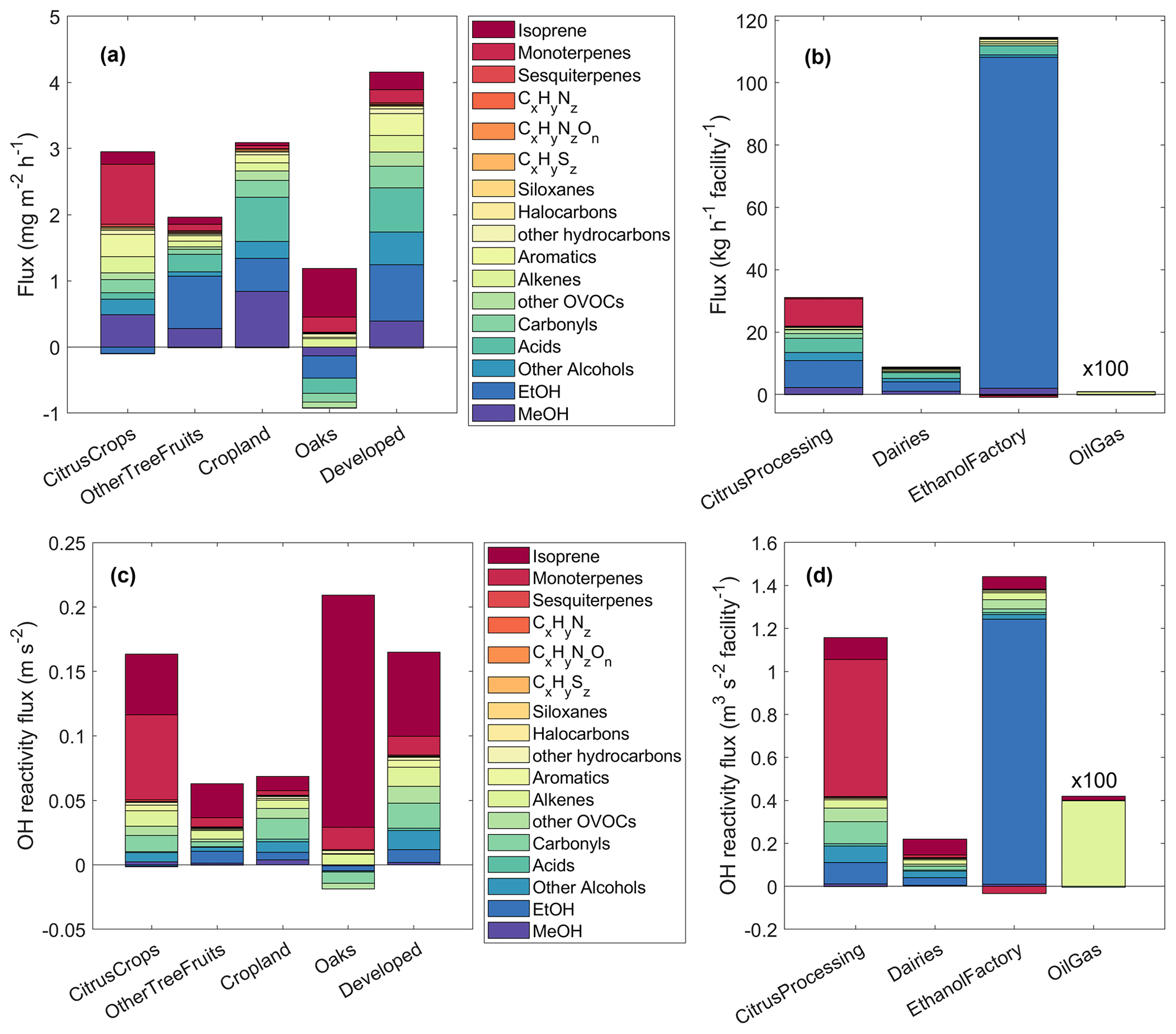
Figure 5 Quantitative footprint disaggregation results shown as mass fluxes (a, b) and OH reactivity fluxes (c, d). The fluxes for area sources were given per area (a, c), while point sources (b, d) are reported as fluxes per facility. Negative fluxes signify deposition. Note that the oil and gas well emissions were multiplied by 100 to become visible and that their expectedly significant alkane emissions were not captured by the measurements. “Developed” includes urban areas and roads. MeOH: methanol, EtOH: ethanol.

The citrus crop emission composition with mass fractions of 31 % monoterpenes and 17 % methanol agrees with a study performed on Californian citrus plants and in a San Joaquin Valley citrus plantation, where methanol and monoterpenes were the largest emissions, approximately equal in molar contributions (Fares et al., 2011, 2012). The aromatic fraction of the citrus crop emissions (11 %) included aromatic monoterpenes (C₁₀H₁₅) and their fragments. Other aromatic emissions from citrus observed here (toluene, Table 2) have previously been reported as well (Misztal et al., 2015).

Emissions of the “other tree fruits” category (not shown in Fig. 4 for space reasons; see Fig. 5 and Table 2) were enhanced in monoterpene emissions compared to the other cropland, and they exhibited a plant metabolite as a tracer: methyl salicylate, a methyl ester of a plant hormone that is considered to be a stress indicator (Niinemets and Monson, 2013). The monoterpene enhancement is in accordance with the literature, where fruit trees such as cherry and peach have been shown to be monoterpene emitters (e.g., Gentner et al., 2014b; Rapparini et al., 2001).

The emission mass fractions in the “other cropland” category look similar to the dairy emissions, which is likely because the dairy farms are usually located in the middle of cropland and cannot completely be separated out. However, in the cropland category, the methanol emission fraction is, at 27 % of the total, much higher than in the dairy category (Fig. 4), which indicates that some actual crop emissions were captured by the disaggregation. Methanol has been reported to be emitted by many crops (König et al., 1995; Das et al., 2003; Gonzaga Gomez et al., 2019; Karl et al., 2001; Warneke, 2002; Gentner et al., 2014b; Loubet et al., 2022), including almonds (Gentner et al., 2014b), one of the major crops in the San Joaquin Valley. There were no specific tracer VOCs identified for the “other cropland” category.

The oak shrublands emissions were dominated by isoprene (62 %, 0.73 mg m⁻² h⁻¹) and monoterpenes (20 %, Fig. 4). The oaks of the Sierra Nevada foothills are known isoprene emitters (Misztal et al., 2014). Tracer $m/z$ values identified for the oak shrubland emissions also included monoterpene alcohols (C₁₀H₁₈O) and sesquiterpene alcohols (C₁₅H₂₆O).

The emission composition of the urban and road category was similar to the composition of VOC emissions in Los Angeles (Pfannerstill et al., 2023a), with a large ethanol contribution (21 %, Fig. 4) and significant aromatics emissions (8 %). Tracer species identified for this source category included chloramine (potentially from cleaning; Mattila et al., 2020); several aromatics (styrene; C₂ benzenes, e.g., xylene; C₃ benzenes, e.g., trimethylbenzene) indicative of traffic emissions; and para-chlorobenzotrifluoride, a coating solvent (Stockwell et al., 2021).

In Pixley, CA, the largest single ethanol source of the study area was observed: an ethanol biofuel factory, which according to the disaggregation emits 106 kg of ethanol per hour. The footprint disaggregation result of almost exclusively ethanol emissions (93 %, Fig. 4) for this facility is reasonable.

Figure 5 shows quantitative results of the footprint disaggregation. Area fluxes per mass (Fig. 5a) were highest in the “developed” category (total of ∼4.2 mg m⁻² h⁻¹), which includes roads and urban areas, followed by cropland and citrus crop emissions of ∼3 mg m⁻² h⁻¹ each. A notable result was the deposition of OVOCs (alcohols, acids, carbonyls) of −0.9 mg m⁻² h⁻¹ in total in the oak shrublands. With an emission flux of 1.1 mg m⁻² h⁻¹, the resulting net mass flux of the oak shrublands was close to zero. Deposition of oxygenated VOCs on leaf surfaces and even uptake into leaves (Seco et al., 2007; Canaval et al., 2020) and soils (Rinnan and Albers, 2020) are known phenomena. Point source emissions (Fig. 5b) were highest from ethanol biofuel manufacturing (∼115 kg per hour per facility), followed by citrus processing and packing (∼31 kg per hour per facility), and dairy farms (∼9 kg per hour per facility).

Considering the OH reactivity instead of the mass of emissions by area (Fig. 5c) changes the order of source importance: the oaks were the largest source of OH reactivity per area (0.21 m s⁻²) followed by citrus crops (0.17 m s⁻²) and developed areas (0.16 m s⁻²). Among the point sources, scaled by OH reactivity, the ethanol manufacturing factory (Fig. 5d) was still largest (0.59 m³ per second squared per facility) and was closely followed by citrus processing (0.43 m³ per second squared per facility). Dairy farms emitted an OH reactivity of 0.22 m³ per second squared per facility.

The relevance of each of these sources for air quality in the San Joaquin Valley depends on their abundance in the region. It should be noted that there is only one ethanol biofuel factory in the valley but ca. 1400 dairy farms, 47 000 active oil or gas wells, and 45 citrus processing facilities. The areas of citrus crops, other tree fruits, other cropland, oak shrublands, and developed areas in the whole San Joaquin Valley are approximately 970, 1140, 17 540, 3880, and 3960 km², respectively. (The oak area depends strongly on where the border of the valley is drawn.) Previous studies have reported that dairy farms are a major contributor to ozone formation in the San Joaquin Valley, second only to road transport (Howard et al., 2008), and predicted that traffic and dairies would contribute equally by 2020 (2012). We refrain from upscaling our results to the whole San Joaquin Valley for two reasons: the source separation resulting from the disaggregation is not perfect, and the contribution of the oak woodlands depends strongly on where along the slope of the Sierra Nevada the border of the valley is drawn. However, it becomes clear from our observations that citrus-related emissions – including crops and citrus processing or packing – are a previously disregarded source of highly reactive VOCs in the San Joaquin Valley with important ozone formation capabilities. Locally, in Pixley, ethanol biofuel manufacturing is a substantial VOC source with potential for secondary air pollution contribution.

3.3 Inventory comparison

A comparison of observed median fluxes with the California Air Resources Board (CARB) inventory and the combination of the BEIS (biogenic) and FIVE-VCP (anthropogenic) inventory, hereafter “BEIS + FIVE-VCP”, is given in Fig. 6. In both inventories, median isoprene emissions were strongly overestimated. In the CARB inventory (Fig. 6a), methanol, acetaldehyde, and acetone emissions were relatively close to the observations (within a factor of 2). All other CARB VOCs included were underestimated in the medians, notably the aromatics and typical dairy emissions such as ethanol, acids, cresol, and phenol.

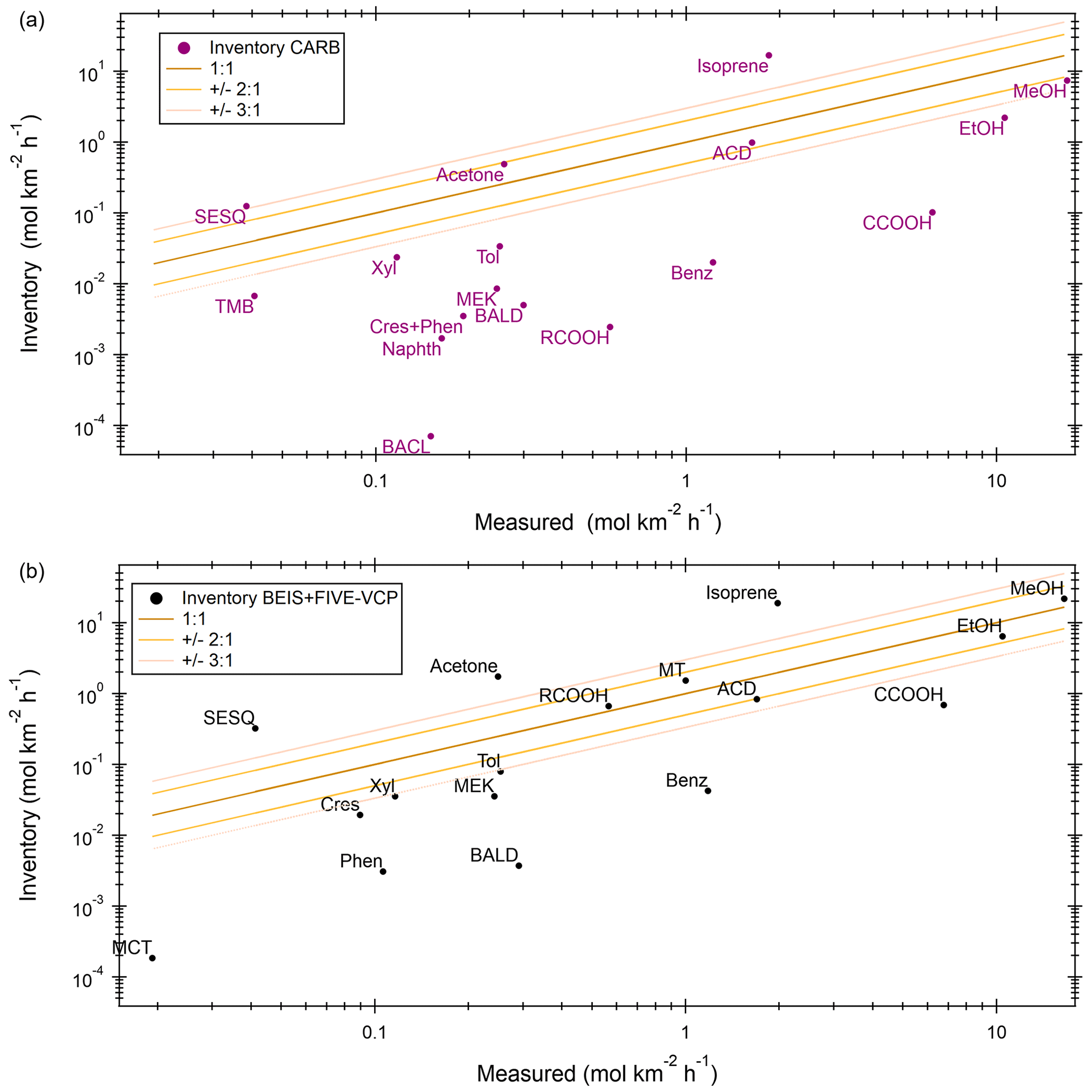
Figure 6 Comparison of median values between measured and inventory emissions of individual VOCs for (a) CARB and (b) BEIS + FIVE-VCP. Cres: cresol, Phen: phenol, MCT: methanethiol, SESQ: sesquiterpenes, TMB: trimethylbenzene, BALD: benzaldehyde, BACL: biacetyl, Naphth: naphthalene, MEK: methyl ethyl ketone, Benz: benzene, Xyl: xylene, Tol: toluene, MT: monoterpenes, MeOH: methanol, EtOH: ethanol, CCOOH: acetic acid, ACD: acetaldehyde, RCOOH: higher organic acids. “Measured” values can slightly differ in comparison to each inventory because of a different distribution and different coverage of inventory grid cells.

While most CARB inventory VOC emissions were lower than observations, the BEIS + FIVE-VCP inventory emissions (Fig. 6b) scatter more around the 1:1 line with observations. Within a factor of 2 were methanol, ethanol, monoterpenes, long-chain acids, and acetaldehyde; within a factor of 3 were toluene and xylene. The inventory underestimated the median emissions of cresol, phenol, benzaldehyde, benzene, and acetic acid and overestimated acetone and potentially sesquiterpene emissions. The sesquiterpene emissions observations are a lower limit because their speciation is unknown, and conservative reaction rates were assumed for the correction of ozone and OH loss between surface and flight altitude.

Since emissions are spatially highly variable within the San Joaquin Valley according to source distribution, spatial comparisons of observed emissions with the inventories provide additional information and can regionally differ from the median comparison shown in Fig. 6. Figure 7 shows the difference between measurements and inventory for isoprene and monoterpene emissions. Both inventories display similar patterns for isoprene (Fig. 7a and b). Observations and inventories matched well in the oak shrublands, with only a slight tendency towards overestimation, especially in the BEIS inventory, potentially because of the reduced fraction of live oak trees (see Fig. S6 and Sect. 3.1). Isoprene emissions were strongly overestimated by both inventories northeast of Visalia, in the region with intense citrus production (see Fig. 7d). The CARB inventory overestimated isoprene emissions in Bakersfield, while the BEIS + FIVE-VCP inventory matched relatively well there and instead showed a stronger overestimation in the dairy region around Hanford. For monoterpene emissions (Fig. 7c and d), the two inventories were distinctly different. The CARB inventory underestimated monoterpene emissions almost throughout the study region, with especially strong underestimations in the regions with intense citrus processing. The monoterpene emission hotspots of the juice and fragrance factory in Tipton (and to a lesser extent of a juice factory in Delano) have clearly not been included in either of the two inventories. Contrary to the CARB inventory, the BEIS + FIVE-VCP inventory overestimated monoterpene emissions from large swaths of the croplands. However, it underestimated monoterpene emissions in the citrus regions similarly to the CARB inventory. Unrealistic land cover underlying the inventory is likely the reason for mismatches between observed and predicted isoprene and monoterpene emissions (Misztal et al., 2016).

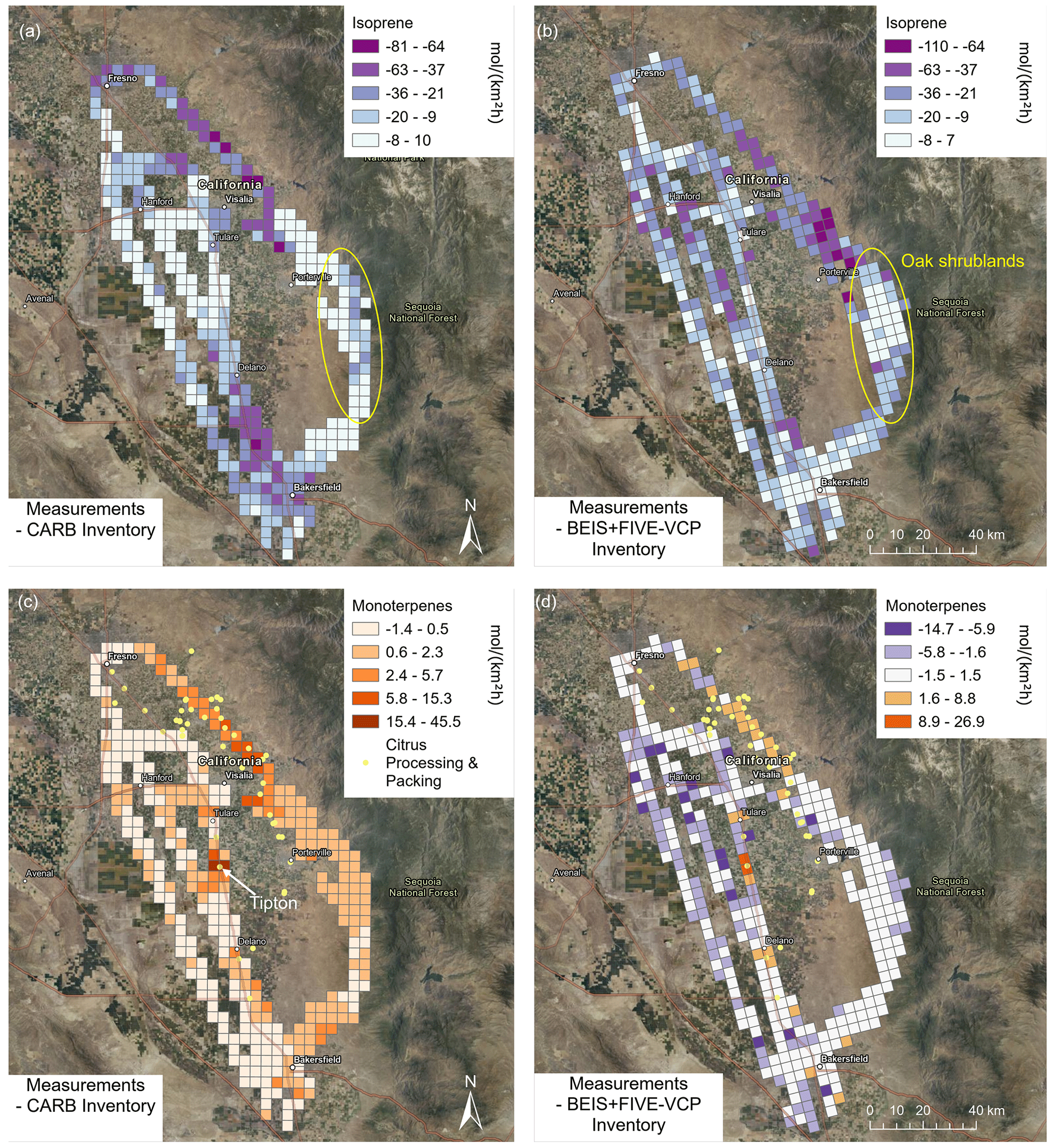
Figure 7 Differences between measurement and inventory emissions for terpenoids observed in the San Joaquin Valley. (a, c) CARB inventory. (b, d) BEIS + FIVE-VCP inventory. Orange colors designate observations > inventory emissions, purple colors the opposite. Color scales were chosen accordingly (diverging where there are both over- and underestimations in the inventory, orange where there are mainly underestimations and purple where there are mainly overestimations). Important sources are indicated in the maps (oak shrublands for isoprene, citrus processing and packing for monoterpenes, with Tipton highlighted as the place with a juice and fragrance extraction factory). Satellite maps from NAIP imagery via Esri ArcGIS Pro.

The benzenoid emissions comparison (Fig. 8) showed distinct patterns where toluene and xylene were both underestimated by the inventories along the highway and in Bakersfield but overestimated in Fresno and Visalia. Toluene emissions were also underestimated in the citrus production regions northeast of Visalia, potentially because of citrus toluene emissions (Misztal et al., 2015), but this signal may be influenced by fragments of aromatic monoterpenes (Kari et al., 2018).

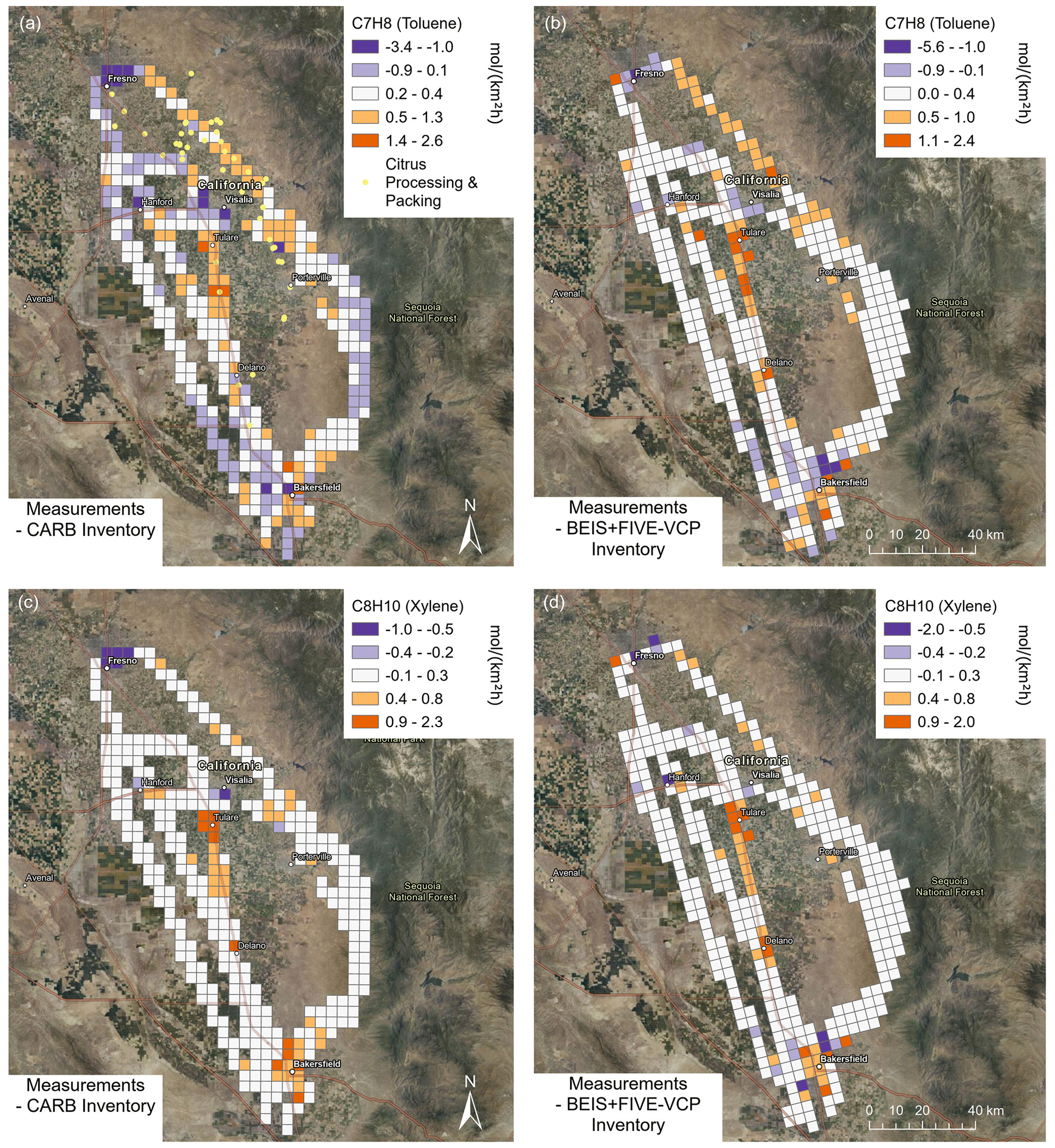
Figure 8 Differences between measurement and inventory emissions for two aromatic VOCs observed in the San Joaquin Valley. (a, c) CARB inventory. (b, d) BEIS + FIVE-VCP inventory. Satellite maps from NAIP imagery via Esri ArcGIS Pro. Orange colors indicate where the inventory is underestimating emissions and purple colors where it is overestimating them. The C₇H₈ signal potentially includes fragments of aromatic monoterpenes besides toluene.

Typical dairy VOC emissions are shown in comparison with the inventories in Fig. 9, and they all tend to be underestimated. Both inventories predicted lower-than-observed methanol emissions with especially strong differences in the dairy-intense regions (Fig. 9a and b), while matching reasonably well in the urban areas of Bakersfield and Fresno. However, the differences were generally larger in the CARB inventory than in the BEIS + FIVE-VCP inventory. For ethanol emissions (Fig. 9c and d), the ethanol biofuel factory was the location of the largest underestimation in both inventories. Both inventories also clearly underestimated ethanol emissions in the dairy-intense regions and matched better in the urban areas. Cresol and phenol were underestimated by both inventories not only in the dairy regions but also in the urban areas. For other dairy-relevant emissions not shown here (e.g., methanethiol and acetic acid), we find a similar result where the inventories underestimate these emissions. This may explain why a model based on the CARB inventory underestimates observed enhanced ozone near dairy farms (Cai et al., 2016).

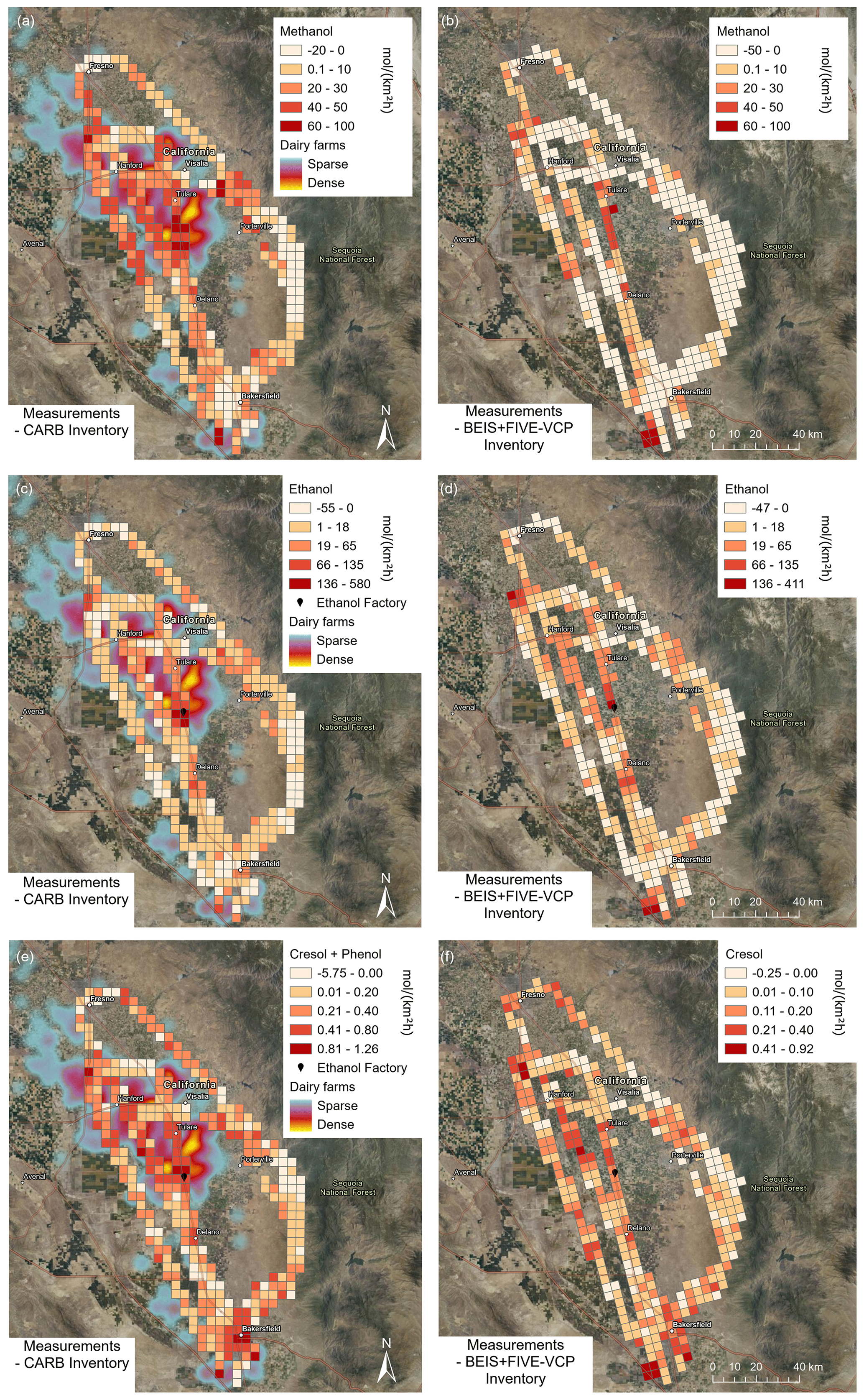
Figure 9 Differences between measurement and inventory emissions for some dairy and cattle farm VOC emissions observed in the San Joaquin Valley. (a, c, e) CARB inventory. (b, d, f) BEIS + FIVE-VCP inventory. Important sources are indicated by the density of dairy farms and, for ethanol (c, d), by the ethanol biofuel factory location. The CARB inventory includes the sum of cresol and phenol (e), while cresol is shown separately for BEIS + FIVE-VCP (f). Satellite maps from NAIP imagery via Esri ArcGIS Pro.

This hypothesis is further explored in Fig. 10, which shows ratios of OH reactivity emissions (summed from all available VOC emissions, not including deposition fluxes) between inventories and observations. Because of the strong overestimation of highly reactive isoprene emissions almost throughout the study region (see Fig. 7), the emission of OH reactive species was overestimated by a factor of at least 2 by the two inventories almost everywhere (Fig. 10a and b). However, the CARB inventory clearly shows some underestimation of OH reactive emissions (by a factor of 2–5) in the dairy-intense region, which also includes the two largest single sources of OH reactivity observed: the ethanol biofuel factory in Pixley and the citrus processing facility in Tipton, just north of Pixley (see Fig. 7). These were also the locations where the BEIS + FIVE-VCP inventory underestimated the flux of OH reactive emissions. Since overestimated isoprene in the inventories was clearly dominant in causing the OH reactivity flux mismatch, we removed it from the sums in Fig. 10c and d. Now it becomes apparent that the CARB inventory underestimated the remaining OH reactive emissions throughout the study region, usually by a factor of 3 and more. For BEIS + FIVE-VCP, the picture is different, with underestimated OH reactive emissions of a factor of 3 and more in the oak shrublands (pointing at missing biogenic VOCs) and underestimation at dairy farms at the south and northwest ends of the flight tracks and at the abovementioned citrus and ethanol processing facilities. In the urban areas, the BEIS + FIVE-VCP inventory had a tendency towards overestimating the OH reactivity source. In conclusion, our observations support the finding by Cai et al. (2016) that the dairy farm regions emit more ozone-relevant VOCs than predicted by the CARB inventory. However, some of this is not solely caused by dairy farms because intense point sources of monoterpenes and ethanol contribute to the mismatch.

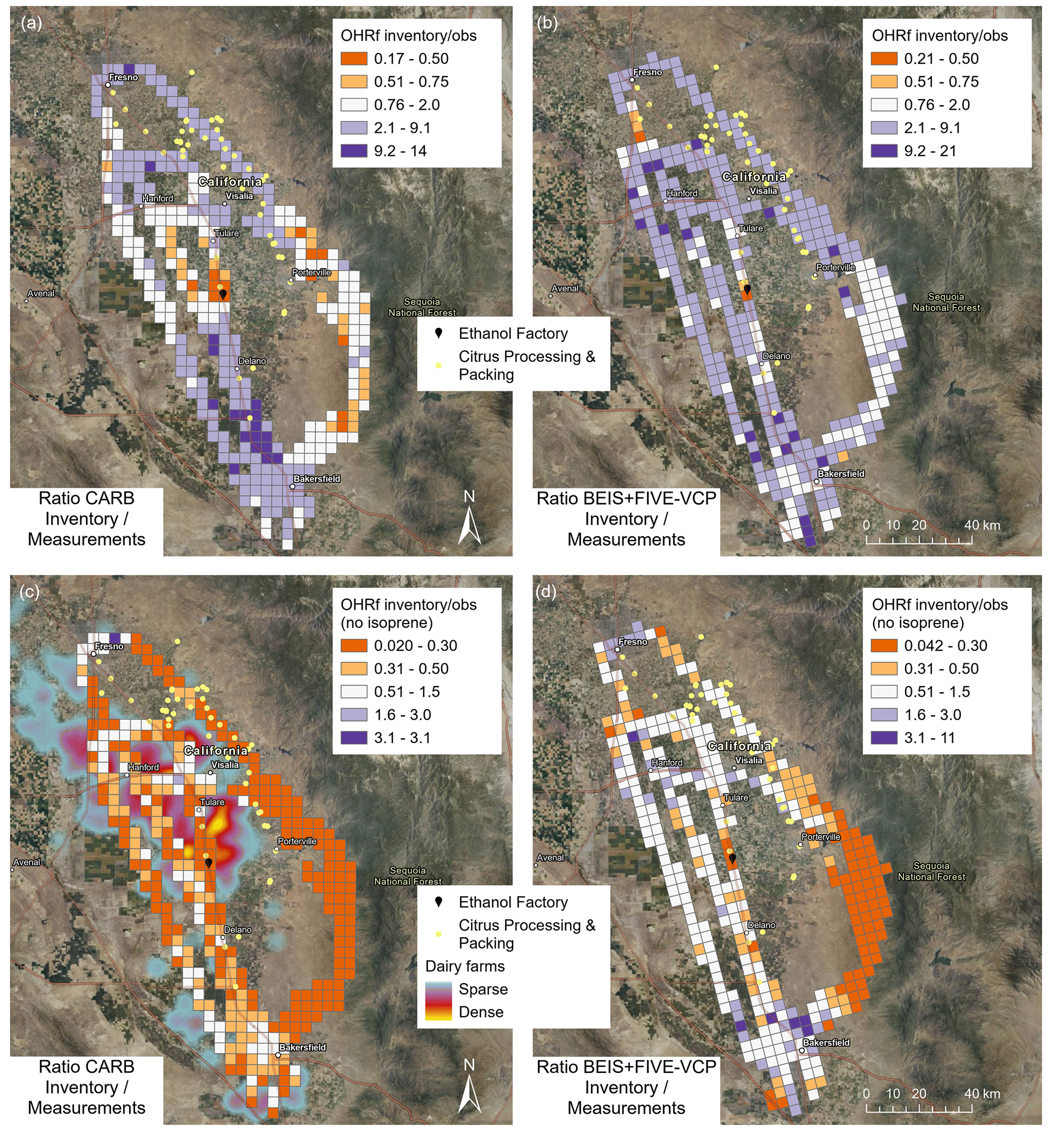
Figure 10 Inventory $/$ observations ratio of OH reactivity emissions (OHRf) summed from all VOCs for (a) CARB and (b) BEIS + FIVE-VCP; inventory $/$ observations ratio of summed OH reactivity emissions without isoprene for (c) CARB and (d) BEIS + FIVE-VCP. Satellite maps from NAIP imagery via Esri ArcGIS Pro. Orange colors indicate where the inventory is underestimating emissions and purple colors where it is overestimating them.

3.4 Temperature relationship of VOC emissions

The flight days were chosen so that measurements were conducted under a wide range of summer temperatures. Average flight temperatures ranged from 23 to 36 ^∘C (Table 1). In order to investigate measured and inventory flux dependence on temperature, the data were sorted into three different temperature bins. All data points in grid cells that were not covered in at least six out of seven flights and in each temperature bin were removed. The non-temperature-related point sources of the ethanol production and citrus extraction facilities were also removed from the temperature dependence analysis. Figure 11 shows a comparison of the observed fluxes with the two inventories grouped by those temperature bins. The inventories parameterize biogenic emissions for dependence on temperature and light (Guenther et al., 2012). Anthropogenic emissions are not explicitly parameterized for dependence on temperature. Instead, their temperature dependence is accounted for through the application of average seasonal and diurnal temporal profiles across various VOC emission sources.

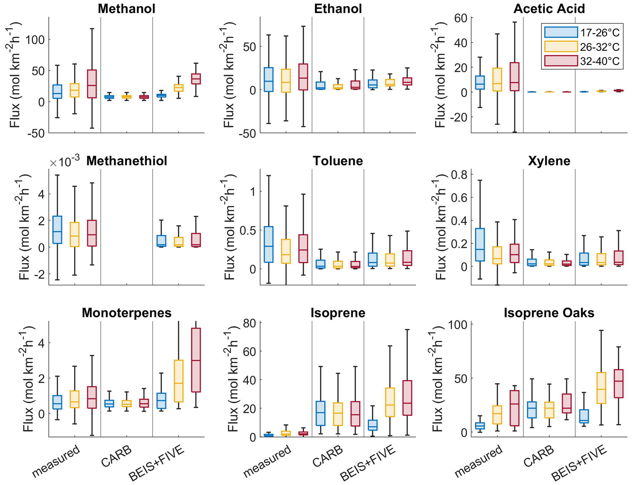
Figure 11 Fluxes of example VOCs grouped into three temperature bins, with comparison between measurements, CARB, and BEIS + FIVE-VCP inventories. All data points in grid cells that were not covered by at least six out of seven flights and in each temperature bin were removed. Each of the temperature bins includes 310–366 data points (except the subset of oak shrubland data with 20–60 data points).

Some of the observed VOC emissions increased with temperature, while others did not appear to have temperature relationships (Fig. 11). Methanol, ethanol, and acetic acid showed overall increased emissions with temperature in agreement with a study that reported increasing contributions of small oxygenated VOCs to OH reactivity in the San Joaquin Valley with increasing temperature (Pusede et al., 2015). This may be related to the main source of alcohols and acids here, dairy farms (Table 2), and specifically silage (Hafner et al., 2013), whose VOC emissions can volatilize more at higher temperatures as has been shown in experiments (Hafner et al., 2012). However, wind speed (Hafner et al., 2012) and management practices such as opening silage plastic covers (Heguy et al., 2016) play a role in this volatilization, which may explain why the temperature dependence is not more prominent in our observations. For methanol, the temperature dependence of agricultural crop emissions is a contributing factor, too (Gonzaga Gomez et al., 2019; Loubet et al., 2022). The CARB inventory did not reflect the observed emission increases in these OVOCs with temperature, while the BEIS + FIVE-VCP did better (although underestimating acetic acid emissions significantly).

Methanethiol is also a dairy farm emission, but it does not come from silage (Hafner et al., 2013). Its main source is expected to be the cows themselves (Shaw et al., 2007; Gierschner et al., 2019), and it was not temperature dependent (Fig. 11). Toluene and xylene did not display temperature-related patterns, potentially because their main source in the study region was traffic. When toluene emissions are mostly solvent related, they do increase with temperature (Pfannerstill et al., 2023b).

The biogenic VOC emissions – monoterpenes and isoprene – were clearly temperature related, as is known (Guenther et al., 2012). The observed monoterpene emission increase with temperature was not as strong as predicted by the BEIS + FIVE-VCP inventory but stronger than in the CARB inventory. The isoprene emissions were clearly temperature related in the oak woodlands, where the observed flux range was in between the CARB and BEIS + FIVE-VCP predictions. There were no significant isoprene emissions observed in the rest of the study region, especially not in the croplands (Fig. 2). Therefore, the overall isoprene emission medians were low. The overall isoprene emissions predicted by the inventories, with a clear temperature increase in BEIS + FIVE-VCP, suggest an unrealistic biogenic emission source assumed as a basis of both the inventories.

4 Conclusions

This study provides unprecedented insight into the sources and sinks of volatile organic compounds in the San Joaquin Valley, including their spatial distribution and their contribution to OH reactivity. Using a land-cover-informed footprint disaggregation method, we were able to attribute and quantify emissions of various sources and to identify tracer compounds for distinct source types.

We found that developed areas, dairies, and citrus (including citrus crops and packing or processing) are important sources of anthropogenic VOCs and reactivity in the San Joaquin Valley. Citrus processing and biofuel manufacturing sources were apparently not included in the two commonly used inventories that we compared our observations with, CARB and BEIS + FIVE-VCP. Spatially resolved differences in inventory mismatches showed that the inventories generally underestimated dairy, citrus, and highway traffic emissions but strongly overestimated isoprene emissions in the croplands. The oak woodlands in the Sierra Nevada foothills were a significant sink for oxygenated VOCs. Apart from the expected temperature dependence of biogenic VOC emissions, we also observed evidence for temperature-dependent dairy silage VOC emissions.

The results of this study provide the opportunity to improve emission inventories and have impacts for air quality modeling and policy in the San Joaquin Valley.