Modelling the impacts of emission changes on O₃ sensitivity, atmospheric oxidation capacity, and pollution transport over the Catalonia region

Tropospheric ozone (O₃) is an important surface pollutant in urban areas, and it has complex formation mechanisms that depend on the atmospheric chemistry and on meteorological factors. The severe reductions observed in anthropogenic emissions during the COVID-19 pandemic can further our understanding of the photochemical mechanisms leading to O₃ formation and provide guidance for policies aimed at reducing air pollution. In this study, we use the Weather Research and Forecasting model with Chemistry (WRF-Chem) coupled with the urban canopy building effect parameterization and building energy model (BEP + BEM) to investigate changes in the ozone chemistry over the metropolitan area of Barcelona (AMB) and its atmospheric plume moving northwards, which is responsible for the highest number of hourly O₃ exceedances in Spain. The trajectories of the air masses from the AMB to the Pyrenees are studied with the Lagrangian FLEXible PARTicle dispersion model with WRF (FLEXPART-WRF). The aim is to investigate the response of ozone chemistry to reduction in precursor emissions (NO_x – nitrogen oxides; VOCs – volatile organic compounds). The results show that, with the reduction in emissions, (1) the ozone chemistry tends to enter the NO_x-limited or transition regimes, but highly polluted urban areas are still in the VOC-limited regime; (2) the reduced O₃ production is overwhelmed by reduced nitric oxide (NO) titration, resulting in a net increase in the O₃ concentration (up to 20 %) in the evening; (3) the increase in the maximum O₃ level (up to 6 %) during the highest emission-reduction period could be attributed to an enhancement in the atmospheric oxidants hydroxyl and nitrate radical (OH and NO₃) given their strong link with O₃ loss or production chemistry; (4) the daily maximum levels of ozone and odd oxygen species (O_x) generally decreased (4 %) in May – a period with intense radiation which favours ozone production – with the reduced atmospheric OH and NO₃ oxidants, indicating an improvement in the air quality; and (5) ozone precursor concentration changes in the urban plume of Barcelona contribute significantly to the level of pollution along the 150 km south-to-north valley in the Pyrenees. Our results indicate that O₃ abatement strategies cannot rely only on NO_x emission control but must include a significant reduction in anthropogenic sources of VOCs. In addition, our results show that mitigation strategies intended to reduce O₃ should be designed according to the local meteorology, air transport, particular ozone regimes, and oxidation capacity of the atmosphere of the urban area.

1 Introduction

Tropospheric ozone (O₃) is a radiatively active gas that acts as an oxidizing agent and a surface pollutant in urban areas, where it is a major component of photochemical smog and causes a number of respiratory health effects (Sillman, 2003; Anenberg et al., 2010; Fleming et al., 2018; Sillmann et al., 2021). In 2019, it was estimated that 365 000 respiratory mortalities worldwide were due to anthropogenic O₃, representing an increase of ∼ 16 % with respect to 2010 (GBD 2019 Risk Factors Collaborators, 2020). The World Health Organization (WHO) provides guidelines to protect humans from exposure by reducing the levels of key air pollutants, including ozone. The WHO released revised air quality guidelines in 2021, keeping the O₃ levels to 100 µg m⁻³ for an 8 h daily average and recommending 60 µg m⁻³ for an 8 h daily average during the 6 consecutive months with the highest average ozone concentrations (World Health Organization, 2021).

Ozone is photochemically produced through non-linear chemical processes mainly involving reactions of nitrogen oxides (NO_x= NO₂+ NO) and volatile organic compounds (VOCs); this results from both anthropogenic and biogenic sources in the presence of sunlight (Monks et al., 2015; Crutzen, 1974; Derwent et al., 1996). This chemistry occurs in two photochemical regimes, NO_x-sensitive and VOC-sensitive (Sillman et al., 1990; Sillman, 1999). In the NO_x-sensitive regime (low NO_x and high VOCs), ozone production is controlled (or limited) by the concentration of NO_x. Therefore, the O₃ levels increase with increasing NO_x, and there are only small changes with increases in the VOC levels. In this regime, O₃ reacts mainly with hydrogenated species to form hydrogen peroxide (H₂O₂), which is removed by wet and dry deposition. In the VOC-sensitive regime (high NO_x), ozone levels increase with increased VOC concentrations and decrease with increased NO_x concentrations. This last regime is typical of urban areas, where a reduction in NO_x emissions enhances ozone levels locally due to the higher levels of oxidants (mainly hydroxyl radicals, OH) and reactions with VOCs. Peak concentrations of ozone usually occur during the midday hours, when the sunlight is most intense. However, during the afternoon and evening, high ozone concentrations are observed in remote areas due to higher biogenic VOC emissions, less titration by NO, and transport of O₃ and its precursors from their sources. At night and next to a source with high emissions of NO (e.g. power plants), ozone is lost through the process of NO_x titration and forms NO₂, which is subsequently converted to nitric acid (HNO₃) and removed from the atmosphere by wet and dry deposition (Monks et al., 2015). In summary, O₃ levels can be reduced only if there are reductions in the amounts of the precursors NO_x, VOCs, and carbon monoxide (CO). Reductions in VOC emissions would be an effective pathway to reducing ozone in a high-NO_x area (VOC-sensitive). On the other hand, reductions in NO_x emissions would be effective in reducing O₃ if NO_x-sensitive chemistry dominates. In urban areas, this photochemistry illustrates the difficulties involved in developing policies to reduce O₃ in polluted regions (Sillman, 2003). Thus, a more profound understanding of the sensitivity of local ozone formation to changes in NO_x and VOC levels is essential for developing effective air quality policies. Other important processes for removal of O₃ are reactions of halogen species (Badia et al., 2021a), which remove 30–35 Tg (11 %–15 %) of tropospheric ozone, and dry deposition, which accounts for about 20 % of the O₃ lost from the troposphere (Wild, 2007).

In addition to photochemical reactions, the concentration of ozone is sensitive to meteorological variables such as solar radiation and wind speed and direction (Neiburger, 1969). Ozone production is intensified on warm, sunny days when the air is stagnant. Therefore, the increase in the frequency, severity, and duration of heat waves during recent decades has increased the need to understand the influence of meteorological drivers and anthropogenic factors on ground-level ozone pollution. This is becoming more important for urban cities in the Mediterranean area with high summer temperatures, and heat waves are projected to become more severe in the future due to anthropogenic climate change (Pyrgou et al., 2018; Zittis et al., 2015).

Indeed, local ozone levels depend not only on local production and loss mechanisms that are sensitive to meteorological factors, but also on the transport of ozone and its precursors. Previous studies have shown that ambient ozone concentrations are strongly influenced by transport of regional ozone and its precursors, while local precursor emissions play limited roles in ozone formation (Romero-Alvarez et al., 2022; Kleanthous et al., 2014). Cristofanelli and Bonasoni (2009) showed that the background tropospheric ozone concentration in the Mediterranean area and southern Europe is affected mainly by three transport processes: (1) regional and long-range transport of pollutants, (2) downwards transport from the stratosphere, and (3) transport of dust from the Sahara.

The lockdown period provided a significant reduction in ozone precursors, and it represents an excellent opportunity to further our understanding of the photochemical reactions involved in ozone chemistry. Estimated average emission reductions in Spain during the most severe lockdown period were reported, with road and air traffic reductions reaching 80 %–90 % (Guevara et al., 2021). During this period, Guevara et al. (2021) estimated the average emission reductions at the EU-30 level to be −33 % for NO_x. Consequently, restrictive mobility measures that included important reductions in traffic had many positive environmental impacts, and improvements in air quality were reported globally (Liu et al., 2020; Venter et al., 2020; Sharma et al., 2020).

Previous modelling studies analysed the changes in air quality, emissions, and chemical regimes seen on global and regional scales during the COVID-19 lockdown (Miyazaki et al., 2021; von Schneidemesser et al., 2021; Roozitalab et al., 2022; Sicard et al., 2020; Badia et al., 2021b). A global modelling study by Miyazaki et al. (2021) showed that the global total tropospheric ozone burden declined by 6 Tg (∼ 2 %) during May–June 2020, mainly due to emission reductions in Asia and North and South America. The modelling study of Venter et al. (2020) found that, after taking into account the meteorological variations, lockdown measures reduced the levels of NO₂ (mainly due to the reduction in transportation) and the levels of particulate matter (PM) by approximately 60 % and 31 %, respectively, in 34 countries, with a general increase in O₃ of 4 % (−2 % to 10 %). Sicard et al. (2020) described ozone increases in cities (17 % in Europe, 36 % in Wuhan) resulting from lower titration of O₃ by NO due to the strong reduction in NO_x emissions from road transport. Most of this literature was focused only on the lockdown period, and the de-escalation period, which had different ozone chemistry, was not analysed. In addition, these studies did not discuss changes in the chemical regimes arising from different land uses and the transport of pollutants due to lockdown measures from cities to rural areas.

Only a few studies have reported enhanced atmospheric oxidation capacity (AOC), which describes the removal rate of primary pollutants and the formation of secondary species together with the associated O₃ increases during the COVID-19 lockdown due to increases in the major oxidants OH, hydroperoxy radical (HO₂), and nitrate radical (NO₃) (Zhu et al., 2021; Wang et al., 2021, 2022). The predominant oxidant for AOC during the daytime is OH, since NO₃ radicals photolyse rapidly during the day, which is responsible for the oxidation and removal of most natural and anthropogenic trace gases (Elshorbany et al., 2009; Saiz-Lopez et al., 2017). On the other hand, during the night, the concentration of OH is significantly reduced, and the AOC is then controlled by NO₃ together with O₃, which is also an important oxidant (Elshorbany et al., 2009; Saiz-Lopez et al., 2017). During the lockdown, the significant decreases in NO₂ concentrations increased the OH levels, which led to the formation of harmful oxidants such as O₃ (Zhu et al., 2021; Wang et al., 2021, 2022). Therefore, the AOC is an indicator used to design control policies for secondary species.

In recent decades, EU emission mitigation policies have been successful in decreasing emissions of key air pollutants such as SO₂, NO_x, non-methane VOCs – NMVOCs, and PM (Sicard et al., 2021; Agency et al., 2019). However, the current levels for the secondary air pollutant O₃ in cities continue to exceed the EU standards and the WHO air quality guidelines (Guerreiro et al., 2014; Agency et al., 2019). Indeed, local ozone pollution mitigation efforts are generally inefficient, mainly because (1) ozone formation depends on non-linear chemical interactions; (2) with a lifetime of several weeks, ozone levels are strongly influenced by long-distance transport, which is associated with specific weather conditions and the hemispheric background; and (3) its precursors are emitted mostly far from the sites of ozone exceedances. Sicard et al. (2013) found a decrease in annual O₃ averages (−0.4 % yr⁻¹) at rural sites and an increase at urban and suburban stations (0.6 % and 0.4 %, respectively) during 2000–2010 for the Mediterranean area. These changes resulted from the mitigation policies for NO_x and VOC emissions in the EU that led to an increase in O₃ levels in urban areas due to a reduction in titration by NO. Therefore, there is an urgent need to expand our knowledge of ozone chemistry to help decision-makers choose better mitigation strategies.

In the present study, we use the Weather Research and Forecasting model with Chemistry (WRF-Chem) coupled with the urban canopy building effect parameterization and building energy model (BEP + BEM) to investigate the response of NO_x–VOC–O₃ chemistry to changes in precursor emissions in the metropolitan area of Barcelona (AMB); this furthers our understanding of ozone formation mechanisms and transport to rural areas, and it enables the design of effective air quality mitigation strategies. We compare the ozone levels for two periods with very different anthropogenic and biogenic activity levels, i.e. (1) March and April 2020, when ozone precursors were at their lowest levels because of repeated lockdowns due to COVID, and (2) May 2020, when the AMB was in a relaxation plan but the ozone levels were typically highest because of the bloom of biogenic emissions under the intense sunlight conditions. In addition, ozone production regimes for different land uses of the AMB are analysed to determine changes in the $\mathrm{NO}\mathit{\text{x}}/\mathrm{VOC}$ ratio in different areas of the city that are affected by different biogeochemical effects (biogenic VOC emissions, dry deposition, anthropogenic emissions of ozone precursors). Here, we also discuss changes in the AOC oxidants and propose that the AOC should be considered when designing air quality control policies. Changes in ozone circulation from the AMB to the Pyrenees are also discussed for specific days characterized by high ozone levels.

The case study is described in Sect. 2. The air quality model, including the model set-up, validation, and simulations, is described in Sect. 3, followed by the results (Sect. 4). A discussion of the ozone chemistry that includes ozone sensitivity, AOC, and transport from the city to rural areas is presented in Sect. 5.

2 Case study

The AMB serves as our case study. It is located in Catalonia (Spain) in the north-eastern part of the Iberian Peninsula (Fig. 1). This region is characterized by a Mediterranean climate, with dry and hot summers and clear skies. Due to a complex orographic territory with different altitudes and several peripheral mountain ranges and depressions, it is not easy to generalize the climatic features of the Catalan lands for the whole territory (Martín-Vide et al., 2010). The AMB, with more than 3 million people, is the most populated urban area on the Mediterranean coast.

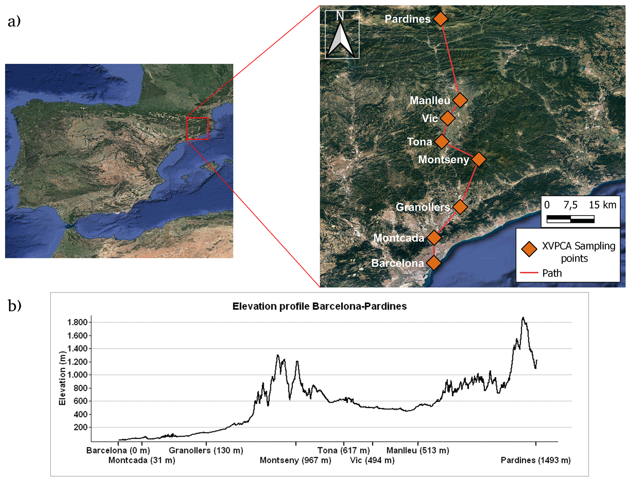
Figure 1 (a) Location and (b) main topographic features of the study area. Base maps in panel (a) were taken from © Google Earth. The locations of air pollution monitoring stations (Xarxa de Vigilància i Previsió de la Contaminació Atmosfèrica, XVPCA) along the S–N axis (Barcelona–Vic Plain–Pyrenean range) are shown in panel (a) (right).

The city of Barcelona annually reports some of the highest air pollution levels in Europe, and the most problematic pollutants are NO₂, PM_2.5, and PM₁₀ (Rivas et al., 2014). In particular, in 2019, the NO₂ annual mean levels in the high-traffic urban air pollution ground monitoring stations (Eixample and Gràcia-Sant Gervasi) exceeded the WHO guideline (40 µg m⁻³) (Rico et al., 2019). In the same year, the mean values for PM_2.5 and PM₁₀ exceeded the WHO guideline (20 and 10 µg m⁻³, respectively) at all urban stations in the city (Rico et al., 2019). Exceeding these air quality reference levels is associated with significant risks to public health (World Health Organization, 2021; Rivas et al., 2014). The year 2020 was the first year in which the NO₂ values in Barcelona remained within the WHO limits (Rico et al., 2020) due to the significant reduction in traffic emissions that resulted from the Spanish government's emergency rule and its lockdown restrictions (see Fig. S1 in the Supplement). Note that 2020 had more rainfall than previous years, which has important implications for the removal of pollutants from the air.

Another air quality problem was found for the Vic Plain (see Fig. 1), which records the highest number of exceedances for hourly O₃ levels (180 µg m⁻³) when the sea breeze transports the ozone precursors from the AMB inland to this rural plain (Querol et al., 2017; Massagué et al., 2019; Jaén et al., 2021). During the late spring and summer seasons, the combination of daily upslope winds and sea breezes may cause the intrusion of polluted air masses up to 160 km inland. Thus, the air masses from a polluted area (such as the AMB) can be transported northwards and injected at high altitudes (2000–3000 m a.s.l.) by the Pyrenean mountain range (Querol et al., 2017; Massagué et al., 2019).

Ozone levels were higher compared to previous years in Ciutadella, the background station in Barcelona, during the period March–June 2020 (see Fig. S2). In Tona (a rural station located in the Vic Plain, situated 45–70 km north of Barcelona, and surrounded by high mountains) and in Pardines (also a rural site situated in the Pyrenees; see Fig. 1), high ozone concentrations were registered and clearly exceeded the WHO limit of 60 µg m⁻³ for peak seasons. Ozone levels were high in these two rural stations during March–June, with higher values for 2015–2019 compared to 2020 due to the reduced emissions in the AMB. Note that, for some weeks, the O₃ levels were higher in 2020 than in 2015–2019 due to meteorological conditions that increased the levels of ozone precursors (see Figs. S1 and S2).

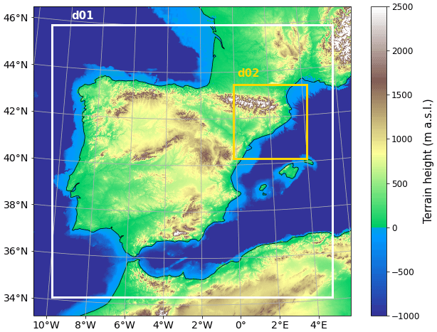
Figure 2 Model domains. D1: Iberian Peninsula 9 km × 9 km; D2: Catalonia horizontal resolution 3 km × 3 km.

In this study, we selected two periods to discuss the changes in O₃ chemistry: (1) a full lockdown period (30 March–12 April, weeks 3–4 in Table 1), in which we found the highest mobility reduction; and (2) a relaxation period (18–30 May, weeks 10–11 in Table 1), when restrictions started to relax and O₃ formation increased due to the warm temperatures of the late spring (see Table 1). The first period (30 March–12 April) was characterized by meteorological dynamism in the Iberian Peninsula. The period began with a high-pressure centre in the North Atlantic Ocean that generated a cold and dry continental north-eastern flux over Europe. General precipitation was registered in Catalonia during the first days (30 March–4 April), caused by a low-pressure centre that moved from the Atlantic to the Mediterranean. These conditions were optimal for generating precipitation in the Mediterranean area of the peninsula. The next days were defined by high pressures over Europe, which generated a more stable meteorology with isolated precipitation and a warm air mass crossing Europe from the south. During this period, no important fluxes from any directions were detected. At the surface level, the Azores anticyclone became stronger and reached pressures above 1030 hPa over the Atlantic. The second period (18–30 May) had more stability due to a strong anti-cyclonic ridge covering the south-west and centre of Europe, resulting in typical summer weather. Winds from the north and north-west were detected north-east of Catalonia and in the Ebro Valley, respectively, due to the Pyrenees' natural barrier, which modifies the trajectories of superficial winds. Low pressures were found over Italy, which intensified the winds from the north over the east of the peninsula. The last days of this period (24–30 May) registered weak precipitation in the Pyrenees and the area north-east of Catalonia, with weak winds from different directions (turning from north to south). This was caused by a strong anticyclone located in northern Europe (over 1030 hPa) that generated an undetermined situation with no effects of high or low pressures in the peninsula. See Table 1 for a summary of the meteorological conditions for these periods.

In addition, we select two days in the lockdown period (3 and 6 April) and two days in the relaxation period (22 and 26 May) on which high ozone concentrations were registered (see Table S1 in the Supplement), and there is a clear influence of the air masses from the AMB on rural areas far from the city (discussed in Sect. 5.3) for studying the changes in the O₃ circulation from Barcelona (Ciutadella) to the Pyrenees (Pardines), including the Vic Plain (Tona) and Montseny. The mean surface temperatures, pressures at the surface level, and accumulated precipitation among other meteorological variables for these days are presented for the four sites (Ciutadella, Montseny, Tona, and Pardines) in Table S2. According to the meteorological data from the Servei Meteorològic de Catalunya (2020), there was no precipitation for the days selected except in the Pyrenees (2.9 mm) on 22 May, the wind intensity was low, and the surface temperatures were significantly high for this time of the year during the two days in May.

Table 1 Meteorological conditions prevailing during the COVID-19 mobility restrictions (2020). The meteorological data were extracted from the following source: Servei Meteorològic de Catalunya (SMC). The circulation weather types (CWTs) were calculated by using the surface pressures of the NCEP and NCAR reanalysis dataset. CWTs: cyclonic 56 (C), anti-cyclonic (A), pure advectives (N, S, E, W, NE, SE, NW, SW), hybrid cyclone advectives (CN, CNE, CE, CSE, CS, CSW, CW, CNW), and hybrid anticyclone advectives (AN, ANE, AE, ASE, AS, ASW, AW, ANW). The mobility reduction over the AMB is provided in the fourth column (source: Google mobility reports (https://www.google.com/covid19/mobility/, last access: 1 February 2023)). F0, F1, F2, and F3 are the different phases of the de-escalation period, F0 being the first phase after lockdown and F3 being the last phase before all restrictions were eliminated. Psfc denotes surface pressure.

3 Air quality model

We used the regional chemistry transport model WRF-Chem (Grell et al., 2005) version 4.1, a highly flexible community model for atmospheric research in which aerosol–radiation–cloud feedback processes are considered. The WRF-Chem model is widely used for simulations of air pollution episodes (Georgiou et al., 2018; Yegorova et al., 2011) and, in particular, the air quality over the AMB has been analysed in Badia et al. (2021b).

3.1 Model set-up

The WRF-Chem model is configured with two domains covering the Iberian Peninsula (D1: 9 km × 9 km) and the Catalonia region (D2: 3 km × 3 km) with 45 vertical layers up to 100 hPa (Fig. 2). The meteorological and chemical initial and lateral boundary conditions (IC and BCs) were determined using the ERA5 global model data (Hersbach et al., 2020) and the Whole Atmosphere Community Climate Model (WACCM) (Gettelman et al., 2019), respectively. The HERMESv3 pre-processor tool (Guevara et al., 2019) was used to create the anthropogenic emission files from the CAMS-REG-APv3.1 database (Granier et al., 2019). This emission inventory is based on data from 2016. Biogenic emissions are computed online from the Model of Emissions of Gases and Aerosols from Nature v2 (MEGAN; Guenther et al., 2012). For the gas-phase chemical scheme, we used the Regional Acid Deposition Model (RADM2, Stockwell et al., 1990), which accounts for 63 chemical species, 21 photolytic reactions, and 136 gas-phase reactions. NMVOC oxidation in RADM2 only explicitly treats ethane, ethene, and isoprene species, and all other NMVOCs are classified as grouped species based on OH reactivity and molecular weight. Thus, the RADM2 gas-phase chemical mechanism grouped the VOCs into 14 species, such as alkane, alkene, aromatic, and formaldehyde. In WRF-Chem, RADM2 is coupled to the Modal Aerosol Dynamics Model for Europe (MADE)/Secondary Organic Aerosol Model (SORGAM) (Ackermann et al., 1998; Schell et al., 2001). RADM2 has been broadly used in studies of air quality over Europe (Im et al., 2015; Tuccella et al., 2011; Badia et al., 2021b), and its model biases for NO₂ and O₃ are in line with other air quality modelling studies over Europe (Im et al., 2015; Mar et al., 2016). In particular, the RADM2 chemical mechanism has been used in Badia et al. (2021b) over the AMB.

Here, we used a multi-layer urban canopy scheme, BEP + BEM (Salamanca et al., 2011)), to represent the urban areas in our domain; this takes into account the energy consumed by buildings and the anthropogenic heat, which has previously been validated for the area under study (Ribeiro et al., 2021; Segura et al., 2021). The local climate zone (LCZ) classification (Stewart and Oke, 2012) is used for the AMB, which associates specific values of the thermal, radiative, and geometric parameters of the buildings and ground with 11 urban classes, which are used by the BEP + BEM urban canopy scheme to compute the heat and momentum fluxes in the urban areas (see Segura et al., 2021, for more details on the use of the LCZ and urban morphology). We performed a spin-up of 1 month. Table 2 describes the main configuration of the model.

(Stockwell et al., 1990)(Ackermann et al., 1998; Schell et al., 2001)(Wild et al., 2000)Wesely (2007)Grell and Dévényi (2002)(Granier et al., 2019)(Guenther et al., 2012)(Salamanca et al., 2011)(Bougeault and Lacarrere, 1989)(Gettelman et al., 2019)(Hersbach et al., 2020)

Table 2 Model details and experiment configuration.

3.2 Description of the simulation cases

To better understand the impacts of emission reduction measures on air quality, the WRF-Chem model was utilized to calculate the changes in O₃ chemistry during the COVID lockdown period. We ran two simulations: (1) Business As Usual (BAU) and (2) COVID for the period of March–June 2020 (see Table 1). The COVID run used the emission changes (see Fig. 3) provided by the Barcelona Supercomputing Center (Guevara et al., 2021), which were previously used in other studies (von Schneidemesser et al., 2021; Brancher, 2021). These emission changes varied per day, country, and sector. Figure 3 displays the emission changes used in this study, and the highest changes were found for the road transport (up to 80 %) and aviation (up to 90 %) sectors. Inputs for the other emissions (biogenic, dust, sea spray) and meteorology used in WRF-Chem were set to be consistent. As a result, the differences in pollutant concentrations calculated by WRF-Chem were attributed to changes in the anthropogenic emissions.

3.3 Model validation

Several meteorological and air quality stations were used herein to evaluate the model (COVID simulation) for the lockdown (30 March to 12 April 2020) and relaxation (18 to 30 May 2020) periods. The same model configuration has been evaluated previously over the AMB for the meteorology (Ribeiro et al., 2021; Segura et al., 2021) and the chemistry, without any reduction in anthropogenic emissions (Badia et al., 2021b), for different periods.

3.3.1 Meteorology

The meteorological data used to validate our model were from the Xarxa d'Estacions Meteorològiques Automàtiques (XEMA). Stations within this network are classified as urban and rural according to the land use of the model. Herein, we used data for the wind speed (WS), temperature (T), and relative humidity (RH). Tables S3 and S4 in the Supplement present statistical evaluations of hourly data for the AMB and the Catalonia (CAT) region for the lockdown (30 March to 12 April) and relaxation (18 to 30 May) periods, respectively.

The validations of the WRF-Chem simulation (COVID run) revealed that the model generally reproduced the air temperatures of the two simulation periods well, but the performance was poorer in representing the relative humidity and the wind speed. For the first period, the simulated air temperatures for the urban stations showed low positive biases of 0.4 and 0.3 ^∘C for the AMB and CAT, respectively, and an RMSE of 1.4 ^∘C. The rural stations presented a higher bias inside the AMB (0.9 ^∘C), which resulted from erroneous descriptions of the land use at the model resolution level (3 km). Loose performance was found for the relative humidity and the wind speed, with average RMSEs of 12.2 % and 2.5 m s⁻¹, respectively. The model underestimated the relative humidity in the urban and rural areas of the AMB by 2.0 % and 5.2 %, respectively, while it overestimated the humidity in the rural areas of the CAT (1.4 %). In the case of the wind speed, the model overestimated the wind flow over the entire domain (1.5 m s⁻¹ on average in CAT), especially in the rural areas of CAT (1.9 m s⁻¹). For the second study period, a similar performance was obtained for the air temperatures inside the AMB, with a slight increase in the RMSEs (1.5 and 1.6 ^∘C for the urban and rural areas) and a decrease in the correlations between modelled and observed data (0.90 and 0.92, respectively). Unlike the first period, the model overestimated the relative humidities at all the stations in the second period, except for the rural stations in the AMB (−3.8 %). The model provided lower overestimates for the wind speeds during the second period (1.0 m s⁻¹ on average in CAT), although the correlations decreased in the second period.

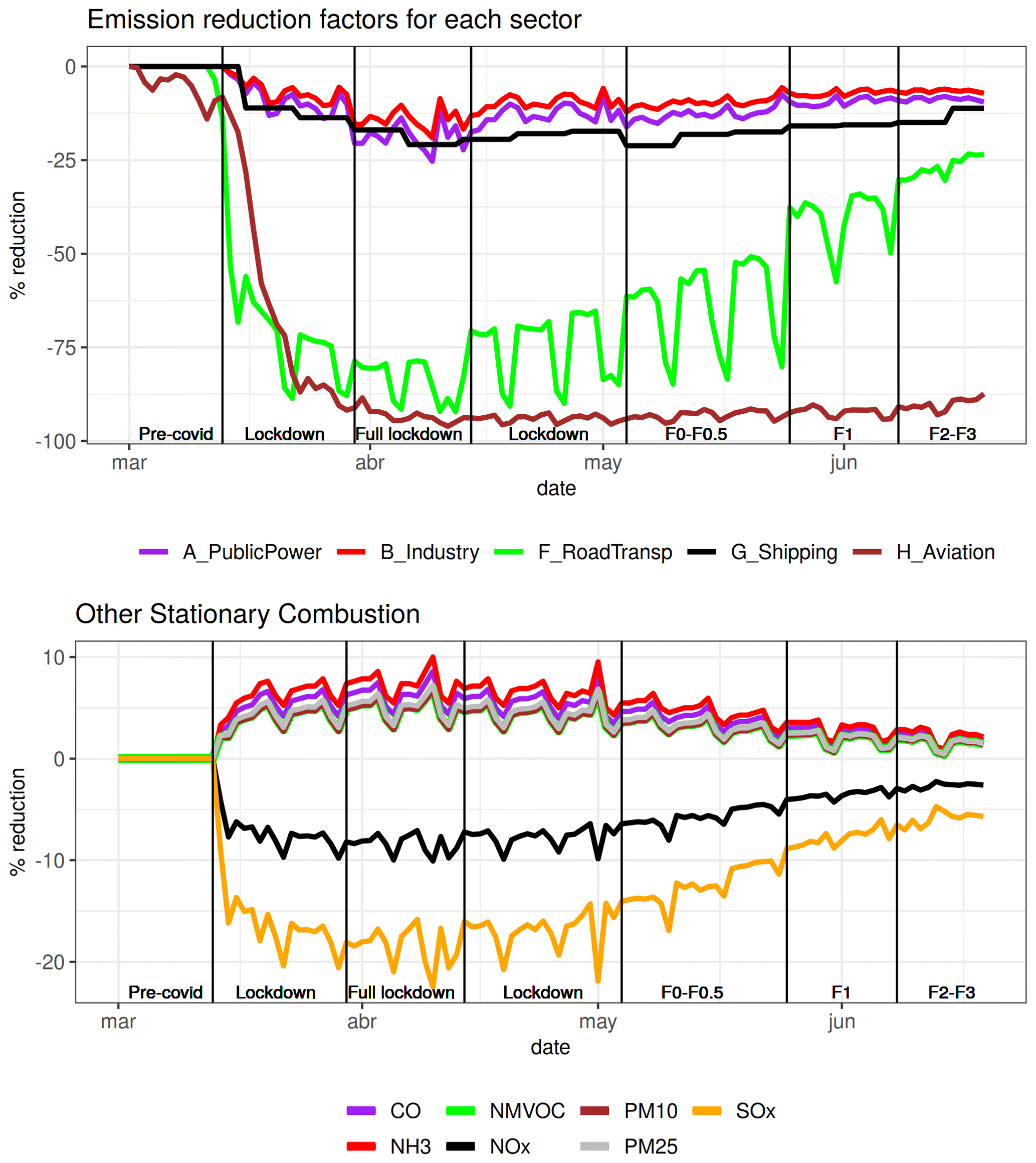
Figure 3 Emission reduction percentage (%) for each sector. Note that the other stationary combustion sector has a different reduction level for each pollutant. The periods analysed here are written at the bottom of the figure.

3.3.2 Air quality

Air quality data from the Xarxa de Vigilància i Previsió de la Contaminació Atmosfèrica (XVPCA) monitoring stations were used here. Stations in this network were classified into different groups: urban background, urban traffic, suburban background, and rural. Here, we used the data for O₃ and NO₂. Tables S5 and S6 in the Supplement present statistical evaluations of hourly data for the AMB and CAT during the lockdown (30 March to 12 April) and relaxation (18 to 30 May) periods, respectively. The modelled concentrations were converted to unit micrograms per cubic metre by using the temperatures and pressures from the model.

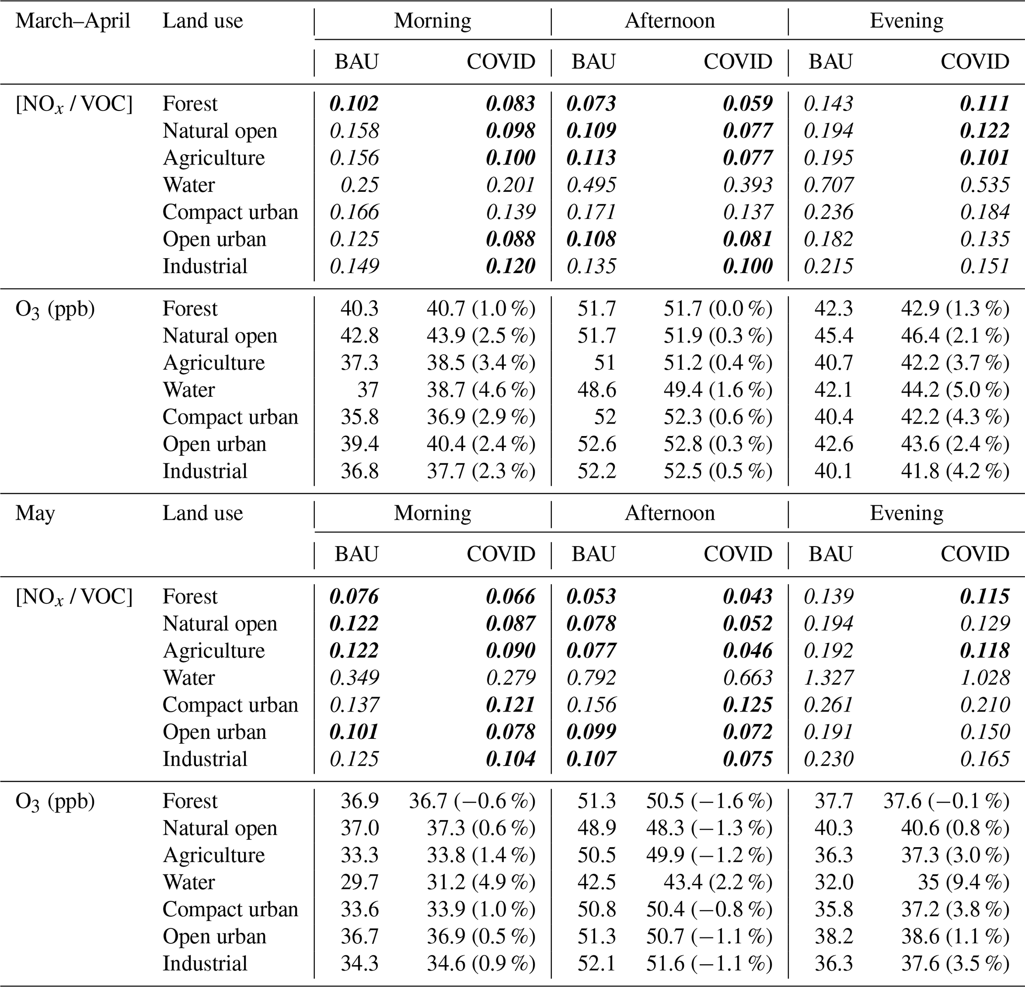
Table 3 Average NO${}_{\mathit{\text{x}}}/$ VOC ratio and ozone concentrations from 30 March to 12 April (only weekdays) and from 18 to 30 May (only weekdays) in the morning (06:00–08:00 UTC), afternoon (13:00–15:00 UTC), and evening (19:00–21:00 UTC). Italic and bold italic font indicate VOC and NO_x regimes, respectively. The relative changes in ozone concentrations (%) are shown in parentheses and were calculated as ((COVID − BAU) / BAU)×100.

Overall, the model (COVID simulation) showed reasonable agreement with the observations for NO₂ and O₃ concentrations during both periods. The best performance in the lockdown period was observed over the urban background (R between 0.43 and 0.45 for NO₂ and between 0.70 and 0.73 for O₃), while low R values were found over the rural areas (0.32 for NO₂ and 0.42 for O₃). The performance for the relaxation period was not as good as that for the lockdown period, with R values between 0.24 and 0.40 for NO₂ and between 0.42 and 0.62 for O₃. However, there were negative and positive biases in both periods for NO₂ (normalized mean bias, NMB, between −0.15 and −0.66) and O₃ (NMB between 0.13 and 0.28), respectively. Similar biases were seen in another study (von Schneidemesser et al., 2021). Part of our model bias was attributed to the (1) boundary conditions used for this study (WACCM model) that added a bias to the O₃ background levels (Giordano et al., 2015) and (2) the current emission inventory being too coarse to accurately represent the spatial distributions and temporal variations in NO_x emissions, e.g. from road transport. Low values for the modelled NO_x levels underestimated ozone loss via NO titration, which resulted in high nighttime surface ozone concentrations. The lifetime of surface NO_x (a few hours) is shorter than that of O₃ (days or weeks); thus, the surface NO_x concentrations are very sensitive to emissions. We should also mention that there might be large uncertainties for the calculations of emission factors, as discussed in Doumbia et al. (2021). Underestimates of traffic NO_x emissions over Europe have been mentioned previously in several air quality modelling studies (von Schneidemesser et al., 2021; Karl et al., 2017). Although the model exhibits biases for NO₂ and O₃, the modelled air quality changes presented in the next section are in line with other studies such as Querol et al. (2021) that present a comparison between data from years 2015–2019 and the lockdown and relaxation periods for the year 2020 in the city of Barcelona.

4 Results

4.1 Air quality changes

During the first period (30 March to 12 April) we see a general reduction in NO₂ concentrations of the COVID simulation with respect to the BAU all over the Catalonia region at the surface level, with high reductions found during the evening peaks (19:00–21:00 UTC) and over the AMB (−2 to −18 µg m⁻³, −10 % to −70 %) (see Fig. S3). The highest reductions were found around the airport due to a reduction in air traffic emissions (see Fig. 3). The surface concentrations of VOCs were slightly lower during the morning peak, with reductions up to −2 µg m⁻³ (−10 %), as can be seen in Fig. S4. Similarly, there was also a reduction during the evening peak of up to −1.5 µg m⁻³ (−12 %). Note that, during the lockdown, the VOC emissions increased up to 8 % in the stationary combustion sector (see Fig. 3). Changes in emissions that showed a significant decrease in NO₂ concentrations and a slight decrease in VOC concentrations enhanced O₃ levels over the AMB. This is consistent with the observations, where there was a decrease in NO₂ concentrations (40 %–80 %) and an increase in O₃ levels (up to 10 %) between 2020 and 2015–2019 during the lockdown (see Figs. S1–S2). The reduction in O₃ concentrations that normally results from lower levels of precursors was cancelled out by a reduction in NO titration, resulting in a net increase in O₃ levels. During the evening peaks (19:00–21:00 UTC), we found the highest increases in O₃ of the COVID simulation compared to the BAU (1 to 18 µg m⁻³, 1 % to 20 %). However, when surface O₃ concentrations typically reach their peak in the middle to late afternoon (13:00–15:00 UTC), the increases in O₃ levels were much lower (up to 6 µg m⁻³, 6 %) than those for the evening peak (see Fig. S5). Outside the AMB, the concentrations did not differ significantly (<2 µg m⁻³, <2 %) between the BAU and COVID simulations. Differences in the O_x (NO₂ + O₃) values were calculated to aid our interpretation of the O₃ concentrations by diminishing the effect of O₃ titration by NO in highly polluted areas (see Fig. S6). The overall changes between the BAU and COVID in the O_x concentrations remained practically constant due to a balance between the increases in O₃ levels and the decreases in NO₂ levels. This has important policy implications because one air pollutant problem is being replaced by another, which is an undesirable consequence due to the ground-level ozone effects on human health, vegetation, and ecosystems. A similar result was seen by Grange et al. (2021), who found that O_x concentrations only changed very slightly due to the lockdowns across most European urban areas.

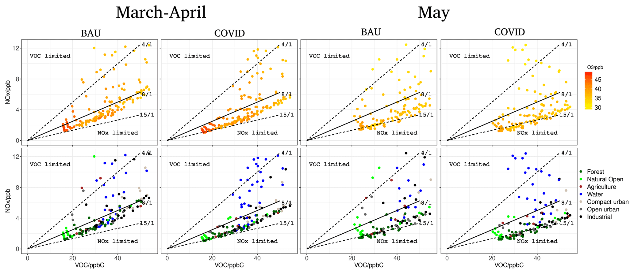
Figure 4 Modelled O₃ concentrations (top panels) for 30 March to 12 April (only weekdays) and for 18 to 30 May (only weekdays) for both simulations, BAU (left panels) and COVID (right panels), over the AMB area during the morning (06:00–08:00 UTC). Each dot of the top row corresponds to the O₃ concentration difference (ppb) of one grid cell of the AMB at the surface level. The dots in the lower row represent the land use for each model grid cell.

Figure 5 Same as Fig. 4 during the afternoon (13:00–15:00 UTC).

Figure 6 Same as Fig. 4 during the evening (19:00–21:00 UTC).

The differences between the BAU and COVID simulations for the second period (18 to 30 May) showed overall reductions in the NO₂ (−2 to −15 µg m⁻³, −10 % to −65 %) and VOC (up to −2 µg m⁻³, −16 %) levels, with high reductions found during the evening peaks (see Figs. S3 and S4). Ozone levels decreased (by up to 3.5 µg m⁻³; see Fig. S5) in most of Catalonia due to significant reductions in most of the emission sectors (see Fig. 3) during the COVID simulation, which decreased the high ozone productivity normally seen for this time of the year. However, we still found enhanced O₃ levels around the Barcelona airport in the evenings; the reductions in emission levels were still significant (more than 80 %; see Fig. 3) and inhibited titration of the O₃ by NO. Note that, in this case, the O_x concentrations decreased nearly everywhere in the Catalonia area and up to −4 µg m⁻³ over the AMB (see Fig. S6) for the COVID simulation, resulting in overall improvements in the air quality.

5 Discussion

5.1 O₃ sensitivity to precursors and land use

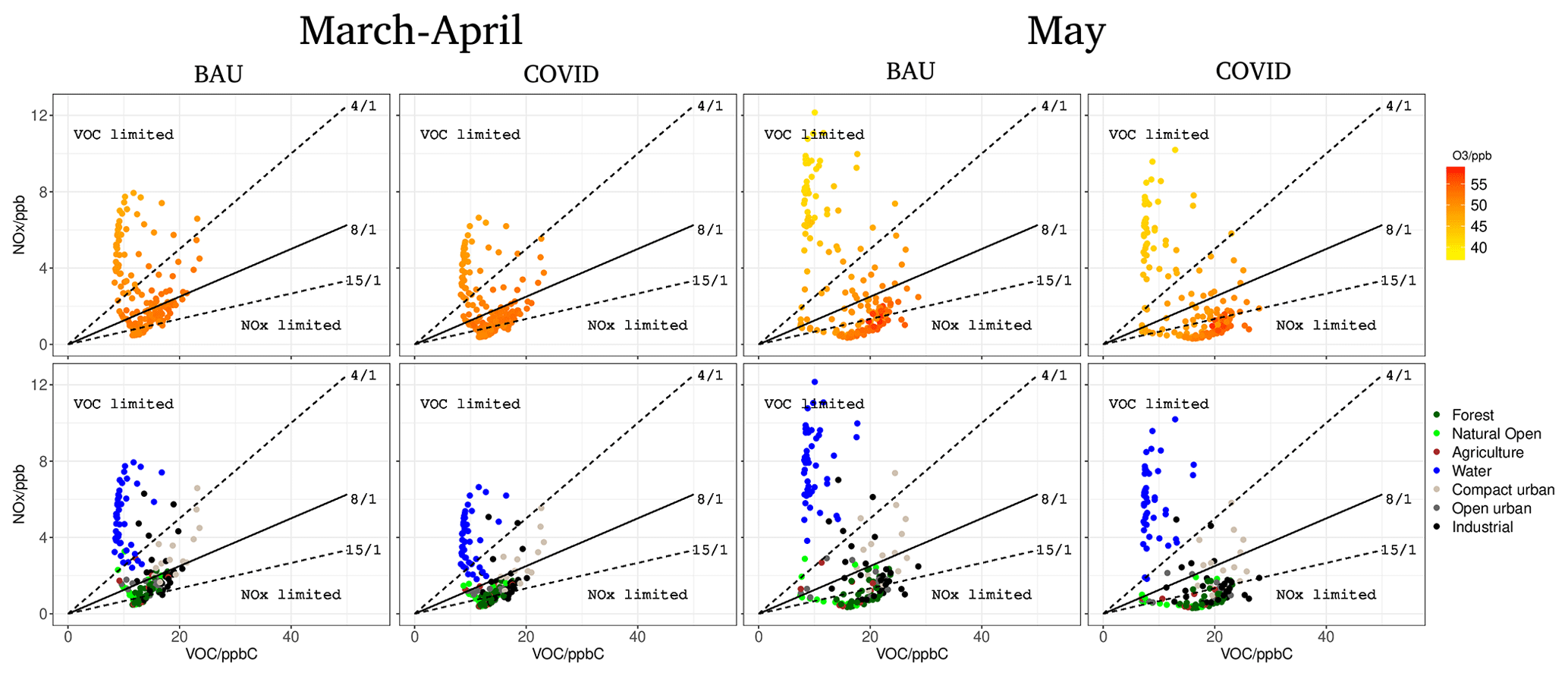
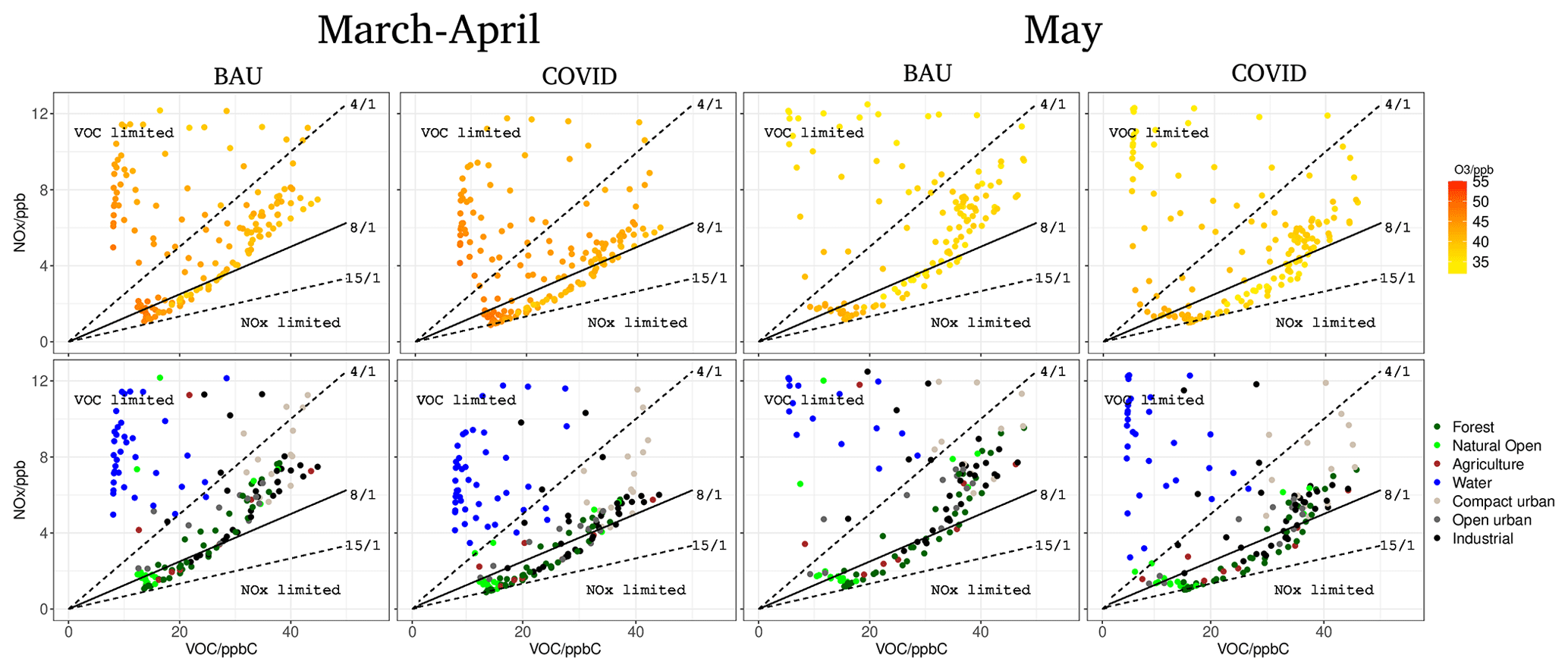
Variations in the levels of the O₃ precursors (NO_x and VOCs) had large effects on O₃ production. In addition, land use is the key to understanding how industrial, open urban, compact urban, water, agriculture, natural open, and forest land uses influenced the O₃ regimes (see Fig. S12 and Table S9 for more details on the land use classification). We represent this complex relationship in Figs. 4 (06:00 to 08:00 UTC), 5 (13:00 to 15:00 UTC), and 6 (19:00 to 21:00 UTC), which show the differences in surface NO_x, VOC, and O₃ concentrations in the BAU and COVID simulations during the first period (30 March to 12 April, only weekdays) and the second period (18 to 30 May, only weekdays). To complement this information, we calculated the average ${\mathrm{NO}}_{\mathit{\text{x}}}/\mathrm{VOC}$ ratios for these two periods in Table 3. Values of NO_x and VOC concentrations and relative changes for each land use are shown in Tables S7 and S8. In this study, we establish a relationship between surface VOC:NO_x and O₃ concentrations and, subsequently, derive the line separating the two different photochemical regimes by the local O₃ maximum (see Fig. S7). The local O₃ maximum occurs when VOC:NO_x ≈ 8 coincides with the ratio defined in National Research Council (1991). In Figs. 4–6, we indicate the NO_x-limited regime with a dark solid line separating VOC:NO_x >8, which is typical for locations located downwind of urban and suburban areas, and the VOC-limited regime (VOC:NO_x <8), which is typical for highly polluted urban areas (National Research Council, 1991). We also indicate the transitional regime with two dotted lines (VOC:NO_x $>\mathrm{4}/\mathrm{1}$ and VOC:NO_x $<\mathrm{15}/\mathrm{1}$) showing where ozone becomes less sensitive to NO_x changes and increases with increasing VOC levels, as identified in National Research Council (1991).

Overall, without any reduction in emissions (BAU simulation), this analysis indicates that in urban forests far from anthropogenic sources and influenced by high biogenic VOC emissions, the photochemical regime of O₃ formation is NO_x-sensitive in the mornings and afternoons. With the inland sea breeze fronts seen in the late afternoons and early evenings (Massagué et al., 2019), pollutants are transported from their sources (urban areas) to other areas (rural areas). Consequently, we found a transition to a VOC-limited regime in green areas (forest, natural open, and agriculture) in the evenings. Some of the grid points classified as naturally open and agriculture are close to the Barcelona airport (high NO_x sources), and the transport of pollutants (driven by the wind speed and direction) has a significant impact on their regime. However, we see that most of the grids classified as naturally open are NO_x-limited all day. In the case of grids classified as agriculture, we see that, in the morning and evening, most of these grids are in the transition or VOC-limited regimes, while in the afternoon, these grids are in the transition or NO_x-sensitive regimes. Areas close to highly polluted areas (including urban areas such as compact urban, industrial, and water) are in VOC-sensitive or transitional regimes all day, especially during the evening due to high traffic emissions. Note that “water points” are located around the harbour and the airport and are typically high NO_x sources. In terms of ozone levels (BAU simulation), high values during the morning (40–43 ppb) and evening (46–47 ppb) hours are found in suburban areas (forest and natural open) because there is less NO (because of less traffic) and thus less ozone degradation. In the afternoon, high O₃ levels are found everywhere in the AMB (49–55 ppb), especially in urban areas (industrial, open urban, and compact urban).

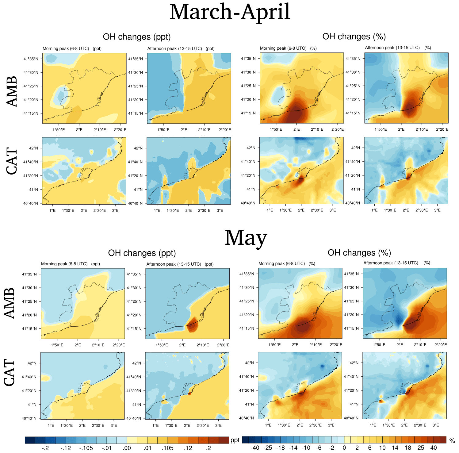
Figure 7 Morning and afternoon averaged surface OH changes over the metropolitan area of Barcelona (AMB) and the Catalonia region (CAT) during 30 March to 12 April (only weekdays) and 18 to 30 May (only weekdays), with absolute values (ppt) and relative changes (%) shown. Relative changes (%) were calculated as ((COVID − BAU) / BAU) × 100.

With the significant decrease in NO_x (20 %–40 %) and a slight decrease in VOC (1 %–10 %) levels during the lockdown (see Sect. 4.1), the averaged O₃ levels by land use increased for the COVID run (1 %–5 %), and chemical formation tends to enter the NO_x-sensitive regime, especially in the morning and afternoon hours during April–March. In the case of green areas (forest, natural open, and agriculture), we see clear transitions towards a NO_x-sensitivity regime. However, despite the cuts in emissions, most of the grids close to highly polluted areas (compact urban, industrial, and water) were still in the VOC-sensitive or transitional regimes all day, especially in the evenings (high traffic emissions), for which we found the highest ozone increases (2.4 %–5 %). Similar results were found when we compared both runs (BAU and COVID) for the period in May in terms of the changes in the chemicals for each land use. However, we found that, during May, the maximum ozone levels decreased in the COVID run during the afternoons (up to 1.6 % in green areas), which was attributed to reductions in the anthropogenic emissions that decreased the ozone precursor levels (24 % to 40 % for NO_x and 24 % to 40 % for VOCs) and consequently ozone production. For green areas far from anthropogenic sources (forests), the ozone levels were also reduced in the mornings and evenings during this period.

The lockdown measures inhibited NO titration of O₃, mainly due to changes in the local NO_x emissions resulting from road transport. This resulted in an increase in the O₃ levels during the evening hours, where there was no photolytic reaction with NO₂ in urban areas with high population densities. We found that air quality policies based solely on transport reduction (as illustrated by the COVID lockdowns, which reduced NO_x levels) actually intensified O₃ levels over urban areas, indicating the need for a protocol with strident control measures to reduce NO_x emissions without significantly reducing anthropogenic VOCs to control O₃ levels. However, high ozone production during May was reduced due to reduced levels of the precursors, and consequently there were reductions in the maximum ozone levels for that period.

5.2 Impacts on the atmospheric oxidation capacity

In addition to understanding changes in the levels of O₃ precursors, it is important to determine how emission changes affect the AOC, because this plays an important role in the loss and production rates of primary and secondary pollutants. The AOC is a good indicator of photochemical reactions, leading to the formation of secondary pollutants such as O₃ (Wang et al., 2022). We saw increases in the concentrations of the oxidants OH and NO₃ during the period March–April, mainly over the AMB, as shown in Figs. 7 and 8, where the left-hand-side panels indicate absolute concentrations (COVID − BAU) and the right-hand-side panels indicate relative changes in comparison to the BAU simulations ((COVID − BAU) / BAU × 100). OH is the dominant tropospheric daytime oxidant, and it increases considerably (up to 0.12 ppt, +45 %) because of significant reductions in NO₂ levels, since NO₂ is the primary OH sink (Elshorbany et al., 2009). The increase in these free radical concentrations could be the leading cause of the diurnal O₃ increases (see Fig. S5) given that VOC and CO oxidations by OH are the initial reactions for ozone formation. In addition, the NO₃ radical, which is a primary nighttime oxidant, also increases in areas close to the airport and harbour (4 ppt, 210 %). This increase can be explained by reductions in the VOC and NO₂ levels, which are important sinks for NO₃ radicals (Elshorbany et al., 2009; Saiz-Lopez et al., 2017).

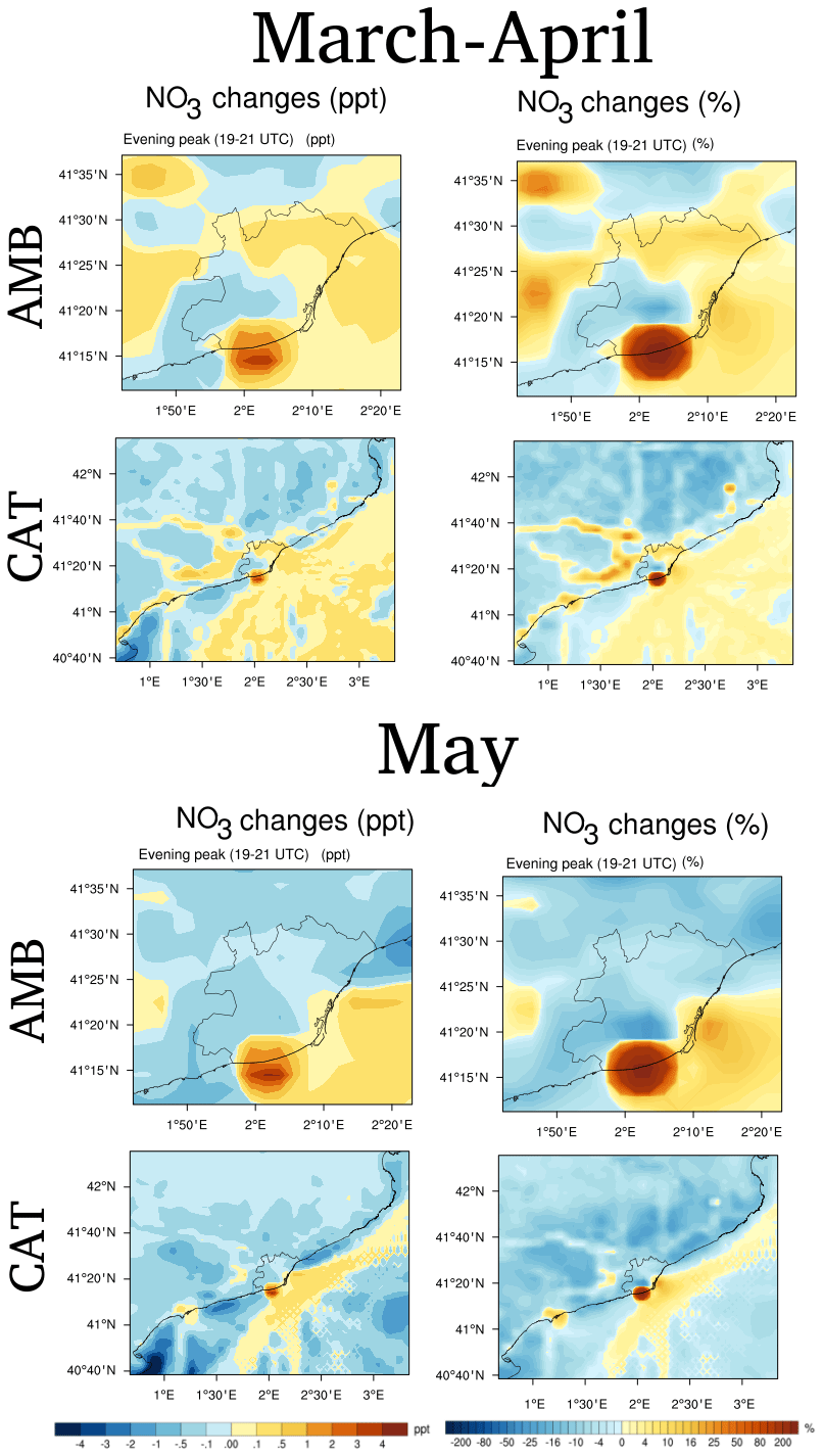
Figure 8 Evening-averaged surface NO₃ changes over AMB and CAT during 30 March to 12 April (only weekdays) and 18 to 30 May (only weekdays), with absolute values (ppt) and relative changes (%) shown. Relative changes (%) were calculated as ((COVID − BAU) / BAU) × 100.

During the period in May, we also found increases in the oxidant radicals (OH, NO₃) and also O₃ (see Fig. S5) of the COVID simulation with respect to the BAU in areas where substantial NO_x emission reduction took place, such as the airport and the harbour. In these areas, OH levels increase up to 0.3 ppt (55 %) in the afternoon, and NO₃ increases up to 4 ppt (230 %) in the evening. However, other areas showed general decreases in AOC radicals (−0.1 ppt for OH and −2 ppt for NO₃), resulting in decreases in the O₃ levels. Note that, for both periods, the decrease in shipping emissions (a source of NO_x) led to increases in the levels of both radicals along the ship tracks.

Our results indicate that changes in the anthropogenic emissions (mainly NO_x and VOCs) lead to significant changes in the OH and NO₃ radical levels, which in the case of emission reduction, such as that experienced during the COVID lockdown, leads to enhanced oxidation efficiency in the urban atmosphere of the AMB and O₃ enhancements. However, during the period in May, when O₃ formation increased due to warm temperatures and an increase in biogenic emissions, there was a decrease in the AOC (except in the airport and harbour areas) for the COVID run. The elevations of AOC occurred because these areas were still VOC-limited regimes during this period (see Sect. 5.1). In terms of air quality policy, it is important to understand the interplay between these free radicals and O₃ chemistry so that mitigation strategies are not counterproductive.

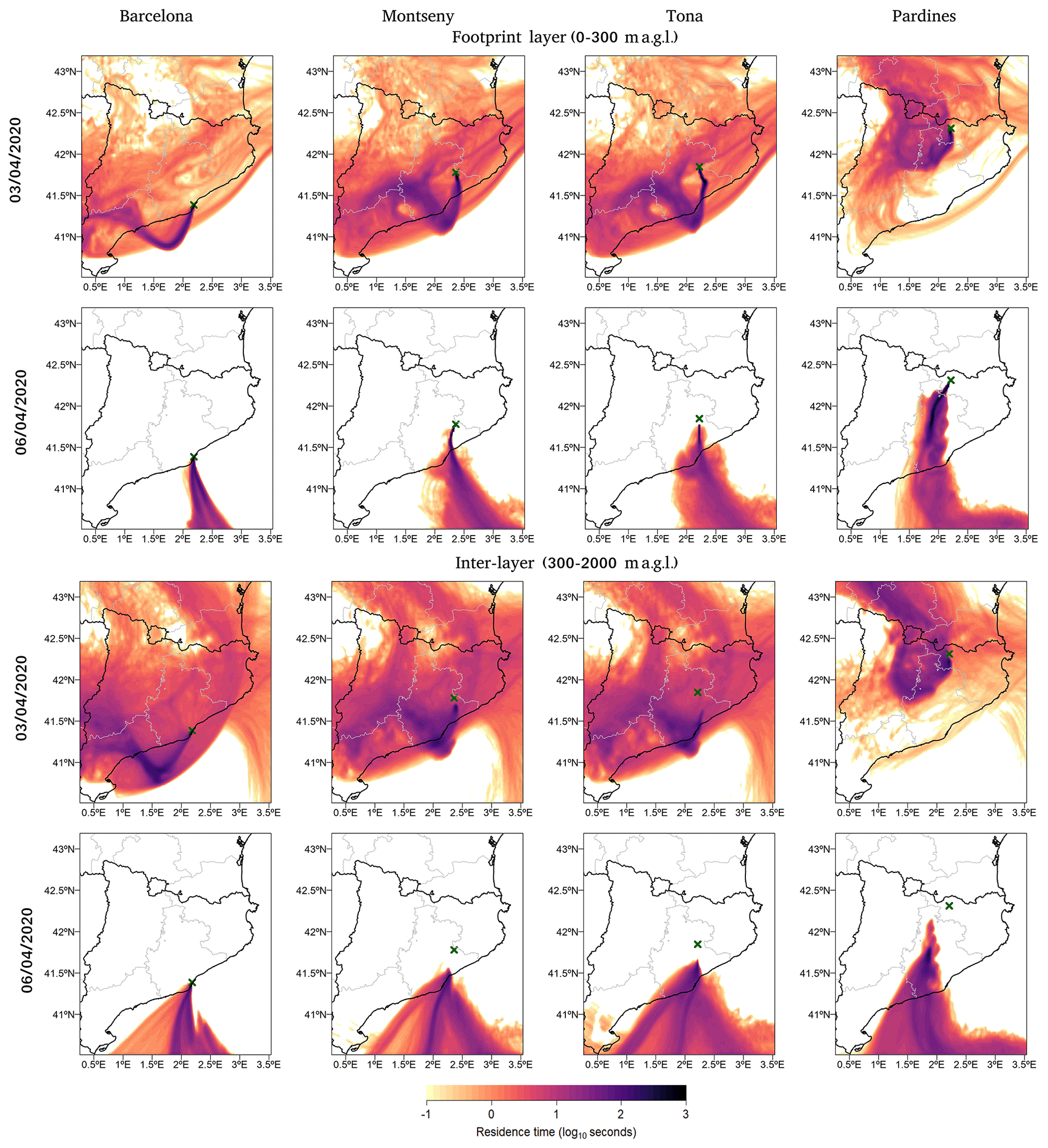
Figure 9 Simulated air parcel trajectories at the footprint layer (0–300 m a.g.l., top panels) and interlayer (300–2000 m a.g.l., bottom panels) for 3 and 6 April at 16 h at the four sites (from left to right): Barcelona, Montseny, Tona (Vic Plain), and Pardines. The location of each site is shown with a green cross.

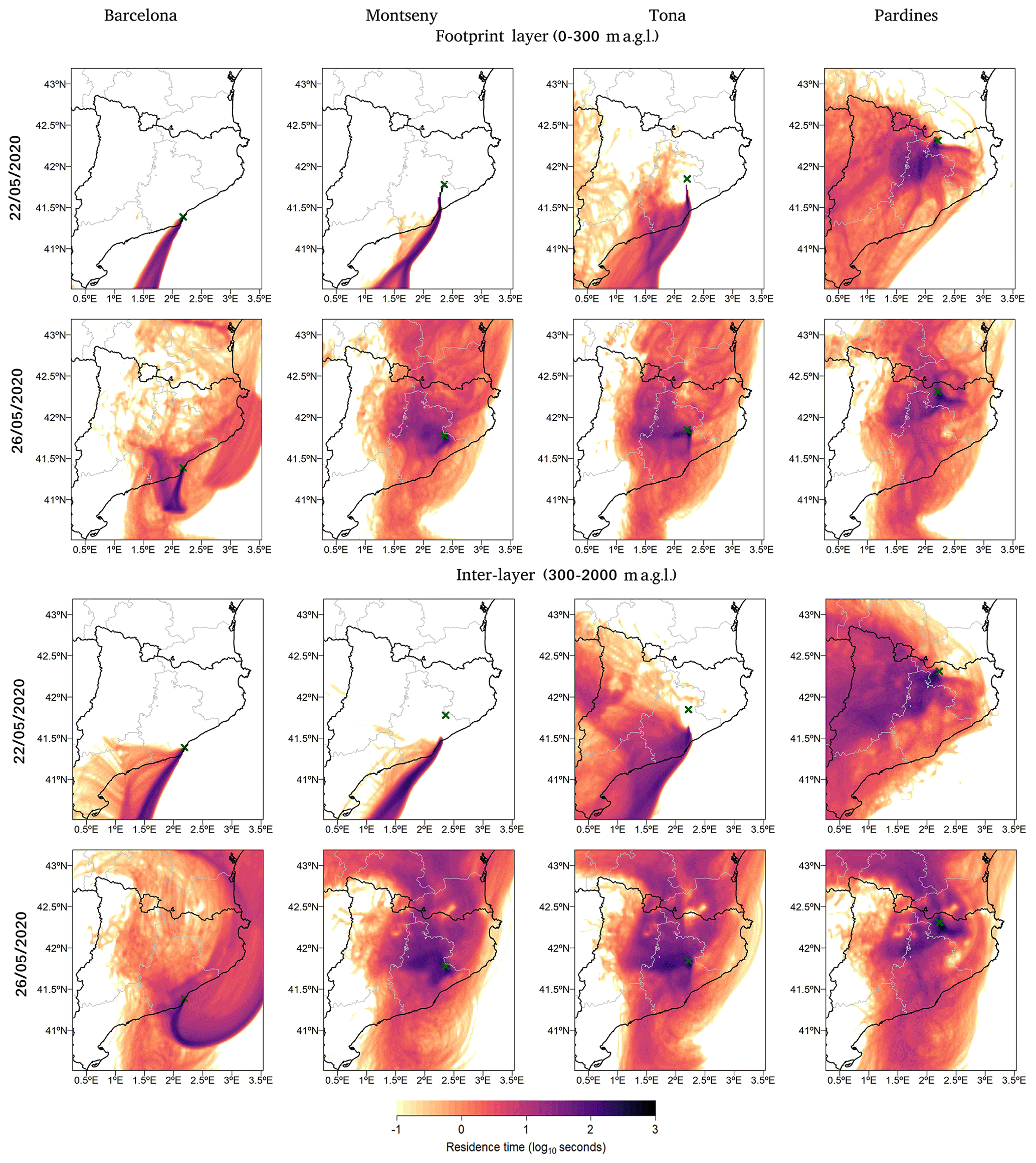
Figure 10 Same as Fig. 9 for 22 and 26 May. The location of each site is shown with a green cross.

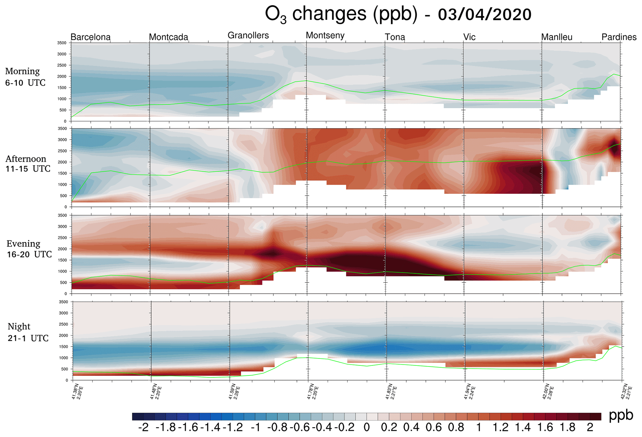
Figure 11 O₃ changes between the COVID and BAU simulations along the atmospheric plume from the AMB to the Pyrenees for 3 April. The modelled PBLH is shown with a green line.

5.3 Pollution transport from urban to rural

In addition to studying the mechanisms for ozone formation in the AMB, we explored how ozone is transported to rural areas to determine the influence of urban pollution. Rural areas far from the city, such as the Vic Plain and the Pyrenees mountain range, are frequently affected by the atmospheric plume transported northwards from the AMB (Massagué et al., 2019). Indeed, ozone exceedances over these places occur when there are high levels of NO₂ (mainly due to road traffic) over the AMB (see Sect. 2). The urban plume is driven inland by south-easterly and southerly combined sea–valley–mountain breeze winds channelled by north‒-south valleys, and it crosses the Catalan coastal and pre-coastal ranges to an intra-mountain plain.

Figure 12 Same as Fig. 11 for 6 April.

To understand how emission reductions in the AMB can affect the ozone levels in these rural areas, we analysed the differences in ozone concentrations between the COVID and BAU runs for 4 specific days (3 and 6 April from the lockdown period and 22 and 26 May from the relaxation period) during which the air masses flowed from the AMB northwards to the Pyrenees (as shown in Figs. 9 and 10) and generated high levels of O₃ pollution in the rural areas (see Table S1 and Figs. S8–S11). On 3 and 6 April there was no precipitation, with slightly high temperatures and low to moderate wind intensity, and on 22 and 26 May there was warm, sunny weather with anti-cyclonic conditions (see Table S2 for more information about the meteorological conditions). Figures 9 and 10 show the trajectories of the air masses arriving at the monitoring stations on the selected days: these were modelled with the Lagrangian FLEXible PARTicle dispersion model with WRF (FLEXPART-WRF) (Brioude et al., 2013). This version of the Lagrangian model works with the WRF mesoscale meteorological model, with the same parametrization as the WRF-Chem model (see Sect. 3.1). The transport model has been run in backwards mode, which means that what is represented in each plot is the residence time, at each grid cell of the map, for the air masses arriving at each site. Twenty-four-hour back-trajectories were calculated for each day at a release time of 16 h and with a grid cell size of 0.03 × 0.03 ^∘. Figures 9 and 10 show that the air masses on 3 April and 22 May were transported from the AMB to rural areas such as Montseny and the Vic Plain, and we can see an influence from the bottom layers (0–300 m) and the upper layers (300–2000 m) at the different sites. The air masses on 6 April were channelled from the AMB northwards to Montseny, the Vic Plain, and the Pyrenees. The air masses on 26 May were also transported from the AMB northwards to Montseny, the Vic Plain, and the Pyrenees, but the air masses that arrived at the surfaces of these locations had strong local components and larger influences from the upper layers.

Figure 13 Same as Fig. 11 for 22 May.

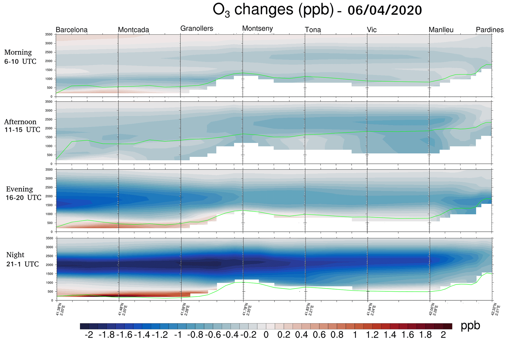
On 3 April, we found significant differences between the COVID and BAU runs during the afternoon and especially in the evening, when O₃ differences increased up to 2–3 ppb and higher enhancements were found over the Vic Plain (from the surface up to 2000 m), as shown in Fig. 11. High ground-level ozone concentrations over the Vic Plain could have been affected by vertical recirculation of the air mass with O₃ reservoirs from the upper layers (see Fig. S7) to the lower troposphere (Querol et al., 2017; Massagué et al., 2019). Later at night, ozone accumulated on the surface following a decrease in the planetary boundary layer height (PBLH), and it was removed by deposition and titration. However, the reduction in daytime NO_x emissions in the COVID simulations resulted in less titration capacity and consequently an increase in the ozone levels (1–2 ppb) that remained at the surface layer along the different sites on the S–N trajectory connecting the AMB, the Vic Plain, and the Pyrenees. For 6 April (Fig. 12), differences between the COVID and BAU runs were only found during the evenings and later in the nights, and the ozone levels increased in the COVID run (up to 2 ppb at the surface level) from the city of Barcelona to the mountain area of Montseny. On that day, this increase was not seen for the sites located farther north. Note that ozone decreases (1–2 ppb) were seen in the free troposphere, especially at night.

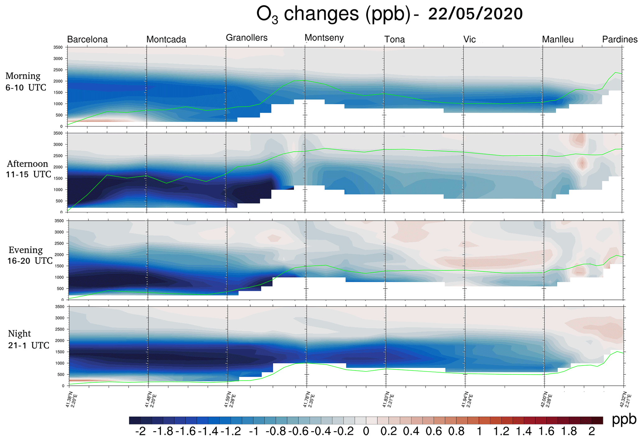
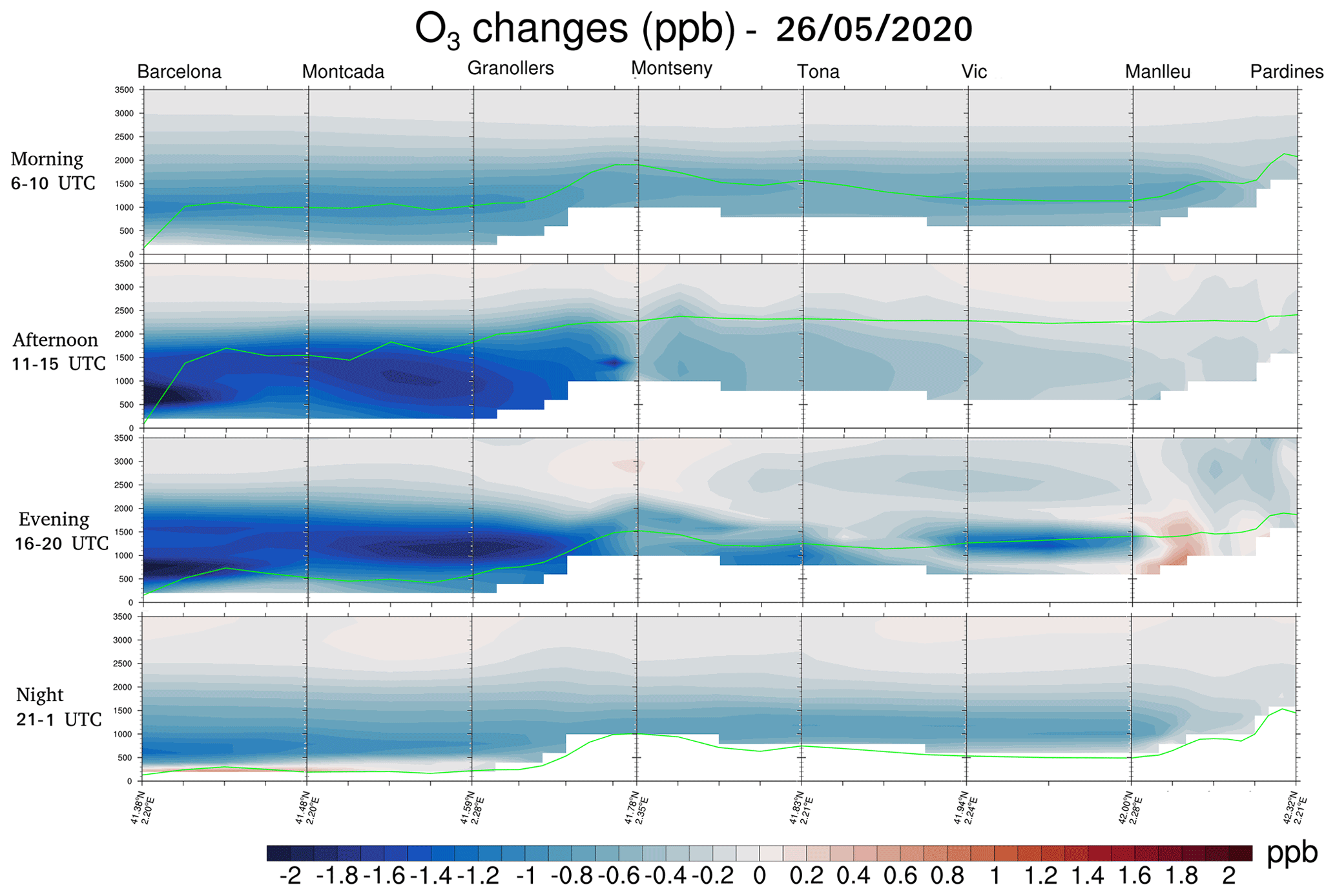
We found significant decreases in ozone levels in the COVID simulation (up to 3 ppb from the surface up to 2000 m) from the AMB north to the mountain area of Montseny on 22 and 26 May (Figs. 13 and 14, respectively), especially during the afternoons, when the PBLH was highest and solar radiation led to enhancement of the sea breeze front, which provided favourable conditions for regional transport (Massagué et al., 2019). The decreases in ozone precursor emissions (COVID simulation) resulted in less ozone production from the AMB plume and production of new O₃, and consequently the ozone concentrations decreased (discussed in Sects. 5.1 and 5.2). This decrease was also seen for the evening hours. Note that, at night, when ozone accumulated on the surface following the decrease in the PBLH, there was a slight increase in its levels due to limited titration by NO. However, there were still reductions in the ozone levels from 500 to 2000 m at night.

Our results showed that reduced ozone precursor levels increased the ozone levels during the evenings and nights in the COVID run due to reductions in the ozone titration process during the period of April–March, not only in urban areas, but also in rural areas such as Montseny, the Vic Plain, and the Pyrenees. During May, the emission reductions in the COVID simulation decreased the maximum ozone levels (in comparison with the BAU run) in the afternoon from the city of Barcelona to the mountain areas of Montseny, the Vic Plain, and the Pyrenees, thereby improving the air quality in all these areas. The improvement in the air quality is consistent with the decrease in surface O_x concentrations seen during the period of May over most of the Catalonia region (see Sect. 4.1).

A comparison of these two periods, April–March and May, showed that the mitigation strategies designed to reduce the high ozone levels were more efficient in May, when ozone formation was high (high biogenic emissions coinciding with anti-cyclonic conditions). Thus, given the importance of meteorology in air pollution events occurring over urban and rural areas, new mitigation strategies are needed to improve the air quality and would result in significant O₃ reductions: the local O₃ coming from the AMB plume would be reduced, as would the recirculated O₃ and thus the intensity of surface O₃ fumigation from high-O₃ reservoir layers in other areas.

Figure 14 Same as Fig. 11 for 26 May.

6 Conclusions

Improving air quality is a top priority in urban areas and requires a better understanding of how the O₃ levels respond to changes in the emission levels of the precursors, of the ozone formation regimes, and of the atmospheric oxidation capacity and the associated O₃ formation. Furthermore, urban emissions affect the O₃ levels in rural areas outside the cities. In this study, we used the WRF-Chem air quality model to analyse the air quality changes occurring over the metropolitan area of Barcelona and other (rural) areas affected by transport of the atmospheric plume from the AMB during mobility restrictions.

The large reduction in NO_x levels (up to 60 %) seen during the lockdown period combined with a slight change in VOC levels (up to 10 %) led to increased O₃ concentrations (up to 20 % in the evening). The significant increase found in the evening was mainly due to reduced O₃ titration by NO, which prevailed over the lower O₃ production level caused by decreases in the levels of the O₃ precursors. The lockdown occurred during April–March, when ozone photochemical production was still not at the highest level. In addition, our results showed a significant increase in the atmospheric oxidation capacity (AOC) indicated by the enhanced oxidant (OH and NO₃) levels, which was consistent with the slight increases seen in the maximum O₃ concentrations during the lockdown. We also found that, for several days, these increases were seen farther north in rural areas such as the Vic Plain, which produced the most annual exceedances in Spain. Large enhancements over these areas were the result of (1) a higher regional O₃ background level, (2) vertical recirculation of the air masses that transport high concentrations of O₃ from the upper levels to the lower levels, and (3) the contributions of the AMB pollution plume travelling along the S–N valley connecting the AMB, the Vic Plain, and the Pyrenees. High ozone levels seriously affect human health and the environment. In addition, the consistent differences seen in O_x (NO₂ + O₃) concentrations during the period April–March have important policy implications, i.e. that effective mitigation strategies designed to reduce air pollutants and their health effects should include reductions in both O_x and VOC levels to avoid increases in ozone levels.

During a period in May exhibiting high ozone production (high biogenic emissions and intense sunlight), decreases in the levels of the ozone precursors NO₂ and VOCs consequently decreased the maximum ozone (up to 4 µg m⁻³) and O_x (up to 4 µg m⁻³) concentrations seen over Catalonia. This was consistent with the unchanged or decreased AOCs given their strong link with O₃ production. For several days, this decrease in the ozone level was seen farther north in the rural areas. In this period, we also found ozone enhancements in the evening, mainly due to reduced O₃ titration by NO.

Furthermore, this analysis suggests that there was a tendency for both periods to move towards a NO_x-sensitive regime. However, some areas (open urban, compact urban, industrial, and water) were still under VOC-limited or transition regimes despite the remarkable NO_x reduction.

We propose that measures intended to reduce ozone precursor emissions (NO_x and VOC emissions) while maintaining stable O₃ formation levels in the AMB will result in important reductions in O₃ levels in both urban and rural areas, especially in the spring and summer, when the ozone productivity is highest. The current policies based on reducing transportation-related emissions alone could unintentionally increase the AOCs in and around large cities, thereby increasing the ozone levels. There is still a lack of research on relationships between AOC and ozone pollution. We also find that air quality policies must be designed in accordance with the $\mathrm{VOC}/{\mathrm{NO}}_{\mathit{\text{x}}}$ ratio, which dictates the O₃ sensitivity specific to a city. Furthermore, the significant effect of NO titration demonstrates the importance of defining mitigation strategies focused on VOC reductions. We also propose that more measurements of VOC levels are required to constrain the models representing these chemical processes, given the complexity of the relationship between these pollutants. In addition, the difficulty of models in simulating urban ozone precursors such as NO_x and VOC levels and, consequently, their link to the ozone chemistry should be addressed in future work to use the models as effective tools for assessing future studies aimed to reduce air quality.