the Creative Commons Attribution 4.0 License.
the Creative Commons Attribution 4.0 License.
 | 29 Jun 2022
A machine learning approach to quantify meteorological drivers of ozone pollution in China from 2015 to 2019
Grant L. Forster
Peer Nowack
Surface ozone concentrations increased in many regions of China from 2015 to 2019. While the central role of meteorology in modulating ozone pollution is widely acknowledged, its quantitative contribution remains highly uncertain. Here, we use a data-driven machine learning approach to assess the impacts of meteorology on surface ozone variations in China for the period 2015–2019, considering the months of highest ozone pollution from April to October. To quantify the importance of various meteorological driver variables, we apply nonlinear random forest regression (RFR) and linear ridge regression (RR) to learn about the relationship between meteorological variability and surface ozone in China, and contrast the results to those obtained with the widely used multiple linear regression (MLR) and stepwise MLR. We show that RFR outperforms the three linear methods when predicting ozone using local meteorological predictor variables, as evident from its higher coefficients of determination (R2) with observations (0.5–0.6 across China) when compared to the linear methods (typically R2 = 0.4–0.5). This refers to the importance of nonlinear relationships between local meteorological factors and ozone, which are not captured by linear regression algorithms. In addition, we find that including nonlocal meteorological predictors can further improve the modelling skill of RR, particularly for southern China where the averaged R2 increases from 0.47 to 0.6. Moreover, this improved RR shows a higher averaged meteorological contribution to the increased trend of ozone pollution in that region, pointing towards an elevated importance of large-scale meteorological phenomena for ozone pollution in southern China. Overall, RFR and RR are in close agreement concerning the leading meteorological drivers behind regional ozone pollution. In line with expectations, our analysis underlines that hot and dry weather conditions with high sunlight intensity are strongly related to high ozone pollution across China, thus further validating our novel approach. In contrast to previous studies, we also highlight surface solar radiation as a key meteorological variable to be considered in future analyses. By comparing our meteorology based predictions with observed ozone values between 2015 and 2019, we estimate that almost half of the 2015–2019 ozone trends across China might have been caused by meteorological variability. These insights are of particular importance given possible increases in the frequency and intensity of weather extremes such as heatwaves under climate change.
- Article
(6497 KB) - Full-text XML
-
Supplement
(1473 KB) - BibTeX
- EndNote


Over the last decade, Chinese policymakers have been successfully implementing air pollution control policies and strategies, such as The Clean Air Action Plan in 2013 (Chinese State Council, 2013), to reduce harmful air pollutants. As a result, annual mean concentrations of fine particulate matter (PM2.5) have been reduced by 30 % to 50 % from 2013 to 2018 in China (Zhai et al., 2019), alongside significant decreases in anthropogenic emissions of air pollutants and ozone precursors such as nitrogen oxides (NOx) and carbon monoxide (CO) with 21 % and 23 % reductions, respectively, from 2013 to 2017 (Zheng et al., 2018). However, summertime means of maximum daily 8 h average (MDA8) surface ozone concentrations were still increasing from 2013 to 2019 at a rate of about 1.9 ppb yr−1 on average across China, with a faster rate of 3.3 ppb yr−1 in the North China Plain (NCP) (Li et al., 2020), highlighting the urgent need for a better understanding of how ozone pollution could be addressed effectively.
Surface ozone is an air pollutant that can induce severe harm to both human health and ecosystems (Lefohn et al., 2018; Lelieveld et al., 2015). In the troposphere, it is primarily produced through photochemically induced reaction chains involving volatile organic compounds (VOCs), NOx and CO (Monks et al., 2015; Jacob, 2000). It is well-known that the effectiveness of ozone production is strongly dependent on the atmospheric chemical regime (e.g. Squire et al., 2015; Archibald et al., 2020), in which ozone production is mainly controlled by the abundance of NOx or VOCs. Many urban and industrial regions in China have been identified and categorized as being within the VOC-limited regime (Ou et al., 2016; Wang et al., 2017). Under these circumstances, surface ozone reductions may require tighter controls on emissions of VOCs together with continuous reductions in NOx, while significant reductions in NOx emissions without simultaneous and adequate controls on VOCs could lead to increased ozone pollution in the short term (Wang et al., 2019). Notably, the total emissions of non-methane volatile organic compounds (NMVOCs) have actually increased by 11 % in 2017 compared to 2010 (Zheng et al., 2018). Another factor might be the role of the large reductions in PM2.5, especially during the period 2013–2017, because fewer particles could reduce the aerosol sink of ozone-producing radicals such as hydroperoxyl (HO2) (Li et al., 2019a). However, the quantitative contribution to the increases of ozone from HO2 uptake on aerosol remains uncertain (e.g. Tan et al., 2020), and it is likely that this effect has become less important as PM2.5 concentrations continue to decline (X. Chen et al., 2021; Li et al., 2019b).
In conjunction with the effects of changing ozone precursor emissions, the effect of meteorological conditions on ozone concentrations should always be considered. It is well-known that ozone variations are strongly co-determined by meteorological factors such as incoming solar radiation, temperature, humidity, atmospheric stagnation and precipitation (e.g. Otero et al., 2018; Zhang et al., 2018; Lu et al., 2019a). For example, solar radiation is pivotal to the photochemical production and destruction of ozone (Finlayson-Pitts and Pitts, 2000). Higher surface temperatures, and in general tropospheric temperatures, change the chemical reaction rate of many ozone-relevant chemical reactions and will affect biogenic emissions of VOCs such as isoprene and monoterpenes which are also important ozone precursors (Lu et al., 2019a; Doherty et al., 2013; Guenther et al., 1993; Xie et al., 2008; Archibald et al., 2020). Work by Lu et al. (2019b) further indicated that hotter and drier weather conditions were the main drivers for background ozone increases in 2017 in major city clusters of China. Similarly, Ma et al. (2019) suggested that high biogenic emissions of VOCs and meteorological conditions indicative of heatwaves such as high temperature, low wind speed and no precipitation can elevate ozone pollution in NCP. Furthermore, studies by Wang et al. (2021) and Pu et al. (2017) also found enhanced ozone concentrations during heatwaves in the Pearl River Delta (PRD) and Yangtze River Delta (YRD). Such links between meteorology and ozone pollution provide clear evidence for the necessity to quantify the influence of meteorological factors or even climate change on ozone pollution in China (e.g. Lu et al., 2019a; Meehl et al., 2018). Characterizing the major meteorological drivers behind ozone variations in different regions of China will also be crucial for achieving effective mitigation of ozone pollution now and under future changes in climate.
To quantify the importance of meteorological drivers, previous studies such as Li et al. (2019a) and Han et al. (2020) adopted stepwise multiple linear regression (MLR) to derive linear relationships between meteorological factors and measured surface ozone concentrations across China. Both of these studies demonstrated the significant skill of stepwise MLR in modelling ozone and in quantifying the driver–response relationships. Nevertheless, a key limitation of stepwise MLR or conventional MLR is that these methods are not able to accurately capture nonlinearity, which is a severe constraint given that nonlinear relationships between meteorological factors and ozone, e.g. between temperature and ozone, are to be expected (e.g. Pu et al., 2017; Gu et al., 2020; Archibald et al., 2020). In addition, MLR can suffer from a severe loss in predictive skill and reliability in settings where a large number of (collinear) meteorological factors are considered as predictors (cf. the curse of dimensionality in high-dimensional regression problems; Nowack et al., 2021; Bishop, 2006). Although the stepwise MLR approach adopted by Li et al. (2019a) can overcome collinearity and overfitting to some extent (i.e. because only a few predictors that are particularly strongly influencing ozone concentrations are kept), it is inevitable that many relevant meteorological factors will be excluded from the final MLR predictions using such an approach.
In order to capture any nonlinear relationships between many meteorological factors and ozone and to overcome the potential limitations of considering collinearity and high-dimensional settings in MLR, we will use a machine learning approach as the next logical step to advance such controlling factor analyses of ozone pollution. Specifically, we will adopt random forest regression (RFR) (e.g. Grange et al., 2018; Stirnberg et al., 2021) as a nonlinear approach and contrast the results to a linear statistical learning approach that is also robust in high-dimensional settings in the form of ridge regression (RR) (e.g. Nowack et al., 2018). Both RFR and RR will also be compared with more conventional statistical methods such as MLR and stepwise MLR.
Our paper is structured as follows: in Sect. 2, we describe the data used in this study and the modelling framework of the two machine learning algorithms, namely RFR and RR. In Sect. 3, the performances of RFR and RR will be discussed first and then compared to those achieved with MLR and stepwise MLR. We then summarize the most important meteorological drivers for surface ozone as identified by RFR and RR. Finally, we conduct a trend analysis of recent surface ozone changes in China, and use our method to estimate the contribution of meteorological effects.
2.1 Surface ozone and meteorological data
The surface air quality measurement data used in this study were obtained from https://quotsoft.net/air/ (last access: 13 July 2021; Wang, 2021) which is a mirror of the data from the Ministry of Ecology and Environment (MEE) in China. For the purposes of quantifying ozone pollution severity, we use the maximum daily 8 h rolling mean (i.e. MDA8) of ozone calculated following the guidelines by the Ministry of Environmental Protection of the People's Republic of China (MEP, 2013). The calculation selects the maximum value from the 8 h rolling mean of ozone for each station between local time (UTC+8 h) 08:00 and 24:00 on each day. To be considered, each station must have a valid 14 h data record of 8 h rolling mean of ozone within 08:00 to 24:00 on a respective day, otherwise, the MDA8 ozone is not calculated for that day. Previous studies (e.g. Li et al., 2020, 2019a; Han et al., 2020) have focused on ozone pollution during the boreal summer months, i.e. June, July and August (JJA), as the season with the most frequent occurrence of extreme ozone episodes in China. In this work, we extend the analysis period to include the months from April to October to account for the fact that the seasonality of ozone does not follow a uniform pattern across China. For example, peak ozone concentrations are often found during autumn in the PRD region (Gao et al., 2020; see Fig. S1 in the Supplement). In addition, we further constrain our analysis to the period 2015–2019 to maintain greater consistency of the ozone data throughout our analysis period as the MEE included far fewer measurement stations prior to 2015. In order to maintain consistency and reliability of all ozone data from stations within the study period, only those stations with more than 80 % temporal coverage of MDA8 ozone data record in each year are selected. For quality assurance of the data, we further examined each station's MDA8 ozone variation individually and noticed that measurements from some stations appeared to show a less reliable data record than others. This was for example evident from extended periods of non-fluctuating ozone levels (see Fig. S2), or from sudden unusual MDA8 spikes, usually followed by periods of suppressed ozone variability (see Fig. S3). According to our best judgement, such abrupt changes or unrealistically low variability are unlikely to reflect actual ozone pollution profiles. Data from stations that showed such unusual time evolutions were excluded from our analysis to avoid the inclusion of unrealistic artefacts. The list of stations not used in this study is summarized in Table S1 in the Supplement.
To study regional meteorological drivers of ozone, we distinguish four regions of particularly high population density known as Beijing–Tianjin–Hebei (BTH), Yangtze River Delta (YRD), Pearl River Delta (PRD) and Sichuan Basin (Sichuan), with definitions frequently used in previous studies (e.g. Li et al., 2019a; Han et al., 2020). The boundaries of these four regions are adjusted to ensure that stations in each region have similar topography and equivalent elevation. The four regions are also known as the target areas for air pollution reduction in Chinese government plans (MEE; http://www.mee.gov.cn/hjzl/dqhj/cskqzlzkyb/, last access: 1 December 2021; Li et al., 2019a). The locations of stations within the four regions are indicated by red dots in Fig. 1.
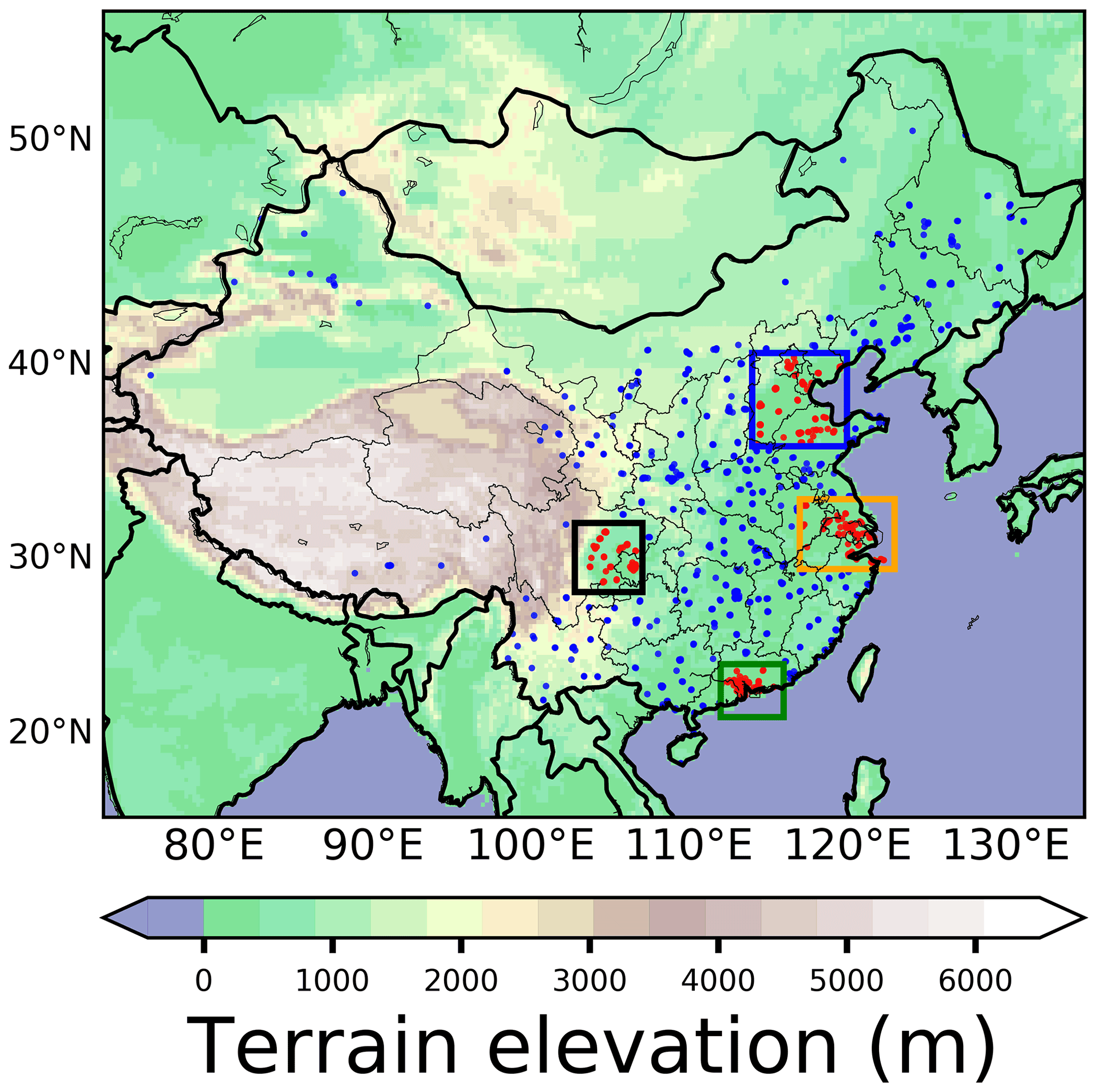
Figure 1Elevation height (m) and locations of all ground-based stations and the four megacity cluster regions, BTH (blue box; 114–120∘ E, 36–40.62∘ N), YRD (orange box; 117–123∘ E, 29.458–33.238∘ N), PRD (green box; 112–116∘ E, 21–24.111∘ N), Sichuan (black box; 102.8–107.061∘ E, 28.2–31.976∘ N). Red (blue) dots indicate the locations of stations within (outside) the four regions.
For the meteorological data, we use the gridded ERA5 reanalysis product (Hersbach et al., 2020) available at https://cds.climate.copernicus.eu/ (last access: 11 November 2021). Specifically, we use hourly data for a total of 11 meteorological variables at 0.25∘ × 0.25∘ spatial resolution, namely the temperature at 2 m (T2), boundary layer height (BLH), mean sea level pressure (SLP), surface solar radiation downward (SSRD), relative humidity (RH) at 1000 hPa, total precipitation (TP), zonal wind at 10 m (U10), meridional wind at 10 m (V10), zonal wind at 850 hPa (U850hPa), meridional wind at 850 hPa (V850hPa) and vertical velocity at 850 hPa (W850hPa) for the same time period as for the ozone station data. Then the MDA8 ozone data are spatially averaged within the dimensions of each ERA5 grid cell to obtain the best possible spatial match between the station-based ozone data and the large-scale meteorological factor data.
The variables of T2, BLH, SLP, RH, TP, U10 and V10 can also be found as predictors in the controlling factor analyses from the studies of Han et al. (2020) and Li et al. (2019a). The SSRD is included in this study instead of adding a cloud coverage term as done by Han et al. (2020) and Li et al. (2019a). Essentially, we consider SSRD to more directly characterize the local photochemical environment for ozone production and loss than cloud coverage. Zonal and meridional wind at 10 m may be important for the dispersion of ozone's precursors on a local scale. Both zonal and meridional winds at 850 hPa are adopted in this study in order to encompass the effect of transport of more polluted or cleaner air from remote regions. Wind at 850 hPa is less likely to be affected by orography than wind at 10 m altitude, and it is thus better suited for considering the effect of larger-scale transport and dispersion. Additionally, we represent the role of vertical transport of air masses by including vertical velocity at 850 hPa as another factor.
2.2 Data pre-processing
Prior to modelling ozone, we pre-processed the meteorological data by averaging the raw hourly data over different periods each day and this process is summarized in Table 1. The averaging periods were not the same for all meteorological variables. For example, T2, SSRD, SLP, RH and W850hPa are averaged between local time (UTC+8 h) 06:00 to 18:00 each day. The average of these hours is sufficient to cover all daytime hours when ozone is photochemically produced from April to October. Total precipitation is calculated by summing up all hourly accumulated precipitation (m) from 06:00 to 18:00. For zonal and meridional wind at 10 m and 850 hPa, data are averaged over 06:00 to 12:00, which covers the main hours that may have potential fresh emission of precursors and transport or dispersion of precursors or ozone. The BLH is averaged over 00:00 to 12:00 for the consideration of both potential night-time emission of industrial activities when the boundary layer is still low and transportation emission during morning rush hours. Through this process, raw hourly meteorological data can be converted to a daily format, temporally matching MDA8 ozone data. Finally, both ozone data and meteorological data are deseasonalized. Specifically, for MDA8 ozone and the converted daily meteorological variables, we first calculate 15 d moving window averages centred on the particular calendar date from 2015 to 2019. We then take the difference between each day's MDA8 ozone or daily meteorological variables and these 15 d averages to obtain daily anomalies, creating smooth time series of deseasonalized MDA8 ozone and deseasonalized meteorological variables.
Table 1Summary of the meteorological controlling factor variables and the respective times of day considered in their averages. The motivation behind each selected time period is provided in the main text. Note: a positive zonal wind means westerly; positive meridional wind means southerly; positive vertical velocity means downward motion.
2.3 Machine learning methods for modelling MDA8 ozone
To model the relationships between meteorological variables and MDA8 ozone concentrations in China, we use two regression algorithms, a nonlinear approach, RFR and a linear approach, RR. Within our framework, the predictors are the deseasonalized meteorological variables from ERA5 and the dependent variable is the deseasonalized ground-based MDA8 ozone. For RR, both the deseasonalized meteorological variables and the deseasonalized ozone time series are standard-scaled (normalized to zero mean and unit standard deviation) to avoid an imbalance of factors in the regularization part of the RR cost function (Nowack et al., 2018).
Both RFR and RR have been extensively described elsewhere (e.g. Nowack et al., 2018; Grange et al., 2018; Mansfield et al., 2020; Nowack et al., 2021) and it is beyond the scope of this study to provide an in-depth description. Briefly, RFR is based on learning an ensemble of decision trees, where each individual tree splits data into groups until reaching certain pre-set definitions for data “purity” (Breiman, 2001; Grange et al., 2018). The RR is a least-squares linear regression method augmented by L2-regularization aiming to avoid overfitting in high-dimensional regression settings, especially in regression problems with strong collinearity (McDonald, 2009). Both RFR and RR are known to handle collinearity comparatively well (e.g. Dormann et al., 2013), which is key given that many meteorological variables such as temperature and solar radiation are correlated with each other. To assess whether these two machine learning algorithms can improve the accuracy of ozone modelling compared to conventional statistical methods, we will contrast our results to MLR, which may not be highly capable of handling collinearity and overfitting, and stepwise MLR. For MLR, we simply adopt the same modelling framework of RFR and RR; all 11 meteorological variables are ingested into MLR as predictors. For stepwise MLR, we adopted a similar approach as Li et al. (2019a): we start with 11 deseasonalized meteorological variables as predictors in MLR and remove one predictor at a time, based on the smallest significance of the regression coefficient in each new subset of predictors, until there are only three meteorological predictors left. These three predictors are considered to be important predictors and are used in the final model of stepwise MLR for modelling deseasonalized MDA8 ozone.
2.4 Training, testing and cross-validation in machine learning
Supervised machine learning approaches such as the two algorithms we use here require distinct training, validation and testing phases to tune the relevant hyperparameters (explained in detail below) and to validate the skill of the resulting predictive functions on new, unseen data not used in the training and tuning process (e.g. Bishop, 2006). During the training phase, both predictors (i.e. deseasonalized meteorological variables) and dependent variables (i.e. deseasonalized MDA8 ozone) are available and each machine learning regression algorithm is fit to this dataset, assuming different combinations of values for the hyperparameters of each algorithm. The best objective estimate for the combination of hyperparameters is then found in the validation step by predicting ozone values for a validation dataset not used at the training stage (e.g. for a different year in the data record). During the testing phase, the trained and validated algorithm is used operationally to make new predictions for ozone values given a new dataset for the meteorological variables as input to the machine learning function. These test set predictions can then be used to measure the out-of-sample skill of the algorithm in predicting ozone pollution given certain meteorological conditions. In this study, we split the 5 years of data (2015–2019) systematically into training/validation and testing datasets, one at a time and in a rotating fashion. Specifically, 4 of these 5 years are classified as training/validation data, leaving 1 year for testing. To ensure that we are measuring the true predictive performance and relationships, our predictive results and model evaluations are only conducted for the test data, which has not been used at the training and validation stages. This process rotates until ozone data for each year have been assigned once as test data so that all 5 years of data can be predicted by RFR and RR.
Machine learning regressions such as RFR and RR optimize their predictive performance by tuning certain sets of hyperparameters. To determine the most suitable set of hyperparameters, we use a statistical cross-validation method. Specifically, the 4-year training/validation set is further split into four folds (1 year per fold). We then run a grid search over pre-defined combinations of hyperparameters by training on three folds and predicting on the fourth fold in a classic four-fold cross-validation procedure. We finally select the best-estimated set of hyperparameters on the basis of the average validation data prediction performance as measured by the coefficient of determination, i.e. the R2 regression score function, which is one of the metrics used in Scikit-learn (see https://scikit-learn.org/stable/modules/generated/sklearn.metrics.r2_score.html, last access: 13 April 2022; Scikit-learn, 2022), and refit model coefficients using this set of hyperparameters for the entire 4 years of training/validation data. We note that we avoid a “leave-one-out” cross-validation method (in which only one daily sample is the test dataset at a time) as we expect autocorrelation in our data (i.e. MDA8 ozone may share similarity in adjacent dates), which, intuitively, could lead to an overestimate of our predictive skill if testing data immediately follow training data points.
The ranges of hyperparameters we search over for both RFR and RR are set as follows: for RFR, the maximum depth for trees growing is iterated in a step of 1 from 8 to 15. The maximum percentage of features and maximum samples (with the bootstrap method) is set from 20 % to 90 % and 30 % to 80 % with 10 % incremental steps, respectively. The total tree number for the forest is set at 200 as a compromise between model complexity and runtime. Optimizations further showed that the minimum samples per leaf are best set to three in our RFRs so that we finally kept this value constant in our grid searches. In terms of RR, the regularization strength is iterated over a range of 1 to 199 with an incremental step of 2, which appeared to encapsulate the best solution in each case. A detailed explanation of these hyperparameters for RFR and RR is provided in Nowack et al. (2021).
2.5 Identifying and quantifying importance of meteorological drivers
Both RFR and RR can enable the identification of the most important meteorological drivers for MDA8 ozone and can help to quantitatively evaluate their relative importance. For RFR, we measure the importance of each meteorological predictor through a metric called Gini importance. A greater Gini importance implies a greater influence of a particular predictor (i.e. the deseasonalized meteorological variable) on the dependent variable (i.e. deseasonalized MDA8 ozone) (e.g. Menze et al., 2009; Zhao et al., 2019; Kuhn-Régnier et al., 2021). Since we train the RFR five times given each possible set of 4-year training/validation data, we average the Gini importance scores for each meteorological predictor across all five runs for our final discussion below. For RR, similar to MLR, the importance of each predictor is evaluated by the magnitude of each predictor's averaged slope (linear regression coefficient) across all 4-year training/validation datasets, which represents the linear effect of each predictor on ozone, given that all predictors are standard-scaled (see Sect. 2.3).
3.1 Machine learning performances for modelling ozone using local meteorological predictors
It is important to first assess how well the selected machine learning algorithms can model ozone by using only meteorological variables as predictors. Therefore, we adopt the coefficient of determination (R2) as a standard metric for the evaluation of prediction performance, which assesses the goodness of fit for the linear regression between the deseasonalized MDA8 ozone data and the predicted values (e.g. Han et al., 2020). As mentioned above, to measure the true predictive skill of the machine learning functions, we only compare our predictions for out-of-sample test data that are not used during training/validation stages against the deseasonalized measured MDA8 ozone data.
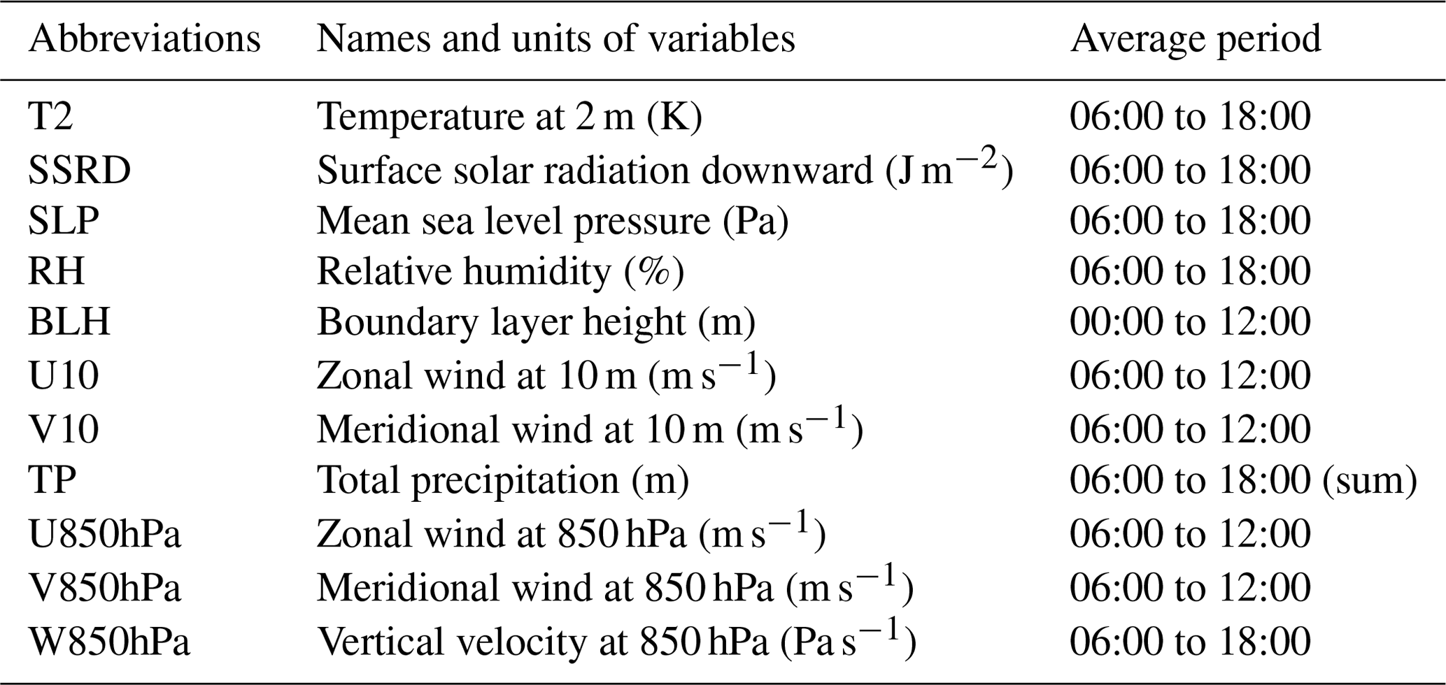
To begin with, the predictors used by RFR and RR are only the local meteorological variables; i.e. each ERA5 grid point's meteorological variables are used as predictors to model the averaged deseasonalized MDA8 ozone for that particular grid location. The average prediction performance of RFR and RR, by comparing predictions across all test years against the deseasonalized measured MDA8 ozone data across China, is illustrated in Fig. 2.
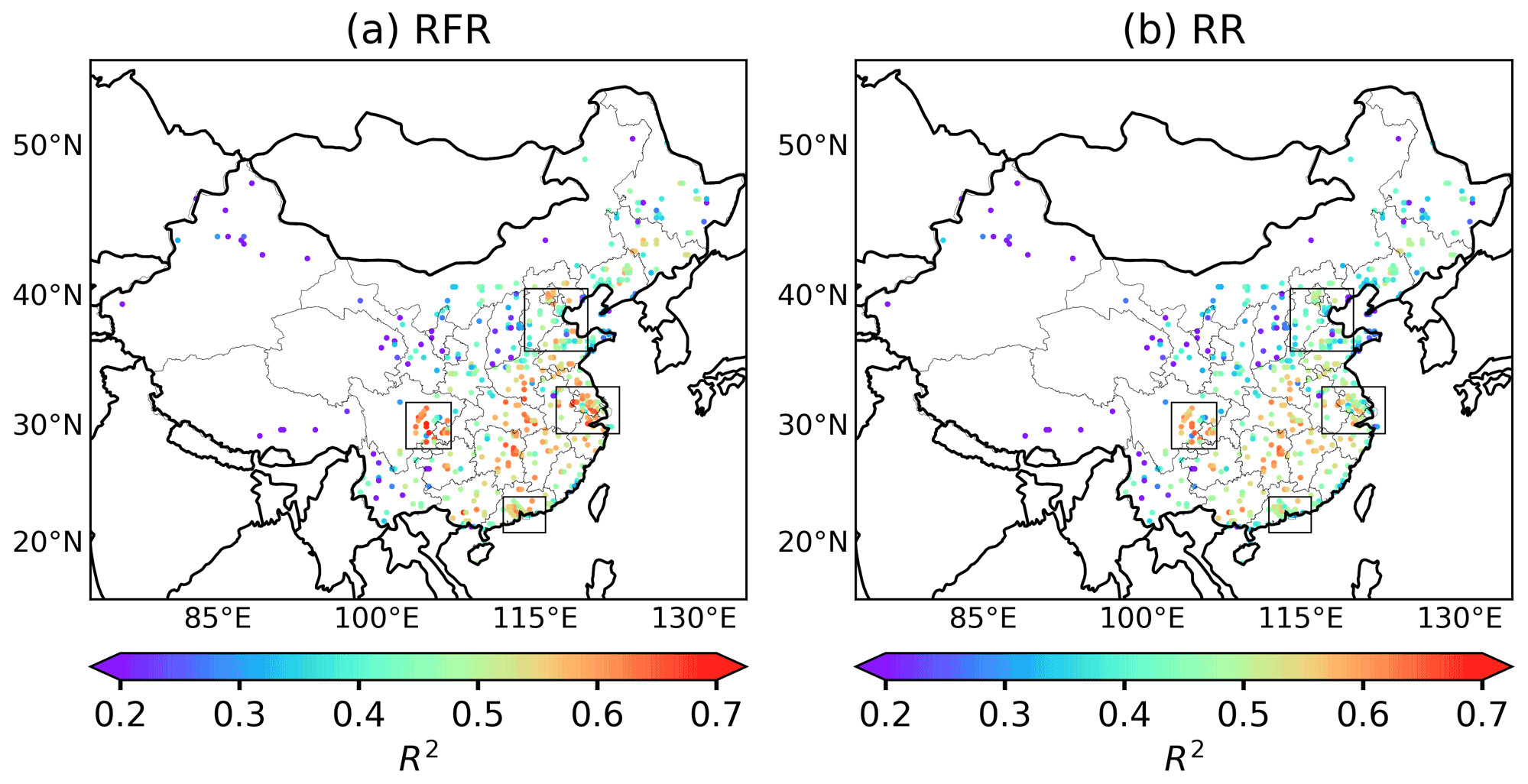
Figure 2Coefficient of determination (R2) between deseasonalized observational MDA8 ozone and deseasonalized predicted values in random forest regression (RFR) (a) and ridge regression (RR) (b). The skill is only measured for the respective test datasets. Each dot represents the centre of the ERA5 grid location, within which station values for MDA8 ozone are averaged.
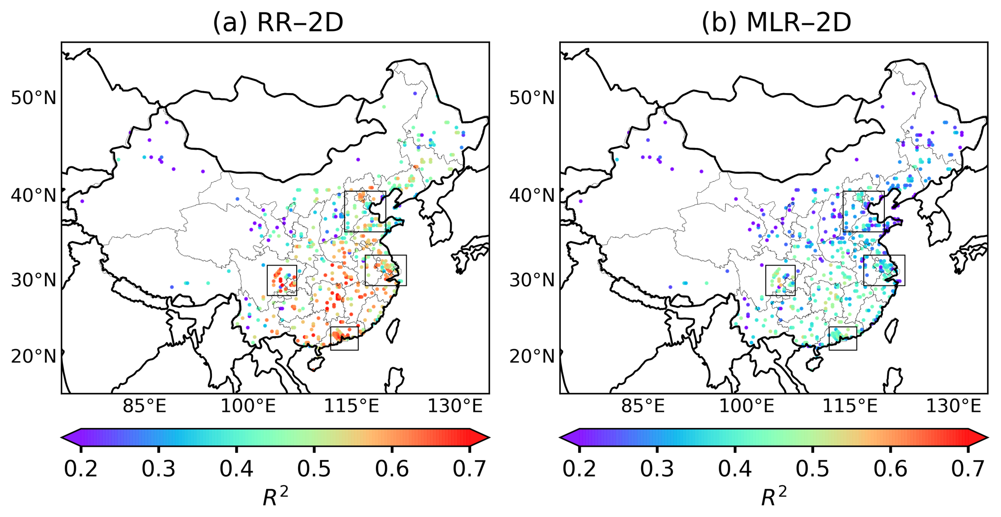
Figure 3Coefficient of determination (R2) between deseasonalized observational MDA8 ozone and deseasonalized predicted values of MDA8 ozone in ridge regression (RR) with 2D expansion (a) and MLR with 2D expansion (b).
Overall, the model performance of RFR generally surpasses the one of RR over most regions of China, with higher R2 values in grid locations within Sichuan, YRD, PRD and other regions of southeast China. The R2 values for RFR generally range from 0.5 to 0.6 across China while RR reaches R2 values from 0.4 to 0.5. Both RFR and RR perform similarly over the central region of BTH, while in the northern region of BTH (e.g. Beijing), R2 values are still found to be higher in RFR than RR. The averaged R2 across all ERA5 grid locations within BTH, YRD, PRD and Sichuan is 0.46, 0.56, 0.53 and 0.57, respectively for RFR, which are all higher than the equivalent R2 for RR (BTH: 0.41, YRD: 0.48, PRD: 0.47, Sichuan: 0.53).
In order to examine whether RR can improve the model performance by addressing overfitting, we also applied MLR with all 11 meteorological predictors and the stepwise MLR approach with the three most important meteorological factors in the final MLR for comparison. Although most R2 values across China for these three linear regressions (i.e. RR, MLR and stepwise MLR) are within the same range of 0.4 to 0.5, stepwise MLR shows the worst performance with consistently lower R2 values across China, and more of these values fall in a lower range of 0.3 to 0.4. Moreover, the averaged R2 values for stepwise MLR in BTH, YRD, PRD and Sichuan are found to be lower at 0.39, 0.45, 0.43 and 0.52, respectively (see Fig. S4b for the spatial distribution of R2 values). This suggests that the stepwise MLR approach may carry a risk of not including all important meteorological predictors in the regression model. However, RR does not show noticeable improvements over MLR, as evident from similar regionally averaged R2 values (see Table 2 and Fig. S4a), suggesting that the problem of collinearity is still limited given the use of 11 meteorological predictors. The enhanced performance of RFR compared to RR may therefore be attributed to the ability of RFR to model nonlinear relationships between local meteorological variables and ozone, indicating that a flexible machine learning approach, such as RFR that can capture nonlinearity, is more suitable to reflect relationships between local meteorological factors and ozone.
3.2 Predictive skill using additional nonlocal meteorological predictors
Weather systems that affect ozone (e.g. high-pressure systems) usually consider large spatial domains, driving regional temperature anomalies and suppressing or accelerating airflow in certain directions. Consequently, it seems intuitive that a meteorological controlling factor framework for ozone might benefit from including additional nonlocal information in the regressions, i.e. if we were to consider surrounding meteorological context information that is not just limited to the predicted ozone grid point in question (Ceppi and Nowack, 2021).
We thus ran a second version of our controlling factor analysis to investigate the spatially wider effect that meteorology may have on a two-dimensional (2D) domain of meteorological variables. This is possible since both RR and RFR better address collinearity and overfitting in high-dimensional regression settings than simple non-regularized MLR approaches, meaning that the additional information included in the regressions might well outweigh the cost of adding more predictors.
In detail, for each ozone target grid point, we include a meteorological context by adding each meteorological variable within a 7.5∘ × 7.5∘ rectangular domain around the centre of this target grid point to the set of model predictors, i.e. all the meteorological variables from the ERA5 0.25∘ × 0.25∘ grids within this 7.5∘ × 7.5∘ rectangular domain are used as individual predictors in the regression models. This adds potentially important information about the larger-scale meteorological situation to our predictions, but also significantly increases the dimensionality (number of predictors) of our regression problem and increases the number of collinear predictors. Indeed, we find that through the additional L2-regularization in RR with 2D expansion (denoted as RR–2D), its predictions by far outperform its MLR–2D equivalent, which now suffers from severe overfitting (compare R2 values in Fig. 3a and b). Noteworthy, with the increase of dimensionality in RR–2D, the regularization strength now is adjusted to larger values starting from 103 to 109 with a factor of 1.42 incremental increase at each step, which is much higher than the regularization strength set in RR with only local predictors. Such a large increase in range is due to the consideration of adding a large number of meteorological predictors within the 2D domain, and it ensures that the best solution with the most suitable regularization strength for each run can be well covered within this range. The overall R2 values for RR–2D range from 0.5 to 0.6 while R2 in MLR–2D ranges from 0.3 to 0.4; MLR–2D is overall worse than MLR with only local meteorological predictors in terms of R2. It is well-known that RFR may not be as effective at handling multi-collinearity in very high-dimensional settings as RR (e.g. Dormann et al., 2013) and its training time also increases exponentially with the number of predictors. We thus only ran RFR with 2D expansion (denoted as RFR–2D) for the southern Chinese PRD region, where we found a particularly large R2-value improvement after including nonlocal predictors in RR–2D (R2=0.60) as compared to local RR (R2=0.47), and even nonlinear local RFR (R2=0.53). These results highlight the apparent importance of large-scale meteorological phenomena in this region. However, we find that RFR–2D improves the average R2 value (0.57) relative to RR and RFR with only local predictors, but does not perform better than RR–2D.
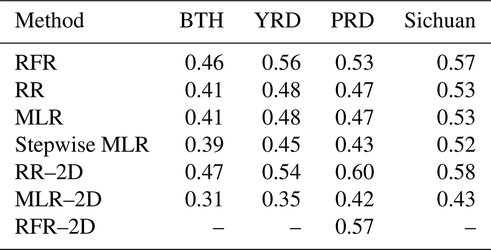
For clarity, Table 2 summarizes the averaged R2 in each region by all machine learning methods including RFR, RR, MLR, stepwise MLR, RR–2D, MLR–2D and RFR–2D. In summary, RFR and RR–2D are overall the two machine learning algorithms with the highest R2 in these four regions, while MLR and RR are equivalent.
Table 2Averaged R2 in the four regions by different machine learning algorithms, namely RFR, RR, MLR and stepwise MLR with only local meteorological predictors, RR–2D, MLR–2D with additional two-dimensional (2D) nonlocal meteorological variables and RFR–2D which is only conducted for the PRD region. In general, with only local meteorological variables, RFR performs the best with the highest averaged R2 in four regions. RR–2D and RFR–2D show improvement over the PRD region compared to RFR.
3.3 Regionally averaged prediction skill
In order to assess the performance of the algorithms in modelling the regional average ozone, we further compared our regionally averaged machine learning predictions by RFR, RR and RR–2D against observations for each of the four selected regions in China (Fig. 4), whereas previously we compared regional averages based on predictions for individual grid points whose R2 values were subsequently averaged within each region. For this purpose, we averaged all 0.25∘ × 0.25∘ grid point observations and model results within each region first and then compared the resulting time series for each test dataset directly. The results for each region are shown in Fig. 4, where the goal for the predictions is to fall as close as possible to the 1 : 1 line, in combination with a high R2 value (coefficient of determination). With only local meteorological predictors, RFR still outperforms RR regarding both R2 and slope (closer to 1) in all four regions. This can likely be attributed to the ability of RFR to capture nonlinearity as well.
Using this calculation method, the regional R2 values are much higher. For RFR, regional R2 in BTH, YRD, PRD and Sichuan are 0.71, 0.75, 0.7 and 0.83, respectively. The higher values can be partially explained by the fact that individual grid points are more prone to the effect of local emissions and related local uncertainties, whereas larger regional averages can smooth out some of these local effects. For instance, stations that are located relatively close to an emission source may be more influenced by the NOx-titration effect which may lower ozone levels (Sillman, 1999). This effect can be more significant in some urban areas (Li et al., 2017) or stations affected by fresh emissions of NOx from power plants (X. Zhang et al., 2021). Nearby emission of precursors may also be the dominant factor in driving ozone changes in regular weather conditions. Ozone production in these stations may be less sensitive to meteorological drivers but more influenced by local emissions.
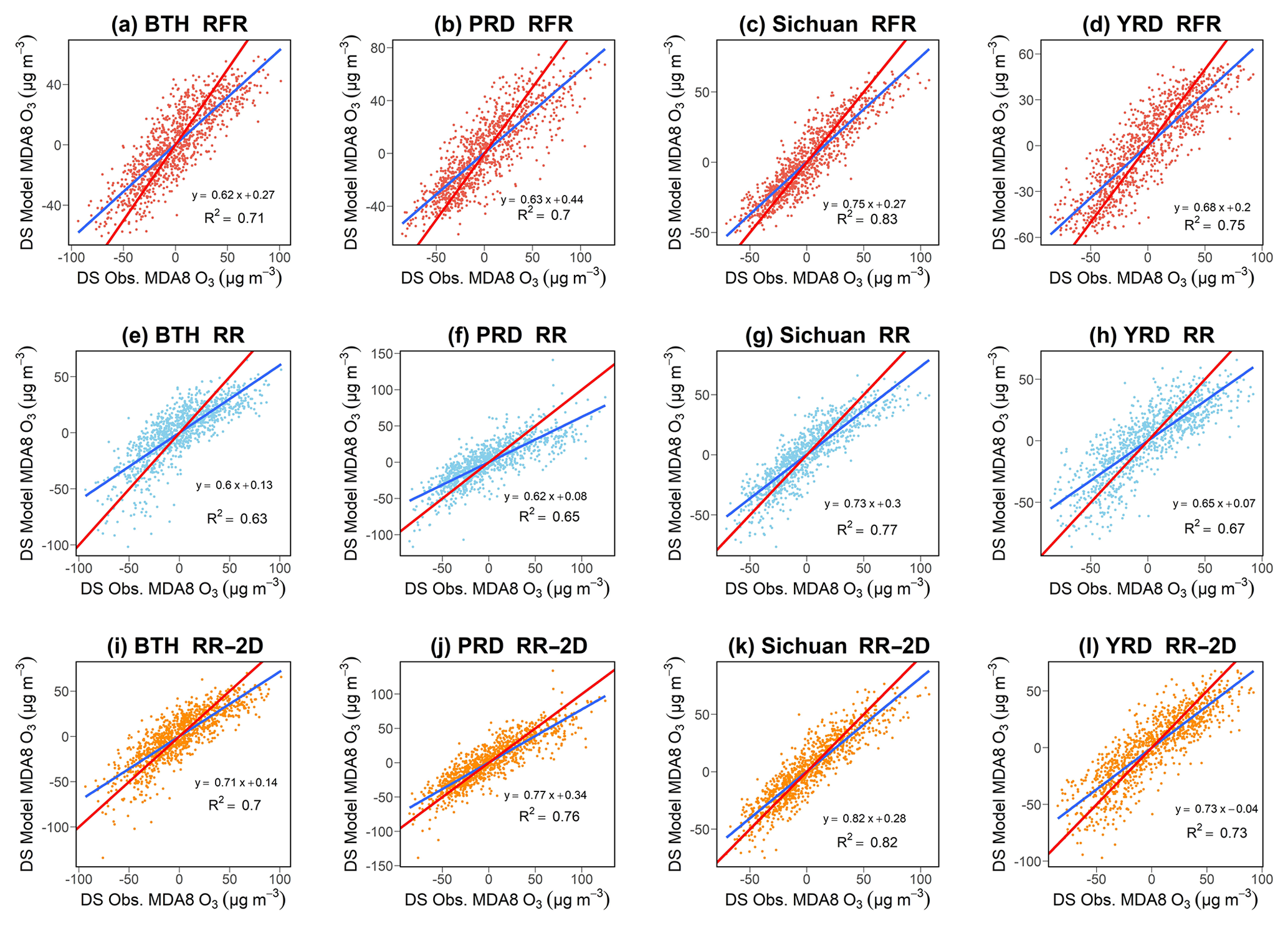
Figure 4(a–d) Comparison of regional averages of deseasonalized MDA8 ozone between model predictions and observations for RFR, (e–h) RR and (i–l) RR–2D. Linear fits between predicted and observed data are indicated by blue lines; red lines are the ideal 1 : 1 lines. The values for both models and observations are averaged over all ERA5 grid points in each region. Each graph contains information of the linear regression with slope and R2 value (coefficient of determination).
In summary, all machine learning methods show high skill in modelling meteorologically driven ozone variability. However, similar to results by Han et al. (2020), all linear fits of predicted versus observed ozone values in all regions for both RFR and RR have slopes lower than 1, suggesting a systemic underprediction of ozone for the highest observed ozone levels (higher than the deseasonalized zero mean) and overpredictions of ozone for low ozone pollution regimes (lower than the deseasonalized zero mean). As previously mentioned, such a mismatch may – at least to a degree – arise from non-meteorological factors such as the effect of precursor emissions, which are not taken into account here given the assumption that certain but not all emissions are related to the meteorological factors. Although regionally averaged prediction skill is less affected by local emissions, it will not be completely free from such effects. The increase of the magnitude of the slopes in RR–2D (closer to 1) also suggests that considering nonlocal meteorological variables may help improve the performance of ozone pollution controlling factor analyses, even if nonlinearity is not intrinsically taken into account.
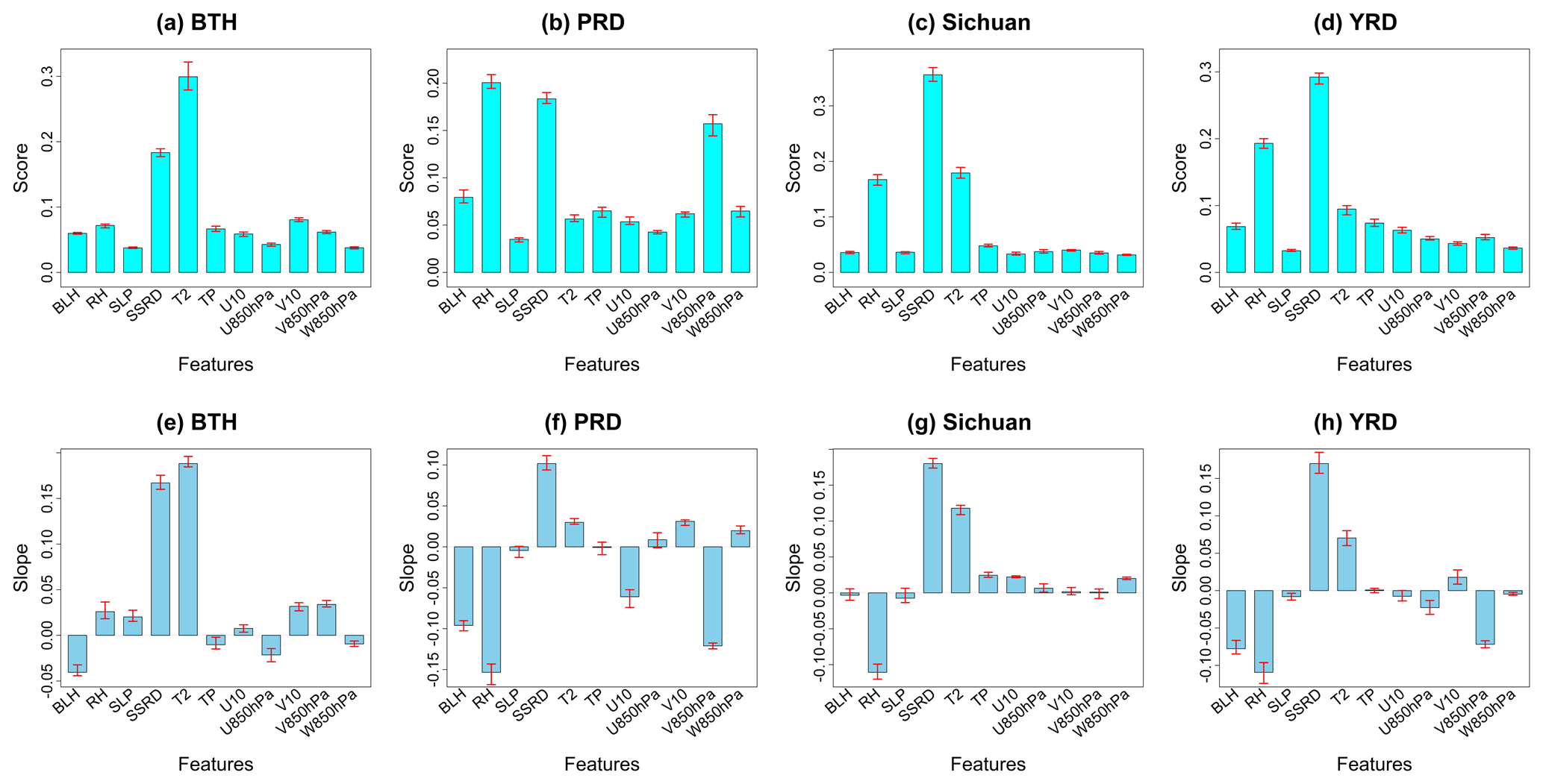
Figure 5(a–d) Average Gini feature importance scores of each meteorological variable for RFR in each region. (e–h) Average slopes of each meteorological variable for RR in each region. The red bars indicate the range of importance scores/slopes found across the five regression models learned to predict the left-out test years.
3.4 Quantifying the importance of meteorological predictors
We next aim to quantify how important each local meteorological predictor is for ozone pollution across China. For RR, we use the regression slope as a standard metric to measure how important each of the meteorological predictors are on ozone pollution. A large positive value for the slope (regression coefficient) of a meteorological predictor indicates that the predictor has a strong positive effect on ozone levels and vice versa. Since each set of 4-year training data are learned from independently, we will show averaged results. For RFR, we measure each predictor's importance through Gini importance (see Sect. 2.5). The highest absolute value for both the RR slope or RFR Gini importance is interpreted as the most important meteorological driver variable identified through our data-driven learning procedure. Note that Gini importance only allows measuring relative influences of predictor variables on ozone variability, but not the sign of the influence, i.e. a high value of Gini importance score is not able to determine whether the predictor has a positive or negative effect on ozone.
The Gini importance scores estimated by RFR and the slopes learned by RR for each region are shown in Fig. 5. Both Gini importance scores and slopes are initially estimated for every ERA5 grid location within each region and then averaged across the entire region and across all five learned regression functions.
In general, both RFR and RR show good agreement in terms of identifying the dominant meteorological drivers for each region. The temperature at 2 m is found to be the most important meteorological driver for ozone in BTH, followed by SSRD, albeit the relative difference between these two variables differs more clearly for RFR, which might be caused by nonlinearity in the ozone–temperature relationship (Fig. S5). Temperature was also identified as the most important meteorological variable in BTH by Li et al. (2019a) using MLR. Moreover, a more pronounced positive correlation between daily maximum temperature and MDA8 ozone is found in northern regions of China (Fig. 6a), which is consistent with the findings of these two machine learning algorithms. Since temperature is identified as the key meteorological factor in BTH, more severe ozone pollution with increasing temperature is expected and may be caused by increased rates of chemical kinetics for ozone's production (e.g. Lu et al., 2019a), the contribution of biogenic emissions (e.g. Ma et al., 2019) and anthropogenic emissions such as solvent evaporation which may be intensified in hot weather (e.g. Song et al., 2019; Qi et al., 2017).
For both YRD and Sichuan, surface solar radiation is the most important determinant of ozone variations, with RR slopes again indicating the expected positive relationship between sunny, clear-sky days and high ozone pollution. Furthermore, surface solar radiation is found to be central in BTH and PRD by RFR and RR. Given that Li et al. (2019a, 2020) and Han et al. (2020) did not consider this meteorological variable in their analyses, we recommend that it could be used more generally in the future. High solar radiation stimulates the photochemical environment, which has been suggested as one of the key mechanisms in YRD by Pu et al. (2017). From a large-scale meteorological point of view, such clear-sky conditions in YRD that may enhance severe ozone pollution in this region may be modulated by the western Pacific subtropical high (WPSH) (Shu et al., 2016; Chang et al., 2019; Shu et al., 2020). In the Sichuan, with complex terrain that can complicate atmospheric circulation, ozone pollution is often associated with the occurrence of high-pressure systems associated with clear-sky conditions and high temperatures (Ning et al., 2020), which is also identified by both RFR and RR.
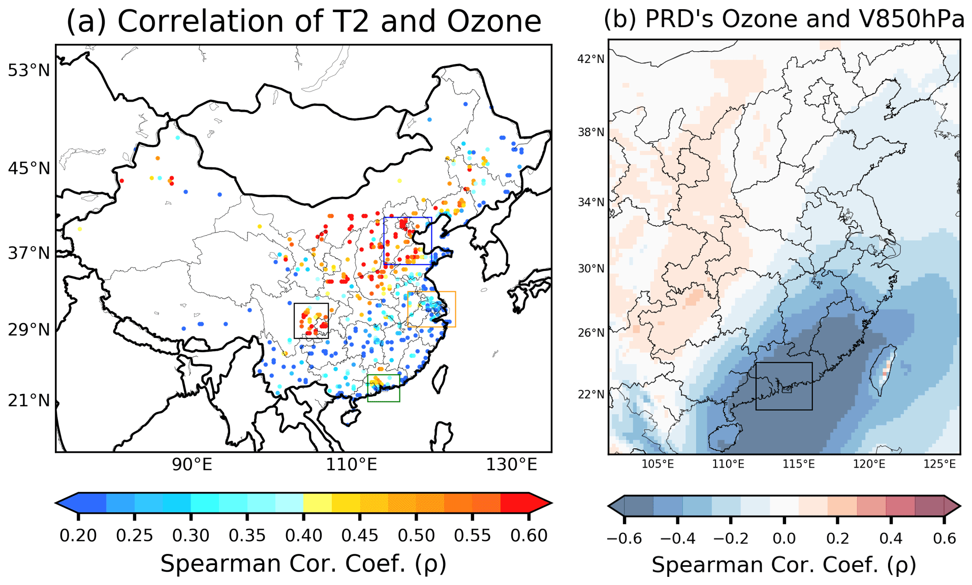
Figure 6(a) Spearman correlation between daytime (06:00 to 18:00) averaged temperature at 2 m and MDA8 ozone from 2015 to 2019 from April to October. (b) Correlation coefficients between the regional average of MDA8 ozone in PRD and the daytime (06:00 to 12:00) meridional wind at 850 hPa at each ERA5 grid point from April to October of 2015 to 2019. A positive value of meridional wind indicates southerly wind.
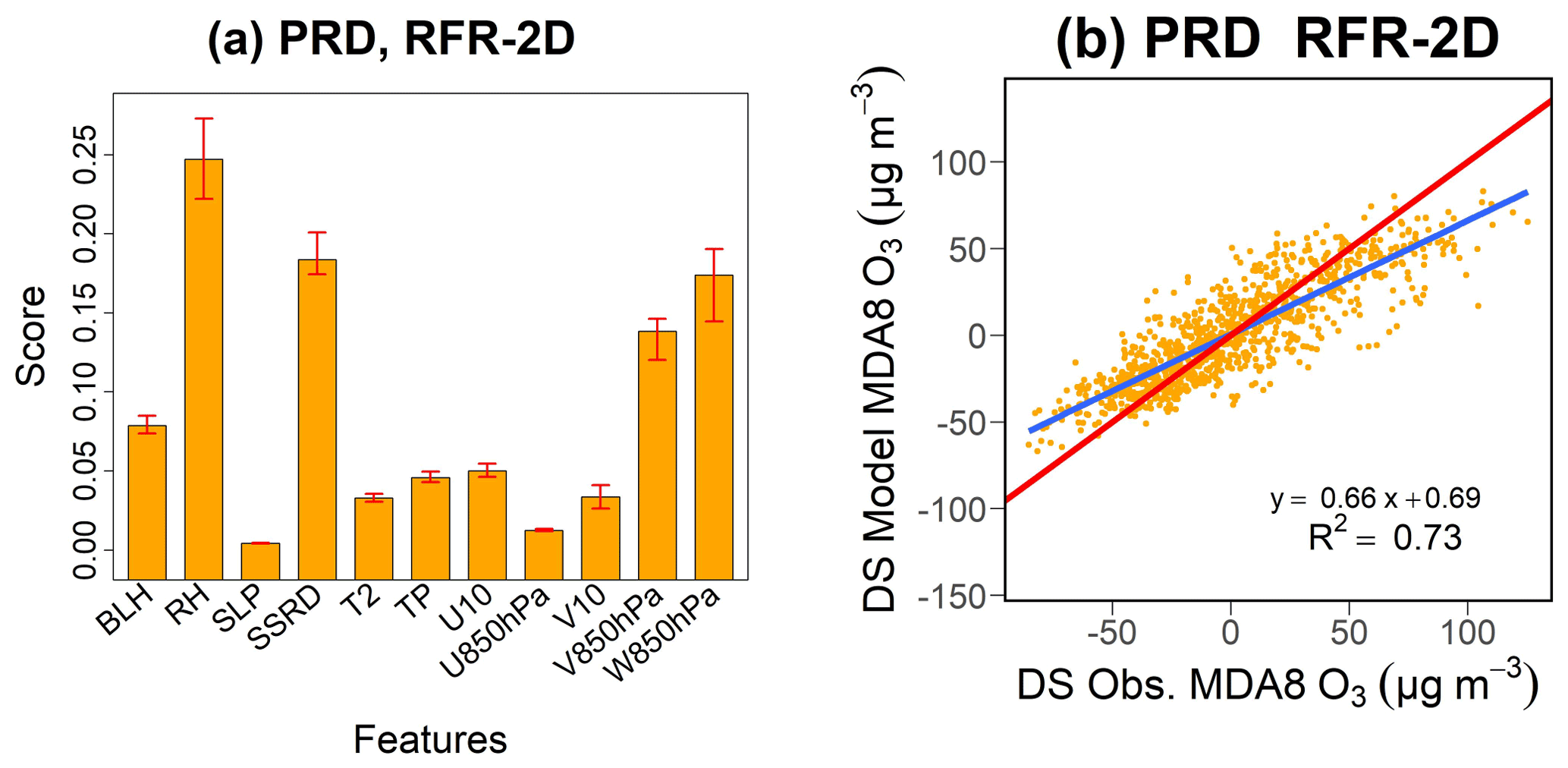
Figure 7(a) Average PRD Gini feature importance score of each meteorological variable if the RFR regressions include non-local predictors within a 7.5∘ longitude × 7.5∘ latitude domain around the predicted grid point; the bar representations are consistent with Fig. 5. (b) Linear fit between RFR–2D predictions and observations in PRD (blue line). The red line equals the ideal 1 : 1 relationship.
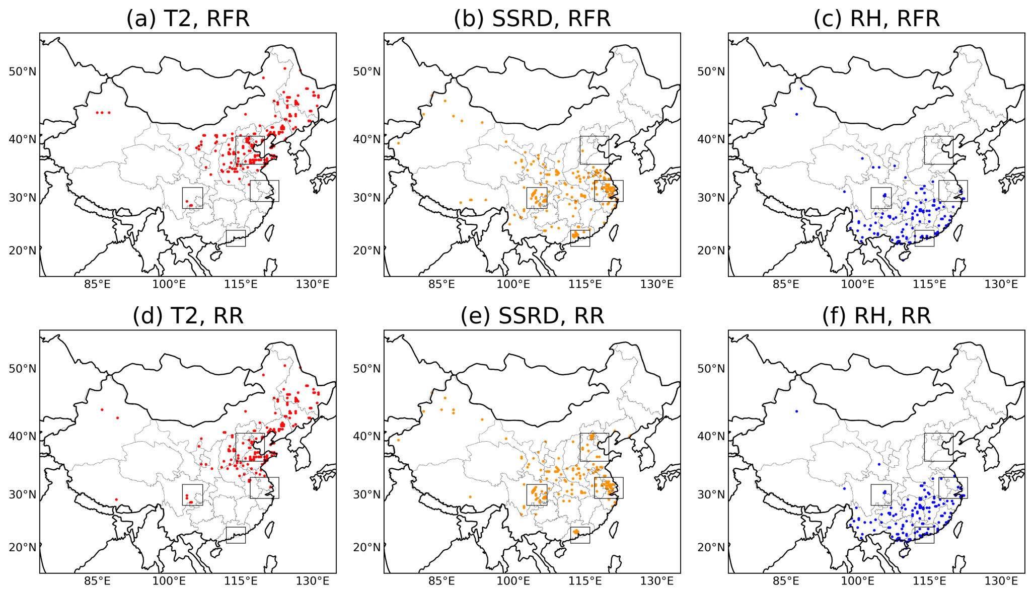
Figure 8(a–c) Most important meteorological driver at each grid location from April–October of 2015–2019 as identified by Gini importance using RFR. (d–f) The same, but using absolute magnitudes for the slopes of RR. Variables as labelled. Relative humidity (RH) dominates in the south and southeast, surface solar radiation downward (SSRD) primarily in central China and eastern China, and temperature at 2 m (T2) in north and northeast China.
A distinct difference in the weather–ozone coupling relationships is found for PRD, where RH is the dominant meteorological driver. Specifically, a negative slope of RH in RR suggests that drier conditions are strongly favourable for peak ozone concentrations in PRD. As one of many possible effects of humidity, ozone may be more destroyed through the photolysis reaction of as O(1D) can subsequently react with H2O, forming OH through reaction of , which will be enhanced in environments with high humidity (Wang et al., 2013; Young et al., 2013). In addition, despite more OH being available given high humidity, OH can react with NO2, forming HNO3 in highly NOx-polluted regions, which ultimately leads to less efficient O3 formation by competing with the oxidation of VOC and CO with OH (Lu et al., 2019a). The negative correlation between humidity and ozone in the PRD region has been identified by previous studies (W. Zhang et al., 2021; Yang et al., 2021; Hua et al., 2008), and the high humidity environment in southern China may be the result of moisture marine air masses transported from tropical region, the South China Sea and western Pacific (W. Zhang et al., 2021; Ding and Chan, 2005). For a nonlinear learning framework using RFR, the second most important meteorological driver in PRD is again the level of surface solar radiation. Interestingly, meridional wind at 850 hPa is key to ozone occurrence in PRD, and it is negatively correlated with average MDA8 ozone. More specifically, the regional average of MDA8 ozone in PRD is negatively correlated with the meridional wind at 850 hPa from the South China Sea (Fig. 6b), indicating strong marine air inflow may have a significant cleaning and dispersion effect on ozone and its precursors in PRD. Furthermore, the negative correlation also expands to the northeast areas of PRD, suggesting lower ozone in PRD given strong southerly wind in these areas, which may hinder the transport of ozone and its precursors to PRD. This finding is consistent with the backward trajectories and numerical modelling analysis by Qu et al. (2021).
Additionally, previous studies (Jiang et al., 2015; Z. Chen et al., 2021; Qu et al., 2021; Wei et al., 2016) also indicate the importance of vertical downward transport of ozone in the southern regions of China due to the impact of typhoons. The effect of such a downward transport may not be well captured by regressions with only local meteorological predictors as it is a larger-scale meteorological phenomenon. Therefore, we refer back to our two-dimensional (2D) approach for RFR in the PRD region first introduced and described in Sect. 3.2. We show the Gini feature importance scores for this 2D domain approach in Fig. 7a. Since we have multiple values of the feature importance for each meteorological variable in this setup (i.e. one for each grid point in the 2D predictor domain), we sum up Gini importance scores for all grid points within the expanded domain for each meteorological variable; and this summed value is denoted as the importance for that particular meteorological variable. As illustrated in Fig. 7a, the relative feature importance of vertical velocity at 850 hPa (W850hPa) increases compared to RFR using only local predictors (see Fig. 5b), likely reflecting the larger-scale influences of downward transport of air masses in the PRD region. Other key meteorological drivers (RH, surface solar radiation and meridional wind at 850 hPa) remain in a similar order to what was identified by purely local regressions. The model performance is slightly improved by adding the 2D information with an increase of R2 to 0.73 (from 0.70) in comparison to the original RFR without 2D expansion. However, we note that the R2 in RFR–2D for PRD region (Fig. 7b) is 0.73 which is slightly less than the R2 using RR–2D (0.76), and the slope of the linear fit between the predictions from RR–2D and the observations is closer to 1 (Fig. 4j) when compared to RFR–2D (Fig. 7b). The higher R2 from RR–2D may be attributed to RR's ability to extrapolate the extreme high/low anomalies of observed ozone, while the prediction range of RFR–2D is more constrained by the range of anomalies from the training data. For example, RR–2D can better predict the extreme low anomaly of observed ozone on 4 October 2015 (Fig. S6). Nevertheless, there could be a trade-off in the feature of extrapolation of RR. For instance, in terms of slope, the seemingly better slope (i.e. closer to 1) from RR–2D (Fig. 4j) may be partly due to its limitation of over- and underpredicting some extreme high/low anomalies, which can be illustrated by outliers from linear fit in Fig. 4j. This can be exemplified by the overprediction of ozone anomaly on 14 April 2015 by RR–2D (also see Fig. S6). Such effects of over- or underpredictions under extrapolation can to a degree compensate for the bias in the predicted versus observed slope, bringing it closer to the 1 : 1 line.
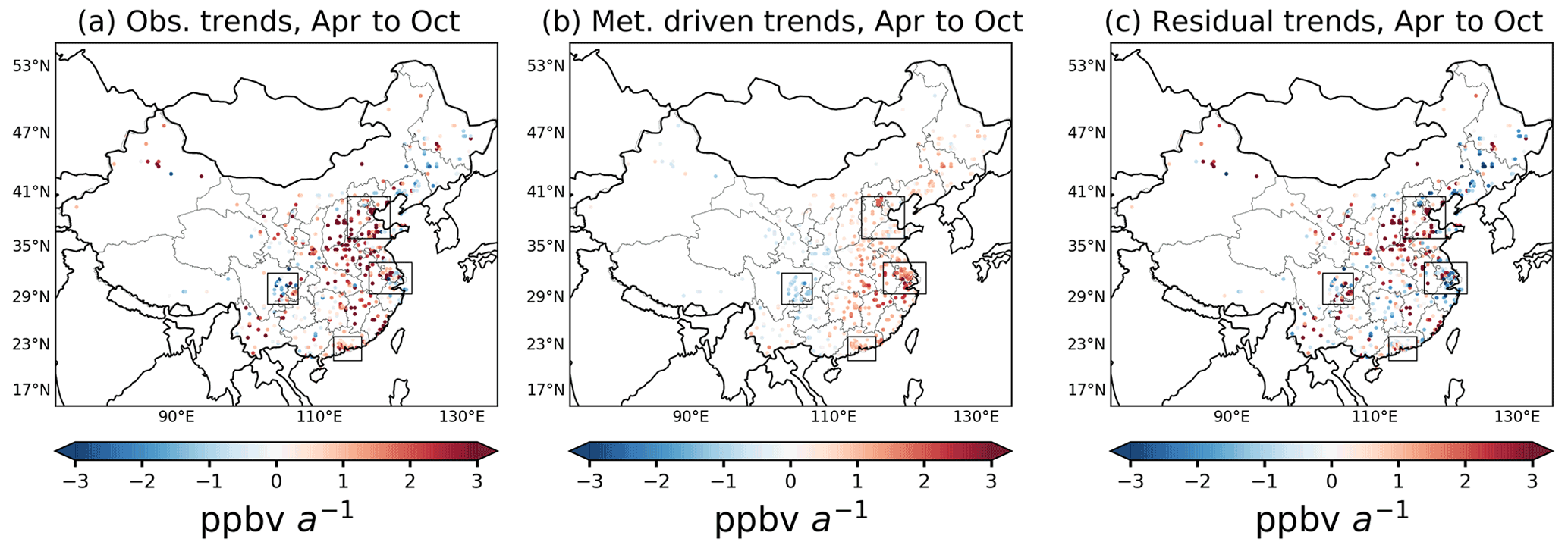
Figure 9Trends of MDA8 ozone during April–October from 2015–2019. Panel (a) shows the observed trends. Panel (b) shows the meteorologically driven trends of MDA8 ozone according to RR–2D. Panel (c) shows the trends of residuals (approximating anthropogenic effects). The trends are estimated by the slopes of ordinary linear regressions fitting each year's April–October MDA8 average ozone values from 2015 to 2019.
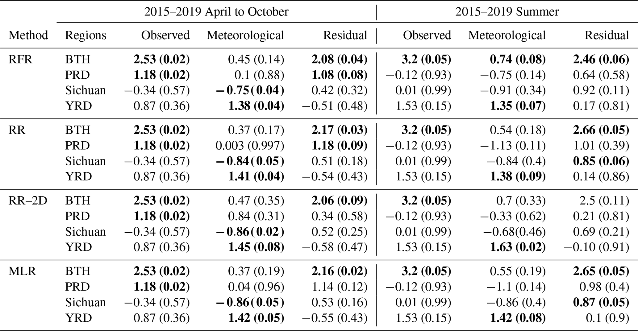
Table 3Observational, meteorological and residual trends of regional averaged MDA8 ozone (ppbv a−1) from 2015–2019 for both April–October and Northern Hemisphere summertime (June, July, August). Values within the brackets are the p values for each trend. Trends and p values are in bold given p values smaller than 0.1.
Across China, we found that there is a consistency in the identification of the three most important meteorological drivers by RFR and RR: temperature, surface solar radiation and RH (Fig. 8). Overall, there is a distinctive distribution pattern of the three major meteorological drivers in China. The temperature at 2 m is dominant over northeast China, covering BTH and expanding to the northern region of China. Most areas in the mid-latitude regions of China, including east China (e.g. YRD) and Sichuan, show surface solar radiation as the main meteorological driver for ozone, suggesting the necessity of including this variable for analyses. The dominance of surface solar radiation gradually expands northward and southward from this region while being overtaken by temperature in the north and RH in the south. Ozone in southern China is primarily driven by RH. Such a distinctive spatial distribution of meteorological drivers may be related to the characteristics of regional climatology. For instance, as described above, regions in southern China such as PRD are particularly influenced by variations in incoming moist air masses, leading to the importance of humidity surpassing temperature and surface solar radiation. The relatively drier northern regions do not have such changeable humidity conditions, making temperature and surface solar radiation the key meteorological factors driving ozone.
3.5 Anthropogenic and meteorological contributions to surface ozone trends from 2015 to 2019
Finally, we explore how our new approach could be used to study the quantitative influence of meteorology on historical ozone variability and trends in China. To facilitate a comparison to previous work, we use a similar method as Li et al. (2020) to establish estimates for observed surface ozone trends in China. We note that our exercise is somewhat limited by the slightly shorter period considered here, i.e. from 2015 to 2019, instead of starting from earlier years. Given this very short period, we are aware that any long-term trend analysis is explorative and has to be interpreted carefully, as will also become evident from low statistical significance in many detected trends. We nevertheless attempt such an analysis to demonstrate how our method can be used in such contexts and to also evaluate if any statistically significant trends are robust after accounting for meteorological influences.
For trend analyses, we first convert MDA8 ozone concentrations from mass concentrations (µg m−3) to volume mixing ratios (ppbv). We then average MDA8 ozone over April to October or summertime for each year for both observational data and model results predicted by our three machine learning-based regressions (RFR, RR and RR–2D) and MLR. Both stepwise MLR and MLR–2D are not included in the trend analyses here since these two algorithms show overall weak performances in modelling ozone (see Table 2). The predictions can be considered as quantitative estimates for the influence of meteorology on the ozone record during the study period. The residual (true ozone signal minus meteorological predictions) will for example be mainly reflective of anthropogenic contributions but will also inevitably contain some uncertainties related to the accuracy of the controlling factor regressions.
Table 3 summarizes the regionally averaged observed trends from 2015 to 2019, which is estimated by ordinary linear regression in the four regions. We additionally list our meteorologically estimated trends and the residual trends. Overall, the three machine learning methods and MLR provide relatively similar estimates of meteorologically driven trends in BTH, YRD and Sichuan, while we find indications that the meteorologically driven trend in PRD may be underestimated by only using local meteorological factors; using RR–2D we estimate a meteorologically driven trend of 0.84 ppbv a−1 during April to October from 2015 to 2019, while RFR, RR and MLR with only local meteorological predictors provide estimates of 0.1, 0.003 and 0.04 ppbv a−1, respectively. Given the better prediction skill in RR–2D for this region (see Table 2 and Fig. 4), this further suggests the importance of spatial meteorological phenomena for ozone trend attribution exercises in the PRD region.
In terms of the raw observed trends, both BTH and PRD show significant increases in ozone pollution (p<0.05) from April to October for 2015 to 2019. We note that the observed trend in PRD is only significant if the months from April to October are considered, whereas there is no significant trend (p=0.93) if only examining months in summertime (JJA). This may be attributed to the ozone's seasonality in PRD where the highest ozone pollution occurs during autumn and the particularly high ozone anomaly during September and October in 2019 (Fig. S7b). We underline that anthropogenic contribution (i.e. the residual) may be overestimated in PRD if only local meteorological factors are considered, given that residuals of RFR, RR and MLR increase compared to RR–2D. For BTH, the positive ozone trend is found to be higher during summertime at 3.20 ppbv a−1 (p=0.05) than if the whole April–October period (2.53 ppbv a−1, p<0.05) is considered. Moreover, estimated by RFR, the meteorologically driven trend in BTH is also higher at 0.74 ppbv a−1 (p<0.1) during summertime than if the whole April–October period is considered (0.45 ppbv a−1; p=0.14). The April–October residual trends in BTH estimated by all four algorithms are all greater than 2 ppbv a−1 (p<0.1), indicating an elevated importance of anthropogenic drivers in BTH. There are no significant observed trends in YRD and Sichuan. However, meteorological factors in both of these regions appear to have a stronger influence on the trends of ozone according to these four algorithms. Additionally, all four methods also agree on meteorologically driven negative trends in Sichuan while positive trends are found for YRD.
Finally, we aim to calculate trends on a ERA5 grid-by-grid point basis. Although both RFR and RR–2D show overall better skill in modelling ozone across China, RR–2D exhibited particularly increased predictive skill in southern China. Therefore, for assessing meteorologically driven trends of MDA8 ozone across all ERA5 grid locations in China, we will only be examining the results for RR–2D. Figure 9 shows trends during April–October from 2015 to 2019 across China. Overall, the observed average trend across China is 1.1 ppbv a−1. The meteorologically driven trend of RR–2D gives the average at 0.5 ppbv a−1 across China, which is around 45 % of the total trend. From Fig. 9a, most regions in eastern China show a positive trend and the magnitudes of increase are more apparent in areas within and nearby BTH, where the ozone pollution increased at an average rate of 2.6 ppbv a−1 across all grids within BTH. We find that the positive trend in those particular regions may be less driven by meteorological factors but indeed might be the result of anthropogenic influences on air pollution (e.g. Liu and Wang, 2020). In YRD, meteorologically driven positive trends are in general the highest in eastern China (average at 1.47 ppbv a−1 across all grids in YRD), which is close to the regionally averaged result by RR–2D (1.45 ppbv a−1, p=0.08) in Table 3. Observed trends in Sichuan are a mixture of both increases and decreases, but meteorologically driven trends are all negative within this region. In PRD, meteorological factors likely played a more central role in driving the recent positive trends in ozone pollution according to our analysis.
Ozone pollution in China can be strongly influenced by meteorological conditions. This study examines the major meteorological drivers for ozone pollution across China during months with particularly high ozone pollution (i.e. April to October, from 2015 to 2019) using a controlling factor framework and two machine learning algorithms, namely RFR and RR.
The results obtained with RFR and RR are also compared with conventional approaches i.e. MLR and stepwise MLR, using consistent out-of-sample cross-validation methods. When considering local meteorological factors only, RFR outperforms the linear approaches RR and MLR, which in turn perform better than stepwise MLR that uses only the three local, most significant meteorological factors. The better performance of RFR is for example evident from the overall increase in predicted versus observed coefficients of determination (R2) ranging from 0.5 to 0.6, as compared to 0.4 to 0.5 for the three linear regressions. Stepwise MLR attains the lowest averaged R2 of all these methods across China. Within the context of using only local meteorological predictors in the regressions, a major advantage of RFR is its ability to model nonlinear relationships between meteorological variables and ozone (e.g. often observed between temperature and ozone). In addition, we tested how the consideration of larger-scale meteorological controlling factors improves our predictive performance. MLR noticeably suffers from the “curse of dimensionality” due to the large increase in the number of predictors when we included additional meteorological information spanning a 7.5∘ × 7.5∘ domain around the target grid point for ozone pollution (the majority of R2 values fall to a lower range of 0.3 to 0.4). In contrast, RR can deal well with this increase in the number of predictors subject to an objective cross-validation approach for its hyperparameter tuning. In particular, despite not directly considering nonlinearity, we find an improvement of model performance in RR with additional two-dimensional predictors, which even outperforms RFR, especially in southern China, indicating the importance of considering a wider meteorological context in future controlling factor analyses of this kind.
A key advantage of our approach is that both RFR and RR allow for a straightforward interpretation of the predictive models (explainable machine learning). Reassuringly, we find a good agreement regarding the identification of the dominant local meteorological drivers for each region. In general, ozone pollution in northern China such as in the BTH region is predominantly driven by temperature fluctuations while ozone in southern China like in the PRD region is particularly strongly controlled by humidity, possibly due to the important role of humid weather in preventing significant ozone pollution episodes in this region. Besides, we observe a strong influence in PRD of air exchange with pristine marine regions, leading to a greater influence of large-scale wind directions, e.g. through the transport of clean marine air into the region, or through air stagnation and ozone accumulation under large-scale sinking atmospheric motion. Surface solar radiation plays a major role in general due to its importance in setting the conditions for ozone photochemistry, which is particularly dominant in YRD and Sichuan. Our work thus highlights that surface solar radiation might be a key predictor to consider in future controlling factor analyses. In summary, hot, dry and sunny weather tends to provide more favourable conditions for ozone pollution in China, which is not entirely unexpected but carries important implications for future changes in air pollution under climate change, while simultaneously considering the pivotal role of targeted emission control strategies on ozone precursors.
In terms of ozone trends, we find a linear MDA8 ozone increase of about 1.1 ppbv a−1 on average during April to October from 2015 to 2019 across China. Regionally, these trends can be more than twice as large as in BTH. The largest positive trends may be mostly attributed to non-meteorological factors such as changes in precursor emissions. However, meteorologically driven trends on average shows increases at 0.5 ppbv a−1 across China, equalling almost 50 % over the period considered here, and it is thus estimated to be a more important factor, especially in southern China and the YRD region. The importance of large-scale meteorological phenomena is highlighted in southern China as a higher averaged meteorological contribution to the increased trend of ozone in PRD and is estimated by RR with nonlocal meteorological predictors. Meteorology appears to have amplified negative ozone trends in the Sichuan region during 2015–2019. However, it is recommended to maintain continuous emission control strategies in this region in order to counter the occurrence of more unfavourable weather conditions for ozone mitigation.
The original air quality data including hourly and 8 h rolling mean of ozone are available at https://quotsoft.net/air/ (last access: 13 July 2021; Wang, 2021). The ERA5 reanalysis product is available at https://cds.climate.copernicus.eu/ (last access: 11 November 2021, Hersbach et al., 2020). Specifically, we use the ERA5 hourly data on pressure levels, available at https://doi.org/10.24381/cds.bd0915c6 (last access: 11 November 2021, Hersbach et al., 2018a) and hourly data on single levels, available at https://doi.org/10.24381/cds.adbb2d47 (last access: 11 November 2021, Hersbach et al., 2018b). The codes for machine learning algorithms are available from the corresponding author upon request.
The supplement related to this article is available online at: https://doi.org/10.5194/acp-22-8385-2022-supplement.
PN, XW and GLF designed the study. XW performed the modelling and analysis of the data, supervised by PN and GLF. XW wrote the paper with input and revision from PN and GLF.
The contact author has declared that neither they nor their co-authors have any competing interests.
Publisher’s note: Copernicus Publications remains neutral with regard to jurisdictional claims in published maps and institutional affiliations.
Peer Nowack was supported through an Imperial College Research Fellowship. We thank the Ministry of Ecology and Environment in China for supporting the nationwide observation network and publishing air quality data. We are grateful to Xiaolei Wang for archiving the air quality data. We thank the European Centre for Medium-Range Weather Forecasts (ECMWF) for providing the ERA5 reanalysis product.
This paper was edited by Qiang Zhang and reviewed by Ke Li and one anonymous referee.
Archibald, A. T., Turnock, S. T., Griffiths, P. T., Cox, T., Derwent, R. G., Knote, C., and Shin, M.: On the changes in surface ozone over the twenty-first century: sensitivity to changes in surface temperature and chemical mechanisms: 21st century changes in surface ozone, Philos. T. R. Soc. A, 378, 20190329, https://doi.org/10.1098/rsta.2019.0329, 2020.
Bishop, C. M.: Pattern recognition and machine learning, Springer Science+Business Media, Singapore, ISBN 978-0387-31073-2, 2006.
Breiman, L.: Random Forests, Mach. Learn., 45, 5–32, https://doi.org/10.1023/A:1010933404324, 2001.
Ceppi, P. and Nowack, P.: Observational evidence that cloud feedback amplifies global warming, P. Natl. Acad. Sci. USA, 118, 1–7, https://doi.org/10.1073/pnas.2026290118, 2021.
Chang, L., Xu, J., Tie, X., and Gao, W.: The impact of Climate Change on the Western Pacific Subtropical High and the related ozone pollution in Shanghai, China, Sci. Rep.-UK, 9, 1–12, https://doi.org/10.1038/s41598-019-53103-7, 2019.
Chen, X., Jiang, Z., Shen, Y., Li, R., Fu, Y., Liu, J., Han, H., Liao, H., Cheng, X., Jones, D. B. A., Worden, H., and Abad, G. G.: Chinese Regulations Are Working – Why Is Surface Ozone Over Industrialized Areas Still High? Applying Lessons From Northeast US Air Quality Evolution, Geophys. Res. Lett., 48, e2021GL092816, https://doi.org/10.1029/2021GL092816, 2021.
Chen, Z., Liu, J., Cheng, X., Yang, M., and Wang, H.: Positive and negative influences of typhoons on tropospheric ozone over southern China, Atmos. Chem. Phys., 21, 16911–16923, https://doi.org/10.5194/acp-21-16911-2021, 2021.
Chinese State Council: Action Plan on Air Pollution Prevention and Control (in Chinese), http://www.gov.cn/zwgk/2013-09/12/content_2486773.htm (last access: 24 November 2021), 2013.
Ding, Y. and Chan, J. C. L.: The East Asian summer monsoon: An overview, Meteorol. Atmos. Phys., 89, 117–142, https://doi.org/10.1007/s00703-005-0125-z, 2005.
Doherty, R. M., Wild, O., Shindell, D. T., Zeng, G., MacKenzie, I. A., Collins, W. J., Fiore, A. M., Stevenson, D. S., Dentener, F. J., Schultz, M. G., Hess, P., Derwent, R. G., and Keating, T. J.: Impacts of climate change on surface ozone and intercontinental ozone pollution: A multi-model study, J. Geophys. Res.-Atmos., 118, 3744–3763, https://doi.org/10.1002/jgrd.50266, 2013.
Dormann, C. F., Elith, J., Bacher, S., Buchmann, C., Carl, G., Carré, G., Marquéz, J. R. G., Gruber, B., Lafourcade, B., Leitão, P. J., Münkemüller, T., Mcclean, C., Osborne, P. E., Reineking, B., Schröder, B., Skidmore, A. K., Zurell, D., and Lautenbach, S.: Collinearity: A review of methods to deal with it and a simulation study evaluating their performance, Ecography, 36, 27–46, https://doi.org/10.1111/j.1600-0587.2012.07348.x, 2013.
Finlayson-Pitts, B. and Pitts, J.: Chemistry of the upper and lower atmosphere: theory, experiments, and applications, Academic Press, San Diego, https://doi.org/10.1016/B978-0-12-257060-5.X5000-X, 2000.
Gao, M., Gao, J., Zhu, B., Kumar, R., Lu, X., Song, S., Zhang, Y., Jia, B., Wang, P., Beig, G., Hu, J., Ying, Q., Zhang, H., Sherman, P., and McElroy, M. B.: Ozone pollution over China and India: seasonality and sources, Atmos. Chem. Phys., 20, 4399–4414, https://doi.org/10.5194/acp-20-4399-2020, 2020.
Grange, S. K., Carslaw, D. C., Lewis, A. C., Boleti, E., and Hueglin, C.: Random forest meteorological normalisation models for Swiss PM10 trend analysis, Atmos. Chem. Phys., 18, 6223–6239, https://doi.org/10.5194/acp-18-6223-2018, 2018.
Gu, Y., Li, K., Xu, J., Liao, H., and Zhou, G.: Observed dependence of surface ozone on increasing temperature in Shanghai, China, Atmos. Environ., 221, 117108, https://doi.org/10.1016/j.atmosenv.2019.117108, 2020.
Guenther, A. B., Zimmerman, P. R., Harley, P. C., Monson, R. K., and Fall, R.: Isoprene and monoterpene emission rate variability: model evaluations and sensitivity analyses, J. Geophys. Res., 98, 12609–12617, https://doi.org/10.1029/93jd00527, 1993.
Han, H., Liu, J., Shu, L., Wang, T., and Yuan, H.: Local and synoptic meteorological influences on daily variability in summertime surface ozone in eastern China, Atmos. Chem. Phys., 20, 203–222, https://doi.org/10.5194/acp-20-203-2020, 2020.
Hersbach, H., Bell, B., Berrisford, P., Biavati, G., Horányi, A., Muñoz Sabater, J., Nicolas, J., Peubey, C., Radu, R., Rozum, I., Schepers, D., Simmons, A., Soci, C., Dee, D., and Thépaut, J.-N.: ERA5 hourly data on pressure levels from 1979 to present, Copernicus Climate Change Service (C3S) Climate Data Store (CDS), [data set], https://doi.org/10.24381/cds.bd0915c6 (last access: 11 November 2021), 2018a.
Hersbach, H., Bell, B., Berrisford, P., Biavati, G., Horányi, A., Muñoz Sabater, J., Nicolas, J., Peubey, C., Radu, R., Rozum, I., Schepers, D., Simmons, A., Soci, C., Dee, D., and Thépaut, J.-N.: ERA5 hourly data on single levels from 1979 to present, Copernicus Climate Change Service (C3S) Climate Data Store (CDS), [data set], https://doi.org/10.24381/cds.adbb2d47 (last access: 11 November 2021), 2018b.
Hersbach, H., Bell, B., Berrisford, P., Hirahara, S., Horányi, A., Muñoz-Sabater, J., Nicolas, J., Peubey, C., Radu, R., Schepers, D., Simmons, A., Soci, C., Abdalla, S., Abellan, X., Balsamo, G., Bechtold, P., Biavati, G., Bidlot, J., Bonavita, M., De Chiara, G., Dahlgren, P., Dee, D., Diamantakis, M., Dragani, R., Flemming, J., Forbes, R., Fuentes, M., Geer, A., Haimberger, L., Healy, S., Hogan, R. J., Hólm, E., Janisková, M., Keeley, S., Laloyaux, P., Lopez, P., Lupu, C., Radnoti, G., de Rosnay, P., Rozum, I., Vamborg, F., Villaume, S., and Thépaut, J. N.: The ERA5 global reanalysis, Q. J. Roy. Meteor. Soc., 146, 1999–2049, https://doi.org/10.1002/qj.3803, 2020.
Hua, W., Chen, Z. M., Jie, C. Y., Kondo, Y., Hofzumahaus, A., Takegawa, N., Chang, C. C., Lu, K. D., Miyazaki, Y., Kita, K., Wang, H. L., Zhang, Y. H., and Hu, M.: Atmospheric hydrogen peroxide and organic hydroperoxides during PRIDE-PRD'06, China: their concentration, formation mechanism and contribution to secondary aerosols, Atmos. Chem. Phys., 8, 6755–6773, https://doi.org/10.5194/acp-8-6755-2008, 2008.
Jacob, D. J.: Heterogeneous chemistry and tropospheric ozone, Atmos. Environ., 34, 2131–2159, https://doi.org/10.1016/S1352-2310(99)00462-8, 2000.
Jiang, Y. C., Zhao, T. L., Liu, J., Xu, X. D., Tan, C. H., Cheng, X. H., Bi, X. Y., Gan, J. B., You, J. F., and Zhao, S. Z.: Why does surface ozone peak before a typhoon landing in southeast China?, Atmos. Chem. Phys., 15, 13331–13338, https://doi.org/10.5194/acp-15-13331-2015, 2015.
Kuhn-Régnier, A., Voulgarakis, A., Nowack, P., Forkel, M., Prentice, I. C., and Harrison, S. P.: The importance of antecedent vegetation and drought conditions as global drivers of burnt area, Biogeosciences, 18, 3861–3879, https://doi.org/10.5194/bg-18-3861-2021, 2021.
Lefohn, A. S., Malley, C. S., Smith, L., Wells, B., Hazucha, M., Simon, H., Naik, V., Mills, G., Schultz, M. G., Paoletti, E., De Marco, A., Xu, X., Zhang, L., Wang, T., Neufeld, H. S., Musselman, R. C., Tarasick, D., Brauer, M., Feng, Z., Tang, H., Kobayashi, K., Sicard, P., Solberg, S., and Gerosa, G.: Tropospheric ozone assessment report: Global ozone metrics for climate change, human health, and crop/ecosystem research, Elementa, 6, 27, https://doi.org/10.1525/elementa.279, 2018.
Lelieveld, J., Evans, J. S., Fnais, M., Giannadaki, D., and Pozzer, A.: The contribution of outdoor air pollution sources to premature mortality on a global scale, Nature, 525, 367–371, https://doi.org/10.1038/nature15371, 2015.
Li, K., Chen, L., Ying, F., White, S. J., Jang, C., Wu, X., Gao, X., Hong, S., Shen, J., Azzi, M., and Cen, K.: Meteorological and chemical impacts on ozone formation: A case study in Hangzhou, China, Atmos. Res., 196, 40–52, https://doi.org/10.1016/j.atmosres.2017.06.003, 2017.
Li, K., Jacob, D. J., Liao, H., Shen, L., Zhang, Q., and Bates, K. H.: Anthropogenic drivers of 2013–2017 trends in summer surface ozone in China, P. Natl. Acad. Sci. USA, 116, 422–427, https://doi.org/10.1073/pnas.1812168116, 2019a.
Li, K., Jacob, D. J., Liao, H., Zhu, J., Shah, V., Shen, L., Bates, K. H., Zhang, Q., and Zhai, S.: A two-pollutant strategy for improving ozone and particulate air quality in China, Nat. Geosci., 12, 906–910, https://doi.org/10.1038/s41561-019-0464-x, 2019b.
Li, K., Jacob, D. J., Shen, L., Lu, X., De Smedt, I., and Liao, H.: Increases in surface ozone pollution in China from 2013 to 2019: Anthropogenic and meteorological influences, Atmos. Chem. Phys., 20, 11423–11433, https://doi.org/10.5194/acp-20-11423-2020, 2020.
Liu, Y. and Wang, T.: Worsening urban ozone pollution in China from 2013 to 2017 – Part 2: The effects of emission changes and implications for multi-pollutant control, Atmos. Chem. Phys., 20, 6323–6337, https://doi.org/10.5194/acp-20-6323-2020, 2020.
Lu, X., Zhang, L., and Shen, L.: Meteorology and Climate Influences on Tropospheric Ozone: a Review of Natural Sources, Chemistry, and Transport Patterns, Curr. Pollut. Reports, 5, 238–260, https://doi.org/10.1007/s40726-019-00118-3, 2019a.
Lu, X., Zhang, L., Chen, Y., Zhou, M., Zheng, B., Li, K., Liu, Y., Lin, J., Fu, T.-M., and Zhang, Q.: Exploring 2016–2017 surface ozone pollution over China: source contributions and meteorological influences, Atmos. Chem. Phys., 19, 8339–8361, https://doi.org/10.5194/acp-19-8339-2019, 2019b.
Ma, M., Gao, Y., Wang, Y., Zhang, S., Leung, L. R., Liu, C., Wang, S., Zhao, B., Chang, X., Su, H., Zhang, T., Sheng, L., Yao, X., and Gao, H.: Substantial ozone enhancement over the North China Plain from increased biogenic emissions due to heat waves and land cover in summer 2017, Atmos. Chem. Phys., 19, 12195–12207, https://doi.org/10.5194/acp-19-12195-2019, 2019.
Mansfield, L. A., Nowack, P. J., Kasoar, M., Everitt, R. G., Collins, W. J., and Voulgarakis, A.: Predicting global patterns of long-term climate change from short-term simulations using machine learning, npj Clim. Atmos. Sci., 3, 44, https://doi.org/10.1038/s41612-020-00148-5, 2020.
McDonald, G. C.: Ridge regression, WIREs Comput. Stat., 1, 93–100, https://doi.org/10.1002/wics.14, 2009.
Meehl, G. A., Tebaldi, C., Tilmes, S., Lamarque, J. F., Bates, S., Pendergrass, A., and Lombardozzi, D.: Future heat waves and surface ozone, Environ. Res. Lett., 13, 064004, https://doi.org/10.1088/1748-9326/aabcdc, 2018.
Menze, B. H., Kelm, B. M., Masuch, R., Himmelreich, U., Bachert, P., Petrich, W., and Hamprecht, F. A.: A comparison of random forest and its Gini importance with standard chemometric methods for the feature selection and classification of spectral data, BMC Bioinformatics, 10, 1–16, https://doi.org/10.1186/1471-2105-10-213, 2009.
MEP: Technical regulation for ambient air quality assessment (on trial) (HJ 663-2013) (in Chinese), https://www.mee.gov.cn/ywgz/fgbz/bz/bzwb/jcffbz/201309/t20130925_260809.shtml (last access: 24 November 2021), 2013.
Monks, P. S., Archibald, A. T., Colette, A., Cooper, O., Coyle, M., Derwent, R., Fowler, D., Granier, C., Law, K. S., Mills, G. E., Stevenson, D. S., Tarasova, O., Thouret, V., Von Schneidemesser, E., Sommariva, R., Wild, O., and Williams, M. L.: Tropospheric ozone and its precursors from the urban to the global scale from air quality to short-lived climate forcer, Atmos. Chem. Phys., 15, 8889–8973, https://doi.org/10.5194/acp-15-8889-2015, 2015.
Ning, G., Yim, S. H. L., Yang, Y., Gu, Y., and Dong, G.: Modulations of synoptic and climatic changes on ozone pollution and its health risks in mountain-basin areas, Atmos. Environ., 240, 117808, https://doi.org/10.1016/j.atmosenv.2020.117808, 2020.
Nowack, P., Braesicke, P., Haigh, J., Abraham, N. L., Pyle, J., and Voulgarakis, A.: Using machine learning to build temperature-based ozone parameterizations for climate sensitivity simulations, Environ. Res. Lett., 13, 104016, https://doi.org/10.1088/1748-9326/aae2be, 2018.
Nowack, P., Konstantinovskiy, L., Gardiner, H., and Cant, J.: Machine learning calibration of low-cost NO2 and PM10 sensors: non-linear algorithms and their impact on site transferability, Atmos. Meas. Tech., 14, 5637–5655, https://doi.org/10.5194/amt-14-5637-2021, 2021.
Otero, N., Sillmann, J., Mar, K. A., Rust, H. W., Solberg, S., Andersson, C., Engardt, M., Bergström, R., Bessagnet, B., Colette, A., Couvidat, F., Cuvelier, C., Tsyro, S., Fagerli, H., Schaap, M., Manders, A., Mircea, M., Briganti, G., Cappelletti, A., Adani, M., D'Isidoro, M., Pay, M.-T., Theobald, M., Vivanco, M. G., Wind, P., Ojha, N., Raffort, V., and Butler, T.: A multi-model comparison of meteorological drivers of surface ozone over Europe, Atmos. Chem. Phys., 18, 12269–12288, https://doi.org/10.5194/acp-18-12269-2018, 2018.
Ou, J., Yuan, Z., Zheng, J., Huang, Z., Shao, M., Li, Z., Huang, X., Guo, H., and Louie, P. K. K.: Ambient Ozone Control in a Photochemically Active Region: Short-Term Despiking or Long-Term Attainment?, Environ. Sci. Technol., 50, 5720–5728, https://doi.org/10.1021/acs.est.6b00345, 2016.
Pu, X., Wang, T. J., Huang, X., Melas, D., Zanis, P., Papanastasiou, D. K., and Poupkou, A.: Enhanced surface ozone during the heat wave of 2013 in Yangtze River Delta region, China, Sci. Total Environ., 603–604, 807–816, https://doi.org/10.1016/j.scitotenv.2017.03.056, 2017.
Qi, J., Zheng, B., Li, M., Yu, F., Chen, C., Liu, F., Zhou, X., Yuan, J., Zhang, Q., and He, K.: A high-resolution air pollutants emission inventory in 2013 for the Beijing-Tianjin-Hebei region, China, Atmos. Environ., 170, 156–168, https://doi.org/10.1016/j.atmosenv.2017.09.039, 2017.
Qu, K., Wang, X., Yan, Y., Shen, J., Xiao, T., Dong, H., Zeng, L., and Zhang, Y.: A comparative study to reveal the influence of typhoons on the transport, production and accumulation of O3 in the Pearl River Delta, China, Atmos. Chem. Phys., 21, 11593–11612, https://doi.org/10.5194/acp-21-11593-2021, 2021.
Scikit-learn: sklearn.metrics.r2_score, https://scikit-learn.org/stable/modules/generated/sklearn.metrics.r2_score.html, last access: 13 April 2022.
Shu, L., Xie, M., Wang, T., Gao, D., Chen, P., Han, Y., Li, S., Zhuang, B., and Li, M.: Integrated studies of a regional ozone pollution synthetically affected by subtropical high and typhoon system in the Yangtze River Delta region, China, Atmos. Chem. Phys., 16, 15801–15819, https://doi.org/10.5194/acp-16-15801-2016, 2016.
Shu, L., Wang, T., Han, H., Xie, M., Chen, P., Li, M., and Wu, H.: Summertime ozone pollution in the Yangtze River Delta of eastern China during 2013–2017: Synoptic impacts and source apportionment, Environ. Pollut., 257, 113631, https://doi.org/10.1016/j.envpol.2019.113631, 2020.
Sillman, S.: The relation between ozone, NOx and hydrocarbons in urban and polluted rural environments, Atmos. Environ., https://doi.org/10.1016/S1352-2310(98)00345-8, 1999.
Song, C., Liu, B., Dai, Q., Li, H., and Mao, H.: Temperature dependence and source apportionment of volatile organic compounds (VOCs) at an urban site on the north China plain, Atmos. Environ., 207, 167–181, https://doi.org/10.1016/j.atmosenv.2019.03.030, 2019.
Squire, O. J., Archibald, A. T., Griffiths, P. T., Jenkin, M. E., Smith, D., and Pyle, J. A.: Influence of isoprene chemical mechanism on modelled changes in tropospheric ozone due to climate and land use over the 21st century, Atmos. Chem. Phys., 15, 5123–5143, https://doi.org/10.5194/acp-15-5123-2015, 2015.
Stirnberg, R., Cermak, J., Kotthaus, S., Haeffelin, M., Andersen, H., Fuchs, J., Kim, M., Petit, J.-E., and Favez, O.: Meteorology-driven variability of air pollution (PM1) revealed with explainable machine learning, Atmos. Chem. Phys., 21, 3919–3948, https://doi.org/10.5194/acp-21-3919-2021, 2021.
Tan, Z., Hofzumahaus, A., Lu, K., Brown, S. S., Holland, F., Huey, L. G., Kiendler-Scharr, A., Li, X., Liu, X., Ma, N., Min, K. E., Rohrer, F., Shao, M., Wahner, A., Wang, Y., Wiedensohler, A., Wu, Y., Wu, Z., Zeng, L., Zhang, Y., and Fuchs, H.: No Evidence for a Significant Impact of Heterogeneous Chemistry on Radical Concentrations in the North China Plain in Summer 2014, Environ. Sci. Technol., 54, 5973–5979, https://doi.org/10.1021/acs.est.0c00525, 2020.
Wang, H., Wu, K., Liu, Y., Sheng, B., Lu, X., He, Y., Xie, J., Wang, H., and Fan, S.: Role of Heat Wave-Induced Biogenic VOC Enhancements in Persistent Ozone Episodes Formation in Pearl River Delta, J. Geophys. Res.-Atmos., 126, e2020JD034317, https://doi.org/10.1029/2020JD034317, 2021.
Wang, N., Lyu, X., Deng, X., Huang, X., Jiang, F., and Ding, A.: Aggravating O3 pollution due to NOx emission control in eastern China, Sci. Total Environ., 677, 732–744, https://doi.org/10.1016/j.scitotenv.2019.04.388, 2019.
Wang, T., Xue, L., Brimblecombe, P., Lam, Y. F., Li, L., and Zhang, L.: Ozone pollution in China: A review of concentrations, meteorological influences, chemical precursors, and effects, Sci. Total Environ., 575, 1582–1596, https://doi.org/10.1016/j.scitotenv.2016.10.081, 2017.
Wang, X. L.: Historical air quality data in China, https://quotsoft.net/air/, last access: 13 July 2021.
Wang, Y., Shen, L., Wu, S., Mickley, L., He, J., and Hao, J.: Sensitivity of surface ozone over China to 2000–2050 global changes of climate and emissions, Atmos. Environ., 75, 374–382, https://doi.org/10.1016/j.atmosenv.2013.04.045, 2013.
Wei, X., Lam, K. S., Cao, C., Li, H., and He, J.: Dynamics of the Typhoon Haitang Related High Ozone Episode over Hong Kong, Adv. Meteorol., 2016, 6089154, https://doi.org/10.1155/2016/6089154, 2016.
Xie, X., Shao, M., Liu, Y., Lu, S., Chang, C. C., and Chen, Z. M.: Estimate of initial isoprene contribution to ozone formation potential in Beijing, China, Atmos. Environ., 42, 6000–6010, https://doi.org/10.1016/j.atmosenv.2008.03.035, 2008.
Yang, L., Xie, D., Yuan, Z., Huang, Z., Wu, H., Han, J., Liu, L., and Jia, W.: Quantification of regional ozone pollution characteristics and its temporal evolution: Insights from identification of the impacts of meteorological conditions and emissions, Atmosphere, 12, 279, https://doi.org/10.3390/atmos12020279, 2021.
Young, P. J., Archibald, A. T., Bowman, K. W., Lamarque, J.-F., Naik, V., Stevenson, D. S., Tilmes, S., Voulgarakis, A., Wild, O., Bergmann, D., Cameron-Smith, P., Cionni, I., Collins, W. J., Dalsøren, S. B., Doherty, R. M., Eyring, V., Faluvegi, G., Horowitz, L. W., Josse, B., Lee, Y. H., MacKenzie, I. A., Nagashima, T., Plummer, D. A., Righi, M., Rumbold, S. T., Skeie, R. B., Shindell, D. T., Strode, S. A., Sudo, K., Szopa, S., and Zeng, G.: Pre-industrial to end 21st century projections of tropospheric ozone from the Atmospheric Chemistry and Climate Model Intercomparison Project (ACCMIP), Atmos. Chem. Phys., 13, 2063–2090, https://doi.org/10.5194/acp-13-2063-2013, 2013.
Zhai, S., Jacob, D. J., Wang, X., Shen, L., Li, K., Zhang, Y., Gui, K., Zhao, T., and Liao, H.: Fine particulate matter (PM2.5) trends in China, 2013–2018: separating contributions from anthropogenic emissions and meteorology, Atmos. Chem. Phys., 19, 11031–11041, https://doi.org/10.5194/acp-19-11031-2019, 2019.
Zhang, J., Gao, Y., Luo, K., Leung, L. R., Zhang, Y., Wang, K., and Fan, J.: Impacts of compound extreme weather events on ozone in the present and future, Atmos. Chem. Phys., 18, 9861–9877, https://doi.org/10.5194/acp-18-9861-2018, 2018.
Zhang, W., Zou, Y., Zheng, X. D., Wang, N., Yan, H., Chen, Y. P., Zhao, X. J., Ji, Z. P., Li, F., Mai, B. R., Yin, C. Q., Deng, T., Fan, L. Y., and Deng, X. J.: Characteristics of the vertical distribution of tropospheric ozone in late autumn at Yangjiang station in Pearl River Delta (PRD), China. Part I: Observed event, Atmos. Environ., 244, 117898, https://doi.org/10.1016/j.atmosenv.2020.117898, 2021.
Zhang, X., Fung, J. C. H., Lau, A. K. H., Hossain, M. S., Louie, P. K. K., and Huang, W.: Air quality and synergistic health effects of ozone and nitrogen oxides in response to China's integrated air quality control policies during 2015–2019, Chemosphere, 268, 129385, https://doi.org/10.1016/j.chemosphere.2020.129385, 2021.
Zhao, X., Yu, B., Liu, Y., Chen, Z., Li, Q., Wang, C., and Wu, J.: Estimation of poverty using random forest regression with multi-source data: A case study in Bangladesh, Remote Sens., 11, 1–18, https://doi.org/10.3390/rs11040375, 2019.
Zheng, B., Tong, D., Li, M., Liu, F., Hong, C., Geng, G., Li, H., Li, X., Peng, L., Qi, J., Yan, L., Zhang, Y., Zhao, H., Zheng, Y., He, K., and Zhang, Q.: Trends in China's anthropogenic emissions since 2010 as the consequence of clean air actions, Atmos. Chem. Phys., 18, 14095–14111, https://doi.org/10.5194/acp-18-14095-2018, 2018.