the Creative Commons Attribution 4.0 License.
the Creative Commons Attribution 4.0 License.
 | 18 Jan 2022
Box model trajectory studies of contrail formation using a particle-based cloud microphysics scheme
Andreas Bier
Simon Unterstrasser
Xavier Vancassel
We investigate the microphysics of contrail formation behind commercial aircraft by means of the particle-based LCM (Lagrangian Cloud Module) box model. We extend the original LCM to cover the basic pathway of contrail formation on soot particles being activated into liquid droplets that soon after freeze into ice crystals. In our particle-based microphysical approach, simulation particles are used to represent different particle types (soot, droplets, ice crystals) and properties (mass/radius, number). The box model is applied in two frameworks. In the classical framework, we prescribe the dilution along one average trajectory in a single box model run. In the second framework, we perform a large ensemble of box model runs using 25 000 different trajectories inside an expanding exhaust jet as simulated by the LES (large-eddy simulation) model FLUDILES.
In the ensemble runs, we see a strong radial dependence of the temperature and relative humidity evolution. Droplet formation on soot particles happens first near the plume edge and a few tenths of a second later in the plume centre. Averaging over the ensemble runs, the number of formed droplets and ice crystals increases more smoothly over time than for the single box model run with the average dilution.
Consistent with previous studies, contrail ice crystal number varies strongly with atmospheric parameters like temperature and relative humidity near the contrail formation threshold. Close to this threshold, the apparent ice number emission index (product of freezing fraction and soot number emission index) strongly depends on the geometric-mean dry core radius and the hygroscopicity parameter of soot particles. The freezing fraction of soot particles slightly decreases with increasing soot particle number, particularly for higher soot number emissions. This weakens the increase of the apparent ice number emission index with rising soot number emission index.
Comparison with box model results of a recent contrail formation study by Lewellen (2020) (using similar microphysics) shows a later onset of our contrail formation due to a weaker prescribed plume dilution. If we use the same dilution data, our evolution and Lewellen's evolution in contrail ice nucleation show an excellent agreement cross-verifying both microphysics implementations. This means that differences in contrail properties mainly result from different representations of the plume mixing and not from the microphysical modelling.
Using an ensemble mean framework instead of a single trajectory does not necessarily lead to an improved scientific outcome. Contrail ice crystal numbers tend to be overestimated since the interaction between the different trajectories is not considered.
The presented aerosol and microphysics scheme describing contrail formation is of intermediate complexity and thus suited to be incorporated in an LES model for 3D contrail formation studies explicitly simulating the jet expansion. Our box model results will help interpret the upcoming, more complex 3D results.
- Article
(3554 KB) - Full-text XML
-
Supplement
(692 KB) - BibTeX
- EndNote


Aviation contributes to around 5 % of the anthropogenic climate impact (Lee et al., 2021), where contrail cirrus is the largest known contributor in terms of radiative forcing (e.g. Boucher et al., 2013; Bock and Burkhardt, 2016). Due to projections of large increases in air traffic, this contribution is expected to increase significantly (Bock and Burkhardt, 2019). The number of nucleated contrail ice crystals has a large impact on contrail cirrus properties and their life cycle (e.g. Unterstrasser and Gierens, 2010; Bier et al., 2017; Burkhardt et al., 2018). The formation of contrails depends on complex (thermo)dynamic, microphysical and chemical processes in the exhaust plume, leading to a large variability in initial ice crystal numbers.
Measurements and observations implicate that contrails form once the plume mixture between the exhaust and ambient air reaches or surpasses water saturation. This condition is mathematically cast in form of the Schmidt–Appleman (SA) criterion, a relation derived purely from the thermodynamics of the mixing process (Schumann, 1996).
Plume exhaust particles, in particular soot but also ambient particles entrained into the plume, can activate into water droplets and subsequently freeze to ice crystals by homogeneous nucleation (Kärcher et al., 2015). Ultrafine volatile particles resulting from recombination of ion clusters and molecules (Yu and Turco, 1997) may also contribute to the formation of ice crystals but typically require high (> 10 %) water supersaturation to form water droplets due to their small size of a few nanometres (Kärcher and Yu, 2009). Contrail ice nucleation typically occurs within the first second of plume mixing during the jet phase.
Several studies on contrail formation in jet exhaust plumes have been conducted in the past. At the moment, there are basically two complementary model approaches to study the contrail formation which either focus on jet dynamics or on plume microphysics. On the one hand, 0D box models based on a few idealized air parcel trajectories originating from an engine (e.g. Kärcher and Yu, 2009; Wong and Miake-Lye, 2010) are in general equipped with detailed microphysical and chemical schemes. However, they neglect the large spatial variability in jet plumes arising from turbulent mixing of the hot exhaust with ambient air and simulate only an average mixing state over the whole plume cross-sectional area. Spatial inhomogeneities (in particular, strong radial gradients and turbulent perturbations) in plume temperature and relative humidity are not considered. This leads to uncertainties in representing contrail ice crystal formation with unclear implications on contrail properties during the subsequent vortex and dispersion phase. On the other hand, several three-dimensional (3D) large-eddy simulations (LESs) studying the contrail formation in the near-field plume (Paoli et al., 2013; Khou et al., 2015, 2017) resolve many details of the jet flow and account for spatial variation in the plume. Even though they are equipped with sophisticated aerosol and chemical models, they have a simplified representation of microphysical processes. The main assumption in those 3D studies is that contrail formation is triggered by heterogeneous ice nucleation on chemically activated soot particles following Kärcher (1998). Chemical activation means that at least 10 % of the particle surface needs to be covered with sulfuric acid to form a thin liquid layer around the particle due to adsorption of water molecules. First, these studies assume plume water saturation to be sufficient for the activation of soot particles, but the Kelvin effect requires, in particular for soot particles with sizes of a few nanometres, that water saturation is clearly surpassed. This might cause a significant overestimation of the number of formed ice crystals. Second, experimental investigations have shown that fresh engine soot particles are not supposed to be good ice nuclei (e.g. Bond et al., 2013). This strengthens the requirement of a transient liquid phase according to the SA criterion. Third, aviation soot develops through incomplete combustion of hydrocarbons (Bockhorn, 1994) and is mainly composed of elementary carbon, causing a weak hygroscopicity. Laboratory studies reveal the existence of active sites on soot particles, which develop by the attachment of functional groups and enable the adsorption of water molecules (Popovicheva et al., 2017). Since nitrate species and hydroxyls also have a great potential to interact with soot particles (e.g. Kärcher et al., 1996; Grimonprez et al., 2018), the coating of soot by sulfuric acid is not mandatory for their activation into water droplets. This fact explains why visible contrails can still form when almost desulfurized fuel is burnt (Busen and Schumann, 1995).
Lewellen (2020) uses the more appropriate microphysical pathway consistent with the SA criterion and considers soot, ambient and volatile particles as exhaust particle types potentially activating into water droplets and forming ice crystals. However, these exhaust particles are assumed to have a monodisperse (or at best bidisperse) size distribution. This does not sufficiently capture the Kelvin effect-related competition among differently sized aerosol particles and possibly leads to ice crystal size spectra that are too narrow. In general, Lewellen (2020) investigated the sensitivity of contrail ice crystal numbers to properties of the different exhaust particles and to ambient conditions as well as engine configurations, both within 3D LES and within a box model. Many findings related to contrail formation rely on results from box models or analytical approaches with a crude representation of plume heterogeneity. By employing the same microphysics in 3D LES and in a box model with a mean dilution derived from the former model, Lewellen (2020) highlights for which parameter configurations findings drawn from box model results are similar to those from 3D LES. Contrail ice crystal numbers per burnt fuel mass are consistent in both model frameworks for low exhaust particle numbers or in scenarios where ice crystals mainly form on ambient aerosol particles. However, the box model generally overestimates these ice crystal numbers for soot particle numbers of current engines/fuels. Moreover, the ice crystal formation on emitted ultrafine volatile particles becomes more substantial in the LES than in the box model.
The basic objective of the project “ConForm” funded by the Deutsche Forschungsgemeinschaft (DFG) is to combine the advantages of the two complementary approaches, which means to simulate contrail formation in the expanding jet by means of 3D LES with an improved representation of cloud microphysics. For this, we will employ the LES model EULAG (Smolarkiewicz and Grell, 1992), which is fully coupled with the particle-based ice microphysics scheme LCM (Lagrangian Cloud Module; Sölch and Kärcher, 2010). The model system EULAG-LCM has been used for contrail simulations during the vortex phase (e.g. Unterstrasser, 2014) and the dispersion phase (e.g. Unterstrasser et al., 2017a, b). This has been done with an EULAG version that does not yet support the compressible and gas dynamics equations. Hence in a next step, LCM will be coupled to an up-to-date EULAG version that accounts for compressibility effects in the jet plume.
So far, LCM includes ice crystal formation as it occurs in natural cirrus clouds. The present paper describes how the LCM model has been extended in order to cover the specifics of contrail formation and is a first step towards the goals of ConForm. Our main objective is to test the extended LCM in a simple dynamical framework by running it in a box model set-up. The microphysical parameterization is similar to that in Lewellen (2020), but the numerical approach of the microphysics differs as our study relies on a particle-based description and not on an Eulerian spectral bin model. Moreover, we prescribe soot particles by a log-normal instead of a monodisperse or bidisperse size distribution.
Paoli et al. (2008) and Vancassel et al. (2014) extended the box model framework to a multi-0D approach. Here, “multi-0D” means that the box model was run for a large ensemble of trajectories that sample the expanding jet plume as provided by 3D LES and that represent many different plume dilution developments. In such an “offline” approach, the microphysics can be more advanced than in a full 3D framework with “online” microphysics. In our study, we intend to highlight the importance of the huge variability in thermodynamic and contrail properties resulting from the variability in the inhomogeneous turbulent mixed jet plume. Therefore, we will use an ensemble of many trajectories where the data have been taken from Vancassel et al. (2014). We expect that the temporal evolution of ensemble mean properties leads to improved scientific results compared to those using one single average trajectory.
Paoli et al. (2008) mainly studied the temporal evolution of concentrations and (apparent) emission indices of volatile particles and ice crystals depending on the fuel sulfur content. Vancassel et al. (2014) revealed the spatial variability in thermodynamic quantities and contrail properties. Moreover, they used an online method with less detailed contrail microphysics and an offline method with more detailed contrail microphysics and highlighted differences between the methods. The two studies have the following improvements compared to the online 3D studies of Khou et al. (2015, 2017): they include different types of aerosol particles, the chemical processing of fuel sulfur and the formation and growth of volatile particles. Curvature and the solution effect are accounted for. A further improvement is prescribing log-normally size-distributed soot particles using 60 size bins and varying the geometric-mean dry core radius between 10 and 30 nm.
For conventional aircraft engines, soot particles are in general the major source for the formation of contrail ice crystals (e.g. Kärcher et al., 1996; Kärcher and Yu, 2009; Kleine et al., 2018). The number of emitted soot particles significantly influences the contrail cirrus climate impact (Burkhardt et al., 2018). Since engine soot emissions are quite variable and uncertain, particularly in terms of their number and size (e.g. Anderson et al., 1998; Petzold et al., 1999; Schumann et al., 2002; Agarwal et al., 2019), our main focus is to investigate the sensitivity of contrail properties (during their formation stage) to different specific soot properties. We will also analyse the variability of contrail ice nucleation with ambient conditions as already explored by Bier and Burkhardt (2019) using the analytical parameterization of Kärcher et al. (2015).
This section gives a short overview of the basic Lagrangian Cloud Module (LCM) (Sect. 2.1), which has been extensively used for simulations of natural cirrus as well as young and aged contrails in the recent past. Section 2.2 then describes in more detail the modifications and extensions for simulating contrail formation, and Sect. 2.3 gives an overview about the general plume evolution and our trajectory data. Finally, we will explain the box model framework in which LCM is employed in the present study.
2.1 Particle-based LCM microphysics
The particle-based ice microphysics model LCM (Sölch and Kärcher, 2010) comprises explicit aerosol and ice microphysics and is employed for the simulation of pure ice clouds like natural cirrus (e.g. Sölch and Kärcher, 2011) or contrails (e.g. Unterstrasser, 2014; Unterstrasser and Görsch, 2014; Unterstrasser et al., 2017a, b). In a particle-based microphysical approach, hydrometeors (like ice crystals or water droplets) are described by simulation particles (SIPs) unlike traditional Eulerian approaches, where cloud properties are usually described by field variables. LCM has been used in conjunction with the LES flow solver EULAG, which computes the evolution of momentum, temperature and water vapour. We omit the details about the coupling between EULAG and LCM as in the present box model approach background temperature and water vapour concentration are prescribed and not simulated. Each SIP represents a certain number νi of real ice crystals with identical properties and stores information about the single ice crystal mass mi, the weighting factor νi and the ice crystal habit, among others. Microphysical processes on the simulation particles include homogeneous freezing of liquid super-cooled aerosol particles, heterogeneous ice nucleation, deposition growth of ice crystals, sedimentation, aggregation, latent heat release and radiative impact on particle growth. For the contrail formation simulations, many of those processes (e.g. aggregation, sedimentation, radiation-related effects) are switched off. In the extended LCM, which will be described next, initial SIPs represent soot particles, which then become activated into water droplets and eventually freeze (assuming suitable background conditions). The SIP data structure is augmented and stores information about the particle type (soot, droplet, ice crystal) and properties (number, mass/radius, freezing temperature).
2.2 Microphysics of contrail formation
2.2.1 Exhaust particles
In this study, we consider soot to be the only exhaust particle since it plays a major role for contrail formation behind conventional passenger aircraft (e.g. Kärcher et al., 1996; Kärcher and Yu, 2009; Kleine et al., 2018). Background particles will become relevant for aircraft with soot-poor or even soot-free emissions as for liquid hydrogen propulsion (Kärcher et al., 2015; Rojo et al., 2015). Even though ultrafine volatile particles become more substantial for contrail ice crystal formation in a 3D LES set-up (Lewellen, 2020), they are supposed to have a tiny impact on contrail formation for current soot-rich emissions in a box model framework (Kärcher and Yu, 2009). Hence, we neglect volatile particles in the present study, but we will incorporate this particle type in the next model version.
The size spectrum of soot particles ranges from a few to hundreds of nanometres with geometric-mean values of around 15 nm (Petzold et al., 1999). Soot particles are composed of several nanometre-sized primary spherules combined into aggregates. For simplicity, we assume a spherical shape. Recent studies indicate a fractal irregular shape of the larger (more than several 10 nm) soot particles (e.g. Wang et al., 2019; Distaso et al., 2020). Taking this into account would modify their effective surface area and, therefore, the activation into water droplets and condensational growth rates. But it would require additional complexity that may not be relevant in such an intermediate detailed microphysical approach.
We prescribe log-normally size distributed soot particles by an ensemble of NSIP simulation particles (SIPs) using a technique described in Appendix A of Unterstrasser and Sölch (2014). In a priori tests, we performed simulations with different values of NSIP ranging from 50 to 200. We find converged results of the analysed contrail properties for NSIP above around 100. Since this threshold value slightly varies with the geometric-mean dry core radius and particle size distribution width, we choose a default value of around NSIP=130.
2.2.2 Basic formation pathway
In general, the moist exhaust plume cools due to mixing with ambient air. Contrails can form if ambient temperature is below the so-called Schmidt–Appleman (SA) threshold temperature (ΘG), and the plume becomes water-supersaturated in a certain temperature range. The threshold temperature varies with atmospheric parameters (ambient relative humidity over water, air pressure) and engine/fuel properties (specific combustion heat, propulsion efficiency, water vapour emission index). The calculation of ΘG is described in Appendix 2 of Schumann (1996).
We use the Kappa–Köhler theory (Sect. 2.2.3) to calculate which soot particles are able to activate into water droplets. Thereby, we prescribe the hygroscopicity parameter of soot particles as a measure for their solubility. This is a more convenient approach than defining a fixed fuel sulfur content since other polar species may lead to active sites on soot particles as well. Smaller soot particles require higher water supersaturation to overcome the Köhler barrier than larger ones (Fig. B1). Therefore, the latter particles can activate earlier and may suppress the droplet formation on smaller particles due to depletion of water vapour. The super-cooled droplets subsequently grow by condensation as long as the exhaust air remains water-supersaturated. They freeze into contrail ice crystals when the homogeneous freezing temperature (Sect. 2.2.5) is reached. Larger droplets can freeze earlier (i. e., at higher plume temperature) and grow further by deposition before smaller droplets manage to freeze into ice crystals.
2.2.3 Köhler theory
To calculate the equilibrium saturation ratio over a droplet or ice crystal surface (SK), we use the Kappa–Köhler equation (Petters and Kreidenweis, 2007):
consisting of the solution term, described by the activity of water aw, and the exponential Kelvin term. rd is the particle dry core radius, r the droplet radius and κ the hygroscopicity parameter characterizing the solubility of the aerosol particle; σ is the surface tension of the solution droplet, ρw the mass density of water and T temperature. Mw and R denote the molar mass of water and the universal gas constant, respectively. For the activation of exhaust particles into water droplets, the plume saturation ratio needs to overcome the maximum of SK, denominated by the critical saturation ratio (Sc). This maximum increases with decreasing rd due to the Kelvin effect (Fig. B1a) and decreases with increasing κ due to the solution effect (Fig. B1b). The calculation of Sc is described in Appendix B2.
The equilibrium saturation vapour pressures over the droplet (ice crystal) surface, used in Eqs. (2) and (7), are the product of the saturation vapour pressure over a flat water (ice) surface and SK.
2.2.4 Condensational droplet growth
The droplet growth of activated soot particles is calculated according to Barrett and Clement (1988) and Kulmala (1993). In the steady state (small changes in the vapour flux) and for spherical droplets, the single droplet mass growth equation is given by
where ev is the partial vapour pressure and eK,w equilibrium saturation vapour pressure over the droplet surface. Lc denotes the specific latent heat for condensation/evaporation, Dv the binary diffusion coefficient of air and water vapour, the conductivity of air and Rv the specific gas constant of vapour. The terms FM and FH represent the mass and heat diffusion term, with βm and βt denoting the transitional correction factors calculated according to Fuchs and Sutugin (1971).
2.2.5 Homogeneous freezing
We calculate the homogeneous freezing temperature (Tfrz) of a super-cooled droplet with radius r according to the method of Kärcher et al. (2015). This method is suitable for a strong cooling situation typically occurring in a jet plume. We introduce the nucleation rate as the number of droplets freezing per unit time
where J is the nucleation rate coefficient, and is the liquid volume available for freezing. The temperature-dependent nucleation rate coefficient J is parameterized according to Riechers et al. (2013):
where a1 = 3.574 K−1 and a2 = 858.72 are empirical constants. Assuming that the whole droplet freezes immediately if ice nucleates within its volume, the pulse-like nature of j may be expressed by a characteristic freezing timescale
with denoting the plume cooling rate. Using Eq. (4) we obtain .
The homogeneous freezing requirement will be fulfilled if the product of and τfrz is unity. Using this requirement, inserting the relations from above and rearranging to T:=Tfrz yields
The homogeneous freezing temperature in contrails declines with decreasing droplet radius and increasing cooling rate. As shown in Fig. 8 of Kärcher et al. (2015), Tfrz ranges between around 230 and 232 K for typical droplet sizes (100–500 nm) at cruise altitude conditions.
2.2.6 Depositional ice crystal growth
The mass change of a single ice crystal (Mason, 1971) is given by
where C is the shape factor, r the equivalent volume radius and Ld the specific latent heat for deposition/sublimation. In our study, we set C to unity assuming spherical ice crystals as they are typically observed for young contrails (e.g. Schröder et al., 2000). Since sedimentation is of low relevance during contrail formation, we neglect ventilation effects here. The calculation of the transitional correction factors βv and βk is described in Appendix A.
2.3 Plume evolution and trajectory data
In this section, we first explain the plume evolution assuming a mean state. Subsequently, we describe which kind of trajectory data we will use and how dilution, a measure for the air-to-fuel ratio and the volume of the plume, is derived from these data.
2.3.1 General plume dilution equations
The temporal evolution of the mass mixing ratio of a species χ(t) is given by (Kärcher, 1995, 1999)
where the first term describes the mixing of the hot exhaust with ambient air, and the second term (ξ) represents sink and source terms. The entrainment rate ωχ characterizes the dilution, and χa is the ambient mass mixing ratio of the species. Applying the equation above to water vapour and setting up an analogous equation for the evolution of the plume temperature (T) yields
where Ta and xv,a are ambient temperature and vapour mass mixing ratio, respectively. The subscript LH relates to latent heating, and PC stands for phase changes from water vapour to liquid water or ice and vice versa.
From the evolution of a passive tracer χp(t) (defined by Eq. 8 with ξ=0), we can derive the entrainment rate ωp,
and set ωv=ωp since water vapour is supposed to be diluted like a passive tracer. The entrainment rate characterizing the temperature change, ωT, differs from ωv by a factor called the Lewis number, , which is the ratio of the thermal and mass diffusivity. We set Le to 1, assuming that heat and mass diffusion proceed equally fast since turbulent exchange processes are dominating over molecular exchange processes. Due to ωv=ωT, we skip the index from now on and simply use ω. The entrainment rate ω describes the instantaneous mixing strength. Integrating it over time, we obtain the plume dilution factor (Kärcher, 1995)
where the subscript “0” refers to conditions at the engine exit at time t0:=0 s.
At the engine exit, the emitted air is already a mixture of ambient air and combustion products. The initial plume dilution can be derived from the temperature excess T0−Ta:
where Q is the specific combustion heat, η the propulsion efficiency and = 1020 J(kg K)−1 an average heat capacity for dry air over a temperature range between around 200 and 600 K (see derivation in Schumann, 1996).
The overall dilution generally increases with plume age due to the continuous entrainment of ambient air and is related to the dilution factor (this quantity decreases with plume age) via
implying 𝒟0=1.
The initial plume area A0 results from mass conservation (Schumann et al., 1998):
where is the air density, with pa denoting air pressure, Rd the specific gas constant of dry air and mF the fuel consumption (in kg m−1). The evolution of the plume area is given by
In the numerical implementation, the ordinary differential equations (ODE) like Eqs. (9) and (10) are discretized by a simple Euler forward scheme. Due to the linearity of the ODEs, the implementation of an implicit Euler backward or a second-order trapezoidal scheme is straight-forward, but we find no improvement over the forward scheme. The source terms in the ODEs are provided by the LCM. In the LCM, the computation involves summations over all SIPs with phase changes or water vapour uptake/release during the time step. All model components (plume evolution ODE and LCM microphysics) use a time step of 0.001 s. This time step is sufficiently small to account for the fast diffusional growth at high plume supersaturations.
2.3.2 Trajectory ensemble data
Vancassel et al. (2014) used the LES solver FLUDILES to simulate the plume evolution in a 3D domain over 10 s starting behind the CFM56 engine nozzle of an A340-300 aircraft without treatment of the bypass. They sampled the plume with 25 000 trajectories that were randomly positioned inside the initial plume area with radius r0 = 0.5 m. We assume that all trajectories represent an equal share of the plume, e.g. in terms of air mass and number of soot particles. For each trajectory, the temperature evolution T3D,k(t) has been tracked. We use these data to infer the dilution factor (or equivalently the entrainment rate) along each trajectory k by assuming that temperature is a passive tracer:
T3D,0=580 K and T3D,a=220 K are the plume exit and ambient temperature of the FLUDILES simulation. These equations are only meaningful if T3D,k>T3D,a is fulfilled. However, the LES temperature occasionally falls below T3D,a due to a pressure drop resulting from the interaction of the plume with the wake vortex. In the computation of ωk(t) or 𝒟k(t), we replace all values of T3D,k that are below T3D,a+ϵ with this lower limit. The threshold ϵ is chosen such that the maximum dilution is still reasonable for a few seconds of plume age ().
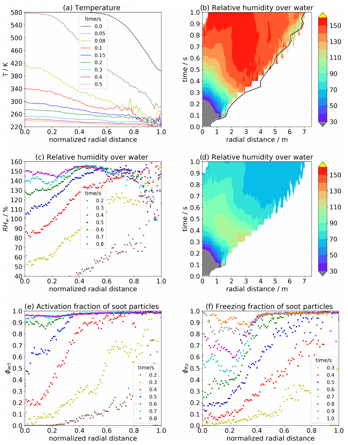
Figure 1Radial profiles of (a) temperature and (b–d) relative humidity over water RHliq in percent, (e) fraction of soot particles activating into water droplets ϕact and (f) freezing to ice crystals ϕfrz. Whereas panels (a–c) show results from a simulation with switched-off contrail microphysics, panels (d–f) show results from the baseline case with switched-on contrail microphysics. The contour plots in (b, d) show RHliq over (r,t) space, where r is the absolute radial distance from the plume centre. The black line in (b) indicates the increasing plume radius rp over time. All other panels show line plots at different plume ages (indicated by the legend), where the horizontal axis uses the normalized radial distance as coordinates.
In the FLUDILES simulation, the initial plume temperature profile is based on the Crocco–Busemann relation (White, 2005) and introduces a smooth radial transition between the plume and the environment. This ensures numerical stability as gradients in prognostic variables that are too strong are numerically intricate. This means that T3D,k(t0) only equals T3D,0 directly behind the nozzle exit centre and decreases down to around 400 K towards the plume edge (see black line in Fig. 1a). These trajectories start with 𝒟k,0<1 and an accordingly higher initial dilution . For simplicity, we mostly neglect this fact in the following description, but the initialization in this transition region is consistently treated in our model.
The process of converting jet kinetic energy into thermal energy is considered within the 3D simulations. This means that the FLUDILES temperature is higher than a “passive tracer temperature”. Therefore, we underestimate dilution, causing a later onset of contrail formation. This effect is partially compensated for by the inhomogeneous initial temperature profile, implying that exhaust air parcels are already diluted near the plume edge.
Basically, we only infer the dilution from the trajectory data according to Eq. (17) and plug the corresponding entrainment rate values into Eqs. (9) and (10) for each trajectory. For the radial plots presented later on, the coordinate data of these trajectories are used, but the actual computations are independent of this type of information.
Note that the ambient temperature Ta and plume temperature at engine exit T0 in Eqs. (9) and (10) are allowed to differ from T3D,a and T3D,0 used in Eq. (17). Similarly, the ambient and initial plume water vapour can be chosen independently of the 3D data. In such a case, we basically only use the information of the dilution and its variability.
Moreover, a single mean state trajectory can be derived from the trajectory ensemble. We determine the corresponding mean dilution 𝒟AT by averaging the preprocessed temperature data over all 25 000 trajectories and plugging the average temperature evolution into Eq. (17).
There are other ways of computing the mean properties of the trajectory ensemble. For instance, the mean temperature can be a weighted average, where the cross-sections or masses of the trajectories are used as weights. The internal energy is conserved when a mass-conserving temperature average is used. The Supplement shows additional results for a mass-conserving temperature average and contrasts them with our default procedure.
2.4 Box model framework
We use the LCM box model, which is based on the 3D LCM (introduced in Sect. 2.1) and has been extended for the contrail formation microphysics. Similarly to Paoli et al. (2008), we either perform a single box model run with an average dilution (labelled “average traj”) or an ensemble of box model runs for the trajectory dilution data (labelled “ensemble mean”). The simulated time tsim is 2 s. In the following, we describe the initial conditions (Sect. 2.4.1) and introduce important diagnostics, including explanations about the averaging procedure for ensemble mean runs (Sect. 2.4.2).
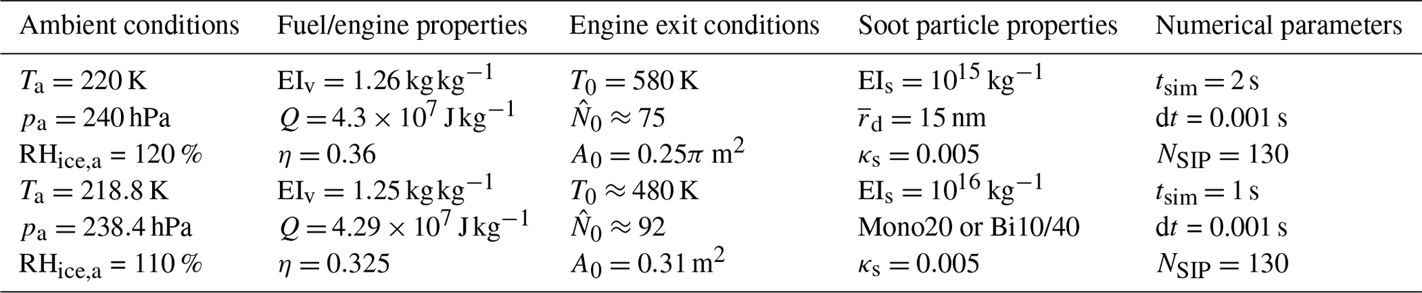
Table 1Baseline parameters of all regular LCM simulations (first three rows) and those corresponding to the box model set-up of Lewellen (2020) (last three rows). Hereby, Mono20 stands for a monodisperse distribution with rd=20 nm and Bi10/40 for a bidisperse distribution with a mixture of 10 and 40 nm particles.
2.4.1 Initial conditions
Table 1 summarizes initial conditions of our baseline scenario, which are described in the following. The plume exit temperature (near the plume centre) is set to 580 K. We prescribe an ambient temperature of either 220 K (baseline case) or 225 K (near-threshold case). The baseline SA threshold temperature (ΘG) is 226.2 K for the given atmospheric conditions and engine/fuel properties. The prescribed ambient relative humidity over ice, RHice,a, determines the ambient water vapour mixing ratio xv,a being proportional to RHice,a⋅es,ice(Ta). We use RHice,a = 120 % for the baseline case.
Engine and fuel parameters such as specific combustion heat, propulsion efficiency and water vapour mass emission index are prescribed consistently with the trajectory data set-up and have values according to an A340-300 aircraft at cruise speed (Table 1). These parameters are kept constant for all sensitivity studies, even though they can slightly change with varying ambient conditions. For the fuel consumption, which is calculated by rearranging Eq. (15), we obtain lower values than typical for this aircraft type since the initial plume radius given by FLUDILES is only 0.5 m (Sect. 2.3.2). For given T0, specific combustion heat and propulsion efficiency, we obtain according to Eq. (13). Note that the initial plume water vapour mixing ratio is controlled by the water vapour emission index EIv:
where the second term is the contribution of ambient humidity entering and exiting the engine. This term is less than 1 % of the total plume water vapour and, therefore, neglected in our initialization.
Based on laboratory measurements, we prescribe log-normally distributed soot particles with a geometric-mean dry core radius () of 15 nm and geometric width of 1.6 (Hagen et al., 1992; Petzold et al., 1999) and set the engine soot number emission index (EIs) to 1015 kg−1 as a typical value for commercial aircraft (e.g. Schumann et al., 2002, 2013; Kleine et al., 2018). Furthermore, we assume the same hygroscopicity parameter value (κs=0.005) as in Kärcher et al. (2015).
The overall number of emitted engine soot particles per flight distance is given by
Table 2Parameter variations (PVs) of various soot properties and ambient conditions. The values in bold depict the default baseline parameter, and EIs,ref is the baseline soot number emission index.
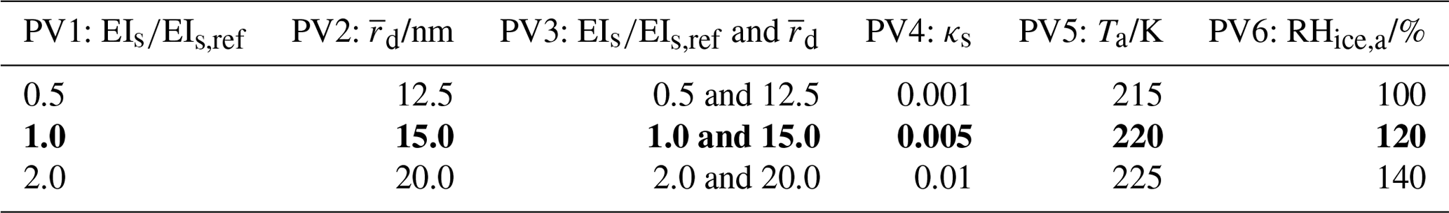
Table 2 summarizes the parameter variations (PVs) that investigate the sensitivity of contrail formation to soot properties (PV1–PV4) and ambient conditions (PV5/PV6). In the first two PVs, we either vary EIs or . Flight measurements have shown that a 50:50 mixing of conventional kerosene with a biofuel causes a decrease in EIs by around 50 % (Moore et al., 2017). Moreover, they find a decrease of the average soot particle size. This is because the switch to alternative fuels leads to a reduced number of primary soot spherules. The subsequent coagulation between those spherules decreases, and the final soot aggregates are smaller on average. Therefore, in PV3, we vary both EIs and and combine a 50 % reduction in EIs with a reduction in to 12.5 nm. In PV4, we change the hygroscopicity parameter of soot particles in a reasonable range between 0.001 and 0.01 (Markus Petters, personal communication, 2019). Finally, we study the variation of contrail properties with ambient temperature Ta (PV5) and relative humidity over ice RHice,a (PV6).
2.4.2 Diagnostics
Here, we introduce diagnostics that are used to evaluate the simulations.
The fraction of soot particles activated into water droplets (ϕact) or frozen to ice crystals (ϕfrz) is given by
where ζi characterizes whether soot particles () represented by a SIP i have turned into water droplets ( and ) or ice crystals (). Note that we classify ice crystals as activated; hence we get .
We introduce the apparent ice number emission index, AEIice, as a measure of the number of formed ice crystals per fuel mass burnt. Since we consider only soot as exhaust particles in our study, AEIice is simply given by the product of ϕfrz and EIs.
Furthermore, we define the effective radius of the soot–droplet–ice number distribution as
Typically, reff is a quantity that is relevant in radiation problems. Here, we prefer reff over the ordinary mean radius since the time evolution is smoother, and there is no need to specify the total particle number.
For ensemble mean values, intensive and extensive physical quantities are mass-weighted averages and sums of trajectory ensemble values, respectively. For quantities that are defined as ratios like the effective radius or relative humidity, first the averages of the quantities that appear in the denominator and nominator are computed, and then the ratio over those averaged quantities is taken. Note that the mass weights cancel out in the definitions of ϕact/frz and reff.
In this section, we first describe the spatio-temporal evolution of thermodynamic and contrail properties during the formation stage (Sect. 3.1). We then analyse the temporal evolution of contrail properties depending on different soot properties and atmospheric parameters in Sect. 3.2. Finally, we summarize our results by studying the sensitivity of final contrail ice crystal numbers to ambient temperature and relevant soot properties. Our simulations are based on the FLUDILES dilution data, and we particularly compare simulations using the full trajectory ensemble and a single average trajectory.
3.1 Spatial variation of contrail properties
The first two rows of Fig. 1 depict the spatio-temporal evolution of temperature and relative humidity. The plume radius (black line in Fig. 1b) is evaluated as the distance of the most remote trajectory from the plume centre at given plume age t. The jet plume expands from an initial radius of 0.5 m towards around 7.5 m after t=1 s. Figure 1a shows the radial profiles of temperature for different plume ages. In the very beginning (black), the plume centre is not affected by entrainment, and the core temperature remains at its initial value. In the outer areas, the temperature profile is smoothed according to the Crocco–Busemann profile. The radial temperature gradient is initially large (nearly a temperature decrease of 300 K at t=0.05 s) and decreases with increasing plume age as the plume centre cools. Later on, the absolute changes in temperature, spatially and temporally, decrease continuously.
Figure 1b shows the radial–temporal RHliq distribution of a simulation with switched-off contrail microphysics, where water vapour behaves like a passive tracer. We call the displayed quantity the hypothetical RHliq; it increases with increasing plume age (at least for t≤0.5 s) and decreasing plume temperature due to the non-linearity of the saturation vapour pressure. Since plume cooling starts earlier and proceeds faster near the plume edge, water saturation is surpassed earlier in this region (after 0.25 s) than in the plume centre (after 0.5 s). For a fixed plume age up to t=0.5 s, the hypothetical RHliq increases with increasing radial distance for as is apparent from Fig. 1c. At higher plume ages and radial distances, the dependency of the hypothetical RHliq on r,t reverses.
Figure 1d–f show results of a simulation with switched-on contrail microphysics. As soon as droplet formation on soot particles is initiated (i.e. after plume relative humidity exceeds at least water saturation), the further increase in RHliq is inhibited due to condensational loss of water vapour. The subsequent rapid decrease in RHliq (first at the plume edge and later on in the plume centre) is due to ice crystal formation and subsequent depositional growth. After around 1 s, the relative humidity with respect to ice reaches values of 100 %, which translates into water-subsaturated plume conditions. Figure 1e shows the fraction of activated soot particles (ϕact). According to the evolution in plume relative humidity, soot particles activate into water droplets first near the plume edge and afterwards in the plume centre. Water saturation in the plume is first reached for Tsat≈240 K so that below those temperatures soot particles may form water droplets and grow further by condensation. The homogeneous freezing of the super-cooled water droplets typically occurs at Tfrz≈ 230–232 K depending on the droplet size and the cooling rate. Figure 1f shows the fraction of soot particles that turned into ice crystals (ϕfrz). The radial profiles of ϕfrz behave similarly to the corresponding profiles of ϕact but with a time lag of around 0.2 s. In the outer part with , basically all soot particles have become ice crystals after around 0.6 s. At t = 0.6–0.8 s, the profiles exhibit local minima at , which results from the minimum in RHliq after around 0.7 s (Fig. 1b).
3.2 Temporal evolution of contrail properties
3.2.1 Mean state trajectory versus trajectory ensemble
We employ the box model in two different frameworks as outlined in Sect. 2.4. In the average traj framework, a single box model run with an average dilution is performed. In the ensemble mean framework, box model runs are carried out for the complete set of 25 000 trajectories.
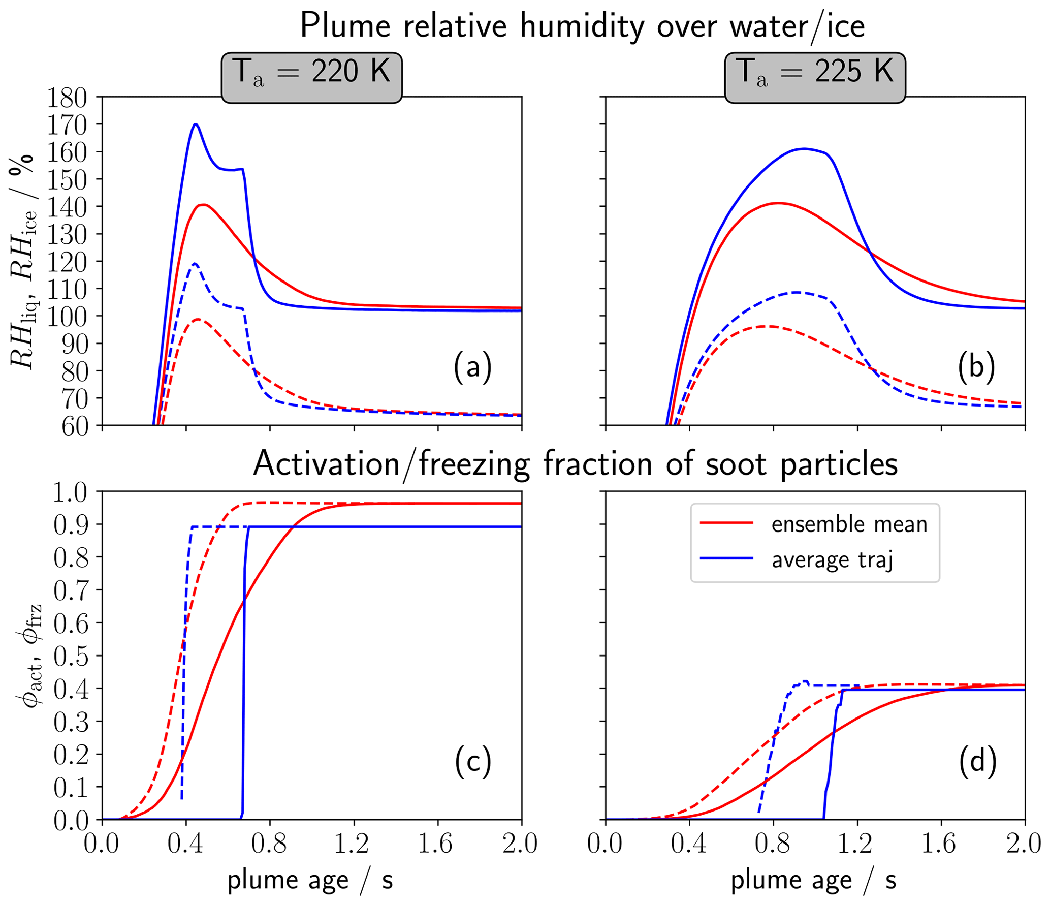
Figure 2Temporal evolution of (a, b) plume relative humidity over water (dashed) and ice (solid) and of (c, d) the fraction of soot particles activating into water droplets (dashed) and forming ice crystals (solid). The left column (a, c) shows the baseline case with ambient temperature Ta=220 K and the right column (b, d) the near-threshold case with Ta=225 K. Results are shown for the ensemble mean (red) and the average traj (blue) evolution.
Figure 2 compares the plume relative humidity (top row) and the activation–freezing fraction between both frameworks. This is done for baseline conditions (Fig. 2a and c, Ta = 220 K) and a near-threshold case (Fig. 2b and d, Ta = 225 K with 1.5 K). First, we analyse the baseline case. For the average traj, RHliq surpasses water saturation after around 0.4 s and leads immediately to a rapid droplet formation on soot particles. Thereby, ϕact increases quasi pulse-like from zero to its final value. Subsequently, RHliq decreases and approaches 100 %. After 0.7 s the droplets freeze rapidly into ice crystals, and the depositional ice crystal growth causes a steeper decrease in RHliq until ice saturation is reached (see blue line in Fig. 2a). Regarding the ensemble mean evolution, the fraction of soot particles forming droplets/ice crystals increases smoothly over a certain time window. This is explained as follows: the spatial variability in RHliq is quite large (Fig. 1d) due to a systematic radial gradient and superposed turbulent deviations. Therefore, droplet and ice crystal formation occurs for different trajectories at a different plume age, mostly depending on the radial distance to the plume centre (Fig. 1e and f). Although the ensemble mean features a smaller RH peak value than the average traj evolution, a larger fraction of soot particles forms ice crystals (96 % vs. 88 %).
In the near-threshold case (right column), Tsat≈ 236 K is lower and closer to Ta. Hence, water saturation is reached at a higher plume age when the cooling rates are already lower. Additionally, the peak RH values are clearly reduced. According to the evolution of the plume relative humidity, droplet and ice crystal formation on soot particles is initiated a few tenths of a second later compared to Ta = 220 K ((Fig. 1d). The time between the activation of the first droplets and the freezing of the last droplets is also longer (1.6 versus 1.2 s). The final ϕact and ϕfrz values are clearly reduced relative to the baseline case since only the larger soot particles can activate into water droplets due to the decreased peak RHliq. Again, the ensemble mean evolution displays slightly higher final ϕfrz values than the average traj.
A closer look at the average traj evolution of the near-threshold case reveals that ϕact is not a monotonically increasing function and that the final ϕfrz value is lower than the ϕact value at some intermediate time (in this example at t=0.9 s). This is explained as follows: the largest soot particles are activated first, and over time smaller soot particles grow large enough to be considered activated as well. However soon after, RHliq drops below SK (for the smaller soot particles) as condensational growth removes water vapour. Those particles shrink, such that their radius drops below the activation radius. Once the largest water droplets freeze, depositional growth leads to a fast depletion of water vapour. Again, the smallest of the currently activated droplets face water-subsaturated conditions and also become deactivated (at around t=1.25 s). We will encounter this “deactivation phenomenon” later again. Even though it is not visible in the ensemble mean evolution, this deactivation phenomenon also occurs for most trajectories of the ensemble runs.
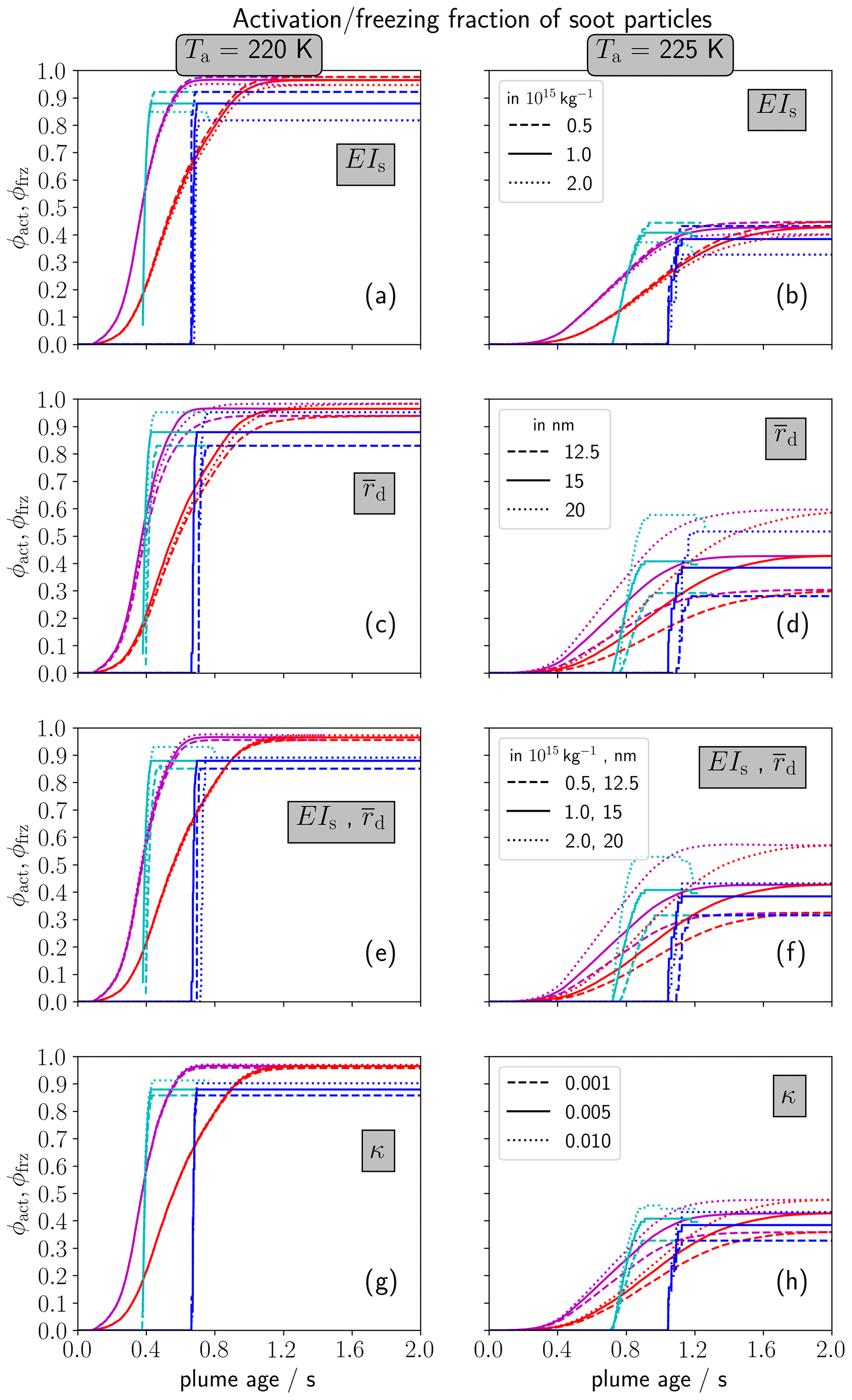
Figure 3Temporal evolution of the fraction of soot particles activating into water droplets ϕact (cyan and magenta) and forming ice crystals ϕfrz (blue and red) for a variation of the soot number emission index EIs (a, b), geometric-mean dry core radius (c, d), a combined variation of EIs and (e, f) and a variation of the hygroscopicity parameter κ (g, h). The left column (a, c, e, g) shows the baseline (Ta = 220 K) and the right column (b, d, f, h) a near-threshold case (Ta = 225 K). The magenta and red lines show the ensemble mean and the cyan and blue lines the average traj results. The different line types (see legends on the right column) represent the according soot parameter variations (PV1–PV4).
3.2.2 Variation with soot properties
In this section, we investigate the sensitivity of contrail formation to various soot properties. Figure 3 presents results of the sensitivity studies PV1 to PV4. As in the previous section, the baseline and near-threshold temperature cases are considered. We first analyse the baseline temperature case (Ta=220 K; Fig. 3a, c, e and g). The ensemble mean results reveal that the temporal evolution of the activation fraction ϕact and freezing fraction ϕfrz hardly changes with any variation of the soot properties. In the average traj framework, the sensitivity to soot properties is slightly higher. There, the activation and freezing fraction moderately increases with decreasing EIs (Fig. 3a) and increasing (Fig. 3b). A higher number of soot particles leads to a faster depletion of plume relative humidity, prohibiting the activation of smaller particles. Likewise, a decrease of reduces the number of soot particles that manage to be activated. Changing the two parameters, EIs and , simultaneously (Fig. 3c), the effects on ϕact and ϕfrz more or less cancel out, resulting in an almost negligible effect. The variation of ϕfrz with the hygroscopicity of soot particles (Fig. 3d) displays the lowest impact within the considered parameter range. Note that the average traj simulations with higher prescribed EIs (dotted cyan lines) exhibit the aforementioned deactivation phenomenon.
In the near-threshold scenario, the ϕact and ϕfrz values are clearly lower due to decreased plume water supersaturation (Sect. 3.2.1). While the variation with EIs (Fig. 3b) is still low, both average traj and the ensemble mean evolution are more sensitive to the variation of and κ than for Ta=220 K. This is because of two basic reasons: first, the critical saturation ratio for the activation of soot particles varies non-linearly with the soot core size (due to the non-linear Kelvin term), displaying a strong change for rd<10 m (Fig. B1a). This means that far away from the formation threshold, larger changes of and κ are necessary to affect the activation of the several nanometre-sized soot particles. Second, these small soot particles are at the tail of the size-distribution, and, therefore, their activation only makes a low contribution to the overall ϕact. In the near-threshold case, only the larger soot particles (rd≳20 nm) can form water droplets. This activation threshold is close to , which simultaneously defines the maximum of the log-normal size distribution. Hence, changing or κ has a significantly higher impact on ϕact for Ta=225 K than for lower ambient temperature.
Again, we find a stronger sensitivity to rd (Fig. 3d) than for κ (Fig. 3h) Interestingly, the ensemble mean simulations show larger rd- and κ-induced variations in ϕfrz in the end than the average traj simulations, which is opposite to what we saw in Fig. 3c and g. This is mainly due to the deactivation phenomenon. In the combined variation of EIs and (Fig. 3f), the impact of on ϕact and ϕfrz dominates over that of EIs. Halving the EIs value and decreasing to 12.5 nm leads to a decrease in ϕfrz from 0.41 to 0.31 and translates into a decrease of AEIice even by 62 % (instead of around 50 % if only the EIs value is halved).
Furthermore, we have investigated the sensitivity of contrail formation to the geometric width of the soot particle size distribution σ (not shown): in contrast to the variation with and κ, there is a negligible impact near the contrail formation threshold (Ta = 225 K). This is because the activation of soot particles with dry core radii below is already inhibited due to the Kelvin effect. For our baseline case, a higher fraction of soot particles forms ice crystals if the geometric width is reduced. This is due to the fact that the smallest soot particles within the size distribution become larger and hence can be activated more easily. Decreasing (increasing) geometric width from 1.6 to 0.8 (2.4) causes a decrease (increase) in ϕfrz from 0.88 to 0.83 (0.98) for the average traj and from 0.96 to 0.93 (0.99) for the ensemble mean.
3.2.3 Sensitivity to ambient conditions
In this subsection, we study the dependence of contrail formation on ambient conditions. We vary the ambient temperature Ta and background relative humidity over ice RHice,a (see PV5 and PV6 in Table 2).
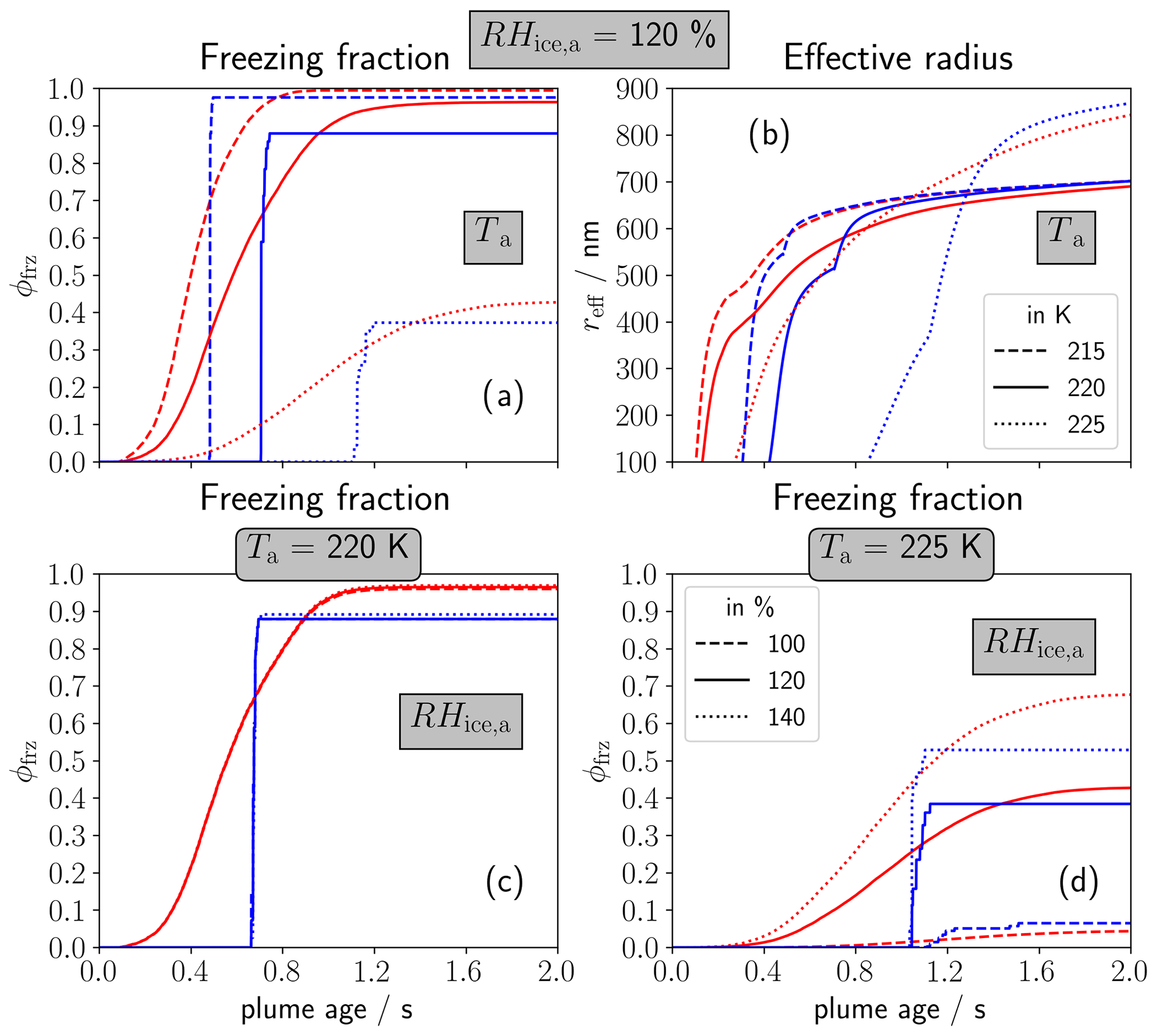
Figure 4Temporal evolution of the freezing fraction of soot particles ϕfrz (a, c, d) and effective radius reff (b) for a variation of ambient temperature Ta (a, b) and RHice,a (c, d) according to the inserted legends in the right column. The variation of RHice,a is shown for two different Ta values (see panel titles). The red lines show the ensemble mean and the blue lines the average traj results.
Figure 4a and b display the variation of ambient temperature Ta at default RHice,a=120 %. As already explained above, a change of Ta affects the contrail formation time and the number of soot particles turning into ice crystals. The lower the Ta, the earlier that water saturation is first reached in the plume and the higher the attained peak water supersaturation is. Hence, reducing Ta to 215 K, droplet and ice crystal formation is initiated earlier, and more ice crystals form (Fig. 4a). The results for Ta=220 and 225 K have already been described in Sect. 3.2.2. Thereby, the difference in ϕfrz is significantly larger between 225 (dotted) and 220 K (solid) than that between 220 and 215 K (dashed).
The evolution of the effective radius reff in Fig. 4b shows a steep increase from the moment when the first droplets are activated. The increase slows down in most cases and is accelerated again once the droplets freeze. The curves level off as soon as ice saturation is reached in the plume. This happens after around 1 s for the lower Ta and after around 2 s for Ta=225 K. The final reff values hardly change between Ta=215 and 220 K and between the average traj and the ensemble mean. Only for Ta=225 K are higher values attained. This is because the absolute amount of ambient water vapour is higher for higher Ta and gets distributed among fewer ice crystals.
Figure 4c and d show the variation of RHice,a. For Ta=220 K (Fig. 4c), contrail ice nucleation is not at all affected by the variation of RHice,a. In contrast, the sensitivity of ϕfrz to RHice,a is very high for Ta=225 K. At ice saturation (dotted line), only few ice crystals form (ϕfrz<10 %). This is because a decrease in RHice,a causes a decrease in ΘG from 226.2 to 225.5 K so that those contrails form only 0.5 K below the SA threshold temperature, and maximum plume water supersaturation is only a few percent. Analogously, more ice crystals form for RHice,a=140 % as ΘG, and hence K is higher.
Our results highlight that the sensitivity of contrail ice nucleation to atmospheric parameters is large near the contrail formation threshold, which is consistent with previous studies (e.g. Kärcher and Yu, 2009; Kärcher et al., 2015; Bier and Burkhardt, 2019). Therefore, it is meaningful to display the variation of the nucleated contrail ice crystal number with as well (see next section).

Figure 5Fraction of soot particles freezing to ice crystals ϕfrz,f (a, c and e) and apparent ice number emission index AEIice,f (b, d and f) at a plume age of 2 s depending on EIs (a, b), ambient temperature Ta in panel (c) (where the axis on the top additionally shows the temperature difference to the SA threshold, ) and on the geometric-mean soot core radius in panels (d–f). In all but panel (c), results are shown for Ta of 220 K (solid) and 225 K (dashed), indicated by the legend in the top right panel. In panel (d), EIs is fixed to the baseline case, while in panels (e) and (f), the total soot mass is fixed (implying an adaptation of ). The red lines show the ensemble mean and the blue lines the average traj results.
3.3 Final ice crystal number
In the following, we aim at summarizing the results from the previous sensitivity studies. We analyse the sensitivity of final contrail ice crystal numbers to ambient temperature and relevant soot properties. Thereby, we display both the freezing fraction (Fig. 5a, c and e) and the absolute ice crystal number in terms of AEIi,f (Fig. 5b, d and f). The latter is shown only for sensitivities with varying EIs since otherwise there is simply a linear relationship between ϕfrz,f and AEIi,f.
The freezing fraction in general decreases with increasing EIs (Fig. 5a) because the plume humidity is depleted faster at higher exhaust particle number concentrations and also distributed among more ice crystals. Hence, the smaller soot particles do not manage to form contrail ice crystals. In our model set-up, the ensemble mean ϕfrz,f only slightly changes with EIs, confirming the low sensitivity pointed out in Sect. 3.2.2. Accordingly, the ensemble mean AEIi,f increases nearly linearly with increasing EIs. The average traj ϕfrz,f evolution (blue curve) features a stronger decrease than the ensemble mean, in particular for the higher soot number emissions (EIs>1015 kg−1). This is due to the deactivation phenomenon explained in Sect. 3.2.2. Therefore, the increase in AEIi,f with rising EIs flattens in the average traj case.
Figure 5c displays the variation of ϕfrz,f with ambient temperature Ta (lower label) and the difference between Ta and ΘG (ΔT, upper label). Note that the relation between Ta and ΔT is not purely linear since the ambient relative humidity over water varies with Ta at fixed RHice,a, and, hence, ΘG slightly changes as well. Near the contrail formation threshold (i.e. |ΔT|≲ 3–4 K), ϕfrz,f strongly increases with rising |ΔT|. This is because the maximum plume water supersaturation increases, and more and more soot particles manage to activate into water droplets. Below Ta=220 K (|ΔT|>6 K), more than 90 % of the soot particles turn into ice crystals for our parameter setting so that AEIi,f approaches EIs. The average traj simulation produces somewhat lower ϕfrz,f values than the ensemble mean simulation. Furthermore, low soot simulations (with EIs reduced by 80 % relative to the baseline case) feature a similar evolution in ϕfrz,f and a smaller difference between the average traj and the ensemble mean (not shown).
Finally, we investigate the contrail formation dependence on the soot particle size, as specified by the geometric-mean soot dry core radius . Figure 5d shows a variation with for fixed baseline EIs. At Ta=220 K (solid lines), nearly all soot particles can form ice crystals as long as is larger than 20 nm. For smaller mean dry core radii, ϕfrz,f starts to decrease. This decrease is stronger for the average traj (blue vs. red curve). Near the formation threshold (dashed), ϕfrz,f values are clearly lower. Again, the ensemble mean values are larger than the average traj values. Moreover, we see a strong dependence on over the full parameter range.
In the third row of Fig. 5, is varied together with EIs such that the overall soot mass is fixed. We find a qualitatively similar evolution in ϕfrz,f compared to the previous sensitivity study (Fig. 5d) so that the impact of dominates. Yet, AEIi,f (Fig. 5f) is controlled by the change in EIs (EIs decreases with increasing ), and the trend is opposite to that in Fig. 5d.
The following evaluation of our box model computations relies on the comparison with other contrail formation simulations. Generally, such model simulations can differ in various aspects, which we group into four categories: the initial and ambient conditions, the prescribed dilution, the model (micro)physics and the model framework (average traj, ensemble mean or fully 3D LES). If simulations have different settings or properties in several or all four categories, a comparison can hardly be conclusive as differences in the simulation results can have more than one origin. Hence, we made efforts to reproduce the simulation set-up of the recent study by Lewellen (2020, abbr. as Lew20 hereinafter) by using his baseline conditions (more specifically those used in his Fig. 2). They differ from our baseline conditions as summarized in our Table 1. The most significant differences are certainly the factor 10 difference in the EIs value and the shape of the soot size distribution. Lew20 either uses a monodisperse soot size distribution with rd=20 nm or a bidisperse distribution with a 50/50 mixture of rd=10 nm and 40 nm soot particles. Moreover, Lewellen was so kind to provide the dilution data that he used in his box model simulations and the simulation data depicted in his Fig. 21. This enables us to perform simulations with very similar settings, basically in all the four categories mentioned above. In particular, the microphysical treatment of contrail formation is very similar in our approach that includes the transient liquid phase.
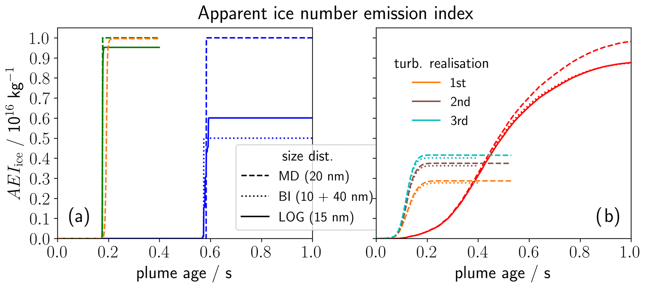
Figure 6Temporal evolution of the apparent ice number emission index under baseline conditions of Lewellen (2020, “Lew20”) as summarized in the bottom half of Table 1. The simulation initialization uses a monodisperse (dashed), bidisperse (dotted) or log-normal (solid) size distribution of soot particles (see also inserted legend). Panel (a) juxtaposes the FLUDILES based average traj evolution (blue) with the evolution using Lew20's dilution (green) and with the results of Lew20's box model (orange). Lew20's data are available up to a plume age of 0.4 s. Note that the dashed and dotted green lines are mostly covered by the solid green line. Panel (b) depicts the FLUDILES ensemble mean evolution (red lines) with the LES results from Lew20's Fig. 2 for three different turbulent realizations (remaining colours).
Figure 6 shows different types of simulations that all use the baseline conditions of Lew20. We first discuss the average traj box model simulations in Fig. 6a. The selection of the simulations serves two purposes: first, applying two different dilution data sets in our LCM model highlights the impact of the dilution data (green vs. blue lines). Second, the LCM simulations using Lew20's dilution data are compared to the box model simulations of Lew20 (green vs. orange lines). This aims at validating the microphysical approach and implementation in both models. Results are presented for a monodisperse and bidisperse (as in Lew20) as well as for our regular log-normal soot size distribution. All simulations feature a pulse-like increase in AEIice once freezing starts. However, ice crystal formation is initiated significantly earlier for Lew20's dilution, namely after 0.25 s instead of 0.6 s for the FLUDILES dilution. One reason for that is the FLUDILES dilution being too weak since temperature is treated as a passive tracer (Sect. 2.3). Another aspect of physical nature is our higher initial plume radius (i.e. 0.5 m instead of 0.3 m in Lew20), causing the jet plume to dilute on a longer timescale. Lew20 analysed the effects of increasing engine size and found significant impacts on contrail ice crystal formation, particularly for higher aerosol number emission indices (see his Figs. 13 and 14).
Using the bidisperse soot initialization (dashed blue), we find AEIice=0.5EIs for the FLUDILES dilution as the 10 nm soot particles are not activated into water droplets. Yet, all soot particles are activated for Lew20's dilution. This is remarkable as for both dilution data the maximum plume water supersaturation would be the same if the microphysical processes were suppressed. The reason for the different activation fraction is that the time period between droplet formation and freezing is longer, and correspondingly also the cooling rates are lower within this period in the FLUDILES case. This leads to a reduced peak saturation ratio, which is smaller than the critical saturation ratio for the activation of the 10 nm particles.
For the log-normal size distribution (solid blue), some smaller soot particles are only temporarily activated but then shrink again as the larger droplets originating from the larger soot particles deplete water vapour. With Lew20's dilution (solid green), there is not enough time between activation and freezing to deactivate the smaller droplets. This difference originating from the different dilution data implies that the deactivation phenomenon, which we frequently encountered in our results, may not occur that frequently if plume cooling proceeds faster. Further implications concerning this aspect will be discussed in Sect. 5.
As a next step, we compare our box model simulations using Lew20's dilution (green) with Lew20's box model simulation (orange). From the latter model only results for the monodisperse soot initialization are available, yet the bidisperse case gives basically identical results. We find a perfect agreement between both models with an only some hundredth of seconds earlier increase in AEIice for the LCM. (Note that the dashed and dotted green lines are mostly covered by the solid line). This is because our freezing temperature (Tfrz) is slightly higher than that of Lew20 (David Lewellen, personal communication, 2020), leading to an earlier onset of ice crystal formation.
Figure 6b displays FLUDILES ensemble mean simulations (red lines) and 3D LES results with online coupled microphysics of Lew20. The latter are shown for three different turbulence realizations, demonstrating irreducible uncertainty involved in predicting contrail formation. The ice crystal number from the 3D LES is not only considerably reduced relative to our AEIice, but also relative to the box model framework of Lew20 using the same microphysics as in his 3D LES. Lewellen explains this as follows: “Different parcels in the plume produce ice crystals at different times. As these parcels interact via mixing, the moisture consumption from early crystal growth in some parcels can prevent the activation and freezing of soot aerosol in other parcels that later mix in. … Thus, the much narrower time window for ice number production seen in the box model leads to greater EIiceno [AEIice] than in the LES.”
Originally, we supposed that switching from the average traj to the ensemble mean framework leads to more realistic quantitative results as already assumed in Paoli et al. (2008). However, we see an opposite trend compared to the 3D LES, namely the ice crystal number rises when we switch from the average traj (blue lines in left panel) to the ensemble mean (red lines in right panel). We believe this comes from the fact that we do not consider the inter-trajectory mixing mentioned above. This means that offline ensemble simulations miss an important process, and their quantitative prediction of AEIice is not more reliable than from an average traj simulation, even though they account for plume heterogeneity and are in several aspects more plausible. Note that the reasoning above is based on comparing only a few simulations. For instance, Lew20 shows that for EIs≤1015, all soot particles form ice crystals in the LES (see his Figs. 5 and 11), and hence there is no longer a difference between Lew20's average traj and LES predictions of AEIice. Moreover, the deactivation phenomenon leading to the large difference between FLUDILES average traj and ensemble mean results may be exaggerated with the FLUDILES dilution. This implies that the difference between the average traj and the ensemble mean could be smaller with a stronger dilution. We test this hypothesis in the following discussion section.
Similar to our study, Paoli et al. (2008) compared average traj and ensemble mean results for two specific parameter settings. They also used a set of 25 000 trajectories, even though it is not the same data set provided by Vancassel et al. (2014). Several aspects are similar to ours, for example, the quasi pulse-like activation versus a formation period. Interestingly, they find that for the average traj, the final ice crystal number is even 3 times lower than for the ensemble mean.
In the previous section, we have shown that ice crystal formation is initiated significantly earlier, and the number of formed ice crystals may be even larger if we use Lew20's data instead of the FLUDILES dilution data. Furthermore, we stressed that some differences found between the ensemble mean and the average traj results may be particularly due to too weak a dilution. In the following, we will estimate the time lag of the plume mixing and discuss potential improvements in our results by “accelerated” trajectory data.
While 38 % of the total combustion energy Etot is used for the propulsion of the aircraft (according to the A340-300 propulsion efficiency), the remaining energy (62 %) is transferred into the jet plume in the form of kinetic energy Ekin and thermal energy Etherm. For the initial partitioning, we assume that Etherm is in the range 51 %–31 % of Etot, and, accordingly, . During the jet expansion, Ekin is continuously converted into Etherm, leading to a temperature excess relative to a passive tracer temperature. Based on 3D simulations with EULAG, we estimate that around 90 (95 %) of Ekin is already converted into Etherm after 0.4 s (0.8) s of plume age. Calculating the temperature excess, our estimated time lags are 0.05–0.15 s after 0.4 s, 0.1–0.25 s after 0.6 s and 0.15–0.35 s after 0.8 s of plume age. Note that the lower/upper time lag limit refers to the smallest/largest assumed initial jet kinetic energy.
In the following, we introduce a small correction to “speed up” our existing trajectory ensemble. More specifically, we artificially increase the dilution rate of each FLUDILES trajectory such that in the end the average dilution of this corrected trajectory ensemble, 𝒟AT,F2L, matches the dilution of Lew20, 𝒟AT,Lew20. At each time step, we diagnose , where 𝒟AT,FLUDILES is the average dilution defined at the end of Sect. 2.3, and “F2L” stands for “FLUDILES to Lewellen”. For each trajectory of the existing database, we use a modified dilution evolution defined as . It is easy to show that the average traj dilution 𝒟AT,F2L of the modified trajectory ensemble equals 𝒟AT,Lew20.

Figure 7Final freezing fraction of soot particles against (a) soot number emission index and (b) ambient temperature (where the axis on top additionally shows the temperature difference to the SA threshold ΔT). We juxtapose the original FLUDILES trajectory ensemble (red) with the sped-up ensemble (magenta), whose average dilution matches that of Lewellen (2020). The blue and green lines show the corresponding average traj evolution of both ensembles. Additionally, the results from the parameterization of Kärcher et al. (2015) with an adaption regarding the calculation of the activation dry core radius of soot particles (brown) are shown.
Figure 7 shows the sensitivity of the final freezing fraction of soot particles (ϕfrz,f) to (a) EIs and (b) Ta for the original FLUDILES simulations (blue and red lines, as already depicted in Fig. 5a and c) and for the sped-up scenario (green and magenta) according to Lew20. We are particularly interested in comparing the evolution between the ensemble mean and the average traj. In terms of the EIs sensitivity, the difference between the two frameworks is apparently smaller in the sped-up scenario than in the original data set. Considering the variation with Ta, the original average traj displays the lowest ϕfrz,f (blue) of all other simulations since the deactivation phenomenon leads to fewer ice crystals. For the sped-up scenario, the difference between the ensemble mean and the average traj is again significantly lower than for the original data set. Both sensitivity scenarios confirm our hypothesis that the weak dilution of the original data is conducive to excessive deactivation in the average traj set-up. Furthermore, the ice crystal number is in general higher for the sped-up scenario (magenta) than for the original data set (red).
Additionally, we show the results of the parameterization by Kärcher et al. (2015) in an adapted version. This parameterization was recently implemented in a global climate model (Bier and Burkhardt, 2019), where it refines the contrail initialization procedure. Those results (brown lines in Fig. 7) lie well in the range of the other simulations results. Overall, the extensive evaluation may help interpreting previous studies based on an average traj or a trajectory ensemble approach.
In this paper, the particle-based Lagrangian Cloud Module (LCM; Sölch and Kärcher, 2010) has been extended to cover the specific microphysics of contrail formation. One of our objectives was to test the newly extended LCM model in a simple box model framework prior to its coupling to the 3D LES model EULAG. Furthermore, our aim was to analyse the most relevant sensitivities of contrail ice crystal numbers to various soot properties and ambient conditions and to compare our results with previous studies.
We employ a data set with dilution histories along 25 000 trajectories sampling the expanding jet. These data are provided by 3D FLUDILES simulations behind the engine nozzle of an A340-300 aircraft (Vancassel et al., 2014). We compare a single box model run with an average dilution with an ensemble mean of box model runs for all dilution histories.
Plume mixing leads to a strong cooling at the plume edge where water saturation is reached first. Later on, also the plume centre cools. Therefore, soot particles form water droplets (and subsequently freeze into ice crystals) first near the plume edge and afterwards in the plume centre.
Consistent with previous studies (e.g. Kärcher and Yu, 2009; Kärcher et al., 2015; Bier and Burkhardt, 2019), contrail ice crystal number varies strongly with atmospheric parameters (like ambient temperature and relative humidity) near the contrail formation threshold. Thereby, the difference between the ambient and Schmidt–Appleman threshold temperature is of relevance since it controls the maximum plume water supersaturation in terms of pure thermodynamics.
Investigating the impact of soot properties on contrail evolution, we find that the fraction of soot particles freezing to ice crystals significantly changes with mean size and solubility of the soot particles only near the contrail formation threshold. This is due to the combined effect of the non-linear Kelvin term and the log-normal soot particle size distribution. The freezing fraction displays a slight decrease with increasing soot number emission index, particularly for higher soot emission levels. This weakens the increase of absolute ice crystal numbers with increasing soot number. To investigate the impact of current biofuel blends, we analyse a combined variation of the soot number emission index and the average soot core radius. We find that the decrease in contrail ice crystal number does not only result from the reduced soot particle number but also from the smaller soot particle sizes.
We evaluate our study with results from a recent study of Lewellen (2020), who uses a similar contrail formation microphysics with a transient liquid phase. Prescribing the same initial and ambient conditions, we particularly find a later onset of contrail formation in our model. This is because our dilution is too weak as discussed in the previous section. When employing the dilution data provided by Lewellen (2020), our evolution in contrail ice crystal number agrees well with the box model results of Lewellen (2020). This suggests correct implementations of the microphysics in both models.
Switching from a single trajectory to the ensemble mean framework shows only an improvement in terms of a smoother (instead of pulse-like) evolution in contrail ice nucleation. On the other hand, we see an increase in final ice crystal numbers, which is, at least for high soot number emissions, an opposite trend compared to the recent 3D LES results of Lewellen (2020). This is likely due to the fact that we do not consider the interaction (mixing and depletion of water vapour) between the different trajectories. Therefore, we overestimate ice crystal formation mainly for high soot particle numbers. Hence, using a large spatially resolving trajectory ensemble does not necessarily lead to improved scientific results, contrary to what we expected in the beginning.
The presented aerosol and microphysics scheme describing contrail formation is of intermediate complexity and thus suited to be incorporated within 3D simulations (LES) of contrail formation explicitly simulating the jet expansion. Our next task is to extend the EULAG-LCM model system, which has been extensively used for high-resolution contrail simulations during the vortex and dispersion phase, by the specific contrail formation physics.
To improve the accuracy of model outputs and to enable a better evaluation with in situ campaign data, contrail formation experiments should include in addition to total number concentrations measurements of exhaust and ice particle size distributions. Due to the large spatial heterogeneity and fast change of thermodynamic and microphysical quantities, a precise determination of contrail age and sampling position in the plume is crucial. High-resolution measurements of water vapour can help to characterize the growth and sublimation of ice crystals. A thorough discussion of benefits and limitations of different measurement strategies is valuable to understand how a quantitative comparison of modelled and measured data should be performed.
A1 Condensational growth
The binary diffusion coefficient of air and water vapour Dv is calculated as (Pruppacher and Klett, 1997)
with p0 = 1013.25 hPa denoting the standard surface pressure and Tmlt=273.15 K the equilibrium freezing temperature over pure ice water. The equation is actually valid for 233.15 K K, but we use it for lower temperatures as well. The heat conductivity of air is approximated as a function of temperature (Jacobson, 1999):
and the specific latent heat for condensation/evaporation Lc is obtained from the equation of Rogers and Yau (1996):
If droplet radii are initially small, i.e. with a magnitude comparable with the molecular mean free path, the condensational growth in the transition regime has to be considered. We use the correction terms for the mass and heat term in Eq. (2) according to Fuchs and Sutugin (1971):
where and b2=0.377 are empirical constants. The Knudsen number (Kn) describes the ratio between the mean free path of the surrounding gas molecules and the droplet radius so that
The mean free paths of vapour (λv) and air molecules (λa) are given by Williams and Loyalka (1991):
with Rd and Rv denoting the specific gas constants for dry air and vapour, respectively.
αm,c and αt,c are the mass and thermal accommodation coefficients for condensation. Here, we set both parameters to unity since droplet growth rates from cloud model studies agree best with experimental studies when choosing these values (Laaksonen et al., 2005).
A2 Depositional growth
The specific latent heat for deposition/sublimation is approximated according to Rogers and Yau (1996):
The transitional correction factors that appear in Eq. (7) are given by Pruppacher and Klett (1997):
where ρa and cp are mass density and specific heat constant of dry air, and αm,d and αt,d represent the mass and thermal accommodation coefficients for deposition, respectively. In this study, we set αm,d to 0.5 according to Kärcher (2003) and αt,d to 0.7.
B1 Calculation of surface tension
For the liquid water droplets formed on soot particles, we assume the surface tension of pure water droplets (σ:=σw). We neglect the impact of dissolved acids on surface tension because the soot-coating substances (like sulfuric acid) make up only a few percent of the overall soot particle/droplet volume (e.g. Petzold et al., 2005). We use the polynomial approximation based on experimental investigations by Hacker (1951) and as reported in Pruppacher and Klett (1997):
which is valid for a temperature range 228.15 K < T < 273.15 K. The coefficients are a0=75.93, a1=0.115, a2=0.06818, , , and .
For ice crystals, we fix the surface tension to 0.106 Jm−2 according to Pruppacher and Klett (1997).
B2 Determination of the Köhler curve maximum
As introduced in Sect. 2.2.3, the Kappa–Köhler equation is given by (Petters and Kreidenweis, 2007)
To obtain the critical saturation ratio for activation of soot particles into water droplets (Sc), we search for the local maximum of SK, which requires to be zero. The root rc is called the critical radius for activation. Substituting and yields
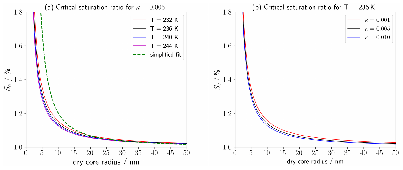
Figure B1Critical saturation ratio (Sc) for the activation of soot particles against dry core radius for different (a) plume temperatures and (b) the hygroscopicity parameter. The dashed line in (a) depicts the evolution of Sc for the simplified Eq. (10) of Petters and Kreidenweis (2007) which is valid for κ≥0.1.
The determination of rc requires the nominator of the first term
to be zero. We solve this numerically and apply a Newtonian iteration until the root rc is determined with an accuracy of < 0.01 nm.
Figure B1a shows that Sc increases with decreasing rd due to the Kelvin effect. The variation of Sc with temperature T is quite low for the range where activation in exhaust plumes typically occurs (see legend). Using the simplified Eq. (10) of Petters and Kreidenweis (2007) (green line) causes a significant overestimation of Sc for rd<15 nm. The critical saturation ratio increases with decreasing hygroscopicity parameter κ due to the solution effect (Fig. B1b).
The presented data are available from the corresponding author upon request (andreas.bier@dlr.de).
The supplement related to this article is available online at: https://doi.org/10.5194/acp-22-823-2022-supplement.
AB and SU conceptualized the methodology, advanced and extended the model code and investigated the data output. AB wrote the first draft of the manuscript, performed the simulations and created the tables and figures. SU evaluated the results. XV provided the FLUDILES trajectory data. All authors wrote, revised and edited the manuscript.
The contact author has declared that neither they nor their co-authors have any competing interests.
Publisher's note: Copernicus Publications remains neutral with regard to jurisdictional claims in published maps and institutional affiliations.
The scientific work has been funded by the Deutsche Forschungsgemeinschaft (DFG) within the project “BI 2128/1-1”.
We thank David Lewellen for providing us with simulation and dilution data published in Lewellen (2020) and his constructive review comments, and we thank Klaus Gierens for his internal review.
This research has been supported by the Deutsche Forschungsgemeinschaft (grant no. BI 2128/1-1).
The article processing charges for this open-access publication were covered by the German Aerospace Center (DLR).
This paper was edited by Martina Krämer and reviewed by David Lewellen and one anonymous referee.
Agarwal, A., Speth, R., Fritz, T., Jacob, S., Rindlisbacher, T., Iovinelli, R., Owen, B., Miake-Lye, R., Sabnis, J., and Barrett, S.: SCOPE11 method for estimating aircraft black carbon mass and particle number emissions, Environ. Sci. Technol., 53, 1364–1373, https://doi.org/10.1021/acs.est.8b04060, 2019. a
Anderson, E. B., Cofer, R. W., Bagwell, D. R., Barrick, J. W., Hudgins, C. H., and Brunke, K. E.: Airborne observations of aircraft aerosol emissions 1,Total nonvolatile particle emission indices, Geophys. Res. Lett., 25, 1689–1692, 1998. a
Barrett, J. C. and Clement, C. F.: Growth rates for liquid drops, J. Aerosol Sci., 19, 223–242, https://doi.org/10.1016/0021-8502(88)90225-X, 1988. a
Bier, A. and Burkhardt, U.: Variability in Contrail Ice Nucleation and Its Dependence on Soot Number Emissions, J. Geophys. Res., 124, 3384–3400, https://doi.org/10.1029/2018JD029155, 2019. a, b, c, d
Bier, A., Burkhardt, U., and Bock, L.: Synoptic Control of Contrail Cirrus Life Cycles and Their Modification Due to Reduced Soot Number Emissions, J. Geophys. Res., 122, 11584–11603, https://doi.org/10.1002/2017JD027011, 2017JD027011, 2017. a
Bock, L. and Burkhardt, U.: Reassessing properties and radiative forcing of contrail cirrus using a climate model, J. Geophys. Res., 121, 9717–9736, https://doi.org/10.1002/2016JD025112, 2016. a
Bock, L. and Burkhardt, U.: Contrail cirrus radiative forcing for future air traffic, Atmos. Chem. Phys., 19, 8163–8174, https://doi.org/10.5194/acp-19-8163-2019, 2019. a
Bockhorn, H.: Soot formation in Combustion – Mechanisms and Models, Springer Verlag, Berlin, 1994. a
Bond, T. C., Doherty, J., Fahey, D. W., Forster, P. M., Berntsen, T., DeAngelo, B. J., Flanner, M. G., Ghan, S., Kärcher, B., Koch, D., Kinne, S., Kondo, Y., Quinn, P. K., Sarofim, M. C., Schultz, M. G., Schulz, M., Venkataraman, C., Zhang, H., Zhang, S., Bellouin, N., Guttikunda, S. K., Hopke, P. K., Jacobson, M. Z., Kaiser, J. W., Klimont, Z., Lohmann, U., Schwarz, J. P., Shindell, D., Storelvmo, T., Warren, S. G., and Zender, C. S.: Bounding the role of black carbon in the climate system – A scientific assessment, J. Geophys. Res., 118, 5380–5552, https://doi.org/10.1002/jgrd.50171, 2013. a
Boucher, O., Randall, D., Artaxo, P., Bretherton, C., Feingold, G., Forster, P., Kerminen, V.-M., Kondo, Y., Liao, H., Lohmann, U., Rasch, P., Satheesh, S., Sherwood, S., Stevens, B., and Zhang, X.: Clouds and Aerosols, chap. 7, Cambridge University Press, Cambridge, UK and New York, NY, USA, https://doi.org/10.1017/CBO9781107415324.016, pp. 571–658, 2013. a
Burkhardt, U., Bock, L., and Bier, A.: Mitigating the contrail cirrus climate impact by reducing aircraft soot number emissions, npj Climate and Atmospheric Science, 1, 37, https://doi.org/10.1038/s41612-018-0046-4, 2018. a, b
Busen, R. and Schumann, U.: Visible contrail formation from fuels with different sulfur contents, Geophys. Res. Lett., 22, 1357–1360, 1995. a
Distaso, E., Amirante, R., Calò, G., De Palma, P., and Tamburrano, P.: Evolution of Soot Particle Number, Mass and Size Distribution along the Exhaust Line of a Heavy-Duty Engine Fueled with Compressed Natural Gas, Energies, 13, 3993, https://doi.org/10.3390/en13153993, 2020. a
Fuchs, N. and Sutugin, A. G.: Highly dispersed aerosols, Topics in Current Aerosol Research, 2, 1–60, 1971. a, b
Grimonprez, S., Faccinetto, A., Batut, S., Wu, J., Desgroux, P., and Petitprez, D.: Cloud condensation nuclei from the activation with ozone of soot particles sampled from a kerosene diffusion flame, Aerosol Sci. Technol., 52, 814–827, https://doi.org/10.1080/02786826.2018.1472367, 2018. a
Hacker, P. T.: Experimental Values of the Surface Tension of Supercooled Water, Tech. rep., Technical Note 2510, National Advisory Committee for Aeronautics, Cleaveland, Ohio, available at: https://ntrs.nasa.gov/api/citations/19810068863/downloads/19810068863.pdf (last access: 17 January 2022). 1951. a
Hagen, D. E., Trueblood, M. B., and Whitefield, P. D.: A field sampling of jet exhaust aerosols, Particul. Sci. Technol., 10, 53–63, https://doi.org/10.1080/02726359208906598, 1992. a
Jacobson, M.: Fundamentals of atmospheric modeling, Cambridge Univ. Press, UK, 1999. a
Kärcher, B.: A trajectory box model for aircraft exhaust plumes, J. Geophys. Res., 100, 18835–18844, 1995. a, b
Kärcher, B.: Physicochemistry of aircraft-generated liquid aerosols, soot, and ice particles. 1. Model description, J. Geophys. Res., 103, 17111–17128, 1998. a
Kärcher, B.: Aviation-produced aerosols and contrails, Surv. Geophys., 20, 113–167, 1999. a
Kärcher, B.: Simulating gas-aerosol-cirrus interactions: Process-oriented microphysical model and applications, Atmos. Chem. Phys., 3, 1645–1664, https://doi.org/10.5194/acp-3-1645-2003, 2003. a
Kärcher, B. and Yu, F.: Role of aircraft soot emissions in contrail formation, Geophys. Res. Lett., 36, L01804, https://doi.org/10.1029/2008GL036649, 2009. a, b, c, d, e, f, g
Kärcher, B., Peter, T., Biermann, U., and Schumann, U.: The Initial Composition of Jet Condensation Trails, J. Atmos. Sci., 53, 3066–3083, 1996. a, b, c
Kärcher, B., Burkhardt, U., Bier, A., Bock, L., and Ford, I. J.: The microphysical pathway to contrail formation, J. Geophys. Res., 120, 7893–7927, https://doi.org/10.1002/2015JD023491, 2015JD023491, 2015. a, b, c, d, e, f, g, h, i, j
Khou, J., Ghedhaïfi, W., Vancassel, X., Montreuil, E., and Garnier, F.: CFD simulation of contrail formation in the near field of a commercial aircraft: Effect of fuel sulfur content, Meteorol. Z., 26, 585–596, https://doi.org/10.1127/metz/2016/0761, 2017. a, b
Khou, J.-C., Ghedhaïfi, W., Vancassel, X., and Garnier, F.: Spatial Simulation of Contrail Formation in Near-Field of Commercial Aircraft, J. Aircraft, 52, 1927–1938, https://doi.org/10.2514/1.C033101, 2015. a, b
Kleine, J., Voigt, C., Sauer, D., Schlager, H., Scheibe, M., Jurkat-Witschas, Kaufmann, S., Kärcher, B., and Anderson, B. E.: In situ observations of ice particle losses in a young persistent contrail, Geophys. Res. Lett., 45, 13553–13561, https://doi.org/10.1029/2018GL079390, 2018. a, b, c
Kulmala, M.: Condensational Growth and Evaporation in the Transition Regime, Aerosol Sci. Technol., 19, 381–388, https://doi.org/10.1080/02786829308959645, 1993. a
Laaksonen, A., Vesala, T., Kulmala, M., Winkler, P. M., and Wagner, P. E.: Commentary on cloud modelling and the mass accommodation coefficient of water, Atmos. Chem. Phys., 5, 461–464, https://doi.org/10.5194/acp-5-461-2005, 2005. a
Lee, D. S., Fahey, D. W., Skowron, A., Allen, M. R., Burkhardt, U., Chen, Q., Doherty, S. J., Freeman, S., Forster, P. M., Fuglestvedt, J., Gettelman, A., De Leon, R. R., Lim, L. L., Lund, M. T., Millar, R. J., Owen, B., Penner, J. E, Pitari, G., Prather, M. J., Sausen, R., and Wilcox, L. J.: The contribution of global aviation to anthropogenic climate forcing for 2010 to 2018, Atmos. Environ., 244, 117834, https://doi.org/10.1016/j.atmosenv.2020.117834, 2021. a
Lewellen, D. C.: A Large-Eddy Simulation Study of Contrail Ice Number Formation, J. Atmos. Sci., 77, 2585–2604, https://doi.org/10.1175/JAS-D-19-0322.1, 2020. a, b, c, d, e, f, g, h, i, j, k, l, m, n
Mason, B.: The physics of clouds, Clarendon Press, Oxford, 1971. a
Moore, R. H., Thornhill, K. L., Weinzierl, B., Sauer, D., D'Ascoli, E., Kim, J., Lichtenstern, M., Scheibe, M., Beaton, B., Beyersdorf, A. J., Barrick, J., Bulzan, D., Corr, C. A., Crosbie, E., Jurkat, T., Martin, R., Riddick, D., Shook, M., Slover, G., Voigt, C., White, R., Winstead, E., Yasky, R., Ziemba, L. D., Brown, A., Schlager, H., and Anderson, B. E.: Biofuel blending reduces particle emissions from aircraft engines at cruise conditions, Nature, 543, 411–415, https://doi.org/10.1038/nature21420, 2017. a
Paoli, R., Vancassel, X., Garnier, F., and Mirabel, P.: Large-eddy simulation of a turbulent jet and a vortex sheet interaction: particle formation and evolution in the near field of an aircraft wake, Meteorol. Z., 17, 131–144, 2008. a, b, c, d, e
Paoli, R., Nybelen, L., Picot, J., and Cariolle, D.: Effects of jet/vortex interaction on contrail formation in supersaturated conditions, Phys. Fluids, 25, 1–28, https://doi.org/10.1063/1.4807063, 2013. a
Petters, M. D. and Kreidenweis, S. M.: A single parameter representation of hygroscopic growth and cloud condensation nucleus activity, Atmos. Chem. Phys., 7, 1961–1971, https://doi.org/10.5194/acp-7-1961-2007, 2007. a, b, c, d
Petzold, A., Döpelheuer, A., Brock, C. A., and Schröder, F.: In situ observations and model calculations of black carbon emission by aircraft at cruise altitude, J. Geophys. Res., 104, 22171–22181, https://doi.org/10.1029/1999JD900460, 1999. a, b, c
Petzold, A., Gysel, M., Vancassel, X., Hitzenberger, R., Puxbaum, H., Vrochticky, S., Weingartner, E., Baltensperger, U., and Mirabel, P.: On the effects of organic matter and sulphur-containing compounds on the CCN activation of combustion particles, Atmos. Chem. Phys., 5, 3187–3203, https://doi.org/10.5194/acp-5-3187-2005, 2005. a
Popovicheva, O. B., Persiantseva, N. M., Lukhovitskaya, E. E., Shonija, N. K., Zubareva, N. A., Demirdjian, B., Ferry, D., and Suzanne, J.: Aircraft engine soot as contrail nuclei, Geophys. Res. Lett., 31, L11104, https://doi.org/10.1029/2003GL018888, 2017. a
Pruppacher, H. and Klett, J.: Microphysics of clouds and precipitation, Kluwer Acad. Pub., Dordrecht, 1997. a, b, c, d
Riechers, B., Wittbracht, F., Hütten, A., and Koop, T.: The homogeneous ice nucleation rate of water droplets produced in a microfluidic device and the role of temperature uncertainty, Phys. Chem. Chem. Phys., 15, 5873–5887, https://doi.org/10.1039/c3cp42437e, 2013. a
Rogers, R. R. and Yau, M. K.: A Short Course in Cloud Physics, 3rd edn., Butterworth-Heinemann, ISBN 9780750632157, 1996. a, b
Rojo, C., Vancassel, X., Mirabel, P., Ponche, J., L., and Garnier, F.: Impact of alternative jet fuels on aircraft-induced aerosols, Fuel, 144, 335–341, https://doi.org/10.1016/j.fuel.2014.12.021, 2015. a
Schröder, F., Kärcher, B., Duroure, C., Ström, J., Petzold, A., Gayet, J., Strauss, B., Wendling, P., and Borrmann, S.: On the transition of contrails into cirrus clouds, J. Atmos. Sci., 57, 464–480, https://doi.org/10.1175/1520-0469(2000)057<0464:OTTOCI>2.0.CO;2, 2000. a
Schumann, U.: On conditions for contrail formation from aircraft exhausts, Meteorol. Z., 5, 4–23, 1996. a, b, c
Schumann, U., Schlager, H., Arnold, F., Baumann, R., Haschberger, P., and Klemm, O.: Dilution of aircraft exhaust plumes at cruise altitudes, Atmos. Environ., 32, 3097–3103, 1998. a
Schumann, U., Arnold, F., Busen, R., Curtius, J., Kärcher, B., Kiendler, A., Petzold, A., Schlager, H., Schröder, F., and Wohlfrom, K.: Influence of fuel sulfur on the composition of aircraft exhaust plumes: The experiments SULFUR 1-7, J. Geophys. Res., 107, AAC 2-1–AAC 2-27, https://doi.org/10.1029/2001JD000813, 2002. a, b
Schumann, U., Jeßberger, P., and Voigt, C.: Contrail ice particles in aircraft wakes and their climatic importance, Geophys. Res. Lett., 40, 2867–2872, https://doi.org/10.1002/grl.50539, 2013. a
Smolarkiewicz, P. K. and Grell, G. A.: A class of monotone interpolation schemes, J. Comput. Phys., 101, 431–440, https://doi.org/10.1016/0021-9991(92)90018-T, 1992. a
Sölch, I. and Kärcher, B.: A large-eddy model for cirrus clouds with explicit aerosol and ice microphysics and Lagrangian ice particle tracking, Q. J. Roy. Meteor. Soc., 136, 2074–2093, https://doi.org/10.1002/qj.689, 2010. a, b, c
Sölch, I. and Kärcher, B.: Process-oriented large-eddy simulations of a midlatitude cirrus cloud system based on observations, Q. J. Roy. Meteor. Soc., 137, 374–393, 2011. a
Unterstrasser, S.: Large eddy simulation study of contrail microphysics and geometry during the vortex phase and consequences on contrail-to-cirrus transition, J. Geophys. Res., 119, 7537–7555, https://doi.org/10.1002/2013JD021418, 2014. a, b
Unterstrasser, S. and Gierens, K.: Numerical simulations of contrail-to-cirrus transition – Part 2: Impact of initial ice crystal number, radiation, stratification, secondary nucleation and layer depth, Atmos. Chem. Phys., 10, 2037–2051, https://doi.org/10.5194/acp-10-2037-2010, 2010. a
Unterstrasser, S. and Görsch, N.: Aircraft-type dependency of contrail evolution, J. Geophys. Res., 119, 14015–14027, https://doi.org/10.1002/2014JD022642, 2014JD022642, 2014. a
Unterstrasser, S. and Sölch, I.: Optimisation of the simulation particle number in a Lagrangian ice microphysical model, Geosci. Model Dev., 7, 695–709, https://doi.org/10.5194/gmd-7-695-2014, 2014. a
Unterstrasser, S., Gierens, K., Sölch, I., and Lainer, M.: Numerical simulations of homogeneously nucleated natural cirrus and contrail-cirrus. Part 1: How different are they?, Meteorol. Z., 26, 621–642, https://doi.org/10.1127/metz/2016/0777, 2017a. a, b
Unterstrasser, S., Gierens, K., Sölch, I., and Wirth, M.: Numerical simulations of homogeneously nucleated natural cirrus and contrail-cirrus. Part 2: Interaction on local scale, Meteorol. Z., 26, 643–661, https://doi.org/10.1127/metz/2016/0780, 2017b. a, b
Vancassel, X., Mirabel, P., and Garnier, F.: Numerical simulation of aerosols in an aircraft wake using a 3D LES solver and a detailed microphysical model, International Journal of Sustainable Aviation, 1, 139–159, https://doi.org/10.1504/IJSA.2014.065480, 2014. a, b, c, d, e, f
Wang, Y., Liu, H., Li, T., Jiang, H., He, P., Liu, D., Zhang, J., Xiong, Q., and Liu, L.: Characterization of the Morphology and Nanostructure of the Soot Particles Produced within Transient Diesel Reacting Jet Flame by Using Thermophoretic Sampling Technique, Energ. Fuel., 33, 9124–9137, https://doi.org/10.1021/acs.energyfuels.9b00810, 2019. a
White, F. M.: Viscous Fluid Flow, 3 Edn., McGraw-Hill Book Company, USA, available at: https://www.lehmanns.de/shop/technik/7179805-9780072402315-viscous-fluid-flow (last access; 17 January 2022), 2005. a
Williams, M. M. R. and Loyalka, S. K.: Aerosol science: theory and practice: with special applications to the nuclear industry, Pergamon Press, Oxford and New York, 1991. a
Wong, H.-W. and Miake-Lye, R. C.: Parametric studies of contrail ice particle formation in jet regime using microphysical parcel modeling, Atmos. Chem. Phys., 10, 3261–3272, https://doi.org/10.5194/acp-10-3261-2010, 2010. a
Yu, F. and Turco, R. P.: The role of ions in the formation and evolution of particles in aircraft plumes, Geophys. Res. Lett., 24, 1927–1930, 1997. a
We received simulation data for a monodisperse soot initialization; in the original Fig. 2 of Lew20, however, results for a bidisperse soot initialization are shown. Both simulations give basically identical results.
- Abstract
- Introduction
- Methods
- Results
- Evaluation
- Discussion
- Conclusions and outlook
- Appendix A: Equations for diffusional growth
- Appendix B: Quantities of Köhler equation
- Data availability
- Author contributions
- Competing interests
- Disclaimer
- Acknowledgements
- Financial support
- Review statement
- References
- Supplement