the Creative Commons Attribution 4.0 License.
the Creative Commons Attribution 4.0 License.
 | 23 Jun 2022
Aerosol atmospheric rivers: climatology, event characteristics, and detection algorithm sensitivities
Sudip Chakraborty
Bin Guan
Duane E. Waliser
Arlindo M. da Silva
Leveraging the concept of atmospheric rivers (ARs), a detection technique based on a widely utilized global algorithm to detect ARs (Guan and Waliser, 2019, 2015; Guan et al., 2018) was recently developed to detect aerosol atmospheric rivers (AARs) using the Modern-Era Retrospective analysis for Research and Applications, version 2 (MERRA-2) reanalysis (Chakraborty et al., 2021a). The current study further characterizes and quantifies various details of AARs that were not provided in that study, such as the AARs' seasonality, event characteristics, vertical profiles of aerosol mass mixing ratio and wind speed, and the fraction of total annual aerosol transport conducted by AARs. Analysis is also performed to quantify the sensitivity of AAR detection to the criteria and thresholds used by the algorithm. AARs occur more frequently over, and typically extend from, regions with higher aerosol emission. For a number of planetary-scale pathways that exhibit large climatological aerosol transport, AARs contribute up to a maximum of 80 % to the total annual transport, depending on the species of aerosols. Dust (DU) AARs are more frequent in boreal spring, sea salt AARs are often more frequent during the boreal winter (summer) in the Northern (Southern) Hemisphere, carbonaceous (CA) AARs are more frequent during dry seasons, and often originate from the global rainforests and industrial areas, and sulfate AARs are present in the Northern Hemisphere during all seasons. For most aerosol types, the mass mixing ratio within AARs is highest near the surface. However, DU and CA AARs over or near the African continent exhibit peaks in their aerosol mixing ratio profiles around 700 hPa. AAR event characteristics are mostly independent of species with the mean length, width, and length width ratio around 4000 km, 600 km, and 7–8, respectively.
- Article
(8005 KB) - Full-text XML
- BibTeX
- EndNote


As an important component of atmospheric composition, aerosols have considerable impacts on the convective lifetime and precipitation (Chakraborty et al., 2016; Fan et al., 2016; Stevens and Feingold, 2009; Rosenfeld et al., 2008; Andreae and Rosenfeld, 2008; Rosenfeld et al., 2016, 2014; Seinfeld et al., 2016; Rosenfeld et al., 2013) of convection, the radiation budget via direct and indirect effects (Chylek and Wong, 1995; Kim and Ramanathan, 2008; Huang et al., 2006; Lohmann and Feichter, 2001; Takemura et al., 2005), and the hydrological cycle (Chakraborty et al., 2018; Rosenfeld et al., 2008). In particular, their interactions with cloud microphysics and radiative forcing remain highly uncertain, constituting a large uncertainty in the assessment of climate radiative forcing (IPCC, 2013). Aerosols can also influence a plant's photosynthesis. Aerosols are known to increase the amount of diffuse radiation (Xi and Sokolik, 2012). The implications for plants are that, along with decreasing the direct beam photosynthetically active radiation (PAR), the presence of aerosols would lead to greater diffused PAR, which means the illumination of a greater portion of plant canopies, including shaded leaves, for which direct PAR was not accessible previously (Niyogi et al., 2004; Knohl and Baldocchi, 2008; Gu et al., 2003). Moreover, aerosols degrade the air quality and visibility, thus posing direct and negative impacts on human health (Gupta and Christopher, 2009; Martin, 2008; Wang and Christopher, 2003; Li et al., 2017).
With the advent of satellites capable of providing global-scale observations, it has become clear that aerosol loading in the atmosphere is not limited to regions just near their emission sources but are also transported across continental areas and large expanses of the ocean – emphasizing a source–receptor relationship among these impacts of aerosols. In addition, in situ measurements have been conducted to detect aerosol transport events over various regions of the world, even in the remote polar regions (Gohm et al., 2009; Tomasi et al., 2007; Wang et al., 2011; Rajeev et al., 2000; Bertschi et al., 2004; Qin et al., 2016; Ackermann et al., 1995; Fast et al., 2014). Many studies have previously investigated the long-range aerosol transport events between various regions of the world (Prospero, 1999; Sciare et al., 2008; Abdalmogith and Harrison, 2005; Swap et al., 1996; Kindap et al., 2006; Weinzierl et al., 2017), including inter-continental transport events. Many regions have been studied, including the transport events from the Sahara desert to the United States (Prospero, 1999), Europe to Istanbul (Kindap et al., 2006b), East Asia to California (Fan et al., 2014), and South Africa to the South Atlantic region (Swap et al., 1996). Many other studies have investigated aerosol aging and chemical processes during the transport events (Febo et al., 2010; Kim et al., 2009; Mori et al., 2003; Markowicz et al., 2016; Song and Carmichael, 1999), including the secondary organic aerosol formation, and depicted the impact of the long-range aerosol transport on clouds (Z. Wang et al., 2020; Garrett and Hobbs, 1995), precipitation (Fan et al., 2014), radiation (Ramanathan et al., 2007), and air quality events, including the PM2.5 level (Han et al., 2015; Chen et al., 2014; Prospero et al., 2001; Febo et al., 2010). Apart from the studies using satellite and in situ measurements, climate models have often been used to understand aerosol transport (Takemura et al., 2002; Chen et al., 2014; Ackermann et al., 1995; Fast et al., 2014). As mentioned above, many of these studies used different approaches and methodologies, and thus, comparing one region to the another around the globe or depicting one species' character of extreme events to another species with a common framework is difficult. Although these studies identify aerosol transport events across the globe, a clear picture about the identification of the extreme aerosol transport events (see Sect. 3), using long-term climatological observational datasets, their climatology and major transport pathways and the fractional contribution of those extreme transport events to the global annual transport were lacking.
Leveraging the concept of atmospheric rivers (ARs; Ralph et al., 2020; Zhu and Newell, 1994) and a widely used global AR detection algorithm (Guan and Waliser, 2019, 2015; Guan et al., 2018), our previous study developed an aerosol atmospheric rivers (AARs) detection algorithm (Chakraborty et al., 2021a). As with ARs that were studied around the globe using different algorithms in different places, including global change studies, it was hard to generate a consistent assessment based on one homogeneous method of identifying the transport events. A value of this study comes from the extension of a well-developed algorithm and applied uniformly around the globe and across species. That study applied the new AAR detection algorithm to five primary aerosol species represented in the Modern-Era Retrospective Analysis for Research and Applications, version 2 (MERRA-2), reanalysis, for dust (DU), sulfate (SU), sea salt (SS), and organic and black carbon (CA), and showed that aerosols can be transported long distances by AARs, i.e., narrow and elongated channels of very high values of vertically integrated aerosol transport. It should be noted that aerosol transport and the fractional contribution from AARs is detected over certain regions or the major transport pathways of the globe. For example, with the exception of SS aerosols, AARs of other species are not detected over the tropical equatorial regions and especially not over the oceans. Moreover, it was found that, along major transport pathways, AARs are detected about 20–30 d yr−1 and can be responsible for up to a maximum of 40 %–80 %, depending on the species of aerosols of the total annual aerosol transport (Fig. 3; Chakraborty et al., 2021a). That study also illustrated that AAR events can have profound impacts on local air quality conditions.
Owing to the relatively large contribution AARs have on the total annual aerosol transport in many regions across the world, and the impacts that AARs can have on regional air quality conditions, it is important to further investigate and quantify the roles AARs play within the climate system and the impacts they have on air quality. For example, our previous study did not characterize and show the vertical profiles of aerosol mass flux and wind of AARs for each aerosol species. However, such information is crucial for improving the understanding of the impacts of aerosols on the global radiative budget, since multiple studies have revealed that the aerosols' radiative impact depends on the aerosol composition and their vertical distribution (Keil and Haywood, 2003; McComiskey and Feingold, 2008; Satheesh and Ramanathan, 2000; Mishra et al., 2015). With that motivation in mind, the current study explores the AAR concept further, characterizing and quantifying additional important features of AARs that were not provided in Chakraborty et al. (2021a). These include (1) characteristics of individual AARs such as the length, width, length width ratio, transport strength, and dominant transport direction, (2) seasonal variations, (3) relationship to the spatial distribution of surface emissions, (4) vertical profiles of wind, aerosol mixing ratio, and aerosol mass fluxes, and (5) the major planetary-scale aerosol transport pathways to which AARs contribute. As with Chakraborty et al. (2021a), we carry out this analysis utilizing the MERRA-2 reanalysis during 1997–2014 and for all five aerosol species represented, i.e., DU, SS, SU, black carbon (BC), and organic carbon (OC); the latter two are combined into carbonaceous aerosols (CAs) in Figs. 1 and 2 (Buchard et al., 2017; Gelaro et al., 2017; Randles et al., 2017).

Figure 1MERRA-2 vertically integrated aerosol transport (IAT; 10−3 kg m−1 s−1) in four seasons (DJF, December–February; MAM, March–May; JJA, June–August; SON, September–November) during 1997–2014.
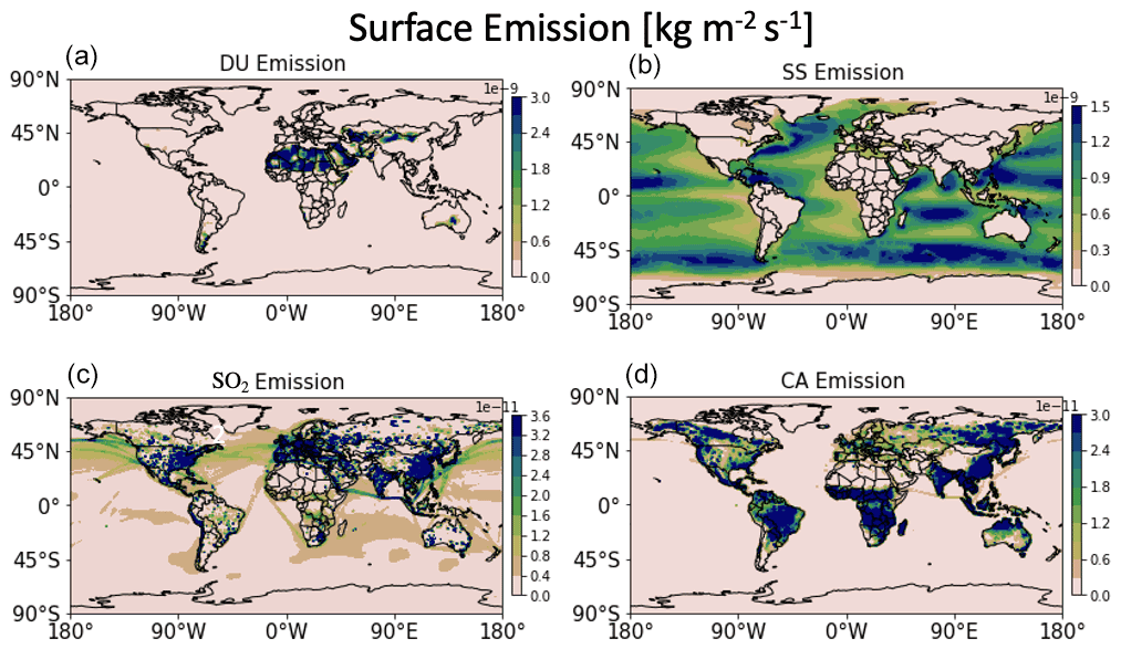
Figure 2Annual surface emission (kg m−2 s−1) of (a) DU, (b) SS, (c) SO2, and (d) CA (BC plus OC) aerosol species during 1997–2014 from MERRA-2 data.
For this study, we use the MERRA-2 aerosol reanalysis (GMAO, 2015a) that has a horizontal resolution of and a temporal resolution of 1 h (Randles et al., 2017). In particular, most of the analysis is based on the zonal and meridional components of the vertically integrated aerosol mass flux data. The MERRA-2 aerosol reanalysis data capture the global aerosol optical depth reasonably well and are validated against 793 Aerosol Robotic Network (AERONET) stations' aerosol measurements (Gueymard and Yang, 2020). For example, we have used the variables dust mass flux in the zonal (DUFLUXU) and meridional (DUFLUXV) directions to compute integrated aerosol transport (IAT) values for dust at each grid. MERRA-2 aerosol data have previously been used in studies investigating aerosol microphysical effect and global aerosol transport (Xu et al., 2020; Sitnov et al., 2020; Chakraborty et al., 2021a). Our previous study using MERRA-2 data successfully detected AARs over various regions of the globe, and the AERONET stations located either in the receptor regions or along the path of AARs have shown a substantial increase in the aerosol optical thickness during AAR events (Chakraborty et al., 2021a).
To examine the vertical profiles of aerosol amount and wind and aerosol mass fluxes (i.e., Fig. 4), we use MERRA-2 3 h instantaneous aerosol mixing ratio data (inst3_3d_aer_Nv) that provide aerosol mass mixing ratio at 72 vertical levels. To assess the information about the zonal and meridional wind, we use MERRA-2's associated meteorological fields (inst3_3d_asm_Nv) with the same resolution as the aerosol mass mixing ratio data (Randles et al., 2017). In addition, we also use MERRA-2 time-averaged, single-level assimilated aerosol diagnostics (GMAO, 2015b) datasets (MERRA-2 tavgU_2d_adg_Nx) to describe the spatial distribution of the emissions of aerosol particles at the surface to examine the relationship between source regions and frequency of occurrence of AARs. MERRA-2 accounts various sources for emissions (Randles et al., 2017). Dust emissions in MERRA-2 use a map of potential dust source locations. Emissions of both DU and SS are wind driven for each size bin and parameterized. Sea salt emission is estimated using the sea surface temperature and the wind speed dependency, with sea salt emission parameterization depending on the friction velocity. For SS, lake emissions are also considered. SU aerosol emissions derive from both natural and anthropogenic sources. Inventories for sulfate include volcanic sulfur dioxide (SO2) emissions and those from the aircraft, energy sectors, and anthropogenic aerosol sources. Emissions of CA and SU aerosols in MERRA-2 come from various inventories over the time. From 2010, the Quick Fire Emissions Dataset (QFED) version 2.4-r6 is used. Locations of fires are obtained from Moderate Resolution Imaging Spectroradiometer (MODIS) level 2 fire and geolocation products. (Please see Table 1 of Randles et al., 2017 for details.) Before that, MERRA-2 utilizes the Global Fire Emission Dataset (GFED) from MODIS. MERRA-2 also applies biome-dependent correction factors and fractional contributions of emissions from different forests, applying corrections to the monthly mean emissions that cover 1980–1996 which are based on Advanced Very High Resolution Radiometer (AVHRR), the Along Track Scanning Radiometer (ATSR), and the Total Ozone Mapping Spectrometer (TOMS) aerosol index.
The AR detection algorithm designed by Guan and Waliser (2015) was to detect and study ARs based on a combination of criteria related to the intensity, direction, and geometry of vertically integrated water vapor transport (IVT). The algorithm and associated AR detection databases (based on multiple reanalysis products) have been widely used by the AR research community (Chapman et al., 2019; Dhana Laskhmi and Satyanarayana, 2020; Edwards et al., 2020; Gibson et al., 2020; Guan et al., 2020; Guan and Waliser, 2019; Huning et al., 2019; Jennrich et al., 2020; Nash and Carvalho, 2020; Sharma and Déry, 2020; Z. Wang et al., 2020; Zhou and Kim, 2019). Details about the AAR algorithm and the modifications made to the AR algorithm to make it applicable for AARs are provided below.
In the initial AAR algorithm (Chakraborty et al., 2021a), we detect AARs daily at four time steps (00:00, 06:00, 12:00, and 18:00 UTC) for a period of 18 years during 1997–2014 and separately for each aerosol species. To compute total IAT over each grid cell at each time step for any species (n) of aerosols, we calculate the following:
where IATU and IATV denote the vertically integrated aerosol mass flux in the zonal and meridional directions, respectively. We are interested in identifying extreme transport events; thus, we first compute the 85th percentile of the IAT magnitude over each grid cell during 1997–2014. Grid cells with an IAT magnitude of less than the 85th percentile threshold are discarded. The remaining grid cells serve as input to the following five steps to (1) isolate the objects (i.e., contiguous areas) of enhanced IAT with values above the 85th percentile, (2) check the consistency of the IAT directions at each grid cell within an IAT object to retain only those objects where at least 50 % of the grid cells have IAT directions within 45∘ of the direction of the mean IAT of the entire object, (3) retain the stronger 50 % of those objects detected in the previous step based on the object mean IAT, (4) retain objectives only if the direction of the object mean IAT is within 45∘ of the along-river axis to ensure that the direction of the aerosol transport is aligned with the river, and (5) apply length and length-to-width ratio criteria and retain only those objects longer than 2000 km with an aspect ratio greater than 2. At the end of these steps, the objects that remain are referred to as AARs and are further characterized in this study. We also show the sensitivity of the detection of AARs to key threshold values used in the above steps in Fig. 9.
In developing the AAR detection algorithm (Chakraborty et al., 2021a), only three changes were made to the original AR detection algorithm. In step 1 of the AR moisture algorithm, a fixed lower limit of IVT, specifically 100 kg m−1 s−1, is applied globally to facilitate the detection of ARs in polar regions, where IVT is extremely weak climatologically due to the very cold, dry atmosphere. We found that this additional filter is not needed for AAR detection. In addition, given the strong meridional moisture gradient between the tropics and extratropics, ARs are primarily recognized as the dominant means to transport water vapor poleward (Zhu and Newell, 1998). Accordingly, the AR algorithm is designed to detect IVT objects with notable transport in the poleward direction. However, since there is no similar and dominant planetary gradient in aerosol concentration in the north–south direction, we removed this constraint on meridional IAT for AARs and instead applied a constraint on the total IAT (i.e., zonal and meridional components combined). Finally, Chakraborty et al. (2021a) computed the climatological 85th percentile threshold IAT values for each month based on the 5 months centered on that month, as in the original AR algorithm (Guan and Waliser, 2015). However, it was found that a 3-month window better resolves the annual cycle of IAT and, meanwhile, still retains sufficient sampling over the period of 1997–2014. For example, the IAT 85th percentile for February is calculated using the IAT values 4 times each day during January–March of 1997–2014.
AAR frequency at each grid cell is calculated as a percent of the time steps that AARs are detected at that grid cell and expressed in units of days per year for annual means (by multiplying the percentage by 365 d yr−1) and days per season for seasonal means (by multiplying the percentage by 91 d per season). The mean zonal and meridional IAT associated with AARs over each grid cell at latitude φ and longitude λ are calculated as follows:
where N is the number of times AARs were detected over that grid cell.
To obtain the fraction of total (i.e., regardless of AAR or non-AAR) annual transport conducted by AARs of five different aerosol species, we first temporally integrate IATU and IATV over all the time steps when AARs were detected over a grid cell at latitude φ and longitude λ, as follows:
where dt is the duration between each time step (6 h), and T is the total duration for 18 years. Based on that, the magnitude of annual AAR IAT, which is a scalar quantity, at each grid cell is calculated as follows:
Similarly, we compute Total_all_annual_IATφ,λ for all the time steps (i.e., AAR and non-AAR combined). Next, since the annual AAR IAT and annual total IAT are not expected to be in exactly the same direction, we project the former onto the latter. For that, the directions of the two vectors are obtained as follows:
Finally, the fraction of total annual transport conducted by AARs is obtained as follows:
where .
4.1 Overall aerosol transport and surface emission
To provide a background for characterizing the seasonality of AARs, we first illustrate the seasonal variability in the overall aerosol transport (i.e., regardless of AAR conditions) during 1997–2014 (Fig. 1). Here, we combine black carbon (BC) and organic carbon (OC) aerosols, denoted as CA, owing to their similar sources and seasonality (BC and OC are accounted for separately in subsequent analysis of AARs). Dust IAT (first column; Fig. 1) is higher during the MAM and JJA seasons. Global deserts, such as the Sahara, Gobi, and Taklamakan deserts, and the Middle East act as a significant source of dust aerosols year round (Fig. 2a), emitting more than kg m−2 s−1 of dust, primarily in the northern spring. The sea salt IAT (second column; Fig. 1) increases during the winter seasons of the Northern and Southern hemispheres due to the increased mean westerly flow and storm activities during these seasons. Annual maps of SS emission (Fig. 2b) show that a large number of SS aerosols are emitted over the global oceans, especially over the tropical oceans because of the convective activities, and in the midlatitudes where synoptic storm activities are dominant. Sulfate IAT (SU; third column; Fig. 1) is high over a region between China and the North Pacific Ocean region, extending up to the western USA, during all seasons with the lowest SU IAT values in JJA. The large SU IAT values (Fig. 2c) are likely due to high emissions of SO2 over China (Dai et al., 2019; Wang et al., 2013) coupled with strongly varying synoptic flows. A secondary region of a higher amount of SU IAT is also detected between the eastern USA and the northwestern Atlantic Ocean, as a high amount of SO2 is emitted east of the Rocky Mountains, particularly over the Ohio valley (Fig. 2c). Figure 2c also shows that some SO2 is emitted due to global shipping activities.
Globally, boreal and rainforests are the most significant contributors to the CA aerosols (Fig. 2d). Accordingly, it appears that the Congo rainforest dominates the Amazon rainforest in terms of CA IAT (right column; Fig. 1). The Amazon rainforest region has higher IAT during its dry and transition seasons and lower IAT in the wet season. Similarly, the Congo rainforest releases a high amount of CA aerosols during the dry season (JJA) and another peak in the Sahel during DJF (Fig. 2d). An increase in dry period CA IAT might be due to the increased vegetative stress, forest fire, and agricultural burning over these two regions. However, it is interesting to note that the Congo rainforest also emits CA aerosols during the boreal autumn (SON) rainy season, which is the stronger of the two rainfall seasons in this region, but not during the MAM rainy season. In MAM, the tropical rainforests over eastern India, Myanmar, and southern China have higher CA IAT values. Emissions from the boreal forests appear to be less than that of the rainforests. Over most of the midlatitudes in the Northern Hemisphere, the emissions of CA aerosols (Fig. 2d; also IAT values in Fig. 1d) are less than that over the global rainforests and China in all four seasons (Fig. 1). As a result, although CA (OC and BC) AARs are more frequent over the midlatitude region, and the mean IAT by those rivers is less than those AARs that originate from the global rainforests and China (Chakraborty et al., 2021a). These results point out the existence of seasonality and variability in the overall aerosol emission and transport. As a result, we expect the frequency and intensity of AARs might also vary among different seasons in accordance with the distribution of surface emissions.
4.2 AAR frequency and intensity
To illustrate the characteristics of individual AAR objects, Fig. 3 shows examples of AARs of each species, including the location, shape, and transport direction and magnitude. Also indicated in the figure is the length and width of each illustrated AAR. Figure 3a shows all the DU AARs detected on 25 June 2008 at 12:00 UTC. Many of those DU AARs are detected between the Sahara desert and the Caribbean, the Middle East region and Europe, over the central USA, and over the Patagonia region. Figure 3d shows details of one DU AAR (encircled in Fig. 3a) that extends from the western boundary of the Sahara desert to the southern USA and Caribbean and has IAT values greater than kg m−1 s−1. The AAR is 8082 km long and 1158 km wide. Similarly, we show details of one SS AAR (Fig. 3e) with a length of 5295 km and a width of 984 km (IAT kg m−1 s−1) over the Southern Ocean among other AARs detected on 19 January 2010 at 12:00 UTC (Fig. 2b). Unlike DU AARs, SS AARs are located mostly over the ocean (see also Fig. 4) and carry the extratropical AR signature. SS AARs over the tropical regions appear to be smaller than the extratropical AARs in Fig. 3b.
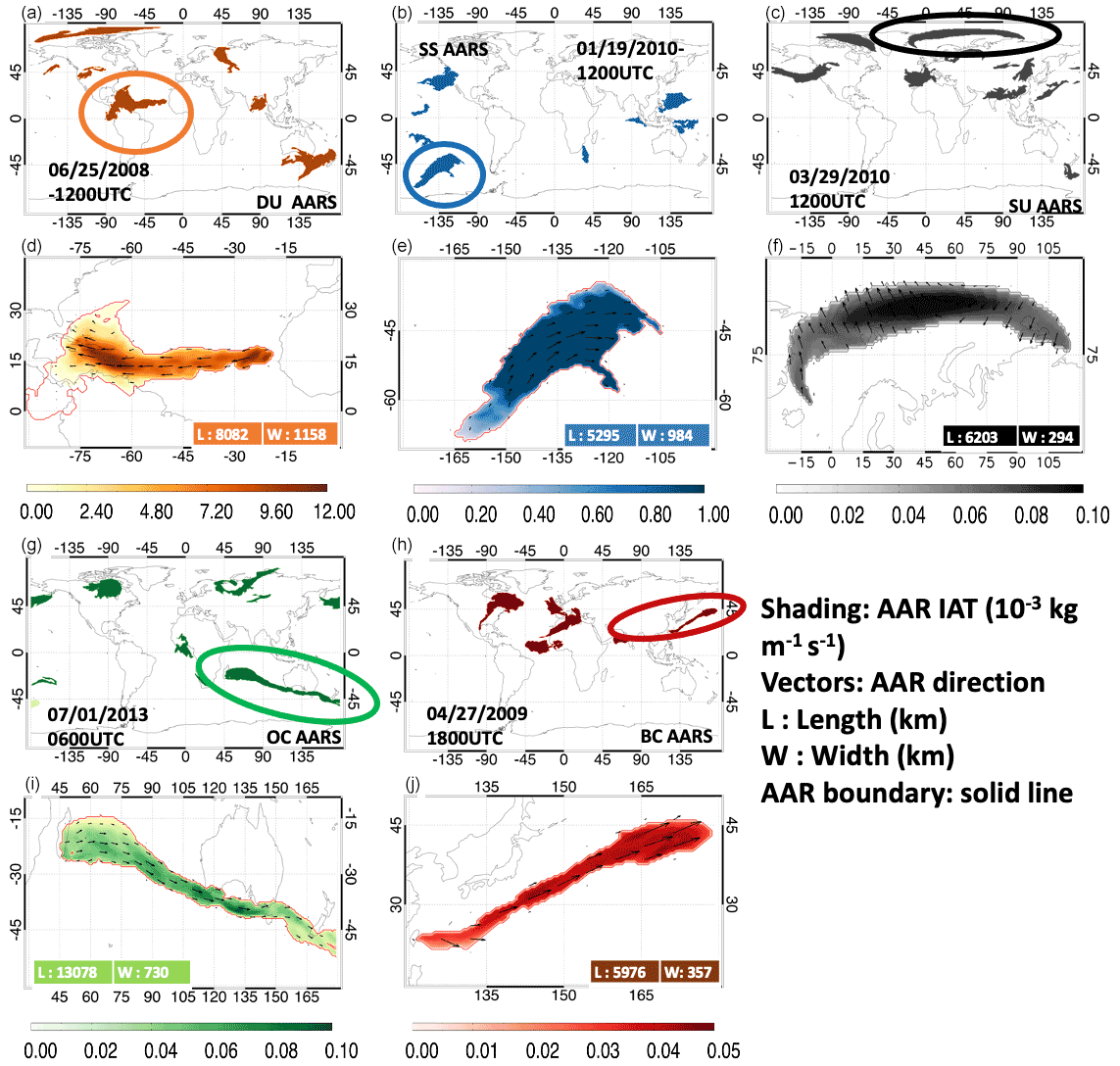
Figure 3Detection of five different species of aerosols atmospheric rivers. Panels (a)–(c), (g), and (h) show all AARs detected for a given species at an arbitrary time step (see the bottom of each panel for the aerosol species and time stamp). Panels (d)–(f), (i), and (j) show the detail (encircled; see the legend) of a specific AAR from the corresponding panel above.
A number of SU AARs occurred in the polar region due to the Eyjafjallajökull volcanic eruption (Fig. 3c). The volcano, located in Iceland, erupted on 20 March 2010, causing disruption to the aviation industry (https://volcanoes.usgs.gov/volcanic_ash/ash_clouds_air_routes_eyjafjallajokull.html, last access: 1 January 2022). In Fig. 3f, we show details of one of these SU AARs on 29 March 2010. The SU AAR is 6203 km long and 294 km wide and transported a large amount of SU aerosols (IAT kg m−1 s−1) into and across the polar region. It is important to notice that MERRA-2 did not include the ash aerosols that were co-emitted with the SO2 plumes that were eventually converted into sulfate aerosols by gaseous and aqueous processes. In April 2010, our algorithm detected ∼80 SU AARs (at every 6 h of interval, i.e., 20 SU AAR days) originating over that region and propagating to different directions.
Hereinafter, we separately show the CA rivers as OC and BC rivers, especially because BC AARs can significantly impact the radiative forcing compared to OC AARs and because the mean mass of aerosols being transported by the OC is about 5 times that of BC AARs (Fig. 4). Figure 3g shows examples of OC AARs detected on 1 July 2013. We show details of one OC AAR that stretches from Madagascar to New Zealand in Fig. 3i. The OC AAR is 13078 km long and 730 km wide and flows west over the Indian Ocean with an IAT of kg m−1 s−1. Figure 3h shows a few BC AARs detected on 27 April 2009. BC AARs often originate near the China–northwestern Pacific Ocean region (see also Fig. 4). We show the details of one such BC AAR in Fig. 3j. It is to be noted that the IAT values of BC AARs are smaller than the OC AARs; however, they might play a significant role in the atmospheric radiation budget owing to the capability of BC aerosols to absorb solar energy.
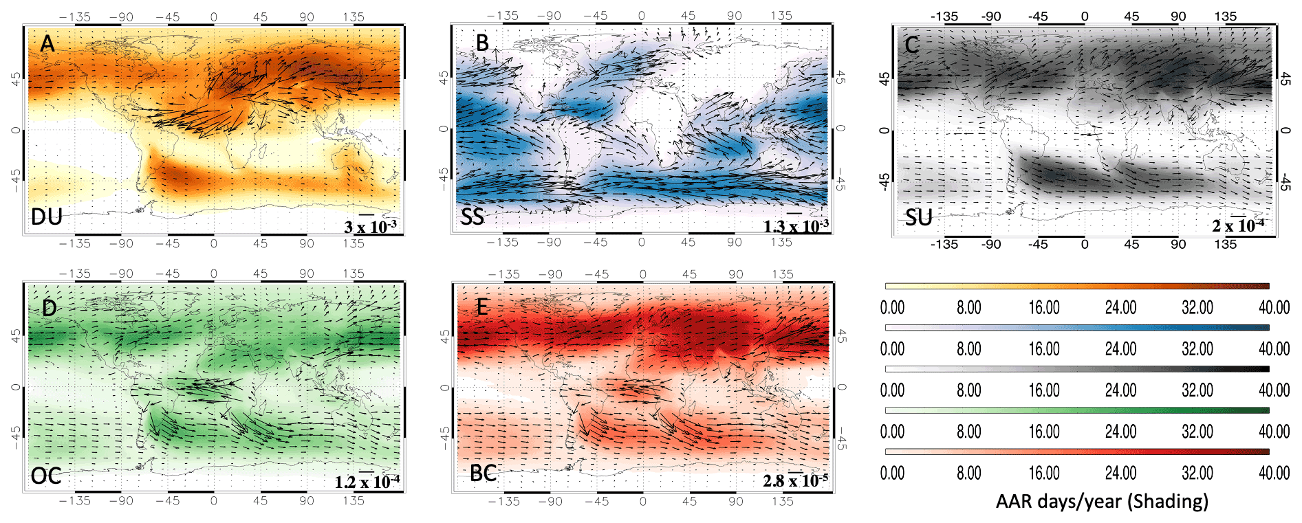
Figure 4Annual climatological AAR frequency (days per year; shading) and IAT (arrows; kg m−1 s−1) during 1997–2014 based on MERRA-2. (a) Dust. (b) Sea salt. (c) Sulfate. (d) Organic carbon. (e) Black carbon. Scales for the IAT vectors are provided in the lower right side of each plot.
To illustrate the overall climatology of AARs, Fig. 4 shows the annual mean frequency of occurrence (shading; days per year) and the mean IAT (arrows; kg m−1 s−1) associated with AARs. Figure 4a shows that a strong anticyclonic motion over the Sahara desert is associated with many DU AARs, consistent with the annual DU emission (Fig. 2a) and seasonal DU IAT (Fig. 1 – leftmost column) over that region. Around 30 AAR d yr−1 (shades) carry on average 3–15 kg m−1 s−1 (vectors) of dust from the Sahara desert over the North Atlantic Ocean and reach the southern USA and the Caribbean regions. A similar number of AARs also transport aerosols towards Europe and the middle east region. A relatively high number of DU AARs are detected over China, Mongolia, and Kazakhstan; however, the mean transport over these regions by AARs is lower (IAT kg m−1 s−1) than those originating from the Sahara desert. The southern hemispheric deserts also emit numerous AARs but with a smaller amount of dust transport as the dust emissions (Fig. 2a) and IAT (Fig. 1) are low over there. Overall, the Sahara desert dominates any other desert in the world regarding the formation of the strongest and most intense DU AARs.
Figure 4b shows the climatological maps of SS AARs. SS AARs are mostly located over the global oceans, especially over the tropical and subtropical trade wind regions. The SS AARs in the midlatitudes carry the signature of the storm tracks and have distributions similar to ARs (Guan and Waliser, 2015). Every year, in the midlatitude region, 30–40 ARs are detected (Chakraborty et al., 2021a), whereas ∼20 AAR d yr−1 occur in the midlatitudes with mean a IAT of kg m−1 s−1. The distributions between ARs and SS AARs are not quite the same; the SS AARs are biased equatorward toward the trade winds. In comparison, tropical SS AARs are more frequent but have less IAT than the midlatitude SS AARs. Around 30 SS AARs have mean IAT of kg m−1 s−1 over the tropical region.
It is important to note SU AARs are more frequent (∼40 d yr−1; Fig. 4c) in the Northern Hemisphere than in the Southern Hemisphere, consistent with the predominance of emissions of SO2 over China, Europe, and the eastern USA (Fig. 2c), owing to anthropogenic emissions and biogenic activities in these regions. It is important to note that MERRA-2 aerosols data do not account for biogenic sources like carbonyl sulfide in the version of the data we have used for this study. The SU AAR hotspot regions over the Southern Hemisphere include pathways from the southern edges of the global rainforests to the south Indian, south Atlantic, and Southern Oceans. Mean IAT ( kg m−1 s−1) by SU AARs is lower than that of the DU and SS AARs. Many BC and OC AARs originate from the global rainforests, such as the Congo and Amazon, and from the regions that are susceptible to biomass burning and CA aerosol emissions, such as Europe, the eastern USA, industrialized areas over eastern China, and northern India. Annually, 20–40 BC or OC AARs are generated from these regions. It appears that BC AARs are more numerous than the OC AARs; however, OC AARs have larger IAT than BC AARs.
4.3 Vertical profiles of AAR aerosol mass flux and wind
To understand the anomalous atmospheric conditions that account for an AAR event, it is important to know the relative contribution of the two quantities that make up these IAT extremes, namely the aerosol mixing ratio and the wind speed. Also, as mentioned before, the altitude of aerosol particles within AARs can be of importance due to aerosol impacts on the radiation budget, convective anvil lifetime (Bister and Kulmala, 2011), cloud formation (Froyd et al., 2009; Khain et al., 2008), and air quality near the surface. Here, we characterize the vertical profiles of the AARs at a number of different locations with high AAR frequency (see the inset map in the middle column; based on Fig. 4). For example, the orange box over the Saharan–Caribbean pathway experiences a presence of 25–30 AARs yr−1 (Fig. 4a). Based on our analysis between 1997 and 2014, the profiles in Fig. 5a, b, and c show the mean and standard deviation of ∼ 400–500 AARs.
It is important to keep in mind that the aerosol vertical structure in MERRA-2 is not directly constrained by measurements and is chiefly determined by the injection height of the emissions and turbulent and convective transport processes parameterized in the model. Evaluation of the vertical structure of MERRA-2 aerosols appears in Buchard et al. (2017). Buchard et al. (2017) has used Cloud-Aerosol Lidar and Infrared Pathfinder Satellite Observation (CALIPSO) to examine the vertical structure of aerosols in MERRA-2. The left column of Fig. 5 shows the composite vertical profiles of aerosol mass fluxes for each aerosol species; both those for AARs (solid) and for all time steps regardless of AAR conditions (dotted) are shown for comparison. Mean fluxes of the synoptic AAR events are larger than the overall annual mean over all the regions, which is not unexpected since AARs represent the extreme transport events. For DU AARs (Fig. 5a), the strongest transport is observed between the Sahara desert and North Atlantic/Caribbean (orange) and western Europe/Middle East (red) pathways. Flux values decrease with altitude within AARs that transport aerosols from the Sahara desert to the Europe/Middle East region (red). However, AARs that transport aerosols from the Sahara desert to the North Atlantic region (orange) have peak IAT values near 750 hPa. There is also a secondary peak at the 960 hPa height (Fig. 5a). The aerosol mixing ratio (Fig. 5b) slightly decreases from the surface up to a height of 960 hPa and then increases above it. This might suggest the influence of the gravitational force and settlement on the aerosol mixing ratio, as observed in many of the aerosol mixing ratio profiles of other species over other regions (for example, the red line showing the aerosol mixing ratio profile for the Sahara to European pathway). However, a smaller peak in the wind profile (Fig. 5c) around 950 hPa indicates the influences from the low-level jets and the seasonal variations in the transatlantic dust transport that have not been studied yet. A detailed seasonal analysis is required to understand the existence of the smaller peak at 960 hPa. However, the presence of the African easterly jet–north (AEJ-N) above, centering at 600–700 hPa, further lifts the aerosols and attains a peak around 750 hPa.
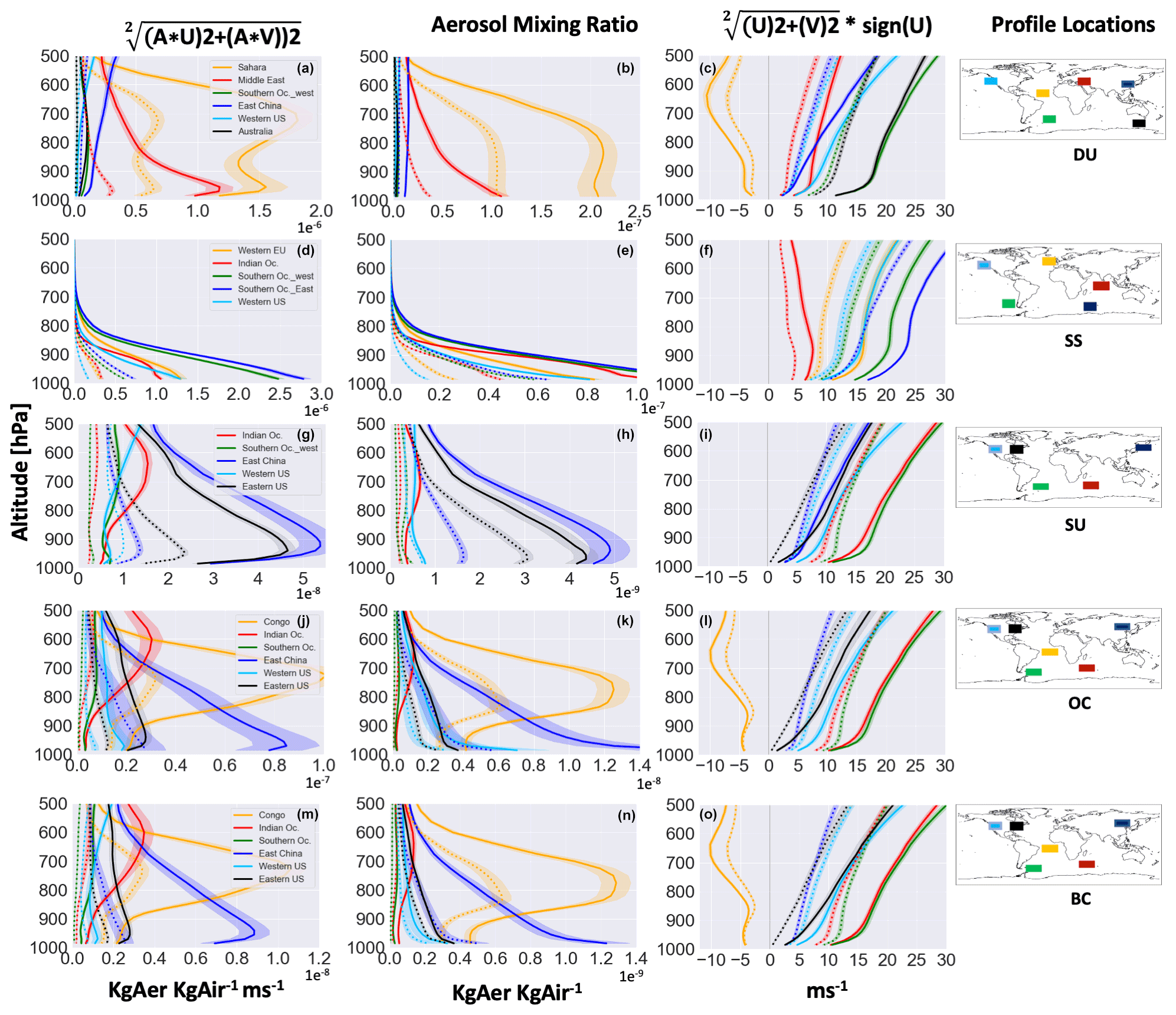
Figure 5Average vertical profiles of (a, d, g, j, m) aerosol mass fluxes, (b, e, h, k, n) aerosol mixing ratios, and (c, f, i, l, o) wind speed over a number of locations for AAR events (solid) and all (dotted) time steps. Please see the AAR frequency maps in the inset of the middle panel for the locations chosen to calculate the profiles. In panels (c, f, i, l, o), a sign convention (see the column title) is used to highlight the general east–west direction of the wind speed profiles.
We also show the vertical aerosol mixing ratio profiles (middle column) and the wind profiles (right column) separately to help disentangle their influences on the aerosol flux profiles. Given the very few globally gridded datasets to use for this purpose, we have relied on the data provided in the MERRA-2 data, which in this case is provided as aerosol mixing ratio. Figure 5b shows that high aerosol levels inside AARs over the Sahara desert to Caribbean pathway extend vertically up to the 700 hPa height, with a peak around 750 hPa, unlike any other regions analyzed. The third column, which shows the mean wind speed profile multiplied by the sign of the zonal wind to show the east–west direction of the AARs, confirms the influence from the AEJ-N (Cook, 1999; Wu et al., 2009) on the AARs wind profile that peaks around 650 hPa and lifts aerosols over this region (Fig. 4c). Higher flux values near the surface are due to a high aerosol mixing ratio, but as altitude increases, higher flux values inside AARs are contributed by both the aerosol lifting and the high zonal wind speed of AEJ-N between the Sahara desert and the North Atlantic Ocean region. Other regions like the Southern Ocean (near South America), Australia, eastern China, and western USA have a smaller aerosol mixing ratio as compared to the Sahara to the North Atlantic Ocean and Caribbean and Sahara to Europe/Middle East pathways. Wind speed contributes to larger flux values as altitude increases over some of these locations near eastern China, the Southern Ocean, Australia, and the western USA; however, their flux values are smaller than those taking off the Sahara desert.
Aerosol flux and mass mixing ratio profiles for SS species (Fig. 5d and e) decrease with altitude. This is because the SS particles are typically found within the boundary layer (Gross and Baklanov, 2007), are larger in size, and often form due to high wind speed and surface evaporation along the storm tracks and may not travel long distances outside the storm tracks (Sofiev et al., 2011; May et al., 2016). The largest aerosol mixing ratio and IAT values are observed over the Southern Ocean consistent with the persistent and year-round AAR activities over there.
Consistent with the SO2 emission (Fig. 2c), eastern China (blue line) dominates in terms of SU aerosol mass mixing ratio by a factor of 5 as compared to the other regions (Fig. 5h) analyzed and shown here. The aerosol mixing ratio (Fig. 5h) and the flux values (Fig. 5g) increase with height, attaining a peak around 900 hPa over there, and probably exhibit the impact of the boundary layer inversion effect on the accumulation of the pollutants (Li et al., 2017). Above 900 hPa, both the aerosol mass mixing ratio and flux values gradually decrease. However, the SU aerosol mass mixing ratio decreases when those AARs reach the western USA five times (Fig. 5h). Owing to the fact that the eastern USA originates many SU AARs that can contribute to a transatlantic transport driven by strong westerly winds, we have also computed the IAT profiles of SU AARs generated over there. Figure 5g and h show that AARs over the eastern USA also have a high IAT (Fig. 5g) and aerosol mass mixing ratio (Fig. 5h). Flux profiles and aerosols mixing ratio over the Indian Ocean (red) and Southern Ocean (green) show different behavior. Aerosols appear to be continental in origin and are lifted to attain a peak concentration around 650 hPa. Contributions from wind speed (Fig. 5i) as compared to aerosol mixing ratio (Fig. 5h) appear to be less on the SU flux profiles (Fig. 5g) since the wind speed associated with AARs is the highest over the Indian and Southern oceans, but the largest flux values are associated with the AARs over the eastern China region which has the largest aerosol mass mixing ratio.
Next, we examine the vertical profiles of CA AARs over the Congo Basin, the western USA, eastern China, the Indian Ocean, and the Southern Ocean. As in the case of dust aerosols over the Sahara desert to North Atlantic transport pathway (Fig. 5a; orange line), both the OC and BC AARs off the Congo Basin show elevated flux values around 700 hPa (Fig. 5j and m). It is to be noted that the wind speed within AARs peaks around 650 hPa, suggesting the influence from the AEJ-S (south; Adebiyi and Zuidema, 2016; Chakraborty et al., 2021b; Das et al., 2017) on the AARs' wind profile (Fig. 7k and n) that might be responsible for the peaks in the aerosol mixing ratio profiles around 750 hPa (Fig. 5l and o) instead of the exponential profiles as observed in most of other regions. AARs over eastern China (blue) also carry a large number of near-surface aerosol particles that contribute to large BC and OC IAT values in this region. However, when those AARs reach the western USA, the number of the BC and OC aerosol mass mixing ratio significantly decreases by ∼8 times, presumably because of the settlement and removal of the aerosol particles during the transport. As compared to SU AARs, the IAT values and aerosol mass mixing ratio of OC and BC AARs over the eastern USA is significantly lower (3–4 times less) than those originating from China and the Congo rainforest. Wind speed appears to have less influence on the flux profiles since the Indian Ocean and the Southern Ocean have the largest (smallest) wind speed (flux values) associated with the AARs.
4.4 Fraction of total annual transport accounted for by AARs
It is apparent from Fig. 5 that the mean IAT averaged over AAR time steps is greater than the mean IAT averaged from all time steps. This is not surprising, since AARs detected by our algorithm represent the extreme transport events (see Sect. 2 for the definition and methodology). Considering that the original analysis on water vapor ARs (Zhu and Newell, 1998) highlighted that 90 % of the poleward transport of water vapor in the midlatitudes occurred in a relatively small number of extreme transport events (i.e., ARs), a similar question can be raised here for AARs. Specifically, what fraction of the total annual aerosol transport is accounted for by the 20–40 AAR days that occur each year on average (Fig. 4)? Also, do AARs transport a higher fraction of the total global annual transport over the major aerosol transport pathways, and is this dependent on aerosol species? In Fig. 6, we show the fraction of total annual IAT accounted for by AARs (shades), counting only the component of AAR transport in the direction of the total annual transport (arrows). Figure 6a shows that, annually, ∼ 40 000–100 000 kg m−1 of DU IAT is transported by All events (i.e., considering all data points in the record) that originate from the Sahara desert. Near the Equator, the fractional transport by AARs (FAAR) is around ∼20 % over the Atlantic Ocean in the direction of the Amazon rainforest (Fig. 6a), which is realized within ∼30 AAR d yr−1 (see Fig. 4a). In this same longitude sector, FAAR gradually increases with latitude and reaches up to 80 % around 35–40∘ N, where AARs act to transport dust from the Sahara desert to Europe and the Middle East region. Over Mongolia and China, the total annual IAT is ∼ 20 000–40 000 kg m−1 and about 30–40 AAR d yr−1 (Fig. 4a) contribute up to ∼ 40 %–50 % of that transport. In the Southern Hemisphere, Patagonia and South American drylands give rise to ∼4000 kg m−1 of annual dust transport and AARs contribute to a maximum of 20 %–40 % of that transport in about 20–30 AAR events per year (Fig. 4a). Over some regions far from the dust source region, such as over the maritime continent, the annual IAT value is very small by all events (Fig. 6a). About 5 AARs (shading, Fig. 4a) with very small object mean IAT values (arrows, Fig. 4a) are observed over there each year. It appears that, although AARs are not frequent (∼5 AAR d yr−1) over there, they are responsible for 80 %–100 % of the total annual transport.
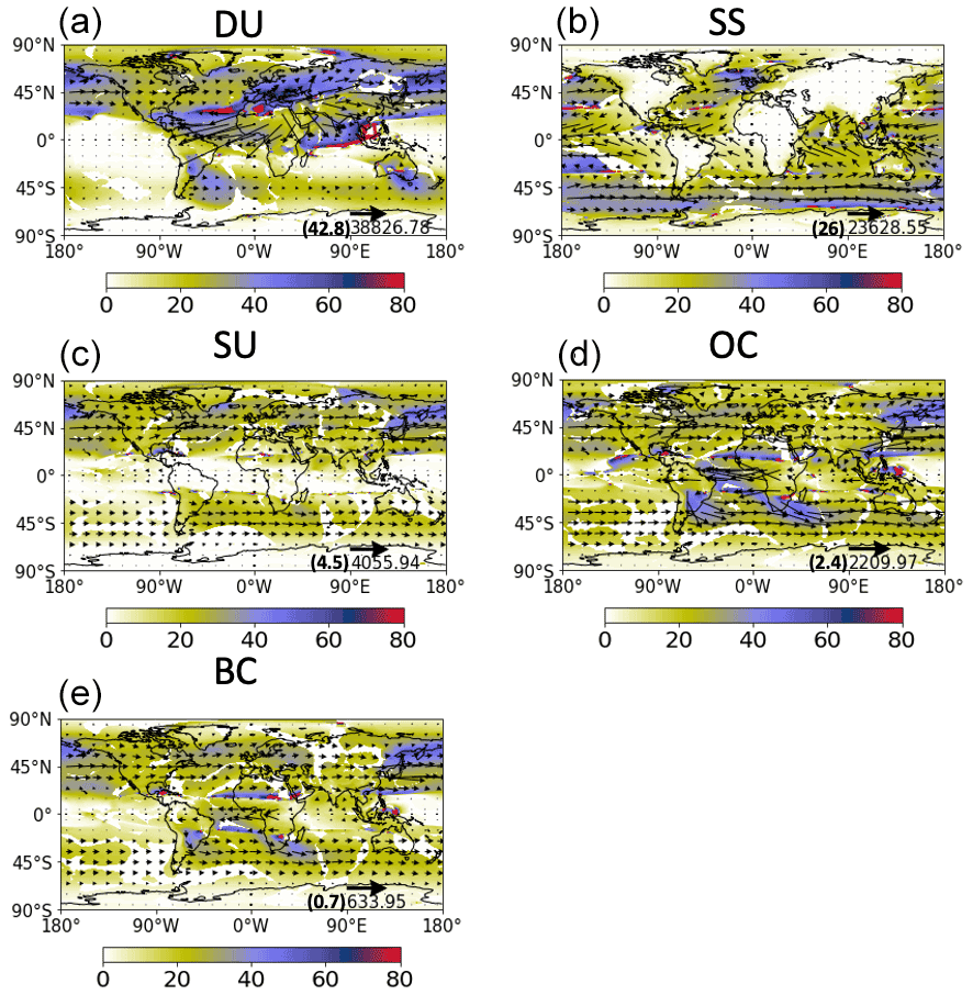
Figure 6Fraction of annual total IAT transport (arrows; tonnes are shown in parentheses, followed by kg m−1) accounted for by AARs (%; shading) of five different aerosol species.
SS AARs are far more frequent over the oceans than over the land (Fig. 4b), with peak frequencies of about 30 AAR d yr−1 occurring over the subtropical trade wind regions, the Southern Ocean and northern Atlantic Ocean. In these regions, the total annual IAT is about 10 000–20 000 kg m−1, and FAAR is about ∼ 20 %–30 % in the subtropical regions, reaching a maximum of ∼50 % over the Southern Ocean and the northern Atlantic Ocean (Fig. 6b).
AARs for other species of aerosols can contribute to a maximum of 40 % of the total annual IAT over their major transport pathways. For example, the ∼30 SU AAR d yr−1 that originate over China (Fig. 4c) transport ∼ 30 %–40 % of the total annual aerosol transport (∼2500 kg m−1) over the northern Pacific Ocean. FAAR associated with OC (BC) AARs reaches a maximum of 40 % (30 %) between the Congo Basin and the tropical Atlantic Ocean. Over China and the North Pacific Ocean, South Africa and the Southern/Indian oceans, south China and the western Pacific Ocean, and Amazon and the southern Atlantic/Southern oceans FAAR can reach up to a maximum of 40 %. Higher FAAR is also observed, despite low total annual IAT, over the northern part of the Sahel region for both BC and OC AARs.
4.5 AAR seasonality
Figure 7 shows AAR frequency along with the direction and magnitude of the mean AAR IAT during four different seasons. DU AARs (shading) originate during all the seasons over the Sahara desert. DU AAR IAT (arrows) is higher during DJF and MAM over the Sahara desert owing to a stronger anticyclonic motion in the boreal winter and spring. The largest number of DU AARs are generated during the MAM season when the DU IAT is the highest (Fig. 1) and widely spread across the Northern Hemisphere. In JJA and SON, DU AARs appear to have lower IAT (shorter arrows) but are more frequent than in the DJF season. The frequency of SS AARs also depends on the season. A higher number of SS AARs is detected over the eastern Pacific Ocean and the west coast of the USA, northern Atlantic Ocean, and Europe in DJF and MAM. In JJA, no SS AARs are detected over there. Over the Southern Ocean, SS AARs with large IAT are more frequent during austral winter or MAM and JJA. In comparison, tropical SS AARs are present year round.
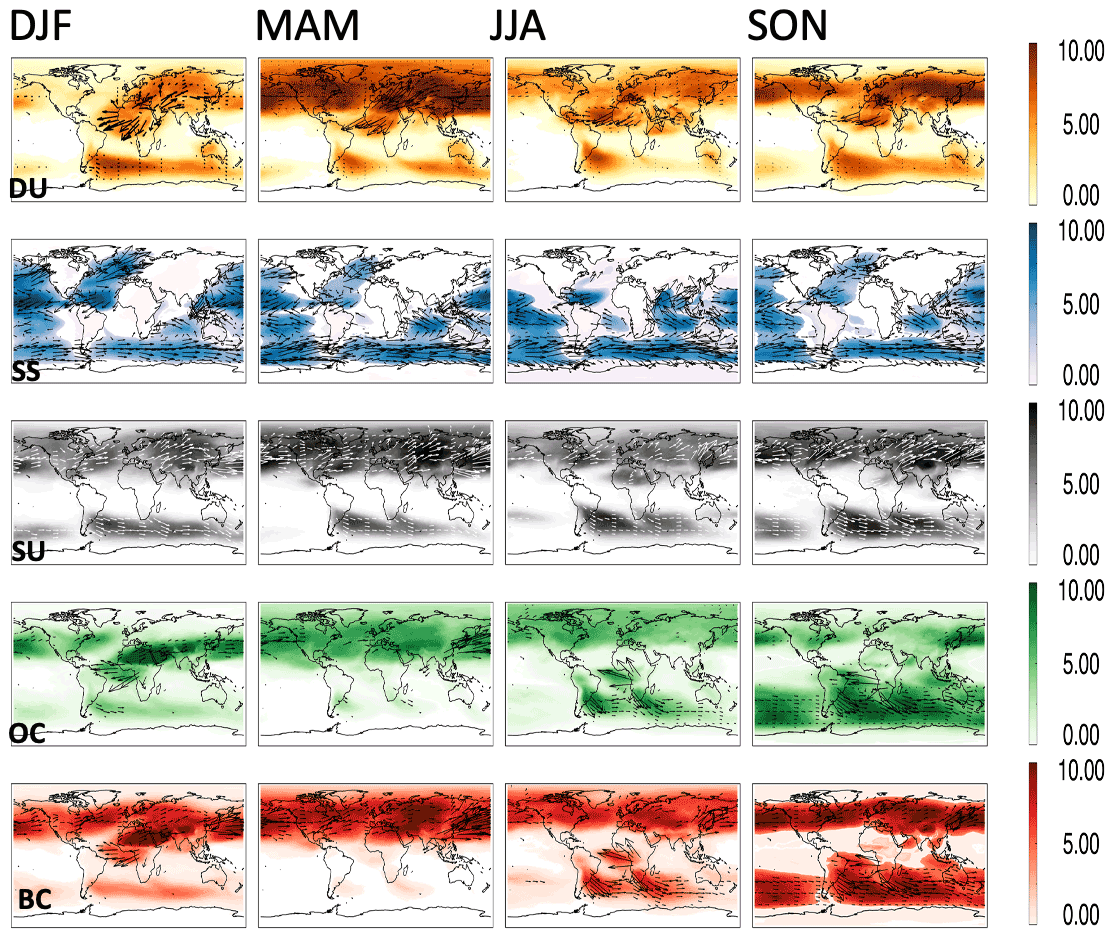
Figure 7Seasonal variations in the AAR frequency (days per season) and IAT (arrows) for five different species of aerosols.
SU AARs in the Northern Hemisphere are more (less) frequent in MAM (JJA) and can be related to the seasonal variations in IAT there (Fig. 1). The frequency of occurrences of SU AARs is higher during SON compared to DJF, while their IAT values are larger in DJF. This might be because of the readiness of sulfate aerosols to form cloud condensation nuclei (CCN) and their hygroscopic nature. The occurrences of intense AR-related precipitation in DJF over the extratropical region in the Northern Hemisphere might cause scavenging and wet removal of SU aerosols when the AARs and ARs coexist. A detailed investigation considering AR-AAR interactions is needed in future studies to better understand the coexistence and influence of AARs and ARs.
Over the Congo rainforest, several OC AARs occur during its dry season (also when CA IAT is high; Fig. 1). A similar frequency of occurrences of OC AARs is also observed during the dry season over the Amazon rainforest. Many OC AARs occur east of China during the DJF and MAM season when the IAT values are large over there (Fig. 1). Many BC and OC AARs are generated over the global rainforests during their dry seasons.
4.6 Basic characteristics of individual AARs and algorithm sensitivities
In this section, we characterize basic features of AARs (Fig. 8), including those related to geometry and IAT intensity and directions, and discuss and show the sensitivity of various AAR features to algorithm specifications and thresholds (Fig. 9). Figure 8a shows that the frequency of AARs decreases monotonically as AAR length increases for all aerosol species. The mean lengths of DU, SS, SU, OC, and BC AARs are 4264, 3722, 4121, 4528, and 4378 km, respectively. Figure 8b shows that AAR widths exhibit a skewed distribution, unlike AAR lengths, implying an optimum or common value for AAR widths around 400 km. The mean width of DU, SS, SU, OC, and BC AARs is 586, 642, 542, 625, and 589 km, respectively. When considered together in the form of the aspect ratio of AARs, i.e., length width ratio, the distribution is also a skewed distribution (Fig. 8c). The lengths are typically 7–8 times their widths due to the skewness of the distribution. DU and SS AARs are the two species having the largest object mean IAT values (Fig. 8d). While, on average, DU AARs have IAT ∼1.65 and kg m−1 s−1, respectively, SU, OC, and BC AARs have smaller IAT (Fig. 8d). Average object mean IAT values for SU, OC, and BC AARs are 0.1, 0.1, and kg m−1 s−1, respectively. The frequency of object mean IAT for BC AARs decreases sharply and seldom reaches beyond kg m−1 s−1. SU (OC) AARs attain a maximum object mean IAT values around kg m−1 s−1, with a maximum frequency of ∼0.6 (0.4).
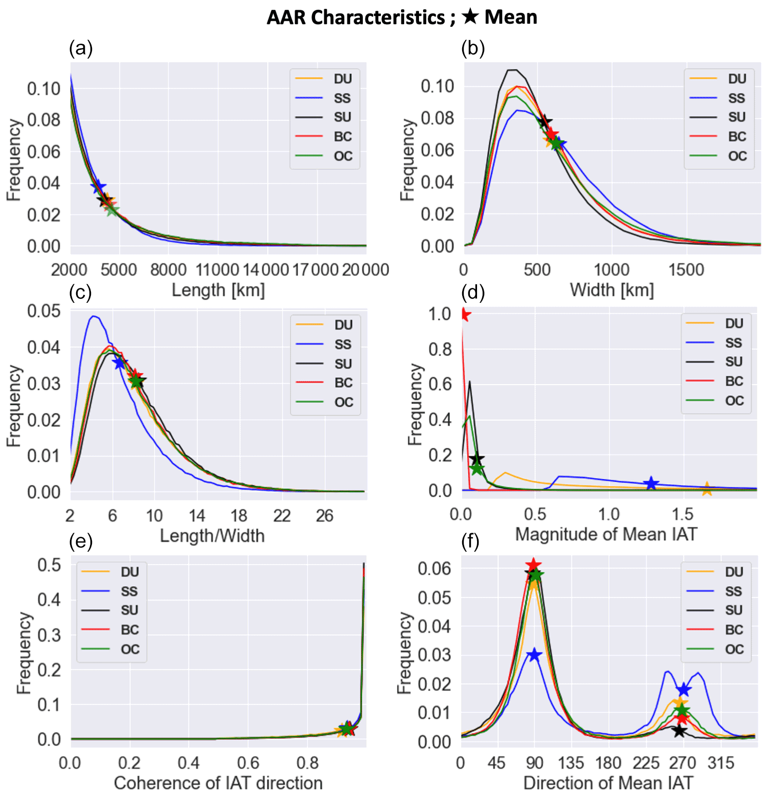
Figure 8Histograms of characteristics of individual AARs. The star (⋆) symbols denote the mean. (a) Length. (b) Width. (c) Aspect ratio. (d) Magnitude of mean IAT. (e) Coherence of the IAT direction. (f) Direction of mean IAT.
The coherence of IAT directions (Fig. 8e) is computed as a fraction of the number of grid cells with IAT directed within 45∘ of the direction of the object mean IAT to all the grid cells within that AAR. A large value implies that a larger fraction of the grid cells has IAT directed in the same overall direction as the AAR. AARs of all the species have a mean coherence of IAT directions between 0.91 (DU) and 0.94 (SU). The distribution of the direction of the object mean IAT implies that the AARs are mostly directed in the zonal direction (Fig. 8f). Relative to north, peak frequencies near 90∘ and between 250 and 310∘ imply that the AARs are either westerly or easterly in nature. A few westerly AARs also transport aerosols in the northeasterly (45–90∘) and southeasterly (90–135∘) directions. A wider peak between 250 and 310∘ implies that most of the easterly AARs also have meridional components in the southwesterly and northwesterly directions. The average values of the object mean IAT direction for all the species of AARs are ∼90∘ (westerly) and between 260 and 270∘ (easterly). These results show that the AARs mostly transport aerosols in the zonal direction as compared to ARs that have notable transport of water vapor in the meridional direction (Guan and Waliser, 2015).
Finally, Fig. 9 shows the sensitivity of AAR detection in our algorithm to three primary thresholds that define the geometry (length and aspect ratio) and grid-wise IAT limits (to identify the extreme transport) of AARs. The results presented above in this study are based on a length limit of 2000 km, aspect ratio limit of 2, and a pixel-wise IAT limit of the 85th percentile. Keeping the length and aspect ratio limits fixed, while increasing the IAT limit to the 90th and 95th percentile values, yields a lower number of AARs detected (top row). On the other hand, relaxing the length limit to 1750 and 1500 km greatly increases the number of AARs detected (middle row). Relaxing the aspect ratio limit to 1.5 and 1 does not significantly alter the number of AARs detected, suggesting that the other limits applied (such as length greater than 2000 km) already effectively remove IAT objects that are not elongated. It appears, from Fig. 9, that grid-wise IAT thresholds pose a large sensitivity to AARs detection as the number of AARs detected is reduced roughly by half as we increase that threshold to the 95th percentile from the 85th percentile used in our main analysis.
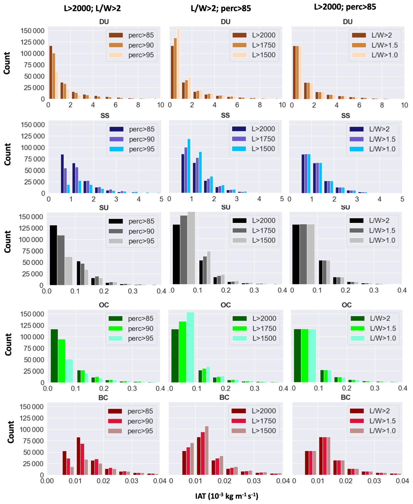
Figure 9Sensitivity of AAR detection to threshold values used for three key parameters (corresponding to the three columns; see the legend for the parameter being tested and the three values chosen for each test parameter) in the detection algorithm for five aerosol species (corresponding to the five rows; see the panel title for the aerosol species). Shown are histograms of mean IAT of individual AARs detected. For example, the left column shows results based on perturbing the IAT percentile threshold (85th, 90th, and 95th percentiles), while keeping the length (2000 km) and aspect ratio (2) thresholds unchanged from the main analysis presented earlier.
Figure 10 shows the sensitivity of the average global area coverage of all AARs to AAR algorithm parameters. Each bar represents the area-weighted global mean AAR frequency or a spatiotemporal measure of the amount of time/space that there is an AAR. Annually, AARs cover 3.42 % of the global area, respectively. Relaxing the length limits to 1750(1500) km increases the number of detections of AARs; thus, the areal coverage of AARs increases to 3.56 % (3.76 %). On the other hand, increasing the pixel-wise IAT limit to 90th and 95th percentile reduces the areal coverage to 2.44 % and 1.13 %, respectively. Relaxing the aspect ratio does not have any impact on AAR's areal coverage. ARs, on the other hand, account for ∼2 % more of the Earth's surface area than AARs (not shown), likely because the filter based on object mean IVT direction in the AR algorithm preferentially filtered out smaller objects compared to the revised filter in the AAR algorithm based on IAT magnitude.
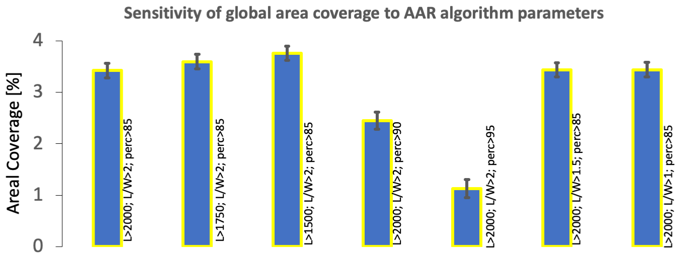
Figure 10AAR and AR sensitivity of the global area coverage to threshold values used for three key parameters in the detection algorithm. For each species of AARs, the first bar shows the average global area coverage for the length limit >2000, aspect ratio >2, and the pixel-wise IAT threshold >85 %. The next two bars show the areal coverage after relaxing the length limit to 1750 and 1500 km. The fourth and the fifth bars show the areal coverage after increasing the pixel-wise IAT limit to 90th and 95th percentile. The last two bars show the areal coverage after relaxing the aspect ratio to 1.5 and 1. Standard deviations show the variations in areal coverage by different species.
Using a newly developed AAR algorithm (Chakraborty et al., 2021a) based on the widely used AR detection algorithm (Guan and Waliser, 2015), we examine a number of important details about AARs that were not explored in Chakraborty et al. (2021a). This includes AAR seasonal variations in frequency and transport values (Fig. 7), the fraction of total annual aerosol transport account for by AARs (Fig. 6), a characterization of their vertical profiles (Fig. 5), relation to the pattern of surface emissions (Fig. 2), along with a number of basic characteristics and distributions for quantities such as AAR length, aspect ratio, object mean IAT, the coherence of the direction of IAT (Fig. 8), and sensitivities of the algorithm to the thresholds chosen for three key parameters (Fig. 9). This study is the first to provide a common detection and analytical basis for studying extreme transport events, heavily leveraging the heritage and methodologies by the (water vapor) atmospheric river community. Moreover, this study identifies the extreme transport events by selecting grid cells with IAT values greater than the 85th percentile of their climatological values and retaining the stronger 50 % of those objects detected based on the object mean IAT values. This study creates a database of the AAR events between 1997 and 2014 that will be expanded till 2020 and will provide a valuable platform for aerosol-transport-related research, including their impacts on the climate and air quality. Furthermore, the algorithm developed to detect AARs can be used to detect the real-time AAR events using the nature run of the GOES FP (forward processing) system that provides analyses and forecasts produced in real time, using the most recent validated GEOS system (https://gmao.gsfc.nasa.gov/GMAO_products/NRT_products.php, last access: 13 June 2022).
The global total annual transport by all and AAR events are inhomogeneous in terms of their geographic distributions. FAAR varies between 0 % and 40 % for SU, OC, and BC AARs, between 0 % and 80 % for DU AARs, and between 0 % and 50 % for SS AARs over various regions of the world. Our results show that, on average, 30–40 SU, BC, and OC AAR days every year are responsible for a maximum of 30 %–40 % of total annual aerosol transport for a given aerosol species over certain major transport pathways around the globe. Over the major transport pathways of the SS (DU) AARs, FAAR can reach up to a maximum of 50(80) % of the total annual aerosol transport of the respective species. The inhomogeneous nature of AARs' spatial distribution and fractional transport out of the annual total suggest a plausible impact of the AARs on the meridional temperature gradient. The attenuation of solar energy by AARs might impact the surface temperature and can thus alter the meridional temperature gradient and the thermal winds. Further analysis will be conducted in the future to delineate the impacts of AARs on the global weather and climate.
The major transport pathways by AARs are also identified in our algorithm for each of the aerosol species. The source of AARs is consistent with the major aerosol emission regions of the world. DU aerosols mostly originate from the global deserts, and their frequency is higher during boreal autumn and spring. SS AARs are mostly located over the global oceans and carry the footprint of the storms. In the midlatitudes, their frequency and intensity increase during the boreal (austral) winter in the Northern (Southern) Hemisphere. Tropical SS AARs are more frequent, but their magnitude of aerosol transport and contribution to the annual aerosol transport is less. A further investigation is needed to understand if/how tropical cyclones and midlatitude storms impact SS AARs differently. CA AARs are generated over the region where biomass burning is more common, like India and China. CA AARs that originate from the global boreal and tropical rainforests have the highest frequency and intensity during their dry seasons but are mostly absent or exist with a reduced frequency during their wet seasons. SU AARs are present year around in the Northern Hemisphere, with a peak frequency and intensity during the dry periods of boreal spring (MAM) and autumn (SON). The frequency of SU AARs occurrences reduces during the boreal summer and winter, presumably due to the summertime convective precipitation events and wintertime synoptic storms. Overall, regions with frequent AAR activities include the Sahara desert to Caribbean and Europe for DU AARs, a circumpolar transport around the midlatitude region in the Northern Hemisphere for all but SS AARs, global oceans and midlatitude storm tracks over the global ocean for SS AARs, global rainforests for BC and OC AARs, and from South America and Africa to the Southern Ocean for DU, BC, OC, and SU AARs.
We have also examined the vertical structure of the aerosol mixing ratio and wind inside AARs. Over most of the major pathways, the aerosol mixing ratio and flux values decrease with height. A higher aerosol mass mixing ratio inside AARs is observed below the 700 hPa over most of the regions and, thus, may have a strong implication on the low cloud cover and surface irradiance. Such an interaction can be complex since shallow clouds also have cooling effects as most of the aerosol species do. Understanding such an interaction between shallow clouds and AARs and their impacts on the cooling effect warrants further investigation. The aerosol mixing ratio (wind speed) appears to contribute a large fraction of IAT below (above) 700 hPa. However, AARs generated from the African continent are the exceptions. Signatures of AEJ-N on DU AARs taking off the Sahara desert and AEJ-S on BC OC AARs originating from the Congo Basin are observed. Both the aerosol mixing ratio and wind speed appear to peak around 600–700 hPa, leading to a higher IAT at the level. The fact that aerosols lift up and attain a peak mass flux around the 700 hPa height for AARs generated from the African continent might have a strong influence on the wet season onset and rainfall mechanisms over there (Chakraborty et al., 2021b). We acknowledge a source of uncertainty in the aerosol mass mixing ratio and IAT profiles shown in this study from the MERRA-2 data, since the MERRA-2 aerosol vertical distribution is also not constrained by satellite-based lidar observations. A recent study found that comparison to the Cloud-Aerosol Lidar and Infrared Pathfinder Satellite Observation vertical feature mask (CALIPSO VFM) data detects a greater occurrence of DU aerosols in MERRA-2 due to errors in the MERRAero aerosol speciation (Nowottnick et al., 2015). In a future study, an in-depth analysis will be performed using the observation from the ground-based and airborne measurements (wherever available) and CALIPSO. For example, the ORACLES mission and CALIPSO can be used to study the subsidence that depresses the plumes once they reach the Atlantic Ocean off the West African Coast (Das et al., 2017).
AAR frequency of occurrence decreases monotonically with its length with the mean around 4000 km. However, AAR width and aspect ratio show a skewed distribution. AAR length is, on average, 6–8 times the width. DU and SS AARs carry a larger amount of aerosol mass as compared to SU, OC, and BC aerosols. More than 90 % of all the grid cells within an individual AAR have IAT directed in the same overall direction of the AAR, showing that the transport occurring inside an individual AAR is largely coherent in the direction. AARs are mostly oriented in the zonal direction. A peak frequency of the direction of object mean IAT is observed between 45 and −135∘ (westerly AARs) or 225 and 315∘ (easterly AARs). Large mean width and length (Fig. 8a and b) of AARs imply that AARs have a significant amount of areal cover. AARs also transport a higher aerosol mass mixing ratio, located mostly in the lower troposphere, to regions far from their sources – often intercontinental – for 20–40 d yr−1 on average. Our findings, thus, indicate the necessity of exploring the impacts of AARs on human health since smoke and dust particles and the secondary aerosol particles that can be generated over the AAR lifetime might have a huge impact on human health, especially on lungs. The algorithm shows little to no sensitivity to the aspect ratio limit chosen, but notable influence of the length limit, and strongest influence of the IAT percentile limit on the detection result.
This study points out the necessity for analyzing and investigating the impact of AARs on climate and air quality. The fact that AARs can carry a greater number of aerosol particles through a narrow pathway and can probably contain more aerosol particles than a moderate–high aerosol optical depth (AOD) region suggests that their impact on radiative forcing and cloud microphysics can be stronger than that what has been reported and investigated so far in the literature. We have not addressed the role of climate modulation on AAR activity and characteristics. Events like El Niño, La Niña, the Pacific Decadal Oscillation, the North Atlantic Subtropical High, and the Madden–Julian oscillations can have a significant influence on AARs and will be addressed in future studies. A further investigation is needed on the AR and AAR interaction and how ARs and cyclonic activities modulate AARs in the midlatitude during the winter season of each hemisphere.
All satellite data used in this study can be downloaded from the EOSDIS Distributed Active Archive Centers (DAACs) at https://earthdata.nasa.gov/eosdis/daacs (last access: 13 June 2022, NASA, 2022). References to the datasets have been provided in Sect. 2. Please contact the corresponding author for any questions about how to download the data that are publicly available and codes written in IDL and Python. The AAR database can be obtained from the Global Atmospheric Rivers Dataverse (https://doi.org/10.25346/S6/CXO9PD, Chakraborty, 2022). Development of the AAR database was supported by NASA. The AAR code is available from Bin Guan (bin.guan@jpl.nasa.gov) on request.
SC, BG, DEW, and AMdS designed the research and wrote the paper. SC analyzed the data.
The contact author has declared that neither they nor their co-authors have any competing interests.
Publisher’s note: Copernicus Publications remains neutral with regard to jurisdictional claims in published maps and institutional affiliations.
This work has been supported by the National Aeronautics and Space Administration. The contribution of Sudip Chakraborty and Duane E. Waliser was carried out on behalf of the Jet Propulsion Laboratory, California Institute of Technology, under a contract with NASA.
This paper was edited by Michael Schulz and reviewed by two anonymous referees.
Abdalmogith, S. S. and Harrison, R. M.: The use of trajectory cluster analysis to examine the long-range transport of secondary inorganic aerosol in the UK, Atmos. Environ., 39, 6686–6695, https://doi.org/10.1016/j.atmosenv.2005.07.059, 2005.
Ackermann, I. J., Hass, H., Memmesheimer, M., Ziegenbein, C., and Ebel, A.: The parametrization of the sulfate-nitrate-ammonia aerosol system in the long-range transport model EURAD, Meteorol. Atmos. Phys., 57, 101–114, 1995.
Adebiyi, A. A. and Zuidema, P.: The role of the southern African easterly jet in modifying the southeast Atlantic aerosol and cloud environments, Q. J. Roy. Meteor. Soc., 142, 1574–1589, https://doi.org/10.1002/qj.2765, 2016.
Andreae, M. O. and Rosenfeld, D.: Aerosol-cloud-precipitation interactions. Part 1. The nature and sources of cloud-active aerosols, Earth-Sci. Rev., 89, 13–41, https://doi.org/10.1016/j.earscirev.2008.03.001, 2008.
Bertschi, I. T., Jaffe, D. A., Jaeglé, L., Price, H. U., and Dennison, J. B.: PHOBEA/ITCT 2002 airborne observations of transpacific transport of ozone, CO, volatile organic compounds, and aerosols to the northeast Pacific: Impacts of Asian anthropogenic and Siberian boreal fire emissions, J. Geophys. Res., 109, D23S12, https://doi.org/10.1029/2003JD004328, 2004.
Bister, M. and Kulmala, M.: Anthropogenic aerosols may have increased upper tropospheric humidity in the 20th century, Atmos. Chem. Phys., 11, 4577–4586, https://doi.org/10.5194/acp-11-4577-2011, 2011.
Buchard, V., Randles, C. A., da Silva, A. M., Darmenov, A., Colarco, P. R., Govindaraju, R., Ferrare, R., Hair, J., Beyersdorf, A. J., Ziemba, L. D., and Yu, H.: The MERRA-2 aerosol reanalysis, 1980 onward. Part II: Evaluation and case studies, J. Climate, 30, 6851–6872, https://doi.org/10.1175/JCLI-D-16-0613.1, 2017.
Chakraborty, S.: Global Aerosol Atmospheric Rivers Database, Version 1, UCLA Dataverse [data set], https://doi.org/10.25346/S6/CXO9PD, 2022.
Chakraborty, S., Fu, R., Massie, S. T., and Stephens, G.: Relative influence of meteorological conditions and aerosols on the lifetime of mesoscale convective systems, P. Natl. Acad. Sci. USA, 113, 7426–7431, https://doi.org/10.1073/pnas.1601935113, 2016.
Chakraborty, S., Fu, R., Rosenfeld, D., and Massie, S. T.: The Influence of Aerosols and Meteorological Conditions on the Total Rain Volume of the Mesoscale Convective Systems Over Tropical Continents, Geophys. Res. Lett., 45, 13099–13106, https://doi.org/10.1029/2018GL080371, 2018.
Chakraborty, S., Guan, B., Waliser, D. E., da Silva, A. M., Uluatam, S., and Hess, P.: Extending the Atmospheric River Concept to Aerosols: Climate and Air Quality Impacts, Geophys. Res. Lett., 48, e2020GL091827, https://doi.org/10.1029/2020GL091827, 2021a.
Chakraborty, S., Jiang, J. H., Su, H., and Fu, R.: On the role of aerosol radiative effect in the wet season onset timing over the Congo rainforest during boreal autumn, Atmos. Chem. Phys., 21, 12855–12866, https://doi.org/10.5194/acp-21-12855-2021, 2021b.
Chapman, W. E., Subramanian, A. C., Delle Monache, L., Xie, S. P., and Ralph, F. M.: Improving Atmospheric River Forecasts With Machine Learning, Geophys. Res. Lett., 46, 10627–10635, https://doi.org/10.1029/2019GL083662, 2019.
Chen, T.-F., Chang, K.-H., and Tsai, C.-Y.: Modeling direct and indirect effect of long range transport on atmospheric PM2.5 levels, Atmos. Environ., 89, 1–9, 2014.
Chylek, P. and Wong, J.: Effect of absorbing aerosols on global radiation budget, Geophys. Res. Lett., 22, 929–931, https://doi.org/10.1029/95GL00800, 1995.
Cook, K. H.: Generation of the African easterly jet and its role in determining West African precipitation, J. Climate, 12, 1165–1184, https://doi.org/10.1175/1520-0442(1999)012<1165:GOTAEJ>2.0.CO;2, 1999.
Dai, Q., Bi, X., Song, W., Li, T., Liu, B., Ding, J., Xu, J., Song, C., Yang, N., Schulze, B. C., Zhang, Y., Feng, Y., and Hopke, P. K.: Residential coal combustion as a source of primary sulfate in Xi'an, China, Atmos. Environ., 196, 66–76, https://doi.org/10.1016/j.atmosenv.2018.10.002, 2019.
Das, S., Harshvardhan, H., Bian, H., Chin, M., Curci, G., Protonotariou, A. P., Mielonen, T., Zhang, K., Wang, H., and Liu, X.: Biomass burning aerosol transport and vertical distribution over the South African-Atlantic region, J. Geophys. Res.-Atmos., 122, 6391–6415, https://doi.org/10.1002/2016JD026421, 2017.
Dhana Laskhmi, D. and Satyanarayana, A. N. V.: Climatology of landfalling atmospheric Rivers and associated heavy precipitation over the Indian coastal regions, Int. J. Climatol., 40, 5616–5633, https://doi.org/10.1002/joc.6540, 2020.
Edwards, T. K., Smith, L. M., and Stechmann, S. N.: Atmospheric rivers and water fluxes in precipitating quasi-geostrophic turbulence, Q. J. Roy. Meteor. Soc., 146, 1960–1975, https://doi.org/10.1002/qj.3777, 2020.
Fan, J., Leung, L. R., DeMott, P. J., Comstock, J. M., Singh, B., Rosenfeld, D., Tomlinson, J. M., White, A., Prather, K. A., Minnis, P., Ayers, J. K., and Min, Q.: Aerosol impacts on California winter clouds and precipitation during CalWater 2011: local pollution versus long-range transported dust, Atmos. Chem. Phys., 14, 81–101, https://doi.org/10.5194/acp-14-81-2014,2014.
Fan, J., Wang, Y., Rosenfeld, D., and Liu, X.: Review of aerosol–cloud interactions: Mechanisms, significance, and challenges, J. Atmos. Sci., 73, 4221–4252, https://doi.org/10.1175/JAS-D-16-0037.1, 2016.
Fast, J. D., Allan, J., Bahreini, R., Craven, J., Emmons, L., Ferrare, R., Hayes, P. L., Hodzic, A., Holloway, J., Hostetler, C., Jimenez, J. L., Jonsson, H., Liu, S., Liu, Y., Metcalf, A., Middlebrook, A., Nowak, J., Pekour, M., Perring, A., Russell, L., Sedlacek, A., Seinfeld, J., Setyan, A., Shilling, J., Shrivastava, M., Springston, S., Song, C., Subramanian, R., Taylor, J. W., Vinoj, V., Yang, Q., Zaveri, R. A., and Zhang, Q.: Modeling regional aerosol and aerosol precursor variability over California and its sensitivity to emissions and long-range transport during the 2010 CalNex and CARES campaigns, Atmos. Chem. Phys., 14, 10013–10060, https://doi.org/10.5194/acp-14-10013-2014, 2014.
Febo, A., Guglielmi, F., Manigrasso, M., Ciambottini, V., and Avino, P.: Local air pollution and long–range mass transport of atmospheric particulate matter: A comparative study of the temporal evolution of the aerosol size fractions, Atmos. Pollut. Res., 1, 141–146, 2010.
Froyd, K. D., Murphy, D. M., Sanford, T. J., Thomson, D. S., Wilson, J. C., Pfister, L., and Lait, L.: Aerosol composition of the tropical upper troposphere, Atmos. Chem. Phys., 9, 4363–4385, https://doi.org/10.5194/acp-9-4363-2009, 2009.
Garrett, T. J. and Hobbs, P. V: Long-range transport of continental aerosols over the Atlantic Ocean and their effects on cloud structures, J. Atmos. Sci., 52, 2977–2984, 1995.
Gelaro, R., McCarty, W., Suárez, M. J., Todling, R., Molod, A., Takacs, L., Randles, C. A., Darmenov, A., Bosilovich, M. G., Reichle, R., Wargan, K., Coy, L., Cullather, R., Draper, C., Akella, S., Buchard, V., Conaty, A., da Silva, A. M., Gu, W., Kim, G.-K., Koster, R., Lucchesi, R., Merkova, D., Nielsen, J. E., Partyka, G., Pawson, S., Putman, W., Rienecker, M., Schubert, S. D., Sienkiewicz, M., and Zhao, B.: The Modern-Era Retrospective Analysis for Research and Applications, Version 2 (MERRA-2), J. Climate, 30, 5419–5454, https://doi.org/10.1175/JCLI-D-16-0758.1, 2017.
Gibson, P. B., Waliser, D. E., Guan, B., Deflorio, M. J., Ralph, F. M., and Swain, D. L.: Ridging associated with Drought across the Western and Southwestern United States: Characteristics, trends, and predictability sources, J. Climate, 33, 2485–2508, https://doi.org/10.1175/JCLI-D-19-0439.1, 2020.
Global Modeling and Assimilation Office (GMAO): MERRA-2 tavg1_2d_aer_Nx: 2d,1-Hourly,Time-averaged,Single-Level,Assimilation,Aerosol Diagnostics V5.12.4, Goddard Earth Sciences Data and Information Services Center (GES DISC) [data set], Greenbelt, MD, USA, https://doi.org/10.5067/KLICLTZ8EM9D, 2015a.
Global Modeling and Assimilation Office (GMAO): MERRA-2 tavgU_2d_adg_Nx: 2d,diurnal,Time-averaged,Single-Level,Assimilation,Aerosol Diagnostics (extended) V5.12.4, Goddard Earth Sciences Data and Information Services Center (GES DISC) [data set], https://doi.org/10.5067/KPUMVXFEQLA1, Greenbelt, MD, USA, 2015b.
Gohm, A., Harnisch, F., Vergeiner, J., Obleitner, F., Schnitzhofer, R., Hansel, A., Fix, A., Neininger, B., Emeis, S., and Schäfer, K.: Air pollution transport in an Alpine valley: Results from airborne and ground-based observations, Bound.-Lay. Meteorol., 131, 441–463, 2009.
Gross, A. and Baklanov, A.: Aerosol Production in the Marine Boundary Layer Due to Emissions from DMS: Study Based on Theoretical Scenarios Guided by Field Campaign Data, in: Air Pollution Modeling and Its Application XVII, edited by: Borrego, C. and Norman, A. L., Springer US, Boston, MA, 286–294, https://doi.org/10.1007/978-0-387-68854-1_31, 2007.
Gu, L., Baldocchi, D. D., Wofsy, S. C., Munger, J. W., Michalsky, J. J., Urbanski, S. P., and Boden, T. A.: Response of a Deciduous Forest to the Mount Pinatubo Eruption: Enhanced Photosynthesis, Science, 299, 2035–2038, https://doi.org/10.1126/science.1078366, 2003.
Guan, B. and Waliser, D. E.: Detection of atmospheric rivers: Evaluation and application of an algorithm for global studies, J. Geophys. Res.-Atmos., 120, 12514–12535, https://doi.org/10.1002/2015JD024257, 2015.
Guan, B. and Waliser, D. E.: Tracking Atmospheric Rivers Globally: Spatial Distributions and Temporal Evolution of Life Cycle Characteristics, J. Geophys. Res.-Atmos., 124, 12523–12552, https://doi.org/10.1029/2019JD031205, 2019.
Guan, B., Waliser, D. E., and Martin Ralph, F.: An intercomparison between reanalysis and dropsonde observations of the total water vapor transport in individual atmospheric rivers, J. Hydrometeorol., 19, 321–337, https://doi.org/10.1175/JHM-D-17-0114.1, 2018.
Guan, B., Waliser, D. E., and Ralph, F. M.: A multimodel evaluation of the water vapor budget in atmospheric rivers, Ann. NY Acad. Sci., 1472, 139–154, https://doi.org/10.1111/nyas.14368, 2020.
Gueymard, C. A. and Yang, D.: Worldwide validation of CAMS and MERRA-2 reanalysis aerosol optical depth products using 15 years of AERONET observations, Atmos. Environ., 225, 117216, https://doi.org/10.1016/j.atmosenv.2019.117216, 2020.
Gupta, P. and Christopher, S. A.: Particulate matter air quality assessment using integrated surface, satellite, and meteorological products: 2. A neural network approach, J. Geophys. Res., 114, D20205, https://doi.org/10.1029/2008JD011497, 2009.
Han, L., Cheng, S., Zhuang, G., Ning, H., Wang, H., Wei, W., and Zhao, X.: The changes and long-range transport of PM2.5 in Beijing in the past decade, Atmos. Environ., 110, 186–195, 2015.
Huang, Y., Dickinson, R. E., and Chameides, W. L.: Impact of aerosol indirect effect on surface temperature over East Asia, P. Natl. Acad. Sci. USA, 103, 4371–4376, https://doi.org/10.1073/pnas.0504428103, 2006.
Huning, L. S., Guan, B., Waliser, D. E., and Lettenmaier, D. P.: Sensitivity of Seasonal Snowfall Attribution to Atmospheric Rivers and Their Reanalysis-Based Detection, Geophys. Res. Lett., 46, 794–803, https://doi.org/10.1029/2018GL080783, 2019.
IPCC: Climate Change 2013: The Physical Science Basis. Contribution of Working Group I to the Fifth Assessment Report of the Intergovernmental Panel on Climate Change, edited by: Stocker, T. F., Qin, D., Plattner, G.-K., Tignor, M., Allen, S. K., Boschung, J., Nauels, A., Xia, Y., Bex, V., and Midgley, P. M., Cambridge University Press, Cambridge, United Kingdom and New York, NY, USA, 1535 pp., 2013.
Jennrich, G. C., Furtado, J. C., Basara, J. B., and Martin, E. R.: Synoptic Characteristics of 14-Day Extreme Precipitation Events across the United States, J. Climate, 33, 6423–6440, https://doi.org/10.1175/JCLI-D-19-0563.1, 2020.
Keil, A. and Haywood, J. M.: Solar radiative forcing by biomass burning aerosol particles during SAFARI 2000: A case study based on measured aerosol and cloud properties, J. Geophys. Res., 108, 8467, https://doi.org/10.1029/2002jd002315, 2003.
Khain, A. P., BenMoshe, N., and Pokrovsky, A.: Factors determining the impact of aerosols on surface precipitation from clouds: An attempt at classification, J. Atmos. Sci., 65, 1721–1748, https://doi.org/10.1175/2007JAS2515.1, 2008.
Kim, D. and Ramanathan, V.: Solar radiation budget and radiative forcing due to aerosols and clouds, J. Geophys. Res., 113, D02203, https://doi.org/10.1029/2007JD008434, 2008.
Kim, Y. J., Woo, J.-H., Ma, Y.-I., Kim, S., Nam, J. S., Sung, H., Choi, K.-C., Seo, J., Kim, J. S., and Kang, C.-H.: Chemical characteristics of long-range transport aerosol at background sites in Korea, Atmos. Environ., 43, 5556–5566, 2009.
Kindap, T., Unal, A., Chen, S.-H., Hu, Y., Odman, M. T., and Karaca, M.: Long-range aerosol transport from Europe to Istanbul, Turkey, Atmos. Environ., 40, 3536–3547, https://doi.org/10.1016/j.atmosenv.2006.01.055, 2006.
Knohl, A. and Baldocchi, D. D.: Effects of diffuse radiation on canopy gas exchange processes in a forest ecosystem, J. Geophys. Res., 113, G02023, https://doi.org/10.1029/2007JG000663, 2008.
Li, Z., Guo, J., Ding, A., Liao, H., Liu, J., Sun, Y., Wang, T., Xue, H., Zhang, H., and Zhu, B.: Aerosol and boundary-layer interactions and impact on air quality, Natl. Sci. Rev., 4, 810–833, https://doi.org/10.1093/nsr/nwx117, 2017.
Lohmann, U. and Feichter, J.: Can the direct and semi-direct aerosol effect compete with the indirect effect on a global scale?, Geophys. Res. Lett., 28, 159–161, https://doi.org/10.1029/2000GL012051, 2001.
Markowicz, K. M., Chilinski, M. T., Lisok, J., Zawadzka, O., Stachlewska, I. S., Janicka, L., Rozwadowska, A., Makuch, P., Pakszys, P., Zielinski, T., Petelski, T., Posyniak, M., Pietruczuk, A., Szkop, A., and Westphal, D. L.: Study of aerosol optical properties during long-range transport of biomass burning from Canada to Central Europe in July 2013, J. Aerosol Sci., 101, 156–173, https://doi.org/10.1016/j.jaerosci.2016.08.006, 2016.
Martin, R. V.: Satellite remote sensing of surface air quality, Atmos. Environ., 42, 7823–7843, https://doi.org/10.1016/j.atmosenv.2008.07.018, 2008.
May, N. W., Quinn, P. K., McNamara, S. M., and Pratt, K. A.: Multiyear study of the dependence of sea salt aerosol on wind speed and sea ice conditions in the coastal Arctic, J. Geophys. Res.-Atmos., 121, 9208–9219, https://doi.org/10.1002/2016JD025273, 2016.
McComiskey, A. and Feingold, G.: Quantifying error in the radiative forcing of the first aerosol indirect effect, Geophys. Res. Lett., 35, L02810, https://doi.org/10.1029/2007GL032667, 2008.
Mishra, A. K., Koren, I., and Rudich, Y.: Effect of aerosol vertical distribution on aerosol-radiation interaction: A theoretical prospect, Heliyon, 1, e00036, https://doi.org/10.1016/j.heliyon.2015.e00036, 2015.
Mori, I., Nishikawa, M., Tanimura, T., and Quan, H.: Change in size distribution and chemical composition of kosa (Asian dust) aerosol during long-range transport, Atmos. Environ., 37, 4253–4263, 2003.
NASA: EOSDIS Distributed Active Archive Centers (DAACs), NASA, https://earthdata.nasa.gov/eosdis/daacs, last access: 13 June 2022.
Nash, D. and Carvalho, L. M. V.: Brief Communication: An electrifying atmospheric river – understanding the thunderstorm event in Santa Barbara County during March 2019, Nat. Hazards Earth Syst. Sci., 20, 1931–1940, https://doi.org/10.5194/nhess-20-1931-2020, 2020.
Niyogi, D., Chang, H.-I., Saxena, V. K., Holt, T., Alapaty, K., Booker, F., Chen, F., Davis, K. J., Holben, B., Matsui, T., Meyers, T., Oechel, W. C., Pielke Sr, R. A., Wells, R., Wilson, K., and Xue, Y.: Direct observations of the effects of aerosol loading on net ecosystem CO2 exchanges over different landscapes, Geophys. Res. Lett., 31, L20506, https://doi.org/10.1029/2004GL020915, 2004.
Nowottnick, E. P., Colarco, P. R., Welton, E. J., and da Silva, A.: Use of the CALIOP vertical feature mask for evaluating global aerosol models, Atmos. Meas. Tech., 8, 3647–3669, https://doi.org/10.5194/amt-8-3647-2015, 2015.
Prospero, J. M.: Long‐term measurements of the transport of African mineral dust to the southeastern United States: Implications for regional air quality, J. Geophys. Res., 104, 15917–15927, 1999.
Prospero, J. M., Olmez, I., and Ames, M.: Al and Fe in PM2.5 and PM10 suspended particles in south-central Florida: The impact of the long range transport of African mineral dust, Water Air Soil Poll., 125, 291–317, 2001.
Qin, K., Wu, L., Wong, M. S., Letu, H., Hu, M., Lang, H., Sheng, S., Teng, J., Xiao, X., and Yuan, L.: Trans-boundary aerosol transport during a winter haze episode in China revealed by ground-based Lidar and CALIPSO satellite, Atmos Environ, 141, 20–29, 2016.
Rajeev, K., Ramanathan, V., and Meywerk, J.: Regional aerosol distribution and its long-range transport over the Indian Ocean, J. Geophys. Res., 105, 2029–2043, 2000.
Ralph, F. M., Dettinger, M. D., Rutz, J. J., and Waliser, D. E. (Eds.): Atmospheric Rivers, 2020th edn., https://doi.org/10.1007/978-3-030-28906-5, Springer Nature Switzerland AG, Cham, Switzerland, 2020.
Ramanathan, V., Li, F., Ramana, M. v, Praveen, P. S., Kim, D., Corrigan, C. E., Nguyen, H., Stone, E. A., Schauer, J. J., and Carmichael, G. R.: Atmospheric brown clouds: Hemispherical and regional variations in long‐range transport, absorption, and radiative forcing, J. Geophys. Res., 112, D22S21, https://doi.org/10.1029/2006JD008124, 2007.
Randles, C. A., da Silva, A. M., Buchard, V., Colarco, P. R., Darmenov, A., Govindaraju, R., Smirnov, A., Holben, B., Ferrare, R., Hair, J., Shinozuka, Y., and Flynn, C. J.: The MERRA-2 aerosol reanalysis, 1980 onward. Part I: System description and data assimilation evaluation, J. Climate, 30, 6823–6850, https://doi.org/10.1175/JCLI-D-16-0609.1, 2017.
Rosenfeld, D., Lohmann, U., Raga, G. B., O'Dowd, C. D., Kulmala, M., Fuzzi, S., Reissell, A., and Andreae, M. O.: Flood or Drought: How Do Aerosols Affect Precipitation?, Science, 321, 1309–1313, https://doi.org/10.1126/science.1160606, 2008.
Rosenfeld, D., Wood, R., Donner, L. J., and Sherwood, S. C.: Aerosol Cloud-Mediated Radiative Forcing: Highly Uncertain and Opposite Effects from Shallow and Deep Clouds, in: Climate Science for Serving Society: Research, Modeling and Prediction Priorities, edited by: Asrar, G. R. and Hurrell, J. W., Springer Netherlands, Dordrecht, 105–149, https://doi.org/10.1007/978-94-007-6692-1_5, 2013.
Rosenfeld, D., Andreae, M. O., Asmi, A., Chin, M., Leeuw, G., Donovan, D. P., Kahn, R., Kinne, S., Kivekäs, N., Kulmala, M., Lau, W., Schmidt, K. S., Suni, T., Wagner, T., Wild, M., and Quaas, J.: Global observations of aerosol-cloud-precipitation-climate interactions, Rev. Geophys., 52, 750–808, https://doi.org/10.1002/2013RG000441, 2014.
Rosenfeld, D., Zheng, Y., Hashimshoni, E., Pöhlker, M. L., Jefferson, A., Pöhlker, C., Yu, X., Zhu, Y., Liu, G., Yue, Z., Fischman, B., Li, Z., Giguzin, D., Goren, T., Artaxo, P., Barbosa, H. M. J., Pöschl, U., and Andreae, M. O.: Satellite retrieval of cloud condensation nuclei concentrations by using clouds as CCN chambers, P. Natl. Acad. Sci. USA, 113, 5828–5834, https://doi.org/10.1073/pnas.1514044113, 2016.
Satheesh, S. K. and Ramanathan, V.: Large differences in tropical aerosol forcing at the top of the atmosphere and Earth's surface, Nature, 405, 60–63, https://doi.org/10.1038/35011039, 2000.
Sciare, J., Oikonomou, K., Favez, O., Liakakou, E., Markaki, Z., Cachier, H., and Mihalopoulos, N.: Long-term measurements of carbonaceous aerosols in the Eastern Mediterranean: evidence of long-range transport of biomass burning, Atmos. Chem. Phys., 8, 5551–5563, https://doi.org/10.5194/acp-8-5551-2008, 2008.
Seinfeld, J. H., Bretherton, C., Carslaw, K. S., Coe, H., DeMott, P. J., Dunlea, E. J., Feingold, G., Ghan, S., Guenther, A. B., Kahn, R., Kraucunas, I., Kreidenweis, S. M., Molina, M. J., Nenes, A., Penner, J. E., Prather, K. A., Ramanathan, V., Ramaswamy, V., Rasch, P. J., Ravishankara, A. R., Rosenfeld, D., Stephens, G., and Wood, R.: Improving our fundamental understanding of the role of aerosol–cloud interactions in the climate system, P. Natl. Acad. Sci. USA, 113, 5781–5790, https://doi.org/10.1073/pnas.1514043113, 2016.
Sharma, A. R. and Déry, S. J.: Variability and trends of landfalling atmospheric rivers along the Pacific Coast of northwestern North America, Int. J. Climatol., 40, 544–558, https://doi.org/10.1002/joc.6227, 2020.
Sitnov, S. A., Mokhov, I. I., and Likhosherstova, A. A.: Exploring large-scale black-carbon air pollution over Northern Eurasia in summer 2016 using MERRA-2 reanalysis data, Atmos. Res., 235, 104763, https://doi.org/10.1016/j.atmosres.2019.104763, 2020.
Sofiev, M., Soares, J., Prank, M., de Leeuw, G., and Kukkonen, J.: A regional-to-global model of emission and transport of sea salt particles in the atmosphere, J. Geophys. Res., 116, D21302, https://doi.org/10.1029/2010JD014713, 2011.
Song, C. H. and Carmichael, G. R.: The aging process of naturally emitted aerosol (sea-salt and mineral aerosol) during long range transport, Atmos. Environ., 33, 2203–2218, https://doi.org/10.1016/S1352-2310(98)00301-X, 1999.
Stevens, B. and Feingold, G.: Untangling aerosol effects on clouds and precipitation in a buffered system, Nature, 461, 607–613, https://doi.org/10.1038/nature08281, 2009.
Swap, R., Garstang, M., Macko, S. A., Tyson, P. D., Maenhaut, W., Artaxo, P., Kållberg, P., and Talbot, R.: The long‐range transport of southern African aerosols to the tropical South Atlantic, J. Geophys. Res., 101, 23777–23791, 1996.
Takemura, T., Uno, I., Nakajima, T., Higurashi, A., and Sano, I.: Modeling study of long‐range transport of Asian dust and anthropogenic aerosols from East Asia, Geophys. Res. Lett., 29, 2158, https://doi.org/10.1029/2002GL016251, 2002.
Takemura, T., Nozawa, T., Emori, S., Nakajima, T. Y., and Nakajima, T.: Simulation of climate response to aerosol direct and indirect effects with aerosol transport-radiation model, J. Geophys. Res., 110, D02202, https://doi.org/10.1029/2004JD005029, 2005.
Tomasi, C., Vitale, V., Lupi, A., di Carmine, C., Campanelli, M., Herber, A., Treffeisen, R., Stone, R. S., Andrews, E., and Sharma, S.: Aerosols in polar regions: A historical overview based on optical depth and in situ observations, J. Geophys. Res., 112, D16205, https://doi.org/10.1029/2007JD008432, 2007.
Wang, J. and Christopher, S. A.: Intercomparison between satellite-derived aerosol optical thickness and PM2.5 mass: Implications for air quality studies, Geophys. Res. Lett., 30, 2095, https://doi.org/10.1029/2003GL018174, 2003.
Wang, S.-H., Tsay, S.-C., Lin, N.-H., Hsu, N. C., Bell, S. W., Li, C., Ji, Q., Jeong, M.-J., Hansell, R. A., and Welton, E. J.: First detailed observations of long-range transported dust over the northern South China Sea, Atmos. Environ., 45, 4804–4808, 2011.
Wang, Y., Zhang, Q. Q., He, K., Zhang, Q., and Chai, L.: Sulfate-nitrate-ammonium aerosols over China: response to 2000–2015 emission changes of sulfur dioxide, nitrogen oxides, and ammonia, Atmos. Chem. Phys., 13, 2635–2652, https://doi.org/10.5194/acp-13-2635-2013, 2013.
Wang, Y., Zheng, X., Dong, X., Xi, B., Wu, P., Logan, T., and Yung, Y. L.: Impacts of long-range transport of aerosols on marine-boundary-layer clouds in the eastern North Atlantic, Atmos. Chem. Phys., 20, 14741–14755, https://doi.org/10.5194/acp-20-14741-2020, 2020.
Wang, Z., Walsh, J., Szymborski, S., and Peng, M.: Rapid arctic sea ice loss on the synoptic time scale and related atmospheric circulation anomalies, J. Climate, 33, 1597–1617, https://doi.org/10.1175/JCLI-D-19-0528.1, 2020.
Weinzierl, B., Ansmann, A., Prospero, J. M., Althausen, D., Benker, N., Chouza, F., Dollner, M., Farrell, D., Fomba, W. K., Freudenthaler, V., Gasteiger, J., Groß, S., Haarig, M., Heinold, B., Kandler, K., Kristensen, T. B., Mayol-Bracero, O. L., Müller, T., Reitebuch, O., Sauer, D., Schäfler, A., Schepanski, K., Spanu, A., Tegen, I., Toledano, C., and Walser, A.: The Saharan Aerosol Long-Range Transport and Aerosol–Cloud-Interaction Experiment: Overview and Selected Highlights, B. Am. Meteorol. Soc., 98, 1427–1451, https://doi.org/10.1175/BAMS-D-15-00142.1, 2017.
Wu, M. L. C., Reale, O., Schubert, S. D., Suarez, M. J., Koster, R. D., and Pegion, P. J.: African easterly jet: Structure and maintenance, J. Climate, 22, 4459–4480, https://doi.org/10.1175/2009JCLI2584.1, 2009.
Xi, X. and Sokolik, I. N.: Impact of Asian Dust Aerosol and Surface Albedo on Photosynthetically Active Radiation and Surface Radiative Balance in Dryland Ecosystems, Adv. Meteorol., 2012, 276207, https://doi.org/10.1155/2012/276207, 2012.
Xu, X., Wu, H., Yang, X., and Xie, L.: Distribution and transport characteristics of dust aerosol over Tibetan Plateau and Taklimakan Desert in China using MERRA-2 and CALIPSO data, Atmos. Environ., 237, 117670, https://doi.org/10.1016/j.atmosenv.2020.117670, 2020.
Zhou, Y. and Kim, H.: Impact of Distinct Origin Locations on the Life Cycles of Landfalling Atmospheric Rivers Over the U.S. West Coast, J. Geophys. Res.-Atmos., 124, 11897–11909, https://doi.org/10.1029/2019JD031218, 2019.
Zhu, Y. and Newell, R. E.: Atmospheric rivers and bombs, Geophys. Res. Lett., 21, 1999–2002, https://doi.org/10.1029/94GL01710, 1994.
Zhu, Y. and Newell, R. E.: A proposed algorithm for moisture fluxes from atmospheric rivers, Mon. Weather Rev., 126, 725–735, https://doi.org/10.1175/1520-0493(1998)126<0725:APAFMF>2.0.CO;2, 1998.