Warm and moist air intrusions into the winter Arctic: a Lagrangian view on the near-surface energy budgets

In this study, warm and moist air intrusions (WaMAIs) over the Arctic Ocean sectors of Barents Sea, Kara Sea, Laptev Sea, East Siberian Sea, Chukchi Sea, and Beaufort Sea in 40 recent winters (from 1979 to 2018) are identified from the ERA5 reanalysis using both Eulerian and Lagrangian views. The analysis shows that WaMAIs, fueled by Arctic blocking, cause a relative surface warming and hence a sea-ice reduction by exerting positive anomalies of net thermal irradiances and turbulent fluxes on the surface. Over Arctic Ocean sectors with land-locked sea ice in winter, such as Laptev Sea, East Siberian Sea, Chukchi Sea, and Beaufort Sea, the total surface energy-budget is dominated by net thermal irradiance. From a Lagrangian perspective, total water path (TWP) increases linearly with the downstream distance from the sea-ice edge over the completely ice-covered sectors, inducing almost linearly increasing net thermal irradiance and total surface energy-budget. However, over the Barents Sea, with an open ocean to the south, total net surface energy-budget is dominated by the surface turbulent flux. With the energy in the warm-and-moist air continuously transported to the surface, net surface turbulent flux gradually decreases with distance, especially within the first 2^∘ north of the ice edge, inducing a decreasing but still positive total surface energy-budget. The boundary-layer energy-budget patterns over the Barents Sea can be categorized into three classes: radiation-dominated, turbulence-dominated, and turbulence-dominated with cold dome, comprising about 52 %, 40 %, and 8 % of all WaMAIs, respectively. Statistically, turbulence-dominated cases with or without cold dome occur along with 1 order of magnitude larger large-scale subsidence than the radiation-dominated cases. For the turbulence-dominated category, larger turbulent fluxes are exerted to the surface, probably because of stronger wind shear. In radiation-dominated WaMAIs, stratocumulus develops more strongly and triggers intensive cloud-top radiative cooling and related buoyant mixing that extends from cloud top to the surface, inducing a thicker well-mixed layer under the cloud. With the existence of cold dome, fewer liquid water clouds were formed, and less or even negative turbulent fluxes could reach the surface.

1 Introduction

In recent decades, rapidly intensified Arctic warming has been observed (Cohen et al., 2014; Graversen et al., 2008; Screen et al., 2018), which has become known as Arctic amplification (Serreze and Francis, 2006). Accompanying this warming has been a dramatic melting of Arctic sea ice (Screen and Simmonds, 2010; Simmonds, 2015; Simmonds and Li, 2021). Particularly over the Barents Sea, a rapid warming rate, as well as a remarkable sea-ice decrease, is found, which may have impacts on the extreme cold winters in Eurasia (Kim et al., 2014; Kim and Son, 2016; Li et al., 2021; Luo et al., 2019; Mori et al., 2014; Overland et al., 2011; Petoukhov and Semenov, 2010; Rudeva and Simmonds, 2021; Tang et al., 2013).

Arctic amplification is likely a consequence of many contributing processes and a detailed attribution to different factors is yet to be performed. The most commonly implied mechanism is the so-called albedo feedback, based on the consideration that open water absorbs considerably more solar radiation than sea ice, which would accelerate Arctic warming (Kim et al., 2019). However, Arctic amplification is the strongest in winter, when the sun is mostly absent and the albedo by definition plays no role at all. This suggests that atmospheric energy transport by warm-and-moist intrusions (WaMAIs) may play an important role for Arctic amplification, especially in winter. The positive trend in number of winter WaMAIs can statistically explain a substantial part of the surface air temperature and sea-ice concentration trends in the Barents Sea (Luo et al., 2017a; Nygård et al., 2020; Woods and Caballero, 2016).

Most of these studies deal with winter and focus either on the dynamical mechanisms resulting in WaMAIs – or on the effects of WaMAIs on the Arctic climate system conducted from an Eulerian perspective by retrieving the composite mean of WaMAIs properties (Liu et al., 2018) – or calculating regressions between different metrics (Gong and Luo, 2017). In recent years it has been increasingly argued that the concept of Lagrangian air-mass transformation is necessary for studying WaMAIs (Ali and Pithan, 2020; Komatsu et al., 2018; Pithan et al., 2018). Trajectories have been utilized to study the origin and transport pathway of winter WaMAIs (Papritz et al., 2022), as well as the thermodynamic processes along the trajectories (Papritz, 2020). A method using trajectories to analyze WaMAIs from a Lagrangian perspective was designed by You et al. (2020) and tested on a summer WaMAI event described in Tjernström et al. (2015). This method was utilized to build a climatology of summer WaMAIs (You et al., 2021).

In this paper, we use this method to explore winter WaMAIs over several sectors of the Arctic Ocean: the Barents Sea, Kara Sea, Laptev Sea, East Siberian Sea, Chukchi Sea, and Beaufort Sea. Over the Barents Sea, sea-ice concentration is decreasing and the near-surface atmosphere south of the ice edge is heated by comparatively warm open water. In contrast, for the Laptev Sea, East Siberian Sea, Chukchi Sea, and Beaufort Sea, the ocean surface is almost completely frozen to the coast, and the insulation effect by sea ice suppresses heat transfer between ocean and atmosphere. We will attempt to understand the distinctions between the ocean sector with open water and those with land-locked sea ice by comparing surface and boundary-layer energy budgets from both Eulerian and Lagrangian perspectives.

2 Data and method

2.1 Data

We use the latest reanalysis from the European Centre for Medium-Range Weather Forecasts (ECMWF), ERA5 (Hersbach et al., 2020), in this study. For the detection and Eulerian analysis of WaMAIs in the 40 recent winters (DJF from 1979 to 2018), we use the reanalysis dataset at a 6-hourly temporal and 0.75^∘ horizontal resolution. This includes the vertically integrated northward water vapor flux (f_w), sea-ice concentration (SIC), 500 hPa geopotential height (GH₅₀₀), 2 m air temperature (T_2 m), 850 hPa temperature (T₈₅₀), total water path (TWP), liquid water path (LWP), ice water path (IWP), and precipitation rate (PRCP). For the Lagrangian analysis, we also use ERA5 3D wind field at a 6-hourly resolution for the calculations of air-mass trajectories during WaMAIs, in the same way as described in You et al. (2020, 2021). We additionally interpolate energy-budget terms with forecast data from ERA5 at the higher temporal resolution (1-hourly). This includes surface net solar (F_sw) and thermal (F_lw) irradiances, the surface sensible (F_sh), and latent heat fluxes (F_lh), as well as the 1-hourly temperature tendencies due to different model physics extracted at model levels.

Utilizing the ERA5 reanalysis introduces uncertainty, especially for anything that comes from parameterized model physics such as cloud parameters and the energy budget. Large upward residual heat flux biases exist among all reanalyses, and turbulent heat fluxes over the sea ice are also poorly simulated in all seasons (Graham et al., 2019). ERA5 has a larger warm bias in winter, especially when the surface temperature is under $-\mathrm{25}{}^{\circ }$C. Sea-ice thickness is thinner in ERA5 because of the larger warm bias and higher precipitation (Wang et al., 2019). In the data assimilation, the main variables in a reanalysis are constrained by observations, and in situ observations over the central Arctic Ocean are sparse, especially in winter. The loss of all visible wavelengths in passive remote sensing in winter also makes many satellite products less trustworthy. However ERA-Interim, the predecessor of ERA5, generally performs best among the available reanalysis datasets, especially for the wind (Lindsay et al., 2014), and substantial progress has been made in data quality and diagnostic techniques during last few decades (Mayer et al., 2019). However, it would be not possible to analyze air mass transformation climatologically on the energy budgets along the trajectories of winter WaMAIs in any other way than relying on a reanalysis. Here, we alleviate uncertainty in two ways: first by averaging over a large number of cases and second by considering anomalies rather than actual mean values. Avoiding single case studies reduces random errors, while considering anomalies reduces systematic errors.

2.2 WaMAI detection

Clouds and moisture are integral and important parts of the Arctic surface and boundary-layer energy budgets, and relative humidity in the Arctic boundary layer is almost always high (Andreas et al., 2002; Persson et al., 2002). A particular warm air intrusion may carry less moisture than a typical moist intrusion, but a typical moist intrusion will certainly carry warm air into the Arctic. We therefore name these events as “warm and moist air intrusions”, and we identify and quantify them with the vertically integrated northward moisture flux, f_w, separately over the ocean sectors of Barents, Kara, Laptev, East Siberian, Chukchi, and Beaufort (Fig. 1). Among these sectors, winter SIC only varies substantially with time over the Barents Sea and Kara Sea. North of 80^∘ N in the Barents Sea, SIC has a statistically significant regression with f_w (Fig. 2a). Locations that pass a p<0.05 Student's t test (stippled in Fig. 2a) are considered the sensitive region. For the remaining sectors, all sea-ice-covered locations are considered sensitive regions since they do not display winter variability in SIC. The mean f_w values over each sensitive region, $\stackrel{\mathrm{‾}}{f_{\mathrm{w}}}$, are approximately normally distributed (Fig. 2b and d). We define a WaMAI as a continuous period when $\stackrel{\mathrm{‾}}{f_{\mathrm{w}}}>\mathrm{0}$ (red lines in Fig. 2c and e) with a maximum larger than the 95th percentile of the distribution of all values of $\stackrel{\mathrm{‾}}{f_{\mathrm{w}}}$. The portions of WaMAIs when $\stackrel{\mathrm{‾}}{f_{\mathrm{w}}}$ is larger than the 95th percentile are moreover considered extreme moist intrusions (EMIs; blue line in Fig. 2c and e); note that each WaMAI can only include one EMI. The onset and terminal time of a WaMAI is taken at the nearest minimum values of $\stackrel{\mathrm{‾}}{f_{\mathrm{w}}}$ or zero of $\stackrel{\mathrm{‾}}{f_{\mathrm{w}}}$.

Figure 1 Locations of six sea sectors discussed in this paper: the Barents, Kara, Laptev, East Siberian, Chukchi, and Beaufort sectors. The black line is the mean March sea-ice edge in 1979, and the red line is the mean March sea-ice edge in 2015 when the minimum winter sea-ice cover was recorded.

Figure 2 (a) Contours of the linear regression between local f_w and normalized SIC anomalies (multiplied by −1), defined as the anomaly divided by its standard deviation, for the winter months (DJF) over the Barents Sea. The stippling indicates statistical significance at the p<0.05 level for the Student's t test. Note that the linear regression is calculated against standardized sea-ice concentration. Therefore, its unit is same as the unit of f_w and the value represents the general variation of f_w from the climate mean during the sea-ice retreat. Red line is the latitude of 80^∘ N where the trajectories over the Barents Sea are launched, while blue line is the latitude of 75^∘ N where the trajectories are launched over the sea sectors of Kara Sea, Laptev Sea, East Siberian Sea, Chukchi Sea, and Beaufort Sea; panels (b) and (d) show the probability distribution function of $\stackrel{\mathrm{‾}}{f_{\mathrm{w}}}$ over the Barents Sea and Beaufort Sea, respectively, with the 95th percentile marked as a blue dashed line; panels (c) and (e) are the time series of $\stackrel{\mathrm{‾}}{f_{\mathrm{w}}}$ over the Barents Sea and Beaufort Sea in 1980, respectively, with WaMAI highlighted in red and EMIs highlighted in blue.

Similar to You et al. (2021, 2020), ensembles of 2 d forward and backward trajectories at different altitudes are calculated for each WaMAI over all ocean basins, using the trajectory algorithm from Woods et al. (2013). Over each ocean sector and for each WaMAI, we select a launch point along a latitude circle where the T850 is the largest. The latitude circle of 75^∘ N (blue lines in Fig. 2a) is used for all ocean sectors, except for the Barents Sea where 80^∘ N (red line in Fig. 2a) is used. Forward (backward) trajectories are also terminated where they start to track southward (northward) (requirement 1). Hence, we only capture the part of each trajectory that continuously tracks northwards. Finally, the terminal points of selected trajectories have to be at least 5^∘ north of the sea-ice edge (requirement 2), defined as where SIC exceeds 15 % and reaches 80^∘ N (requirement 3; 85^∘ N for the Barents sector). Taking the Barents sector as an example, we have checked how strict requirement 1 is by counting how many trajectories turn southward before they reach 85^∘ N. According to our calculation, there are 45 (8.2 %) trajectories tracking southward before they reach 85^∘ N. Similarly, we have also checked how strict requirement 2 is by calculating the number of trajectories which are all the way north and reach 85^∘ N, but the terminal point is less than 5^∘ north of the sea-ice edge. The results show that only 28 (5 %) trajectories are in this case. Actually the strictest requirements is requirement 3. Around 59 % of trajectories cannot meet this requirement, but this requirement is necessary since we want to look at how the air column evolves on its way to the central Arctic over the sea ice.

Trajectories are calculated at several different heights, every 100 m, from 300 to 800 m, and vertical profiles of the various variables are then extracted from ERA5, from the surface to 2 km, by interpolation in time and space along each of these trajectories. The final vertical cross-section for each WaMAI is the ensemble average of the results along all trajectories initialized at different heights. For the 40 winters in this study, 87 (124) WaMAIs are detected over the ocean sectors with open ocean (land-locked sea ice) for a total of 211 WaMAIs. Their launch time and launch longitudes are listed in Tables S1 and S2, respectively.

It is to be noted that both the temporal and spatial resolutions may increase the accuracy of the trajectory calculation (Draxler, 1987; Kahl and Samson, 1986; Stohl et al., 1995). However, it is less effective to only improve the temporal resolution if the spatial resolution is very low (Stohl et al., 1995). Minimally, a 6 h temporal resolution is needed to resolve diurnal variations in the wind field (Stohl et al., 1995), supporting the temporal resolution used in this paper. As the error of trajectory calculation increases exponentially with time, in this study, we calculate the trajectories 2 d forward and backward, instead of calculating 4 d trajectory at once. Errors are also introduced by the vertical interpolation from pressure level to geometric height. The vertical interpolation of vertical velocity produces larger errors than the vertical interpolation of horizontal components (Stohl et al., 1995).

2.3 Energy budgets

As shown in Eq. (1), total surface energy-budget (F_total) is contributed by surface net solar irradiance (F_sw), surface net thermal irradiance (F_lw), surface turbulent sensible heat fluxes (F_sh), and surface turbulent latent heat fluxes (F_lh). Note that all surface net energy fluxes contributing to a surface warming are considered positive. Individual terms in Eq. (1) are also interpolated from ERA5 at each 0.5^∘ interval in latitude along the trajectories.

$$\begin{array}{}\text{(1)}& F_{\mathrm{total}}=F_{\mathrm{sw}}+F_{\mathrm{lw}}+F_{\mathrm{sh}}+F_{\mathrm{lh}}\end{array}$$

We also evaluate the cloud longwave radiative effects (CREs) ($F_{\mathrm{lw}\mathrm{\_}\mathrm{CRE}}=F_{\mathrm{lw}\mathrm{\_}\mathrm{all}\mathrm{\_}\mathrm{sky}}-F_{\mathrm{lw}\mathrm{\_}\mathrm{clear}\mathrm{\_}\mathrm{sky}}$), using the same method. F_{lw_all_sky} is the surface net thermal irradiance, considering the actual clouds' presence, while F_{lw_clear_sky} is the clear-sky counterpart, assuming clouds were not present.

For the atmospheric energy-budget calculations, we also extract the temperature tendencies due to different model physics from ERA5, where we can resolve all terms in the thermal equation (Eq. 2). As shown in Eq. (2), the total temperature tendency T_t of an air mass in a WaMAI is contributed by heating/cooling from the divergence of shortwave irradiance $\left({\frac{\partial T}{\partial t}}_{\mathrm{sw}}\right)$, longwave irradiance $\left({\frac{\partial T}{\partial t}}_{\mathrm{lw}}\right)$, vertical turbulent heat flux $\left({\frac{\partial T}{\partial t}}_{\mathrm{TH}}\right)$, and the latent heat of condensation in cloud formation $\left({\frac{\partial T}{\partial t}}_{\mathrm{LH}}\right)$. In a Lagrangian view, the advection tendencies are by definition zero, while in an Eulerian view the total tendencies would additionally be balanced by temperature advection. All these terms are also interpolated along the trajectories as previously discussed (also see You et al., 2020, 2021).

$$\begin{array}{}\text{(2)}& T_{\mathrm{t}}={{\displaystyle \frac{\partial T}{\partial t}}}_{\mathrm{sw}}+{{\displaystyle \frac{\partial T}{\partial t}}}_{\mathrm{lw}}+{{\displaystyle \frac{\partial T}{\partial t}}}_{\mathrm{LH}}+{{\displaystyle \frac{\partial T}{\partial t}}}_{\mathrm{TH}}\end{array}$$

Note that while the surface energy-budget depends on the surface fluxes, the atmospheric energy-budget depends on the vertical gradient of fluxes.

3 Results

3.1 Large-scale features

EMIs were identified in the Arctic Ocean basins of Barents Sea, Kara Sea, Laptev Sea, East Siberian Sea, Chukchi Sea, and Beaufort Sea. Figure 3 (Fig. 4) shows the composite of all EMIs over the Barents Sea (Beaufort Sea), representing the large-scale features of winter EMIs over ocean sectors with open ocean (land-locked sea ice). Both Figs. 3a and 4a show one pair of negative and positive GH₅₀₀ anomalies with a large geopotential height gradient in between, generating an intensive f_w anomaly directed into the Arctic (Figs. 3c, 4c), enhancing temperature advection (Figs. 3b, 4b) and cloud formation (Figs. 3d, 4d), consistent with previous studies (Tjernström et al., 2015; Overland and Wang, 2016; Gong and Luo, 2017; Johansson et al., 2017; Sedlar and Tjernström, 2017; Messori et al., 2018; Cox et al., 2019; You et al., 2021). Unlike over the Barents Sea, where the TWP anomaly is dominated by LWP (Fig. 4d and e), TWP over the Beaufort Sea is dominated by IWP. These features in the GH₅₀₀, T₈₅₀, and TWP anomalies are also found in all other ocean basins (Figs. S1, S3, S5, S7 in the Supplement).

Figure 3 Composite ERA5 anomalies of (a) 500 hPa GH (10 gpm), (b) 850 hPa temperature (K), (c) northward water-vapor flux (kg m⁻¹ s⁻¹), (d) liquid water path (g m⁻²), and (e) ice water path for all EMIs over the Barents Sea, during 1979–2018 winters. The stippling indicates statistical significance at the p<0.01 level from a Student's t test.

Figure 4 Composite ERA5 anomalies of (a) 500 hPa GH (10 gpm), (b) 850 hPa temperature (K), (c) northward water-vapor flux (kg m⁻¹ s⁻¹), (d) liquid water path (g m⁻²), and (e) ice water path for all EMIs over the Beaufort Sea, during 1979–2018 winters. The stippling indicates statistical significance at the p<0.01 level from a Student's t test.

As warm and moist air is advected into the Arctic over the Barents Sea, it interacts with the cool ice surface through turbulence and radiation, enforcing positive F_sh, F_lh, and F_lw anomalies at the surface (Fig. 5c, d and e). The F_sh anomaly reaches >60 W m⁻² over open water near the Norwegian coast, tapering off northward over the ice all the way to the pole. The pattern of F_lh anomaly is similar to that of F_sh south of 80^∘ N but decreases to nearly zero over the sea ice north of 80^∘ N. Positive LWP and IWP anomalies in Fig. 3d and e, extending from the coast to the north pole along the path of the EMIs, also affect the surface energy-budget with a positive F_lw anomaly (Fig. 5c). This relation between F_lw anomaly and winter EMIs over the Barents Sea is also discussed in other climatological analyses (Gong et al., 2017; Gong and Luo, 2017). In total, these anomalies in the surface energy fluxes sum up to a positive F_total anomaly, inducing decreased SIC (Fig. 5b).

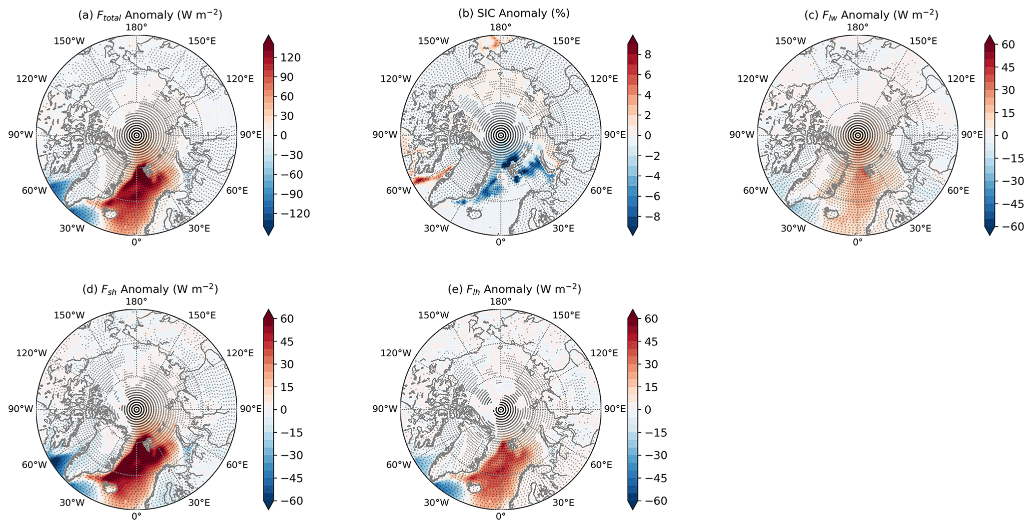
Figure 5 Composite ERA5 anomalies of (a) total surface energy (W m⁻²), (b) sea-ice concentration ( %), (c) surface thermal net irradiance (W m⁻²), (d) surface sensible heat flux (W m⁻²), and (e) surface latent heat flux (W m⁻²) for all EMIs over the Barents Sea, during 1979–2018 winter. The stippling indicates statistical significance at the p<0.01 level from a Student's t test.

A similar surface energy-budget pattern is also found over the Beaufort Sea (Fig. 6) and other ocean sectors with land-locked sea ice (Figs. S2, S4, S6, S8) but with some differences. The anomaly in F_total over the Barents Sea is dominated by F_sh, while F_total anomaly over the Beaufort Sea is dominated by F_lw. The magnitudes of F_sh, F_lh, and F_total anomalies over the Beaufort Sea are less than half the magnitude of those over the Barents Sea, especially south of 80^∘ N and hence induce 4 times less SIC decrease. As EMIs occur over the Beaufort Sea, positive F_sh, F_lh, F_total, F_lw, LWP, and IWP anomalies and negative SIC anomaly is found. However, negative F_sh, F_lh, F_total, F_lw, LWP, and IWP anomalies and positive SIC anomalies could also be found over the Barents Sea sector, while some WaMAIs from the Beaufort Sea pass through the pole and become cold spells over the Barents Sea (Figs. 4 and 6).

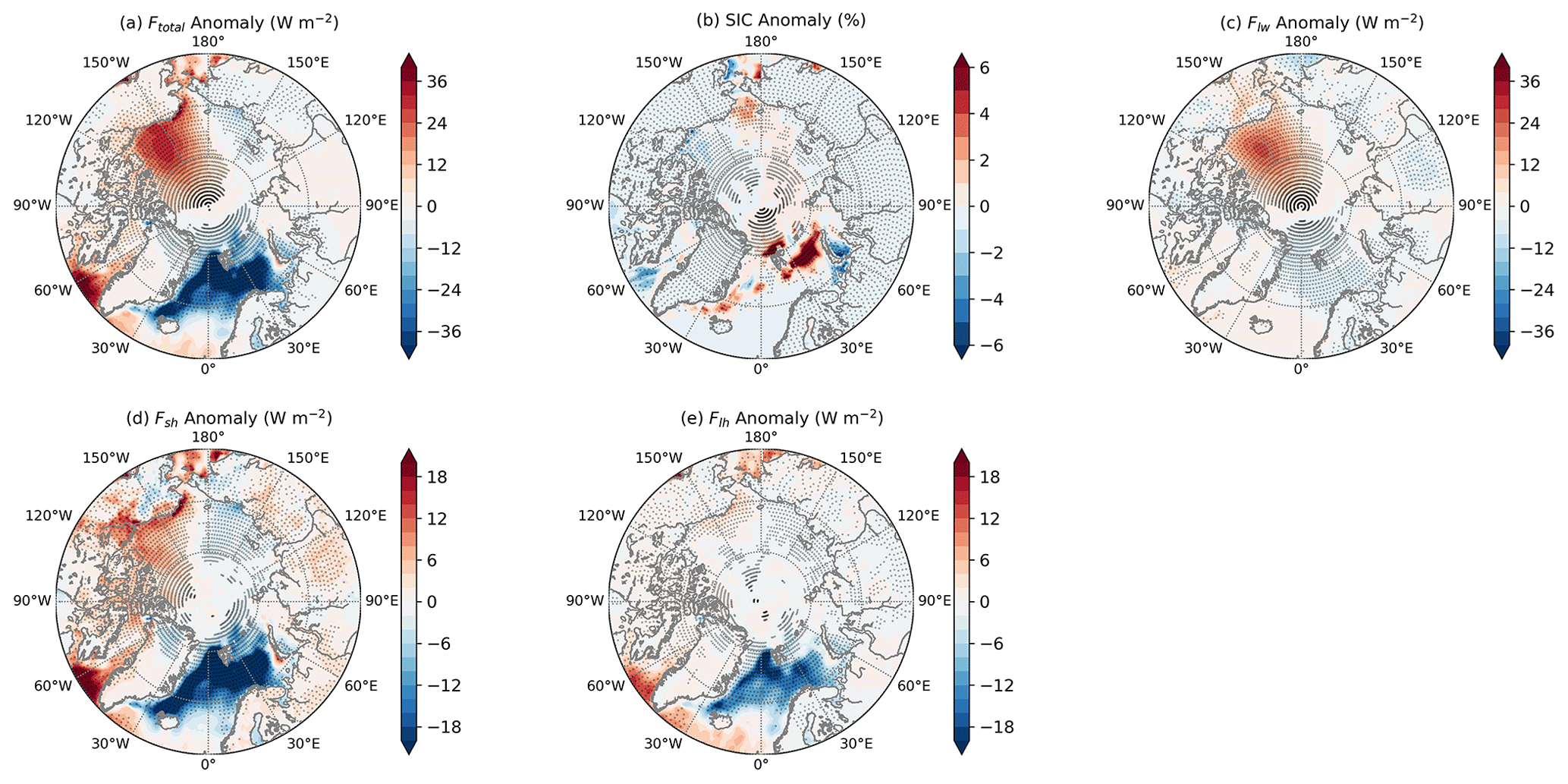
Figure 6 Composite ERA5 anomalies of (a) total surface energy (W m⁻²), (b) sea-ice concentration ( %), (c) surface thermal net irradiance (W m⁻²), (d) surface sensible heat flux (W m⁻²), and (e) surface latent heat flux (W m⁻²) for all EMIs over the Beaufort Sea, during 1979–2018 winter. Noted that the color-bars here are different than those in Fig. 5. The stippling indicates statistical significance at the p<0.01 level from a Student's t test.

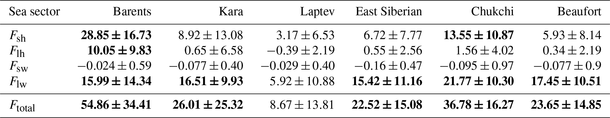
Table 1 summarizes the averaged surface energy-budgets over sea ice across the six basins. Except for the Barents Sea, F_lw anomalies are almost twice larger than F_sh anomalies. Since F_sw anomalies can be ignored in winter, the F_lw anomalies dominate F_total. However, over the Barents Sea, F_sh anomalies are almost twice larger than F_lw anomalies and contribute to more than 50  % of F_total anomalies. Over the Barents Sea and Chukchi Sea, positive F_sh anomalies are statistically significant, which is not the case for any of the other sectors. Except for the Laptev Sea, positive F_total and F_lw anomalies are statistically significant. Here, if the mean values of these surface energy-budget terms are positive and they are still greater than 0 after deducting their standard deviation, then we consider that they are statistically significantly positive. This definition is quite lax, since it only passes 0.32 for Student's significance test.

Table 1 Regional averaged F_sh, F_lh, F_sw, F_lw, and F_total in Kara, Laptev, East Siberian, and Beaufort sectors. The unit is W m⁻² for all variables. Statistically significant positive values are in bold.

The composites of large-scale pattern discussed above are extracted from the stronger EMI events to generate a clear signal; however, these may not necessarily represent the general pattern of all WaMAIs. Therefore, linear regressions of daily averaged GH, T₈₅₀, SIC, F_total, F_sh, F_lh, F_sw, and F_lw anomaly against the time series of daily averaged $\stackrel{\mathrm{‾}}{f_{\mathrm{w}}}$ over the sensitive regions in 40 recent winters were calculated separately for all the examined ocean basins. All the regressed fields have a similar pattern as their counterparts in Figs. 3–6, implying a similar relationship for all days but at smaller magnitudes. Since the regressions confirm the conclusions, we will consider only the Barents Sea and Beaufort Sea as an example of ocean sector with open ocean and land-locked sea ice, respectively (Figs. 7 and 8).

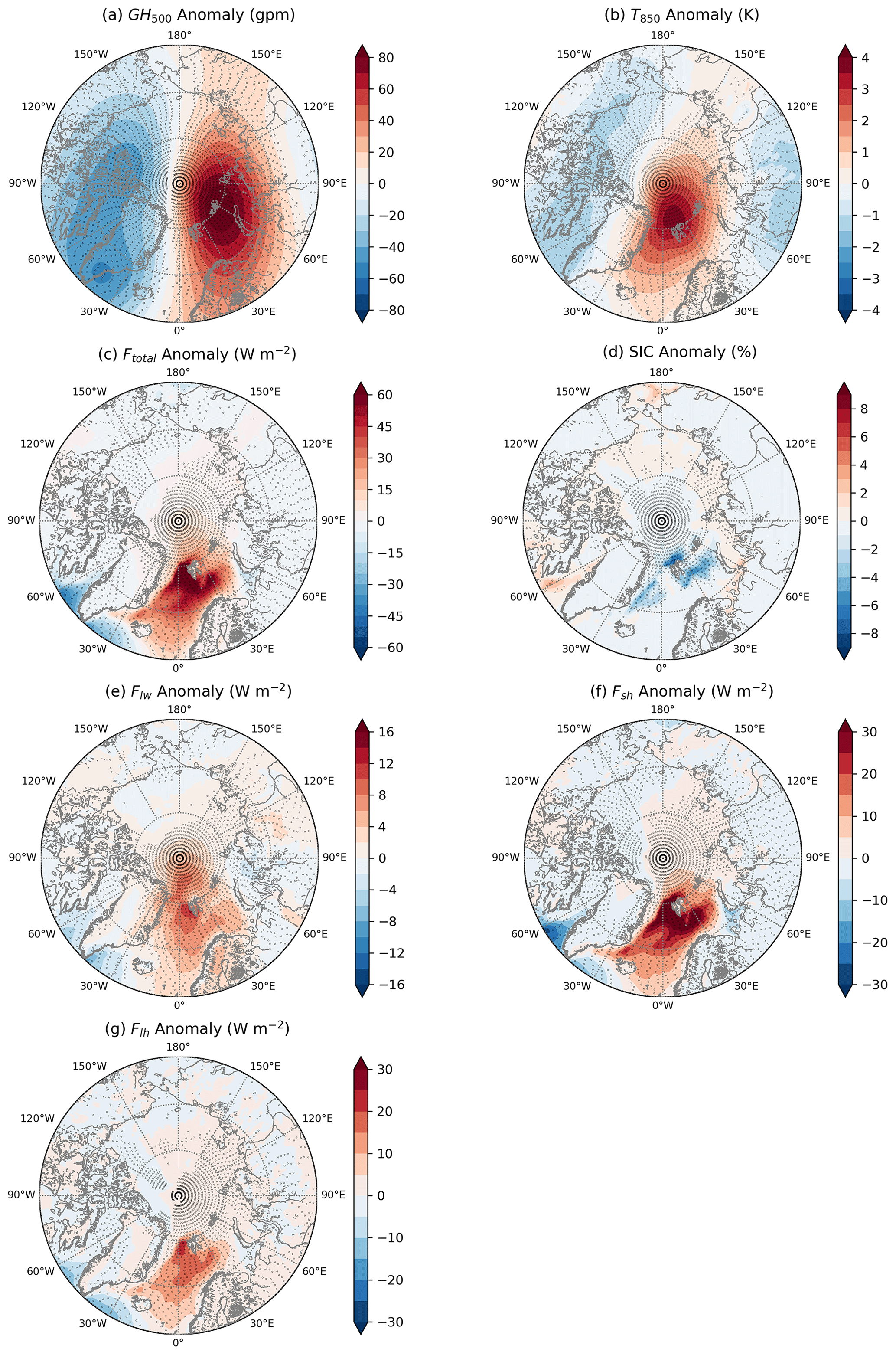
Figure 7 Anomalies of (a) 500 hPa geopotential height (gpm), (b) 850 hPa temperature (K), (c) F_total, (d) SIC, (e) F_lw, (f) F_sh, and (g) F_lh from linear regressions against daily $\stackrel{\mathrm{‾}}{f_{\mathrm{w}}}$ time series over the Barents Sea. The stippling indicates statistical significance at the p<0.05 level from a Student's t test.

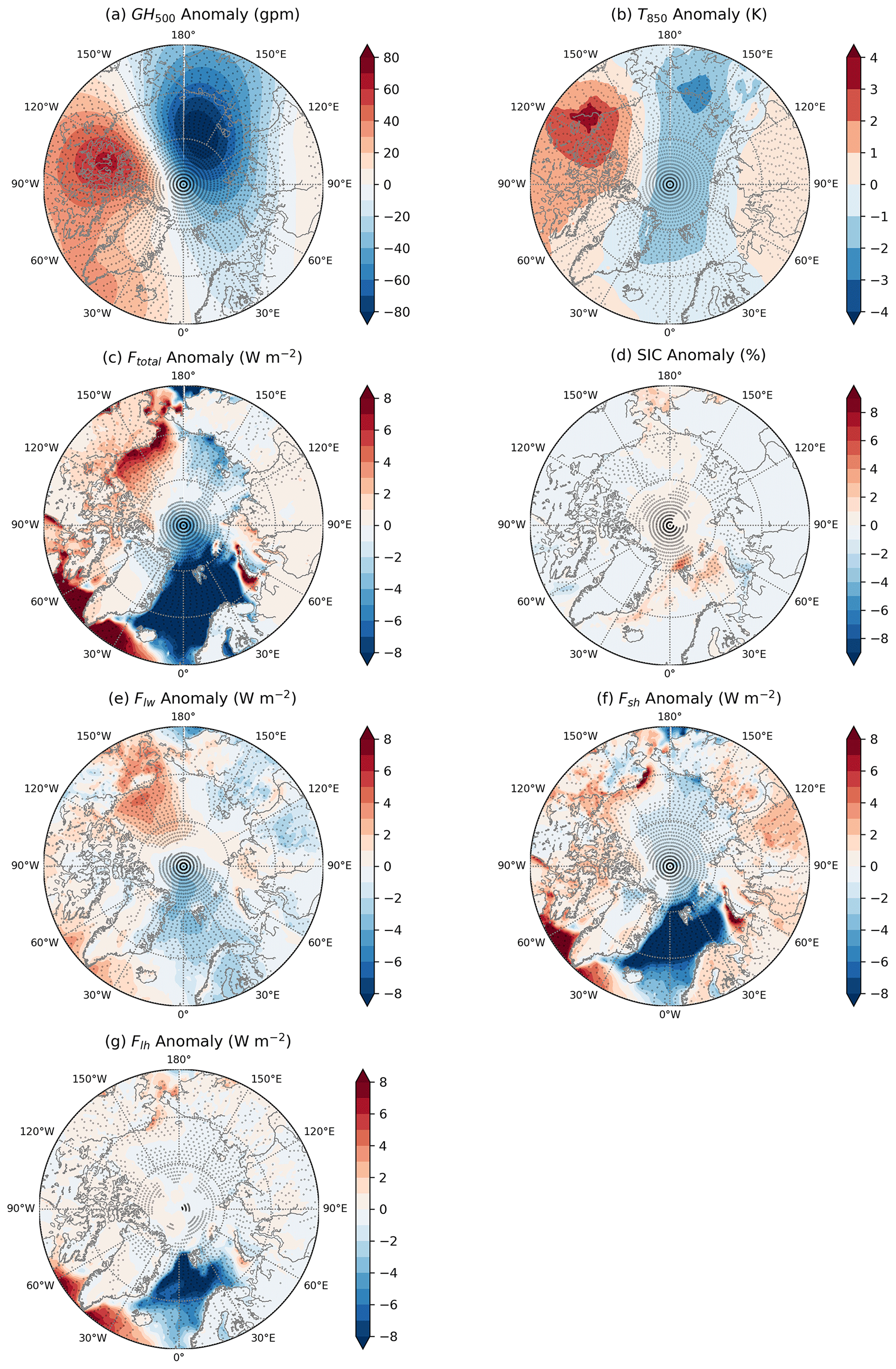
Figure 8 Anomalies of (a) 500 hPa geopotential height (gpm), (b) 850 hPa temperature (K), (c) F_total, (d) SIC, (e) F_lw, (f) F_sh, and (g) F_lh from linear regressions against daily $\stackrel{\mathrm{‾}}{f_{\mathrm{w}}}$ time series over the Beaufort Sea. The stippling indicates statistical significance at the p<0.05 level from a Student's t test. Similarly to Fig. 2a, the linear regressions here are calculated against standardized f_w. Therefore, the unit of the regression is same as the corresponding variables and the values represent the general anomalies from the climate mean during positive f_w.

3.2 The surface energy-budget

In this section, we will explore the transformation of temperature inversion, cloud formation, and surface energy-budget along the trajectories of warm-and-moist air masses over ocean basins with open water and land-locked sea ice, respectively, by compositing the heights to the maximum specific humidity (h_sh), temperature (h_t), and vertical temperature gradient ($h_{{\mathrm{t}}_z}$), along with TWP, LWP, IWP, precipitation rate (PRCP), and surface energy-budget terms (F_sh, F_lh, F_total, F_lw) from all detected WaMAIs.

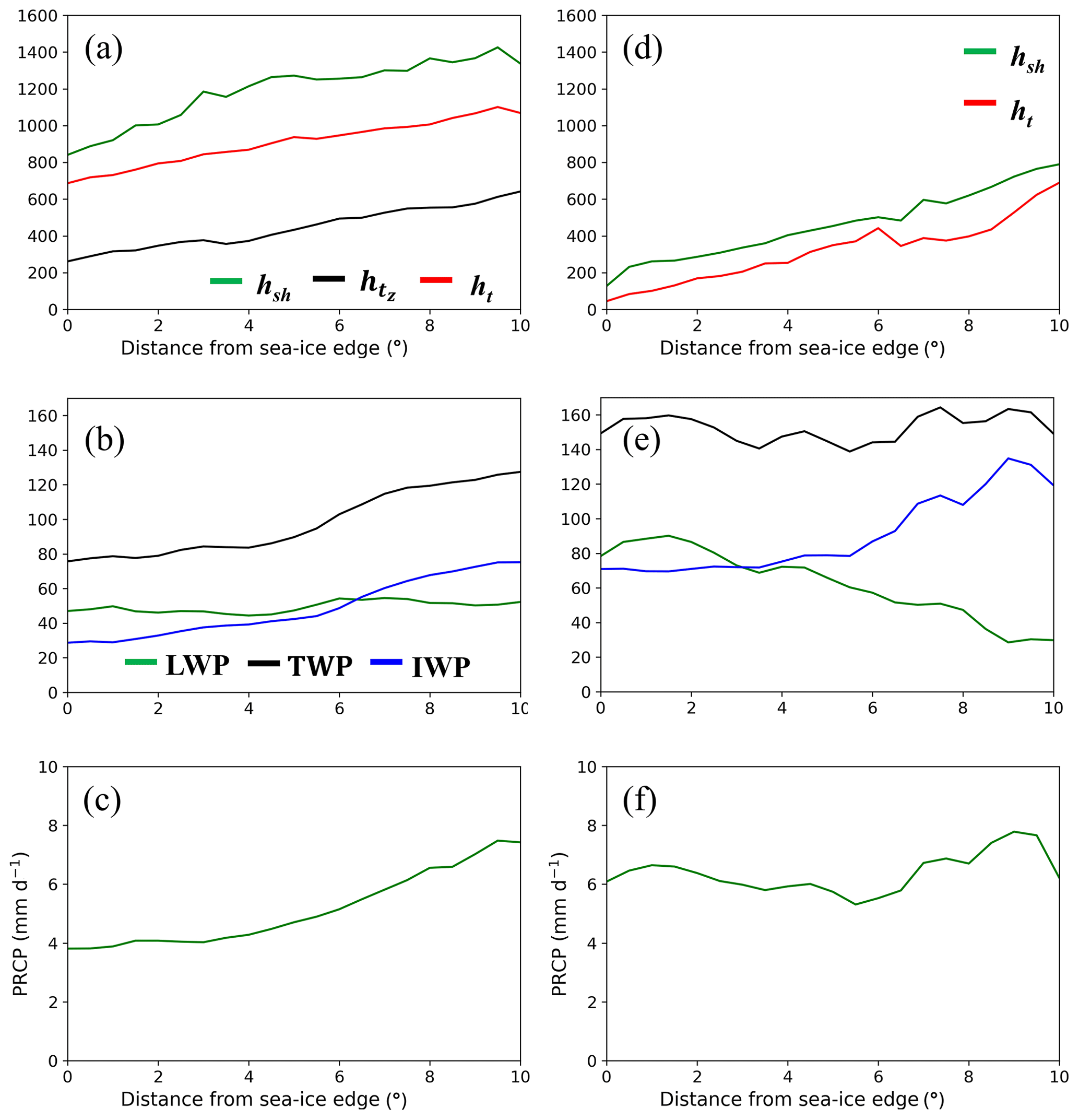
Figure 9 Average variation of (a) the height to the maximum specific humidity (h_sh), temperature gradient ($h_{{\mathrm{t}}_z}$; m), and temperature (h_t); (b) liquid water path (LWP; g m⁻²), ice water path (IWP; g m⁻²), and total water path (TWP; g m⁻²); (c) precipitation rate (PRCP; mm d⁻¹), with the downstream northward distance from sea-ice edge, along the WaMAI trajectories over the Barents Sea. Panels (d), (e), and (f) are the counterparts of panels (a), (b), and (c) over the frozen seas. Note that this is not necessarily the distance traveled, since WaMAIs do not need to travel due northward.

Over the completely ice-covered sea sectors such as the Laptev Sea, East Siberian Sea, Chukchi Sea, and Beaufort Sea, strong temperature inversion develops with cloud formation below, as the warm-and-moist air propagates over the sea ice. In this case, h_sh is higher than h_t, and both are higher than $h_{{\mathrm{t}}_z}$ (Fig. 9a). From the ice edge and onward up to 10^∘ north of the ice edge, h_sh, h_t, and $h_{{\mathrm{t}}_z}$ increase almost linearly, by 30–40 m per degree latitude (Fig. 9a) as the inversion is lifted. TWP and PRCP also increase northward, although more slowly for the first 2^∘, in total by 6 g m⁻² and 0.4 mm d⁻¹ per degree latitude, respectively, implying that stratocumulus develops continuously along the trajectories (Fig. 9b, c). The increasing TWP is mainly due to the increase in IWP since LWP is almost constant along the trajectories (Fig. 9b). The increase of $h_{{\mathrm{t}}_z}$ is comparable to that of summer WaMAIs, while the increase in TWP is about half that of summer WaMAIs (You et al., 2021), since less moisture is available for cloud development in winter (Fig. 4c). The gradual increase of $h_{{\mathrm{t}}_z}$, a manifestation of increased boundary-layer mixing, leads to a reduction in near-surface gradients. Since the turbulent heat fluxes at the surface depend on these gradients, the F_sh anomaly decreases gradually at a rate of 1.5 W m⁻² per degree latitude (Fig. 10a). Simultaneously, the F_lw anomaly increases almost linearly by 2.5 W m⁻² per degree latitude, while F_lh, the smallest contributor to F_total, is almost constant along the trajectories (Fig. 10a). The increase in F_lw along trajectories is due to increasing cloud radiative effects by the evolving stratocumulus clouds; F_{lw_CRE} increases at a similar rate as F_lw (Fig. 10b). From 0 to 2^∘ north of the sea-ice edge, the F_total anomaly is dominated by the F_sh anomaly, while farther north it is dominated by F_lw anomaly (Fig. 10a). Generally, F_total anomaly increases with distance from the sea-ice edge at a rate of 1 W m⁻² per degree latitude, and this increasing trend is dominated by F_lw anomaly (Fig. 10a).

Figure 10 The average meridional evolution in the anomalies of (a) the sum (F_total, W m⁻²; black) and individual surface fluxes of sensible heat (F_sh, W m⁻²; yellow), latent heat (F_lh, W m⁻²; cyan), net longwave irradiance (F_lw, W m⁻²; magenta), and net shortwave irradiance (F_sw, W m⁻²; blue) along the trajectories. Panel (b) shows the cloud radiative effect by longwave irradiance (F_{lw_CRE}; magenta) over the Barents Sea. Panels (c) and (d) are the counterparts of panels (a) and (b) over the frozen seas.

Over the Barents Sea, with open warm water south of the ice edge, h_t and h_sh also increase nearly linearly but at a 1.6 times larger rate than those over ocean sectors with land-locked sea ice but starting at considerably smaller values (Fig. 9d). The maximum values of h_t and h_sp here are comparable to the minimum values over the completely ice-covered sectors, implying that WaMAIs over the Barents Sea develop a shallower well-mixed layer and hence bring the moist and warm air closer to the surface. However, the temperature inversion over the Barents Sea is too weak to be easily identified with the metrics used above. Unlike for the sectors with land-locked sea ice, TWP and PRCP are constant with downwind distance from the ice edge, varying slightly around 150 g m⁻² and 7 mm d⁻¹ (Fig. 9e, f). As a consequence, F_lw anomaly and F_{lw_CRE} along the trajectories (Fig. 10c, d) are nearly constant with northward distance. Although TWP remains quasi-constant, LWP (IWP) decreases (increases) at a rate of −6 g m⁻² (+6 g m⁻²) along the trajectories (Fig. 9e). From 0 to 4^∘ north of the sea-ice edge, TWP is contributed by LWP and IWP in about equal parts, while from 4^∘ north of the sea-ice edge and onward, TWP gradually becomes dominated by IWP. The F_sh anomaly decreases fast by nearly 50 % over the first 2^∘ from the sea-ice edge (Fig. 10c). From 2 to 10^∘ north of the sea-ice edge, the decrease is more moderate at a rate of 4 W m⁻² per degree latitude (Fig. 10c), which is still faster than that over the completely frozen ocean sectors. However, the F_sh anomaly is still larger than the largest corresponding value for the completely frozen ocean sectors, even 10^∘ north of the ice edge (Fig. 10a). This is likely due to the much warmer upstream conditions over the open ocean. The large thermal contrast between open ocean and sea-ice surface contributes to the stable atmospheric layer over the sea-ice surface and rapidly reducing F_sh anomaly, while the decrease of F_sh anomaly with downstream distance is due to the slowly reducing temperature gradient resulting from the turbulent mixing. Similar decreasing trends are also present for F_lh and F_total anomaly (Fig. 10c). From 2 to 10^∘ north of the sea-ice edge, they decrease at a rate of 1 and 5 W m⁻² per degree latitude, respectively (Fig. 10c). Within 5^∘ north of the sea-ice edge, F_total anomaly is dominated by F_sh, while downstream the turbulent heat flux (F_sh+F_lh) anomaly becomes comparable to F_lw anomaly and contributes almost equally to F_total anomaly (Fig. 10c).

Without the presence of solar radiation in winter, the variation of F_total anomaly over the Barents Sea is dominated by F_sh anomaly (Fig. 10a), while it is dominated by F_lw anomaly over ocean sectors with land-locked sea ice (Fig. 10c). This distinction between ocean sectors with and without open ocean upstream can be explained by the stronger air–sea interaction over the Barents Sea (Kim et al., 2019). Before the air mass is advected in over the sea ice, it is heated and moistened by the ocean and consequently exerts greater turbulent heat fluxes on the surface as it suddenly enters over the sea ice (Fig. 10c). Cloud

Cloud formation happens already upstream in a typical cloud-topped marine boundary layer (Lemone et al., 2018) and is hence not much affected by the advection over sea ice. Instead a much shallower well-mixed layer forms as the air enters over the ice, and the larger vertical gradients resulting from the large temperature difference across the ice edge gives rise to larger F_sh. This dominance of turbulent heat fluxes remains until halfway along the trajectories.

3.3 The boundary-layer energy budget

As discussed in previous sections, cloud formation as part of the air-mass transmission can exert large variability on the surface energy-budget. Here, we focus on the cloud effects on the boundary-layer energy budget. For each WaMAI, the boundary-layer energy-budget terms are evaluated and interpolated along the trajectory and analyzed on a case-by-case basis, categorizing patterns into four main categories: (a) lifting temperature inversion (INV), (b) radiation-dominated (RAD), (c) turbulence-dominated (TBL), and (d) turbulence-dominated with cold dome (TCD). Some typical cases are shown in Figs. 11–14, respectively, for these four categories, illustrating different boundary-layer energy budgets in each category, while conceptual summary graphs of all the different categories are summarized in Fig. 15. The boundary-layer energy-budget pattern is very variable from case to case, mainly because the northward component of the advection is different from case to case. Additionally, the location of the ice edge is also different from case to case. Some trajectories are long but reach less far north, while others are shorter but still reach further north. In the vertical, the cases are also subject to different subsidence, affecting the boundary-layer growth. We therefore have not yet come up with a workable idea that would allow for an ensemble average of all the cases.

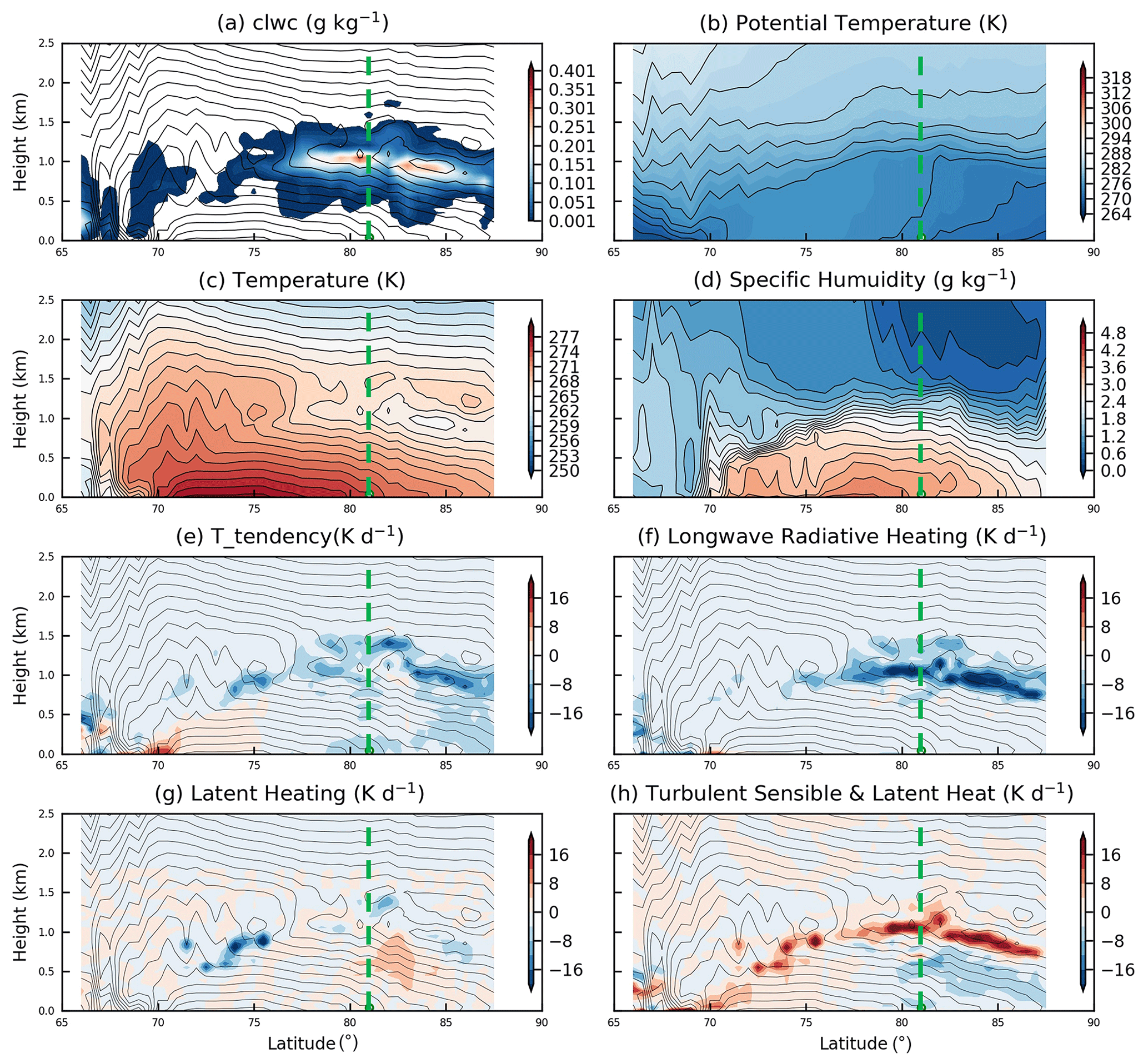
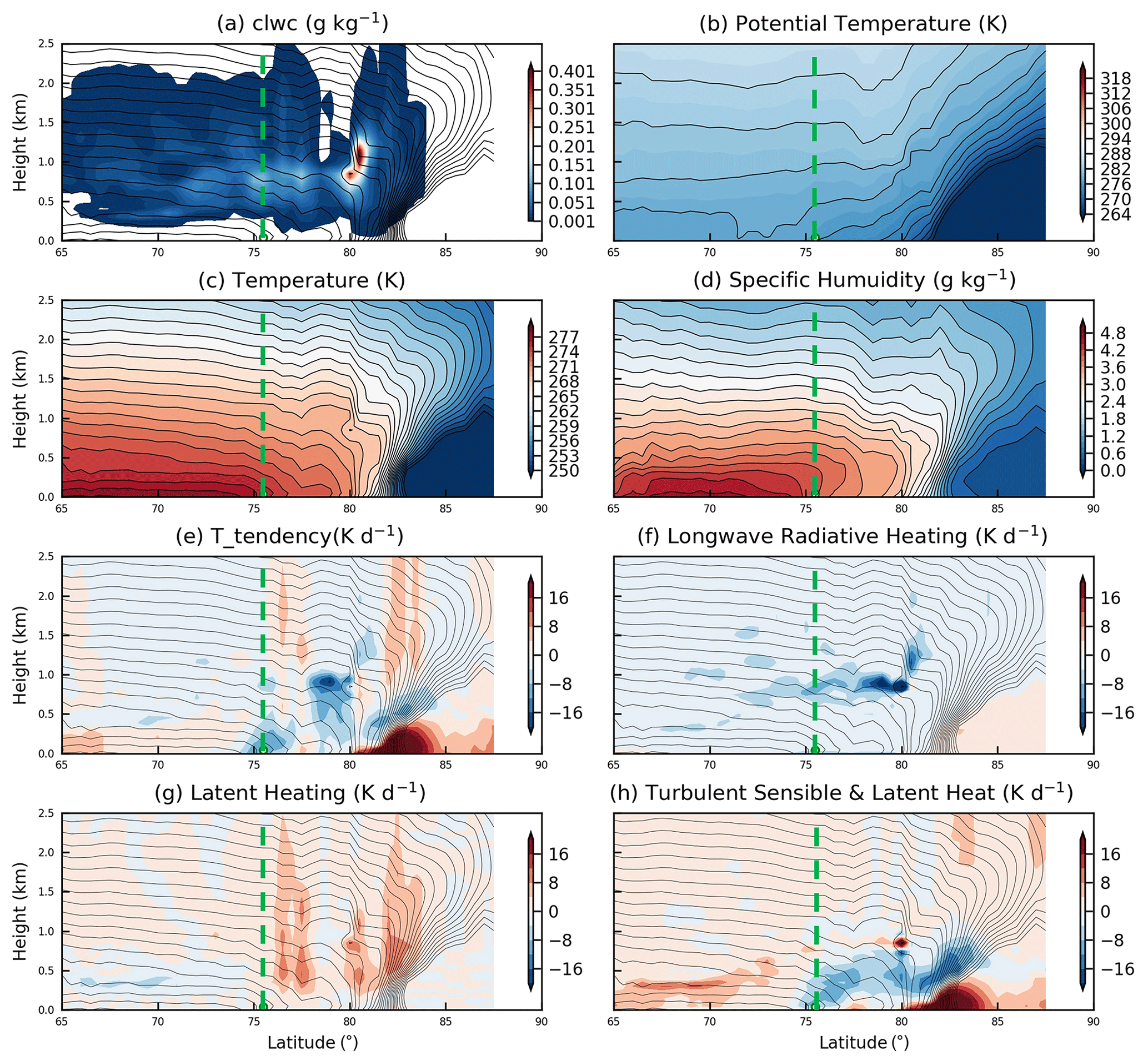
Figure 11 Latitude–height cross-section of (a) cloud liquid water concentration (g kg⁻¹), (b) potential temperature (K), (c) temperature (K), (d) specific humidity (g kg⁻¹), (e) temperature tendency due to model physics (K d⁻¹), (f) longwave radiative heating (K d⁻¹), (g) latent heating (K d⁻¹), and (h) turbulent heating (K d⁻¹), interpolated from ERA5 along trajectories of one selected WaMAI from category INV. The green dashed lines mark the location of the ice edge. See the text for a detailed discussion.

Figure 12 Same as Fig. 11 but for a selected radiation-dominated WaMAI.

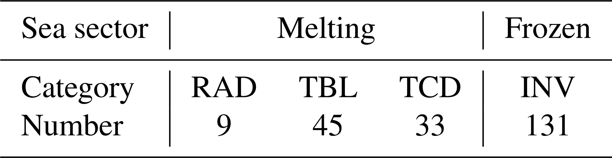
Almost all WaMAIs over ocean sectors with land-locked sea ice feature a boundary-layer energy-budget pattern of category INV. Similar to category TBL for summer WaMAIs (You et al., 2021), category INV is characterized by increasingly lifting temperature inversion and continuously stratocumulus development near the inversion. Different from the ocean sectors with land-locked sea ice, clouds during WaMAIs over the ocean sector with an upstream open ocean (e.g., Barents Sea) form at the altitude of ∼1 km, above the warm-and-moist air masses. The boundary-layer energy budget here is categorized into three categories (RAD, TBL, TCD). Category RAD is characterized by stronger cloud-top radiative cooling and related buoyant mixing, while category TBL is characterized by more intensive surface turbulent mixing. Category TCD is similar to category TBL excluding a cold dome over the high Arctic. The boundary-layer energy-budget patterns are categorized by manually checking case by case if they have the typical characteristics of each category. Their launch time and launch longitudes are listed in Table S1 in the Supplement. WaMAIs over the Kara Sea sectors are characteristic of both ocean sector with land-locked sea ice and open ocean. Some WaMAIs behave as typical for the Barents Sea, while some behave like those for the other sectors with land-locked sea ice.

Note that unlike radiation and condensation/evaporation, turbulence does not generate heating/cooling by itself. Instead, it heats/cools air locally by redistributing heat from one altitude to another through mixing within the column. Also, note that the temperature tendencies discussed below are only those that are due to model physics in a Lagrangian view, while in an Eulerian framework they would be balanced by advection (not shown). In an absolute sense the boundary layer always undergoes a gradual cooling during the advection over the sea ice.

3.3.1 Lifting temperature inversion (INV)

In this category turbulent heating and cooling dominate the boundary-layer energy budget (Fig. 11e and h), even though stratocumulus develops along the trajectories and affects the radiative processes (Fig. 11a and f). Turbulent mixing transports heat from the upper to the lower parts of the PBL and hence cooling the upper and warming the lower parts of the PBL (Fig. 11h). Since the turbulent mixing persists along the trajectories, the well-mixed layer below the inversion continuously deepens northward (Fig. 11b), while the inversion and the cloud top are gradually lifted (Fig. 11a). This supports the hypothesis from Tjernström et al. (2019) that the surface inversion formed at the sea-ice edge is eroded progressively downstream by cloud-top cooling and surface turbulent mixing; eventually, the boundary layer must transform into the often-observed well-mixed cloud-capped boundary layer (Brooks et al., 2017; Graversen et al., 2008; Morrison et al., 2012; Pithan et al., 2014; Sotiropoulou et al., 2014; Tjernström et al., 2012; Tjernström and Graversen, 2009). Even though this hypothesis was originally posed for summer WaMAIs, it is also applicable to winter WaMAIs over completely frozen ocean sectors; see Fig. 15a.

Clouds are relatively thin, and radiative cooling near the cloud top is therefore weak (Fig. 11f); only in a few cases is the magnitude of radiative cooling comparable to the turbulent cooling. Generally, in this category, turbulent heating is larger than radiative heating as well as latent heating; hence, boundary-layer warming is dominated by turbulence, but since turbulence only redistributes heat inside the PBL, as a whole it is gradually cooled as the warm air progresses northward.

3.3.2 Radiation-dominated (RAD)

Over the Barents Sea, the maximum air temperature (Figs. 12a, 13a, 14a) and specific humidity (Figs. 12d, 13d, 14d) over open ocean south of the ice edge are always located right above the sea surface as a result of the strong air–sea interaction and are also typically larger than those over ocean sectors with land-locked sea ice. As this air mass, considerably affected by air–sea interaction, is advected over the sea ice, different stories take place.

Figure 13 Same as Fig. 11 but for a selected turbulence-dominated WaMAI.

Figure 14 Same as Fig. 11 but for a selected turbulence-dominated WaMAI with cold dome.

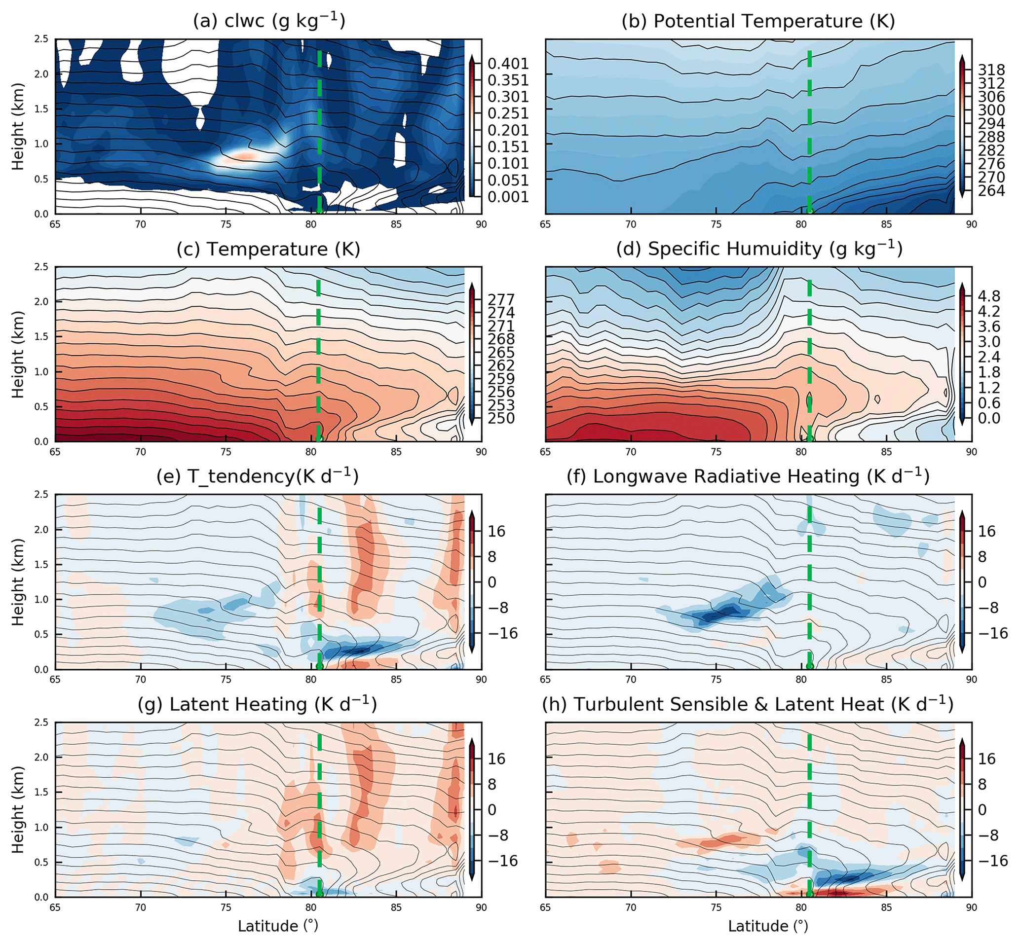
Around 8 % of all WaMAIs over the Barents Sea belong to category RAD (Table 2). In this category, the total temperature tendencies are forced by radiative processes. For this category, the large-scale subsidence is an order of magnitude smaller than that in category TBL (Table 3, CONV), and LWP is 3 times larger than that in category TCD (Table 3, LWP), suggesting that the stratocumulus develops more intensively in category RAD (Fig. 12a). With larger values of LWP, longwave radiation is effectively emitted at the cloud top like a blackbody, exerting large cooling rates with maximum reaching −16 K d⁻¹. However, unlike the cloud formation in category INV, here clouds always already form south of the ice edge over the open water, and few clouds develop in the near-surface inversion. In the cloud, heat is redistributed with warming at the cloud top and cooling in the lower PBL by buoyant mixing driven by cloud-top longwave radiative cooling (Fig. 12h). The turbulent cooling layer in the PBL interior is apparently thicker than the turbulent warming layer whose absolute value of heating rate is considerably more intensive (Fig. 12h). As shown in Fig. 12h, the buoyant mixing can access the surface and induce a thicker well-mixed layer below the stratocumulus (Fig. 12b). As precipitation constantly erodes the cloud, buoyant mixing continuously provides moisture for the cloud development from the moister air below; hence, cloud development as well as the cloud-top cooling is maintained.

Table 2 Number of WaMAIs with boundary-layer energy-budget pattern of category RAD (radiation-dominated), TBL (turbulence-dominated), TCD (turbulence-dominated with cold dome), and INV (lifting temperature inversion) over melting (Barents) and frozen (Laptev, East Siberian, Chukchi and Beaufort) sea sectors.

Meanwhile, the values of maximum temperature and specific humidity are decreasing gradually along the trajectory, indicating that the heat and moisture within the warm-and-moist air is consumed continuously by the cloud formation and surface turbulent mixing. For this category, F_lw is comparable to those of category TBL and TCD (Table 3), and it increases almost linearly along the trajectory (Fig. 16d1) due to the enhancing TWP (Fig. 16c1). F_sh and F_lh are generally smaller than those of category TBL since stronger mixing weakens vertical gradients in the PBL and hence suppresses the surface turbulent heat flux (Table 3). The decreasing rates of F_sh and F_lh from 0 to 2^∘ north of the sea-ice edge are larger than for categories TBL and TCD as a result of stronger buoyant mixing in the PBL (Fig. 16a1), while onwards their decreasing rates are smaller than those for the other two categories since the lifting rates of h_t and h_sp are dramatically slowed down (Fig. 16b1); see Fig. 15b.

Table 3 Averaged F_sh, F_lh, F_sw, F_lw, LWP (from bottom to $h_{{\mathrm{t}}_z}$; g m⁻²), and large-scale convergence (CONV; 10⁻⁵ kg m⁻² s⁻¹) from category TBL and category RAD. Statistically significant positive values are in bold.

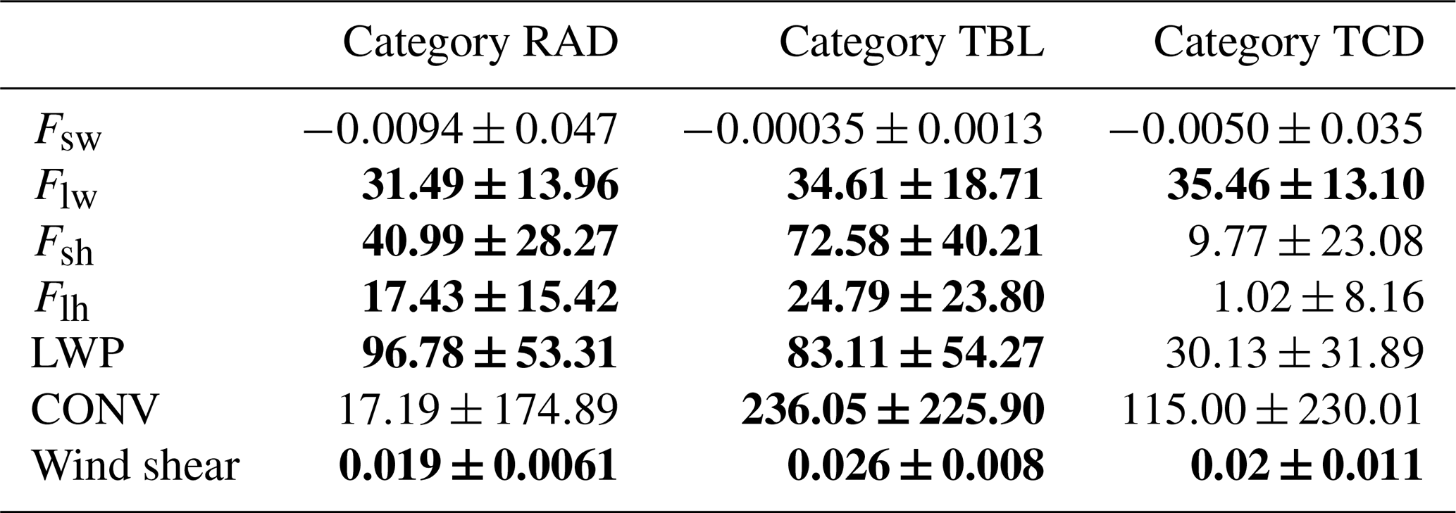
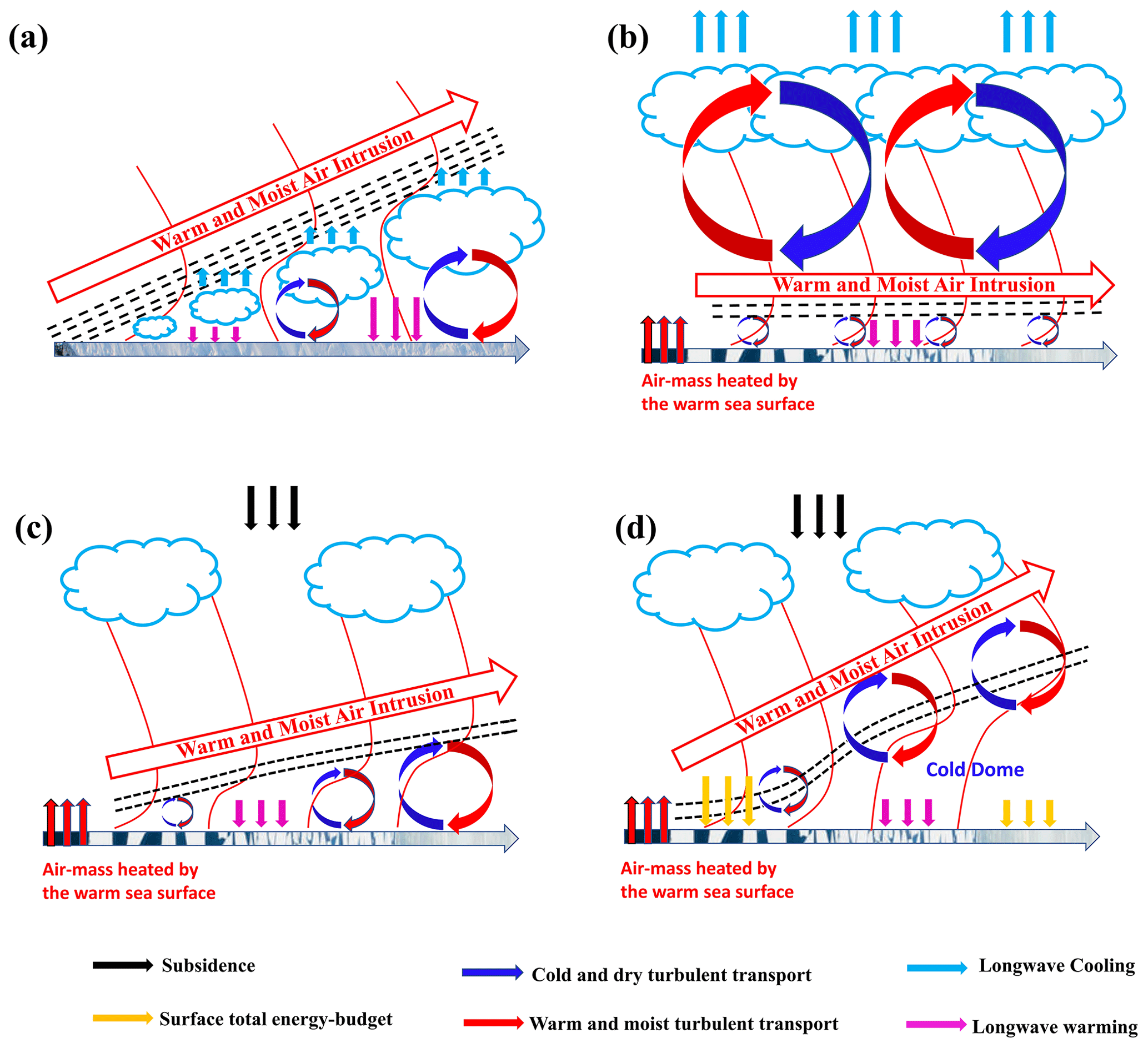
Figure 15 Concept graph of WaMAI from category (a) INV, (b) radiation-dominated WaMAI, (c) turbulence-dominated WaMAI, and (d) turbulence-dominated WaMAI with cold dome. The red lines in (a, b, c) are temperature or humidity profiles. Red arrows represent the WaMAIs. The horizontal arrows represent the Arctic surface with frozen or melting sea ice. Black lines represent inversions.

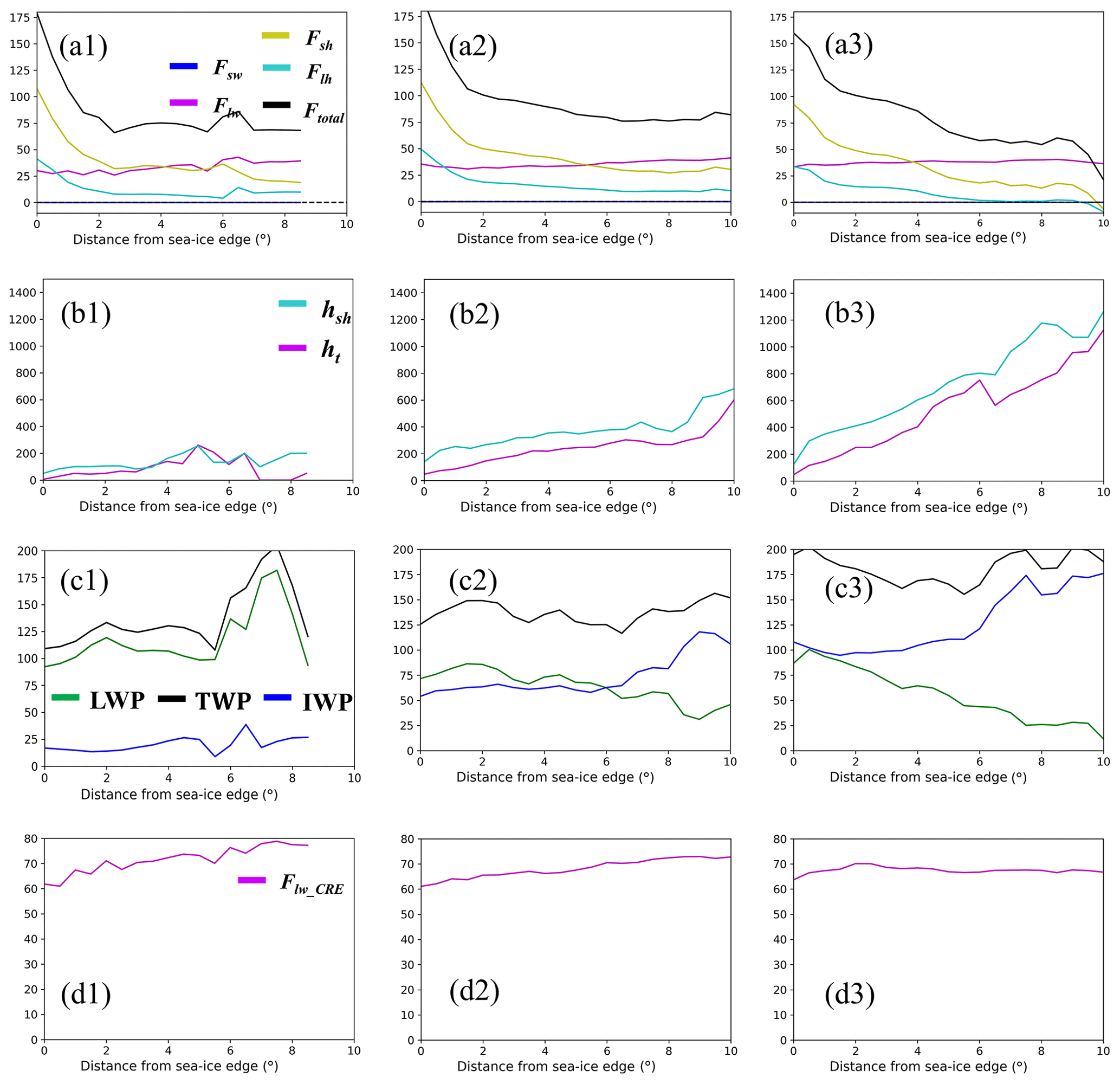
Figure 16 Average variation of (a1) the sum (F_total, W m⁻²; black) and individual surface fluxes of sensible heat (F_sh, W m⁻²; yellow), latent heat (F_lh, W m⁻²; cyan), net longwave irradiance (F_lw, W m⁻²; magenta) and net shortwave irradiance (F_sw, W m⁻²; blue); (b1) the height to the maximum specific humidity (h_sh) and temperature (h_t); (c1) liquid water path (LWP; g m⁻²), ice water path (IWP; g m⁻²) and total water path (TWP; g m⁻²); (d1) the cloud radiative effect by longwave irradiance (F_{lw_CRE}; magenta), with the downstream northward distance from sea-ice edge, along the trajectory of WaMAI in category of RAD over the Barents Sea. Panels (a2), (b2), (c2) and (d2) (a3, b3, c3, d3) are the same but for WaMAIs in category of TBL (TCD).

3.3.3 Turbulence-dominated (TBL)

Fifty-two percent of WaMAIs over the Barents Sea belong to the turbulence-dominated category. The variation of surface energy-budget along the trajectory (Fig. 16a2, b2 and c2) is similar to the mean variation of WaMAIs from all categories shown in Fig. 10c and d. Subsidence for WaMAIs in this category is typically a factor of 3 larger than that in category RAD, and it is statistically significantly positive (Table 3, CONV). Consequently, clouds in this category do not develop as intensively as in category RAD; hence, the radiative cooling rate at the cloud top is considerably smaller. The boundary-layer energy budget is mainly dominated by turbulent heating near the surface. As warm-and-moist air is advected into the Arctic sea ice, turbulence exchanges heat between warm and cold air masses by cooling (heating) warmer (colder) air (Fig. 13h), simultaneously inducing a gradually thickening well-mixed layer capped by a strong inversion, and a continuous lifting of h_t and h_sp (Fig. 13b). In this category, the well-mixed layer is substantially thinner than in category RAD, since the turbulent mixing here is mainly forced by surface friction, which is weaker and less effective than the buoyant mixing in category RAD (Fig. 12b). Turbulence is mainly forced by wind shear and buoyancy, but buoyancy is negative here in the initially very stable near-surface layer. Therefore, wind shear mostly fuels the turbulent mixing. In category TBL, turbulent mixing is stronger than in category RAD, but the surface fluxes are still stronger, due to the stronger gradients; F_sh and F_lh are 77 % and 42 % larger than those in category RAD. Also see Fig. 15c.

3.3.4 Turbulence-dominated with cold dome (TCD)

Forty percent of WaMAIs over the Barents Sea belong to this category. For this category, the boundary-layer energy budget is generally similar to that in category TBL. The main difference is that there is always a layer of cold air (cold dome) laying below the warm-and-moist air mass especially in the central Arctic (Fig. 14c). This cold dome enlarges the vertical temperature gradient and hence intensifies turbulent heat near the surface (Fig. 14h). As the warm-and-moist air mass is advected over the cold dome, it is gradually lifted up by the cold dome and consequently h_t and h_sp are increasing at a faster rate than in category TBL (Fig. 16b3). With faster lifting of h_t and h_sp, F_sh and F_lh would be reduced more rapidly or even become negative in the high Arctic (Fig. 16a3). TWP is dominated by LWP in category RAD, and TWP is contributed almost equally by LWP and IWP in category TBL, while in category TCD, TWP is gradually more dominated by IWP; the IWP-to-TWP ratio increases linearly from ∼50 % to ∼100 % (Fig. 16c3); also see Fig. 15d.

4 Conclusion

The warm Arctic in winter is always related with long-lived blocking (Luo et al., 2017b, 2018). To the west of these blocks, warm-and-moist air is transported to the Arctic, greatly contributing to Arctic surface warming. In this research, we name these warm events as warm-and-moist air intrusions (WaMAIs). As the persistence of Arctic blocking increases (Luo et al., 2017b), WaMAIs could be more frequent and hence lead to more amplified Arctic warming in winter (You et al., 2022). To understand the surface and boundary-layer energy budget as WaMAIs occur, in this paper, we have detected WaMAIs over the Arctic Ocean sectors of Barents, Kara, Laptev, East Siberian, Chukchi, and Beaufort in 40 recent winters (DJF from 1979 to 2018) using the ERA5 reanalysis. The climatological analysis shows a consistent pattern with a blocking high-pressure system over corresponding ocean sectors leading to warm-and-moist air intrusions into the winter Arctic, supplying moisture for cloud formation and exerting a positive total energy-budget anomaly on the surface.

Statistically, as warm-and-moist air is advected over ocean sectors with land-locked ice cover (such as the Laptev Sea, East Siberian Sea, Chukchi Sea, and Beaufort Sea), the longwave irradiance anomaly increases linearly by 2.5 W m⁻² per degree latitude, while the total column cloud liquid water increases linearly by 6 g m⁻² per degree latitude. The longwave irradiance is dominant in the surface energy-budget. We have also analyzed the boundary-layer vertical structure along these trajectories, as well as the associated surface energy-budget pattern of over these sectors, and we find one main category: elevated lifting temperature inversion (INV), which in structure is similar to summer WaMAIs (You et al., 2021) (Fig. 15a).

During WaMAIs over the Barents Sea where open water exists to the south of the sea-ice edge, turbulent heat flux is dominant over the surface energy-budget, especially along the first half-way of the trajectories (Fig. 10c). This difference on the surface energy-budget between the Barents Sea and frozen sea sectors is also preliminarily discussed by Lee et al. (2017). Three main categories are found; radiation-dominated (category RAD), turbulence-dominated (category TBL), and turbulent-dominated with cold dome (category TCD), comprising 8  %, 52  %, and 40  %, respectively, of all WaMAIs. Unlike over the sectors with land-locked sea ice, air masses over the ice-free Barents Sea are warmed by the sea surface (local process) before being advected over the sea ice (remote process), consequently resulting in more intensive surface warming.

In response to 10 times smaller large-scale subsidence, stratocumulus develop more strongly in category RAD with more intensive cloud-top radiative cooling, inducing an apparently thicker well-mixed layer (Fig. 15b). However, this strong radiative cooling induces intensive buoyant mixing extending from the cloud top till the surface, which suppresses the surface turbulent mixing and decreases the lifting rate of the height to the maximum temperature (h_t) and to the maximum specific humidity (h_sp). Therefore, surface turbulent fluxes in category RAD and the lifting rate of h_t and h_sp are apparently smaller than those in category TBL (Fig. 15c). With cold dome, less liquid cloud water could be formed and fewer or even negative turbulent fluxes could access the surface, in comparison with category TBL (Fig. 15d). In category TCD, turbulent fluxes decrease faster along the trajectory since warm-and-moist air is lifted to higher altitude above the cold dome (Fig. 15d).

Under the background of global warming, the rate of this local process has been accelerated by 9  % yr⁻¹ (Kim et al., 2019), while the meridional heat and moisture transports (remote processes) over the Barents Sea are also enhanced in recent decades (Nygård et al., 2020). This implies that WaMAI may play a more significant role in the future Arctic warming. Therefore, the potential mechanism which enhances the occurrence and intensity of WaMAI deserves more attention from atmospheric scientists.