Satellite soil moisture data assimilation impacts on modeling weather variables and ozone in the southeastern US – Part 2: Sensitivity to dry-deposition parameterizations

Ozone (O₃) dry deposition is a major O₃ sink. As a follow-up study of Huang et al. (2021), we quantify the impact of satellite soil moisture (SM) on model representations of this process when different dry-deposition parameterizations are implemented, based on which the implications for interpreting O₃ air pollution levels and assessing the O₃ impacts on human and ecosystem health are provided. The SM data from NASA's Soil Moisture Active Passive mission are assimilated into the Noah-Multiparameterization (Noah-MP) land surface model within the NASA Land Information System framework, semicoupled with Weather Research and Forecasting model with online Chemistry (WRF-Chem) regional-scale simulations covering the southeastern US. Major changes in the modeling system used include enabling the dynamic vegetation option, adding the irrigation process, and updating the scheme for the surface exchange coefficient. Two dry-deposition schemes are implemented, i.e., the Wesely scheme and a “dynamic” scheme, in the latter of which dry-deposition parameterization is coupled with photosynthesis and vegetation dynamics. It is demonstrated that, when the dynamic scheme is applied, the simulated O₃ dry-deposition velocities v_d and their stomatal and cuticular portions, as well as the total O₃ fluxes F_t, are larger overall; v_d and F_t are 2–3 times more sensitive to the SM changes due to the data assimilation (DA). Further, through case studies at two forested sites with different soil types and hydrological regimes, we highlight that, applying the Community Land Model type of SM factor controlling stomatal resistance (i.e., β factor) scheme in replacement of the Noah-type β factor scheme reduced the v_d sensitivity to SM changes by ∼75 % at one site, while it doubled this sensitivity at the other site. Referring to multiple evaluation datasets, which may be associated with variable extents of uncertainty, the model performance of vegetation, surface fluxes, weather, and surface O₃ concentrations shows mixed responses to the DA, some of which display land cover dependency. Finally, using model-derived concentration- and flux-based policy-relevant O₃ metrics as well as their matching exposure–response functions, the relative biomass/crop yield losses for several types of vegetation/crops are estimated to be within a wide range of 1 %–17 %. Their sensitivities to the model's dry-deposition scheme and the implementation of SM DA are discussed.

1 Introduction

Ground-level ozone (O₃) is a regulated secondary air pollutant harmful to human and ecosystem health (Fleming et al., 2018; Mills et al., 2018a, b). It is closely connected with O₃ at higher altitudes where O₃ plays a more important role in the Earth's climate system by trapping infrared radiation and absorbing ultraviolet radiation (e.g., Lacis et al., 1990). To better protect human health and public welfare, in 2015, the US primary and secondary National Ambient Air Quality Standards were lowered from 75 to 70 ppbv, in the format of daily maximum 8 h average (MDA8). Several other O₃-exposure-based metrics have also been applied and/or proposed to assess O₃ impacts on vegetation, such as the accumulated O₃ exposure over given thresholds (e.g., SUM40, SUM60, and AOT40), the averaged O₃ exposure during daylight hours (e.g., M7 and M12), and the sigmoidal-weighted W126 cumulative exposure (e.g., Fredericksen et al., 1996; van Dingenen et al., 2009; Hemispheric Transport of Air Pollution, 2010, and references therein; Avnery et al., 2011; Hollaway et al., 2012; Huang et al., 2013; Lapina et al., 2014; Mills et al., 2007, 2018a, b). To help comply with the tighter air quality standards, an improved understanding of the individual processes affecting the (near-)surface O₃ concentrations and exceedances is demanded. Many O₃-related processes are highly sensitive to environmental and/or biophysical conditions (e.g., Steinkamp and Lawrence, 2011; Strode et al., 2015; Jiang et al., 2018; Huang et al., 2021, and references therein). These O₃-related processes include dry deposition of O₃ and its precursors, which is a major sink for near-surface O₃ and depends on dry-deposition velocities (v_d) and the deposited chemicals' concentrations (Baublitz et al., 2020; Huang et al., 2021). As recognized in numerous studies, accurately estimating dry-deposition fluxes is critical to understanding O₃ budgets and exceedances in the past, present, and future (e.g., Stevenson et al., 2006; Griffiths et al., 2021); moreover, it could contribute to a more reasonable assessment of the O₃ impacts on vegetation (e.g., Mills et al., 2011; Lombardozzi et al., 2015; Mills et al., 2018a; Ducker et al., 2018; Ronan et al., 2020; Fu et al., 2022), which is also relevant to the budgets of other greenhouse gases, weather, and climate.

Ozone uptake by plants is generally higher in warm/growing seasons and during the daytime when O₃ concentrations and v_d values peak. As introduced in Huang et al. (2021) and references therein, over the land, surface resistance r_c, which is composed of stomatal–mesophyll (r_s–r_m), cuticular (r_lu), in-canopy, and ground resistance terms, often exerts the strongest effects on the magnitude and variability of v_d. v_d also includes the aerodynamic resistance (r_a) and quasi-laminar sublayer resistance (r_b) terms.

Soil moisture (SM) and its variability impact v_d in the following ways: (1) SM can play a key role in controlling the opening and closing of plants' stomata as well as the mesophyll functioning (Egea et al., 2011; Baillie and Fleming, 2019), and thus it can directly affect the r_s and r_m terms of v_d. (2) SM is closely linked with vegetation attributes, such as the growing-season above-ground biomass, which is often expressed as leaf area index (LAI) or vegetation optical depth (VOD) and controls the stomatal and cuticular uptake of O₃-related species. (3) SM as well as vegetation conditions can affect multiple v_d terms through its interactions with other environmental conditions (e.g., temperatures, radiation, precipitation, and humidity fields) that modulate these v_d terms, and such effects are generally stronger over transitional climate zones located between dry and wet climates. The SM impacts on v_d and atmospheric states through the above-mentioned pathways are likely to continue to grow in future. This is because, according to Intergovernmental Panel on Climate Change (2021), the occurrence and severity of droughts, some of which are characterized by surface and/or column-averaged SM deficits, are projected to increase over many US regions under warmer future environments. Better understanding the potentially enhanced SM dependency of dry deposition and weather conditions under the changing climate is important because O₃ stress, together with heat, water, and other stresses, can pose more complex threats to plant health than single stress alone (Otu-Larbi et al., 2020).

Single-point models and three-dimensional chemical transport models have long been used to estimate v_d values and their responses to climate change. In the widely used, empirical Wesely scheme (Wesely, 1989), v_d is sensitive to only a few meteorological variables, with SM and plants' physiological effects ignored. In previous studies, Wesely-scheme-based v_d fluxes as well as their various terms from different global, regional, and point-scale modeling systems were intercompared and/or evaluated with v_d and r_s observations from sparsely distributed sites (e.g., Val Martin et al., 2014; Hardacre et al., 2015; Clifton et al., 2017; Silva and Heald, 2018; Wu et al., 2018; Lin et al., 2019) in terms of their magnitude and variability. Studies such as Hardacre et al. (2015) show that, even when similar (Wesely and Wesely-like) v_d schemes were applied, various models behaved differently in calculating v_d, reflecting the impacts of land use and land cover (LULC) and meteorological fields which depend on the individual models' configurations (e.g., scales, inputs). In almost all above-cited studies, large model–model and model–observation discrepancies (i.e., by a factor of 2 or more) have been found in places, suggesting the strong need of diagnosing and addressing issues in the models' configurations and dry-deposition parameterizations.

Revised or alternative dry-deposition schemes have been applied in an increasing number of global- and regional-scale modeling studies. In some of these works, stomatal conductance is calculated based on one-big-leaf multiplicative algorithms that are more complicated than the Wesely (1989) approach, in the way that the empirical maximum stomatal conductance is adjusted by more factors, including water availability and vegetation attributes (e.g., Anav et al., 2018; Falk and Søvde Haslerud, 2019; Emmerichs et al., 2021). In others, v_d calculations are coupled with photosynthesis and vegetation phenology (e.g., Val Martin et al., 2014; Wu et al., 2018; Lin et al., 2019; Wong et al., 2019; Clifton et al., 2020), which in this paper are frequently referred to as “dynamic” schemes. Such types of modifications have been the recommended directions for improving the estimates of v_d as well as the v_d and O₃ responses to climate change, in that they have been demonstrated to be capable of enhancing the dynamics and reducing the systematic biases of the modeled v_d. However, results based on such updated v_d schemes are still associated with variable extents of uncertainty due to limitations in model parameterizations (related to structures, empirical parameters, and stress functions) and/or configurations. In some existing works that applied the dynamic schemes, such uncertainty was quantified and addressed by simply scaling the fluxes resulting from the dynamic schemes towards flux measurements available at very limited locations during non-recent time periods (e.g., Val Martin et al., 2014). These types of modified dry-deposition schemes still require further investigations and optimizations, which can be approached by (1) quantifying the sensitivities of process-based model variables to SM and other environmental and/or biophysical variables for various LULC and soil types; (2) improving model representations of processes central to SM states and land–atmosphere interactions, such as including irrigation and other human activities, tuning physics schemes (e.g., those related to the surface exchange coefficient, C_H) in land surface models (LSMs), and using available observations to constrain (some of) the key land variables in models; and (3) including a wide range of observations and/or observation-derived carbon, water, and energy fluxes as well as vegetation states in model evaluation for broad geographical regions. Furthermore, it is important to explicitly connect the progress in dry-deposition modeling with the impact assessments of O₃ and other air pollutants on ecosystem health, productivity, and diversity.

A regional-scale land modeling and SM data assimilation (DA) framework coupled with weather and atmospheric chemistry modeling by the Weather Research and Forecasting model with online Chemistry (WRF-Chem) is implemented in this work. Using this tool, we quantify and discuss the responses of v_d and its key components as well as O₃ concentrations and plant uptake to SM changes due to the DA, for different soil texture, LULC, and crop types. The central parts of this work rely on the Noah-Multiparameterization (Noah-MP; Niu et al., 2011) LSM with dynamic vegetation that enables the implementation of a modified dynamic dry-deposition scheme. This implemented dynamic scheme couples the r_s calculation with photosynthesis for sunlit and shaded leaves and the r_lu calculation with vegetation phenology. With this modified scheme, both the indirect (i.e., via changing weather and vegetation fields) and direct effects of SM on dry deposition are considered in this modeling system. Results based on this modified scheme and the WRF-Chem default Wesely scheme are compared and evaluated with independent datasets. As an extended work of Huang et al. (2021), here we continue to focus on the southeastern US during summer 2016 for which period prior Noah- and Wesely-based model calculations were conducted and aircraft observations are available. This paper introduces the applied two dry-deposition schemes in Sect. 2. It then presents SM and vegetation states (Sect. 3.1), surface fluxes, and weather fields (Sect. 3.2) from this Noah-MP-based modeling system, in comparison with those from Huang et al. (2021). Discussions on O₃ concentrations and fluxes based on all related WRF-Chem simulations are also connected with the assessment of O₃ impacts on societies, ecosystem health, and crop yield (Sect. 3.3). Summary and suggestions on future directions are provided in Sect. 4.

2 Methods

2.1 Modeling and DA experiment design

The modeling tools and DA experiment design of this study were largely consistent with the Huang et al. (2021) study: we conducted model simulations over the southeastern US in a semicoupled Land Information System (LIS)–WRF-Chem system without and with the assimilation of the enhanced SM retrievals from NASA's Soil Moisture Active Passive (SMAP; Entekhabi et al., 2010) mission. Two dry-deposition schemes (details in Sect. 2.3) were applied in cases without and with the SM DA. The 12 km/63 vertical layer Lambert conformal grid, atmospheric/land initialization, and SM DA methods were adapted from our previous study based on the Noah LSM. Major model input datasets and physics and chemistry schemes were kept similar to before except a few aspects relevant to the upgrade of LSM from Noah to Noah-MP (version 3.6) and the implementation of an irrigation scheme to be introduced in Sect. 2.2.

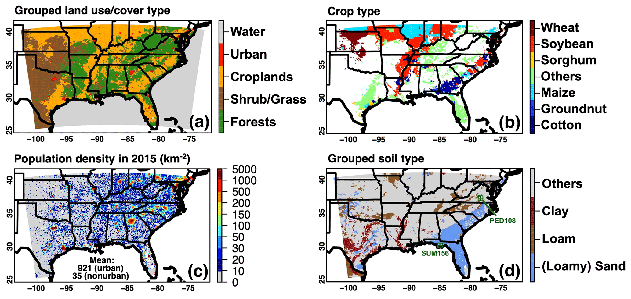
Figure 1 (a) Grid-dominant land use/land cover types grouped from the original 20-category model input (Fig. 1c in Huang et al., 2021) based on the method in Table S1, (b) grid-dominant crop type over cropland-dominant regions, (c) gridded population density in 2015, and (d) highlighted grid-dominant soil types of sand/loamy sand, loam, and clay which are most relevant to discussions in this paper. The original soil type input from the State Soil Geographic database is shown in Fig. S1 in Huang et al. (2021). Locations of the two CASTNET sites for the case studies are denoted in green.

As in Huang et al. (2021), the LULC and soil texture type inputs of our coupled modeling system were based on the International Geosphere-Biosphere Programme-modified Moderate Resolution Imaging Spectroradiometer dataset (Table S1) and the State Soil Geographic dataset, respectively. Crop type data from Monfreda et al. (2008) were used in the irrigation scheme and the assessment of the O₃ impacts on vegetation (Fig. 1b), which are roughly consistent with the 2016 records from the US Department of Agriculture National Agricultural Statistics Service for several major crops such as maize, soybean, and wheat (https://nassgeodata.gmu.edu/CropScape, last access: 8 November 2021). In Sect. 3 of this paper, model results are summarized and/or discussed by groups of grid-dominant LULC and soil type that are shown in Fig. 1a and d. The original 20 LULC types were grouped into urban and non-urban areas and for vegetation-dominant areas, into forests, croplands, and shrub/grasslands, following the criteria introduced in Table S1. The grid-dominant LULC groups for vegetated regions used in our analysis are vastly similar to independently developed data products, e.g., a dataset derived from the European Space Agency–Climate Change Initiative Land Cover project (https://gwis.jrc.ec.europa.eu/apps/country.profile/overview/USA, last access: 8 November 2021) and the 2016 National Land Cover Database (Wickham et al., 2021). Urban-dominant grid cells are well aligned with dense population areas (Fig. 1c) based on the Gridded Population of the World version 4.11 (NASA Socioeconomic Data and Applications Center, 2018). Grid-scale discrepancies exist between the LULC input used and independent LULC products, which, however, are not anticipated to considerably impact the results averaged by LULC groups. Three groups of soil are highlighted, namely sand/loamy sand, loam, and clay. The original sand and loamy sand categories are combined because of their high sand fractions (http://www.soilinfo.psu.edu/index.cgi?soil_data&conus&data_cov&fract&methods, last access: 10 December 2021).

2.2 Physics and configurations of the Noah-MP LSM

The Noah-MP LSM includes a number of improvements from Noah, and one of the enhanced features in Noah-MP is that it contains a separate canopy layer that explicitly computes photosynthetically active radiation, canopy temperature, and related energy, water, and carbon fluxes so that it facilities a dynamic vegetation model. A modified two-stream radiation transfer scheme was used to compute fractions of sunlit and shaded leaves and their absorbed solar radiation. The Ball–Berry type of r_s scheme (e.g., Ball et al., 1987) was applied as required by the dynamic vegetation option. When this option is used, the green vegetation fraction (GVF) does not come from an input dataset as in Huang et al. (2021) but is related to the LAI based on Eq. (1):

$$\begin{array}{}\text{(1)}& \mathrm{GVF}=\mathrm{1}-e^{-\mathrm{0.52}\mathrm{LAI}}.\end{array}$$

Niyogi and Raman (1997) concluded that Ball–Berry, along with two other physiological schemes, performed better on r_s than the multiplicative Jarvis type, which has been frequently used with the prescribed vegetation option. Specifically, it helps better capture the variance in r_s and is more responsive to environmental changes. As described in Appendix B of Niu et al. (2011), this scheme relates stomatal resistance r_s,i of sunlit and shaded leaves i to the photosynthesis rates (A_i) per unit LAI of sunlit and shaded leaves i separately:

$$\begin{array}{}\text{(2)}& {\displaystyle \frac{\mathrm{1}}{r_{\mathrm{s},i}}}=m{\displaystyle \frac{A_i}{C_{\mathrm{air}}}}{\displaystyle \frac{e_{\mathrm{air}}}{e_{\mathrm{sat}}\left(\text{TV}\right)}}{P}_{\mathrm{air}}+g_{\min },\end{array}$$

where C_air is CO₂ concentration at the leaf surface. For our study period, this was set at 400 ppmv according to the median value of Atmospheric Carbon and Transport (ACT)-America B-200 aircraft near-surface (i.e., >900 hPa) CO₂ observations, which is close to the global monthly-mean CO₂ concentrations in August 2016 (https://gml.noaa.gov/webdata/ccgg/trends/co2/co2_mm_gl.txt, last access: 8 November 2021); TV, P_air, e_air, and e_sat(TV) are canopy temperature, surface air pressure, vapor pressure at the leaf surface, and saturation vapor pressure inside leaf, respectively; g_min and m are land-cover-dependent empirical parameters. A_i is determined by Eqs. (3)–(6):

$$\begin{array}{}\text{(3)}& {\displaystyle }{A}_i=I_{\mathrm{gs}}\min (A_{\mathrm{C}},A_{\mathrm{L},i},A_{\mathrm{S}})\text{(4)}& {\displaystyle }{A}_{\mathrm{C}}={\displaystyle \frac{(c_i-c_{\mathrm{cp}})V_{\max }}{c_i+K_{\mathrm{c}}(\mathrm{1}+\frac{o_i}{K_{\mathrm{o}}})}}\text{(5)}& {\displaystyle }{A}_{\mathrm{L},i}={\displaystyle \frac{\left(c_i-c_{\mathrm{cp}}\right)\mathrm{4.6}\mathit{\alpha }{\text{PAR}}_i}{c_i+\mathrm{2}{c}_{\mathrm{cp}}}}\text{(6)}& {\displaystyle }{A}_{\mathrm{S}}=\mathrm{0.5}{V}_{\max },\end{array}$$

where I_gs is a TV-dependent growing season index, and A_C, A_L,i, and A_S are carboxylase-limited, light-limited, and export-limited photosynthesis rates per unit LAI, respectively; c_i and o_i are CO₂ concentrations inside leaf cavity, which is about 0.7 times of the atmospheric CO₂ concentration and atmospheric O₂ concentration, respectively. PAR represents the photosynthetically active radiation per unit LAI. c_cp is the CO₂ compensation point, and it is equal to $\mathrm{0.5}\frac{K_{\mathrm{c}}}{K_{\mathrm{o}}}\mathrm{0.21}{o}_i$, where K_c and K_o are the Michaelis–Menten constants for CO₂ and O₂, respectively, varying with TV; and α is the quantum efficiency.

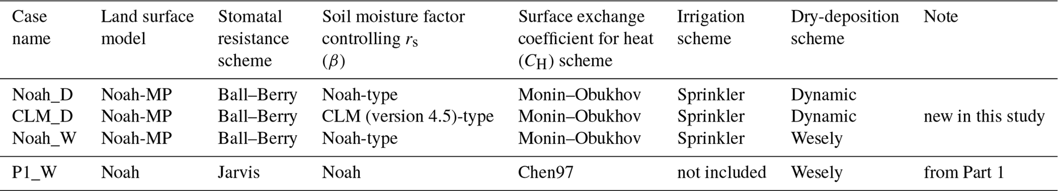
Table 1 Model cases and their configurations relevant to the discussions of this study.

V_max represents the maximum rate of carboxylation, expressed as

$$\begin{array}{}\text{(7)}& V_{\max }=V_{\max \mathrm{25}}{\mathit{\alpha }}_{\mathrm{vmax}}^{\frac{\text{TV}-\mathrm{25}}{\mathrm{10}}}f\left(\mathrm{N}\right)f\left(\text{TV}\right)\mathit{\beta },\end{array}$$

where V_max25 is the maximum carboxylation rate at 25 ^∘C; f(TV) is a function that mimics thermal breakdown of metabolic processes; f(N) is a foliage nitrogen factor; and β is the SM factor controlling r_s, which presents strong dependencies on soil type and hydrological regime. In this study model results based on the Noah and the Community Land Model (CLM; versions 4.5 and earlier) types of β schemes are compared (Table 1), the latter of which is known to often result in sharper and narrower ranges of variation with SM than the former does. The Noah and CLM types of β parameterizations are based on Eqs. (8) and (9), respectively:

$$\begin{array}{}\text{(8)}& {\displaystyle }\mathit{\beta }=\sum _{i=\mathrm{1}}^{N_{\mathrm{root}}}{\displaystyle \frac{\mathrm{\Delta }{z}_i}{z_{\mathrm{root}}}}\min (\mathrm{1.0},{\displaystyle \frac{{\mathit{\theta }}_{\mathrm{liq},i}-{\mathit{\theta }}_{\mathrm{wilt}}}{{\mathit{\theta }}_{\mathrm{ref}}-{\mathit{\theta }}_{\mathrm{wilt}}}})\text{(9)}& {\displaystyle }\mathit{\beta }=\sum _{i=\mathrm{1}}^{N_{\mathrm{root}}}{\displaystyle \frac{\mathrm{\Delta }{z}_i}{z_{\mathrm{root}}}}min\left(\mathrm{1.0},{\displaystyle \frac{{\mathit{\psi }}_{\mathrm{wilt}}-{\mathit{\psi }}_i}{{\mathit{\psi }}_{\mathrm{wilt}}-{\mathit{\psi }}_{\mathrm{sat}}}}\right),\end{array}$$

where

$${\mathit{\psi }}_i={\mathit{\psi }}_{\mathrm{sat}}{\left({\displaystyle \frac{{\mathit{\theta }}_{\mathrm{liq},i}}{{\mathit{\theta }}_{\mathrm{sat}}}}\right)}^{-b}.$$

θ_liq,i, θ_wilt, θ_ref, and θ_sat are SM at soil layer i, wilting point, and reference and saturated SM, respectively. N_root and z_root are the numbers of soil layers containing roots and total depth of the root zone, respectively. ψ_i, ψ_wilt, and ψ_sat are matric potential at soil layer i, and wilting and saturated matric potential, respectively, and b is the Clapp–Hornberger parameter. Major parameters for the calculations of β in both schemes are soil-type-dependent.

Other Noah-MP configurations which can affect the modeled land state and flux variables include the three-layer snowpack physics and the CLASS snow surface albedo; the Jordan scheme for partitioning precipitation into rainfall and snowfall; the Niu-Yang-2006 frozen soil permeability and supercooled liquid water option; the SIMple Groundwater Model runoff scheme; and the Monin–Obukhov C_H scheme, which is based on more general Monin–Obukhov similarity theory and, unlike Noah's default Chen97 (Chen et al., 1997) scheme (Niu et al., 2011; and Sect. S1 of Huang et al., 2021), accounts for the zero-displacement height. Being affected by stability correction and additional effects of planetary boundary layer height on friction velocity, it is likely that the Monin–Obukhov scheme can result in either weaker or greater C_H (i.e., less or more efficient ventilation of the land surface) than the Chen97 scheme during the daytime in summer (Niu et al., 2011; Yang et al., 2011).

The irrigation process was included in all Noah-MP-based simulations in this study. The benefit of including irrigation relies on the choice and parameterization of the irrigation scheme, as well as the LSM's inputs (Lawston et al., 2015). The sprinkler scheme was chosen as it was reported as the prevalent irrigation method in 2015 across the US and many of the states within our model domain (Dieter et al., 2018). Irrigation was triggered over irrigated land in growing season within local morning times (06:00–10:00) when root zone SM drops below 50 % of the soil field capacity. The irrigated land was determined by the model's LULC input and irrigation intensity information in Salmon et al. (2015), and the root zone area was derived from the maximum root depth, which varies by crop type and GVF.

2.3 Wesely and dynamic O₃ dry-deposition schemes

Dry-deposition velocity v_d is estimated based on the resistance analogy approach:

$$\begin{array}{}\text{(10)}& v_{\mathrm{d}}={\displaystyle \frac{\mathrm{1}}{r_{\mathrm{a}}+r_{\mathrm{b}}+r_{\mathrm{c}}}}.\end{array}$$

r_a and r_b are aerodynamic resistance and quasi-laminar sublayer resistance, respectively, sensitive to surface properties such as surface roughness, and follow the Monin–Obukhov similarity theory. Over the land, surface resistance r_c, the major component of v_d, is classified into stomatal–mesophyll resistance (r_s–r_m), cuticular resistance (r_lu), in-canopy resistance (r_dc and r_cl), and ground resistance (r_ac and r_gs):

$$\begin{array}{}\text{(11)}& r_{\mathrm{c}}={\displaystyle \frac{\mathrm{1}}{\frac{\mathrm{1}}{r_{\mathrm{s}}+r_{\mathrm{m}}}+\frac{\mathrm{1}}{r_{\mathrm{lu}}}+\frac{\mathrm{1}}{r_{\mathrm{dc}}+r_{\mathrm{cl}}}+\frac{\mathrm{1}}{r_{\mathrm{ac}}+r_{\mathrm{gs}}}}},\end{array}$$

where r_dc is resistance for gas-phase transfer affected by buoyant convection in the canopy when sunlight heats the (near-)surface, r_cl is resistance for leaves, twigs, bark, and others in the lower canopy, r_ac is resistance for transfer that depends mostly on canopy structure, and r_gs is resistance for soil, leaf litter, snow, and others at the ground surface.

Two deposition schemes, namely the Wesely and a dynamic scheme, were applied in this study, in which r_s and r_lu are treated differently. In the Wesely scheme, r_s and r_lu are calculated based on Eqs. (12) and (13):

$$\begin{array}{}\text{(12)}& {\displaystyle }{r}_{\mathrm{s}}=\left\{\begin{array}{l}{r}_i\left\{\mathrm{1}+{\left[\frac{\mathrm{200}}{G+\mathrm{0.1}}\right]}^{\mathrm{2}}\right\}\left\{\frac{\mathrm{400}}{T_{\mathrm{s}}(\mathrm{40}-T_{\mathrm{s}})}\right\}\frac{D_{{\mathrm{H}}_{\mathrm{2}}\mathrm{O}}}{D_x},\\ \mathrm{0}{}^{\circ }\mathrm{C}\le T_{\mathrm{s}}\le \mathrm{40}{}^{\circ }\mathrm{C}\\ \sim \mathrm{9999},\\ \mathrm{\text{ assuming mass transfer through stomata stops}},\\ T_{\mathrm{s}}>\mathrm{40}{}^{\circ }\mathrm{C}\text{ or}<\mathrm{0}{}^{\circ }\mathrm{C}\end{array}\right.\text{(13)}& {\displaystyle }\begin{array}{rl}& r_{\mathrm{lu}}={\displaystyle \frac{r_{\mathrm{lu},\min }}{{\mathrm{10}}^{-\mathrm{5}}H+f_{\mathrm{0}}}}+\mathrm{1000}{e}^{-T_{\mathrm{s}}-\mathrm{4}},\\ & \text{for dry surfaces according to humidity and precipitation fields},\end{array}\end{array}$$

where the LULC- and season-dependent constants r_i and r_lu,min represent the minimum stomatal and cuticular resistances, respectively, which are subject to uncertainty; G and T_s are radiation and surface temperature, respectively, whose definitions are different than those of PAR and TV in Eqs. (2)–(7); $D_{{\mathrm{H}}_{\mathrm{2}}\mathrm{O}}$ and D_x are molecular diffusivities for water vapor and trace gas x (e.g., O₃), respectively; H, which is sensitive to surface temperature, represents the Henry's law constant for the focused trace gas; and f₀ is a reactivity factor for oxidation. The Wesely-scheme-related results that are new from this study and those from Huang et al. (2021) are compared (Table 1).

As expressed in Eq. (14), in the dynamic scheme, r_s used in dry-deposition modeling was taken from what's calculated from Noah-MP's dynamic vegetation model and thus considers the physiological process of leaf responses to photosynthesis rate, humidity, and CO₂ concentrations. The direct effects of SM, as reflected in the β formula, as well as other environmental variables, are included in this method, and this work quantifies the impact of the β factor configurations in Noah-MP (Table 1) on the dynamic-scheme-related results.

$$\begin{array}{}\text{(14)}& r_{\mathrm{s}}=\left({\displaystyle \frac{r_{\mathrm{s},\mathrm{sunlit}}{L}_{\mathrm{sunlit}}+r_{\mathrm{s},\mathrm{shaded}}{L}_{\mathrm{shaded}}}{\text{LAI}}}\right){\displaystyle \frac{D_{{\mathrm{H}}_{\mathrm{2}}\mathrm{O}}}{D_x}},\end{array}$$

where r_s, sunlit and r_s, shaded are computed based on Eqs. (2)–(7), and L_sunlit and L_shaded are proportional to the sunlit and shaded fractions of canopy, respectively, calculated based on the modified two-stream radiation transfer scheme.

In the dynamic scheme, r_lu for dry surfaces is modified from the Wesely formula by considering its LAI dependency:

$$\begin{array}{}\text{(15)}& r_{\mathrm{lu}}={\displaystyle \frac{r_{\mathrm{lu},\min }}{\text{LAI}\times ({\mathrm{10}}^{-\mathrm{5}}H+f_{\mathrm{0}})}}+\mathrm{1000}{e}^{-T_{\mathrm{s}}-\mathrm{4}}.\end{array}$$

In both the Wesely and the dynamic schemes, r_dc is sensitive to surface radiation, and r_m is expressed as

$$\begin{array}{}\text{(16)}& r_{\mathrm{m}}={\displaystyle \frac{\mathrm{1}}{\frac{H}{\mathrm{3000}}+\mathrm{100}{f}_{\mathrm{0}}}}.\end{array}$$

Similar to the r_lu calculations in Eqs. (13) and (15), to approximate an effect that coldness sometimes reduces the uptake, $\mathrm{1000}{e}^{-T_{\mathrm{s}}-\mathrm{4}}$ is added to LULC- and season-dependent constants to derive r_gs and r_cl. It is worth mentioning that the direct effects of water stress on mesophyll resistance have been recognized (e.g., Egea et al., 2011). Yet, in neither scheme we applied have such effects been incorporated into the r_m formula as part of the v_d calculation.

2.4 Model evaluation, analysis, and O₃ impact assessments

For the cases listed in Table 1, we quantify the impacts of SM DA on the modeled SM, vegetation dynamics, surface fluxes, and meteorological and surface O₃ fields during the 16–28 August 2016 period. The focused surface fluxes are gross primary productivity (GPP), which is integrated by LAI from A in Eqs. (2)–(3), energy fluxes and their partitioning in the format of evaporative fraction (EF = daily latent heat $/$ (daily latent heat + daily sensible heat)), dry-deposition flux and individual v_d terms for O₃, particularly the r_s- and r_lu-related terms. The SM DA impacts on most of these model fields are expressed as daily and/or daytime (around 13:00–24:00 UTC) averaged absolute or relative changes referring to the results from the no-DA cases. For O₃ dry-deposition fluxes, we also conducted linear regression analyses to determine the relationships between the relative flux changes and the relative changes in column-averaged initial SM due to the DA. Results of O₃ dry-deposition fluxes and the regression analyses (i.e., slopes and their standard errors, correlation coefficient r values, and p values) are summarized by grouped LULC types defined in Fig. 1a. Case studies were also conducted at two low-elevation forested sites where we investigated in detail the diurnal and daily variability of O₃ dry-deposition fluxes from various model cases and an independent dataset.

Table 2 Evaluation datasets relevant to this study, along with their key attributes. References of these products can be found in the “Data availability” section of this work and Huang et al. (2021).

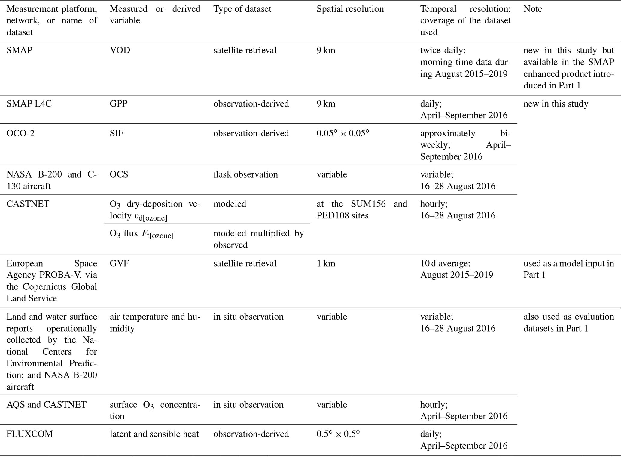
Acronyms: AQS – Air Quality System, CASTNET – Clean Air Status and Trends Network, GPP – gross primary productivity, GVF – green vegetation fraction, L4C – level 4 carbon, OCO-2 – Orbiting Carbon Observatory-2, OCS – carbonyl sulfide, PROBA-V – Project for On-Board Autonomy – Vegetation, SIF – solar-induced chlorophyll fluorescence, SMAP – Soil Moisture Active Passive, and VOD – vegetation optical depth.

A variety of data products were utilized in this study to assess the model performance in no-DA and DA cases (Table 2). Many of these evaluation datasets have been applied and introduced in detail in Huang et al. (2021), which are (1) National Centers for Environmental Prediction Global Surface Observational Weather Data as well as weather data collected on board the NASA B-200 aircraft during the ACT-America campaign; (2) hourly surface O₃ measurements at the US Environmental Protection Agency Clean Air Status and Trends Network (CASTNET) and Air Quality System (AQS) sites; and (3) daily, 0.5^∘ × 0.5^∘ FLUXCOM latent and sensible heat fluxes. New evaluation datasets used in this work include (1) VOD retrievals from the 9 km enhanced SMAP product, which indicates the attenuation of microwave signals by vegetation, proportional to above-ground canopy biomass, and was used together with a 10 d average Copernicus Global Land Service GVF product to derive GVF for the focused 13 d period; (2) daily GPP estimates from the 9 km SMAP level 4 carbon (L4C) product version 6, developed based on the SMAP L4 surface (0–5 cm) and root zone (0–100 cm) SM together with satellite LULC and vegetation datasets; (3) two independent GPP proxies (Whelan et al., 2020) of satellite-derived solar-induced chlorophyll fluorescence (SIF) data (Yu et al., 2019) and the Portable Flask Package (Sweeney et al., 2015) carbonyl sulfide (OCS) measurements collected on board the B-200 and C-130 aircraft during the ACT-America campaign, with the OCS data being analyzed together with other airborne trace gas (e.g., benzene) measurements during this campaign to help distinguish the influences of combustion sources from plant CO₂ uptake on the observed OCS distributions; and (4) v_d data from two selected CASTNET sites, estimated using a multilayer model (MLM; not supported by CASTNET as of 2017) version 3.0, which has known limitations and biases against eddy covariance flux measurements as well as v_d estimated using other methods (e.g., Finkelstein et al., 2000; Saylor et al., 2014; Wu et al., 2018). The known limitations of MLM and how they may affect our model comparisons with the CASTNET v_d data are discussed. Our O₃ dry-deposition results are also compared with eddy covariance measurements reported in independent works for similar climate and/or LULC types during other time periods.

This study also evaluates how the SM DA affected the assessments of surface O₃ impacts on human and ecosystem health. Specifically, (1) MDA8 O₃ fields over urban and nonurban terrestrial regions were investigated linked to their respective population ranges, and (2) the LULC-specific phytotoxic ozone dose above the critical level of y nmol m⁻² s⁻¹ (POD_y) and the crop-specific AOT40, which are defined in Eqs. (17) and (18), were evaluated.

$$\begin{array}{}\text{(17)}& {\text{POD}}_y\left(\mathrm{mmol}{\mathrm{m}}^{-\mathrm{2}}\right)=\sum \left[\left(F_{\mathrm{s}}-y\right)\times {\displaystyle \frac{\mathrm{3600}}{{\mathrm{10}}^{\mathrm{6}}}}\right],\end{array}$$

for hourly daytime stomatal uptake F_s>y nmol m⁻² s⁻¹, and

$$\begin{array}{}\text{(18)}& \mathrm{AOT}\mathrm{40}\left(\mathrm{ppmh}\right)=\sum \left[\right(C-\mathrm{0.04}\left)\right],\end{array}$$

for hourly daytime O₃ concentration C>0.04 ppmv.

According to Convention on Long-Range Transboundary Air Pollution (CLRTAP, 2017), the stomatal O₃ uptake F_s needed in POD_y calculations was derived based on Eq. (19):

$$\begin{array}{}\text{(19)}& F_{\mathrm{s}}=C\left(\mathrm{nmol}{\mathrm{m}}^{-\mathrm{3}}\right)\times g_{\mathrm{s}}\times {\displaystyle \frac{r_{\mathrm{c}}}{\mathrm{1.3}\times \mathrm{150}\times \sqrt{\frac{L}{u}}+r_{\mathrm{c}}}},\end{array}$$

where g_s, L, and u are stomatal conductance, leaf width (0.04 m in this work), and surface wind speed, respectively.

The calculated POD_y and AOT40 were used to estimate the relative biomass loss (RBL) or relative yield loss (RYL) for several types of vegetation or crops based on dose–response functions reported in literature (Table 3, CLRTAP, 2017; Mills et al., 2007, 2018b). Our 13 d WRF-Chem model results were linearly extrapolated to approximately 3 months to derive the POD_y and AOT40 fields. While we assess the uncertainty due to such linear extrapolations by relating our 13 d/extrapolated surface O₃ and flux results to seasonal (e.g., averaged for 3 consecutive months) conditions in 2016, we focus on qualitatively interpreting the results and discussing their implications. The outcome from this analysis is also compared with the findings from several independent O₃ impact assessment studies for different time periods.

Table 3 Dose–response functions used to estimate the LULC- and crop-specific relative yield losses (i.e., 1 – relative yield, RY) due to O₃ exposure and uptake, along with their references.

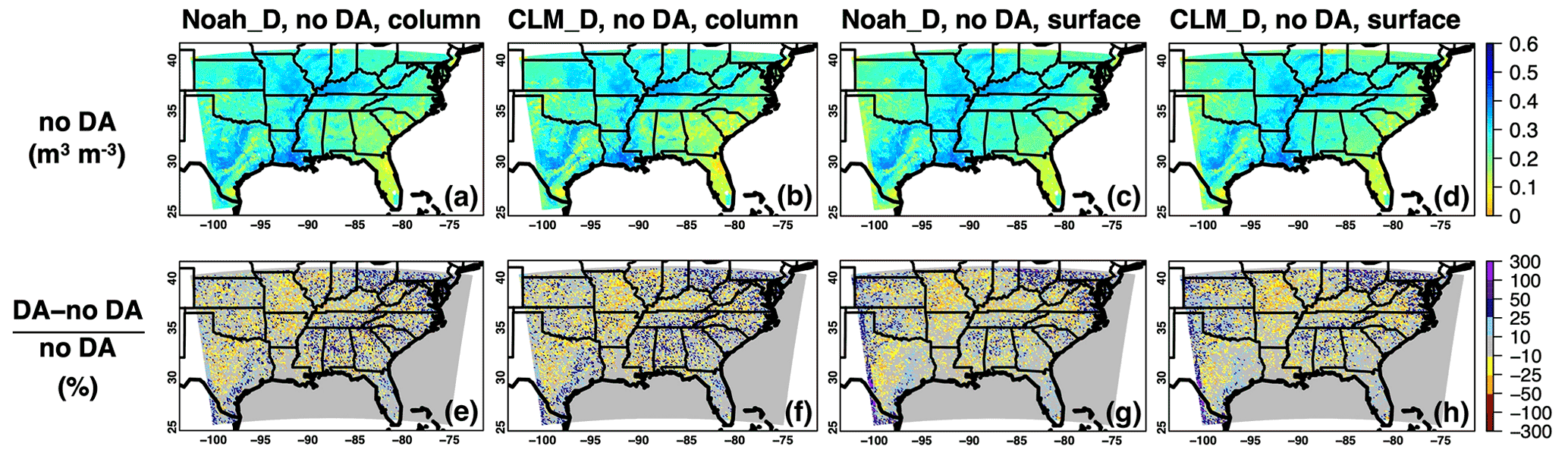
Figure 2 Period-mean (16–28 August 2016) WRF-Chem (a, b) column-averaged and (c, d) surface-layer soil moisture fields at initial times and (e–h) their relative changes in percent due to the SMAP DA. Results based on the Noah_D and CLM_D cases are shown in (a), (c), (e), and (g) and (b), (d), (f), and (h), respectively.

3 Results and discussions

3.1 Modeled SM and vegetation fields

Figure 2 compares the horizontal and vertical gradients of the model's initial SM conditions from the Noah_D and CLM_D cases defined in Table 1, in which the Noah and CLM types of β factor schemes were applied. At the surface layer (0–10 cm belowground), both cases produced SM horizontal gradients that resemble the Noah-based results presented in Huang et al. (2021). They are moderately correlated with the column-averaged SM fields (r=0.875 and 0.871, respectively), and the mean differences in column-averaged and surface SM from the Noah_D and CLM_D cases are 0.003 and −0.006 m³ m⁻³, respectively. Kumar et al. (2009) have found that, compared to other LSMs such as the Catchment model (based on which the SMAP L4 datasets are produced), the 4-soil-layer Noah and 10-soil-layer CLM LSMs display successively weaker surface–subsurface coupling strengths, and the weakest coupling strength of CLM was primarily attributed to its significantly larger number of soil layers. The slightly weaker surface–subsurface correlations in the CLM_D case than in the Noah_D from this work, both based on a 4-soil-layer Noah-MP modeling system, indicate the minor role of the LSM physics, in particular the β factor scheme, in controlling the vertical coupling strength of SM conditions.

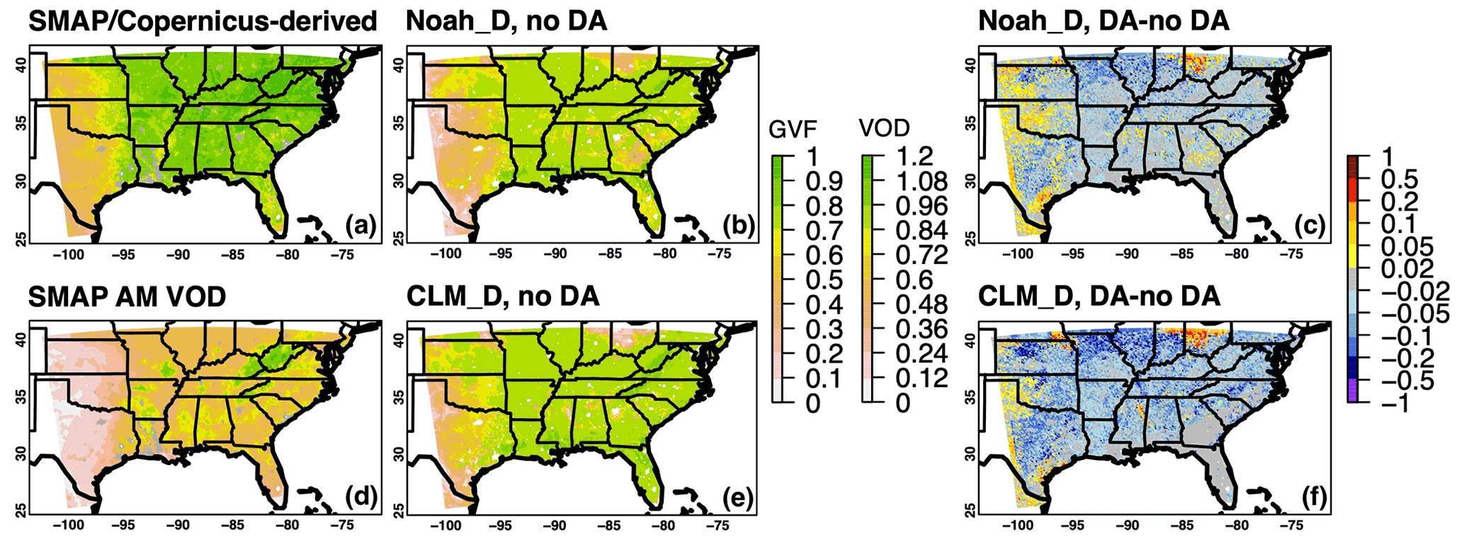
Figure 3 Period-mean (16–28 August 2016) green vegetation fraction (GVF) (a) derived from the Copernicus Global Land Service product and the SMAP morning-time (AM) vegetation optical depth (VOD) using the method described in Fig. S2 and (b, c, e, f) based on WRF-Chem calculations as well as their responses to the SMAP DA. The GVF results from the Noah_D and CLM_D cases are shown in (b) and (c) and (e) and (f), respectively. Period-mean SMAP AM VOD is shown in (d). In (a) and (d), grey indicates missing data over terrestrial regions.

The modeled SM fields from the Noah_D and CLM_D differ on grid scale, particularly in the subsurface zones (Fig. 2a and b). For example, in sand-dominant regions that were experiencing drought conditions during this period (e.g., Florida and the Texas–Oklahoma border regions, where simulated SM is mostly under 0.2 m³ m⁻³), column-averaged SM values from the CLM_D case are notably smaller than those from the Noah_D case. These results contrast with those reported by Niu et al. (2011), in which cases using Noah-MP with the CLM-type β factor led to less soil water consumption and thus smaller SM variability during drought periods than using it with the Noah-type β factor. In their cases focusing on loam and clay soil that have higher wilting points when the CLM-type β factor scheme was applied, plant transpiration ceased to save soil water under drought conditions. Our results can be explained by the steeper CLM-type β–SM curve than the Noah-type β–SM curve for low SM, sand-dominant areas, as illustrated in Fig. 3a of Niu et al. (2011). For such conditions, Noah-MP with the CLM-type β factor produces stronger evapotranspiration (ET) and consumes more soil water, resulting in drier soil. For wet regions where SM values exceed 0.4 m³ m⁻³, such as Louisiana and Arkansas, the CLM- and Noah-type β values are close to 1.0 and insensitive to soil type and SM variations; therefore, SM and ET produced from the Noah_D and CLM_D cases do not diverge. These findings corroborate the conclusions by Yang et al. (2011) that the degree of the β impacts on the SM–ET relationship should depend on the soil type and hydrological regime, and they are important for understanding the vegetation and surface flux results to be presented in the later parts of this paper.

Referring to the SMAP SM data, in general, surface SM produced by the no-DA modeling systems shows wet biases in non-forested regions and dry biases over the forests for the study period. These SMAP–model discrepancies were successfully reduced by the DA for all vegetated LULC groups (Fig. S1, left), leading to overall slightly drier soil in DA-enabled simulations. For both the Noah_D and CLM_D cases, the DA adjusted the modeled SM fields across the entire soil columns, demonstrating that observational information at the surface was propagated into deep soil layers. The SM responses to the DA as a function of soil layer from the Noah_D and CLM_D cases are roughly similar but different at small spatial scales, which reflect the controls of the β factor scheme on the surface–subsurface coupling strengths of the modeling/DA system used. With the SMAP DA enabled, the r values between column-averaged and surface SM from the Noah_D and CLM_D cases increased to 0.902 and 0.897, respectively.

The satellite-derived GVF fields (methods introduced in Fig. S2 caption) transition from low to moderate (<0.6) to high (>0.8) values from the western (mostly shrub/grasslands) to the central and eastern parts (forests- and croplands-dominant) of the study region, and such spatial gradients are highly correlated with the SMAP VOD retrievals (Fig. 3a and d). The Noah_D and CLM_D cases both reproduced these spatial patterns moderately well. Major differences between these cases are found in dry sandy regions, where, as discussed in previous paragraphs, more soil water was consumed for ET and plant growth in the CLM_D case and therefore higher GVF values are given. Overall, the DA adjustments to the modeled GVF and SM fields are positively correlated (Fig. S1, right), and the relative changes in GVF are smaller. While the SM changes in the Noah_D and CLM_D cases are of close magnitude, GVF responded more strongly in the CLM_D case except for sandy regions. Referring to the satellite-derived GVF fields which are also subject to large uncertainty (as discussed in Fig. S2 caption), the modeled vegetation fields are more effectively improved by the DA over sparsely vegetated regions such as the South Central Plains. The DA also remarkably reduced the model–satellite mismatches over some of the dense vegetation regions such as southwestern Ohio. The likely degraded model performance over certain dense vegetation areas can be partially explained by weaknesses related to the SM–vegetation growth feedbacks (more details in Fig. S1 caption) in the dynamic vegetation model parameterizations which need to be identified and addressed in future work. It is also suggested that joint assimilation of satellite SM and vegetation phenology products such as the VOD retrievals needs to be attempted, which may maximize the positive DA impacts on multiple land variables and their atmospheric feedbacks.

Table 4 Evaluation of daily-averaged WRF-Chem gross primary productivity and evaporative fraction, referring to the SMAP L4C and FLUXCOM datasets.

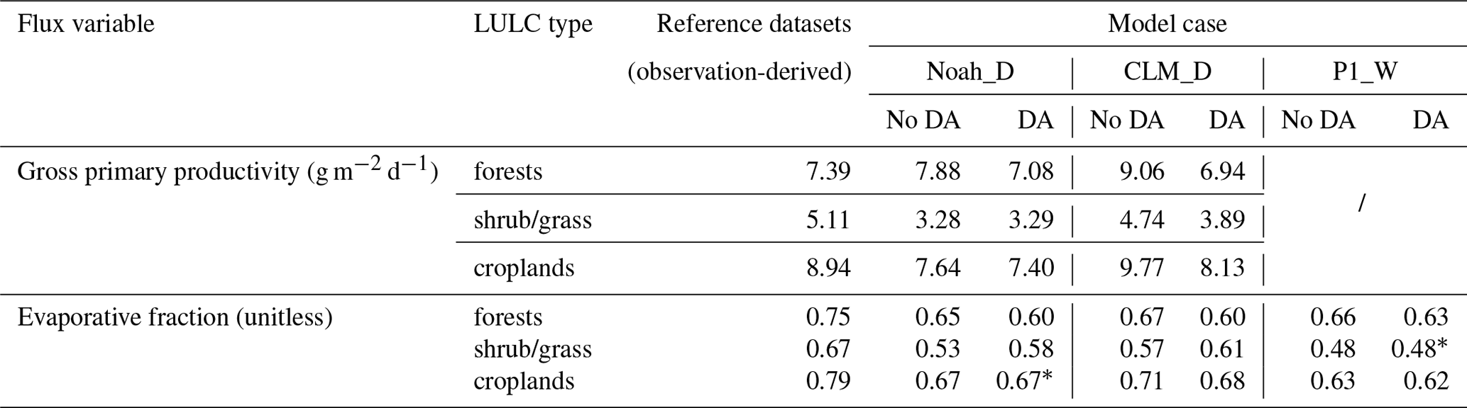
^∗ The increases from no-DA cases, which led to improved model performance, are <0.005.

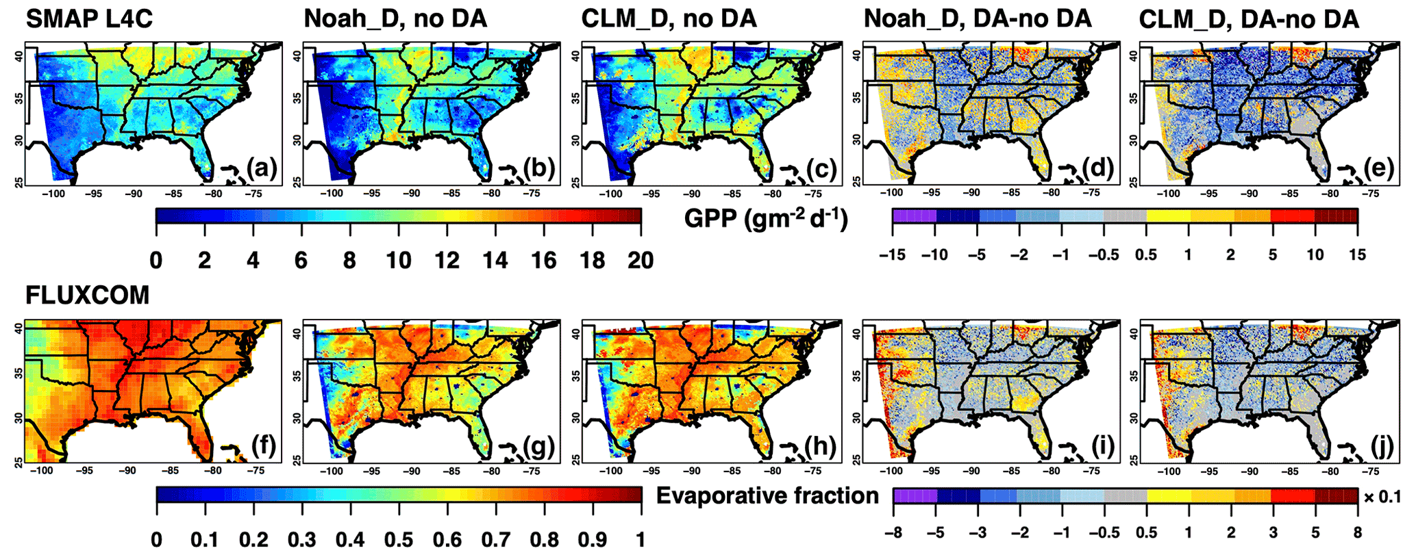
Figure 4 Period-mean (16–28 August 2016) WRF-Chem calculated (b–e) gross primary productivity (GPP) and (g–j) evaporative fraction as well as their responses to the SMAP DA. Results based on the Noah_D and CLM_D cases are shown in (b), (d), (g), and (i) and (c), (e), (h), and (j), respectively. Period-mean SMAP L4C GPP and FLUXCOM evaporative fractions are shown in (a) and (f), respectively, which are also used to evaluate the model results (Table 4).

3.2 Modeled fluxes and weather conditions

3.2.1 Carbon/energy fluxes and weather conditions

Figure 4 compares the spatial distributions of the period-mean WRF-Chem carbon and energy fluxes with SMAP L4C and FLUXCOM products which contain observation information, and Table 4 summarizes WRF-Chem and observation-derived flux results by three LULC groups. The observation-derived products indicate the highest GPP and EF over croplands. Without the DA, the Noah-MP-related cases outperformed the Noah-related P1_W case on simulating EF, especially over shrub/grassland and cropland regions. This indicates that, from Noah to Noah-MP, the multiple updates in LSM physics related to r_s, irrigation, and C_H are beneficial. Larger GPP and EF values are found in CLM_D than in Noah_D; most of these larger values match better with the SMAP L4C and FLUXCOM data. The DA led to increased EF over shrub/grasslands in all model cases as well as over croplands in the Noah_D case, bringing the model results closer to the FLUXCOM data. The EF values were unfavorably reduced by the DA in the CLM_D and P1_W cases over croplands and in all model cases over forests, reflecting the challenges of satellite SM DA over regions with dense vegetation and/or affected by human activities, which have also been reported and discussed in previous studies (e.g., Huang et al., 2021). For the Noah_D and CLM_D cases, this may also be due to the possibly degraded vegetation performance discussed in Sect. 3.1. The modeled GPP in the CLM_D cases was lowered by the DA overall, which helped reduce the model–SMAP L4C discrepancies over forests and croplands. In the Noah_D case, GPP was improved by the DA over forests and (slightly) over shrub/grasslands. Based on the evaluation statistics, for this case, the CLM-type β factor scheme is shown to be slightly superior to the Noah type. Note that the quality of the SMAP L4C and FLUXCOM products may also be strongly LULC-dependent; e.g., it has been known that the uncertainty of SMAP L4C data is generally larger for highly productive plant functional types (Kimball et al., 2021). Such evaluation, therefore, has demonstrated the critical role of LULC type in understanding the model performance of carbon and energy fluxes and its responses to satellite SM DA.

Additional datasets were also utilized to help understand terrestrial carbon uptake, including satellite SIF and ACT-America aircraft OCS, as well as its vertical gradients (Fig. S3). Consistent with the SMAP L4C- and WRF-Chem-based results, the largest SIF values are shown over croplands, especially maize and soybean fields in Illinois and Indiana, 2–3 times as high as those over shrub/grasslands in the South Central Plains. All these datasets suggest moderate to high terrestrial carbon uptake around the Lower Mississippi croplands and the forests and croplands near the Texas–Oklahoma border, which is supported by the large OCS drawdowns (i.e., the free tropospheric-near surface gradients far exceeded 60 pptv) along with other trace gas measurements taken on board the B-200 and C-130 aircraft.

Figure 5 Period-mean (16–28 August 2016) WRF-Chem calculated daytime (a–c) surface air temperature and (g–i) surface radiation as well as (d–f, j–l) their responses to the SMAP DA. Results based on the Noah_D, CLM_D, and P1_W cases are shown in (a), (d), (g), and (j), (b), (e), (h), and (k), and (c), (f), (i), and (l), respectively. Overall, the weather fields from Noah_D and Noah_W (not shown in figures) cases are nearly the same. Grey lines in (a) indicate the B-200 flight paths over the southeastern US during the 2016 ACT-America campaign.

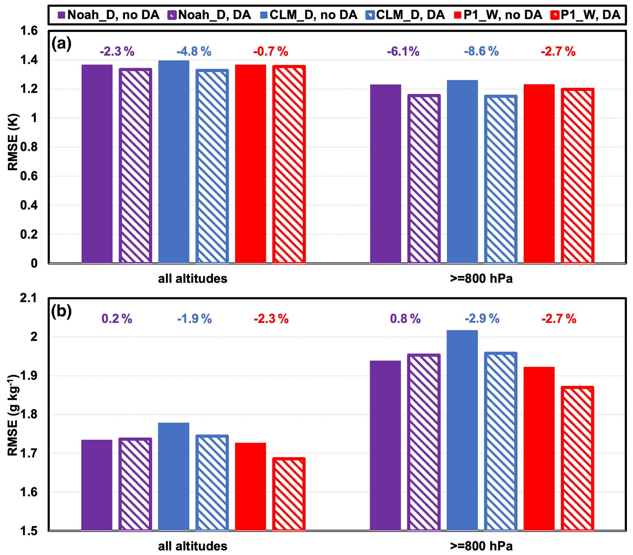
Figure 6 Evaluation of (a) air temperature and (b) water vapor mixing ratios from several WRF-Chem simulations with the B-200 aircraft observations during the 2016 ACT-America campaign. The RMSEs are summarized in barplots based on model comparisons against observations at all altitudes and near the surface (i.e., ≥800 hPa). Colored texts above the barplots indicate the SMAP DA impacts on RMSEs. The B-200 flight paths are indicated in Fig. 5a.

In general, the modeled EF fields as well as their directions of changes due to the DA resemble those of latent heat flux and relative humidity (RH), which are opposite to those of sensible heat and surface temperatures (Figs. 5 and S4). The model reproduced the observed spatiotemporal variability of 2 m air temperature (T2) and RH, as well as FLUXCOM latent and sensible heat fluxes, well overall. The diagnostic 2 m weather fields and their responses to the DA strongly correlate with the model's surface-level results. The Noah-MP-related cases reacted more strongly to the DA than the Noah-related cases, with the responses in the CLM_D case larger than in the Noah_D case except for dry, sandy regions, which can be attributed to combined effects of the C_H and stomatal resistance schemes used. It is important to note that diagnostic temperature and humidity variables are represented differently in Noah and Noah-MP and thus are not directly comparable. Specifically, in Noah, T2 is an explicit function of surface temperature, air density, specific heat of dry air at constant pressure, and 2 m surface exchange coefficient for heat, and 2 m specific humidity is a function of surface specific humidity, upward moisture flux at the surface, air density, and 2 m surface exchange coefficient for moisture, whereas in Noah-MP, they are expressed as functions of temperatures and water vapor for vegetated land and bare soil being weighted by their respective fractions. We therefore focus on quantitatively evaluating and intercomparing prognostic model weather variables (i.e., the model-level air temperature and humidity) against ACT-America aircraft observations (Fig. 6). For air temperature, at all altitudes and near the surface (i.e., ≥800 hPa), the CLM_D case responded most strongly to the DA, and the DA-enabled CLM_D case outperformed the Noah_D and P1_W cases. This performance is qualitatively consistent with the model's sensible heat performance referring to the FLUXCOM data. As for humidity, despite the most significant DA improvements in CLM_D, the Noah-MP-related cases did not perform as well as the Noah-related cases, which is also found in the model's latent heat performance in comparison with the FLUXCOM data. However, note that the model's humidity performance is more strongly related to that of r_s and v_d in the Noah-MP-based cases via the direct impacts of humidity on r_s calculations (Eq. 2). The solar radiation fields from all model cases, which play vital roles in controlling the land–atmosphere exchanges of water and trace gases, do not differ remarkably, and their responses to the DA are negligible (e.g., Fig. 5g–l). This indicates that the DA impacts on the modeled surface fluxes resulted primarily from the changes in the modeled SM, humidity, and canopy and/or surface temperatures, as well as vegetation fields. In many cases, these primary contributing factors to the DA impacts are interdependent, and their relative contributions vary by location and time.

Table 5 The 24 h and daytime mean O₃ deposition velocity (v_d[ozone]) and flux (F_t[ozone]) for three LULC groups, from various model cases.

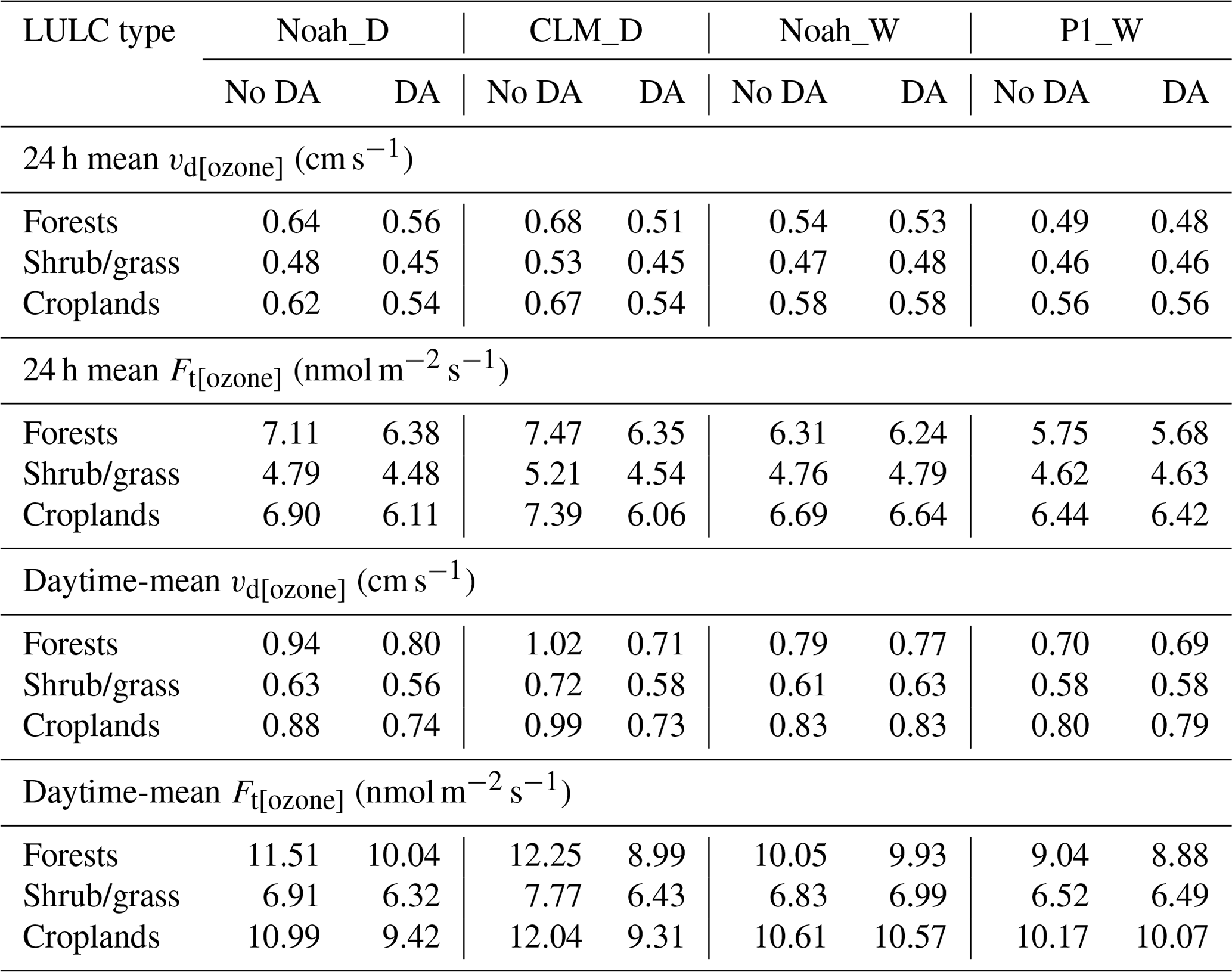
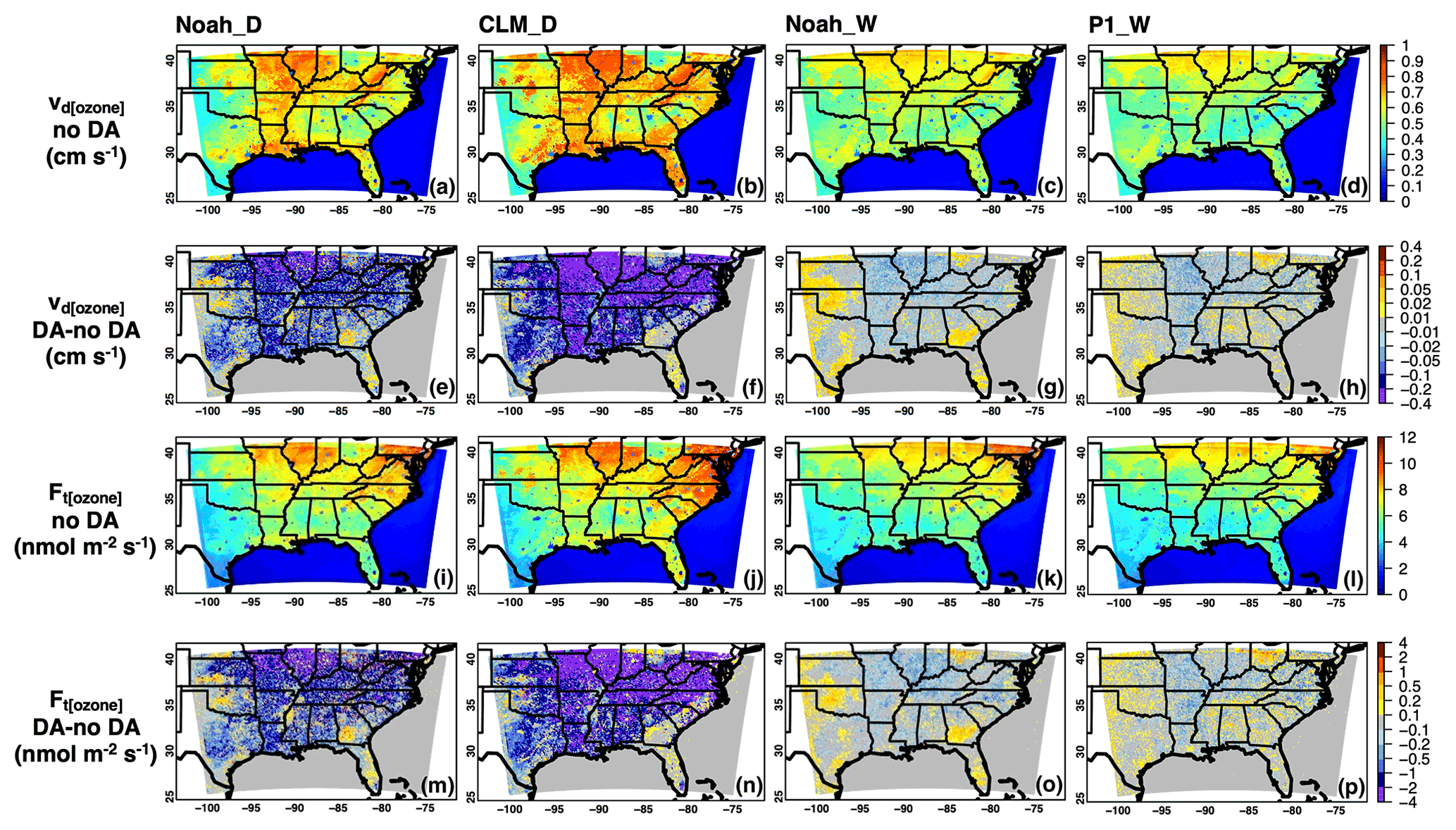
Figure 7 Period-mean (16–28 August 2016) WRF-Chem (a–d) O₃ dry-deposition velocity and (i–l) O₃ dry-deposition flux, as well as (e–h, m–p) the impacts of SMAP DA on these model fields. Results are shown for (a, e, i, m) Noah_D, (b, f, j, n) CLM_D, (c, g, k, o) Noah_W, and (d, h, l, p) P1_W cases, averaged throughout the day.

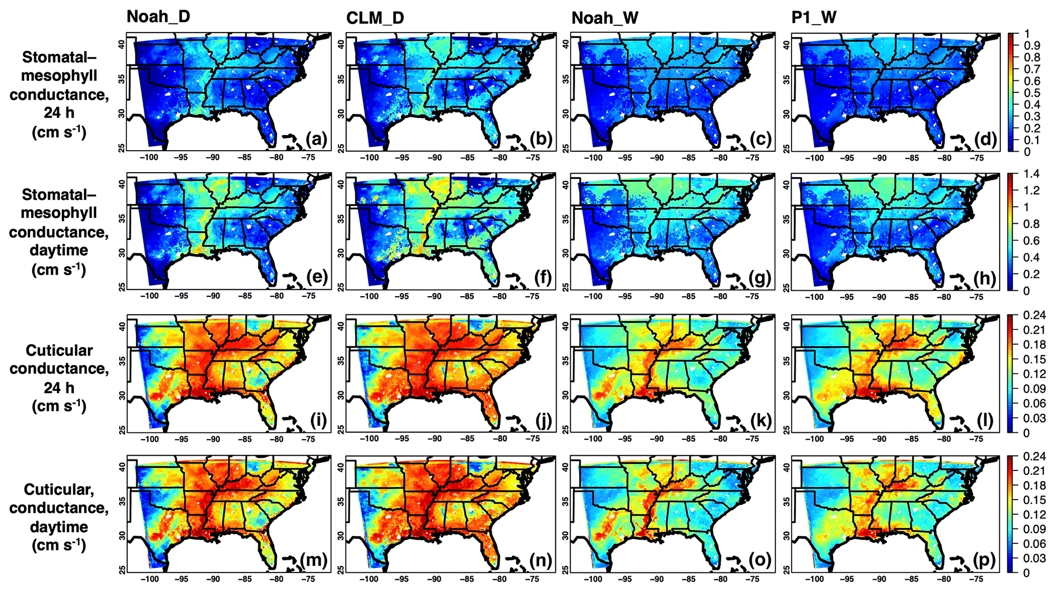
Figure 8 Period-mean (16–28 August 2016) WRF-Chem (a–h) stomatal–mesophyll and (i–p) cuticular conductances over terrestrial regions that do not belong to the urban category in Fig. 1a. Results are shown for (a, e, i, m) Noah_D, (b, f, j, n) CLM_D, (c, g, k, o) Noah_W, and (d, h, l, p) P1_W no-DA cases, averaged (a–d, i–l) throughout the day and (e–h, m–p) during the daytime.

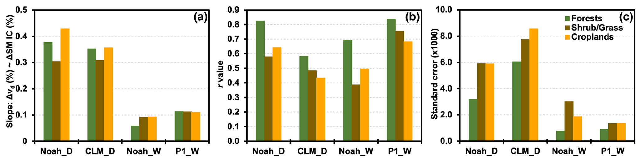
Figure 9 (a) Regression slopes of the relative changes of O₃ dry-deposition velocity v_d versus the relative changes of column-averaged soil moisture initial conditions (SM ICs) due to the SMAP DA, summarized by three LULC groups for all model cases listed in Table 1. The r values of these regression analyses and the standard errors of slopes (%, scaled by 1000) are indicated in (b) and (c), respectively. The p values for all regression analyses are ≪0.01. Regression results for the relative changes of O₃ deposition flux versus the relative changes of SM ICs are similar (not shown in figures).

3.2.2 Ozone dry-deposition velocities and fluxes

Figure 7 presents the period-mean, daily-averaged v_d and dry-deposition flux F_t (i.e., v_d multiplied by concentration at the surface level, Wesely, 1989) for O₃ from all model cases, along with their responses to the SMAP DA. The daytime averages of these fields have similar spatial gradients but of larger magnitudes (not shown in figures). Table 5 summarizes for three LULC groups the daily- and daytime-averaged results. The modeled stomatal–mesophyll and cuticular conductances, as well as their diurnal variability, are indicated in Fig. 8. All model cases produced lower v_d and F_t values over shrub/grasslands than over forests and croplands, qualitatively consistent with results from many existing model- and measurement-based studies (e.g., Val Martin et al., 2014; Hardacre et al., 2015; Silva and Heald, 2018; Lin et al., 2019). The results from Noah_W and P1_W, both of which are based on the same scheme (Wesely), are generally similar, with minor differences largely attributed to different surface temperature fields (Figs. 5 and S4). The WRF-Chem-modeled v_d and F_t fluxes were more strongly affected by the upgrade from the Wesely to the dynamic scheme; i.e., with the updated scheme, they show enhanced magnitudes, stronger spatial variability, and more intensive responses to the DA, especially over forests and croplands. These results can be mainly explained by the fact that the stomatal–mesophyll and cuticular resistances in the dynamic scheme are sensitive to more environmental and biophysical variables, accounting for both the direct and indirect (i.e., via influencing the weather fields and plants' physiology) effects of SM on v_d. v_d from the Noah_D and CLM_D cases, as well as its major term stomatal–mesophyll conductance, shows strong correlations with the modeled GPP, latent heat, and EF fields, which have been discussed in earlier sections. Comparing the cases that implemented the CLM- and Noah-type β schemes, O₃-related fluxes resulting from the former configuration are of notably larger magnitude, spatial variability, and absolute changes due to the DA. The SM impacts on the modeled v_d and F_t were further quantified using linear regression analyses between the relative changes in the modeled O₃ fluxes due to the DA versus those in column-averaged SM initial conditions. All regression models yielded low p values (i.e., ≪0.01), suggesting good Δv_d–ΔSM and ΔF_t–ΔSM relationships. The regression slopes, all with standard errors of <0.01 %, are summarized in barplots (Fig. 9) by three LULC groups for all model cases in Table 1. For all LULC groups, the slopes based on the two cases that implemented the dynamic scheme are 2–3 times larger than those from the two cases using the Wesely scheme, and the slopes differ most strongly among the cases over forests and croplands. The low r values (<0.5) associated with several regression models reflect the stronger nonlinear relationships between the changes in the studied O₃ fluxes and SM. These results emphasize the importance of better understanding and representing in models the SM control on plants' stomatal behaviors which regulate the land–atmosphere exchanges of water, energy, and trace gases. The earlier evaluation of the period-mean GPP and EF across the domain has demonstrated some advantages of using the CLM-type β scheme and that the DA more effectively improved the model performance in sparsely vegetated shrub/grassland regions. These conclusions are likely also applicable to the modeled O₃ dry-deposition process, particularly its stomatal–mesophyll pathway.

In all no-DA and DA cases, the diurnal variability of O₃-related surface fluxes shows clear LULC dependency. Over the shrub/grassland and forests/croplands regions, the daytime-averaged v_d values are 24 %–31 % and 35 %–50 % higher than the 24 h mean, respectively, while the daytime-averaged F_t results are 40 %–50 % and 42 %–63 % higher than the 24 h mean, respectively (Table 5). Such v_d diurnal cycles are a result of the strongest diurnal variability in stomatal–mesophyll conductance (i.e., its daytime mean values are approximately twice as high as the 24 h mean for all LULC types) being balanced out by weak diurnal variability associated with other v_d terms. As the most diurnally variable v_d component, stomatal–mesophyll conductance, on average, contributes less substantially to v_d for shrub/grassland areas (24 h/daytime: up to ∼30 %/40 %) than for forests/croplands (24 h/daytime: up to ∼50 %/66 %), which helps explain the weaker diurnal variability in the modeled v_d over shrub/grasslands. The stronger diurnal cycles in F_t than in v_d reflect the impacts of higher daytime O₃ surface concentrations used in the F_t calculations. The DA did not dominantly intensify or dampen the diurnal cycles of these fluxes for any given grouped LULC type. Whether the DA improved the estimated diurnal cycles of fluxes for various LULC types remains to be evaluated, which can benefit from independent observation-constrained flux products of broad spatial coverage and subdaily variability.

Table 6 Period-mean (16–28 August 2016) soil moisture and surface fluxes at two CASTNET sites shown in Fig. 1d. Standard deviations calculated based on the hourly O₃ dry-deposition velocity v_d[ozone] and flux F_t[ozone] results are also included. Daytime is defined as approximately 08:00–19:00 local standard time.

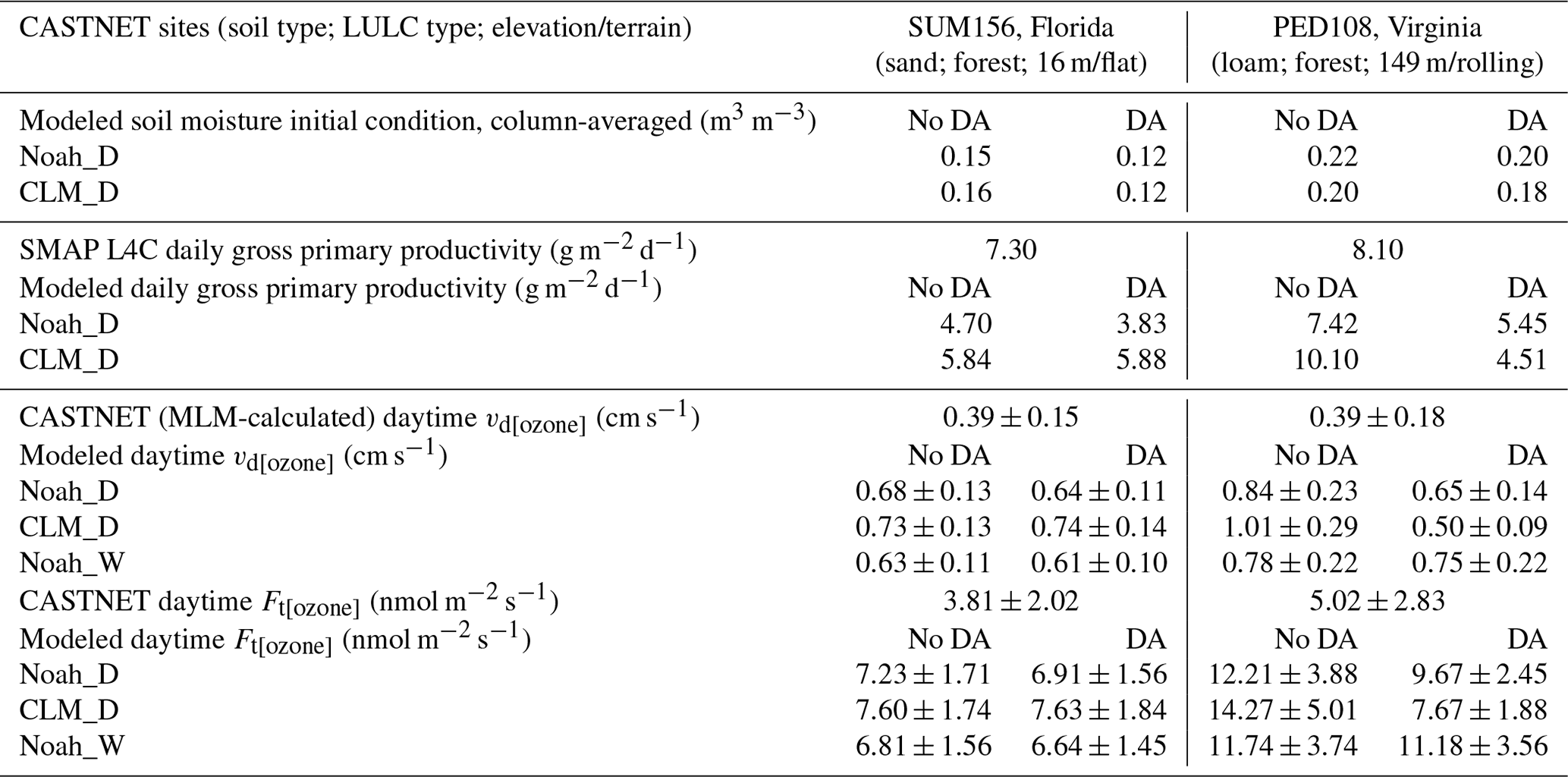
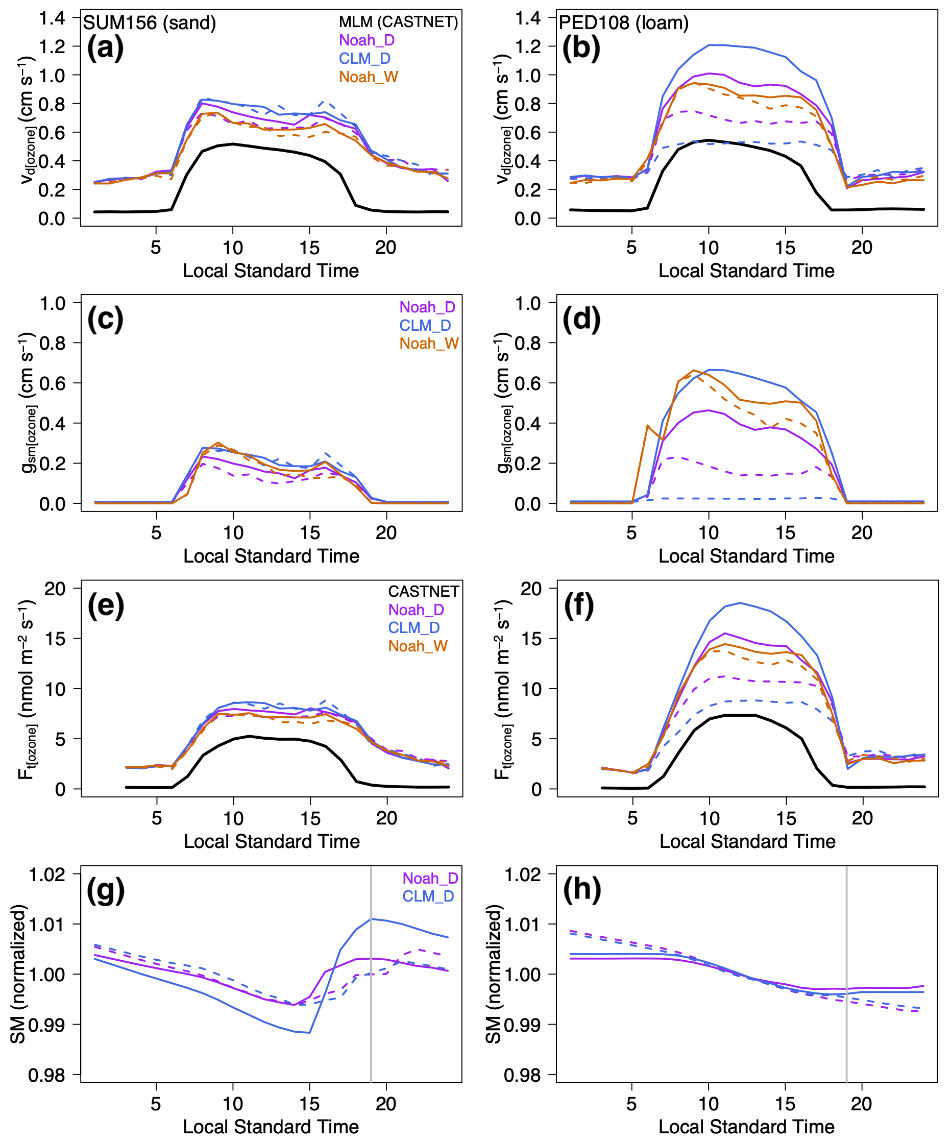
Figure 10 Period-mean (16–28 August 2016) diurnal cycles of (a, b) O₃ dry-deposition velocity v_d and (e, f) O₃ dry-deposition flux F_t based on the CASTNET dataset (shown by solid black lines) and their WRF-Chem counterparts (purple, blue, and brown lines) at the (a, c, e, g) SUM156 and (b, d, f, h) PED108 sites, whose locations are shown in Fig. 1d. Panels (c) and (d) and (g) and (h) indicate the diurnal variability of WRF-Chem stomatal–mesophyll conductance g_sm and column-averaged soil moisture (normalized) at these two sites, respectively. The grey vertical lines in (g) and (h) denote the initial times of WRF-Chem. WRF-Chem results from the no-DA and DA cases are indicated by solid and dashed lines, respectively. Additional time series plots indicating the daily variability of these fluxes are shown in Fig. S5.

A detailed analysis was then conducted at two forest CASTNET sites with different soil types and hydrological regimes. The modeled v_d and F_t from various cases are compared with the operational MLM-based calculations produced at a Florida site SUM156 and a Virginia site PED108 (Figs. 10a, b, e, f and S5; Table 6), where many, most, or all MLM assumptions apply. The dominant soil types at these sites are sand and loam, and the column-averaged SM values from various model cases are approximately 0.15 and 0.20 m³ m⁻³, respectively. These various datasets show that stomatal–mesophyll conductance, v_d, and F_t sharply increase soon after sunrise, reaching their daily maxima in the late morning or early afternoon. The slight declines in fluxes around midday based on some simulations can result from the water and heat stresses which cause stomata closures (Fig. 10c and d). The water stress starts to get relieved from the mid-afternoon at the SUM156 site under the influences of convective precipitation, whereas it persists throughout the afternoon at the PED108 site (Fig. 10g and h). This helps shape the slightly different afternoon flux dynamics at these two locations. Without the DA, at both sites, the highest daytime fluxes were produced from the CLM_D case, followed by the Noah_D and Noah_W cases, which are 2–3 times as high as the MLM-estimated cases. The fluxes from all WRF-Chem cases during the nighttime are close, up to >80 % lower than their daytime maxima, contributed mostly by r_a, r_b, and non-stomatal r_c pathways as stomatal–mesophyll conductance is shown to be negligible (Fig. 10c and d). Despite the uncertainty possibly introduced by the limitations of the Monin–Obukhov similarity theory, our nighttime v_d results are close to flux observations at European forest sites during both dry and wet periods in the past decades (Lin et al., 2020). They are, however, dramatically higher than the MLM-based results that are nearly zero. Wu et al. (2018) compared v_d observations with single-point model calculations based on the operational MLM, Wesely, and Noah-Gas Exchange Model photosynthesis-based scheme, at a Canadian mixed forest site dominated by sand-like soil. Their diverse model results are qualitatively consistent with our findings at the SUM156 and PED108 sites. The remarkably lower v_d values from the operational MLM calculations can be partially attributed to the MLM's simplified approaches of calculating r_a and r_b using wind speed and direction, as well as the empirical approach of calculating r_s which is subject to errors in the season- and LULC-dependent r_i. The possible uncertainty in MLM v_d can also be explained by the lack of continuous, accurate model input data. Specifically, the factual data such as plant and canopy attributes used in the MLM calculations are outdated, which, according to the CASTNET database, represent the conditions in the 2000s; and based on the little day-by-day variability found in the MLM v_d data during the study period which contrasts with our WRF-Chem results (Fig. S5), it is likely that many but not all of these are filled historical average v_d values due to the lack of meteorological measurements that are needed in the MLM calculation. Additionally, based on the surface heterogeneity within the WRF-Chem grids that these sites fall in, representation errors are estimated to be pronounced when comparing the point-scale MLM fluxes with our 12 km WRF-Chem results.

Within the respective ranges of the modeled SM at these two sites, β factors based on the CLM-type scheme are both larger than those based on the Noah-type β scheme (referring to Niu et al., 2011, Fig. 3), which helps explain the higher and more variable model fluxes from the CLM_D case than the Noah_D case without the DA. At SUM156, despite the strongest SM decrease (∼0.04 m³ m⁻³) by the DA in case CLM_D, the modeled fluxes responded least strongly to the DA, in part due to the flattened CLM-type SM–β curves in contrast to the linear Noah-type SM–β function for sand within the 0.12–0.16 m³ m⁻³ SM range. At PED108, the modeled SM values from all model cases were lowered by the DA by ∼0.02 m³ m⁻³. The stronger reactions of fluxes (i.e., v_d, F_t, and their stomatal–mesophyll portions) to the DA from the CLM_D case than those from the Noah_D case can be partially explained by the steep CLM-type SM–β curve versus the linear Noah-type SM–β relationship for loam within the 0.18–0.22 m³ m⁻³ SM range. Our case studies at these two sites with the same type of LULC emphasize the importance of soil type and hydrological regimes for understanding SM controls on dry deposition, which was often omitted or discussed little in previous dry-deposition studies. It is noted that the effectiveness of SM DA in improving the accuracy of land surface states and fluxes at point scale is dependent on the representativeness of the assimilated satellite SM data for these sites, which is expected to increase with the resolutions of the model and the assimilated satellite land product.

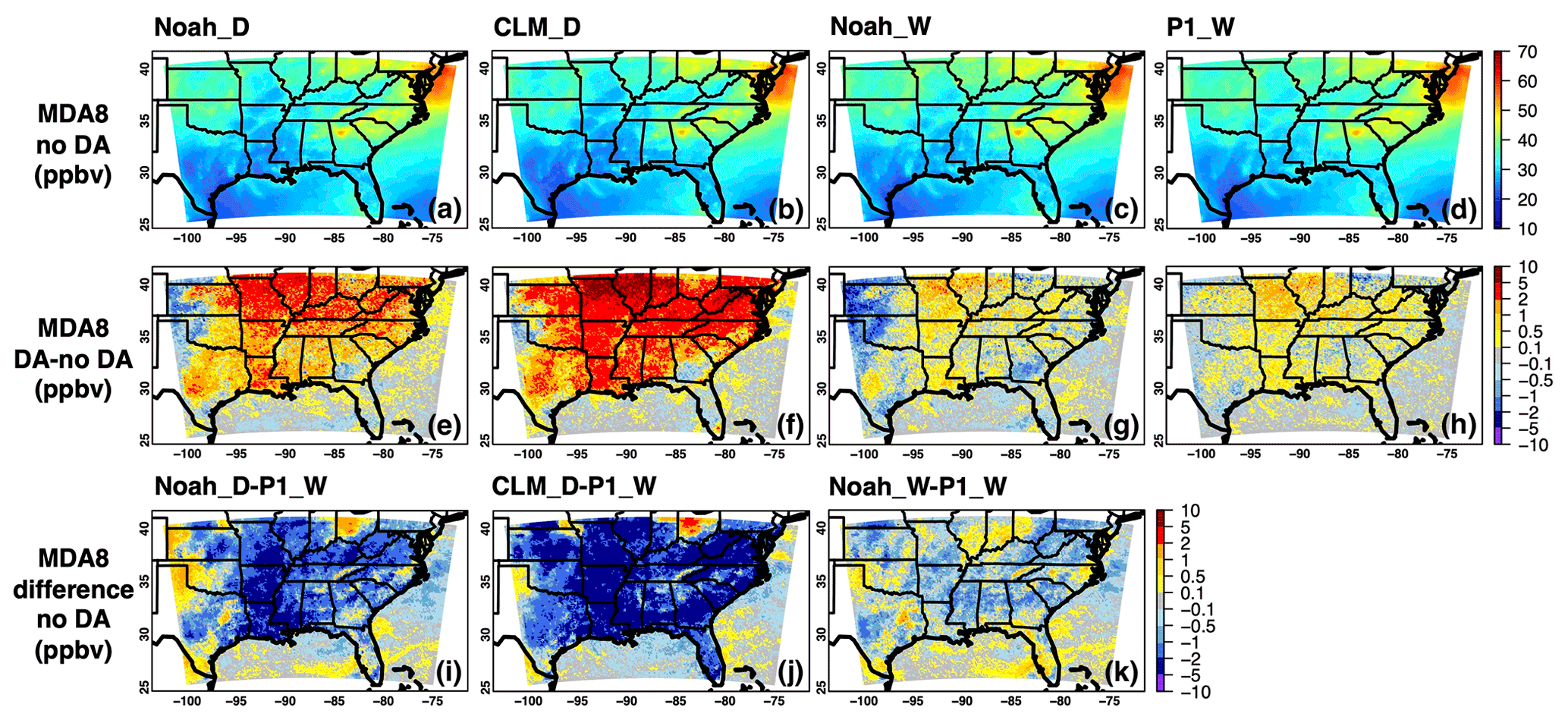
Figure 11 Period-mean (16–28 August 2016) WRF-Chem (a–d) surface MDA8 O₃ fields and (e–h) their responses to the SMAP DA. Results based on the Noah_D, CLM_D, Noah_W, and P1_W cases are shown in (a) and (e), (b) and (f), (c) and (g), and (d) and (h), respectively, and the differences between the Noah-MP-related cases and the P1_W case are shown in (i)–(k).

3.3 Policy-relevant O₃ metrics and implications for O₃ impact assessments

3.3.1 MDA8 and implications for O₃ health impacts

Figure 11 illustrates the impacts of the choice of dry-deposition scheme and SM DA on WRF-Chem-modeled surface MDA8 O₃. During the study period, several warmer- and drier-than-normal Atlantic states experienced high MDA8 at times (i.e., ≥60 ppbv, which can negatively affect lung function and, at ≥70 ppbv, cause respiratory symptoms and other adverse effects; Fleming et al., 2018, and references therein). Numerous populated urban centers reside in these areas. The levels of MDA8 are shown to be much lower (i.e., <40 ppbv) over the southern part of the domain, including several major urban/suburban regions such as the Texas Triangle, which was frequently influenced by passing cold fronts and tropical systems from the Gulf of Mexico.

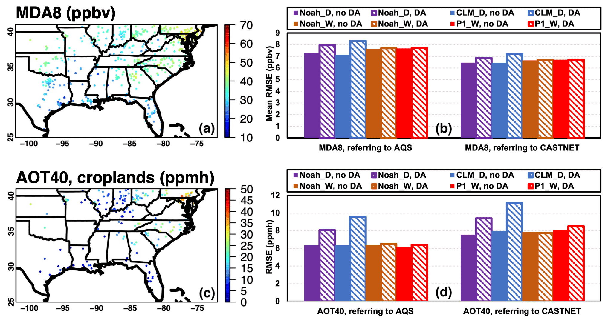
Figure 12 (a) Period-mean (16–28 August 2016) observed surface MDA8 O₃ and (c) AOT40 in cropland-dominant model grids derived from surface observations during 16–28 August 2016. The RMSEs of modeled MDA8 and model-derived AOT40 from various WRF-Chem cases referring to (a) and (c) are summarized in (b) and (d), respectively.

All model cases reproduced the observed MDA8 spatial patterns (Fig. 12a) moderately well. Referring to observations at AQS and CASTNET sites, their domain-wide mean root-mean-square errors (RMSEs) all fall within 6–8.5 ppbv (Fig. 12b). We first intercompare the MDA8 levels from all no-DA cases. Positive and negative differences between the results from Noah_W and P1_W, both of which implemented the Wesely scheme, are almost equally distributed across the domain, with the MDA8 from the former case associated with negligibly lower RMSEs (i.e., <0.02 ppbv on average) referring to AQS and CASTNET observations (Figs. 11k and 12b). The differences between these two cases are largely due to the impact of the chosen LSM on the model's meteorological fields, particularly temperatures, which affected the simulations of various O₃-related processes including dry deposition. As Figs. 11i and j and 12b show, replacing Wesely with the dynamic dry-deposition scheme considerably lowered the calculated MDA8 levels in majority of the model grids, as well as their associated RMSEs (i.e., by >0.5 ppbv on average) relative to surface observations. These reductions in MDA8 are of comparable magnitude with those due to updating anthropogenic emissions from the National Emission Inventory 2014 to 2016 beta (Huang et al., 2021). Comparing the implementations of the CLM- and Noah-type β schemes, the former led to stronger reductions in the modeled MDA8 fields and their associated uncertainty. These results reflect the impacts of the faster O₃ removal via dry deposition in the dynamic-scheme-related cases, as well as the different model meteorology. Our findings are qualitatively consistent with the conclusions from several global-scale modeling experiments that compared the Wesely and dynamic schemes (e.g., Val Martin et al., 2014; Lin et al., 2019).

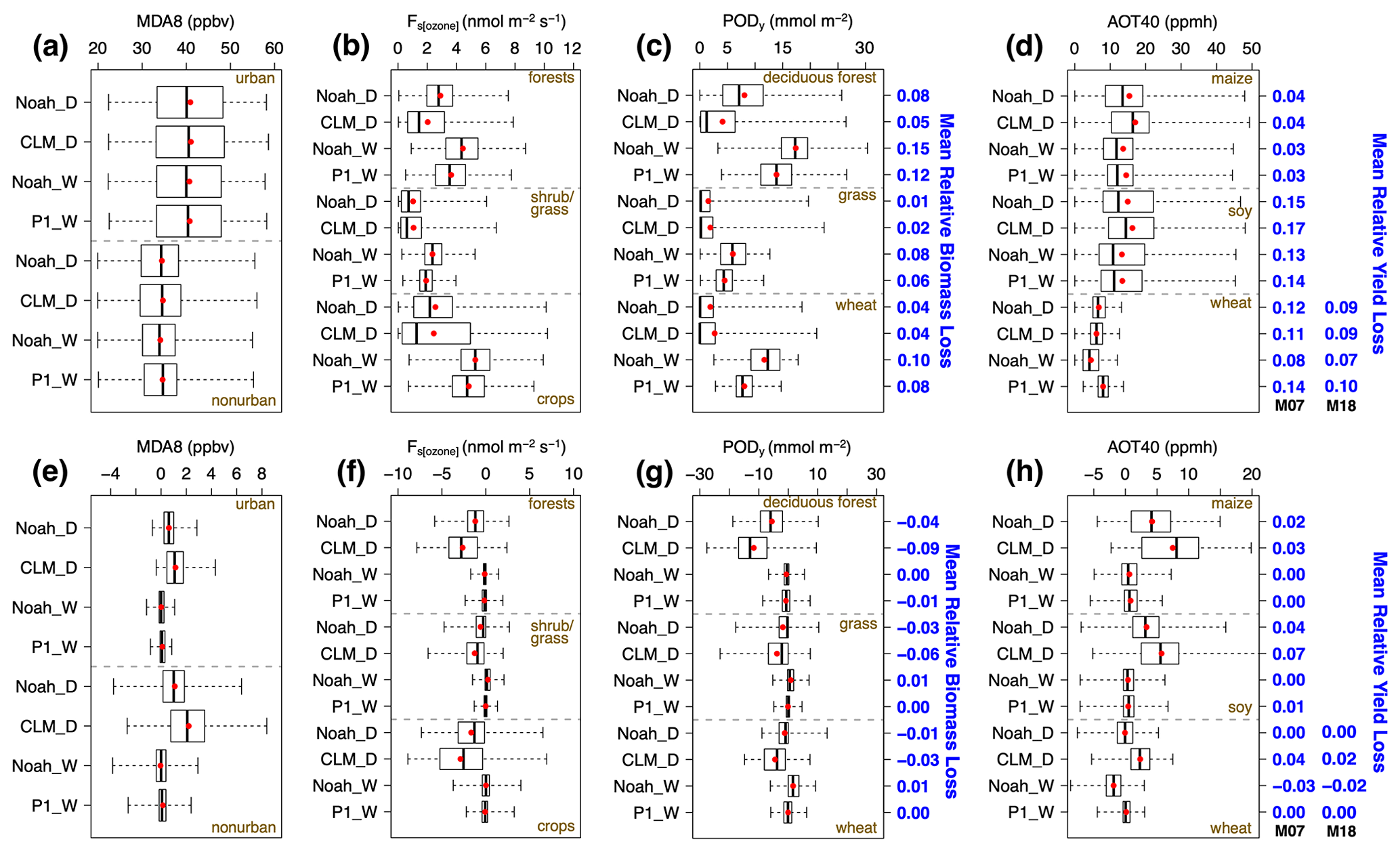
Figure 13 Box-and-whisker plots of WRF-Chem (a) MDA8 O₃, (b) daytime stomatal O₃ uptake F_s[ozone], (c) derived POD_y, and (d) derived AOT40, summarized by LULC and crop types from all DA-enabled cases. The impacts of the SMAP DA on these model fields are shown in (e)–(h). Red filled circles indicate the mean values. The mean relative biomass/crop yield losses estimated based on all DA-enabled cases, as well as the SMAP DA impacts on these values, are included in (c), (d), (g), and (h) in blue text. The crop yield losses for wheat, estimated based on the derived AOT40 and two dose–response functions (M07: Mills et al., 2007; M18: Mills et al., 2018b), are included in (d) and (h).

In all model cases, the DA reduced surface and subsurface SM in many of the grids, leading to enhanced MDA8 (Fig. 11e–h). The responses of the period-mean MDA8 to the DA from the Noah_W and P1_W cases are mostly within ±4 ppbv. When the dynamic dry-deposition scheme was applied, the modeled MDA8 responded several times more strongly to the DA (i.e., by up to 6 and 8 ppbv in the Noah_D and CLM_D cases, respectively), especially over nonurban regions, where surface MDA8 is on average several parts per billion by volume (ppbv) lower than in urban grids. In urban grids where population densities are ∼25 times higher than in nonurban grids (Fig. 1c), the DA impacts on MDA8 reach 3–4 ppbv in places, under the controls of the local-to-regional circulation patterns (Fig. 13a and e). As the no-DA cases are positively biased against surface observations in many places, corresponding to the DA-induced surface O₃ changes, the overall model performance of MDA8 was not improved, or much degraded, by the DA. Over limited areas such as the South Central Plains, the modeled MDA8 decreased due to the DA by up to >2 ppbv, corresponding to improved performance. The no-DA and DA results based on different LSMs and dry-deposition schemes confirm that drier soil conditions exacerbate O₃ air pollution, which, together with heat stress, threatens human health. Such O₃–SM relationships have also been demonstrated by Falk and Søvde Haslerud (2019) and Anav et al. (2018) using other chemical transport models and multiplicative dry-deposition schemes. Our Noah_W- and P1_W-related results indicate the influences of SM on air quality via its feedbacks to weather; and results from the Noah_D and CLM_D cases provide valuable information regarding both the indirect (i.e., via adjusting vegetation phenology and weather conditions) and direct SM effects on O₃. The complex SM impacts on O₃ dry-deposition as well as surface O₃ concentrations based on the coupled photosynthesis–r_s calculations rely heavily on the application of water stress function (β scheme), soil properties, and hydrological regime. The WRF-Chem results from this case indicate that, to more accurately simulate MDA8, improving land DA must be combined with strong efforts to identify other sources of uncertainty in O₃ modeling (e.g., emissions, chemistry, and extra-regional pollution contributions) and reduce their negative impacts on model performance.

Figure 14 Period-mean (16–28 August 2016) WRF-Chem (a–d) daytime stomatal O₃ uptake F_s[ozone] fields over terrestrial regions that do not belong to the urban category in Fig. 1a and (e–h) their responses to the SMAP DA. Results based on the (a, e) Noah_D, (b, f) CLM_D, (c, g) Noah_W, and (d, h) P1_W cases are shown.

3.3.2 Implications for O₃ vegetation impact assessments using concentration- and flux-based metrics

Both O₃ flux- and concentration-based metrics have been applied to assess O₃ impacts on vegetation as well as the associated economic loss. Estimating the plants' stomatal O₃ uptake F_s is the basis for constructing flux-based O₃ impact assessments. Figure 14 illustrates the period-mean daytime F_s fields based on all WRF-Chem no-DA cases as well as their responses to the SM DA. Box-and-whisker plots in Fig. 13b and f summarize these results by three LULC groups. The averaged F_s values for all three LULC groups exceed their respective critical levels (i.e., 1 nmol m⁻² s⁻¹ for forest and grasslands and 3 nmol m⁻² s⁻¹ for crops). As a major contributor to O₃ dry-deposition flux during the daytime, F_s fields appear to be closely correlated in space and time with the surface humidity and flux fields (e.g., GPP, latent heat, and EF, as well as v_d), which differ distinctly from the surface O₃ concentration fields. For example, F_s hotspots are shown over some low O₃ concentration areas including the humid, Lower Mississippi River regions, and the lowest F_s values occur in certain high O₃ concentration regions strongly affected by urban pollution (e.g., Georgia) and pollution transport from upwind US states and/or the stratosphere (e.g., western Kansas and Oklahoma, as discussed in Huang et al., 2021). The changes in F_s and surface O₃ concentrations due to the DA show opposite directions; i.e., drier soil enhances surface O₃ concentrations, whereas it slows down the plants' stomatal O₃ uptake (Figs. 11e–h and 14e–h). This comparison highlights how the choice of O₃ metrics can affect the assessment of O₃ vegetation impacts under the changing climate. As emphasized by Mills et al. (2018b) and Ronan et al. (2020), flux-based metrics have evident advantages over concentration-based metrics. To conduct reliable impact assessments using these flux-based metrics, accurate information on stomatal and non-stomatal fluxes as well as the various environmental and biophysical variables that they are sensitive to becomes increasingly important.

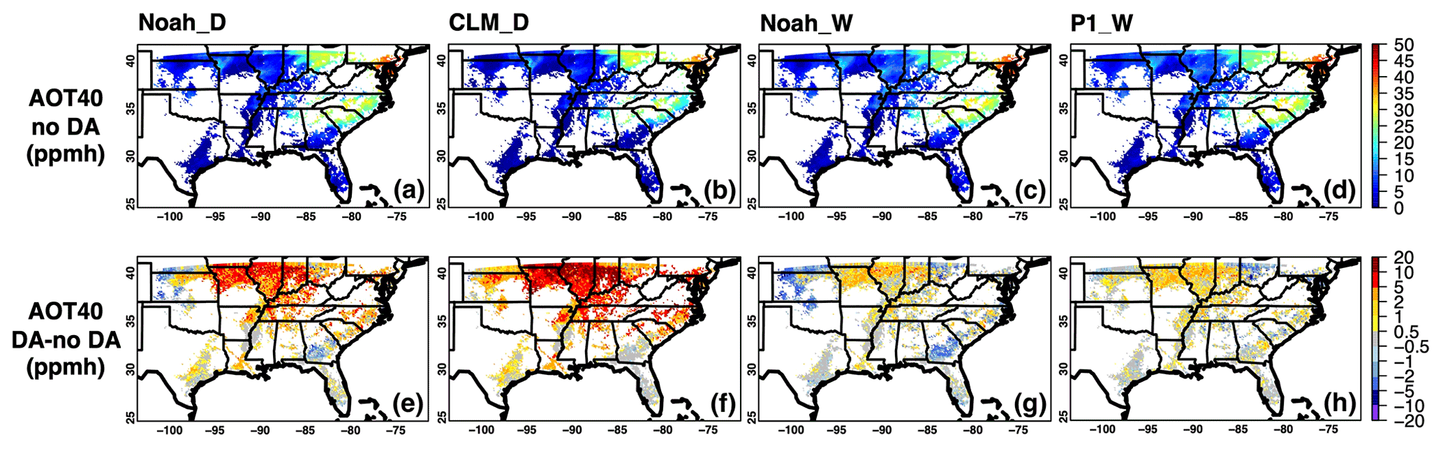
Figure 15 WRF-Chem-based AOT40, derived from the modeled surface O₃ fields during 16–28 August 2016, as well as their responses to the SMAP DA. Panels (a) and (e), (b) and (f), (c) and (g), and (d) and (h) show results derived from the Noah_D, CLM_D, Noah_W, and P1_W cases, respectively, in cropland-dominant model grids.

An assessment of O₃ vegetation impacts was conducted based on the results from various model cases and different metrics, namely POD_y (where y is the LULC-dependent critical level) and AOT40. For this demonstration, the 13 d model results were linearly extrapolated to approximately 3 months. This also assumed similar DA adjustments to SM dynamics (driven by factors such as clouds/radiation, rainfall, and irrigation for cropland-dominant regions) at the seasonal timescale. Based on the seasonal variability of surface O₃ and surface fluxes in the study region in 2016 (Fig. S6), the linearly scaled POD_y and AOT40 values are underestimated overall referring to the 2016 peak AOT40 and surface fluxes occurring during April–May–June and June–July–August, respectively. These overall underestimations may be invalid if the (sub)seasonal variability of surface O₃ and surface fluxes of other years was referred to. We therefore focus on discussing the results qualitatively and highlighting their implications for O₃ impact assessments using long-term records. Statistics of the derived POD_y and AOT40 fields are summarized by O₃-sensitive LULC and crop types in Fig. 13c, d, g, and h. Figures 15 and 12c and d present the estimated AOT40 fields and the evaluation of them, as well as their responses to the SM DA for cropland-dominant grids. The highs and lows in AOT40-related results are found over maize- and wheat-dominant fields, respectively. Among the three focused LULC types, the highest and lowest POD_y values are estimated for forests and grasslands, respectively. Largely driven by daytime peak O₃ concentrations, the spatial variability and biases (referring to AQS and CASTNET observations) of the model-derived AOT40 fields, as well as their responses to the DA, match those of the MDA8-based results (Fig. 11). In contrast, the spatial variability of POD_y and F_s aligns well, and so do their responses to the DA. Both POD_y and AOT40 reacted several times more intensively in the cases that implemented the dynamic dry-deposition scheme, especially the CLM_D case.

For selected LULC and crop types, the WRF-Chem-derived POD_y and AOT40 fields were used together with dose–response functions in literature to evaluate the RBL/RYL due to O₃ exposure and uptake. As reported in Fig. 13c and g, with the SM DA enabled, the mean RBLs based on Noah_D- and CLM_D-derived POD_y are 0.05–0.08, 0.01–0.02, and 0.04 for deciduous forest, grasslands, and wheat, respectively, which are >33 % lower than the Noah_W- and P1_W-based RBL estimates. It is shown that, in response to the DA which lowered SM in many places, the Noah_W- and P1_W-based RBL estimates did not drop as strongly as the Noah_D- and CLM_D-based ones and even increased by 0.01 for grasslands and wheat. For wheat, one of the most O₃-sensitive crops, the estimated RYL values based on the POD_y and AOT40 approaches differ by up to a factor of 2–3, and the DA had contrasting effects on these estimates (Fig. 13c, d, g, h). The POD_y- and AOT40-based RYL values differ more significantly when the model-derived POD_y and AOT40 fields came from the Noah_D and CLM_D cases. Using the model-derived AOT40 and different AOT40 dose–response functions (Mills et al., 2007, 2018b, Table 3), the estimated RYLs and their changes due to the DA are nonnegligible (Fig. 13d and h). Our estimated RBL/RYL results for various LULC and crop types mostly fall within the ranges reported in previous studies which applied model-derived O₃ metrics and dose–response functions (e.g., Avnery et al., 2011; Mills et al., 2007, 2018b). Our results emphasize that the selected O₃ impact assessment metrics for various LULC/crop types and their matching dose–response functions, as well as the model results used to derive the chosen O₃ metrics which are sensitive to dry-deposition schemes and SM, all introduce uncertainty to the estimated O₃ impacts on vegetation. The widely used dose–response functions are considered appropriate for studying North America and Europe, but they may not be applicable to other regions (Emberson et al., 2009). Therefore, updating and developing dose–response relationships for a larger number of vegetation types in different regions of the world are needed, which may require new experiments to be conducted. Yue and Unger (2014) and Lombardozzi et al. (2015), as well as follow-on investigations, parameterized the O₃ impacts on several types of vegetation using the relationships between cumulative O₃ uptake and O₃ damage factors for photosynthesis and conductance from empirical and experimental studies. Based on multidecadal model simulations, they reported <20 % changes of biomass, GPP, and energy fluxes due to O₃, which are roughly consistent with our RBL/RYL results in Fig. 13. Such approaches that dynamically assess the impacts of O₃ along with other factors (e.g., non-O₃ pollutants and environmental stresses), as highlighted in Emberson et al. (2018), will be considered in future work.

We note that, revising the dry-deposition scheme and constraining the modeled SM fields with observations would not only better be combined with adding O₃ impacts on vegetation but also multi-stress impacts on biogenic emissions. Considering O₃-induced vegetation injuries would more evidently affect longer-term climate simulations via feedbacks to biomass, surface fluxes, weather, and weather-driven emissions. As for biogenic emissions, Fig. S7 shows SM anomalies during the study period determined by our Noah-MP modeling system as well as drought stress activity factor γ_d estimated from β of a multiyear, independent CLM (version 4.5) simulation by Jiang et al. (2018). Based on this analysis, we estimate that, depending on soil type, hydrological regime, and β configurations, omitting the direct impacts of water stress on biogenic emissions may have introduced larger uncertainty (i.e., >30 %) to biogenic emission and O₃ modeling over several states experiencing drier-than-normal conditions, particularly South Carolina, Georgia, and Alabama. Quantitatively understanding the interplay between these processes and O₃ pollution levels is recommended for more accurate air quality modeling and O₃ impact assessments.

4 Summary and suggestions on future directions

This paper described a follow-up study of Huang et al. (2021). It presented how the choice of O₃ dry-deposition scheme affected our evaluation of SMAP SM DA impacts on coupled WRF-Chem modeling over the southeastern US in August 2016. In new Noah-MP LSM-related simulations, two dry-deposition schemes were implemented, namely the WRF-Chem default Wesely scheme and a dynamic scheme, in the latter of which the calculation of v_d (particularly its stomatal and cuticular terms) was modified to be coupled with photosynthesis and vegetation phenology. We showed that dry-deposition parameterizations significantly affected the modeled O₃ dry-deposition process, as well as its response to the DA. Comparing the no-DA cases, it was found that, when the dynamic scheme was applied, overall, the modeled O₃ dry-deposition velocities and fluxes were larger and surface O₃ concentrations were lower. The modeled O₃ fluxes responded 2–3 times more strongly to the SM changes due to the DA, which can be mainly explained by the fact that both the direct and indirect (i.e., via influencing weather and vegetation fields) effects of SM on O₃ dry-deposition modeling are considered in the dynamic scheme. Depending on soil type and hydrological regime, the selection of SM factor controlling r_s (i.e., β factor, a key variable representing the direct effects of SM on the modeled surface fluxes) scheme can strongly affect the quantitative results. The Wesely-scheme-derived dry-deposition results driven by meteorological fields from Noah-MP-based and (from Huang et al., 2021) Noah-LSM-based WRF-Chem simulations displayed much smaller differences than those due to updating the dry-deposition parameterizations. While we note that accounting for physiological effects in dry-deposition modeling can be beneficial, the Ball–Berry r_s scheme applied in land surface and dry-deposition modeling in this work needs to be compared with other semi-empirical r_s schemes, for a better understanding of their respective strengths and weaknesses. Alternative schemes include the Medlyn scheme, which has been integrated into the CLM version 5. Model intercomparison efforts such as the ongoing Air Quality Model Evaluation International Initiative Phase 4 activity (Galmarini et al., 2021) can also help determine areas for improvement in commonly used dry-deposition modeling approaches for studying 2016 and other years, over North America and other regions of the world.

By analyzing the model responses to the SM DA from these various cases, we conclude that, in coupled modeling systems that consider the direct and indirect influences of SM on O₃ dry deposition, the accuracy of SM is particularly critical to dry deposition and O₃ modeling, as well as the scientific analyses and impact assessments based on model simulations. The usefulness of SM DA for improving the modeled state and flux variables was evaluated by multiple observation(-derived) data products. Referring to in situ measurements, key meteorological variables relevant to v_d calculations such as surface temperature and humidity are shown to be improved by the DA by up to ∼9 %. Referring to satellite(-derived) datasets which may be associated with high uncertainty, the model performance of vegetation phenology, GPP, as well as energy fluxes and their partitioning, showed mixed, LULC-dependent reactions to the DA. According to the evaluation statistics, for this case, the CLM-type β factor scheme was slightly superior to the Noah-type one. The modeled carbon and energy fields, as well as their DA-related changes, correlated strongly with the modeled v_d fields, implying that the DA impacts on the accuracy of v_d were also possibly complicated, which is difficult to verify due to the lack of high-accuracy, independent v_d evaluation datasets, a point that has also been brought up in previous dry-deposition modeling works (e.g., Baublitz et al., 2020; Clifton et al., 2020). Observation(-derived) v_d datasets covering diverse LULC types nested in broad geographical regions and through more recent periods are in strong need. In places, the likely ineffectiveness of SM DA on vegetation and surface fluxes can not only be attributed to the quality of satellite SM retrievals and the DA approach used as discussed in previous Noah-LSM-based DA experiments, but also shortcomings in the Noah-MP LSM and its dynamic vegetation scheme regarding its surface–subsurface coupling and representation of SM-vegetation growth feedbacks. Continued efforts on advancing land measurement/retrieval skills and identifying and addressing deficits in LSMs, as well as practicing multivariate land DA, are recommended in future work.

This study also demonstrated that model-driven assessments of O₃ impacts on human health and various types of vegetation can be significantly affected by the applied O₃ dry-deposition scheme, the implementation of land DA, the chosen O₃ metrics, and their matching exposure–response functions. Various model cases showed that the DA impacts on MDA8 were more evident in nonurban areas where the mean MDA8 was ∼5 ppbv lower and the average population density is $<\mathrm{1}/\mathrm{25}$ of that in urban areas. Using concentration- and flux-based metrics AOT40 and POD_y, the mean RYLs of maize, soybean, and wheat fell within ranges of 0.01–0.04, 0.10–0.17, and 0.04–0.14, respectively. The multiple no-DA and DA cases helped us better understand the indirect and/or direct effects of SM on O₃ dry-deposition process, which have important implications for O₃ impact assessments. It is also recognized that the DA often exacerbated the positive surface O₃ biases in free-running systems, which has been a common issue shared by numerous regional and global models for this study region/season. It is necessary to combine land DA with efforts to identify, quantify, and reduce other sources of uncertainty in O₃ modeling. These should include reasonably representing the impacts of O₃ along with other factors on vegetation, the direct impacts of water stress on biogenic emissions of volatile organic compounds and nitrogen species, and the reduction of photolysis reaction rates and the modification of vertical transport due to the presence of foliage (Li et al., 2016; Jiang et al., 2018; Makar et al., 2017).