the Creative Commons Attribution 4.0 License.
the Creative Commons Attribution 4.0 License.
 | 21 Jul 2021
Satellite soil moisture data assimilation impacts on modeling weather variables and ozone in the southeastern US – Part 1: An overview
James H. Crawford
Joshua P. DiGangi
Gregory R. Carmichael
Kevin W. Bowman
Sujay V. Kumar
Xiwu Zhan
This study evaluates the impact of satellite soil moisture (SM) data assimilation (DA) on regional weather and ozone (O3) modeling over the southeastern US during the summer. Satellite SM data are assimilated into the Noah land surface model using an ensemble Kalman filter approach within National Aeronautics and Space Administration's Land Information System framework, which is semicoupled with the Weather Research and Forecasting model with online Chemistry (WRF-Chem; standard version 3.9.1.1). The DA impacts on the model performance of SM, weather states, and energy fluxes show strong spatiotemporal variability. Dense vegetation and water use from human activities unaccounted for in the modeling system are among the factors impacting the effectiveness of the DA. The daytime surface O3 responses to the DA can largely be explained by the temperature-driven changes in biogenic emissions of volatile organic compounds and soil nitric oxide, chemical reaction rates, and dry deposition velocities. On a near-biweekly timescale, the DA modified the mean daytime and daily maximum 8 h average surface O3 by up to 2–3 ppbv, with the maximum impacts occurring in areas where daytime surface air temperature most strongly (i.e., by ∼2 K) responded to the DA. The DA impacted WRF-Chem upper tropospheric O3 (e.g., for its daytime-mean, by up to 1–1.5 ppbv) partially via altering the transport of O3 and its precursors from other places as well as in situ chemical production of O3 from lightning and other emissions. Case studies during airborne field campaigns suggest that the DA improved the model treatment of convective transport and/or lightning production. In the cases that the DA improved the modeled SM, weather fields, and some O3-related processes, its influences on the model's O3 performance at various altitudes are not always as desirable. This is in part due to the uncertainty in the model's key chemical inputs, such as anthropogenic emissions, and the model representation of stratosphere–troposphere exchanges. This can also be attributable to shortcomings in model parameterizations (e.g., chemical mechanism, natural emission, photolysis and deposition schemes), including those related to representing water availability impacts. This study also shows that the WRF-Chem upper tropospheric O3 response to the DA has comparable magnitudes with its response to the estimated US anthropogenic emission changes within 2 years. As reductions in anthropogenic emissions in North America would benefit the mitigation of O3 pollution in its downwind regions, this analysis highlights the important role of SM in quantifying air pollutants' source–receptor relationships between the US and its downwind areas. It also emphasizes that using up-to-date anthropogenic emissions is necessary for accurately assessing the DA impacts on the model performance of O3 and other pollutants over a broad region. This work will be followed by a Noah-Multiparameterization (with dynamic vegetation)-based study over the southeastern US, in which selected processes including photosynthesis and O3 dry deposition will be the foci.
- Article
(18509 KB) - Full-text XML
- Companion paper
-
Supplement
(13504 KB) - BibTeX
- EndNote


Tropospheric ozone (O3) is a central component of tropospheric oxidation chemistry, with atmospheric lifetimes ranging from hours within polluted boundary layer to weeks in the free troposphere (Stevenson et al., 2006; Cooper et al., 2014; Monks et al., 2015). Ground-level O3 is a US Environmental Protection Agency (EPA) criteria air pollutant which harms human health and imposes threat to vegetation and sensitive ecosystems, and such impacts can be strongly linked or/and combined with other stresses, such as heat, aridity, soil nutrients, diseases, and non-O3 air pollutants (e.g., Harlan and Ruddell, 2011; Avnery et al., 2011; World Health Organization, 2013; Fishman et al., 2014; Lapina et al., 2014; Cohen et al., 2017; Fleming et al., 2018; Mills et al., 2018a, b). Across the world, various metrics have been used to assess surface O3 impacts (Lefohn et al., 2018). In October 2015, the US primary (to protect human health) and secondary (to protect public welfare including vegetation and sensitive ecosystems) National Ambient Air Quality Standards for ground-level O3, in the format of the daily maximum 8 h-average (MDA8), were revised to 70 parts per billion by volume (ppbv; US Federal Register, 2015). Understanding the connections between weather patterns and surface O3, as well as their combined impacts on human and ecosystem health under the changing climate, is important for the development of anthropogenic emission controls that are strong enough to meet target O3 air quality standards (Jacob and Winner, 2009; Doherty et al., 2013; Coates et al., 2016; Lin et al., 2017).
Ozone aloft is more conducive to rapid long-range transport to influence surface air quality in downwind regions (e.g., Zhang et al., 2008; Fiore et al., 2009; Hemispheric Transport of Air Pollution, HTAP, 2010, and references therein; Huang et al., 2010, 2013, 2017a; Doherty, 2015). In the upper troposphere–lower stratosphere regions, O3 as well as water vapor is particularly important to climate (Solomon et al., 2010; Shindell et al., 2012; Stevenson et al., 2013; Bowman et al., 2013; Intergovernmental Panel on Climate Change, 2013; Rap et al., 2015; Harris et al., 2015). Ozone variability in the free troposphere can be strongly affected by stratospheric air and transport of O3 that is produced at other places of the troposphere, as well as in situ chemical production from O3 precursors including nitrogen oxides (NOx, namely nitric oxide, NO, and nitrogen oxide, NO2), carbon monoxide (CO), methane, and non-methane volatile organic compounds (VOCs). Midlatitude cyclones are major mechanisms of venting boundary layer constituents, including O3 and its precursors, to the middle and upper troposphere. They are active throughout the year and relatively weaker during the summer. Convection, often associated with thunderstorms and lightning, is a dominant mechanism of exporting pollution in the summertime (e.g., Dickerson et al., 1987; Hess, 2005; Brown-Steiner and Hess, 2011; Barth et al., 2012). During North American summers, upper tropospheric anticyclones trap convective outflows and promote in situ O3 production from lightning and other emissions (e.g., Li et al., 2005; Cooper et al., 2006, 2007, 2009). It has also been shown that stratospheric O3 intrusions are often associated with cold frontal passages and convection (e.g., Pan et al., 2014; Ott et al., 2016).
On a wide range of spatial and temporal scales, atmospheric weather and composition interact with land surface conditions (e.g., soil and vegetation states, topography, and land use and land cover, LULC), which can be altered by various human activities and/or natural disturbances such as urbanization, deforestation, irrigation, and natural disasters (e.g., Betts et al., 1996; Kelly and Mapes, 2010; Taylor et al., 2012; Collow et al., 2014; Guillod et al., 2015; Tuttle and Salvucci, 2016; Cioni and Hohenegger, 2017; Fast et al., 2019; Schneider et al., 2019). As a key land variable, soil moisture (SM) influences the atmosphere via evapotranspiration, including evaporation from bare soil and plant transpiration. The SM–atmosphere coupling strengths are overall strong over transitional climate zones (i.e., the regions between humid and arid climates) where evapotranspiration is moderately high and constrained by SM (e.g., Koster et al., 2004, 2006; Seneviratne et al., 2010; Dirmeyer, 2011; Miralles et al., 2012; Gevaert et al., 2018). The southeastern US includes large areas of transitional climate zones, whose geographical boundaries vary temporally (e.g., Guo and Dirmeyer, 2013; Dirmeyer et al., 2013). Soil moisture and other land variables are currently measurable from space. It has been shown in a number of scientific and operational applications that satellite SM data assimilation (DA) impacts model skill of atmospheric weather states and energy fluxes (e.g., Mahfouf, 2010; de Rosnay et al., 2013; Santanello et al., 2016; Yin and Zhan, 2018). An effort began recently to evaluate the impacts of satellite SM DA on short-term regional-scale air quality modeling. Based on case studies in East Asia, such effects are shown to vary in space and time, partially dependent on surface properties (e.g., vegetation density and terrain) and synoptic weather patterns. Also, the SM DA impacts on model performance can be complicated by other sources of model error, such as the uncertainty of the models' chemical inputs including emissions and chemical initial and lateral boundary conditions (Huang et al., 2018).
This study extends the work by Huang et al. (2018) to the southeastern US during intensive field campaign periods in the summer convective season. Modified from the approach used in Huang et al. (2018), we assimilate satellite SM into the Noah land surface model (LSM) within National Aeronautics and Space Administration (NASA)'s Land Information System (LIS), which is semicoupled with the Weather Research and Forecasting model with online Chemistry (WRF-Chem). The term “semicoupled” indicates that the SM DA within LIS influences WRF-Chem's land initial conditions. Atmospheric states and energy fluxes from the no-DA and DA cases are compared with surface, aircraft, and satellite observations during selected field campaign periods. The WRF-Chem results are also compared with the chemical fields of the Copernicus Atmosphere Monitoring Service (CAMS), which serves as the chemical initial/lateral boundary condition model of WRF-Chem. Other sources of errors in WRF-Chem simulated O3 are identified by a WRF-Chem emission sensitivity simulation and the stratospheric O3 tracer output from the Geophysical Fluid Dynamics Laboratory (GFDL)'s Atmospheric Model, version 4 (AM4). The modeling and SM DA approaches as well as evaluation datasets are first introduced in Sect. 2. Section 3 starts with an overview of the synoptic and drought conditions during the study periods (Sect. 3.1), followed by discussions on the model responses to satellite SM DA. The SM DA impacts on O3 export from the US and the potential impacts on surface O3 in regions downwind of the US are included in the discussions. Results during a summer 2016 field campaign and a summer 2013 campaign are covered in Sect. 3.2–3.3 and 3.4, respectively. Section 4 summarizes key results from its previous sections, discusses their implications, and provides suggestions on future work.
2.1 Modeling and SM DA approaches
This study focuses on a summer southeastern US deployment (16–28 August 2016) of the Atmospheric Carbon and Transport (ACT)-America campaign (https://act-america.larc.nasa.gov, last access: 14 March 2021). One goal of this campaign is to study atmospheric transport of trace gases. Three WRF-Chem full-chemistry simulations (i.e., “base”, “assim”, and “NEI14” in Table 1) were conducted throughout this campaign on a 63 vertical layer, 12 km × 12 km (209×139 grids) horizontal-resolution Lambert conformal grid centered at 33.5∘ N, 87.5∘ W (Fig. 1a–c). To help confirm surface SM impacts on atmospheric conditions, a complementary simulation “minus001” was also conducted in the same model grid, only for selected events during this campaign (Table 1). Trace gases and aerosols were simulated simultaneously and interactively with the meteorological fields using the standard version 3.9.1.1 of WRF-Chem (Grell et al., 2005).
Table 1Summary of WRF-Chem simulations conducted in this study.
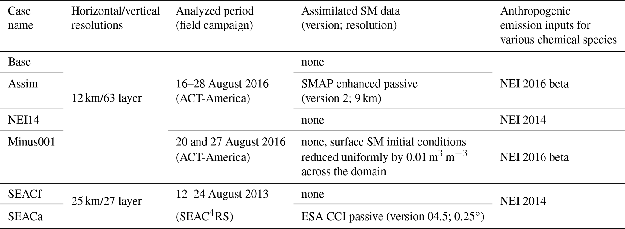
Acronyms are given as follows. ACT: Atmospheric Carbon and Transport; ESA CCI: European Space Agency Climate Change Initiative; NEI: National Emission Inventory; SEAC4RS: Studies of Emissions and Atmospheric Composition, Clouds and Climate Coupling by Regional Surveys; SM: soil moisture; SMAP: Soil Moisture Active Passive; WRF-Chem: Weather Research and Forecasting model with online Chemistry.
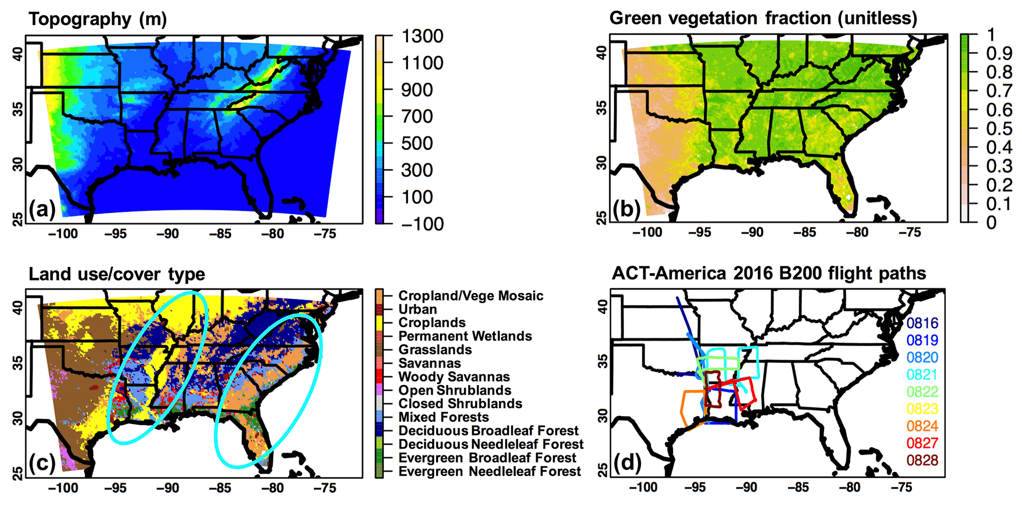
Figure 1(a) Terrain heights, (b) August 2016 green vegetation fraction, and (c) grid-dominant land use–cover categories used in the 12 km LIS/WRF-Chem simulations. (d) B-200 flight paths in the southeastern US during the 2016 ACT-America campaign. Cyan-blue circles in (c) denote the approximate locations of areas with high irrigation water use based on literature. Similar model domains and consistent sources of geographical inputs and meteorological forcings were used in 12 and 25 km LIS/WRF-Chem simulations.
Version 3.6 of the widely used, four-soil-layer Noah LSM (Chen and Dudhia, 2001) within LIS (Kumar et al., 2006) version 7.1rp8 served as the land component of the modeling/DA system used. An offline Noah simulation was performed within LIS prior to all WRF-Chem simulations for equilibrated land conditions (details in Sect. S1 in the Supplement). Consistent model grids and geographical inputs of the Noah LSM were used in the offline LIS and all WRF-Chem simulations. Specifically, topography, time-varying green vegetation fraction, LULC type, and soil texture type inputs were based on the Shuttle Radar Topography Mission Global Coverage-30 version 2.0, Copernicus Global Land Service, the International Geosphere-Biosphere Programme-modified Moderate Resolution Imaging Spectroradiometer (Fig. 1a–c), and the State Soil Geographic (Fig. S1, upper, in the Supplement; Miller and White, 1998) datasets, respectively.
Successful, valid retrievals of morning-time SM (version 2 of the 9 km enhanced product, generated using baseline retrieval algorithm) from NASA's Soil Moisture Active Passive (SMAP; Entekhabi et al., 2010) L-band polarimetric radiometer were assimilated into Noah within LIS. SMAP provides global coverage of surface (i.e., the top 5 cm of the soil column) SM within 2–3 d along its morning orbit (∼ 06:00 local time crossing) with the ground track repeating in 8 d. Compared to its predecessors that take measurements at higher frequencies, SMAP has a higher penetration depth for SM retrievals and lower attenuation in the presence of vegetation. Evaluation of SMAP data over North America with in situ and LSM output suggests better data quality over flat and less forested regions (Pan et al., 2016), and previous studies have demonstrated that the SMAP DA improvements on weather variables are more distinguishable over regions with sparse vegetation (e.g., Huang et al., 2018; Yin and Zhan, 2018). Before the DA, SMAP data were re-projected to the model grid and bias correction was applied via matching the means and standard deviations of the Noah LSM and SMAP data for each grid (de Rosnay et al., 2013; Huang et al., 2018; Yin and Zhan, 2018) during August 2015–2019. Such bias correction reduced the dynamic ranges of SM from the original SMAP retrievals. The Global Modeling and Assimilation Office (GMAO) ensemble Kalman filter approach embedded in LIS was applied, with the ensemble size of 20. Perturbation attributes of state variables (Noah SM) and meteorological forcing variables (radiation and precipitation) were based on default settings of LIS derived from Kumar at al. (2009).
All WRF-Chem cases, except the minus001 case, were started on 13 August 2016. Atmospheric meteorological initial and lateral boundary conditions were downscaled from the 3-hourly, 32 km North American Regional Reanalysis (NARR). Consistent with NARR, the WRF-Chem model top was set at 100 hPa, slightly above the climatological tropopause heights for the study region and month. The National Centers for Environmental Prediction (NCEP) daily sea surface temperature (SST) reanalysis product was used as an additional WRF forcing. Chemical initial and lateral boundary conditions for major chemical species were downscaled from the 6-hourly, -level CAMS. Surface O3 from CAMS is positively biased over the eastern US referring to various observations, but major chemical species in the free troposphere are overall successfully reproduced (e.g., Huijnen et al., 2020; Wang et al., 2020). As WRF-Chem only has tropospheric chemistry, the lack of dynamic chemical upper boundary conditions is expected to introduce biases in the modeled O3 throughout the troposphere, and such biases depend on the distribution of model vertical layers, as well as the length of the simulation. To determine how this limitation of WRF-Chem affects its O3 performance, we used the outputs (3-hourly, -level) from GFDL's AM4 (Horowitz et al., 2020) and its stratospheric O3 tracer, which have been applied to other O3 studies (e.g., Zhang et al., 2020). Since the second day of the simulation period, chemical initial conditions were cycled from the chemical fields of the previous day's simulation. Atmospheric meteorological and land fields were reinitialized every day at 00:00 UTC with NARR and the previous day's no-DA or DA LIS outputs, respectively. Each day's simulation was recorded hourly at 00:00 (minute:second) through the following 30 h, forced by temporally constant SST as the diurnal variation of the sea surface is typically smaller than land on large scales. Each day's WRF-Chem meteorological outputs served as the forcings of the no-DA and DA LIS simulations, which produced land initial conditions for the next day's WRF-Chem simulations. The model output >6 h since each day's initialization was analyzed for the period of 16–28 August 2016.
In all WRF-Chem simulations, key physics options applied include the local Mellor–Yamada–Nakanishi–Niino planetary boundary layer (PBL) scheme along with its matching surface layer scheme (Nakanishi and Niino, 2009), the Rapid Radiative Transfer Model short- and longwave radiation schemes (Iacono et al., 2008), the Morrison double-moment microphysics, which predicts the mass and number concentrations of hydrometeor species (Morrison et al., 2009), and the Grell–Freitas scale-aware cumulus scheme (Grell and Freitas, 2014), which has also been implemented in the GMAO GEOS-Forward Processing system (https://gmao.gsfc.nasa.gov/news/geos_system_news/2020/GEOS_FP_upgrade_5_25_1.php, last access: 14 March 2021). Chemistry-related configurations are the Carbon-Bond Mechanism version Z (Zaveri and Peters, 1999) gas-phase chemical mechanism and the eight-bin sectional Model for Simulating Aerosol Interactions and Chemistry (MOSAIC; Zaveri et al., 2008), including aqueous chemistry for resolved clouds. Both aerosol direct and indirect effects were enabled in all simulations.
Daily biomass burning emissions came from the Quick Fire Emissions Dataset (Darmenov and da Silva, 2015) version 2.5r1, and plume rise with a recent bug fix (suggested by Ravan Ahmadov, NOAA/ESRL, in August 2019) was applied. Emissions of biogenic VOCs and soil NO were computed online (i.e., driven by the WRF meteorology) using the Model of Emissions of Gases and Aerosols from Nature (MEGAN; Guenther et al., 2006). It has been shown that MEGAN may overpredict biogenic VOC emissions over the study regions and tends to underpredict soil NO emissions, especially in high-temperature (i.e., >30 ∘C) agricultural regions (e.g., Oikawa et al., 2015; Huang et al., 2017b, and references therein). Important sources of uncertainty include the following: (1) there is uncertainty in MEGAN's land and meteorological inputs, including surface temperature and radiation fields from WRF; and (2) drought influences on these emissions are not well understood and represented in MEGAN, and such influences include biogenic VOC emissions being enhanced, reduced, or terminated during various stages of droughts. Specifically, at the early stage of droughts when plants still have sufficient reserved carbon resources, dry conditions may promote these emissions via enhancing leaf temperature. Persistent droughts will terminate biogenic VOC emissions after the reserved carbon resources are consumed (e.g., Pegoraro et al., 2004; Bonn et al., 2019). Cloud-top-height-based lightning parameterization was applied (Wong et al., 2013). The intra-cloud to cloud-to-ground flash ratio was based on climatology (Boccippio et al., 2001), and lightning NO was distributed using vertical profiles in Ott et al. (2010). For both intra-cloud and cloud-to-ground flashes, 125 mol of NO was emitted per flash, close to the estimates in several studies for the US (e.g., Pollack et al., 2016; Bucsela et al., 2019). The passive lightning NOx tracer was implemented, which experienced atmospheric transport but not chemical reactions. Anthropogenic emissions in the base, assim, and minus001 simulations (Table 1) were based on US EPA's National Emission inventory (NEI) 2016 beta, and NEI 2014 was used in the NEI14 simulation. The differences between NEI 2016 beta and earlier versions of NEIs, such as NEI 2014 and 2011, are summarized at http://views.cira.colostate.edu/wiki/wiki/10197/inventory-collaborative-2016beta-emissions-modeling-platform (last access: 27 March 2020), for various chemical species. Anthropogenic emissions of O3 precursors are lower in NEI 2016 beta than in NEI 2014 (by <20 % for key species) as well as NEI 2011, in which NOx emissions may be positively biased for 2013 (Travis et al., 2016). These differences are qualitatively consistent with the observed trends of surface air pollutants (https://www.epa.gov/air-trends, last access: 27 March 2020).
Chemical loss via dry deposition (i.e., dry deposition velocity vd multiplied by surface concentration) was calculated based on the widely used Wesely scheme (Wesely, 1989; details in Sect. S2). This scheme defines vd as the reciprocal of the sum of aerodynamic resistance, quasi-laminar sublayer resistance, and surface resistance. Over the land, surface resistance, the major component of vd, is classified into stomatal–mesophyll and several other resistance terms. Surface resistance is usually strongly affected by its stomatal–mesophyll resistance term which in the Wesely scheme is expressed as season- and LULC-dependent constants, which are subject to large uncertainty, being adjusted by surface temperature and radiation. This contrasts with some other approaches which also account for the influences of SM, vapor pressure deficit (VPD), and vegetation density in adjusting these constants and which couple stomatal resistance with photosynthesis. For calculating the other surface resistance terms, prescribed season- and LULC-dependent constants are used in the Wesely scheme, adjusted by environmental variables including surface wetness, radiation, and temperature, whereas in other existing schemes, impacts of friction velocity and vegetation density are also considered (e.g., Charusombat et al., 2010; Park et al., 2014; Val Martin et al., 2014; Wu et al., 2018; Mills et al., 2018b; Anav et al., 2018; Wong et al., 2019; Clifton et al., 2020, and references therein). Aerodynamic resistance and quasi-laminar resistance are both sensitive to surface properties such as surface roughness.
This paper also briefly discusses in Sect. 3.4 some results from two WRF-Chem simulations (i.e., “SEACf” and “SEACa” in Table 1) during the 2013 Studies of Emissions and Atmospheric Composition, Clouds and Climate Coupling by Regional Surveys (SEAC4RS; Toon et al., 2016; https://espo.nasa.gov/home/seac4rs/content/SEAC4RS, last access: 14 March 2021) campaign. SEAC4RS studies the attribution and quantification of pollutants and their distributions as a result of deep convection. These simulations were conducted on a 27 vertical layer, 25 km × 25 km (99×67 grids) horizontal-resolution Lambert conformal grid, also centered at 33.5∘ N, 87.5∘ W. Their LSM and inputs, WRF physics and chemistry configurations were the same as those used in the 12 km cases described above. In SEACa, we assimilated successfully retrieved, daily SM from version 04.5 of the European Space Agency Climate Change Initiative project (ESA CCI) SM product (Gruber et al., 2019), developed on a horizontal-resolution grid based on measurements from passive satellite sensors. The assimilated CCI SM data were re-projected to the model grid and bias-corrected based on the climatology of Noah and CCI SM during August 1999–2018. These simulations were evaluated with SEAC4RS aircraft chemical observations, which were richer than those collected during ACT-America in terms of the diversity of measured reactive chemical compounds (Sect. 2.2.1). Such comparisons help evaluate the emissions of O3 precursors from various (e.g., NEI 2014 anthropogenic, lightning, and biogenic) sources as well as how the model representation of land–atmosphere interactions affects such emission assessments.
The model horizontal resolutions of 12 and 25 km were set to be close to the assimilated satellite SM products to minimize the horizontal representation errors. At these resolutions, land surface heterogeneity and fine-scale processes (e.g., cloud formation and turbulent mixing) may not be realistically represented. Cloud-top-height-based lightning emissions and SM–precipitation feedbacks can be highly dependent on convective parameterizations (e.g., Hohenegger et al., 2009; Wong et al., 2013; Taylor et al., 2013). Addressing shortcomings of convective parameterizations in simulations at these scales is still in strong need. Performing convection-permitting simulations with assimilation of downscaled microwave SM or/and high-resolution thermal-infrared-based SM (e.g., 2–8 km from the Geostationary Operational Environmental Satellite) for cloudless conditions should also be experimented on in the future.
2.2 Evaluation datasets
2.2.1 Aircraft in situ measurements during ACT-America and SEAC4RS
During the 2016 ACT-America deployment, the NASA B-200 aircraft took meteorological and trace gas measurements in the southeastern US from the surface to ∼300 hPa on 9 d. Different line colors in Fig. 1d denote individual flight paths during this period. These flights were conducted under different weather conditions during the daytime (i.e., within 14:00–23:00 UTC, local time +6), with durations of 4–9 h (https://www-air.larc.nasa.gov/missions/ACT-America/reports.2019/index.html, last access: 14 March 2021). Flights on 16, 20, and 21 August 2016 sampled the air under stormy weather conditions, whereas the other flights were conducted under fair weather conditions. We used meteorological as well as collocated O3 and CO measurements collected on the B-200 to evaluate our WRF-Chem simulations. The O3 mixing ratio measurements using the differential ultraviolet absorption has a 5 ppbv uncertainty (Bertschi and Jaffe, 2005), and the CO mixing ratio was measured with an uncertainty of 10 ppbv, using a Picarro analyzer which is based on wavelength-scanned cavity ring down spectroscopy (Karion et al., 2013). We used the weather and trace gas observations averaged in 1 min intervals (version R1, released in November 2020) for model evaluation, as they represent atmospheric conditions on comparable spatial scales to the model. Ozone and CO measurements with mol mol−1 (Travis et al., 2016) are assumed to be influenced by fresh stratospheric intrusions and were excluded in our analysis. This approach, however, was rather arbitrary and may not have excluded air that had an aged stratospheric origin or mixtures of air with different origins.
Aircraft (NASA DC-8) in situ measurements of CO, NO2, and formaldehyde (HCHO) from the surface to ∼200 hPa during six SEAC4RS daytime (i.e., within 13:00–23:00 UTC, local time +6), 8–10 h science flights in August 2013 were compared with our WRF-Chem simulations. The CO mixing ratio was measured using the tunable diode laser spectroscopy technique, with an uncertainty of 5 % or 5 ppbv. The NO2 measurements were made by two teams, based on thermal dissociation laser-induced fluorescence and chemiluminescence methods, with an uncertainty of ±5 % and (0.030 ppbv +7 %), respectively. Two other teams took the HCHO measurements, using a compact atmospheric multispecies spectrometer and the laser-induced fluorescence technique, with the uncertainty of ±4 % and (0.010 ppbv ±10 %), respectively. Aircraft data averaged in 1 min intervals (version R7, released in November 2018) were used, with the biomass-burning-affected samples (acetonitrile >0.2 ppbv) and CO from fresh-stratospheric-intrusion-affected air ( mol mol−1) excluded.
2.2.2 Ground-based measurements
WRF-Chem results were evaluated by various surface meteorological and chemical observations. These include the following: (1) SM values observed at ∼5 and ∼10 cm below the surface, which were measured at various sites within the Soil Climate Analysis Network (SCAN), were downloaded from the International Soil Moisture Network (Dorigo et al., 2011) and screened by quality flags before being used. (2) Surface air temperature (T2), relative humidity (RH; derived from the original dew point and air temperature data), and wind speed (WS) from the NCEP Global Surface Observational Weather Data were utilized. (3) Half-hourly or hourly latent and sensible heat fluxes measured using the eddy covariance method at eight sites within the FLUXNET network were used. Latent and sensible heat fluxes from this network exhibited mean errors of −5.2 % and −1.7 %, respectively (Schmidt et al., 2012). We only analyzed the modeled energy fluxes at the sites where the model-based LULC classifications are realistic. A , daily FLUXCOM product was also utilized, which merges FLUXNET data with machine learning approaches, remote sensing, and meteorological data. Over North America, it is estimated that latent and sensible heat fluxes from this FLUXCOM product are associated with ∼12 % and ∼13 % of uncertainty, respectively (Jung et al., 2019). (4) Hourly O3 observed at the US EPA Air Quality System (AQS; mostly in urban/suburban regions) and the Clean Air Status and Trends Network (CASTNET; mostly in nonurban areas) sites also played an important role in this study. Hourly AQS and CASTNET O3 are US sources of the Tropospheric Ozone Assessment Report database, the world's largest collection of surface O3 data supporting analysis on O3 distributions, temporal changes and impacts. Measurements of NO2 and HCHO are also available at some of the AQS sites. It is highly possible that these measurements are biased due to the interferences of other chemical species and therefore they were not used in this work.
2.2.3 Precipitation products
The WRF-Chem precipitation fields were also qualitatively compared with two precipitation data products: (1) the 4 km, hourly NCEP Stage IV Quantitative Precipitation Estimates product (Lin and Mitchell, 2005), which is a widely used, national radar- and rain-gauge-based analysis product mosaicked from 12 River Forecast Centers over the contiguous US, and of which quality partially depends on the manual quality control done at the River Forecast Centers; and (2) the , half-hourly calibrated rainfall estimates from version 6B of the Integrated Multi-satellitE Retrievals for the Global Precipitation Measurement (GPM) constellation final run product (Huffman et al., 2019a). Compared with single-platform-based precipitation products, multisensor-based precipitation datasets have reduced limitations and therefore have become popular in scientific applications. Nevertheless, these datasets may be associated with region-, season-, and rainfall-rate- dependent uncertainties (e.g., Tan et al., 2016; Nelson et al., 2016, and references therein).
3.1 Overview of the synoptic and drought conditions during the study periods
In August 2016, several states in the southern US experienced moderately to extremely moist conditions according to major drought indexes such as the Palmer Hydrological Drought Index (Fig. S2, left). These were largely due to the influences of passing cold fronts and tropical systems from the Gulf of Mexico (https://www.ncdc.noaa.gov/sotc/synoptic/201608, last access: 14 March 2021). Temperatures were consequently lower than normal in these regions. Contrastingly, controlled by the Bermuda High, more frequent air stagnation and warmer- and drier-than-normal conditions affected multiple Atlantic states. Opposite hydrological anomalies were recorded during August 2016 and August 2013 for the Southern Great Plain and Atlantic regions (Fig. S2, left).
The anomalies in synoptic patterns and drought conditions in August 2016 and 2013, as well as the day-to-day weather changes, can partially explain the regional O3 variability in the southeastern US. Based on the pressure gradients along the western edges of the Bermuda High (Zhu and Liang, 2013; Shen et al., 2015), the influences of the Bermuda High on southeastern US surface O3 enhancements may be stronger in August 2016 than in August 2013 (Fig. S2, middle). Lightning intensities and emissions respond to climate change (Romps et al., 2014; Murray, 2016; Finney et al., 2018), therefore affecting the probability of fires ignited by lightning. Based on satellite detections which are subject to cloud contamination, fire activities associated with emissions of heat and O3 related pollutants were stronger in drier regions in the southern US in August 2016 and 2013. The variable synoptic and drought conditions also controlled biogenic VOC and soil NO emissions as well as O3-related chemical reaction and deposition rates, and the resulting impacts on O3 depended on the changing anthropogenic NOx emissions (Hudman et al., 2010; Hogrefe et al., 2011; Coates et al., 2016; Lin et al., 2017). In the upper troposphere, troughs bumping into the anticyclone above the southeastern US in August 2016 helped shape the pollution outflows differently than in August 2013 when the North American monsoon anticyclone was built over the southwestern US, and the central-eastern US was controlled by a strong cool trough (Fig. S2, right).
Studies have shown that the variations in land–atmosphere coupling strength are connected with SM interannual variability and the local spatiotemporal evolution of hydrologic regime (e.g., Guo and Dirmeyer, 2013; Tuttle and Salvucci, 2016). Therefore, over the Southern Great Plain and Atlantic regions, SM–atmosphere coupling strengths in August 2016 and August 2013 may have diverged from the climatology in opposite directions. For example, in August 2016, the overall potential impacts of SM on surface water and energy fluxes and atmospheric states may be higher than normal over the Atlantic regions and below the average in the Southern Great Plain. In August 2013, the land–atmosphere coupling may be stronger than normal and abnormally weak over the Southern Great Plain and the Atlantic regions, respectively.
3.2 Soil moisture, weather states, and energy fluxes during ACT-America
Land and surface weather states as well as energy fluxes from the WRF-Chem base simulation, together with the SMAP DA impacts on these variables, are illustrated in Fig. 2 (for SM), Figs. 3–4 (for T2, RH, WS, and PBL height, PBLH), Fig. 5 (for precipitation), and Figs. 6, S3, and S4 (for energy fluxes and their partitioning) for the 16–28 August 2016 period.
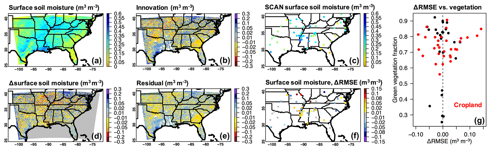
Figure 2Period-mean (16–28 August 2016) (a) WRF-Chem base case surface-layer (i.e., 0–10 cm belowground) soil moisture at initial times and (d) its changes due to the SMAP DA. Panels (b, e) indicate the SMAP DA impacts on the discrepancies between SMAP and modeled surface soil moisture. Panel (c) presents soil moisture measurements at various SCAN sites at ∼10 cm belowground at WRF-Chem initial times. The SMAP DA impacts on RMSEs of the modeled surface soil moisture, as well as their relationships with the model-based green vegetation fraction, are shown in (f, g). In (g), the SCAN sites located in cropland areas according to the model's land use–cover input are highlighted in red.
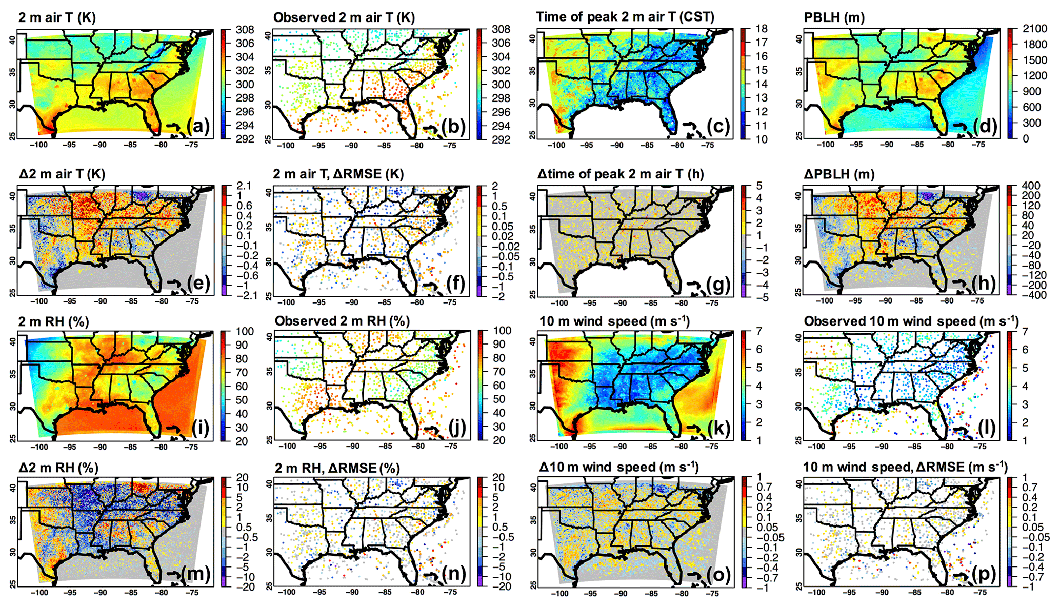
Figure 3Period-mean (16–28 August 2016) WRF-Chem base case daytime (a) 2 m air temperature (T); (d) PBLH; (i) 2 m relative humidity (RH); and (k) 10 m wind speed, as well as (e, h, m, o) the impacts of SMAP DA on these model fields. Observed daytime surface T, RH, and wind speed, as well as the impacts of the SMAP DA on RMSEs of these model fields are shown in (b, f), (j, n), and (l, p) respectively. Significance test results are included in Fig. 4. The time of daily peak air T in US central standard time (CST), as well as its response to the SMAP DA, is shown in (c, g).
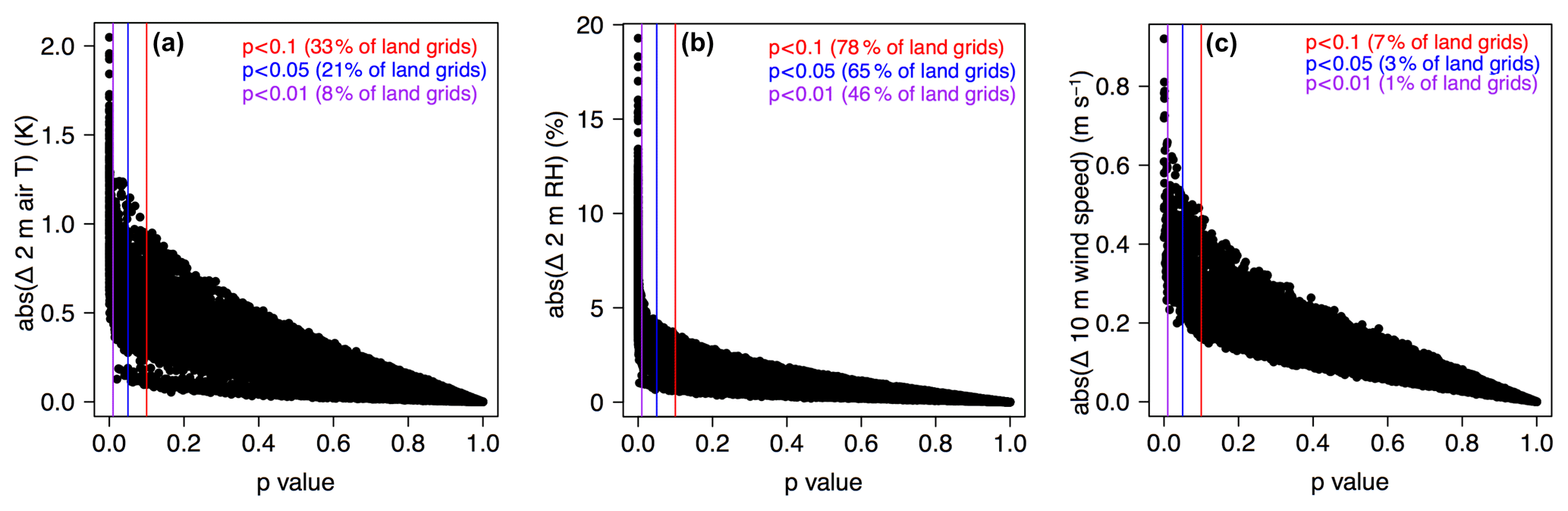
Figure 4The p values of Student's t tests comparing the daytime (a) 2 m air temperature (T); (b) 2 m relative humidity (RH); and (c) 10 m wind speed from the base and assim cases, plotted against the absolute changes in these model fields due to the SMAP DA. Results are only presented for the overland model grids.
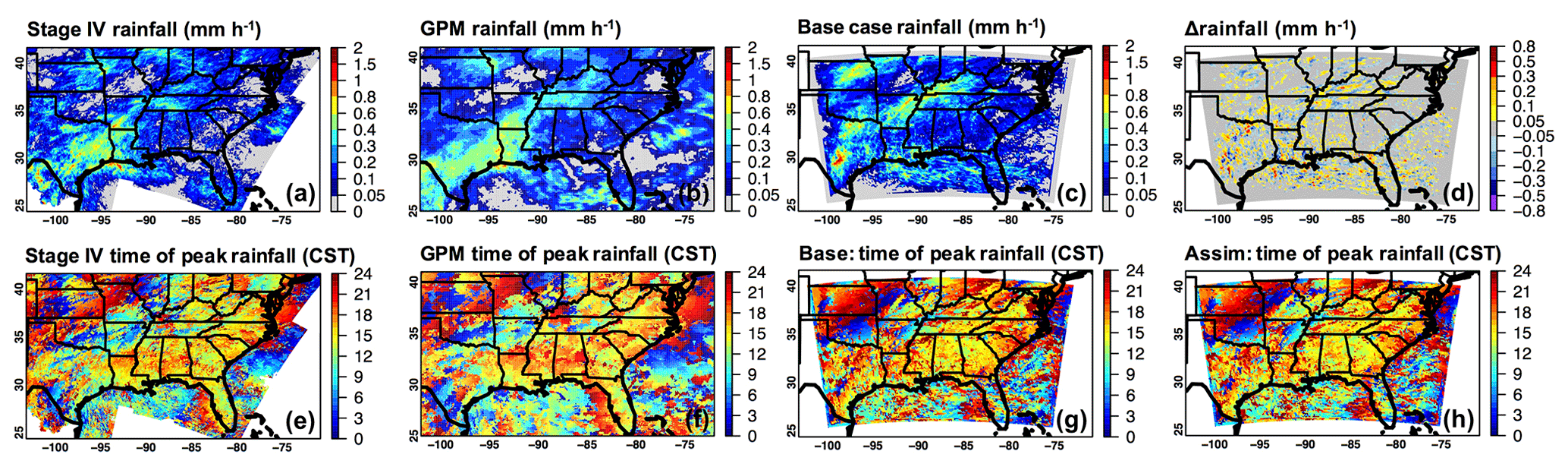
Figure 5Period-mean (16–28 August 2016) (a–d) rainfall rate and (e–h) time of peak rainfall in US central standard time (CST) from (a, e) the National Stage IV Quantitative Precipitation Estimates product; (b, f) the Global Precipitation Measurement; and (c, g) the WRF-Chem base case. The impacts of the SMAP DA on WRF-Chem results are indicated in (d, g, h).
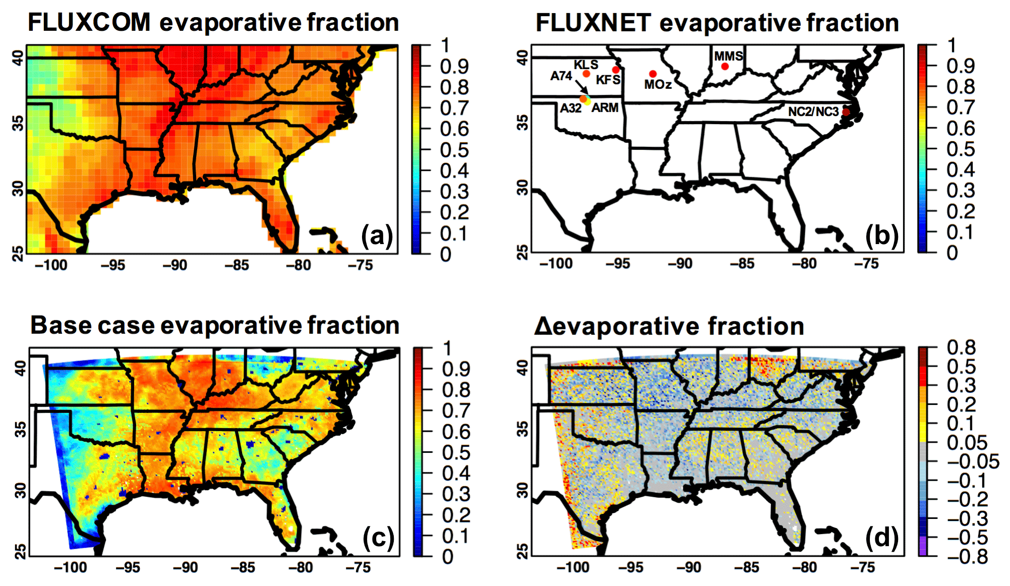
Figure 6Period-mean (16–28 August 2016) daily evaporative fraction, defined as daily latent heat (daily latent heat + daily sensible heat), from (a) a FLUXCOM product; (b) selected FLUXNET sites; and (c) the WRF-Chem base case. Panel (d) shows the impact of the SMAP DA on WRF-Chem evaporative fraction. Additional evaluation results for latent and sensible heat fluxes at the focused FLUXNET sites are presented in Fig. S3.
3.2.1 Observed and modeled SM and weather conditions
The highest daytime (13:00–24:00 UTC, local time +5 or +6) average T2 was observed in several states in the Atlantic region that were undergoing drought conditions (Figs. S2, left; 3b). The daily T2 maxima occurred during noon–early afternoon in most places, consistent with the findings from Huang et al. (2016). The Lower Mississippi River regions were influenced by high humidity (Fig. 3j). Under the influence of the Bermuda High, surface winds were overall mild to the east of Texas. Strongest rainfall affected Texas, Arkansas, Kentucky, Tennessee, and near the border of Kansas and Missouri (Fig. 5a–b), which belonged to the wetter-than-normal regions according to August 2016 drought indexes. Rainfall in most areas peaked in the late afternoon or evening after the times of peak T2 (Fig. 5e–f). The observed diurnal cycles of rainfall and T2 indicate that, for the study area/period, convection was mainly due to the thermodynamic response to surface temperature. However, land–sea interactions, fronts, and topography, as well as aerosol loadings may also have come into play.
The dry and wet anomalies in the southeastern US based on the modeled SM (Fig. 2a) are shown to be consistent with ground-based SM measurements (e.g., Fig. 2c), as well as weekly (not shown in figures) and monthly drought indexes (e.g., Fig. S2, left). The modeled SM values in various soil layers are near the model-based soil wilting points and field capacities (Fig. S1, middle and lower) over drought-influenced and wetter-than-normal regions, respectively. The WRF-Chem base simulation overall captured the observed patterns of T2, RH, and WS across the domain, with its daytime PBLH spatially correlated with the T2 patterns (Table 2 and Figs. 3a–b; d; i–j; k–l). Referring to the Stage IV and GPM rainfall data, the WRF-Chem base case also reproduced the diurnal cycles of rainfall during the study period fairly well overall, but the rainfall hotspots simulated by the model appear west to those in the Stage IV and GPM products (Fig. 5c). Dirmeyer et al. (2012) found that models' rainfall performance more strongly depended on the distinctive treatment of the model physics than on the model resolution. Our WRF-Chem performance for rainfall diurnal cycle in this region is similar to previous convection-permitting WRF-Chem simulations (e.g., Barth et al., 2012). Additionally, the WRF-Chem predicted mean rainfall rates over low-precipitation regions (e.g., several Atlantic states) are higher than those based on the Stage IV and GPM rainfall products, which tend to overestimate precipitation at the low end (e.g., Nelson et al., 2016; Tan et al., 2016). Such positive model biases for low-precipitation regions have also been reported in Barth et al. (2012).
Table 2The SMAP DA impacts on modeled surface meteorological and O3 fields, as well as their agreement with observations.
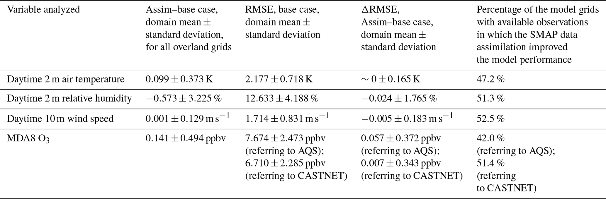
Acronyms: AQS: Air Quality System; CASTNET: Clean Air Status and Trends Network; MDA8: daily maximum 8 h average; RMSE: root-mean-square error; SMAP: Soil Moisture Active Passive.
3.2.2 SMAP DA impacts on SM, surface weather states and energy fluxes
Surface SM at the model initial times (i.e., 00:00 UTC each day) was broadly reduced by the SMAP DA, except parts of coastal Texas, Ohio, and Florida (Fig. 2d). Such changes in the modeled SM fields are consistent with the modeled daytime specific humidity (not shown in figures) and RH responses (Fig. 3m). They are anti-correlated with the model responses in the averaged daytime T2 and PBLH fields (Fig. 3e; h) as well as their daily amplitudes (not shown in figures). The daytime T2 and RH responses to the SMAP DA are statistically significant in ∼21 % and ∼65 % of the overland model grids, respectively (i.e., p<0.05 based on Student's t tests; Fig. 4a–b), with the most significant daytime-averaged responses of ∼2 K and >10 %, respectively, occurring in Missouri and Ohio, as well as several other states located within 33–40∘ N and 90–100∘ W. In places, the daily maxima of WRF-Chem T2 were delayed by an hour or two when the SMAP DA was enabled (Fig. 3g). The changes in WRF-Chem temperature gradients due to the SMAP DA led to slight WS enhancements over many of the model grids (Fig. 3o). In contrast to the WRF-Chem T2 and RH responses, these WS changes are statistically insignificant (i.e., p>0.05 based on Student's t tests) in ∼97 % of the overland model grids (Fig. 4c). On the 13 d timescale, the SMAP DA had less discernable impacts on rainfall, consistent with the findings from Koster et al. (2010, 2011) and Huang et al. (2018). The SMAP DA impacts on mean rainfall rate and diurnal cycles show noisy patterns (Fig. 5d; g; h), and positive and negative SM–precipitation relationships are both found. The spatial and temporal variability in these model sensitivities reflects the impacts of local hydrological regimes and their anomalies, as well as moisture advection.
It is indicated by Fig. 2b and e that, during the study period, the SMAP DA successfully reduced the discrepancies between SMAP and Noah-calculated surface SM across the model domain. The modeled surface SM was also cross-validated with ground-based SM measurements at dozens of SCAN sites, using the root-mean-square error (RMSE) metric. Figure 2f–g show the results based on a comparison of the modeled surface SM with ∼10 cm belowground SM measurements at these SCAN sites. This evaluation suggests that the Noah-based SM was more evidently improved by the SMAP DA at sparsely vegetated regions; i.e., RMSE was reduced at almost all sites where green vegetation fraction ≤0.6. At dense-vegetation (i.e., green vegetation fraction >0.6) SCAN sites, over a half of which are located in cropland areas subject to the impacts of irrigation and other human activities, the SMAP DA did not prevalently decrease or increase the discrepancies between the modeled and measured SM. Similar findings were reached based on such a comparison of the modeled surface SM and ∼5 cm belowground SM measurements at these SCAN sites. The overall T2, RH, and WS performance of WRF-Chem was not prevalently improved or degraded due to the inclusion of the SMAP DA (e.g., Fig. 3f; n; p, based on the RMSE metric); i.e., improvements on T2, RH, and WS occurred in 47 %, 51 %, and 52 % of the model grids where observations are available, and the domain-wide mean RMSE changes for T2, RH, and WS are ∼0 K, −0.024 %, and −0.005 m s−1, respectively (Table 2). This finding for dense vegetation regions is qualitatively consistent with the findings in Huang et al. (2018) and Yin and Zhan (2018), which are based on RMSE and other evaluation metrics, and it may partially be attributed to SMAP retrieval quality and the land–atmosphere feedbacks represented in Noah. Additionally, as discussed in Huang et al. (2018), unrealistic model representations of terrain height can pose challenges for evaluating the modeled surface weather fields with ground-based observations. The 12 km model grid used in this work represents terrain height well (i.e., |model–actual m) at over 70 % of the model grids that have collocated observations, but at some locations the discrepancies between the model and actual terrain height exceed 100 m. Furthermore, human activities such as irrigation can significantly modify water budget and land–atmosphere coupling strength over agricultural regions (e.g., Lu et al., 2017), but these processes were unaccounted for in the modeling system used. Observations from SMAP and other satellites are capable of detecting the signals of irrigation over the southeastern US (e.g., the circled regions in Fig. 1c based on Ozdogan and Gutman, 2008, and Zaussinger et al., 2019) and other regions of the world. However, for locations where irrigation or/and other missing processes dominantly contributed to the systematic biases between the modeled and SMAP SM, the bias correction approach applied may have removed the information of these processes from the SMAP observations before the DA. As a result, the DA may not be effective at these locations. How irrigation patterns and scheduling, depending in part on the weather conditions, affected our WRF-Chem performance, as well as the effectiveness of the SMAP bias correction and DA, is worth further investigations. In places, the changes in WRF-Chem rainfall patterns due to the SMAP DA are within the discrepancies between the Stage IV and GPM rainfall products. A better understanding of the uncertainty associated with these two rainfall products used can benefit the assessment of SM DA impacts on the model's precipitation performance.
The spatial patterns of evaporative fraction (defined as latent heat (latent heat + sensible heat)) follow those of SM and RH, with the maxima (>0.75) seen in the Lower Mississippi River region and smaller values (<0.65) in the dry Atlantic states and some parts of the Southern Great Plains (Fig. 6a–b). Note that the absolute latent and sensible heat fluxes can differ significantly at locations with similar evaporative fraction values (Fig. S3). The WRF-Chem-based evaporative fraction shows similar spatial gradients but is overall negatively biased (Fig. 6c). The changes in WRF-Chem evaporative fraction due to the SMAP DA are spatially correlated with the surface moisture changes (Figs. 2d; 3m; 6d). As a result, the model performance of evaporative fraction was only improved over some of the regions where it was increased by the SMAP DA. It is found that the SMAP DA impacts on model performance are not universally consistent for surface energy fluxes and land–atmosphere states. This can be explained by the fact that the modeling system used has shortcomings in representing SM–flux coupling and/or the relationships between moisture and heat fluxes and the atmospheric weather which need to be clearly identified and corrected. The most possible reasons causing such model behaviors include the following: (1) irrigation and other processes related to human activities were unaccounted for, and the surface exchange coefficient CH, which is a critical parameter controlling energy transport from the land surface to the atmosphere, may not be realistically represented in Noah (details in Sect. S1); (2) the SMAP DA did not update the vegetation and surface albedo fields in Noah, which was unrealistic; and (3) soil parameters determined from soil texture types and a lookup table may be inaccurate in places. To confirm and address these limitations in the modeling/DA system used, and to identify other possible reasons, future efforts should be devoted to applications using other LSMs (e.g., the Noah-Multiparameterization) and up-to-date inputs and parameters (e.g., soil texture types and lookup tables), together with multivariate land DA; evaluation of additional water and energy flux variables such as runoff and radiation, the latter of which shows inconsiderable sensitivities to the SMAP DA (Fig. S4); and utilization of alternative WRF inputs and physics configurations.
3.2.3 SMAP DA impacts on weather conditions at various altitudes
The WRF-Chem-modeled weather states were also evaluated with ACT-America aircraft observations at various altitudes. Along the flight paths, the observed air temperature and water vapor mixing ratios decrease with altitude, which were captured by WRF-Chem fairly well (Figs. 7a–b; e–f and 8a; c). The modeled air temperature and humidity as well as their responses to the SMAP DA vary in space and time. In general, these responses are particularly strong near the surface, where the majority of the samples were collected. Under stormy weather conditions on 16, 20, and 21 August 2016, the maximum changes in air temperature and humidity in the free troposphere exceed 2.3 K and 2 g kg−1, respectively (Fig. 7c; g). Corresponding to these changes, the SMAP DA modified the RMSEs of WRF-Chem air temperature and/or water vapor by over 5 % for several individual flights and reduced the RMSEs of these model variables overall by ∼0.7 % and ∼2.3 %, respectively (Fig. 8b). The most significant improvements in the modeled weather states occurred at ≥800 hPa, where the maximum improvements in air temperature and water vapor exceed 2.6 K and 2 g kg−1, respectively, and their RMSEs were both reduced by ∼2.7 % (Figs. 7d; h and 8d).
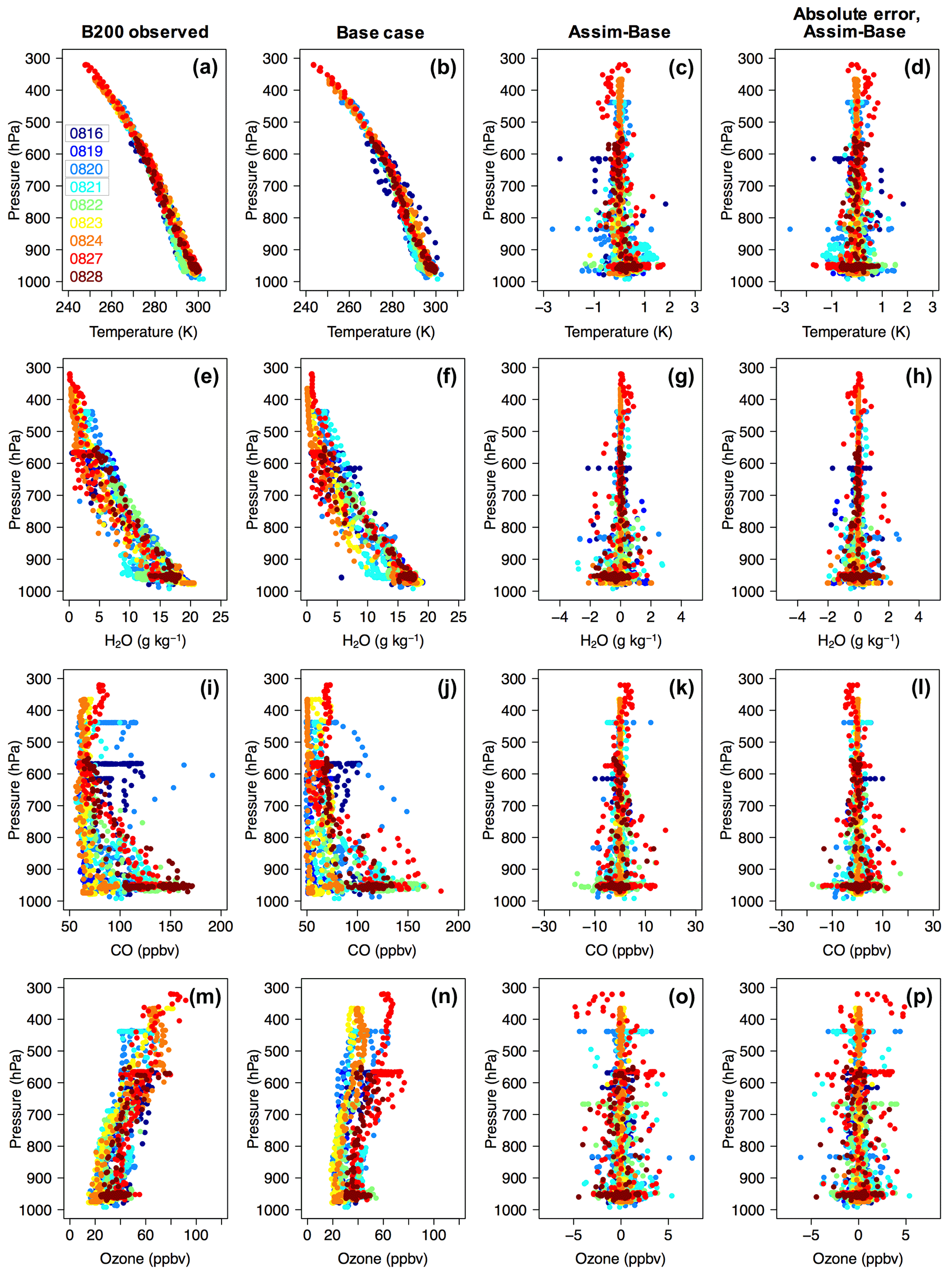
Figure 7Vertical profiles of (a) air temperature; (e) water vapor mixing ratio (H2O); (i) carbon monoxide (CO); and (m) O3 observed on the B-200 aircraft during the ACT-America 2016 campaign, based on a 1 min averaged dataset. Their WRF-Chem counterparts from the base case and the impacts of the SMAP DA are shown in (b, f, j, n) and (c, g, k, o), respectively. The SMAP DA impacts on model performance along these flights, based on the absolute error metric (i.e., |modeled–observed|), are indicated in (d, h, l, p). The different colors distinguish samples taken on various flight days, and the B-200 paths on these flight days are shown in Fig. 1d. Flights on 16, 20, and 21 August 2016 were conducted under stormy weather conditions as highlighted in (a), whereas the B-200 flew under fair weather conditions during other flights.
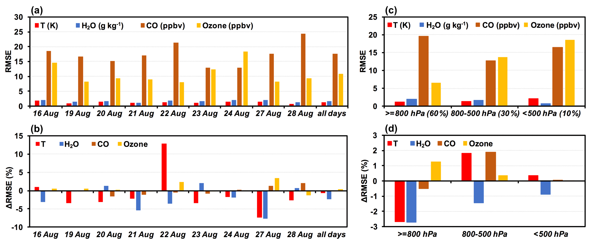
Figure 8Evaluation of WRF-Chem results with the B-200 aircraft observations during the ACT-America 2016 campaign: (a, c) the RMSEs of air temperature (T), water vapor mixing ratio (H2O), carbon monoxide (CO), and O3 of the model base case; and (b, d) the impacts of the SMAP DA on RMSEs of these variables. Panels (a, b) and (c, d) summarize the model performance by flight day and flight altitude range, respectively. The B-200 flight paths by day are shown in Fig. 1d. Proportions of ∼60 %, ∼30 %, and ∼10 % of the related aircraft observations were taken at ≥800, 800–500, and <500 hPa, respectively.
3.3 Ozone and its responses to the SMAP DA during ACT-America
3.3.1 Surface O3
The changes in the above-discussed meteorological variables (e.g., air temperature, humidity, WS, PBLH) due to the SMAP DA alter various atmospheric processes which can have mixed impacts on surface O3 concentrations. For example, warmer environments promote biogenic VOC and soil NO emissions as well as accelerating chemical reactions (e.g., many oxidation processes, thermal decomposition of peroxyacetyl nitrate). These will be discussed in detail in the following paragraphs referring to Figs. 9 and S5. Faster winds and thickened PBL dilute air pollutants including O3 and its precursors and therefore reduce O3 destruction via titration (i.e., ) as well as photochemical production of O3. The changes in wind vectors affect pollutants' concentrations in downwind regions. Water vapor mixing ratios perturb O3 photochemical production and loss via affecting the HOx cycle. Their impacts on O3 levels depend on the chemical environments of the areas of interest; i.e., in general, reduced specific humidity slightly enhances O3, except in some polluted regions. Also, higher RH is often associated with cloud abundance and solar radiation and therefore slows down the photochemical processes (Camalier et al., 2007). Additionally, chemical loss via stomatal uptake may be slower under lower SM and humidity and higher temperature conditions, and nonstomatal uptake also varies with meteorology. These processes, however, may not all be realistically represented by the Wesely dry deposition scheme (Sects. 2.1 and S2; Figs. S1 and S7) used in this study.
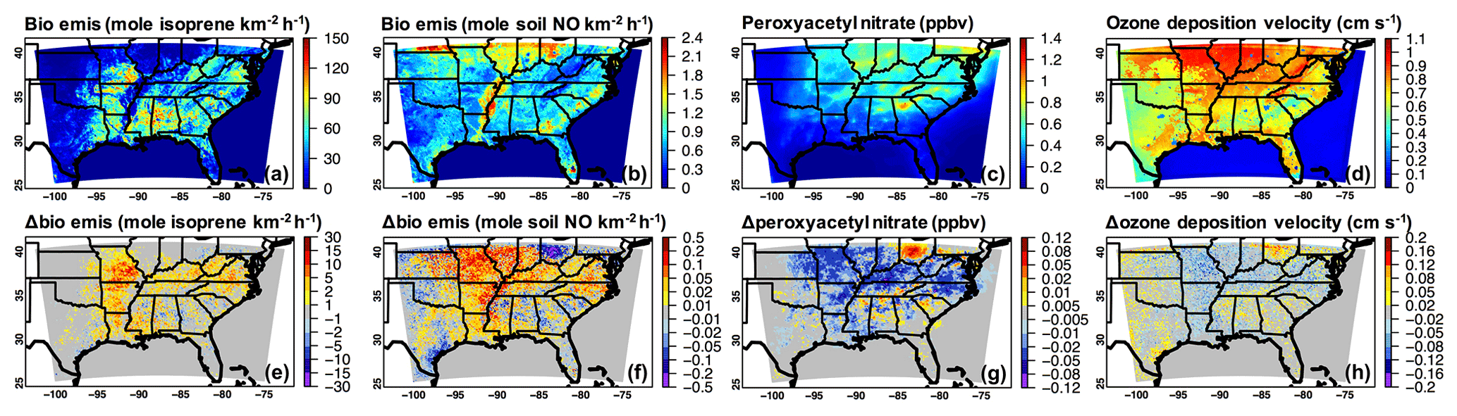
Figure 9Period-mean (16–28 August 2016) WRF-Chem base case daytime biogenic emissions of (a) isoprene and (b) soil nitric oxide (NO); (c) surface peroxyacetyl nitrate concentration; and (d) O3 deposition velocity, as well as (e–h) the impacts of SMAP DA on these model fields. Additional results of these variables are shown in Fig. S5.
Figure 10a–b compare the observed and WRF-Chem base case daytime surface O3 during 16–28 August 2016, and the SMAP DA impacts on daytime surface O3 are shown in Fig. 10c. Low-to-moderate O3 pollution levels are seen over most areas within the model domain, except the Atlantic states due to the influences of frequent air stagnation and warm and dry conditions. Period-mean daytime surface O3 responses to the SMAP DA are overall slightly positive but exceed or closely approach 2 ppbv in some places in Missouri, Illinois, and Indiana, and the strongest decreases in the period-mean daytime surface O3 occurred in Ohio (i.e., by >2 ppbv). The averaged O3 changes show strong spatial correlations (with correlation coefficient r values of ∼0.8) with those of T2 and PBLH (Fig. 3e; h), which are anti-correlated with the surface humidity responses (Figs. 2d and 3m). On most of the days during 16–28 August 2016, the maximum impacts of SMAP DA on daily daytime surface O3 exceed 4 ppbv, and the O3 sensitivities are moderately correlated with the daytime T2 changes (Fig. 11a, with r values within 0.4–0.7). The period-mean WRF-Chem surface MDA8 and its response to the SMAP DA (Fig. 12a–b) show similar spatial patterns to those of the modeled surface daytime O3 but are of higher variability.
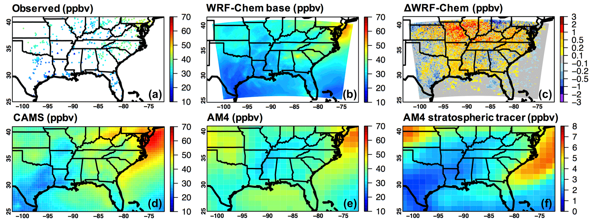
Figure 10Period-mean (16–28 August 2016) daytime surface O3 from (a) the EPA AQS (filled circles) and CASTNET (triangles) sites; (b) WRF-Chem base case; (d) CAMS; and (e) GFDL AM4. Panel (c) shows the impact of the SMAP DA on WRF-Chem-modeled daytime surface O3. Panel (f) indicates stratospheric influences on daytime surface O3 based on the AM4 stratospheric O3 tracer output.
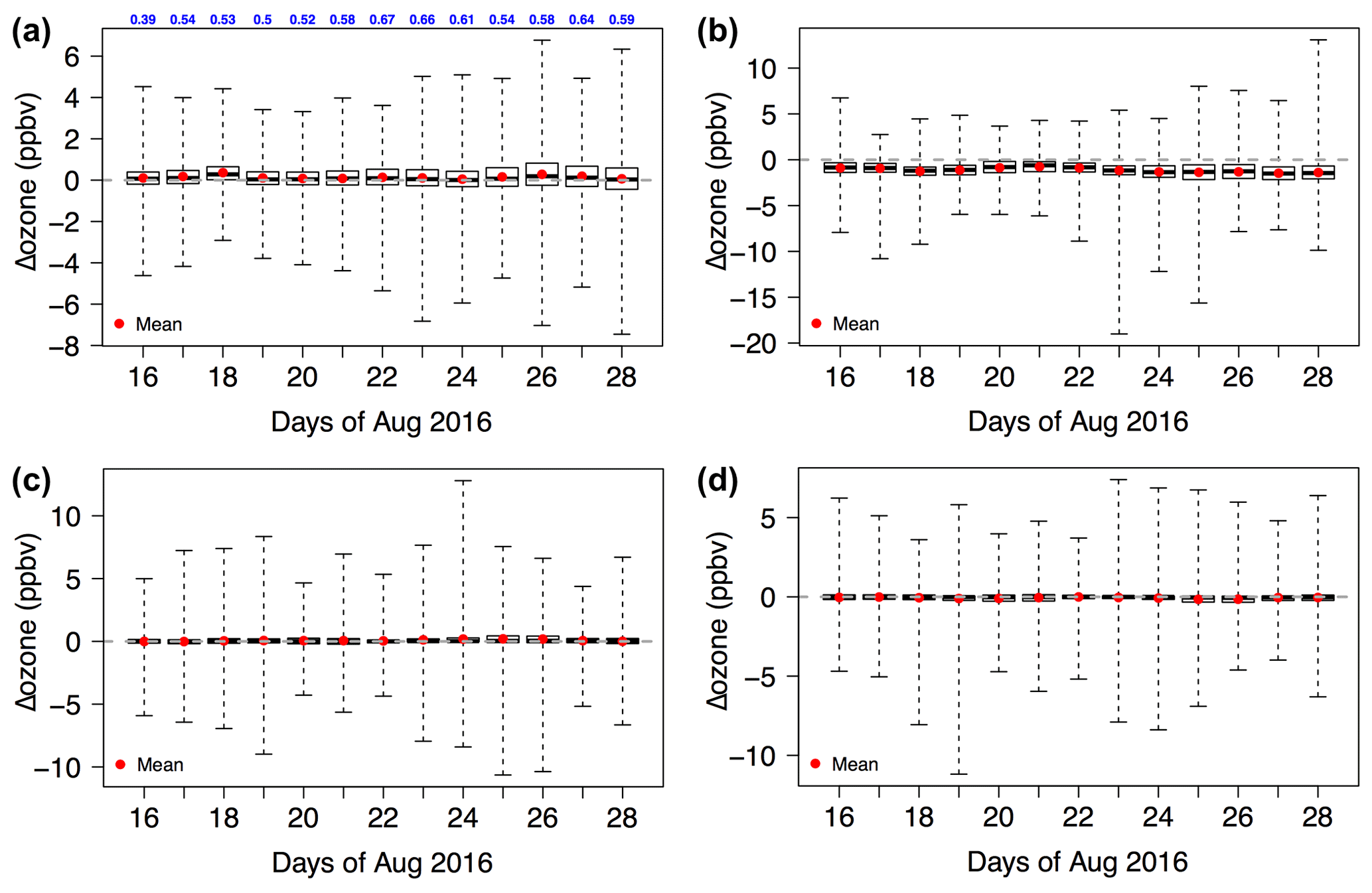
Figure 11Box-and-whisker plots of WRF-Chem daytime O3 responses to (a, c) the SMAP DA; and (b, d) updating anthropogenic emissions from NEI 2014 to NEI 2016 beta. Panels (a–b) and panels (c–d) show O3 changes at the surface (only for terrestrial model grids, 68 % of all model grids) and at ∼400 hPa (in all model grids), respectively. Blue text in (a) shows spatial correlation coefficients r between WRF-Chem daily daytime 2 m air temperature changes and O3 changes due to the SMAP DA. Note the different y-axis ranges.
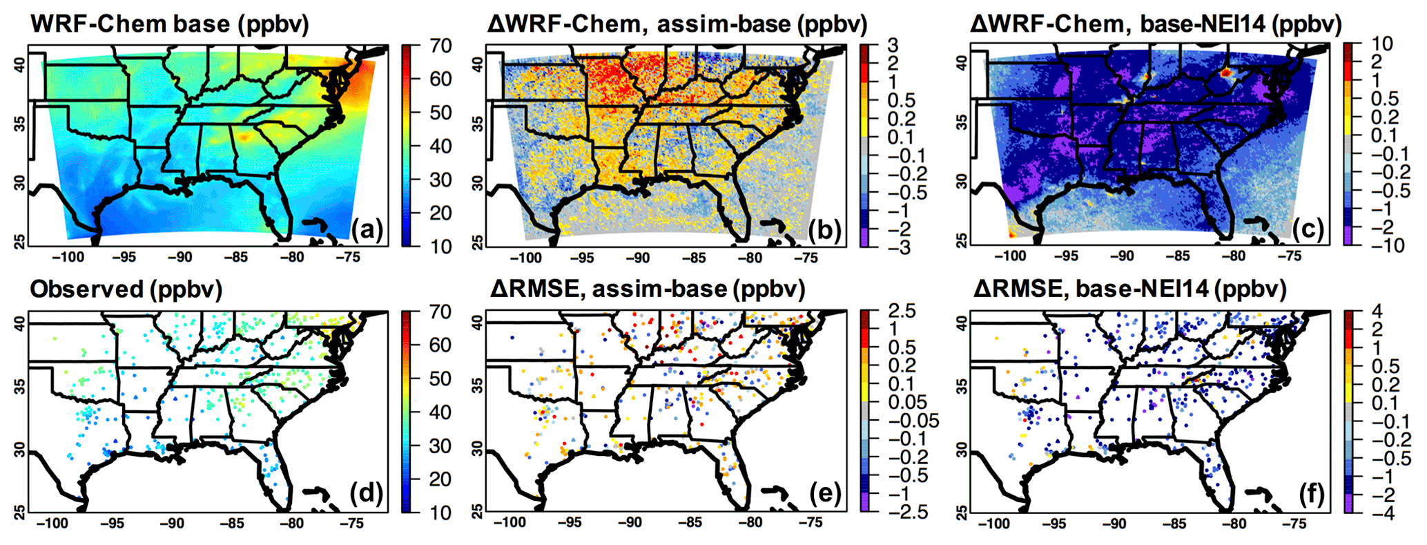
Figure 12Period-mean (16–28 August 2016) daily maximum 8 h average (MDA8) surface O3 from (a) the WRF-Chem base case and (d) the EPA AQS (filled circles) and CASTNET (triangles) sites. The impact of the SMAP DA on WRF-Chem MDA8 O3 and the associated RMSE changes are shown in (b, e). The benefit of using NEI 2016 beta instead of NEI 2014 is indicated in (c, f).
The overall enhanced biogenic emissions of VOCs and soil NO (Figs. 9a–b; e–f and S5, first two rows) belong to the major causes of the changes in the surface daytime-average and MDA8 O3 described above. The SMAP DA impacts on MEGAN biogenic emissions were largely due to its impact on T2 (Fig. 3e). This is because the modeled photosynthetically active radiation (PAR), which is another variable critical to estimating biogenic emissions of some species, shows only ≪10 % of responses to the SMAP DA in most places (Fig. S4, lower), and based on previous analyses of MEGAN emission-PAR sensitivities (e.g., Fig. 2 in Guenther et al., 2012), it is estimated that these changes in modeled PAR have caused negligible impacts on the modeled biogenic emissions. MEGAN biogenic emissions were most strongly modified over the regions with elevated emissions, i.e., by >20 % over the Missouri Ozarks for isoprene and by >10 % over agricultural land for soil NO, where emission factors at standard conditions are high, and the DA-induced T2 changes are strong and statistically significant. Over the Missouri Ozarks, the >20 % isoprene emission changes corresponding to the ∼2 K T2 changes are consistent with the previously reported isoprene emission sensitivities to surface air temperature (e.g., Huang et al., 2017b, and references therein). MEGAN's limitations in representing biogenic VOC emission responses to drought may have had minor impacts on most of the high-biogenic-emission regions which were not affected by drought during this period. For certain parts of the Atlantic states that were in the early–middle phases of drought in August 2016 (referring to drought indexes from July to October 2016 which are not shown in figures), while it is highly likely that the reserved carbon resources were still available, and leaf temperature still controlled the VOC emissions, the lack of SM dependency in MEGAN VOC emission calculations may have introduced uncertainty to the results from both the base and the assim cases. However, as the SMAP DA only mildly affected SM and T2 over these regions (Figs. 2d and 3e), we do not anticipate that biogenic VOC emissions would be changed significantly there by the SMAP DA, even if their dependencies on SM were realistically included in MEGAN. Also, note that for this case, satellite-based leaf area index data were used in MEGAN biogenic VOC emission calculations. Although satellite-based leaf area index data may be more accurate than those calculated by dynamic vegetation models, they are less temporally variable than the reality, and the SMAP DA did not adjust this critical MEGAN input. These also limited the responses of MEGAN-calculated VOC emissions (and thus O3-related chemical fields) to the DA. Uncertainty in the modeled soil NO emissions and their responses to the SMAP DA may be larger over high-temperature cropland regions. This needs further investigations accounting for the influences of SM, which is controlled by both precipitation and human activities such as irrigation, as well as the fertilization conditions.
The overall accelerated chemical reactions, including those strongly controlling the lifetime of peroxyacetyl nitrate, are also highly responsible for the above-mentioned changes in surface daytime-average and MDA8 O3. For example, in broad regions north of 33∘ N, the modeled daytime-mean surface peroxyacetyl nitrate concentrations show 10 %–20 % responses to the SMAP DA, and these responses are mostly in the opposite directions of the T2 and surface O3 changes (Fig. 9c; g). This reflects that the increased (decreased) temperatures sped up (slowed down) the decomposition of peroxyacetyl nitrate, which formed the O3-production-related peroxyacetyl radical and NO2.
The vd of O3 and its related chemical species also responded to the SMAP DA, with the changes in vd of O3 (written as thereafter) estimated to be the most important to the modeled O3 concentrations according to previous studies (e.g., Baublitz et al., 2020). The modeled daytime responses to the SMAP DA, as well as those in the major, stomata-related term of , are found to be anti-correlated with those in surface temperature (Figs. 9d; h, S5, lower, and S6). Although surface radiation also adjusts some vd terms, in this work it insignificantly responded to the SMAP DA (Fig. S4, upper) and therefore contributed much less importantly than surface temperature to the modeled changes. The responses of are within ±0.02 cm s−1 in >70 % of the model grids but are outside of ±0.05 cm s−1 in some high regions such as Missouri and Ohio (i.e., base case cm s−1), where they were highly responsible for the surface O3 changes. Note that these results are based on the Wesely scheme in which the SM and VPD influences on stomatal resistance are omitted. If SM and VPD limitation factors (details in the captions of Figs. S1 and S7) were included in the calculations of stomatal resistance, the modeled vd in both the base and the assim cases would become smaller, especially over dry environments, and the SMAP DA may result in more intense relative changes in the modeled vd. Including such SM and VPD limitation factors in vd calculations, however, would not necessarily improve the modeled vd in part due to the uncertainty in the model's LULC input and the prescribed season- and LULC-dependent constants in the Wesely scheme used. Future efforts need to be devoted to quantifying how the SMAP DA influences vd calculations in a modeling/DA system with dynamic vegetation and the vd parameterizations are coupled with photosynthesis and vegetation.
The SMAP DA improved surface MDA8 at 42 % and 51 % of the model grids where AQS and/or CASTNET observations are available, respectively. It increased the domain-wide mean MDA8 RMSEs by 0.057 and 0.007 ppbv, referring to the gridded AQS and CASTNET O3 observations, respectively. The MDA8 RMSEs were shown increased in some of the areas (e.g., a few sites in Ohio) where the modeled SM, surface weather fields, and energy fluxes were improved by the SMAP DA (Figs. 2f, 3f; n, 6, and 12e). As summarized in Table 3, after enabling the SMAP DA, the number of grids with O3 exceedance false alarms (i.e., WRF-Chem MDA8 O3>70 ppbv but the observed MDA8 O3≤70 ppbv) remained the same, except that this number dropped on 26 August and increased on 18 August. The less desirable O3 performance changes in response to the SMAP DA than those in the weather fields can be explained by the fact that many other factors, such as the quality of the anthropogenic emission input of WRF-Chem, also affected the model's surface O3 performance. Figures 12c; f and 11b show that using NEI 2016 beta anthropogenic emissions instead of the outdated NEI 2014 resulted in notable reductions in surface daytime-average and MDA8 O3 across the model domain. These reductions lowered the modeled surface O3 biases by up to ∼4 ppbv and reduced the number of grids with O3 exceedance false alarms on 7 out of the 13 d (Table 3). Improving the modeled weather fields via the SMAP DA would more clearly improve the model's O3 performance if the uncertainty of NEI 2016 beta and other inputs as well as the model parameterizations (e.g., chemical mechanism, natural emission, photolysis and deposition schemes) is reduced.
Table 3The number of model grids with surface MDA8 O3 exceedance false alarms (i.e., the modeled MDA8 O3>70 ppbv but the observed MDA8 O3≤70 ppbv) from three 12 km simulations which are defined in Table 1. Degradations and improvements from the base case are highlighted in italics and bold, respectively.
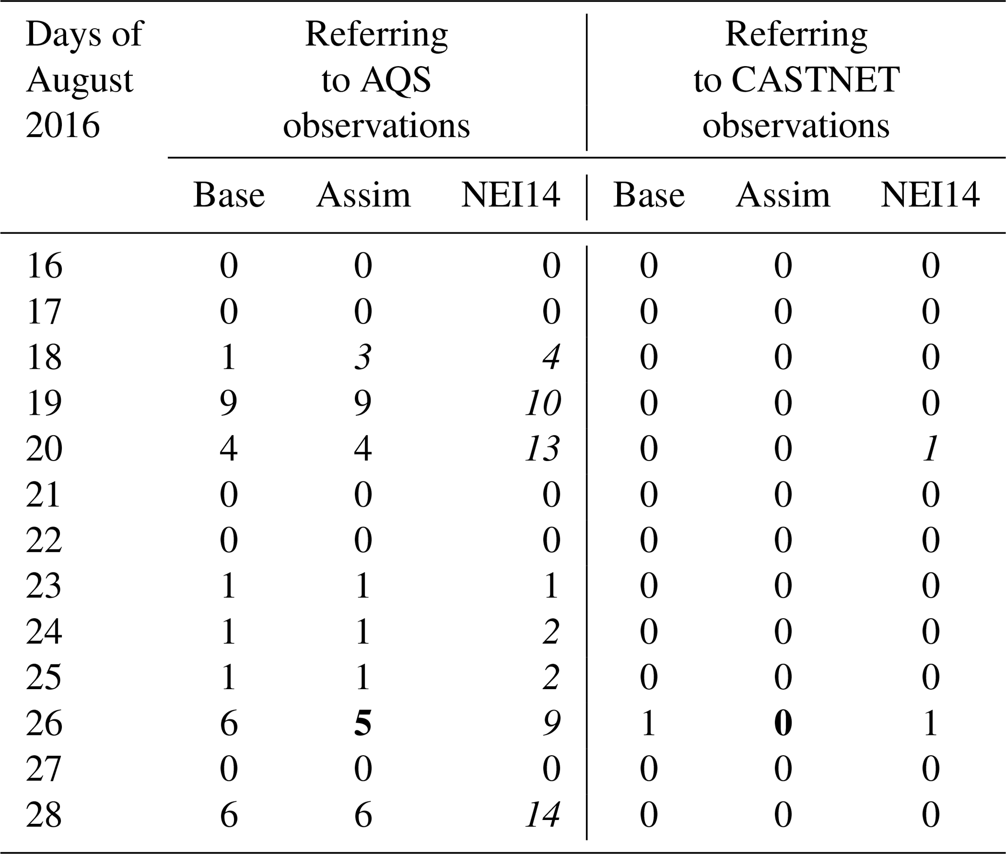
Acronyms: AQS: Air Quality System; CASTNET: Clean Air Status and Trends Network; MDA8: daily maximum 8 h average.
It is noticed that daytime surface O3 fields from the global CAMS and AM4 modeling systems are overall higher than those simulated by WRF-Chem (Fig. 10b; d; e). One of the reasons is that stratosphere–troposphere exchanges are better represented in these two global models. According to AM4's stratospheric tracer, during the study period, the stratospheric O3 influences on daytime surface O3 range from <2 ppbv in the Southern Great Plains (storm-affected regions) to 6–7 ppbv around Kansas and the Atlantic Ocean. Note that although AM4 provides a broad overview of the areas strongly impacted by stratospheric air, fine-scale features associated with stratospheric intrusions may be missing from this coarse-resolution simulation (Lin et al., 2012; Ott et al., 2016). Figure S7 (middle) indicates that the WRF-Chem modeling system used is capable of reproducing the downward and upward movements of pollutants; i.e., positive vertical wind speeds are shown over storm-active regions and negative vertical wind speeds over many regions that were strongly affected by stratospheric O3. However, as this modeling system only has tropospheric chemistry, the influences of stratospheric chemical compounds are represented only through the model's chemical lateral boundary conditions. This representation may be improved by adding accurate, time-varying chemical upper boundary conditions, e.g., downscaled from a fine-resolution (e.g., with horizontal spacing <50 km), well-performed global model simulation. Such an update, however, is expected to increase the modeled surface O3 (e.g., Fig. 3 in Huang et al., 2013, based on a different regional air quality model). For regions where modeled surface O3 is already positively biased, stronger efforts to address other sources of model errors would be needed to achieve desirable surface O3 performance.
3.3.2 Ozone at various altitudes
The SMAP DA impacts on WRF-Chem-modeled chemical fields are also investigated at a wide range of altitudes. Figure 7i–p compare the observed and WRF-Chem base case CO and O3 concentrations along nine ACT-America flights in August 2016, as well as the SMAP DA impacts on WRF-Chem results at these sampling locations. The observed and modeled CO vertical profiles show strong day-by-day variability, with near-surface concentrations ranging from 60 to 170 ppbv and elevated concentrations aloft (>90 ppbv at <600 hPa) occurring on 16, 20, and 21 August when aircraft measurements were taken under stormy weather conditions. In general, the observed and modeled O3 increase with altitude. WRF-Chem captured the magnitudes of the near-surface O3 concentrations fairly well but underpredicted O3 in the free troposphere. Overall, the modeled trace gas concentrations reacted to the SMAP DA most strongly near the surface. Under stormy weather conditions, the maximum changes in modeled CO and O3 approach 20 and 10 ppbv, respectively, corresponding to improved model performance at these locations (Fig. 7k–l; o–p). The SMAP DA impacts on modeled CO and O3 RMSEs are overall close to neutral ( %) but over 2 % during selected flights (Fig. 8b). Similar to the evaluation results for surface weather and O3 fields, the O3 performance changes by the SMAP DA are less desirable than those in the weather fields.
To help better understand SM controls on upper tropospheric O3 chemistry, Figs. 13d–i and S7 (lower) show the period-mean (16–28 August 2016) daytime O3, CO, NO2, and lightning NOx tracer results at ∼400 hPa from the WRF-Chem base simulation, as well as the SMAP DA impacts on these model fields. The daily daytime O3 responses to the SMAP DA at ∼400 hPa are presented in Fig. 11c. Elevated WRF-Chem O3 concentrations (>70 ppbv) are seen near the center of the upper tropospheric anticyclone (Fig. S2, right), which circulated the lifted pollutants and promoted in situ chemical production. The SMAP DA modified the period-mean daytime O3 by up to 1–1.5 ppbv, and its impacts on daytime O3 on individual days during the study period occasionally exceed 10 ppbv, which is larger than its maximum impact on the daily daytime surface O3 (Fig. 11a; c). As indicated by the modeled CO as well as NO2 and lightning NOx tracer responses to the SMAP DA, the O3 distributions in the upper troposphere and their responses to the SMAP DA are partially controlled by atmospheric transport and rapid in situ chemical production of O3 from lightning NO and other emissions, both of which are sensitive to SM. CO is used here primarily as a tracer of transport, but note that lightning and other emissions can modify CO lifetimes.

Figure 13Period-mean (16–28 August 2016) daytime O3 in the upper troposphere (i.e., the model levels close to 400 hPa) from (a) CAMS; (b) GFDL AM4; and (d) WRF-Chem base case. Panel (g) shows the impact of the SMAP DA on WRF-Chem-modeled daytime O3 in the upper troposphere, and panel (c) indicates the stratospheric influences on O3 at these altitudes based on the AM4 stratospheric O3 tracer output. Period-mean daytime CO and NO2 from WRF-Chem base case as well as their responses to the SMAP DA are shown in (e, h) and (f, i), respectively.
Similar to the O3 conditions at the surface, at ∼400 hPa, WRF-Chem daytime O3 concentrations are lower than the global CAMS and AM4 results (Fig. 13a–b) as well as the ACT-America aircraft measurements (Fig. 7m–n), by up to tens of parts per billion by volume. The AM4 stratospheric tracer suggests 5–17 ppbv of stratospheric influences on the period-mean O3 at these altitudes (Fig. 13c), which again helps identify the shortcomings of WRF-Chem in representing stratosphere–troposphere exchanges. Applying accurate, time-varying chemical upper boundary conditions in future works can help better assess the SMAP DA impact on O3 performance in the upper troposphere and improve the understanding of upper tropospheric chemistry.
To help interpret the SMAP DA impacts on various atmospheric processes such as vertical transport and lightning associated with convection and other phenomena, model results from the base and minus001 cases during two ACT-America flights were compared (Fig. S8). In the afternoon of 20 August 2016, the B-200 flew at <500 hPa over cold regions in Oklahoma and Arkansas affected by convection, with a cold front involved. On 27 August 2016 when most southeastern US regions were experiencing fair and warm weather, some of the B-200 measurements were collected at <400 hPa over southern Mississippi, influenced by deep convection. The WRF-Chem-modeled CO concentrations in the free troposphere above the regions affected by the cold front and/or convection are shown strongly sensitive to surface SM, and AM4 stratospheric O3 tracer output suggests enhanced stratospheric influences near the cold front and/or convection-affected locations. While this sensitivity analysis based on a constant surface SM perturbation helped confirm the SM impacts on atmospheric weather and chemistry, it is important to note that in reality the SM–atmosphere feedbacks are controlled by the magnitude and spatial heterogeneity of SM, which were both adjusted by the SMAP DA. Figure 7k–l show that the SMAP DA improved the WRF-Chem CO concentrations in the upper troposphere during both of these flights.
It is also noticed that the daytime O3 changes related to the anthropogenic emission update from NEI 2014 to NEI 2016 beta (<20 % of change for most species as introduced in Sect. 2.1) have comparable magnitudes with those due to the SMAP DA in the upper troposphere. For example, at ∼400 hPa, those changes are mostly within ±10 and ±1.5 ppbv at daily and 13 d timescales, respectively (Figs. 11c–d; 13g and S9, upper). This suggests that the SMAP DA and the US EPA-estimated anthropogenic emission change from 2014 to 2016 over the southeastern US could have similar levels of impacts on modeled O3 export from this region. The magnitudes of WRF-Chem upper tropospheric O3 sensitivities to anthropogenic emissions and SM are close to those based on archived global model sensitivity simulations for August 2010, which quantify monthly O3 responses to a constant 20 % reduction in North American anthropogenic emissions (i.e., 0.7–1.5 ppbv; Fig. S9, lower). These global model simulations also estimated that this 20 % emission reduction in North America affected O3 in other regions of the world; e.g., ∼400 hPa and surface O3 in Europe decreased by 0.4–0.7 and 0.1–0.5 ppbv, respectively (Fig. S9, lower–middle). Our WRF-Chem results, together with the findings from these past global model experiments, suggest that SM plays an important role in quantifying air pollutants' source–receptor relationships between the US and its downwind regions. It also emphasizes that using outdated anthropogenic emissions in WRF-Chem would lead to inaccurate assessments of the SMAP DA impacts on the model performance of O3 and other air pollutants over a broad region.
3.4 Evaluation of NEI 2014 using WRF-Chem simulations and SEAC4RS observations
We compared CO, NO2, and HCHO from two 25 km WRF-Chem simulations (i.e., SEACf and SEACa cases in Table 1) with aircraft observations during six SEAC4RS flights in August 2013 (Fig. S10). Such comparisons help evaluate the emissions of O3 precursors from various (e.g., NEI 2014 anthropogenic, lightning, and biogenic) sources as well as showing how the model representation of land–atmosphere interactions can affect such emission assessments. It is shown that in the SEACf case, WRF-Chem reproduced the overall vertical gradients of the observed chemicals, except that at this resolution it had difficulty in capturing urban plumes (e.g., for where the observed NO2>4 ppbv). This suggests that emissions of major O3 precursors are moderately well represented in the WRF-Chem system used. The strongest improvements in modeled CO, NO2, and HCHO by assimilating the CCI SM are ∼12, ∼0.6, and ∼1.2 ppbv, respectively, all occurring near the surface (>700 hPa). In the upper troposphere, the SM DA enhanced the modeled CO by up to ∼6 ppbv (at ∼200 hPa) and reduced the modeled NO2 by up to ∼0.5 ppbv (at ∼400 hPa). These changes led to better model agreements with the observations, indicating that assimilating the CCI SM likely improved the model treatment of lightning production and convective transport. As the SM DA modified the mismatches between the modeled and the observed trace gas concentrations, it is suggested that accurate representations of land–atmosphere interactions can benefit more rigorous evaluation and improvement of emissions using observations. Additionally, aircraft observations show robustness in aiding the evaluation of the emissions of O3 precursors from various sources, and therefore continuing to make rich and detailed observations like these would be helpful for evaluating and improving newer/future versions of emission estimates as well as the model representations of land–atmosphere interactions.
This study focused on evaluating SMAP SM DA impacts on coupled WRF-Chem weather and air quality modeling over the southeastern US during the ACT-America campaign in August 2016. The impacts of SMAP DA on WRF-Chem-modeled daytime RH as well as evaporative fraction were qualitatively consistent with the changes in the model's initial SM states, which were anti-correlated with the modeled daytime surface T2 and PBLH changes. The DA impacts on the model performance of SM, weather states, and energy fluxes showed strong spatiotemporal variability. Many factors may have impacted the effectiveness of the DA, including missing processes such as water use from human activities (e.g., irrigation), as well as dense vegetation and complex terrain, as also discussed in detail in our previous SMAP DA study. Referring to the gridded NCEP surface observations, the domain-wide mean RMSEs of modeled T2, RH, and WS were changed by the DA by ∼0 K, −0.024 %, and −0.005 m s−1, respectively. Referring to ACT-America aircraft observations on 9 flight days, the DA reduced the RMSEs of WRF-Chem air temperature and water vapor by ∼0.7 % and ∼2.3 %, respectively. The most significant improvements in the modeled air temperature and humidity occurred at ≥800 hPa, where their RMSEs were both reduced by ∼2.7 %. The overall DA impact on the modeled rainfall was less discernable, within the discrepancies between two rainfall evaluation products in places. The DA impacts on model performance were not consistent for energy flux partitioning and land–atmosphere states everywhere, suggesting that the modeling system used had shortcomings in representing SM–flux coupling and/or the relationships between moisture and heat fluxes and the atmospheric weather which need to be more clearly identified and corrected. Future efforts should focus on (1) applications using other LSMs and up-to-date inputs and parameters, along with multivariate land DA; (2) evaluation of additional water and energy flux variables (e.g., runoff, radiation); and (3) utilization of alternative LIS/WRF configurations, including adding irrigation processes to the modeling system and performing convection-permitting simulations with the assimilation of various kinds of high-resolution land products. Additionally, improving bias correction methods (e.g., also matching higher order moments of the LSM and satellite SM climatology) and practicing the assimilation of SMAP Level 1 brightness temperature alone or in combination with atmospheric observations will be needed.
The SMAP DA impact on WRF-Chem surface daytime-average and MDA8 O3 were strongly correlated with the changes in daytime T2 and PBLH, which were anti-correlated with the daytime surface humidity changes. The DA-induced surface O3 changes can largely be explained by the temperature-driven changes in biogenic emissions of VOCs and soil NO, chemical reaction rates, and dry deposition velocities. The SMAP DA impacts on WRF-Chem-modeled O3 along the ACT-America flight paths were particularly strong (i.e., approaching 10 ppbv at some ≥800 hPa locations) under stormy weather conditions. The WRF-Chem (near-)surface O3 performance change in response to the DA was overall less desirable than the changes in the weather fields; e.g., referring to gridded AQS and CASTNET O3 observations, the domain-wide mean MDA8 RMSEs increased by 0.057 and 0.007 ppbv, respectively. This was in part because many other factors also affected the model's surface O3 performance, such as shortcomings in model parameterizations (e.g., chemical mechanism, natural emission, photolysis and deposition schemes) and the model representations of anthropogenic emissions and stratosphere–troposphere exchanges.
We showed that at ∼400 hPa, elevated O3 concentrations were modeled near the center of the upper tropospheric anticyclone. The modeled O3 was negatively biased, mainly resulting from the poor representation of stratosphere–troposphere exchanges by WRF-Chem. The impact of SMAP DA on upper tropospheric O3 was partially via altering the transport of O3 and its precursors from other places as well as in situ chemical production of O3 from lightning NO and other emissions (including O3 precursors transported from elsewhere). Case studies of convection and/or cold-front-related events suggested that the DA improved the model treatment of convective transport and/or lightning production, which strengthened and extended the findings in Huang et al. (2018). We also showed that the impacts of DA and an emission update from NEI 2014 to NEI 2016 beta on WRF-Chem upper tropospheric O3 had comparable magnitudes. As reducing North American anthropogenic emissions would benefit the mitigation of O3 pollution in its downwind regions, our analysis highlighted the important role of SM in quantifying air pollutants' source–receptor relationships between the US and its downwind areas. It also emphasized that using up-to-date anthropogenic emissions in WRF-Chem would be necessary for accurately assessing SM DA impacts on the model performance of O3 and other air pollutants over a broad region. Continuing to improve NEI 2016 beta and any newer versions of emission estimates, as well as the parameterizations and other inputs of the models, is strongly encouraged. Such efforts can benefit from rich, detailed, high-accuracy observations, such as those taken during airborne field campaigns.
This study is a critical first step towards using satellite SM products to help improve the simulated weather and chemistry fields in models that are widely used for air quality research and forecasting, as well as policy-relevant assessments. It was demonstrated that, via changing the model's weather fields that drove its chemistry calculations online, the SM DA influenced various O3-related processes, O3 concentrations, and O3 exceedances modeled by WRF-Chem. In some locations/times, these influences were significant and resulted in improved model performance. To further improve the modeled chemical fields via applying the SM DA at various scales, it is not only important to improve the model representations of anthropogenic emissions and trans-boundary transport, but also to address shortcomings in model parameterizations, e.g., to realistically reflect the impacts of water availability on biogenic emissions and dry deposition, and for longer simulations, to include O3 damage to vegetation (e.g., Hudman et al., 2012; Val Martin et al., 2014; Sadiq et al., 2017; Jiang et al., 2018; Clifton et al., 2020). Using dynamic vegetation models (available in the Noah-Multiparameterization LSM) along with additional process-based (e.g., chemical fluxes, stomatal behaviors) measurements and laboratory experiments would be necessary for improving some of these parameterizations, and these will be experimented in a follow-up study. Community efforts such as the ongoing Air Quality Model Evaluation International Initiative Phase 4 experiment (https://aqmeii.jrc.ec.europa.eu/phase4.html, last access: 14 March 2021) would also be greatly beneficial. High-quality weather input is a requirement for rigorous evaluations of any set of these parameterizations.
The stand-alone LIS is accessible at https://lis.gsfc.nasa.gov/source (NASA, 2016, last access: 27 March 2020). LIS/WRF-Chem coupling is facilitated in the NASA-Unified WRF system (NASA, 2019, https://nuwrf.gsfc.nasa.gov/software, last access: 27 March 2020). The global C-IFS simulations for HTAP phase 2 can be downloaded from the AeroCom database following guidelines at http://iek8wikis.iek.fz-juelich.de/HTAPWiki/HTAP-2-data-submission (HTAPWiki, 2016, last access: 16 June 2021). Observations and observation-derived data products used in this work can be found at the following locations: https://doi.org/10.5067/RFKIZ5QY5ABN (O'Neill et al., 2018), https://www.geo.tuwien.ac.at/insitu/data_viewer (Vienna University of Technology, 2021, last access: 22 February 2021), https://www.esa-soilmoisture-cci.org/data (ESA, 2019, last access: 25 October 2019), https://www-air.larc.nasa.gov/cgi-bin/ArcView/actamerica.2016 (NASA, 2020, last access: 7 November 2020), https://doi.org/10.5067/Aircraft/SEAC4RS/Aerosol-TraceGas-Cloud (NASA, 2018), https://aqs.epa.gov/aqsweb/airdata/download_files.html (US EPA, 2019a, last access: 6 March 2020), https://java.epa.gov/castnet/clearsession.do (US EPA, 2019b, last access: 30 May 2019), https://doi.org/10.5065/4F4P-E398 (NCEP, 2004), https://doi.org/10.17190/AMF/1436327 (Billesbach et al., 2018a), https://doi.org/10.17190/AMF/1436328 (Billesbach et al., 2018b), https://doi.org/10.17190/AMF/1246027 (Biraud et al., 2020), https://doi.org/10.17190/AMF/1246132 (Brunsell, 2020), https://doi.org/10.17190/AMF/1498745 (Brunsell, 2019), https://doi.org/10.17190/AMF/1246080 (Novick and Phillips, 2021), https://doi.org/10.17190/AMF/1246081 (Wood and Gu, 2019), https://doi.org/10.17190/AMF/1246083 (Noormets, 2021), https://doi.org/10.17190/AMF/1419506 (Noormets, 2020), http://www.fluxcom.org/EF-Download/ (Max Planck Institute for Biogeochemistry, 2019, last access: 22 January 2020), https://doi.org/10.5065/D6PG1QDD (Du, 2011), and https://doi.org/10.5067/GPM/IMERG/3B-HH/06 (Huffman et al., 2019b).
The supplement related to this article is available online at: https://doi.org/10.5194/acp-21-11013-2021-supplement.
MH led the design and execution of the study, as well as the writing of the paper. JHC, JPD, GRC, and KWB contributed to the field campaign data collection and/or analysis. GRC, KWB, SVK, and XZ contributed to the modeling and/or DA work. All authors helped finalize the paper.
The authors declare that they have no conflict of interest.
We thank the ACT-America flight, instrument, and data management teams and the principal investigator of ACT-America, Kenneth Davis (Penn State), for designing and conducting the NASA B-200 flights, as well as helping with the analysis. We also thank the SEAC4RS instrument teams (PIs: Thomas Ryerson, NOAA/ESRL; Ronald Cohen, UC Berkeley; Alan Fried, CU-Boulder; Thomas Hanisco, NASA GSFC; Glenn Diskin, NASA LaRC; and Armin Wisthaler, University of Innsbruck) and FLUXNET PIs for sharing their measurements. The ECMWF CAMS and GFDL AM4 (contacts: Meiyun Lin, Princeton; Alex Zhang, now at Penn State) modeling teams are acknowledged for generating the global model outputs used in this study. The global C-IFS simulations for HTAP phase 2 were conducted by Johannes Flemming (ECMWF). Sophia Walther (MPI-BGC), Kazuyuki Miyazaki (JPL/Caltech), and Li Fang (UMD) provided datasets that are not directly related to this study but were informative. NASA's high-end computing systems and services are acknowledged.
This research has been supported by NASA’s Earth Science Division, through the Science Utilization of SMAP program (grant no. NNX16AN39G) and the Earth Venture Suborbital-2 ACT-America project (grant no. NNX15AG76G to Penn State).
This paper was edited by Rolf Müller and reviewed by two anonymous referees.
Anav, A., Proietti, C., Menut, L., Carnicelli, S., De Marco, A., and Paoletti, E.: Sensitivity of stomatal conductance to soil moisture: implications for tropospheric ozone, Atmos. Chem. Phys., 18, 5747–5763, https://doi.org/10.5194/acp-18-5747-2018, 2018.
Avnery, S., Mauzerall, D. L., Liu, J., and Horowitz, L. W.: Global Crop Yield Reductions due to Surface Ozone Exposure: 1. Year 2000 Crop Production Losses and Economic Damage, Atmos. Environ., 45, 2284–2296, https://doi.org/10.1016/j.atmosenv.2010.11.045, 2011.
Barth, M. C., Lee, J., Hodzic, A., Pfister, G., Skamarock, W. C., Worden, J., Wong, J., and Noone, D.: Thunderstorms and upper troposphere chemistry during the early stages of the 2006 North American Monsoon, Atmos. Chem. Phys., 12, 11003–11026, https://doi.org/10.5194/acp-12-11003-2012, 2012.
Baublitz, C. B., Fiore, A. M., Clifton, O. E., Mao, J., Li, J., Correa, G., Westervelt, D. M., Horowitz, L. W., Paulot, F., and Williams, A. P.: Sensitivity of Tropospheric Ozone Over the Southeast USA to Dry Deposition, Geophys. Res. Lett., 47, e2020GL087158, https://doi.org/10.1029/2020GL087158, 2020.
Bertschi, I. T. and Jaffe, D. A.: Long-range transport of ozone, carbon monoxide, and aerosols to the NE Pacific troposphere during the summer of 2003: Observations of smoke plumes from Asian boreal fires, J. Geophys. Res.-Atmos., 110, D05303, https://doi.org/10.1029/2004JD005135, 2005.
Betts, R. A., Ball, J. H., Beljaars, A. C. M., Miller, M. J., and Viterbo, P.: The land-surface-atmosphere interaction: A review based on observational and global modeling perspectives, J. Geophys. Res.-Atmos., 101, 7209–7225, https://doi.org/10.1029/95JD02135, 1996.
Billesbach, D., Kueppers, L., Torn, M., and Biraud, S.: AmeriFlux US-A32 ARM-SGP Medford hay pasture, Version 1-5, AmeriFlux AMP [data set], https://doi.org/10.17190/AMF/1436327, 2018a.
Billesbach, D., Kueppers, L., Torn, M., and Biraud, S.: AmeriFlux US-A74 ARM SGP milo field, Version 1-5, AmeriFlux AMP [data set], https://doi.org/10.17190/AMF/1436328, 2018b.
Biraud, S., Fischer, M., Chan, S., and Torn, M.: AmeriFlux US-ARM ARM Southern Great Plains site-Lamont, Version 10-5, AmeriFlux AMP [data set], https://doi.org/10.17190/AMF/1246027, 2020.
Boccippio, D. J., Cummins, K. L., Christian, H. J., and Goodman, S. J.: Combined Satellite- and Surface-Based Estimation of the Intracloud-Cloud-to-Ground Lightning Ratio over the Continental United States, Mon. Weather Rev., 129, 108–122, https://doi.org/10.1175/1520-0493(2001)129<0108:CSASBE>2.0.CO;2, 2001.
Bonn, B., Magh, R.-K., Rombach, J., and Kreuzwieser, J.: Biogenic isoprenoid emissions under drought stress: different responses for isoprene and terpenes, Biogeosciences, 16, 4627–4645, https://doi.org/10.5194/bg-16-4627-2019, 2019.
Bowman, K. W., Shindell, D. T., Worden, H. M., Lamarque, J. F., Young, P. J., Stevenson, D. S., Qu, Z., de la Torre, M., Bergmann, D., Cameron-Smith, P. J., Collins, W. J., Doherty, R., Dalsøren, S. B., Faluvegi, G., Folberth, G., Horowitz, L. W., Josse, B. M., Lee, Y. H., MacKenzie, I. A., Myhre, G., Nagashima, T., Naik, V., Plummer, D. A., Rumbold, S. T., Skeie, R. B., Strode, S. A., Sudo, K., Szopa, S., Voulgarakis, A., Zeng, G., Kulawik, S. S., Aghedo, A. M., and Worden, J. R.: Evaluation of ACCMIP outgoing longwave radiation from tropospheric ozone using TES satellite observations, Atmos. Chem. Phys., 13, 4057–4072, https://doi.org/10.5194/acp-13-4057-2013, 2013.
Brown-Steiner, B. and Hess, P.: Asian influence on surface ozone in the United States: A comparison of chemistry, seasonality, and transport mechanisms, J. Geophys. Res.-Atmos., 116, D17309, https://doi.org/10.1029/2011JD015846, 2011.
Brunsell, N.: AmeriFlux US-KLS Kansas Land Institute, Version 1-5, AmeriFlux AMP [data set], https://doi.org/10.17190/AMF/1498745, 2019.
Brunsell, N.: AmeriFlux US-KFS Kansas Field Station, Version 7-5, AmeriFlux AMP [data set], https://doi.org/10.17190/AMF/1246132, 2020.
Bucsela, E., Pickering, K. E., Allen, D. J., Holzworth, R. H., and Krotkov, N. A.: Mid-latitude lightning NOx production efficiency inferred from OMI and WWLLN data, J. Geophys. Res.-Atmos., 124, 13475–13497, https://doi.org/10.1029/2019JD030561, 2019.
Camalier, L., Cox, W., and Dolwick, P.: The effects of meteorology on ozone in urban areas and their use in assessing ozone trends, Atmos. Environ., 41, 7127–7137, https://doi.org/10.1016/j.atmosenv.2007.04.061, 2007.
Charusombat, U., Niyogi, D., Kumar, A., Wang, X., Chen, F., Guenther, A., Turnipseed, A., and Alapaty, K.: Evaluating a new deposition velocity module in the Noah land-surface model, Bound.-Lay. Meteorol., 137, 271–290, 2010.
Chen, F. and Dudhia, J.: Coupling an advanced land surface hydrology model with the Penn State-NCAR MM5 modeling system, Part I: Model implementation and sensitivity, Mon. Weather Rev., 129, 569–585, https://doi.org/10.1175/1520-0493(2001)129<0569:CAALSH>2.0.CO;2, 2001.
Cioni, G. and Hohenegger, C.: Effect of soil moisture on diurnal convection and precipitation in Large-Eddy Simulations, J. Hydrometeorol., 18, 1885–1903, https://doi.org/10.1175/JHMD-16-0241.1, 2017.
Clifton, O. E., Paulot, F., Fiore, A. M., Horowitz, L. W., Correa, G., Baublitz, C. B., Fares, S., Goded, I., Goldstein, A. H., Gruening, C., Hogg, A. J., Loubet, B., Mammarella, I., Munger, J. W., Neil, L., Stella, P., Uddling, J., Vesala, T., and Weng, E.: Influence of dynamic ozone dry deposition on ozone pollution, J. Geophys. Res.-Atmos., 125, e2020JD032398, https://doi.org/10.1029/2020JD032398, 2020.
Coates, J., Mar, K. A., Ojha, N., and Butler, T. M.: The influence of temperature on ozone production under varying NOx conditions – a modelling study, Atmos. Chem. Phys., 16, 11601–11615, https://doi.org/10.5194/acp-16-11601-2016, 2016.
Cohen, A. J., Brauer, M., Burnett, R., Anderson, H. R., Frostad, J., Estep, K., Balakrishnan, K., Brunekreef, B., Dandona, L., Dandona, R., Feigin, V., Freedman, G., Hubbell, B., Jobling, A., Kan, H., Knibbs, L., Liu, Y., Martin, R., Morawska, L., Pope, C. A., Shin, H., Straif, K., Shaddick, G., Thomas, M., van Dingenen, R., van Donkelaar, A., Vos, T., Murray, C. J. L., and Forouzanfar, M. H.: Estimates and 25-year trends of the global burden of disease attributable to ambient air pollution: an analysis of data from the Global Burden of Diseases Study 2015, Lancet, 389, 1907–1918, https://doi.org/10.1016/S0140-6736(17)30505-6, 2017.
Collow, T. W., Robock, A., and Wu, W.: Influences of soil moisture and vegetation on convective precipitation forecasts over the United States Great Plains, J. Geophys. Res.-Atmos., 119, 9338–9358, https://doi.org/10.1002/2014JD021454, 2014.
Cooper, O. R., Trainer, M., Thompson, A. M., Witte, J. C., Oltmans, S. J., Morris, G., Pickering, K. E., Crawford, J. H., Chen, G., Cohen, R. C., Bertram, T. H., Wooldridge, P., Perring, A., Brune, W. H., Merrill, J., Moody, J. L., Tarasick, D., Nédélec, P., Forbes, G., Newchurch, M. J., Schmidlin, F. J., Johnson, B. J., Turquety, S., Baughcum, S. L., Ren, X., Fehsenfeld, F. C., Meagher, J. F., Spichtinger, N., Brown, C. C., McKeen, S. A., McDermid, I. S., and Leblanc, T.: Large upper tropospheric ozone enhancements above midlatitude North America during summer: In situ evidence from the IONS and MOZAIC ozone measurement network, J. Geophys. Res.-Atmos., 111, D24S05, https://doi.org/10.1029/2006JD007306, 2006.
Cooper, O. R., Trainer, M., Thompson, A. M., Oltmans, S. J., Tarasick, D. W., Witte, J. C., Stohl, A., Eckhardt, S., Lelieveld, J., Newchurch, M. J., Johnson, B. J., Portmann, R. W., Kalnajs, L., Dubey, M. K., Leblanc, T., McDermid, I. S., Forbes, G., Wolfe, D., Carey-Smith, T., Morris, G. A., Lefer, B., Rappenglück, B., Joseph, E., Schmidlin, F., Meagher, J., Fehsenfeld, F. C., Keating, T. J., Van Curen, R. A., and Minschwaner, K.: Evidence for a recurring eastern North America upper tropospheric ozone maximum during summer, J. Geophys. Res.-Atmos., 112, D23304, https://doi.org/10.1029/2007JD008710, 2007.
Cooper, O. R., Eckhardt, S., Crawford, J. H., Brown, C. C., Cohen, R. C., Bertram, T. H., Wooldridge, P., Perring, A., Brune, W. H., Ren, X., Brunner, D., and Baughcum, S. L.: Summertime buildup and decay of lightning NOx and aged thunderstorm outflow above North America, J. Geophys. Res.-Atmos., 114, D01101, https://doi.org/10.1029/2008JD010293, 2009.
Cooper, O. R., Parrish, D. D., Ziemke, J., Balashov, N. V., Cupeiro, M., Galbally, I. E., Gilge, S., Horowitz, L., Jensen, N. R., Lamarque, J.-F., Naik, V., Oltmans, S. J., Schwab, J., Shindell, D. T., Thompson, A. M., Thouret, V., Wang, Y., and Zbinden, R. M.: Global distribution and trends of tropospheric ozone: An observation-based review, Elem. Sci. Anth., 2, 000029, https://doi.org/10.12952/journal.elementa.000029, 2014.
Darmenov, A. and da Silva, A.: The Quick Fire Emissions Dataset (QFED): Documentation of versions 2.1, 2.2 and 2.4, NASA Technical Report Series, Global Modeling and Data Assimilation, NASA TM-2015-104606/Volume 38, available at: http://gmao.gsfc.nasa.gov/pubs/docs/Darmenov796.pdf (last access: 27 March 2020), 2015.
de Rosnay, P., Drusch, M., Vasiljevic, D., Balsamo, G., Albergel, C., and Isaksen, L.: A simplified Extended Kalman Filter for the global operational soil moisture analysis at ECMWF, Q. J. Roy. Meteor. Soc., 139, 1199–1213, https://doi.org/10.1002/qj.2023, 2013.
Dickerson, R. R., Huffman, G. L., Luke, W. T., Nunnermacker, L. J., Pickering, K. E., Leslie, A. C., Lindsey, C. G., Slinn, W. G. N., Kelly, T. J., Daum, P. H., Delany, A. C., Greenberg, J. P., Zimmerman, P. R., Boatman, J. F., Ray, J. D., and Stedman, D. H.: Thunderstorms – An important mechanism in the transport of air pollutants, Science, 235, 460–464, https://doi.org/10.1126/science.235.4787.460, 1987.
Dirmeyer, P. A.: The terrestrial segment of soil moisture-climate coupling, Geophys. Res. Lett., 38, L16702, https://doi.org/10.1029/2011GL048268, 2011.
Dirmeyer, P. A., Cash, B. A., Kinter III, J. L., Jung, T., Marx, L., Satoh, M., Stan, C., Tomita, H., Towers, P., Wedi, N., Achuthavarier, D., Adams, J. M., Altshuler, E. L., Huang, B., Jin, E. K., and Manganello, J.: Simulating the diurnal cycle of rainfall in global climate models: resolution versus parameterization, Clim. Dynam., 39, 399–418, https://doi.org/10.1007/s00382-011-1127-9, 2012.
Dirmeyer, P. A., Jin, Y., Singh, B., and Yan, X.: Evolving land-atmosphere interactions over North America from CMIP5 simulations, J. Climate, 26, 7313–7327, https://doi.org/10.1175/JCLI-D-12-00454.1, 2013.
Doherty, R. M.: Ozone Pollution from Near and Far, Nat. Geosci., 8, 664–665, https://doi.org/10.1038/ngeo2497, 2015.
Doherty, R. M., Wild, O., Shindell, D. T., Zeng, G., MacKenzie, I. A., Collins, W. J., Fiore, A. M., Stevenson, D. S., Dentener, F. J., Schultz, M. G., Hess, P., Derwent, R. G., and Keating, T. J.: Impacts of climate change on surface ozone and intercontinental ozone pollution: A multi-model study, J. Geophys. Res.-Atmos., 118, 3744–3763, https://doi.org/10.1002/jgrd.50266, 2013.
Dorigo, W. A., Wagner, W., Hohensinn, R., Hahn, S., Paulik, C., Xaver, A., Gruber, A., Drusch, M., Mecklenburg, S., van Oevelen, P., Robock, A., and Jackson, T.: The International Soil Moisture Network: a data hosting facility for global in situ soil moisture measurements, Hydrol. Earth Syst. Sci., 15, 1675–1698, https://doi.org/10.5194/hess-15-1675-2011, 2011.
Du, J.: GCIP/EOP Surface: Precipitation NCEP/EMC 4KM Gridded Data (GRIB) Stage IV Data, Version 1.0, UCAR/NCAR – Earth Observing Laboratory [data set], Boulder, Colorado, USA, https://doi.org/10.5065/D6PG1QDD, 2011.
Entekhabi, D., Njoku, E. G., O'Neill, P. E., Kellogg, K. H., Crow, W. T., Edelstein, W. N., Entin, J. K., Goodman, S. D., Jackson, T. J., Johnson, J., Kimball, J., Piepmeier, J. R., Koster, R. D., Martin, N., McDonald, K. C., Moghaddam, M., Moran, S., Reichle, R., Shi, J. C., Spencer, M. W., Thurman, S. W., Tsang, L., and van Zyl, J.: The Soil Moisture Active Passive (SMAP) Mission, Proc. IEEE, 98, 704–716, https://doi.org/10.1109/JPROC.2010.2043918, 2010.
ESA: ESA CCI Soil Moisture Data, Version 04.5, Vienna University of Technology SFTP site [data set], Vienna, Austria, available at: https://www.esa-soilmoisture-cci.org/data, last access: 25 October 2019.
Fast, J. D., Berg, L. K., Feng, Z., Mei, F., Newsom, R., Sakaguchi, K., and Xiao, H.: The impact of variable land-atmosphere coupling on convective cloud populations observed during the 2016 HI-SCALE field campaign, J. Adv. Model. Earth Sy., 11, 2629–2654, https://doi.org/10.1029/2019MS001727, 2019.
Finney, D. L., Doherty, R. M., Wild, O., Stevenson, D. S., Mackenzie, I. A., and Blyth, A.: A projected decrease in lightning under climate change, Nat. Clim. Change, 8, 210–213, https://doi.org/10.1038/s41558-018-0072-6, 2018.
Fiore, A. M., Dentener, F. J., Wild, O., Cuvelier, C., Schultz, M. G., Hess, P., Textor, C., Schulz, M., Doherty, R. M., Horowitz, L. W., MacKenzie, I. A., Sanderson, M. G., Shindell, D. T., Stevenson, D. S., Szopa, S., Van Dingenen, R., Zeng, G., Atherton, C., Bergmann, D., Bey, I., Carmichael, G., Collins, W. J., Duncan, B. N., Faluvegi, G., Folberth, G., Gauss, M., Gong, S., Hauglustaine, D., Holloway, T., Isaksen, I. S. A., Jacob, D. J., Jonson, J. E., Kaminski, J. W., Keating, T. J., Lupu, A., Marmer, E., Montanaro, V., Park, R. J., Pitari, G., Pringle, K. J., Pyle, J. A., Schroeder, S., Vivanco, M. G., Wind, P., Wojcik, G., Wu, S., and Zuber, A.: Multimodel estimates of intercontinental source receptor relationships for ozone pollution, J. Geophys. Res.-Atmos., 114, D04301, https://doi.org/10.1029/2008JD010816, 2009.
Fishman, J., Belina, K. M., and Encarnación, C. H.: The St. Louis Ozone Gardens: Visualizing the Impact of a Changing Atmosphere, B. Am. Meteorol. Soc., 95, 1171–1176, https://doi.org/10.1175/bams-d-13-00009.1, 2014.
Fleming, Z. L., Doherty, R. M., von Schneidemesser, E., Malley, C. S., Cooper, O. R., Pinto, J. P., Colette, A., Xu, X., Simpson, D., Schultz, M. G., Lefohn, A. S., Hamad, S., Moolla, R., Solberg, S., and Feng, Z.: Tropospheric Ozone Assessment Report: Present-day ozone distribution and trends relevant to human health, Elem. Sci. Anth., 6, 12, https://doi.org/10.1525/elementa.273, 2018.
Gevaert, A. I., Miralles, D. G., de Jeu, R. A. M., Schellekens, J., and Dolman, A. J.: Soil moisture-temperature coupling in a set of land surface models, J. Geophys. Res.-Atmos., 123, 1481–1498, https://doi.org/10.1002/2017JD027346, 2018.
Grell, G. A. and Freitas, S. R.: A scale and aerosol aware stochastic convective parameterization for weather and air quality modeling, Atmos. Chem. Phys., 14, 5233–5250, https://doi.org/10.5194/acp-14-5233-2014, 2014.
Grell, G. A., Peckham, S., Schmitz, R., McKeen, S., Frost, G., Skamarock, W., and Eder, B.: Fully coupled “online” chemistry within the WRF model, Atmos. Environ., 39, 6957–6976, https://doi.org/10.1016/j.atmosenv.2005.04.027, 2005.
Gruber, A., Scanlon, T., van der Schalie, R., Wagner, W., and Dorigo, W.: Evolution of the ESA CCI Soil Moisture climate data records and their underlying merging methodology, Earth Syst. Sci. Data, 11, 717–739, https://doi.org/10.5194/essd-11-717-2019, 2019.
Guenther, A., Karl, T., Harley, P., Wiedinmyer, C., Palmer, P. I., and Geron, C.: Estimates of global terrestrial isoprene emissions using MEGAN (Model of Emissions of Gases and Aerosols from Nature), Atmos. Chem. Phys., 6, 3181–3210, https://doi.org/10.5194/acp-6-3181-2006, 2006.
Guenther, A. B., Jiang, X., Heald, C. L., Sakulyanontvittaya, T., Duhl, T., Emmons, L. K., and Wang, X.: The Model of Emissions of Gases and Aerosols from Nature version 2.1 (MEGAN2.1): an extended and updated framework for modeling biogenic emissions, Geosci. Model Dev., 5, 1471–1492, https://doi.org/10.5194/gmd-5-1471-2012, 2012.
Guillod, B. P., Orlowsky, B., Miralles, D. G., Teuling, A. J., and Seneviratne, S. I.: Reconciling spatial and temporal soil moisture effects on afternoon rainfall, Nat. Commun., 6, 6443, https://doi.org/10.1038/ncomms7443, 2015.
Guo, Z. and Dirmeyer, P. A.: Interannual variability of land-atmosphere coupling strength, J. Hydrometeorol., 14, 1636–1646, https://doi.org/10.1175/JHM-D-12-0171.1, 2013.
Harlan, S. L. and Ruddell, D. M.: Climate change and health in cities: impacts of heat and air pollution and potential co-benefits from mitigation and adaptation, Curr. Opin. Env. Sust., 3, 126–134, https://doi.org/10.1016/j.cosust.2011.01.001, 2011.
Harris, N. R. P., Hassler, B., Tummon, F., Bodeker, G. E., Hubert, D., Petropavlovskikh, I., Steinbrecht, W., Anderson, J., Bhartia, P. K., Boone, C. D., Bourassa, A., Davis, S. M., Degenstein, D., Delcloo, A., Frith, S. M., Froidevaux, L., Godin-Beekmann, S., Jones, N., Kurylo, M. J., Kyrölä, E., Laine, M., Leblanc, S. T., Lambert, J.-C., Liley, B., Mahieu, E., Maycock, A., de Mazière, M., Parrish, A., Querel, R., Rosenlof, K. H., Roth, C., Sioris, C., Staehelin, J., Stolarski, R. S., Stübi, R., Tamminen, J., Vigouroux, C., Walker, K. A., Wang, H. J., Wild, J., and Zawodny, J. M.: Past changes in the vertical distribution of ozone – Part 3: Analysis and interpretation of trends, Atmos. Chem. Phys., 15, 9965–9982, https://doi.org/10.5194/acp-15-9965-2015, 2015.
Hemispheric Transport of Air Pollution (HTAP): 2010 Final Assessment report, Part A: Ozone and particulate matter, available at: http://htapold.kaskada.tk/publications/2010_report/2010_Final_Report/HTAP 2010 Part A 110407.pdf, (last access: 16 June 2021), 2010.
Hess, P. G.: A comparison of two paradigms: The relative global roles of moist convective versus nonconvective transport, J. Geophys. Res.-Atmos., 110, D20302, https://doi.org/10.1029/2004JD005456, 2005.
Hogrefe, C., Isukapalli, S., Tang, X., Georgopoulos, P., He, S., Zalewsky, E., Hao, W., Ku, J., Key, T., and Sistla, G.: Impact of biogenic emission uncertainties on the simulated response of ozone and fine particulate matter to anthropogenic emission reductions, J. Air Waste Manage., 61, 92–108, https://doi.org/10.3155/1047-3289.61.1.92, 2011.
Hohenegger, C., Brockhaus, P., Bretherton, C. S., and Schär, C.: The soil moisture-precipitation feedback in simulations with explicit and parameterized convection, J. Climate, 22, 5003–5020, https://doi.org/10.1175/2009JCLI2604.1, 2009.
Horowitz, L. W., Naik, V., Paulot, F., Ginoux, P. A., Dunne, J. P., Mao, J., Schnell, J., Chen, X., He, J., Lin, M., Lin, P., Malyshev, S. P. D., Shevliakova, E., and Zhao, M.: The GFDL Global Atmospheric Chemistry-Climate Model AM4.1: Model Description and Simulation Characteristics, J. Adv. Model. Earth Sy., 12, e2019MS002032, https://doi.org/10.1029/2019MS002032, 2020.
HTAPWiki: HTAP phase 2/AeroCom data submission requirements, available at: http://iek8wikis.iek.fz-juelich.de/HTAPWiki/HTAP-2-data-submission (last access: 16 June 2021), 2016.
Huang, M., Carmichael, G. R., Adhikary, B., Spak, S. N., Kulkarni, S., Cheng, Y. F., Wei, C., Tang, Y., Parrish, D. D., Oltmans, S. J., D'Allura, A., Kaduwela, A., Cai, C., Weinheimer, A. J., Wong, M., Pierce, R. B., Al-Saadi, J. A., Streets, D. G., and Zhang, Q.: Impacts of transported background ozone on California air quality during the ARCTAS-CARB period – a multi-scale modeling study, Atmos. Chem. Phys., 10, 6947–6968, https://doi.org/10.5194/acp-10-6947-2010, 2010.
Huang, M., Carmichael, G. R., Chai, T., Pierce, R. B., Oltmans, S. J., Jaffe, D. A., Bowman, K. W., Kaduwela, A., Cai, C., Spak, S. N., Weinheimer, A. J., Huey, L. G., and Diskin, G. S.: Impacts of transported background pollutants on summertime western US air quality: model evaluation, sensitivity analysis and data assimilation, Atmos. Chem. Phys., 13, 359–391, https://doi.org/10.5194/acp-13-359-2013, 2013.
Huang, M., Lee, P., McNider, R., Crawford, J., Buzay, E., Barrick, J., Liu, Y., and Krishnan, P.: Temporal and spatial variability of daytime land surface temperature in Houston: Comparing DISCOVER-AQ aircraft observations with the WRF model and satellites, J. Geophys. Res.-Atmos., 121, 185–195, https://doi.org/10.1002/2015JD023996, 2016.
Huang, M., Carmichael, G. R., Pierce, R. B., Jo, D. S., Park, R. J., Flemming, J., Emmons, L. K., Bowman, K. W., Henze, D. K., Davila, Y., Sudo, K., Jonson, J. E., Tronstad Lund, M., Janssens-Maenhout, G., Dentener, F. J., Keating, T. J., Oetjen, H., and Payne, V. H.: Impact of intercontinental pollution transport on North American ozone air pollution: an HTAP phase 2 multi-model study, Atmos. Chem. Phys., 17, 5721–5750, https://doi.org/10.5194/acp-17-5721-2017, 2017a.
Huang, M., Carmichael, G. R., Crawford, J. H., Wisthaler, A., Zhan, X., Hain, C. R., Lee, P., and Guenther, A. B.: Biogenic isoprene emissions driven by regional weather predictions using different initialization methods: case studies during the SEAC4RS and DISCOVER-AQ airborne campaigns, Geosci. Model Dev., 10, 3085–3104, https://doi.org/10.5194/gmd-10-3085-2017, 2017b.
Huang, M., Crawford, J. H., Diskin, G. S., Santanello, J. A., Kumar, S. V., Pusede, S. E., Parrington, M., and Carmichael, G. R.: Modeling regional pollution transport events during KORUS-AQ: Progress and challenges in improving representation of land-atmosphere feedbacks, J. Geophys. Res.-Atmos., 123, 10732–10756, https://doi.org/10.1029/2018JD028554, 2018.
Hudman, R. C., Russell, A. R., Valin, L. C., and Cohen, R. C.: Interannual variability in soil nitric oxide emissions over the United States as viewed from space, Atmos. Chem. Phys., 10, 9943–9952, https://doi.org/10.5194/acp-10-9943-2010, 2010.
Hudman, R. C., Moore, N. E., Mebust, A. K., Martin, R. V., Russell, A. R., Valin, L. C., and Cohen, R. C.: Steps towards a mechanistic model of global soil nitric oxide emissions: implementation and space based-constraints, Atmos. Chem. Phys., 12, 7779–7795, https://doi.org/10.5194/acp-12-7779-2012, 2012.
Huffman, G. J., Bolvin, D. T., Braithwaite, D., Hsu, K., Joyce, R., Kidd, C., Nelkin, E. J., Sorooshian, S., Tan, J., and Xie, P.: NASA Global Precipitation Measurement (GPM) Integrated Multi-satellitE Retrievals for GPM (IMERG), Algorithm Theoretical Basis Document (ATBD), Version 06, available at: https://pmm.nasa.gov/sites/default/files/document_files/IMERG_ATBD_V06.pdf (last access: 27 March 2020), 2019a.
Huffman, G. J., Stocker, E. F., Bolvin, D. T., Nelkin, E. J., and Tan, J.: GPM IMERG Final Precipitation L3 Half Hourly 0.1 degree x 0.1 degree V06, Goddard Earth Sciences Data and Information Services Center (GES DISC) [data set], Greenbelt, Maryland, USA, https://doi.org/10.5067/GPM/IMERG/3B-HH/06, 2019b.
Huijnen, V., Miyazaki, K., Flemming, J., Inness, A., Sekiya, T., and Schultz, M. G.: An intercomparison of tropospheric ozone reanalysis products from CAMS, CAMS interim, TCR-1, and TCR-2, Geosci. Model Dev., 13, 1513–1544, https://doi.org/10.5194/gmd-13-1513-2020, 2020.
Iacono, M. J., Delamere, J. S., Mlawer, E. J., Shephard, M. W., Clough, S. A., and Collins, W. D.: Radiative forcing by long-lived greenhouse gases: Calculations with the AER radiative transfer models, J. Geophys. Res.-Atmos., 113, D13103, https://doi.org/10.1029/2008JD009944, 2008.
Intergovernmental Panel on Climate Change: Climate Change 2013: The Physical Science Basis, in: Contribution of Working Group I to the Fifth Assessment Report of the Intergovernmental Panel on Climate Change, edited by: Stocker, T. F., Qin, D., Plattner, G.-K., Tignor, M., Allen, S. K., Boschung, J., Nauels, A., Xia, Y., Bex, V., and Midgley, P. M., Cambridge University Press, Cambridge, UK, New York, USA, available at: https://www.ipcc.ch/report/ar5/wg1 (last access: 27 March 2020), 2013.
Jacob, D. and Winner, D. A.: Effect of climate change on air quality, Atmos. Environ., 43, 51–63, https://doi.org/10.1016/j.atmosenv.2008.09.051, 2009.
Jiang, X., Guenther, A., Potosnak, M., Geron, C., Seco, R., Karl, T., Kim, S., Gu, L., and Pallardy, S.: Isoprene emission response to drought and the impact on global atmospheric chemistry, Atmos. Environ., 183, 69–83, https://doi.org/10.1016/j.atmosenv.2018.01.026, 2018.
Jung, M., Koirala, S., Weber, U., Ichii, K., Gans, F., Camps-Valls, G., Papale, D., Schwalm, C., Tramontana, G., and Reichstein, M.: The FLUXCOM ensemble of global land-atmosphere energy fluxes, Scientific Data, 6, 74, https://doi.org/10.1038/s41597-019-0076-8, 2019.
Karion, A., Sweeney, C., Wolter, S., Newberger, T., Chen, H., Andrews, A., Kofler, J., Neff, D., and Tans, P.: Long-term greenhouse gas measurements from aircraft, Atmos. Meas. Tech., 6, 511–526, https://doi.org/10.5194/amt-6-511-2013, 2013.
Kelly, P. and Mapes, B.: Land surface heating and the North American monsoon anticyclone: Model evaluation from diurnal to seasonal, J. Climate, 23, 4096–4106, https://doi.org/10.1175/2010JCLI3332.1, 2010.
Koster, R. D., Dirmeyer, P. A., Guo, Z., Bonan, G., Chan, E., Cox, P., Gordon, C. T., Kanae, S., Kowalczyk, E., Lawrence, D., Liu, P., Lu, C.-H., Malyshev, S., McAvaney, B., Mitchell, K., Mocko, D., Oki, T., Oleson, K., Pitman, A., Sud, Y. C., Taylor, C. M., Verseghy, D., Vasic, R., Xue, Y., and Yamada, T.: Regions of strong coupling between soil moisture and precipitation, Science, 305, 1138–1140, https://doi.org/10.1126/science.1100217, 2004.
Koster, R. D., Guo, Z., Dirmeyer, P. A., Bonan, G., Chan, E., Cox, P., Davies, H., Gordon, C. T., Kanae, S., Kowalczyk, E., Lawrence, D., Liu, P., Lu, C.-H., Malyshev, S., McAvaney, B., Mitchell, K., Mocko, D., Oki, T., Oleson, K. W., Pitman, A., Sud, Y. C., Taylor, C. M., Verseghy, D., Vasic, R., Xue, Y., and Yamada, T.: GLACE: The Global Land-Atmosphere Coupling Experiment, Part I: Overview, J. Hydrometeorol., 7, 590–610, https://doi.org/10.1175/JHM510.1, 2006.
Koster, R. D., Mahanama, S. P. P., Yamada, T. J., Balsamo, G., Berg, A. A., Boisserie, M., Dirmeyer, P. A., Doblas-Reyes, F. J., Drewitt, G., Gordon, C. T., Guo, Z., Jeong, J.-H., Lawrence, D. M., Lee, W.-S., Li, Z., Luo, L., Malyshev, S., Merryfield, W. J., Seneviratne, S. I., Stanelle, T., van den Hurk, B. J. J. M., Vitart, F., and Wood, E. F.: Contribution of land surface initialization to subseasonal forecast skill: First results from a multi-model experiment, Geophys. Res. Lett., 37, L02402, https://doi.org/10.1029/2009GL041677, 2010.
Koster, R. D., Mahanama, S. P. P., Yamada, T. J., Balsamo, G., Berg, A. A., Boisserie, M., Dirmeyer, P. A., Doblas-Reyes, F. J., Drewitt, G., Gordon, C. T., Guo, Z., Jeong, J.-H., Lee, W.-S., Li, Z., Luo, L., Malyshev, S., Merryfield, W. J., Seneviratne, S. I., Stanelle, T., van den Hurk, B. J. J. M., Vitart, F., and Wood, E. F.: The second phase of the Global Land-Atmosphere Coupling Experiment: Soil moisture contributions to subseasonal forecast skill, J. Hydrometeorol., 12, 805–822, https://doi.org/10.1175/2011JHM1365.1, 2011.
Kumar, S. V., Peters-Lidard, C. D., Tian, Y., Houser, P. R., Geiger, J., Olden, S., Lighty, L., Eastman, J. L., Doty, B., Dirmeyer, P., Adams, J., Mitchell, K., Wood, E. F., and Sheffield, J.: Land information system: An interoperable framework for high resolution land surface modeling, Environ. Modell. Softw., 21, 1402–1415, https://doi.org/10.1016/j.envsoft.2005.07.004, 2006.
Kumar, S. V., Reichle, R. H., Koster, R. D., Crow, W. T., and Peters-Lidard, C. D.: Role of subsurface physics in the assimilation of surface soil moisture observations, J. Hydrometeorol., 10, 1534–1547, https://doi.org/10.1175/2009JHM1134.1, 2009.
Lapina, K., Henze, D. K., Milford, J. B., Huang, M., Lin, M., Fiore, A. M., Carmichael, G., Pfister, G. G., and Bowman, K.: Assessment of source contributions to seasonal vegetative exposure to ozone in the U.S., J. Geophys. Res.-Atmos., 119, 324–340, https://doi.org/10.1002/2013JD020905, 2014.
Lefohn, A. S., Malley, C. S., Smith, L., Wells, B., Hazucha, M., Simon, H., Naik, V., Mills, G., Schultz, M. G., Paoletti, E., De Marco, A., Xu, X., Zhang, L., Wang, T., Neufeld, H. S., Musselman, R. C., Tarasick, D., Brauer, M., Feng, Z., Tang, H., Kobayashi, K., Sicard, P., Solberg, S., and Gerosa, G.: Tropospheric ozone assessment report: Global ozone metrics for climate change, human health, and crop/ecosystem research, Elem. Sci. Anth., 6, 27, https://doi.org/10.1525/elementa.279, 2018.
Li, Q., Jacob, D. J., Park, R., Wang, Y., Heald, C. L., Hudman, R., Yantosca, R. M., Martin, R. V., and Evans, M.: North American pollution outflow and the trapping of convectively lifted pollution by upper-level anticyclone, J. Geophys. Res.-Atmos., 110, D10301, https://doi.org/10.1029/2004JD005039, 2005.
Lin, M., Fiore, A. M., Cooper, O. R., Horowitz, L. W., Langford, A. O., Levy II, H., Johnson, B. J., Naik, V., Oltmans, S. J., and Senff, C. J.: Springtime high surface ozone events over the western United States: Quantifying the role of stratospheric intrusions, J. Geophys. Res.-Atmos., 117, D00V22, https://doi.org/10.1029/2012JD018151, 2012.
Lin, M., Horowitz, L. W., Payton, R., Fiore, A. M., and Tonnesen, G.: US surface ozone trends and extremes from 1980 to 2014: quantifying the roles of rising Asian emissions, domestic controls, wildfires, and climate, Atmos. Chem. Phys., 17, 2943–2970, https://doi.org/10.5194/acp-17-2943-2017, 2017.
Lin, Y. and Mitchell, K. E.: The NCEP stage II/IV hourly precipitation analyses: development and applications, in: 19th Conf. Hydrology, San Diego, California, USA, 10 Janurary 2005, available at: https://ams.confex.com/ams/pdfpapers/83847.pdf (last access: 27 March 2020), 2005.
Lu, Y. Q., Harding, K., and Kueppers, L.: Irrigation Effects on Land-Atmosphere Coupling Strength in the United States, J. Climate, 30, 3671–3685, https://doi.org/10.1175/JCLI-D-15-0706.1, 2017.
Mahfouf, J.-F.: Assimilation of satellite-derived soil moisture from ASCAT in a limited-area NWP model, Q. J. Roy. Meteor. Soc., 136, 784–798, https://doi.org/10.1002/qj.602, 2010.
Max Planck Institute for Biogeochemistry: FLUXCOM Energy Fluxes Data Products, Data Portal of the Max Planck Institute for Biogeochemistry [data set], Jena, Germany, available at: http://www.fluxcom.org/EF-Download/ (last access: 22 January 2020), 2019.
Miller, D. A. and White, R. A.: A conterminous United States multilayer soil characteristics dataset for regional climate and hydrology modeling, Earth Interact., 2, 1–26, https://doi.org/10.1175/1087-3562(1998)002<0001:ACUSMS>2.3.CO;2, 1998.
Mills, G., Sharps, K., Simpson, D., Pleijel, H., Frei, M., Burkey, K., Emberson, L., Uddling, J., Broberg, M., Feng, Z., Kobayashi, K., and Agrawal, M.: Closing the global ozone yield gap: Quantification and cobenefits for multistress tolerance, Global Change Biol., 24, 4869–4893, https://doi.org/10.1111/gcb.14381, 2018a.
Mills, G., Sharps, K., Simpson, D., Pleijel, H., Broberg, M., Uddling, J., Jaramillo, F., Davies, W. J., Dentener, F., van den Berg, M., Agrawal, M., Agrawal, S. B., Ainsworth, E. A., Buker, P., Emberson, L., Feng, Z., Harmens, H., Hayes, F., Kopbayashi, K., Paoletti, E., and Van Dingenen, R.: Ozone pollution will compromise efforts to increase global wheat production, Global Change Biol., 24, 3560–3574, https://doi.org/10.1111/gcb.14157, 2018b.
Miralles, D. G., van den Berg, M. J., Teuling, A. J., and de Jeu, R. A. M.: Soil moisture-temperature coupling: A multiscale observational analysis, Geophys. Res. Lett., 39, L21707, https://doi.org/10.1029/2012GL053703, 2012.
Monks, P. S., Archibald, A. T., Colette, A., Cooper, O., Coyle, M., Derwent, R., Fowler, D., Granier, C., Law, K. S., Mills, G. E., Stevenson, D. S., Tarasova, O., Thouret, V., von Schneidemesser, E., Sommariva, R., Wild, O., and Williams, M. L.: Tropospheric ozone and its precursors from the urban to the global scale from air quality to short-lived climate forcer, Atmos. Chem. Phys., 15, 8889–8973, https://doi.org/10.5194/acp-15-8889-2015, 2015.
Morrison, H., Thompson, G., and Tatarskii, V.: Impact of Cloud Microphysics on the Development of Trailing Stratiform Precipitation in a Simulated Squall Line: Comparison of One-and Two-Moment Schemes, Mon. Weather Rev., 137, 991–1007, https://doi.org/10.1175/2008MWR2556.1, 2009.
Murray, L. T.: Lightning NOx and Impacts on Air Quality, Current Pollution Reports, 2, 115–133, https://doi.org/10.1007/s40726-016-0031-7, 2016.
Nakanishi, M. and Niino, H.: Development of an improved turbulence closure model for the atmospheric boundary layer, J. Meteorol. Soc. Jpn., 87, 895–912, https://doi.org/10.2151/jmsj.87.895, 2009.
NASA: LIS Software Releases, Version 7.1rp8, NASA Goddard Space Flight Center Hydrological Sciences Laboratory [software], Greenbelt, Maryland, USA, available at: https://lis.gsfc.nasa.gov/source (last access: 27 March 2020), 2016.
NASA: SEAC4RS 1-minute Merged DC-8 Data, Version R7, NASA Langley Research Center Airborne Science Data for Atmospheric Composition [data set], Hampton, Virginia, USA, https://doi.org/10.5067/Aircraft/SEAC4RS/Aerosol-TraceGas-Cloud, 2018.
NASA: NASA-Unified WRF Source Code and Data, NASA Goddard Space Flight Center [software], Greenbelt, Maryland, USA, available at: https://nuwrf.gsfc.nasa.gov/software (last access: 27 March 2020), 2019.
NASA: ACT-America 2016 1-minute Merged B-200 Data, Version R1, NASA Langley Research Center Airborne Science Data for Atmospheric Composition [data set], Hampton, Virginia, USA, available at: https://www-air.larc.nasa.gov/cgi-bin/ArcView/actamerica.2016, last access: 7 November 2020.
NCEP: NCEP ADP Global Surface Observational Weather Data, October 1999 – continuing, updated daily, Research Data Archive at the National Center for Atmospheric Research, Computational and Information Systems Laboratory [data set], Boulder, Colorado, USA, https://doi.org/10.5065/4F4P-E398, 2004.
Nelson, B. R., Prat, O. P., Seo, D. J., and Habib, E.: Assessment and implications of NCEP Stage IV quantitative precipitation estimates for product intercomparisons, Weather Forecast., 31, 371–394, https://doi.org/10.1175/Waf-D-14-00112.1, 2016.
Noormets, A.: AmeriFlux US-NC3 NC_Clearcut#3, Version 3-5, AmeriFlux AMP [data set], https://doi.org/10.17190/AMF/1419506, 2020.
Noormets, A.: AmeriFlux US-NC2 NC_Loblolly Plantation, Version 8-5, AmeriFlux AMP [data set], https://doi.org/10.17190/AMF/1246083, 2021.
Novick, K. and Phillips, R.: AmeriFlux US-MMS Morgan Monroe State Forest, Version 19-5, AmeriFlux AMP [data set], https://doi.org/10.17190/AMF/1246080, 2021.
Oikawa, P. Y., Ge, C., Wang, J., Eberwein, J. R., Liang, L. L., Allsman, L. A., Grantz, D. A., and Jenerette, G. D.: Unusually high soil nitrogen oxide emissions influence air quality in a high-temperature agricultural region, Nat. Commun., 6, 8753, https://doi.org/10.1038/ncomms9753, 2015.
O'Neill, P. E., Chan, S., Njoku, E. G., Jackson, T., and Bindlish, R.: SMAP Enhanced L3 Radiometer Global Daily 9 km EASE-Grid Soil Moisture, Version 2, NASA National Snow and Ice Data Center Distributed Active Archive Center [data set], Boulder, Colorado, USA, https://doi.org/10.5067/RFKIZ5QY5ABN, 2018.
Ott, L. E., Pickering, K. E., Stenchikov, G. L., Allen, D. J., DeCaria, A. J., Ridley, B., Lin, R.-F., Lang, S., and Tao, W.-K.: Production of lightning NOx and its vertical distribution calculated from three-dimensional cloud-scale chemical transport model simulations, J. Geophys. Res.-Atmos., 115, D04301, https://doi.org/10.1029/2009JD011880, 2010.
Ott, L. E., Duncan, B. N., Thompson, A. M., Diskin, G., Fasnacht, Z., Langford, A. O., Lin, M., Molod, A. M., Nielsen, J. E., Pusede, S. E., Wargan, K., Weinheimer, A. J., and Yoshida, Y.: Frequency and impact of summertime stratospheric intrusions over Maryland during DISCOVER-AQ (2011): New evidence from NASA's GEOS-5 simulations, J. Geophys. Res.-Atmos., 121, 3687–3706, https://doi.org/10.1002/2015JD024052, 2016.
Ozdogan, M. and Gutman, G.: A new methodology to map irrigated areas using multi-temporal MODIS and ancillary data: an application example in the continental US, Remote Sens. Environ., 112, 3520–3537, https://doi.org/10.1016/j.rse.2008.04.010, 2008.
Pan, L. L., Homeyer, C. R., Honomichl, S., Ridley, B. A., Weisman, M., Barth, M. C., Hair, J. W., Fenn, M. A., Butler, C., Diskin, G. S., Crawford, J. H., Ryerson, T. B., Pollack, I., Peischl, J., and Huntrieser, H.: Thunderstorms enhance tropospheric ozone by wrapping and shedding stratospheric air, Geophys. Res. Lett., 41, GL061921, https://doi.org/10.1002/2014GL061921, 2014.
Pan, M., Cai, X., Chaney, N. W., Entekhabi, D., and Wood, E. F.: An initial assessment of SMAP soil moisture retrievals using high-resolution model simulations and in situ observations, Geophys. Res. Lett., 43, 9662–9668, https://doi.org/10.1002/2016GL069964, 2016.
Park, R. J., Hong, S. K., Kwon, H.-A., Kim, S., Guenther, A., Woo, J.-H., and Loughner, C. P.: An evaluation of ozone dry deposition simulations in East Asia, Atmos. Chem. Phys., 14, 7929–7940, https://doi.org/10.5194/acp-14-7929-2014, 2014.
Pegoraro, E., Rey, A., Greenberg, J., Harley, P., Grace, J., Malhi, Y., and Guenther, A.: Effect of drought on isoprene emission rates from leaves of Quercus virginiana Mill, Atmos. Environ., 38, 6149–6156, https://doi.org/10.1016/j.atmosenv.2004.07.028, 2004.
Pollack, I. B., Homeyer, C. R., Ryerson, T. B., Aikin, K. C., Peichl, J., Apel, E. C., Campos, T., Flocke, F., Hornbrook, R. S., Knapp, D. J., Montzka, D. D., Weinheimer, A. J., Riemer, D., Diskin, G., Sachse, G., Mikoviny, T., Wisthaler, A., Bruning, E., MacGorman, D., Cummings, K. A., Pickering, K. E., Huntrieser, H., Lichtenstern, M., Schlager, H., and Barth, M. C.: Airborne quantification of upper tropospheric NOx production from lightning in deep convective storms over the United States Great Plains, J. Geophys. Res.-Atmos., 121, 2002–2028, https://doi.org/10.1002/2015JD023941, 2016.
Rap, A., Richards, N. A. D., Forster, P. M., Monks, S. A., Arnold, S. R., and Chipperfield, M. P.: Satellite constraint on the tropospheric ozone radiative effect, Geophys. Res. Lett., 42, 5074–5081, https://doi.org/10.1002/2015GL064037, 2015.
Romps, D. M., Seeley, J. T., Vollaro, D., and Molinari, J.: Projected increase in lightning strikes in the United States due to global warming, Science, 346, 851–854, https://doi.org/10.1126/science.1259100, 2014.
Sadiq, M., Tai, A. P. K., Lombardozzi, D., and Val Martin, M.: Effects of ozone–vegetation coupling on surface ozone air quality via biogeochemical and meteorological feedbacks, Atmos. Chem. Phys., 17, 3055–3066, https://doi.org/10.5194/acp-17-3055-2017, 2017.
Santanello, J. A., Kumar, S. V., Peters-Lidard, C. D., and Lawston, P. M.: Impact of Soil Moisture Assimilation on Land Surface Model Spinup and Coupled Land-Atmosphere Prediction, J. Hydrometeorol., 17, 517–540, https://doi.org/10.1175/jhm-d-15-0072.1, 2016.
Schmidt, A., Hanson, C., Chan, W. S., and Law, B. E.: Empirical assessment of uncertainties of meteorological parameters and turbulent fluxes in the AmeriFlux network, J. Geophys. Res.-Biogeo., 117, G04014, https://doi.org/10.1029/2012JG002100, 2012.
Schneider, L., Barthlott, C., Hoose, C., and Barrett, A. I.: Relative impact of aerosol, soil moisture, and orography perturbations on deep convection, Atmos. Chem. Phys., 19, 12343–12359, https://doi.org/10.5194/acp-19-12343-2019, 2019.
Seneviratne, S. I., Corti, T., Davin, E. L., Hirschi, M., Jaeger, E. B., Lehner, I., Orlowsky, B., and Teuling, A. J.: Investigating soil moisture-climate interactions in a changing climate: A review, Earth-Sci. Rev., 99, 125–161, https://doi.org/10.1016/j.earscirev.2010.02.004, 2010.
Shen, L., Mickley, L. J., and Tai, A. P. K.: Influence of synoptic patterns on surface ozone variability over the eastern United States from 1980 to 2012, Atmos. Chem. Phys., 15, 10925–10938, https://doi.org/10.5194/acp-15-10925-2015, 2015.
Shindell, D., Kuylenstierna, J. C. I., Vignati, E., van Dingenen, R., Amann, M., Klimont, Z., Anenberg, S. C., Muller, N., JanssensMaenhout, G., Raes, F., Schwartz, J., Faluvegi, G., Pozzoli, L., Kupiainen, K., Höglund-Isaksson, L., Emberson, L., Streets, D., Ramanathan, V., Hicks, K., Oanh, N. T. K., Milly, G., Williams, M., Demkine, V., and Fowler, D.: Simultaneously Mitigating Near-Term Climate Change and Improving Human Health and Food Security, Science, 335, 183–189, 2012.
Solomon, S., Rosenlof, K. H., Portmann, R. W., Daniel, J. S., Davis, S. M., Sanford, T. J., and Plattner, G. K.: Contributions of stratospheric water vapor to decadal changes in the rate of global warming, Science, 327, 1219–1223, https://doi.org/10.1126/science.1182488, 2010.
Stevenson, D. S., Dentener, F. J., Schultz, M. G., Ellingsen, K., van Noije, T. P. C., Wild, O., Zeng, G., Amann, M., Atherton, C. S., Bell, N., Bergmann, D. J., Bey, I., Butler, T., Cofala, J., Collins, W. J., Derwent, R. G., Doherty, R. M., Drevet, J., Eskes, H. J., Fiore, A. M., Gauss, M., Hauglustaine, D. A., Horowitz, L. W., Isaksen, I. S. A., Krol, M. C., Lamarque, J.-F., Lawrence, M. G., Montanaro, V., Müller, J.-F., Pitari, G., Prather, M. J., Pyle, J. A., Rast, S., Rodriguez, J. M., Sanderson, M. G., Savage, N. H., Shindell, D. T., Strahan, S. E., Sudo, K., and Szopa, S.: Multimodel ensemble simulations of present-day and near-future tropospheric ozone, J. Geophys. Res.-Atmos., 111, D08301, https://doi.org/10.1029/2005JD006338, 2006.
Stevenson, D. S., Young, P. J., Naik, V., Lamarque, J.-F., Shindell, D. T., Voulgarakis, A., Skeie, R. B., Dalsoren, S. B., Myhre, G., Berntsen, T. K., Folberth, G. A., Rumbold, S. T., Collins, W. J., MacKenzie, I. A., Doherty, R. M., Zeng, G., van Noije, T. P. C., Strunk, A., Bergmann, D., Cameron-Smith, P., Plummer, D. A., Strode, S. A., Horowitz, L., Lee, Y. H., Szopa, S., Sudo, K., Nagashima, T., Josse, B., Cionni, I., Righi, M., Eyring, V., Conley, A., Bowman, K. W., Wild, O., and Archibald, A.: Tropospheric ozone changes, radiative forcing and attribution to emissions in the Atmospheric Chemistry and Climate Model Intercomparison Project (ACCMIP), Atmos. Chem. Phys., 13, 3063–3085, https://doi.org/10.5194/acp-13-3063-2013, 2013.
Tan, J., Petersen, W. A., and Tokay, A.: A Novel Approach to Identify Sources of Errors in IMERG for GPM Ground Validation, J. Hydrometeorol., 17, 2477–2491, https://doi.org/10.1175/JHM-D-16-0079.1, 2016.
Taylor, C. M., de Jeu, R. A. M., Guichard, F., Harris, P. P., and Dorigo, W. A.: Afternoon rain more likely over drier soils, Nature, 489, 423–426, https://doi.org/10.1038/nature11377, 2012.
Taylor, C. M., Birch, C. E., Parker, D. J., Dixon, N., Guichard, F., Nikulin, G., and Lister, G. M. S.: Modeling soil moisture-precipitation feedback in the Sahel: Importance of spatial scale versus convective parameterization, Geophys. Res. Lett., 40, 6213–6218, https://doi.org/10.1002/2013GL058511, 2013.
Toon, O. B., Maring, H., Dibb, J., Ferrare, R., Jacob, D. J., Jensen, E. J., Luo, Z. J., Mace, G. G., Pan, L. L., Pfister, L., Rosenlof, K. H., Redemann, J., Reid, J. S., Singh, H. B., Thompson, A. M., Yokelson, R., Minnis, P., Chen, G., Jucks, K. W., and Pszenny, A.: Planning, implementation, and scientific goals of the Studies of Emissions and Atmospheric Composition, Clouds and Climate Coupling by Regional Surveys (SEAC4RS) field mission, J. Geophys. Res.-Atmos., 121, 4967–5009, https://doi.org/10.1002/2015JD024297, 2016.
Travis, K. R., Jacob, D. J., Fisher, J. A., Kim, P. S., Marais, E. A., Zhu, L., Yu, K., Miller, C. C., Yantosca, R. M., Sulprizio, M. P., Thompson, A. M., Wennberg, P. O., Crounse, J. D., St. Clair, J. M., Cohen, R. C., Laughner, J. L., Dibb, J. E., Hall, S. R., Ullmann, K., Wolfe, G. M., Pollack, I. B., Peischl, J., Neuman, J. A., and Zhou, X.: Why do models overestimate surface ozone in the Southeast United States?, Atmos. Chem. Phys., 16, 13561–13577, https://doi.org/10.5194/acp-16-13561-2016, 2016.
Tuttle, S. and Salvucci, G.: Empirical evidence of contrasting soil moisture-precipitation feedbacks across the United States, Science, 352, 825–828, https://doi.org/10.1126/science.aaa7185, 2016.
US EPA: AQS Hourly Ozone Data, US EPA Office of Air Quality Planning and Standards/Outreach and Information Division/National Air Data Group [data set], Research Triangle Park, North Carolina, USA, available at: https://aqs.epa.gov/aqsweb/airdata/download_files.html (last access: 6 March 2020), 2019a.
US EPA: CASTNET Hourly Ozone Data, US EPA Office of Atmospheric Programs [data set], Research Triangle Park, North Carolina, USA, available at: https://java.epa.gov/castnet/clearsession.do, last access: 30 May 2019b.
US Federal Register: National Ambient Air Quality Standards for Ozone, 40 CFR Part 50, 51, 52, 53, and 58, 65291–65468, available at: https://www.federalregister.gov/documents/2015/10/26/2015-26594/national-ambient-air-quality-standards-for-ozone (last access: 16 June 2021), 2015.
Val Martin, M., Heald, C. L., and Arnold, S. R.: Coupling dry deposition to vegetation phenology in the Community Earth System Model: Implications for the simulation of surface O3, Geophys. Res. Lett., 41, 2988–2996, https://doi.org/10.1002/2014GL059651, 2014.
Vienna University of Technology: Soil Climate Analysis Network Soil Moisture Data, International Soil Moisture Network database [data set], Vienna, Austria, available at: https://www.geo.tuwien.ac.at/insitu/data_viewer, last access: 22 February 2021.
Wang, Y., Ma, Y.-F., Eskes, H., Inness, A., Flemming, J., and Brasseur, G. P.: Evaluation of the CAMS global atmospheric trace gas reanalysis 2003–2016 using aircraft campaign observations, Atmos. Chem. Phys., 20, 4493–4521, https://doi.org/10.5194/acp-20-4493-2020, 2020.
Wesely, M. L.: Parameterization of surface resistances to gaseous dry deposition in regional-scale numerical models, Atmos. Environ., 41, 52–63, https://doi.org/10.1016/j.atmosenv.2007.10.058, 1989.
Wong, A. Y. H., Geddes, J. A., Tai, A. P. K., and Silva, S. J.: Importance of dry deposition parameterization choice in global simulations of surface ozone, Atmos. Chem. Phys., 19, 14365–14385, https://doi.org/10.5194/acp-19-14365-2019, 2019.
Wong, J., Barth, M. C., and Noone, D.: Evaluating a lightning parameterization based on cloud-top height for mesoscale numerical model simulations, Geosci. Model Dev., 6, 429–443, https://doi.org/10.5194/gmd-6-429-2013, 2013.
Wood, J. and Gu, L.: AmeriFlux US-MOz Missouri Ozark Site, Version 8-5, AmeriFlux AMP [data set], https://doi.org/10.17190/AMF/1246081, 2019.
World Health Organization: Review of evidence on health aspects of air pollution-REVIHAAP Project, available at: http://www.euro.who.int/__data/assets/pdf_file/0004/193108/REVIHAAP-Final-technical-report-final-version.pdf (last access: 27 March 2020), 2013.
Wu, Z., Schwede, D. B., Vet, R., Walker, J. T., Shaw, M., Staebler, R., and Zhang, L.: Evaluation and Intercomparison of Five North American Dry Deposition Algorithms at a Mixed Forest Site, J. Adv. Model. Earth Sy., 10, 1571–1586, https://doi.org/10.1029/2017MS001231, 2018.
Yin, J. and Zhan, X: Impact of bias-correction methods on effectiveness of assimilating SMAP soil moisture data into NCEP global forecast system using the ensemble Kalman filter, IEEE Geosci. Remote, 15, 659–663, https://doi.org/10.1109/LGRS.2018.2806092, 2018.
Zaussinger, F., Dorigo, W., Gruber, A., Tarpanelli, A., Filippucci, P., and Brocca, L.: Estimating irrigation water use over the contiguous United States by combining satellite and reanalysis soil moisture data, Hydrol. Earth Syst. Sci., 23, 897–923, https://doi.org/10.5194/hess-23-897-2019, 2019.
Zaveri, R. A. and Peters, L. K.: A new lumped structure photochemical mechanism for large-scale applications, J. Geophys. Res.-Atmos., 104, 30387–30415, https://doi.org/10.1029/1999JD900876, 1999.
Zaveri, R. A., Easter, R. C., Fast, J. D., and Peters, L. K.: Model for simulating aerosol interactions and chemistry (MOSAIC), J. Geophys. Res.-Atmos., 113, D13204, https://doi.org/10.1029/2007JD008782, 2008.
Zhang, L., Jacob, D. J., Boersma, K. F., Jaffe, D. A., Olson, J. R., Bowman, K. W., Worden, J. R., Thompson, A. M., Avery, M. A., Cohen, R. C., Dibb, J. E., Flock, F. M., Fuelberg, H. E., Huey, L. G., McMillan, W. W., Singh, H. B., and Weinheimer, A. J.: Transpacific transport of ozone pollution and the effect of recent Asian emission increases on air quality in North America: an integrated analysis using satellite, aircraft, ozonesonde, and surface observations, Atmos. Chem. Phys., 8, 6117–6136, https://doi.org/10.5194/acp-8-6117-2008, 2008.
Zhang, L., Lin, M., Langford, A. O., Horowitz, L. W., Senff, C. J., Klovenski, E., Wang, Y., Alvarez II, R. J., Petropavlovskikh, I., Cullis, P., Sterling, C. W., Peischl, J., Ryerson, T. B., Brown, S. S., Decker, Z. C. J., Kirgis, G., and Conley, S.: Characterizing sources of high surface ozone events in the southwestern US with intensive field measurements and two global models, Atmos. Chem. Phys., 20, 10379–10400, https://doi.org/10.5194/acp-20-10379-2020, 2020.
Zhu, J. and Liang, X.-Z.: Impacts of the Bermuda High on regional climate and ozone over the United States, J. Climate, 26, 1018–1032, https://doi.org/10.1175/JCLI-D-12-00168.1, 2013.