Future projections of daily haze-conducive and clear weather conditions over the North China Plain using a perturbed parameter ensemble

We examine past and future changes in both winter haze and clear weather conditions over the North China Plain (NCP) using a perturbed parameter ensemble (PPE) and elucidate the influence of model physical parameterizations on these future projections for the first time. We use a large-scale meteorology-based haze weather index (HWI) with values >1 as a proxy for haze-conducive weather and HWI $<-\mathrm{1}$ for clear weather conditions over the NCP. The PPE generated using the UK Met Office's HadGEM-GC3 model shows that under a high-emission (RCP8.5) scenario, the frequency of haze-conducive weather (HWI >1) is likely to increase whereas the frequency of clear weather (HWI $<-\mathrm{1}$) is likely to decrease in the future with a growing influence of climate change over the 21st century. Nevertheless, a reduction in the frequency of haze-conducive weather and increment in the frequency of clear weather, though less likely, is also possible. In the future, the frequency of haze-conducive weather for a given winter could be as much as ∼3.5 times higher than the frequency of clear weather over the NCP. More frequent haze-conducive weather (HWI >1) during winter over the NCP is found to be associated with an enhanced warming of the troposphere and weaker northwesterlies in the mid-troposphere over the NCP. We also examined the changes in the interannual variability of the haze-conducive and clear weather and found no marked changes in the variability during future periods. We find a clear influence of model physical parametrizations on climatological mean frequencies for both haze-conducive and clear weather. For the mid- to late 21st century (2033–2086), the parametric effect can explain up to ∼80 % of the variance in the climatological mean frequencies of PPE members. This shows that different model physical parameterizations lead to a different evolution of the model's mean climate, particularly towards the end of the 21st century. Therefore, it is desirable to consider the PPE in addition to the initialized and multimodel ensembles to obtain a more comprehensive range of plausible future projections.

1 Introduction

Over the last decade, a number of severe haze episodes (several days or longer) were reported over the North China Plain (NCP) during boreal winter (December–January–February, DJF). In January 2013, unprecedented PM_2.5 levels exceeding 450 µg m⁻³ were observed over the NCP (L. T. Wang et al., 2014; Y. Wang et al., 2014; Zhang et al., 2018, 2013). Similar events were also observed in November–December 2015 when the PM_2.5 concentrations reached as high as 1000 µg m⁻³ in Beijing and caused the first-ever “red alert” for severe air pollution (Liu et al., 2017; Zhang et al., 2017). In December 2016, around 25 % of the land area of China was covered with severe haze for around 1 week (Yin and Wang, 2017). These severe haze events adversely impacted public health, including mortality, visibility, and ultimately the economy of the country (Bai et al., 2007; Chen and Wang, 2015; Kan et al., 2012, 2007; Wang et al., 2006; Xu et al., 2013; Hong et al., 2019).

Previous research has shown that the persistence of severe haze for days during winters over the NCP occurred due to the combined effect of local and regional high pollutant emissions and stagnant meteorological conditions (Li et al., 2018; He et al., 2016; Jia et al., 2015; Pei et al., 2018; Zhang et al., 2021). The normal winter meteorological conditions over the NCP are characterized by a northwesterly flow near the surface through to the mid-troposphere associated with the East Asian winter monsoon circulation (Fig. 1a and b; also see An et al., 2019; Chen and Wang, 2015; Li et al., 2016; Renhe et al., 2014; Xu et al., 2006). The northwesterly winds support the intrusion of relatively clean air from the high latitudes to the NCP and therefore ventilate this region (Xu et al., 2006). However, during the severe haze episodes, the lower tropospheric (∼850 hPa) northwesterlies appear to be weaker than normal and the mid-tropospheric trough was reported to be shallower and shifted northwards – collectively leading to a weaker than normal northwesterly flow and reduced horizontal transport of air pollutants from the NCP (Fig. 2a and b). In addition to changes in horizontal winds, the vertical temperature gradient between the lower and upper troposphere over the NCP can influence the vertical dispersion of the pollutants. A warmer than normal temperature in the lower troposphere (∼850 hPa), accompanied by a colder temperature in the upper troposphere (∼200 hPa), would enhance the thermal stability and reduce the atmospheric mixing, leading to the build-up of atmospheric pollutants over this region (Fig. 2; also see Hou and Wu, 2016; Sun et al., 2014; L. T. Wang et al., 2014; Zhang et al., 2018; Cai et al., 2017). The planetary boundary layer height is also found to be suppressed during extreme haze events, leading to the accumulation of pollutants, notably PM_2.5 concentrations (Liu et al., 2018; Petäjä et al., 2016), due to an increase in moisture and reduced vertical mixing and dispersion, which aids aerosol growth during high haze events over the NCP (An et al., 2019; Tie et al., 2017).

At a daily scale, past studies have examined the changes in haze-conducive weather conditions over China under climate change scenarios using large-scale meteorology-based indexes. For example, Cai et al. (2017) have used four key variables, i.e. meridional wind at 850 hPa (V₈₅₀), zonal wind at 500 hPa (U₅₀₀), and temperatures at 850 hPa (T₈₅₀) and 250 hPa (T₂₅₀) pressure levels, to calculate a meteorology-based daily haze weather index (HWI). They have projected a ∼50 % increase in the frequency of winter-haze-conducive weather conditions, similar to the January 2013 event, over Beijing in the future (2050–2099) as compared to the historical (1950–1999) period under the RCP8.5 scenario using 15 CMIP5 models. Using the HWI, Liu et al. (2019) projected a 6 %–9 % increase in winter haze frequency under 1.5 and 2 ^∘C of global warming, respectively, based on 20 CMIP5 models, whereas Qiu et al. (2020) projected relatively high increases of 21 % and 18 % in severe winter haze episodes under 1.5 and 2 ^∘C of global warming, respectively, using an ensemble of climate simulations from the Community Earth System Model 1 (CESM1) (Kay et al., 2015). Callahan and Mankin (2020) also used specific humidity, V₈₅₀, T₈₅₀, and temperatures at 1000 hPa to examine the haze-favourable meteorology for Beijing, and found a 10 %–15 % increase in winter-haze-conducive weather in the CMIP5 multimodel and the CESM large ensemble under 3 ^∘C of warming. These authors have also emphasized a large influence of internal variability in addition to anthropogenic forcing on future haze-conducive weather over Beijing.

In addition to the large-scale meteorology-based indexes, several other stagnation indices based on regional or local meteorological variables have also been used to determine the influence of anthropogenic climate change on haze-conducive weather for China as well as global regions. Using minimum monthly mean wind speeds averaged over northwestern Europe, Vautard et al. (2018) suggested a potential increase in the frequency of stagnant conditions conducive to air pollution over northwest Europe; however, their results were sensitive to the models used for the analysis. Horton et al. (2014) have used thresholds for the daily mean near-surface (10 m) wind speeds, mid-tropospheric (500 hPa) temperatures, and accumulated precipitation to calculate the air stagnation index (ASI) under the RCP8.5 scenario using 15 CMIP5 models. They found an increase in air stagnation occurrence events leading to poor air quality of up to ∼40 d per year over a majority of the tropics and sub-tropics. Han et al. (2017) examined indicators of haze pollution potential (e.g. horizontal transport, wet deposition, ventilation conditions) using three regional climate simulations and projected a higher probability of haze pollution risk over the Beijing–Tianjin–Hebei region under the RCP4.5 scenario. Garrido-Perez et al. (2021) took a different approach as compared to analysing probabilistic projections and used the ASI to generate stagnation storylines, i.e. plausible and physically consistent scenarios of stagnation changes based on the response of remote drivers under climate change forcing, for Europe and the United States (US).

While most studies indicate an increase in the haze-conducive weather over China, a few studies also find little impact of climate change on future projections of haze (Shen et al., 2018; Pendergrass et al., 2019), which could arise partly due to under-sampling of the internal-variability-associated uncertainty in their projections (Callahan and Mankin, 2020) as well as model-to-model differences. Hence, there is a large uncertainty as to how haze-conducive weather conditions may change in the future, and these depend on the haze metrics or underlying processes considered for future projections.

In order to account for the uncertainty in the future projections (e.g. of large-scale circulation), particularly at the regional scale (Hawkins and Sutton, 2012; Deser et al., 2012, 2014), it is desirable to use an ensemble of climate change simulations. Whilst a multimodel ensemble, e.g. CMIP5 or CMIP6, is commonly used for climate change studies, several other studies have also emphasized the use of an initialized ensemble or perturbed parameter ensemble (PPE) from a single model to assess the uncertainties and obtain a comprehensive range of possible future climate realizations for the same emission scenario for a given model (Knutti et al., 2010). The three methodologies have different advantages. For instance, using multiple models allows us to sample structural uncertainty in future projections, which cannot be sampled using a single model. On the other hand, using an initialized ensemble from a single model allows us to sample a broader range of internal variability, which is often under-sampled in a multimodel ensemble. The advantage of using the PPE over the initialized or multimodel ensemble is that it not only accounts for internal variability but also for model uncertainty arising due to the different settings of the physical parameterizations in a single model. Both multimodel ensemble and initialized ensemble from a single model have been used to assess the future winter haze-conducive conditions over Beijing. In this paper, we use a PPE generated using the UK Met Office's HadGEM-GC3 model to assess, for the first time, the impact of both model physical parameterizations and anthropogenic climate change on future daily haze-conducive weather conditions.

In this paper, our focus is on the daily haze-conducive and clear weather conditions over the NCP under a fixed high-emission scenario (RCP8.5). For this purpose, we use the HWI proposed by Cai et al. (2017), as past research studies have shown a robust correlation between the HWI, which is a large-scale meteorology-based index, and haze-conducive weather for Beijing in China. Whilst Cai et al. (2017) originally proposed the HWI for Beijing, the index is based on changes in large-scale meteorology over the NCP and thus offers good potential as an indicator of haze-conducive weather over the NCP. One potential advantage of using the HWI for future projections, as opposed to a regional or local air stagnation index, is that general circulation models generally simulate large-scale meteorology reasonably well as compared to local or regional meteorology. Therefore, we expect the future projections of clear or haze-conducive weather provided using the HWI to be less uncertain than projections provided using regional stagnation indexes.

The HWI uses four meteorological variables, as stated above, but Cai et al. (2017) have also examined the impact of the inclusion of more weather variables, such as geopotential height, boundary layer thickness, and local stratification instability, in the HWI and did not find any significant differences in the performance of the HWI. Therefore, we use the same variables and methodology as Cai et al. (2017) to calculate the HWI and provide future projections of haze-conducive and clear weather using the HWI. However, our analysis is based on an underlying assumption that the large-scale meteorological conditions, which are used as a basis for the HWI, will have a similar influence on the air quality of the NCP in the future climate as they do for the present-day climate.

In this paper, we first examine the application of the HWI as a proxy for haze-conducive and clear weather over the NCP for the current climate using a suite of observations (Sect. 3). We then provide projections of the haze-conducive (HWI >1) and clear weather (HWI $<-\mathrm{1}$) frequencies over NCP for the historical and future periods. We assess the impacts of model physical parametrizations and anthropogenic climate change on the frequencies (Sect. 4). We also analyse the changes in the interannual variances of the frequencies of haze-conducive and clear weather conditions for the future periods as compared to the historical period (Sect. 5). Finally, we assess the impacts of the parametric effect and anthropogenic climate change on trends in haze-conducive and clear weather occurrence over the 21st century (Sect. 6). Details of the data and methods used in this paper are provided in the next section.

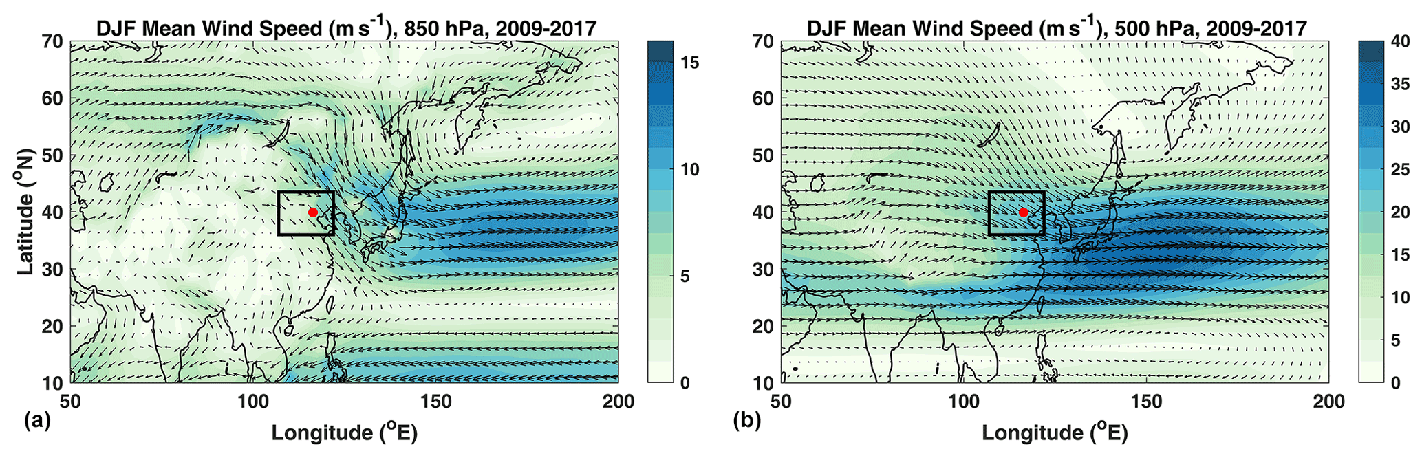
Figure 1 Average wind speeds at the (a) 850 hPa and (b) 500 hPa pressure levels. The red dot represents the location of Beijing and the black rectangle shows the location of the NCP. This figures was also generated for a longer average period, i.e. 1979–2019 (not shown), and the results were similar.

2 Data and methods

2.1 Observations, reanalysis outputs, and PPE model simulations

Hourly PM_2.5 concentrations from the US Embassy site for Beijing for DJF 2009–2017 are used. Daily mean PM_2.5 concentrations are constructed using hourly data to evaluate the performance of the HWI as a representative of haze-conducive and clear weather conditions for Beijing (see Sect. 3). We also use newly released gridded daily PM_2.5 concentrations for DJF from Chinese Air Quality Reanalysis (CAQRA) data provided by the China National Environment Monitoring Centre for 2013–2017 (Kong et al., 2021) to test the performance of the HWI across all of China. The CAQRA data were produced by assimilating surface air quality observations from over 1000 monitoring sites in China and are available at a high spatial resolution of around 15×15 km and hourly temporal resolution over China. More details on the validation of the CAQRA dataset against independent station data is provided in Kong et al. (2021). The visibility data for Beijing (homogenized data for 20 stations in Beijing) are provided by the National Meteorological Information Center of China, China Meteorological Administration (CMA), for DJF 1999–2018.

We use daily ERA-5 (fifth-generation ECMWF atmospheric reanalysis) data for four variables – meridional wind at the 850 hPa pressure level (V₈₅₀), zonal wind at the 500 hPa pressure level (U₅₀₀), and temperatures at the 850 hPa level (T₈₅₀) and the 250 hPa level (T₂₅₀) – to calculate the HWI for DJF 1979–2019. The ERA-5 data used here are available at 0.25^∘ × 0.25^∘ horizontal resolution and hourly temporal resolution (Hersbach et al., 2020).

We use a PPE of climate simulations produced using the recent configuration of the UK Met Office's HadGEM3-GC3.05 coupled model (Sexton et al., 2021; Yamazaki et al., 2021). The base model used for PPE, HadGEM3-GC3.05, has a horizontal resolution of ∼60 km with 85 vertical levels. A total of 47 model parameters from seven parameterization schemes were simultaneously perturbed to obtain the PPE (the full list of perturbed parameters is provided in Table 1 of Sexton et al., 2021). Here, we use daily outputs of V₈₅₀, U₅₀₀, T₈₅₀, and T₂₅₀ for DJF in the historical (1969–2005) and future (2006–2089) periods under the RCP8.5 scenario. In addition, we assess internal variability using 200-year control simulations for each PPE member where 1900 boundary conditions are prescribed. Overall, 16 PPE members are available for all the control, historical, and RCP8.5 simulations.

2.2 Calculation of the HWI

The winter HWI is calculated using the methodology given by Cai et al. (2017). We analyse the composite differences in U₅₀₀, V₈₅₀, T₈₅₀, and T₂₅₀ for hazy (PM_2.5 concentrations >150 µg m⁻³ for Beijing) and clear (PM_2.5 concentrations <35 µg m⁻³ for Beijing) days across China for DJF 2009–2017 (Fig. 2) (see Sect. 3.1 for an explanation of the PM_2.5 concentration cutoff values used here). We also provide the composite values for these meteorological variables for hazy and clear days separately in Fig. 2.

Figure 2 Winter composites of u-wind at the 500 hPa level (U₅₀₀) over China for all available days for which data were available from the US Embassy station for Beijing in DJF 2009–2017 for (a) high PM_2.5 (>150 µg m⁻³), (b) low PM_2.5 (<35 µg m⁻³) concentrations, and (c) the difference between the composites in (a) and (b). Panels (d–f) show the same as in (a–c) but for v-wind at the 850 hPa level (V₈₅₀); panels (g–i) show the same as in (a–c) but for temperature at the 850 hPa level (T₈₅₀), and panels (j–l) show the same as in (a–c) but for temperature at the 250 hPa pressure level (T₂₅₀). Black rectangles (B1–B5) in the last column show the regions for which spatial means were used for the calculation of the HWI. The blue dots in these panels show the location of Beijing.

During hazy days, the mid-tropospheric westerly flow becomes weaker over the NCP as compared to clear days (Fig. 2a–c). The mid-tropospheric trough also moves northwards, as suggested by the dipole pattern in Fig. 2c, which shows the differences in U₅₀₀ for hazy and clear days. The northerly flow in the lower troposphere is weaker during hazy days as compared to clear days (Fig. 2d–f). The lower troposphere is warmer during hazy days as compared to clear days (Fig. 2g–i), whereas the upper troposphere is cooler over the NCP (Fig. 2j–l). The changes in these variables are also consistent with previous studies (e.g. Cai et al., 2017) that showed similar changes for this time period. Therefore, we use these four variables for the calculation of the HWI, which is used as a proxy for haze-conducive and clear weather conditions under a future climate.

For the calculation of observational HWI, we use ERA-5 reanalysis data for the period 1979–2019. We first create a daily DJF time series of each variable for each reanalysis grid point over China. The daily DJF time series is concatenated for the period 1979–2019. A daily standardized anomaly time series is created for each meteorological variable by first removing the daily mean climatology from each day of the time series and then normalizing by the standard deviation. Spatial averages are then obtained over the relevant boxes (B1 to B5) for each meteorological variable following Cai et al. (2017) (Fig. 1). The HWI time series is calculated by using the following equation:

$$\begin{array}{}\text{(1)}& \text{HWI}\left(t\right)=U_{\mathrm{500}}\left(t\right)+V_{\mathrm{850}}\left(t\right)+\mathrm{d}T\left(t\right),\end{array}$$

where $U_{\mathrm{500}}=U_{\mathrm{500},\mathrm{B}\mathrm{1}}\left(t\right)-U_{\mathrm{500},\mathrm{B}\mathrm{2}}\left(t\right)$, $V_{\mathrm{850}}=V_{\mathrm{850},\mathrm{B}\mathrm{3}}\left(t\right)$, and $\mathrm{d}T=T_{\mathrm{850},\mathrm{B}\mathrm{4}}\left(t\right)-T_{\mathrm{250},\mathrm{B}\mathrm{5}}\left(t\right)$. The HWI(t) time series is then itself normalized by its own standard deviation.

For the PPE historical and RCP8.5 simulations, the daily HWI time series is calculated for each ensemble member for DJF for 1969–2089 using the same methodology as used for ERA-5, with the difference being that the normalization of the PPE time series (1969–2089) is performed using the historical standard deviation (1969–2005), following Cai et al. (2017). Similarly, the HWI time series is calculated for the PPE pre-industrial control simulations for 170 model years out of 200 model years (the first 30 years are discarded as the model spin-up period). The normalization of the pre-industrial control time series is performed using the standard deviation for 170 years. The pre-industrial control simulations used here are initialized with past forcings corresponding to the year 1900 and therefore are an approximate representation of the internal variability of the current climate, as this does not take into account any temporal changes in the internal variability from 1900 to the historical and future periods used here.

3 Haze weather index as an indicator for clear and haze-conducive weather conditions over the NCP

As the HWI was originally proposed for Beijing by Cai et al. (2017), we first determine if the HWI can be used as a representative of haze-conducive and clear weather conditions for the present climate for Beijing using (a) PM_2.5 concentrations from the US Embassy station in Beijing, (b) PM_2.5 concentrations averaged over a larger Beijing domain from CAQRA data, and (c) visibility data from the CMA stations in Beijing. We then determine the spatial extent of the region for which HWI can be used as an indicator of haze-conducive and clear weather conditions using PM_2.5 concentrations for China from CAQRA data. We use the 25th and 75th percentile values of daily mean PM_2.5 concentration to identify the clear and hazy days, respectively, for each dataset. For visibility, we use the opposite criterion, i.e. the 25th percentile as a threshold for hazy days and the 75th percentile as a threshold for clear days, as lower visibility is associated with hazy days and higher visibility with clear days. The days with a daily PM_2.5 concentration or visibility lying between the 25th and 75th percentile values are identified as moderately polluted days.

3.1 PM_2.5 concentrations for Beijing versus the HWI

We examine the relationship between the daily HWI and PM_2.5 concentrations for the US Embassy station for Beijing. Figure 3a shows that the daily HWI increases linearly with increasing PM_2.5 concentration for up to ∼150 µg m⁻³, and the HWI starts to level off when PM_2.5>150 µg m⁻³ (note the log scaling of the y axis). The time-series correlation between the HWI and PM_2.5 concentration is ∼0.58, which is significant at the 1 % level. Callahan et al. (2019) have also obtained a correlation coefficient of 0.58 for daily PM_2.5 concentrations from the US Embassy in Beijing and the HWI calculated using NCAR R1 reanalysis.

The 25th and 75th percentile values of daily mean PM_2.5 concentration for the US Embassy station in Beijing for DJF 2009–2017 are ∼35 and ∼150 µg m⁻³, respectively. We determine the percentage of hazy days (with daily mean PM_2.5 concentrations >150 µg m⁻³) and clear days (with daily mean PM_2.5 concentrations <35 µg m⁻³) for different HWI ranges (Fig. 3e). Out of all the days with HWI >1, 64 % have daily mean PM_2.5 concentrations of >150 µg m⁻³ and 98 % have PM_2.5 concentrations >35 µg m⁻³. This suggests that for HWI >1, almost all days are hazy or moderately polluted. Similarly, almost all days with HWI $>-\mathrm{1}$ are clear or moderately polluted. Using HWI thresholds of ±1 demarcates between the clear and hazy days, i.e. almost no clear days occur for HWI >1 and almost no hazy days occur for HWI $<-\mathrm{1}$.

We also examine the relationship between the individual variables in the HWI (Sect. 2.2) and PM_2.5 concentrations observed at the US embassy in Beijing/CAQRA and find that the individual components have correlation values that are similar to or less than the correlation values used in the combined HWI. Physically, multiple favourable weather conditions, as represented by each of these variables, collectively provide a conducive setting for haze. Hence, we focus on the HWI as a combined index rather than its individual components.

To examine if the PM_2.5 concentrations from the US embassy station are sensitive to the abrupt changes in the local meteorology, e.g. wind speeds or direction, we also examine the relationship between the HWI and PM_2.5 concentrations averaged over the domain centred around Beijing (116.15–116.65^∘ E, 39.65–40.15^∘ N) from the CAQRA data (Fig. 3b and f). The PM_2.5 concentrations for the region spatially averaged around Beijing from CAQRA data are in the range 6–441 µg m⁻³, and those from the Beijing US Embassy station are 6–569 µg m⁻³, suggesting that the values from both data sources are comparable. The correlation coefficient is ∼0.58, which is the same as the correlation obtained using the US Embassy data. The total numbers of hazy, clear, and moderately polluted days for different HWI ranges also show similar results for both datasets (Fig. 3e and f). This implies that the relationship of HWI with PM_2.5 concentration is robust across different data sources and that PM_2.5 is a regional pollutant.

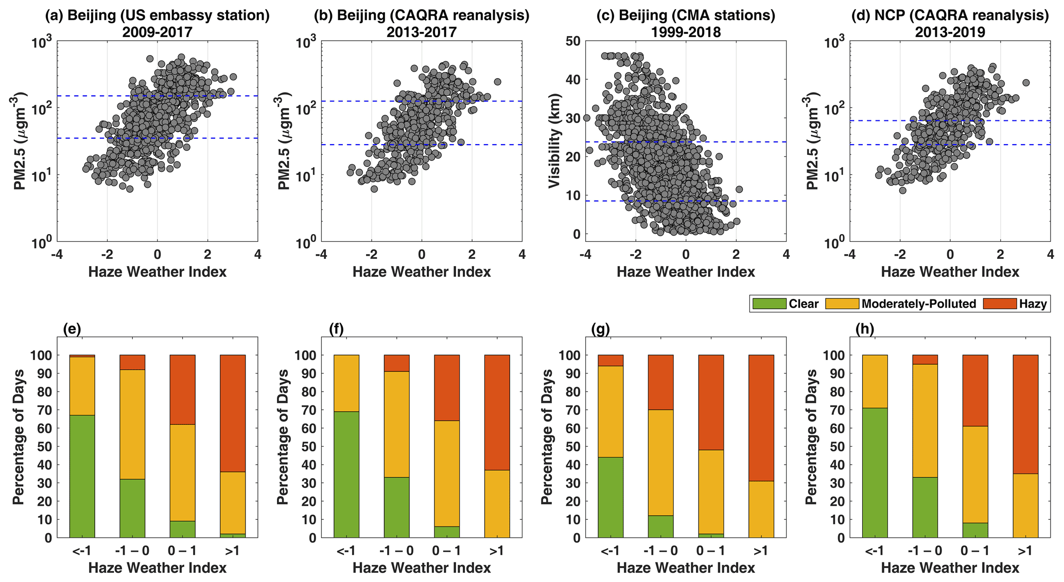
Figure 3 HWI versus daily mean (a) PM_2.5 concentration for the US Embassy station in Beijing for DJF 2009–2017, (b) PM_2.5 concentration spatially averaged over the region around Beijing (116.15–116.65^∘ E, 39.65–40.15^∘ N) from the CAQRA data for DJF 2013–2017, (c) visibility averaged over 20 stations from the CMA for DJF 1999–2018, and (d) PM_2.5 concentration spatially averaged over the NCP (36–43.5^∘ N, 107–122^∘ E) from the CAQRA data. Blue lines show the 25th and 75th percentile thresholds used to define clear and hazy days for each dataset. Percentages of clear, moderately polluted, and hazy days for different HWI ranges for (e) the US Embassy station in Beijing for DJF 1999–2018, (f) a larger Beijing domain (116.15–116.65^∘ E, 39.65–40.15^∘ N) from the CAQRA data for DJF 2013–2017, (g) Beijing for DJF 1999–2018, and (h) the NCP from the CAQRA data for DJF 2013–2017.

3.2 Visibility for Beijing versus the HWI

As visibility is an optical representative of haze (Wang et al., 2006) and visibility data are available for a relatively long period (1999–2018) as compared to PM_2.5 concentration data, we also correlate the HWI with the visibility over Beijing. Figure 3c shows that the HWI is inversely related to the visibility for the Beijing station. The time-series correlation between the HWI and visibility is −0.63, which is significant at the 1 % level. The days with visibility <8.5 km are identified as hazy days, while days with visibility >23.8 km are identified as clear days. For days with HWI >1, no clear days occur; similarly, for days with HWI $<-\mathrm{1}$, only 6 % of the days are hazy (Fig. 3g). This further confirms that the correlation between the HWI and haze is significant for a longer period (1999–2018) when using visibility as a metric for haze (as an alternative to the PM_2.5 concentrations used above).

3.3 PM_2.5 concentrations over the North China Plain versus the HWI

We now determine the spatial extent for which HWI can be used as an indicator of haze-clear or haze-conducive conditions using PM_2.5 concentrations from CAQRA data. We correlate the daily time series of PM_2.5 concentration at each grid point with the HWI for DJF 2013–2017 (Fig. 4). Over the entire NCP (36–43.5^∘ N, 107–122^∘ E), the correlation coefficient between the daily HWI and gridded PM_2.5 concentration is ∼0.7, which is significant at the 1 % level. The correlation is considerably lower but still significant over other eastern China regions, e.g. north easternmost China and the Sichuan Basin (27–32^∘ N, 102–107^∘ E).

Figure 4 Spatial distribution of the correlation between winter PM_2.5 concentration and HWI time series at each grid point. Blue dot shows the Beijing station (39.3^∘ N, 116.4^∘ E) and the black rectangle shows the North China Plain (36–43.5^∘ N, 107–122^∘ E).

Considering daily mean PM_2.5 concentrations averaged over the NCP, we also find a linear relationship with the daily HWI (r=0.66, significant at the 1 % level; Fig. 2d). We also calculate the percentages of clear and hazy days for different HWI ranges for the larger domain of the NCP using the 25th and 75th percentile values, respectively. The percentages of hazy and clear days for HWI >1 and HWI $<-\mathrm{1}$ for the NCP in CAQRA data are very similar to the values obtained for the US Embassy station in Beijing (Fig. 3h).

Overall, our results confirm that the daily HWI has a robust relationship with daily PM_2.5 concentrations not only for the Beijing station but across the NCP for the given time periods. Therefore, we use HWI >1 as a proxy for haze-conducive weather and HWI $<-\mathrm{1}$ as a proxy for clear weather across the NCP region. This threshold is also consistent with several other studies (e.g. Cai et al., 2017; Callahan and Mankin, 2020; Callahan et al., 2019) that have used HWI >1 as a cutoff for haze-conducive weather for Beijing. We now calculate the frequencies of haze-conducive weather (HWI >1) and clear weather (HWI $<-\mathrm{1}$) for the past and future using the ERA-5 reanalysis and PPE members.

4 Historical and future changes in haze-conducive and clear weather occurrence

The frequencies of haze-conducive weather (HWI >1) and clear weather (HWI $<-\mathrm{1}$) from the ERA-5 data and the PPE are shown in Fig. 5. For ERA-5, the frequency of haze-conducive weather has increased whereas the frequency of clear weather (HWI $<-\mathrm{1}$) has reduced for the period 1979–2018. The mean frequency of haze-conducive weather using 16 PPE members shows a larger increase than ERA-5 for the same 1979–2018 time period (Fig. 5a). In contrast, the mean frequency of clear weather from the PPE for this period shows a similar reduction to that obtained using the ERA-5 reanalyses (Fig. 5b).

We examine the changes in the frequencies of haze-conducive weather (HWI >1) and clear weather (HWI $<-\mathrm{1}$) for the historical period (1979–2005) and three future periods, i.e. the near (2006–2032), mid- (2033–2059), and far (2060–2086) future. The mean frequency of haze-conducive weather is 14.7 d per winter from the ERA-5 data and 15.0 d per winter from the PPE mean for the historical period. The corresponding values for clear weather are 15.0 and 15.2 d per winter for ERA-5 and PPE, respectively. This shows that there is good agreement between the mean frequencies of haze-conducive and clear weather for the ERA-5 data and the PPE mean for the historical period.

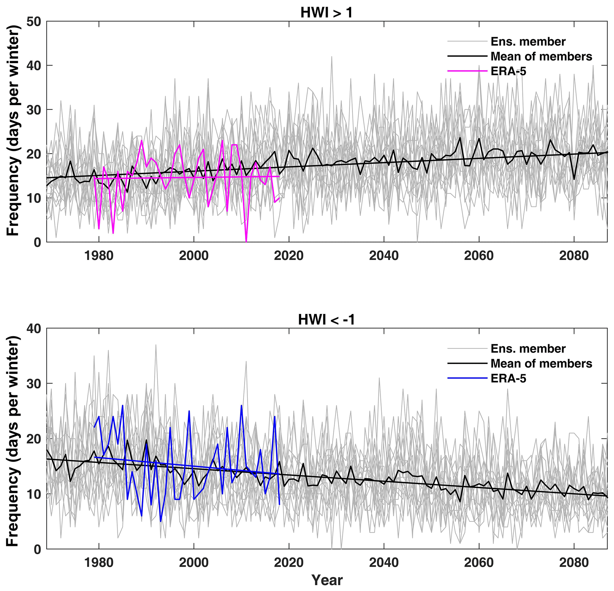
Figure 5 Frequencies of haze-conducive weather (HWI >1, pink line) and clear weather (HWI $<-\mathrm{1}$, blue line) per winter from ERA-5 reanalysis (1979 to 2018). The year 1979 represents the period from 1 December 1979 to 28 February 1980, and so on. For each winter (DJF), we calculate the total number of days with HWI >1 as a proxy for haze-conducive weather and HWI $<-\mathrm{1}$ as a proxy for clear weather conditions. Grey lines show frequencies from 16 individual PPE members and the black line shows the mean frequency calculated using all 16 PPE members for 1969–2087 under the RCP8.5 scenario. The linear trend is calculated using the line of best fit.

The mean frequency of haze-conducive weather in the near, mid-, and far future is 17.9, 18.6, and 19.9 days per winter, respectively. The mean frequency of clear weather in the same future periods is 13.2, 12.2, and 10.8, respectively (Fig. 6a). The mean change in the frequency of haze-conducive weather averaged across all PPE members is 20 %, 24 %, and 33 % for the near, mid-, and far future, respectively, as compared to the historical period, suggesting that the frequency of haze-conducive weather will likely increase in all future periods (Fig. 6a). However, the projected change has a very large range in all three future periods, suggesting that internal variability or the parametric effect could influence future projections of haze-conducive weather. For the near and mid-future, the number of days with HWI >1 is projected to change by −1 % to 41 % and by −12 % to 65 % across the 16 PPE members, respectively, as compared to the frequency in the historical period. For the far future, the range of projected change is even larger, and an increase of ∼87 % in the frequency of haze-conducive weather is also possible. It is noted that, for all three periods, only one of the 16 ensemble members (E16, shown in Fig. 10) shows a reduction in haze-conducive weather frequency, whereas the other ensemble members show an increase in frequency in all periods. For the historical period, ensemble member E16 presents a mean frequency of 16.3, which reduces to 16.2, 14.4, and 15.2 in the near, mid-, and far future. While ensemble member E16 shows a consistent reduction in mean frequency in the future, the reduction is specific to this ensemble member only; it is not a general feature for PPE members.

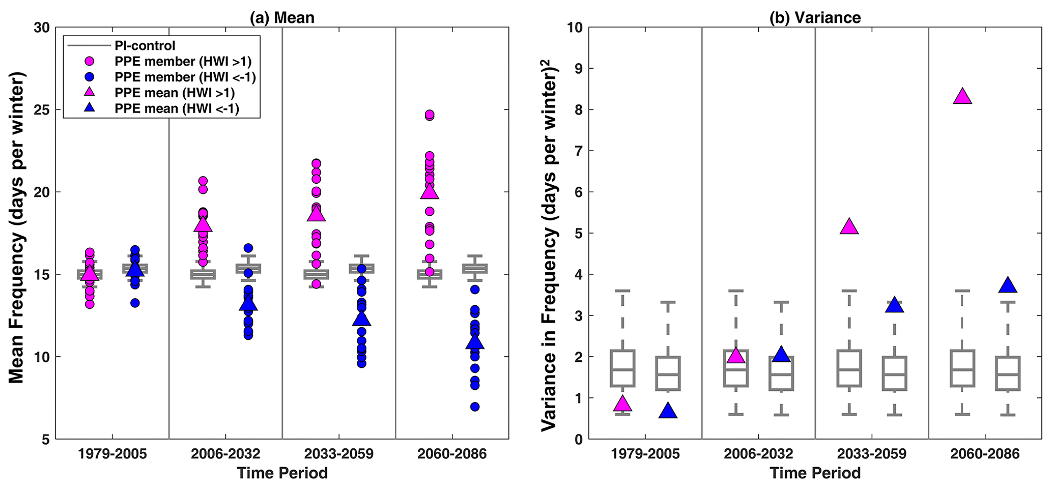
Figure 6 (a) Mean frequencies of haze-conducive weather (HWI >1, pink) and clear weather (HWI $<-\mathrm{1}$, blue) for the historical period (1979–2005) and for the near (2006–2032), mid- (2033–2059), and far (2060–2086) future under the RCP8.5 scenario. Circles represent PPE members and triangles show the PPE mean. Grey boxes and whiskers show the distributions of 10 000 mean frequency values sub-sampled from the control simulation. Panel (b) is the same as (a) but it shows the variance across the 16 PPE members for each period. For each box and whiskers, we first randomly sampled 10 000 time series, each of length 27 years, using 2704 years of pre-industrial control simulation and calculated 10 000 values of mean frequency. We then randomly sub-sampled 16 mean values (corresponding to the number of ensemble members) from the 10 000 mean values and calculated their mean (a) and variance (b). This was repeated 10 000 times to obtain a distribution. The boxes are at the 25th and 75th percentiles and the whiskers are at the 2.5th and 97.5th percentiles of the mean and variance distributions. For panel (a), the box and whiskers are comparable only for the ensemble means (triangles) and not the ensemble members (circles).

For clear weather (HWI $<-\mathrm{1}$), the mean change in the frequency averaged across all PPE members is −13 %, −20 %, and −29 % for the near, mid-, and far future, respectively (Fig. 6a). Considering the range across the 16 PPE members, the frequency of clear weather in the near, mid-, and far future is projected to change by −29 % to 25 %, −36 % to 10 %, and −57 % to −9 %, respectively. Overall, most ensemble members show an increase in the frequency of haze-conducive weather and a reduction in the frequency of clear weather for all three future periods. However, a negligible change or even the opposite change is possible, though less likely, for all periods.

We also determine the influences of anthropogenic climate change and the parametric effect on the frequencies of haze-conducive weather (HWI >1) and clear weather (HWI $<-\mathrm{1}$) for the historical as well as the three future periods. As shown later (Sect. 5), the estimate of the interannual variance from the control is representative of all time periods and shows no discernible parametric effect. Therefore, we pool the 16 PPE control simulations to sample the internal variability for the boxes and whiskers shown in Fig. 6a and b (see captions for details on resampling).

In Fig. 6a, we show the mean frequencies of haze-conducive weather and clear weather for the 16 individual PPE members (circles) and the PPE mean (triangles). Each grey box and whiskers represents the range of ensemble mean frequencies that can be explained by the internal variability. If the PPE mean (triangles) lies within the whiskers (i.e. the 95th percentile of the control distribution), we can conclude that there is no influence of anthropogenic climate change on the mean frequency; however, if the PPE mean lies outside the whiskers, it would represent a climate change signal in the mean frequency. Figure 6a suggests that the mean frequencies of haze-conducive as well as clear weather lie within the box and whiskers for the historical period but outside the whiskers for the three future periods, thereby showing a clear impact of anthropogenic climate change on the frequencies of both haze-conducive and clear weather conditions.

We now examine whether the differences in mean frequency across PPE members (shown by circles in Fig. 6a) for a given period can be explained by the internal variability or if the differences between PPE members partly arise due to the parametric effect. The triangles in Fig. 6b show the variance across the 16 PPE members, i.e. the variance across the 16 circles shown in Fig. 6a, for each time period. The whiskers in Fig. 6b show the 95 % confidence interval from the control simulation, which is representative of the internal variability. For any time period, if the PPE member variance (triangle) lies within the whiskers, we can conclude that the differences in mean frequencies in Fig. 6a can be fully explained by the internal variability, and there is no discernible impact of the parametric effect. However, if the triangles lie outside the whiskers in Fig. 6b, we can conclude that there is an impact of the parametric effect on the mean frequency for that period. For the points that lie outside the whiskers in Fig. 6b, we also quantify the percentages of the variance that can be explained by the internal variability and the parametric effect. For any time period, the variance in the ensemble mean due to the parametric effect is simply calculated as follows (the remaining variance is attributed to the internal variability):

$$\begin{array}{}\text{(2)}& \begin{array}{rl}& {\displaystyle \frac{\text{Total variance in the ensemble mean}-\text{Mean variance from the control simulation}}{\text{Total variance in the ensemble mean}}}\\ & \times \mathrm{100}.\end{array}\end{array}$$

Figure 6b shows that the differences in mean frequency across PPE members (as shown by the PPE member variance) are small for the historical and near future but increase for the mid- and far-future periods. For the historical and near-future periods, the PPE member variance lies within the range sampled by the internal variability for both haze-conducive weather (HWI >1) and clear weather (HWI $<-\mathrm{1}$). This shows that there is no discernible influence of the parametric effect on the frequency of haze-conducive weather or clear weather conditions for the historical and near-future periods.

For the mid-future, the PPE member variance for clear weather lies within the whiskers and therefore no discernible influence of the parametric effect is detected. In contrast, the PPE member variance for haze-conducive weather lies outside the whiskers and the internal variability can explain ∼33 % of the variance across PPE members; the remaining ∼67 % arises due to the parametric effect.

For the far future, triangles corresponding to both haze-conducive and clear weather lie well outside the whiskers and therefore show a clear influence of the parametric effect. Only ∼20 % of the variance in the frequency of haze-conducive weather and ∼43 % of the variance in the frequency of clear weather can be explained by the internal variability, with the remaining 80 % and 57 % of the respective frequency variances arising due to the parametric effect.

Figure 7 Frequency of haze-conducive weather (HWI >1) versus frequency of clear weather (HWI $<-\mathrm{1}$) averaged over the historical period (1979–2005) and the far-future (2060–2086) period under RCP8.5 using all PPE members. Small coloured circles denote individual PPE members whereas large coloured circles denote the means of the members. The grey circle shows the mean frequency from ERA-5 reanalysis for the historical period (1979–2005). The black solid line shows the 1:1 (identity) line.

In addition to the changes in the frequencies over time, we also investigate the relative changes in the frequency of haze-conducive weather (HWI >1) versus the frequency of clear weather (HWI $<-\mathrm{1}$). The average haze-conducive and clear weather frequencies over the historical period are almost equal for each PPE member (Fig. 7). All PPE members show a higher frequency of haze-conducive weather than of clear weather in the far future (2060–2085); however, there is a substantial range of change. The frequency of winter-haze-conducive weather can be similar to or up to 3.5 times the frequency of clear weather conditions (Fig. 7). Similar results are also obtained for the near and mid-future. Averaged across the PPE members, the number of haze-conducive days can increase by ∼2 times as compared to the number of clear days in the future. As noted in Fig. 7, the spread in the haze-conducive weather frequency amongst individual ensemble members is also larger for the far future (2060–2086) compared to the historical period. This suggests a larger uncertainty and a larger range of possible future meteorological conditions affecting haze and air quality as compared to the historical period. Other studies (e.g. Cai et al., 2017; Callahan and Mankin, 2020) have also found similar increases in the frequency of haze-conducive weather for the future. However, the range of projected change differs substantially between models as well as ensemble members. In our study, in addition to the frequency of haze-conducive weather, we also evaluate the changes in the frequency of clear weather in different future periods and compare the relative changes in both frequencies, which were not examined in past studies.

We now investigate changes in the distribution of the HWI as well as individual constituents of the HWI in the far future (2060–2086) as compared to the historical (1979–2005) period. The probability distribution of the HWI shows a shift towards higher magnitudes for the far future as compared to the historical period (Fig. 8). This implies an increased frequency of haze-conducive weather, as the number of days with HWI >1 increases. Similar shifts are apparent in the zonal-mean wind (U₅₀₀) and vertical temperature (dT) profiles, whereas no apparent shift is noted in V₈₅₀. We also find that the shift in the HWI as well those in as the U₅₀₀ and dT distributions are not due to the shift in one particular PPE member or time period: they are consistent across the 16 PPE members and are continual over time from the historical to the far-future period. Therefore, for the PPE analysed here, the changes in the haze-conducive weather (HWI >1) are largely associated with the changes in U₅₀₀ and dT, and V₈₅₀ appears to have a less important role. Despite using a multimodel ensemble and a different time period than used here, a similar result but with larger shifts in the PDFs of U₅₀₀ and dT as compared to V₈₅₀ is also noted in Cai et al. (2017).

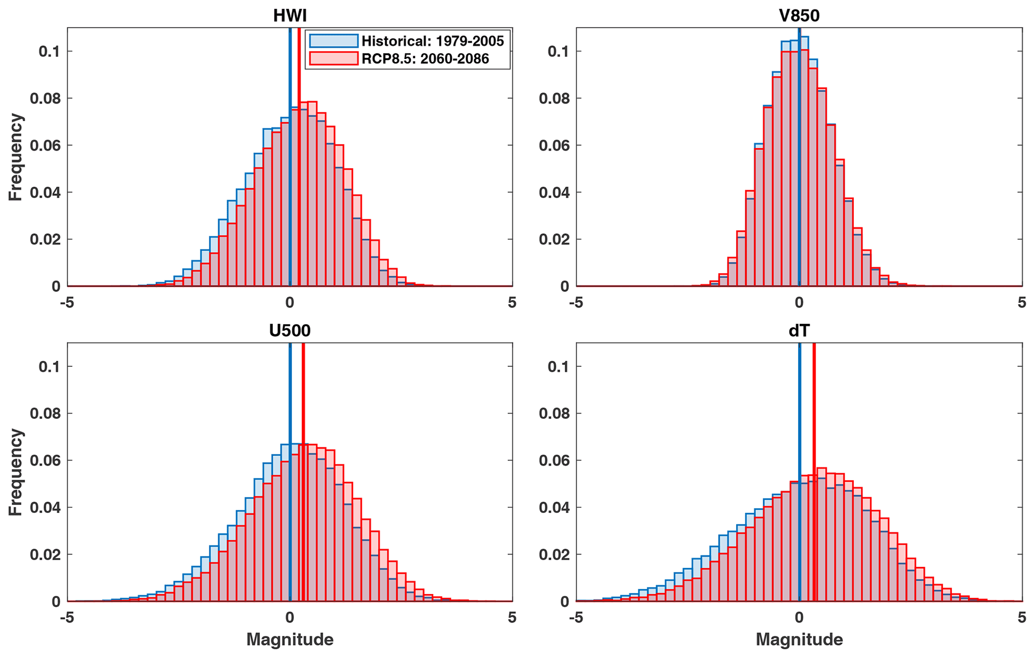
Figure 8 Probability distribution functions (PDFs) for the winter HWI, meridional winds at the 850 hPa pressure level (V₈₅₀), zonal winds at the 500 hPa pressure level (U₅₀₀), and temperature gradient between the lower and upper troposphere (dT). The PDF for the HWI was created using the daily DJF time series of all 16 PPE members. The PDFs for V₈₅₀, U₅₀₀, and dT were created using the normalized daily DJF time series of each variable calculated for the HWI (see Sect. 2.2 for details) and represent the constituent variables of the HWI. Blue bars show the PDFs for the historical period and red bars show the PDFs for the far future under the RCP 8.5 scenario. Solid blue and solid red lines show the mean values of the PDF for the historical and far-future periods, respectively.

5 Interannual variability in haze-conducive and clear weather frequency

Large interannual variability in the frequencies of haze-conducive (HWI >1) and clear weather (HWI $<-\mathrm{1}$) is apparent in both individual PPE members and the ERA-5 reanalysis (Sect. 4). Therefore, we examine the changes in the interannual variances of these frequencies for future periods as compared to the historical period. We also compare the variances in historical and future time periods with the variance in the control simulation to discern the influence of the model physical parameterizations, i.e. the parametric effect, on the variance.

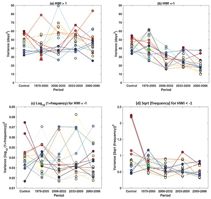
Figure 9 Interannual variances in the frequencies of winter (a) haze-conducive weather (HWI >1) and (b) clear weather (HWI $<-\mathrm{1}$) for the control simulation and the historical (1979–2005), near-future (2006–2032), mid-future (2033–2059), and far-future (2060–2086) periods under RCP8.5 for all 16 PPE members. Coloured circles are plotted for individual PPE members and triangles for the ERA-5 data. Panels (c, d) are same as (b) but with log₁₀ and square-root power transformations. For (c) and (d), we first calculated the log₁₀ of (1 + frequency) and the square root of the frequency of clear days for the control simulation and each time period, and then we estimated the variance for each respective period. The lengths of the control simulation and all future periods are the same as that of the historical period, i.e. 27 years. The 27 years used for the control here were randomly selected from a 170-year control simulation for each member.

The interannual variance for the ERA-5 data is 27 and 39 d² for haze-conducive and clear weather, respectively, for the historical period (1979–2005) (triangles in Fig. 9a and b). The interannual variance in haze-conducive weather frequency derived from the PPE members for the historical period is larger than that for ERA-5, whereas for the clear weather, the variance for ERA-5 lies within the range of the PPE members. No consistent change in the interannual variance of haze-conducive weather is noted for any of the PPE members (note the changes in colour ranking) from the historical to the future periods, suggesting little influence of the parametric effect on the interannual variance of haze-conducive weather.

In contrast, the frequency of clear weather for most PPE members shows a marked reduction in interannual variance from the historical to the near-future period (Fig. 9b). However, as the frequency of clear weather shows a decreasing trend over time (see Fig. 5b), the mean frequency would be expected to reduce for the three future periods. Also, the reduction in variance could arise as the frequencies of clear weather approach their lower bound of zero. With count data, a power transformation is often applied to stabilize the variance across all time periods. We applied two power transformations, i.e. log₁₀(1 +x) and square root (x), where x is the count data (Fig. 9c and d). We find that the spread in the variance in the control simulation across the PPE members is comparable with those in the historical as well as future periods (Fig. 9c and d). Note that for the control simulation, we randomly selected 27 years (the same length as for the historical and future periods) from 170 years of control simulation for each PPE member; however, we note comparable variance for the other randomly selected samples. Figure 9c and d also show that the individual PPE members show inconsistent changes in the variance (noting changes in the colour ranking) from control to historical and future periods. Therefore, no robust changes can be detected in the interannual variances of haze-conducive and clear weather from control to historical and future periods. This means that we can use the variance in the control simulation as a representative estimate of internal variability. This enables us to quantify the influences of the parametric effect and anthropogenic climate change on the mean frequencies (see the previous section) and trends in frequencies (see the next section) across different periods.

6 Influences of anthropogenic climate change and the parametric effect on trends

We discern the influences of anthropogenic climate change and the parametric effect on future projections of the trends in the frequency of haze-conducive weather (HWI >1) and the frequency of clear weather (HWI $<-\mathrm{1}$). The time series of the haze-conducive and clear weather frequencies from ERA-5 and the 16 PPE members for the historical and future periods are shown in Fig. 10a and b. The 95th percentile values (blue-shaded regions) and the ranges (dotted blue lines) of the haze-conducive and clear weather frequencies from the respective control simulation for each PPE member are also shown.

For haze-conducive weather (HWI >1), the time series for selected PPE members (e.g. E3, E4) show increasingly positive trends. In particular, towards the end of the 21st century (Fig. 10a), the lower half of the control range is seldom sampled, and more than the expected number of values lie above the 97.5th percentile of the control frequencies. In contrast, for other PPE members (e.g. E8, E10), the full time series samples the control distribution evenly throughout the full period. For clear weather (HWI $<-\mathrm{1}$), some members (e.g. E3, E4) show a clear reduction during the 21st century whilst others (e.g. E16) show no trend and explore the control distribution evenly (Fig. 10b).

In Sect. 4, we examined the influences of anthropogenic climate change and the parametric effect on the mean frequencies. The analysis of mean frequencies provides an estimate of the accumulated influence of climate change on the frequencies with respect to the control simulations, whereas analysis of trends provides a better estimate of changes within a selected time period. Therefore, we apply the same analysis on the trends in the frequencies (Fig. 11).

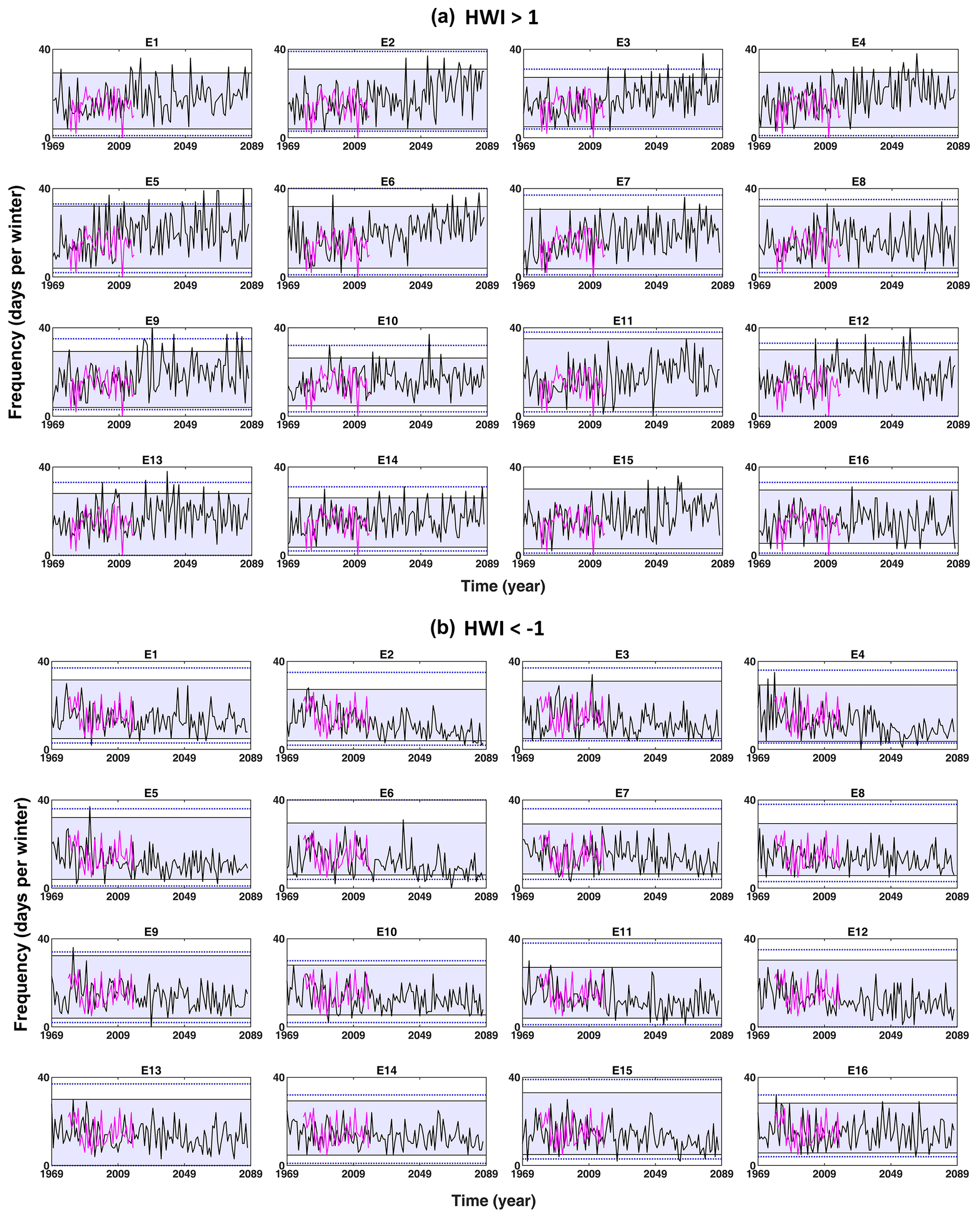
Figure 10 Frequency of (a) haze-conducive weather (HWI >1) and (b) clear weather (HWI $<-\mathrm{1}$) per winter for individual PPE members (black line) under the historical and RCP8.5 scenarios for 1969–2087 and the ERA-5 reanalysis (pink line) for 1979–2018. The blue-shaded regions show the 95th confidence intervals and the dotted blue lines shows the ranges of haze-conducive and clear weather frequency for the pre-industrial control simulation of 170 years.

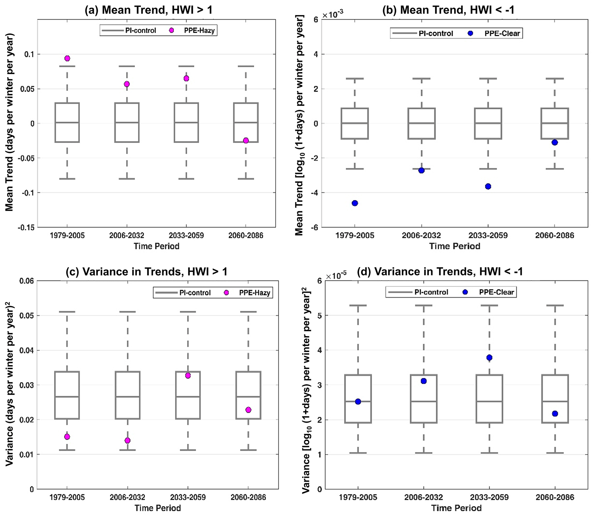
Figure 11 Mean PPE trends for the frequencies of (a) haze-conducive weather (HWI >1) and (b) clear weather (HWI $<-\mathrm{1}$) in winter. Circles show the mean trends from 16 PPE members for the historical (1979–2005) and the near-future (2006–2032), mid-future (2033–2059), and far-future (2060–2086) periods under the RCP8.5 scenario. Each grey box and whiskers shows the distribution of 10 000 values of trends sub-sampled from the control simulation. Panels (c, d) show the same as in (a, b) but the mean is replaced by the variance in trends. For each box and whiskers, we first randomly sampled 10 000 time series of length 27 years using 2704 years of pre-industrial control simulation and calculated 10 000 values of trends. We then randomly sub-sampled 16 trend values from the 10 000 trend values and calculated the variance and mean of those 16 trend values. The boxes are at the 25th and 75th percentiles and the whiskers are at the 2.5th and 97.5th percentiles of the mean and variance distributions. For clear days, the frequencies were transformed to log space by applying a power transformation of log₁₀(1 + frequency) before calculating trends.

We calculate the ensemble mean trend obtained from the 16 individual PPE member trends to determine the influence of climate change for the historical period (see captions of Fig. 11 for details). We describe the evolution of the historical trend for three equal-length future time periods (i.e. the near, mid-, and far future) and we examine whether the historical trends are sustained across the 21st century and if the trends are discernible outside the range described by the internal variability (Fig. 11a and b). The grey whiskers in Fig. 11a and b cover the range of trends that can be explained by internal variability, and any trend values lying outside the grey whiskers represent the influence of anthropogenic climate change.

The mean trends in the frequencies of both haze-conducive weather (HWI >1) and clear weather (HWI $<-\mathrm{1}$) for the historical period (1979–2005) lie outside the 95 % confidence interval of the control simulations. This suggests that the trends noted for the historical period cannot be explained by internal variability alone and there is a substantial impact of anthropogenic climate change on the historical trends. The trends in haze-conducive weather lie within the envelope of internal variability for the three future periods analysed here, implying that the historical trend is not sustained over the 21st century and is indistinguishable from the internal variability for the future. Figure 11a also shows a positive mean trend in haze-conducive weather (HWI >1) for the historical, near-future, and mid-future periods, but a weak negative trend for the far future. While the frequency of haze-conducive weather increases for all three future periods with respect to the historical period, as shown in Fig. 6a, the trends only show an increment or reduction for that period, as these are not referenced to the historical period. Therefore, trends can still be negative within any selected period, as in the case of the far future. In contrast, the mean trends in clear weather frequency for the near future (2006–2032) and the mid-future (2033–2059) lie outside the 95 % confidence interval of the control simulation. This shows that for clear weather frequency (HWI $<-\mathrm{1}$), the historical trend is sustained over the first half of the 21st century and then it levels off.

We now examine the influence of the parametric effect on the trends in the frequencies of haze-conducive and clear weather. In Fig. 11c and d, we show the variance in trends for the time series resampled using the control simulation (see the captions for details on resampling). The grey box and whiskers shows the 95 % confidence interval of the control variance used to represent the internal variability. The variance in the PPE trends calculated using the 16 PPE members for each selected time period is overlaid (circle). In Fig. 11c and d, if the variance for the historical or a future period lies outside the whiskers, we conclude that the parametric effect has an impact on the trends. However, if the variance across the 16 PPE members lies within the whiskers, we conclude that there is no impact of the parametric effect on the trend. Note that the variance in the trends for clear weather is in log-transformed space. As can be seen in Fig. 11c and d, the variance in PPE trends for the historical and future periods lies within the 95th percentile distribution of the internal variability for both haze-conducive and clear weather. Therefore, we do not find any discernible influence of the parametric effect on the trends in the frequencies.

7 Conclusions

In this study, we elucidated, for the first time, the influence of model physical parametrizations, in addition to those of internal variability and climate change, on the future haze-conducive and clear weather conditions over the North China Plain (NCP) using the perturbed parameter ensemble (PPE) from the Met Office's HadGEM3-GC3.05 model. We examined the changes in winter (December–February) haze-conducive and clear weather conditions in the past and future over the NCP using a large-scale meteorology-based daily haze weather index (HWI). We first identified the regional extent of the application of the HWI over China. We found that the HWI >1 can be used as an indicator of haze-conducive weather conditions and HWI $<-\mathrm{1}$ as an indicator of clear weather conditions for the entire NCP due to the spatial coherence of regional meteorological conditions over this region.

The PPE shows that under the RCP8.5 emission scenario, the mean frequency of haze-conducive weather (HWI >1) can increase by up to ∼65 % in the near (2006–2032) and mid- (2033–2059) future and by ∼87 % in the far future (2060–2086) as compared to the historical period (1979–2005). In contrast, the frequency of clear weather (HWI $<-\mathrm{1}$) can reduce by up to ∼40 % in the near and mid-future and by ∼57 % in the far future. Nevertheless, a reduction in the frequency of haze-conducive weather and increment in the frequency of clear weather, though less likely, is also possible. The absolute number of days with haze-conducive weather in the far future can remain the same or increase by up to ∼3.5 times of the number of days of clear weather over the NCP. There is also large interannual variability in the frequencies of haze-conducive and clear weather conditions. However, no systematic change in the interannual variance of the frequency is noted for the future as compared to the historical period. We also find that enhanced vertical thermal stability due to the warming of the troposphere and weaker northwesterlies over the NCP in the mid-troposphere will collectively lead to more frequent haze-conducive weather over the NCP. We find a consistently growing influence of anthropogenic climate change and the parametric effect on the mean haze-conducive and clear weather frequencies across the 21st century. This suggests that, in addition to the internal variability, the parametric effect adds an additional source of uncertainty to future projections of haze-conducive and clear weather, particularly towards the end of the 21st century. We find that the impact of anthropogenic climate change is discernible in trends for the historical period for haze-conducive weather and up to the middle of the 21st century for clear weather. Beyond those periods, the historical trends are not sustained and not distinguishable from the internal variability.

This study considered four atmospheric variables to examine the changes in future haze-conducive and clear weather conditions; however, other atmospheric variables (e.g. boundary layer height) or processes may influence the occurrence of haze. Furthermore, even though our study shows the potential for an increase in haze-conducive weather conditions and a reduction in clear weather conditions for the future periods, the actual formation of haze will depend on future emissions of air pollutants and their precursors. If the source emissions are cut off or reduced in the future, the risk of haze formation will naturally reduce. Nevertheless, projections of changes in the frequency and interannual variance of haze-conducive weather conditions can be very useful for developing successful adaptation and mitigation policies for the future that consider both emissions and climate change, and can therefore be beneficial for near- and long-term planning and decision making in relation to improving future PM_2.5 air quality.