the Creative Commons Attribution 4.0 License.
the Creative Commons Attribution 4.0 License.
 | 09 Jun 2022
Australian wildfire smoke in the stratosphere: the decay phase in 2020/2021 and impact on ozone depletion
Albert Ansmann
Bernd Kaifler
Alexandra Chudnovsky
Boris Barja
Daniel A. Knopf
Natalie Kaifler
Holger Baars
Patric Seifert
Diego Villanueva
Cristofer Jimenez
Martin Radenz
Ronny Engelmann
Igor Veselovskii
Félix Zamorano
Record-breaking wildfires raged in southeastern Australia in late December 2019 and early January 2020. Rather strong pyrocumulonimbus (pyroCb) convection developed over the fire areas and lofted enormous amounts of biomass burning smoke into the tropopause region and caused the strongest wildfire-related stratospheric aerosol perturbation ever observed around the globe. We discuss the geometrical, optical, and microphysical properties of the stratospheric smoke layers and the decay of this major stratospheric perturbation. A multiwavelength polarization Raman lidar at Punta Arenas (53.2∘ S, 70.9∘ W), southern Chile, and an elastic backscatter Raman lidar at Río Grande (53.8∘ S, 67.7∘ W) in southern Argentina, were operated to monitor the major record-breaking event until the end of 2021. These lidar measurements can be regarded as representative for mid to high latitudes in the Southern Hemisphere. A unique dynamical feature, an anticyclonic, smoke-filled vortex with 1000 km horizontal width and 5 km vertical extent, which ascended by about 500 m d−1, was observed over the full last week of January 2020. The key results of the long-term study are as follows. The smoke layers extended, on average, from 9 to 24 km in height. The smoke partly ascended to more than 30 km height as a result of self-lofting processes. Clear signs of a smoke impact on the record-breaking ozone hole over Antarctica in September–November 2020 were found. A slow decay of the stratospheric perturbation detected by means of the 532 nm aerosol optical thickness (AOT) yielded an e-folding decay time of 19–20 months. The maximum smoke AOT was around 1.0 over Punta Arenas in January 2020 and thus 2 to 3 orders of magnitude above the stratospheric aerosol background of 0.005. After 2 months with strongly varying smoke conditions, the 532 nm AOT decreased to 0.03-0.06 from March–December 2020 and to 0.015–0.03 throughout 2021. The particle extinction coefficients at 532 nm were in the range of 10–75 Mm−1 in January 2020 and, later on, mostly between 1 and 5 Mm−1. Combined lidar–photometer retrievals revealed typical smoke extinction-to-backscatter ratios of 69 ± 19 sr (at 355 nm), 91 ± 17 sr (at 532 nm), and 120 ± 22 sr (at 1064 nm). An ozone reduction of 20 %–25 % in the 15–22 km height range was observed over Antarctica and New Zealand ozonesonde stations in the smoke-polluted air, with particle surface area concentrations of 1–5 µm2 cm−3.
- Article
(15018 KB) - Full-text XML
- BibTeX
- EndNote


Extremely strong and long-lasting bushfires in southeastern Australia (Boer et al., 2020), in combination with extraordinarily strong pyrocumulonimbus (pyroCb) activity at the end of December 2019 and at the beginning of January 2020, induced a major perturbation of the stratospheric aerosol conditions (Peterson et al., 2021). The smoke dispersed over most parts of the Southern Hemisphere, including Antarctica (Tencé et al., 2021), and reached heights up to 35 km (Khaykin et al., 2020; Kablick et al., 2020). The Black Summer fire season of 2019–2020 in southeastern Australia, denoted as Australian New Year Super Outbreak (ANYSO) event by Peterson et al. (2021), caused a 3 times higher stratospheric aerosol mass of injected smoke than the record-breaking Canadian wildfires (Pacific Northwest Event, PNE) in the Northern Hemisphere in August 2017 (Peterson et al., 2018). The latter led to the largest stratospheric perturbation by smoke over Germany (Ansmann et al., 2018) and Europe (Baars et al., 2019). The ANYSO-related maximum monthly mean aerosol optical thickness (AOT) for the latitudinal belt from 20 to 70∘ S exceeded even the maximum AOT (for these southern latitudes) in this latitudinal belt observed after the major eruption of the Pinatubo volcano (Hirsch and Koren, 2021). The stratospheric smoke particles influenced climate conditions (Hirsch and Koren, 2021; Heinold et al., 2021; Stocker et al., 2021) and probably also led to the record-breaking ozone depletion in Antarctica in September 2020 (Stone et al., 2021).
Wildfire smoke particles, mainly consisting of brown carbon with a few percent of black carbon (Hems et al., 2021), considerably absorb solar radiation and can perturb shortwave and longwave radiative fluxes and thus dynamical processes. Several Australian smoke plumes were found to significantly alter the dynamic circulation in the lower stratosphere (Khaykin et al., 2020; Kablick et al., 2020; Allen et al., 2020; Lestrelin et al., 2021). The potential of smoke to ascend over several months by heating the air due to strong light absorption is an important aspect that significantly prolongs the residence time of wildfire smoke in the stratosphere. As Peterson et al. (2021) pointed out, the diabatic lofting effect is often strong enough to oppose the mean downward motion, ultimately increasing plume lifetime in the stratosphere. Several ANYSO smoke events ascended from initial injection heights of 14–17 to about 35 km within 40 d (Khaykin et al., 2020).
The spread of the UTLS (upper tropospheric and lower stratospheric) smoke aerosol and the decay of the stratospheric perturbation was continuously monitored with the space lidar CALIOP (Cloud Aerosol Lidar with Orthogonal Polarization) of the CALIPSO (Cloud–Aerosol Lidar and Infrared Pathfinder Satellite Observations) mission (Winker et al., 2009) and by means of passive spaceborne remote sensing (Hirsch and Koren, 2021; Kablick et al., 2020; Khaykin et al., 2020; Kloss et al., 2021b). The satellite observations were accompanied by ground-based lidar and AERONET (Aerosol Robotic Network) photometer observations (Ohneiser et al., 2020; González et al., 2020; Ansmann et al., 2021a; Tencé et al., 2021). The first results covering the January 2020 observations were presented in Ohneiser et al. (2020). The multiwavelength polarization Raman lidar technique, as applied at Punta Arenas, has been used for tropospheric wildfire smoke characterization for more than 20 years (Wandinger et al., 2002; Müller et al., 2005). We expanded the range of applications towards stratospheric smoke after the record-breaking Canadian fires in August 2017 (Haarig et al., 2018), the huge Siberian fires in July–August 2019 (Ohneiser et al., 2021), and the Australian fires (Ohneiser et al., 2020; Ansmann et al., 2021b).
In this article, we present long-term observations conducted with two ground-based Raman lidars at Punta Arenas, Chile, and Río Grande, Argentina, at the southernmost tip of South America. These measurements can be regarded as representative for the southern part of the Southern Hemisphere (latitudes >40∘ S). The paper is organized as follows. Section 2 briefly describes the field campaigns, lidar stations, instruments, and measurement products. In Sect. 3, the observations are discussed. We start with the initial phase of the smoke event (Sect. 3.1), provide information on the amount of injected smoke end of December 2019 and in the beginning of January 2020, illuminate the initial spread of the stratospheric smoke based on satellite observations, and highlight a unique observation of a rotating and ascending quasi-ellipsoidal smoke field (1000 km in diameter; 5 km thick) which stayed close to the southernmost tip of South America for more than 10 d (Sect. 3.1.1) and thus close to our lidar stations. Next, we discuss two measurements that provide an overview of the lidar-derived smoke products in Sect. 3.2. Section 3.3 concentrates on the long-term measurements covering 2 years. The discussion is based on the observed geometrical (layer base, top, and vertical extent), optical properties (backscatter, extinction, depolarization and lidar ratio, aerosol optical thickness, and AOT), and microphysical retrievals (particle number, surface area, and mass concentrations). The decay behavior of the stratospheric perturbation is then explicitly studied in Sect. 3.5 and compared with other major smoke-related stratospheric perturbations. In Sect. 4, we discuss the impact of the smoke on the observed record-breaking ozone depletion over Antarctica from September to November 2020. We continue in this way with the discussion on smoke-induced ozone depletions that started in Ohneiser et al. (2021) and were highlighted by Voosen (2021). A summary and concluding remarks in Sect. 5 complete the article.
2.1 Polly and AERONET observations at Punta Arenas, Chile
Lidar observations were performed at the campus of the University of Magallanes (UMAG) at Punta Arenas (53.2∘ S, 70.9∘ W; 9 m above sea level, a.s.l.) in the framework of the DACAPO-PESO (Dynamics, Aerosol, Cloud And Precipitation Observations in the Pristine Environment of the Southern Ocean) campaign lasting from November 2018 to November 2021 (Radenz et al., 2021). The main goal of DACAPO-PESO was the investigation of aerosol–cloud interaction processes in rather pristine, unpolluted marine conditions.
A Polly instrument (POrtabLle Lidar sYstem; Engelmann et al., 2016) was used for aerosol profiling. This multiwavelength polarization Raman lidar was continuously running, has 13 channels, and measures elastic backscatter signals at the laser wavelengths of 355, 532, and 1064 nm and respective Raman backscattering at 387 and 607 nm (nitrogen Raman channels) and 407 nm (water vapor Raman channel). These observations permit us to determine the height profiles of the particle backscatter coefficient at the laser wavelengths of 355, 532, and 1064 nm wavelength, particle extinction coefficients at 355 and 532 nm, the particle linear depolarization ratio at 355 and 532 nm, and of the water-vapor-to-dry-air mixing ratio by using the Raman lidar return signals of water vapor and nitrogen. The Polly instrument is designed for the automated continuous profiling of aerosols and clouds and thus was running around the clock. Well-defined breaks were necessary to exchange laser flash lamps, to run different calibration procedures, to check the full setup, and to perform an overall alignment of the Polly instrument.
Details of the stratospheric Polly data analysis, including an uncertainty discussion, are given in the recent publications of Engelmann et al. (2021) and Ohneiser et al. (2020, 2021). The Raman lidar method was exclusively used to determine particle backscatter and extinction profiles up to the top of the Australian smoke layers. The particle backscatter coefficient is obtained from the ratio of the elastic backscatter signal (355 and 532 nm) to the respective Raman signal (387 and 607 nm). The 1064 nm backscatter coefficient is calculated from the ratio of the 1064 nm elastic backscatter signal to the 607 nm nitrogen Raman signal. In the retrieval of the extinction coefficient, a least squares linear regression is applied to the respective Raman signal profiles. To obtain stratospheric background aerosol information at heights above the smoke layer (usually above >25 km in height), the backscatter and extinction properties were determined from the elastic backscatter signal profiles by using the so-called Klett method, which needs a height-independent extinction-to-backscatter ratio (lidar ratio) as input (Fernald, 1984). We used a lidar ratio of 50 sr in the background aerosol retrieval. Calibration heights were generally set into the clean stratosphere (above 30–35 km height). The backscatter signal intensities were always sufficiently above the detection limits at heights of 30–35 km.
Different expressions for the Ångström exponent were used to characterize the spectral dependence of the aerosol optical properties. The Ångström exponent describes the wavelength dependence of an optical parameter x (backscatter coefficient β or extinction coefficient σ) in the spectral range from wavelength λi to λj.
The particle linear depolarization ratio (PLDR) was used to characterize the shape properties of the smoke particles. PLDR is obtained from the cross-to-co-polarized signal ratio after the correction of Rayleigh contributions to light depolarization. The terms “co” and “cross” denote the planes of polarization parallel and orthogonal to the plane of linear polarization of the transmitted laser pulses, respectively. The particle depolarization ratio, defined as the ratio of the cross-to-co-polarized backscatter coefficient, was observed at 355 and 532 nm. Irregularly shaped smoke particles cause considerable light depolarization and PLDR values around 0.2, whereas PLDR < 0.05 in the case of spherical smoke particles with a compact core-shell structure.
Although the Polly data analysis software package automatically delivers calculated aerosol optical properties, the lidar observations presented in this article were manually analyzed. To keep the uncertainties in the derived aerosol quantities at an acceptably low level of around < 10 %, for the backscatter coefficients and depolarization ratios and of the order of 20 %–30 % in the case of particle extinction coefficients and lidar ratios, large vertical signal smoothing and regression window lengths of 500 to 2500 m and signal averaging times from 30 min to several hours had to be applied. More details are given in Ohneiser et al. (2021).
To obtain estimates of the microphysical properties of the smoke particles such as mass, volume, and surface area concentration, a conversion method is available (Ansmann et al., 2021a). The 532 nm particle backscatter coefficients are input in the retrieval process. In the case of the Australian smoke observations, the backscatter coefficients are converted to extinction profiles, in the first step, by assuming a smoke lidar ratio of 85 sr at 532 nm. In the second step, the extinction coefficients were converted to microphysical properties by respective smoke conversion factors. To obtain smoke mass concentrations, we assume a smoke particle density of 1.15 g cm−3 (Ansmann et al., 2021a).
Auxiliary data were required in the lidar data analysis in form of temperature and pressure profiles in order to calculate and correct for Rayleigh backscatter and extinction influences on the measured lidar return signal profiles. For auxiliary meteorological observations, we used GDAS1 (Global Data Assimilation System 1) temperature and pressure profiles with 1∘ horizontal resolution from the National Weather Service's National Centers for Environmental Prediction (GDAS, 2021). We checked the quality and accuracy of the GDAS1 profiles through a comparison with respective temperature and pressure profiles measured with radiosonde at Punta Arenas airport (daily launch at 12:00 UTC). CALIOP, Sentinel-5, and MODIS (Moderate Resolution Imaging Spectroradiometer) data (CALIPSO, 2021b; ERA5, 2021; MODIS, 2021a, b, c) were used to support the complex study of the long-range smoke transport across the Pacific Ocean.
Besides the continuous lidar measurements, an AERONET sun photometer was operated (Holben et al., 1998; AERONET, 2021). Measurement wavelengths and retrieval products of the Punta Arenas sun photometer are given in Ansmann et al. (2021a). Sun photometer aerosol optical depths measured at 380, 500, and 1020 nm were partly combined with column-integrated backscatter coefficients from lidar to estimate stratospheric lidar ratios at 355, 532, and 1064 nm. This approach is described in detail in Sect. 3.3.
To study the impact of the stratospheric wildfire smoke on the stratospheric ozone layer, we made use of the long-term Southern Hemispheric ozone data record (NDACC, 2021). Ozonesonde observations are regularly performed by the Network for the Detection of Atmospheric Composition Change (NDACC). Height profiles of the ozone partial pressure have been measured since the 1990s. Based on these ozone profile observations, clear indications for a smoke-related ozone loss are obtained, as discussed in Sect. 4.
2.2 CORAL observations at Río Grande, Argentina
As part of the SOUTHTRAC-GW (Southern Hemisphere Transport, Dynamics, and Chemistry–Gravity Waves) mission (Rapp et al., 2021), the Compact Rayleigh Autonomous Lidar (CORAL) (Kaifler and Kaifler, 2021) was operated at Estación Astrónomicas Río Grande (53.8∘ S, 67.7∘ W; 9 m a.s.l.), which is close to the airport of Río Grande in southern Argentina. The station is 230 km east to southeast of Punta Arenas. The lidar is optimized for density and temperature measurements in the middle atmosphere, approximately between 15 and 90 km. During the stratospheric smoke period, the powerful lidar delivered valuable smoke optical properties at 532 nm for heights from 15 to 30 km. CORAL operates autonomously during clear-sky conditions in darkness and uses three height-cascaded elastic backscatter channels (532 nm wavelength) and one Raman channel (607 nm wavelength), which allows for the independent retrieval of the 532 nm backscatter coefficient, extinction coefficient, and lidar ratio. Meteorological data are used from radiosonde launches at Punta Arenas airport (daily launch at 12:00 UTC; University of Wyoming, 2021).
We applied the Polly data analysis software to analyze the CORAL raw signal counts (at 532 and 607 nm) to avoid any bias caused by different data analysis concepts. We noticed and corrected a small cross-talk effect in the Raman channel (contamination by elastically backscattered laser photons; less than 0.8 %). The signal reference height was set to 30 ± 1 km, with a reference particle backscatter coefficient of 0.001 Mm−1. Vertical signal smoothing and regression windows (extinction and lidar ratio retrieval) was set to 2100 m. Profiles of the particle backscatter coefficient were obtained with smoothing lengths of 500 m.
3.1 The major stratospheric perturbation in January 2020
According to Peterson et al. (2021), the Black Summer fire season of 2019–2020 in southeastern Australia contributed to a rather intense period of fire-induced and smoke-infused thunderstorms. ANYSO resulted in roughly 1.0 Tg of cumulative smoke particle mass being injected into the lower stratosphere. It was characterized as a pyroCb “super outbreak” because of its exceptional scale and magnitude. An unusually large number of 38 distinct convective cloud towers, denoted as pyroCb pulses, developed over a prolonged period of 51 non-consecutive hours. ANYSO occurred in two distinct phases, with the first and largest occurring during 29–31 December, with an overall duration of about 45 h (from 09:30 UTC on 29 December to 06:40 UTC on 31 December 2019). During the first phase, 33 distinct pyroCb pulses injected smoke into the UTLS. Part of the smoke reaching the upper part of the troposphere was further lofted to UTLS heights by strong convective activity in the outflow regime over the Pacific Ocean on the way to New Zealand (Hirsch and Koren, 2021) and by large cyclonic systems that formed further downstream east of New Zealand and facilitated a direct transport of smoke into the lower stratosphere (Magaritz-Ronen and Raveh-Rubin, 2021). The second phase of ANYSO began on 4 January 2020, after 3 d without pyroCb activity. The duration of this pyroCb activity (with five pyroCb pulses) was more typical of previous significant events (such as the Canadian wildfires, PNE, British Columbia, 12–13 August 2017; Peterson et al., 2018), spanning just over 6 h. PNE comprised less than 10 pyroCb pulses; however, it caused the largest smoke-related stratospheric perturbation ever observed over Europe (Ansmann et al., 2018; Baars et al., 2019).
ANYSO’s first phase stands as the largest known stratospheric injection of smoke particles linked to a distinct period of pyroCb activity (0.2–0.8 Tg) (Peterson et al., 2021). ANYSO’s second phase injected an estimated 0.1–0.3 Tg of additional smoke particle mass into the lower stratosphere. The cumulative smoke particle mass injected into the stratosphere by both phases of pyroCb activity was thus 0.3–1.1 Tg and therefore at least 3 times larger than the PNE smoke mass of 0.3 Tg (Peterson et al., 2018). More than half of the 38 observed pyroCb pulses injected smoke particles directly into the stratosphere. Taking maximum updraft velocities of 35–60 m s−1 in these cumulus towers into account (Rodriguez et al., 2020), smoke can be lofted within less than an hour from the surface to the lower stratosphere. The UTLS smoke plumes encircled a large swath of the Southern Hemisphere while continuously rising due to local heating by the smoke absorption of solar radiation. More details to the ascent of the smoke is provided in the following subsection.
Figure 1 provides an overview of the smoke situation over the southern Pacific and Atlantic Oceans in January 2020 (MODIS, 2021a, b, c). Figure 1a shows an optically dense smoke field between Australia (Melbourne) and New Zealand (Wellington) on 5 January 2020. In Fig. 1b, monthly mean January AOT (500 nm) values are visualized, frequently clearly exceeding 0.5, and sometimes 1.0, between Australia and South America. The smoke was mainly transported from Australia across northern New Zealand down to southern South America and Antarctica during the initial phase of the long-lasting stratospheric perturbation. Figure 1c and d magnify the smoke situation close to the source region, where the 10 d AOT mean values were of the order of 1.0 to > 2.0 during the injection phase (1–10 January 2020) and, after long-range transport over 10 000 km southwest of southern South America, still high 10 d mean AOT values of the order of 0.4–0.8 were found.
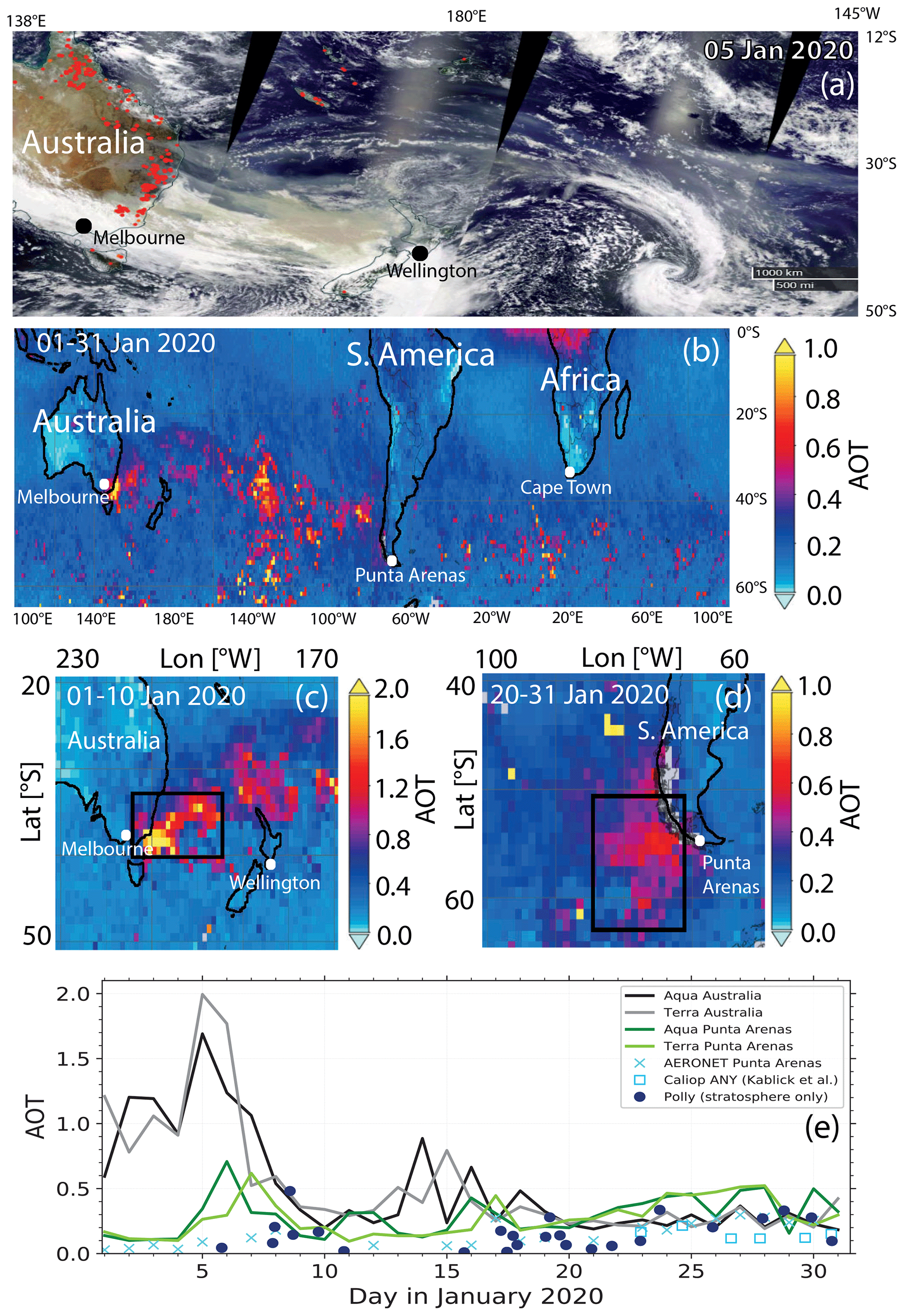
Figure 1Satellite observations of the stratospheric smoke transport from Australia to South America in January 2020. (a) Brownish smoke layer between Melbourne and Wellington on 5 January 2020 (MODIS, 2021a, b) and fires indicated by red spots in eastern and northern Australia (FIRMS, 2021). (b) The 500 nm AOT in the Southern Hemisphere (MODIS, 2021c); the smoke plumes were traveling mostly eastward. (c) Mean AOT values for the 1–10 January period, close to the source region (MODIS, 2021c). (d) Mean AOT values for the 20–31 January period, close to southern South America (MODIS, 2021c). (e) Time series of daily 500 nm AOT (mean values for the black rectangles are shown in (c) and (d) separately for MODIS Terra and Aqua). Cloud-screened values are shown (MODIS, 2021c). In addition, AERONET sun photometer values of the total (tropospheric + stratospheric) AOT at Punta Arenas, CALIOP-derived AOT values, as shown in Kablick et al. (2020), for the multiday outbreak ANY (Australian New Year), and Polly AOT values for the stratosphere over Punta Arenas, are shown.
Figure 1e provides a time series of daily AOT observed with MODIS (Terra and Aqua satellites), an AERONET photometer, and lidar at Punta Arenas. Initially, the area mean AOT values were close to 2.0 in the black rectangle shown in Fig. 1c and then mostly in the range from 0.2 to 0.5 after 10 January 2020. According to the time series of daily cloud-screened MODIS AOT observations within the black rectangle in Fig. 1d, the rotating smoke-filled vortex close to Punta Arenas caused AOTs of 0.3–0.5 during the last week of January 2020. Details of the rotating smoke fields are given in the next subsection. Note that the Southern Ocean AOT of the clean marine troposphere is of the order of 0.03–0.05 at 500 nm, as indicated by the Punta Arenas AERONET sun photometer observations from 1–6 January 2020.
Nighttime Raman lidar observations of 532 nm extinction profiles are used in Fig. 1e to compute the lidar-derived stratospheric AOTs. First, smoke plumes reached Punta Arenas on 5–7 January 2020. Significantly enhanced stratospheric AOTs were then observed on 8 January 2020 (Ohneiser et al., 2020). AOT values observed with lidar (during nighttime) and a photometer (during daytime) slowly increased towards values around 0.3–0.35 in the last week of January 2020. A few values measured with CALIOP during smoke vortex overflights (close to South America) from 23–31 January 2020 are included in Fig. 1e.
3.1.1 The unique, self-organized, rotating and ascending smoke-filled vortex
A new atmospheric phenomenon was detected in January–March 2020 (Kablick et al., 2020; Khaykin et al., 2020; Allen et al., 2020; Lestrelin et al., 2021). It coupled smoke occurrence, aerosol–radiation interaction, and dynamical processes. The striking discovery was the observation of several stratospheric smoke plumes that self-organized as quasi-ellipsoidal anticyclonic vortices, persisted over weeks to months, and traveled around the Southern Hemisphere. These plumes transported smoke up to heights above 30 km. The most intense, self-maintained vortex measured about 1000 km in diameter and about 5 km in vertical extent. This highly stable vortex persisted in the stratosphere for over 13 weeks, crossed the Pacific within 2 weeks, and hovered above the tip of South America for more than a week. It then followed a 10-week westbound round-the-world journey that could be tracked over 66 000 km until the beginning of April 2020 (Khaykin et al., 2020). The vortex lofted a confined bubble of smoke and moisture to 35 km altitude (Khaykin et al., 2020), an altitude not reached by tropospheric aerosols since the Pinatubo eruption (McCormick et al., 1995; Stenchikov et al., 2021). Aerosol heating was essential in maintaining the structure and providing the loft. In turn, the vortex created a confinement that preserved the embedded smoke cloud from being rapidly diluted within the environment (Lestrelin et al., 2021). Allen et al. (2020) emphasized that the peculiar motion was related to the steady rise in plume potential temperature of about 8 in January and 6 K d−1 in February, due to local heating by smoke absorption of solar radiation. This heating resulted in an anticyclonic (i.e., counterclockwise) circulation, with winds rotating around the plume at about 15 m s−1 (Kablick et al., 2020). Kablick et al. (2020) highlighted the importance of this detection. This is the first evidence of smoke causing changes to winds in the stratosphere and opens up a whole new vein of scientific research.
The rotating smoke field stayed close to the southernmost tip of South America (see also Fig. 1d) for 10–12 d, until the beginning of February 2020, and ascended by about 500 m d−1. During the steady and monotonic ascent, the smoke reached heights with dominating easterly winds. The center of the vortex was closest to Punta Arenas on 29–30 January 2020.
Figure 2a shows the disk-like structure southwest of the two lidar stations at Punta Arenas and Río Grande. The Sentinel-5 UV aerosol index from 340 and 388 nm is shown for 26 January 2020 (Sentinel-5, 2021). Bright blue colors indicate the presence of absorbing aerosol. The smoke plume was well captured by CALIPSO lidar observation on 25 January 2020, as shown in Fig. 2b (dashed curve in Fig. 2a shows the CALIOP track). The smoke vortex was detected between 19 and 26 km height at latitudes from 52 to 65∘ S.

Figure 2(a) Sentinel-5 aerosol index (340–380 nm), showing the location of the rotating and ascending smoke vortex southwest of the southernmost tip of South America on 26 January 2020 from 00:00 to 20:00 UTC (Sentinel-5, 2021). Indicated are the two ground-based lidar stations at Punta Arenas and Río Grande (white triangles). The white dashed line indicates the CALIOP overpass. (b) CALIOP observation along the overpass track on 25 January 2020 between 05:50 and 06:02 UTC, showing smoke plumes above 20 km and the smoke-filled vortex at latitudes south of 52.5∘ S in terms of the 532 nm attenuated backscatter coefficient. The thin vertical line at 52.3∘ indicates the shortest distance to the two ground-based lidars (triangles in panel a).
According to the Punta Arenas lidar observations in Fig. 3, parts of the rotating smoke field covered southern Chile from 24–31 January 2020. The flat base of the dome-like plume structure (see Fig. 2b) ascended from 19 km on 24 January to 22 km on 30 January and thus with a speed of about 500 m d−1 over the Polly lidar site. This is in agreement with the CALIOP observations shown in Khaykin et al. (2020), who found that the initial ascent rate was at 0.45 km d−1, with an average rate of 0.2 km d−1 for the 3-month period during which this smoke field existed.
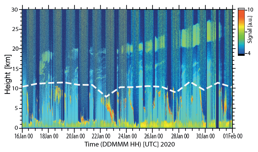
Figure 3The rotating and ascending smoke vortex, as observed with ground-based lidar at Punta Arenas from 24–31 January 2020. Shown is the range-corrected signal at 1064 nm wavelength in arbitrary units in a logarithmic color scale. The tropopause is indicated by the white dashed line. Tropospheric clouds and day and night signal background changes caused the many interruptions in the high-quality observations of the stratospheric smoke.
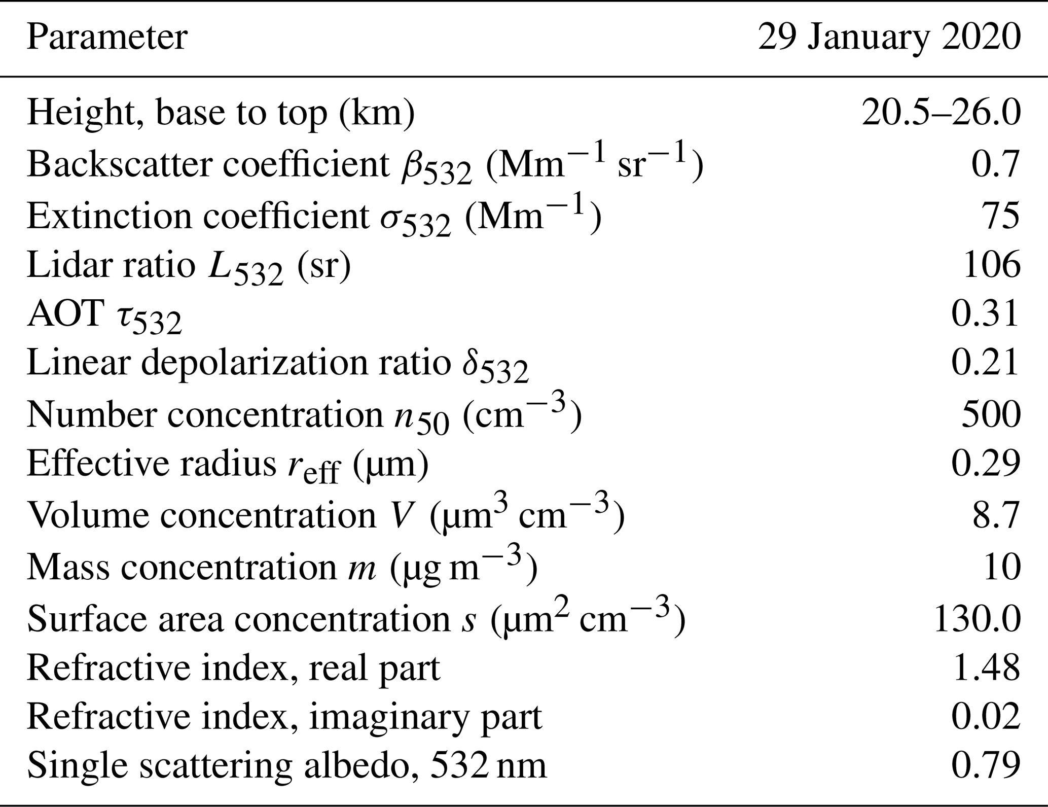
We performed a detailed analysis of the Punta Arenas lidar observations on 29 January 2020 when the vortex center was closest to the Polly lidar site. Table 1 summarizes the essential optical and microphysical properties, as discussed in detail by Ansmann et al. (2021a). The very large 532 nm lidar ratio of 106 sr that is also supported by the AERONET (AERONET, 2021) measurements used in Fig. 8 points to strongly light-absorbing smoke particles. The mass, volume, surface area, and number concentrations indicate a strong perturbation of the usually rather clean stratosphere. At unperturbed conditions, particle extinction coefficients are of the order of 0.1 Mm−1 (Sakai et al., 2016), particle surface area concentrations are in the range of 0.5–1 µm2 cm−3 (Hofmann and Solomon, 1989; Deshler et al., 2003), and particle number concentrations are around 5–10 cm−3. Now we found the particle number concentrations up to 500 cm−3, surface area concentrations of >100 µm2 cm−3, high mass concentrations (>10 µg cm−3), and 532 nm extinction coefficients of 75 Mm−1 in the layer from the 20–26 km height. The smoke volume size distributions for the Australian smoke, presented in Ansmann et al. (2021b) and Ohneiser et al. (2021), showed a pronounced accumulation mode (particles with radius mostly from 150–700 nm) with an effective radius of 280–300 nm. The revealed refractive index values, and the low single scattering albedo of close to 0.8 at all three wavelengths (not listed in the table) again points to strongly light-absorbing particles.
Table 1Layer mean particle optical (532 nm) properties and estimated microphysical properties of the rotating and ascending smoke disk on 29 January 2020, when the center of the vortex was close to Punta Arenas (Ohneiser et al., 2020; Ansmann et al., 2021a). Besides values obtained by the conversion of extinction coefficients into microphysical properties (Ansmann et al., 2021a), the lidar inversion method was applied to Polly multiwavelength backscatter and extinction observations on 26 January (Veselovskii et al., 2002) to add values for the effective radius, refractive index, and single scattering albedo. Uncertainties are of the order of 15 %–30 % in the optical properties and 20 %–50 % in the microphysical properties. We used values of ±0.1 for the real part of the refractive index, within an order of magnitude for the imaginary part, and ±0.05 for the single scattering albedo. The number concentration n50 considers particles with radius >50 nm only.
As discussed by Ohneiser et al. (2020), the lidar ratios for Australian smoke at 532 nm were considerably higher than the ones for Canadian smoke observed in August 2017 of 60–80 sr (Haarig et al., 2018). The difference is probably related to the different burning material. Australian's forests mainly consist of eucalyptus trees, whereas western Canadian tree types are predominantly pine, fir, aspen, and cedar.
3.2 Case studies from January 2020: optical fingerprints of aged wildfire smoke
To provide an overview of the basic lidar products, we begin with two case studies presented in Figs. 4 and 5. The Polly lidar monitored the smoke layers in terms of particle backscatter coefficients at three wavelengths and the particle extinction coefficient, lidar ratio, and depolarization ratio at two wavelengths. This set of optical properties allows us to characterize the smoke in large detail. However, the Polly instrument is optimized for tropospheric aerosol monitoring up to 10–12 km height, so that the extinction and lidar-ratio profiling was already at its limit for heights above 14 km, especially in the case of the measurement wavelengths of 355 and 387 nm for which the signal attenuation by Rayleigh scattering is strong and signal quality therefore quickly becomes low with height. On the other hand, the powerful CORAL instrument was optimized for stratospheric and lower mesospheric observations up to 90 km height and thus shows good performance at greater heights, as demonstrated in Fig. 5. Unfortunately, the minimum measurement height of CORAL is about 15 km, which makes direct comparisons with the Polly observations problematic.
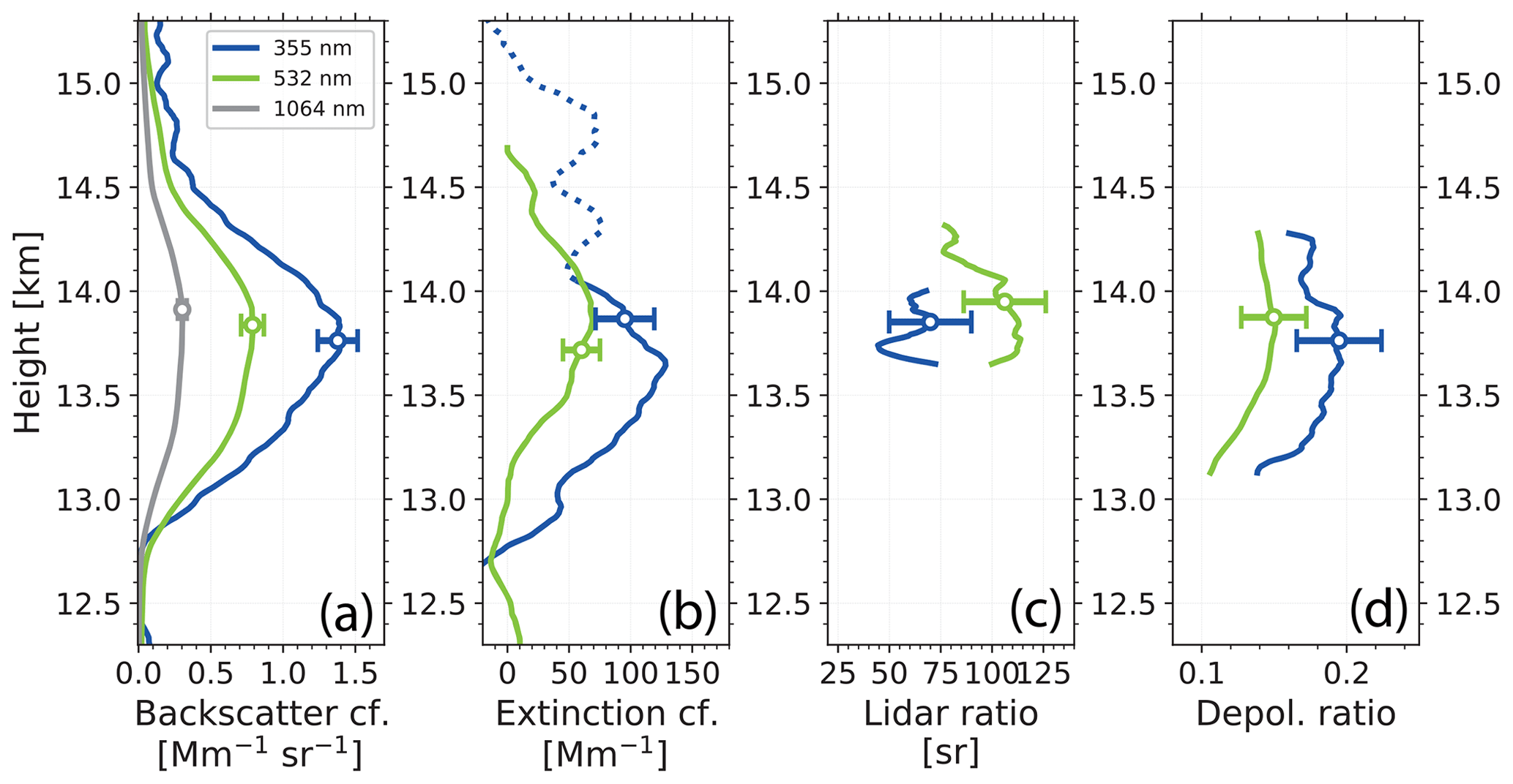
Figure 4Profiles of smoke optical properties measured with Polly over Punta Arenas on 8 January 2020 between 06:45 and 07:42 UTC. (a) Particle backscatter coefficient at three wavelengths, (b) smoke extinction coefficient, (c) smoke extinction-to-backscatter ratio (lidar ratio), and (d) particle linear depolarization ratio. Error bars show the estimated uncertainties. Profiles of backscatter (in panel a) and depolarization ratio (in panel d) were vertically smoothed with 500–700 m signal smoothing length, and the profiles of extinction coefficient (in panel b) and lidar ratio (in panel c) are obtained with a regression window length of 2–2.5 km. The dotted part of the 355 nm extinction profile indicates that the basic Raman lidar signals were too noisy to allow an accurate determination of the 355 nm extinction coefficient at heights above the layer center.
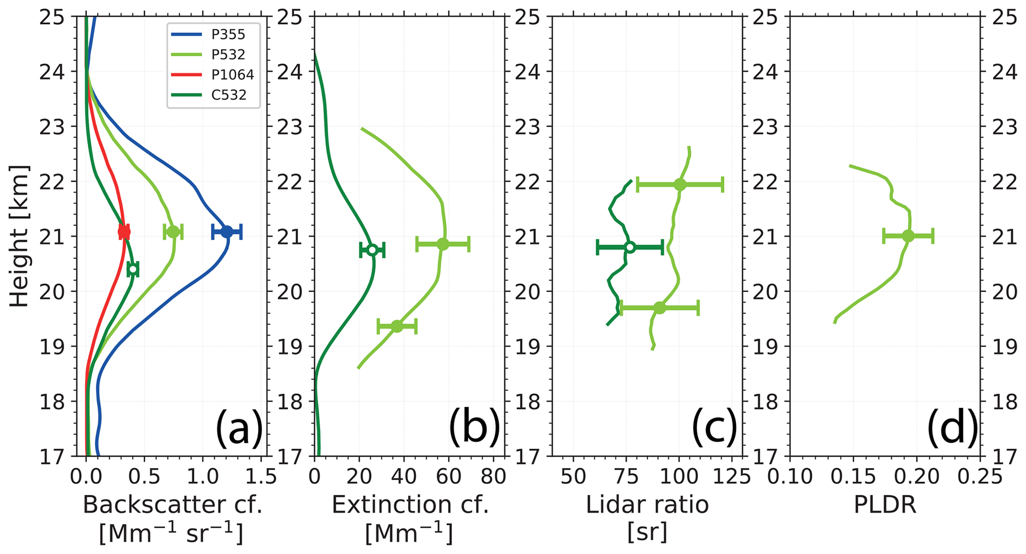
Figure 5Profiles of smoke optical properties measured with Polly (P; closed circles) over Punta Arenas and with CORAL (C; open olive circles) over Río Grande on 26 January 2020 between 04:27–06:18 (Polly) and 06:14–08:02 UTC (CORAL). (a) Particle backscatter coefficient at three wavelengths, (b) smoke extinction coefficient, (c) smoke extinction-to-backscatter ratio (lidar ratio), and (d) particle linear depolarization ratio (panels b–d at 532 nm). Error bars show the estimated uncertainties. Smoothing and regression window lengths are 500 m (Polly, backscatter, and depolarization) and 2 km (Polly, extinction, and lidar ratio). The 2 km smoothing and regression window lengths are used in the case of all CORAL profiles.
The measurements shown in Fig. 4 were performed when the first strong smoke plumes reached southern South America (Ohneiser et al., 2020). The maximum backscatter and extinction values were found at around 13–14.5 km height, and the layer base and top were at 12.7 and 14.7 km, respectively. The maximum extinction coefficients in the center of the smoke layer were around 70 Mm−1 at 532 nm and 120 Mm−1 at 355 nm. For the applied signal smoothing length of 2000–2500 m, the lidar ratios are fully trustworthy around the layer center only, as shown in Fig. 4. The 532 nm AOT was 0.08. The enhanced particle depolarization ratios of about 0.2 (355 nm) and 0.15 (532 nm) are clear indications for wildfire smoke reaching the stratosphere via fast pyroCb lofting (Haarig et al., 2018; Ohneiser et al., 2020).
In Fig. 5, the Polly and CORAL measurements are compared. The lidar observations on 26 January 2020 were performed close to the edge of the rotating and ascending smoke-filled vortex. The two lidars (230 km apart from each other) saw different parts of the horizontally inhomogeneous smoke field. This explains the differences in the 532 nm backscatter, extinction, and lidar ratio values. Stratospheric AOTs at 532 nm were 0.16 (Punta Arenas) and close to 0.05 (Río Grande).
Based on Figs. 4 and 5, we can summarize the following optical fingerprints of aged wildfire smoke. This aerosol type shows a clear wavelength dependence of the particle backscatter coefficient and a less pronounced spectral dependence of the extinction coefficient. Consequently, the extinction-to-backscatter ratio shows an inverse spectral behavior. The 532 nm lidar ratios are considerably larger than the 355 nm lidar ratios. Furthermore, the 532 nm lidar ratios typically exceed 70 sr and can be even larger than 100 sr. The CORAL observations yielded lidar ratios in the range from 65–85 sr on 5 different days in January and February 2020, but there was also a case with 100 sr on 16 January 2020. As mentioned already, the depolarization ratio of, typically, 0.15–0.2 at 532 nm and 0.2–0.25 at 355 nm are clear indications for smoke that was lofted into the stratosphere via strong pyroCb convection, i.e., within a rather short time period so that the morphological properties of the injected irregularly shaped carbonaceous particles remained widely unchanged when the particles entered the dry stratosphere. Only a small fraction of the smoke serves as cloud condensation nuclei and/or ice-nucleating particles, and the lack of significant precipitation produced in these cloud towers implies that only a small fraction of the smoke is scavenged so that most of it is exhausted through the anvil to the upper troposphere and lower stratosphere (Rosenfeld et al., 2007).
3.3 The decay phase: observation over 2 years (2020–2021)
Figure 6 provides an overview of the stratospheric perturbation from January 2020 to November 2021, as observed with the two ground-based lidars. One set of lidar products per day is considered. Gaps in the data time series are caused by fog and low-cloud events and by instrumental problems (long gap in July 2021). In the case of the CORAL observations, the laser stopped working properly in January 2021. Fortunately, these observations cover the main phase of the major stratospheric perturbation. Because of the designed lidar configuration, CORAL provided data for heights >15 km only.
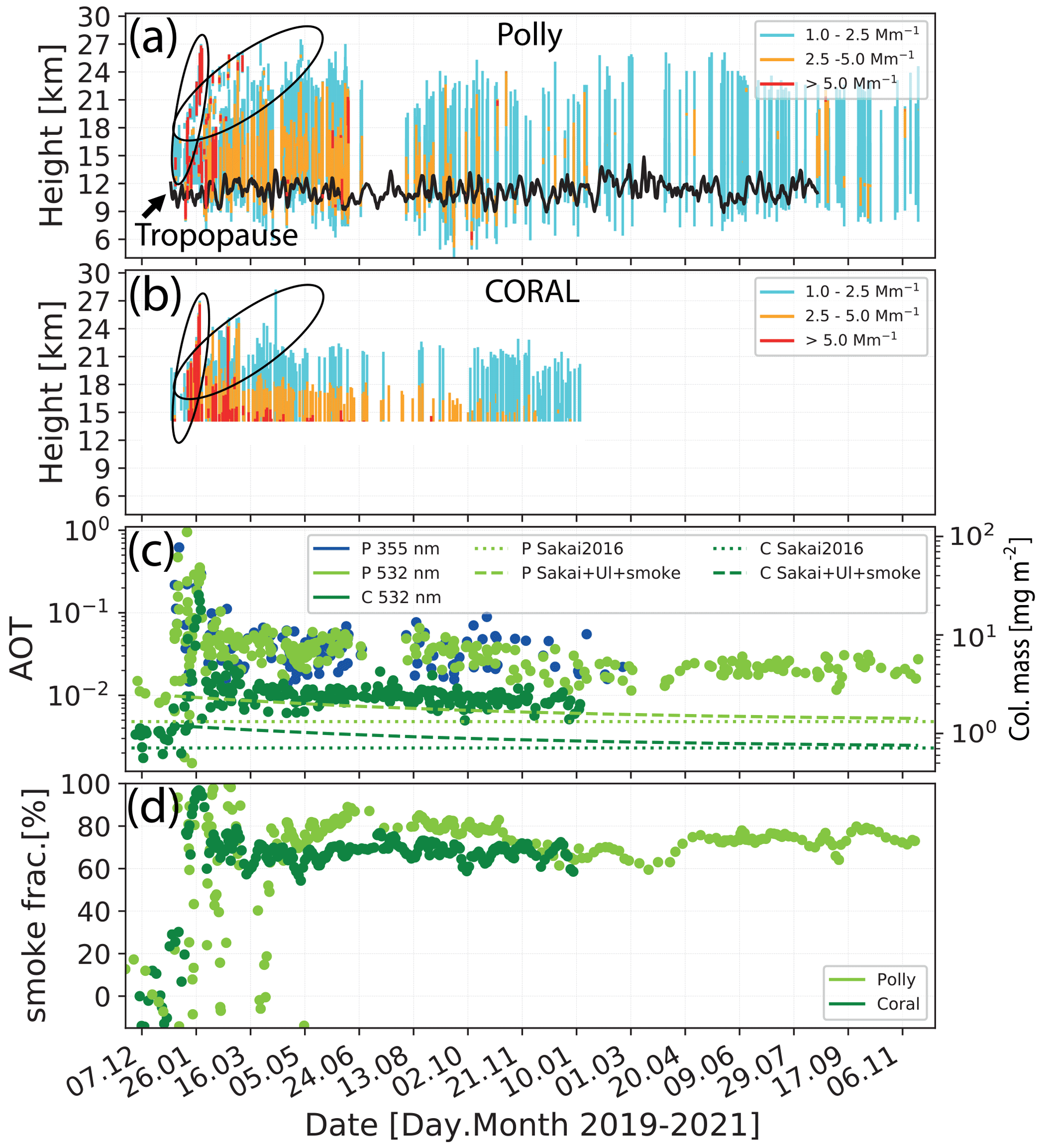
Figure 6(a) Overview of Polly observations of the UTLS smoke layers (colored bars from layer base to top; one bar per day) from 15 November 2019 to 15 November 2021. Observational gaps between bars are caused by periods with opaque clouds or instrumental problems. The colors in each bar indicate height segments with different 532 nm extinction coefficient levels (see the legend in the panel). Black oval circles highlight periods with frequently detected ascending layers. Panel (b) is the same as panel (a) except for CORAL observations at 532 nm with a minimum measurement height of 14 km. (c) Smoke layer AOT (C denotes CORAL; P denotes Polly) at 355 and 532 nm, calculated from the daily profiles of the particle backscatter coefficient and multiplied by a lidar ratio of 55 sr (355 nm) and 85 sr (532 nm). The Polly instrument measures the total UTLS smoke AOT and the CORAL system measures the AOT between 15 and 28 km. (d) Smoke contribution to total AOT, which includes contributions by the stratospheric background aerosol (dotted lines; Sakai et al., 2016), by Ulawun volcanic aerosol (Ul), and by Australian smoke reaching the stratosphere from September to December 2019 (smoke). The Ulawun and 2019 smoke contributions decreased with time (dashed curves; see the text for more details). Fluctuations in the smoke fraction around 0 that are visible until May 2020 are caused by measurement noise.
In Fig. 6a and b, layer height, depth, and particle light extinction information at 355 and 532 nm is given. We determined the layer base and top heights by visual inspection. In the case of Polly, the mean height profile of the 1064 nm backscatter coefficient was used, which is rather sensitive to particle backscattering. The base height is defined as the altitude at which the 1064 nm backscatter coefficient started to increase in the middle to upper troposphere after a minimum in the lower to middle free troposphere. The layer top was set to the height where the total-to-Rayleigh backscatter ratio at 1064 nm dropped below a value of 1.1. A similar approach was applied to the elastic backscatter signals, measured with CORAL at 532 nm, to determine the smoke layer top. The vertical bars in Figs. 6a and b are colored to distinguish different levels of the aerosol loading expressed in terms of the particle extinction coefficient. The backscatter coefficients at 532 nm were multiplied by a lidar ratio of 85 sr to obtain the extinction coefficients. A lidar ratio of 85 sr represents the mean extinction-to-backscatter relationship of the entire Australian smoke data set well. The tropopause is given in Fig. 6a to indicate that smoke was also present in the upper troposphere and influenced cirrus formation (Knopf et al., 2018; Ansmann et al., 2021a; Engelmann et al., 2021). After the injection of the first aerosol layers in January 2020, the smoke layers typically extended from 8–10 km height up to 21–25 km for the next 2 years. On average, the layer base and top heights were at 9.8 and 22.5 km, respectively. No long-term trend in the layer geometrical properties is visible. The optically densest part was found between 12 and 18 km height. The light extinction values slowly decreased with time (from red to orange to blue Fig. 6a and b). The periods with isolated, probably rotating and ascending, smoke-filled vortices are highlighted by big oval circles. Isolated smoke features vanished at the beginning of May 2020 (4 months after the ANYSO smoke injection period).
Figure 6c presents the time series of 532 nm AOT measured at Punta Arenas over the 2-year period. The AOT values were obtained by integrating the extinction values, i.e., the backscatter values multiplied with 85 sr, from the layer base to the top. The directly determined extinction coefficients (from the Raman signal profiles) were too noisy, and in many cases even not available for the upper part the smoke layers, and thus did not permit a trustworthy computation of the AOT time series for the 2-year period. The 355 nm AOT values in Fig. 6c were obtained from the 355 nm backscatter coefficients multiplied with a lidar ratio of 55 sr. Most of the variability in the 355 nm AOTs is caused by signal noise. The almost noise-free 532 nm AOT from the CORAL observations between 15 km and smoke layer top is given in Fig. 6c as well. A strong increase in the 532 nm AOT from November–December 2019 to January 2020 and large variability in AOT were found in January 2020 with the two lidars. The AOT reached values up to 1.0 at 532 nm in mid-January over Punta Arenas. The day-by-day AOT variability significantly decreased in February 2020. Since then, a slow and persistent decrease of the stratospheric perturbation has been visible. The AOT values at 532 nm decreased to 0.03–0.06 (February–June 2020), 0.02–0.05 (July–December 2020), and were about 0.015–0.03 in 2021. The AOT for undisturbed, clean stratospheric background conditions for the height range from the tropopause to 30 km height is about 0.005.
The contribution of Australian smoke to the total AOT is shown in Fig. 6d. The total AOT also includes contributions by Australian smoke reaching the stratosphere from September–December 2019, Ulawun volcanic aerosol, and background particles. In order to determine the smoke fraction caused by the ANYSO smoke injections, we need thus to consider the natural stratospheric background conditions and further contributions by aerosols injected in 2019 (Kloss et al., 2021a, b). In Fig. 6c, different stratospheric background levels for the wavelength of 532 nm are shown as dotted and dashed lines. In November–December 2019, UTLS AOTs around 0.01 (8–30 km height) and stratospheric AOTs around 0.004 (15–30 km height) were observed with the lidars at Punta Arenas and Río Grande, respectively, and in reasonable agreement with results from passive remote sensing for heights >15 km (Kloss et al., 2021b). According to Sakai et al. (2016), who analyzed Japanese lidar observations at Lauder, New Zealand, from 1992 to 2015, the minimum stratospheric background level is reflected in a 532 nm AOT of 0.0025 for the height range from 15–30 km height. The AOT is obtained from the measured minimum column-integrated backscatter coefficient multiplied by a lidar ratio for sulfate aerosol of 50 sr. This minimum background level (for the 15–30 km height range) is indicated by a dark green line in Fig. 6c. From the New Zealand lidar observations, it can be concluded that the UTLS AOT is roughly 0.005 during clean conditions (light green dotted line in Fig. 6c). This estimate was found to be in agreement with the analysis of satellite observations from 1990 to 2010 during volcanic quiescent times (Solomon et al., 2011).
However, further contributions to the AOT measured in November–December 2019 need to be added. The Ulawun volcano in Papua New Guinea (5∘ S, 151∘ E) erupted on 26 June 2019 (injection of 0.14 Tg SO2 into the stratosphere) and on 3–4 August 2019 (injection of 0.3 Tg SO2; Kloss et al., 2021a) and most probably caused a stratospheric AOT at 532 nm of around 0.005 at the end of September 2019 and of 0.0025 2–3 months later. We estimated the Ulawun-related AOT by comparing SO2 emissions and the resulting stratospheric sulfate AOT for the Raikoke, Sarychev, and Ulawun eruptions (Haywood et al., 2010; Kloss et al., 2021a, b; Ohneiser et al., 2021). For the height range >15 km, we arbitrarily assumed a volcanic AOT contribution of 0.001 for the November–December 2019 period. To realistically consider the decrease in the Ulawun-related disturbance of the stratospheric aerosol conditions, we assumed a decay time of 180 d.
As a second additional contribution Kloss et al. (2021b) identified Australian smoke emitted from September to December 2019. To match the measured AOT values of 0.005 and 0.01 over Río Grande and Punta Arenas, respectively, this contribution must also have been of the order of 0.0025 (for the UTLS height range) and 0.001 (for the height range >15 km). Here, we assume a decay time of 1 year (365 d). The sum of all three contributions (constant minimum background level plus volcanic AOT plus Australian smoke for the September to December period) is shown as dashed lines in Fig. 6c. By considering these enhanced time-dependent background levels, we can conclude that the ANYSO smoke caused roughly a factor of 4 higher stratospheric AOT values over the midlatitudes in the Southern Hemisphere for more than 1 year. Accordingly, the ANYSO smoke fraction for the UTLS height range, shown in Fig. 6d, was about 80 % during 2020 and 70 %–80 % in 2021. On the contrary, the Ulawun-related AOT fraction was about 25 % in November–December 2019, negligible in January 2020, about 5 % in February–April 2020, and <3 % as of June 2020.
In Fig. 7, the stratospheric aerosol perturbation in 2020 and 2021 is presented as a function of height. Besides the January 2020 mean extinction profile (in red), the February–June 2020 mean profile (orange), and further three half-year mean extinction profiles (blue, green, and black) are shown together with the pre-ANYSO 532 nm extinction profile (November–December 2019 in dark gray). The daily height profiles of the particle backscatter coefficient at 532 nm were multiplied by a representative smoke lidar ratio of 85 sr and then separately averaged for the different time periods. In the case of the November and December 2019 backscatter height profiles (pre-ANYSO profiles), we applied a lidar ratio of 60 sr to consider the contribution of volcanic aerosol (lidar ratio of 45 sr) and stratospheric background aerosol (lidar ratio of 50 sr) in addition to the September–December 2019 smoke from Australia (lidar ratio of 85 sr). The dashed lines in Fig. 7a above approximately 25 km height are calculated by applying the Klett method to the strong elastic backscatter signals (Fernald, 1984), as described in Sect. 2.1. The stratospheric minimum background extinction levels (Sakai et al., 2016) are given as well in Fig. 7 as a thin solid dotted gray line.
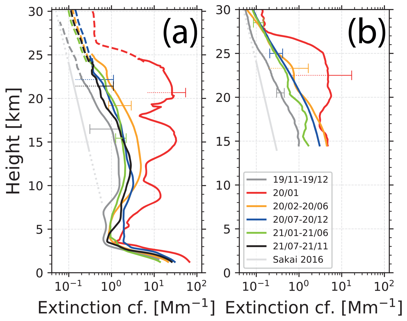
Figure 7January 2020 mean (red), February–June 2020 mean (orange), and half-year mean profiles of smoke extinction coefficient at 532 nm. (a) Polly observation (1–30 km). (b) CORAL (15-30 km). The particle extinction coefficients were retrieved by multiplying the backscatter coefficient profiles by 85 sr. All solid profiles are average profiles calculated with the Raman lidar method. The bars indicate 1 standard deviation caused by atmospheric variability. Dotted parts indicate bars ending at values <0.03 Mm−1, i.e., outside the frame. The dashed lines in panel (a) were calculated with the Fernald method (as explained in Sect. 2.1). The thin, solid dotted gray lines show stratospheric background values (Sakai et al., 2016). The November–December 2019 mean extinction profile (before the ANYSO event) is given as dark gray curve, here a lidar ratio of 60 sr is used to convert backscatter into extinction values.
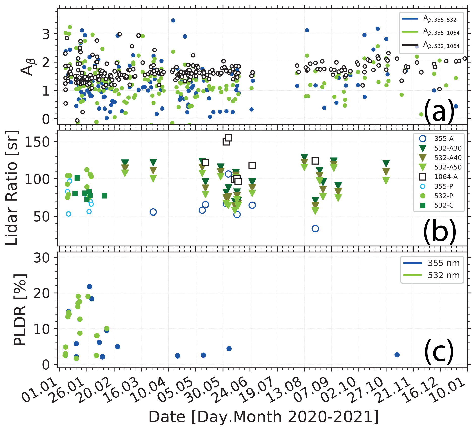
Figure 8Smoke layer mean optical properties (daily values) observed from 1 January 2020 to 10 January 2021. (a) Backscatter-related Ångström exponent Aβ. (b) Extinction-to-backscatter ratio (lidar ratio) from Polly (P) and CORAL (C) measurements in January–February 2020 and from combined lidar–AERONET observations (since March 2020) by using lidar ratios of 30 (A30), 40 (A and A40), and 50 sr (A50) in the estimation of the tropospheric 532 nm AOT from lidar observations (see the text for a further explanation). Stratospheric lidar ratios at 355 nm (circles) and 1064 nm (squares) are shown for a lidar ratio of 40 sr in the tropospheric AOT retrieval. (c) Particle linear depolarization ratio (PLDR). The scatter in the data is mainly caused by signal noise and to a minor degree by atmospheric variability.
The extinction profile in November–December 2019 indicates already significantly enhanced aerosol pollution levels that have been caused by the Australian fires since September 2019 (Kloss et al., 2021b) and volcanic sulfate aerosol (Ulawun eruption; Kloss et al., 2021a). Then, in January 2020, the aerosol extinction coefficient increased by 1–2 orders of magnitude compared to the November–December 2019 extinction levels in the height range from 8–25 km and more than 2 orders of magnitude with respect to the minimum perturbation (Sakai et al., 2016). The structure of the January 2020 profile is dominated by the arrival of several single, very dense smoke layers, such as the rotating and ascending smoke-filled vortex in the last January week. Monthly mean extinction values of 10–30 Mm−1 were found in January 2020. The following half-year mean extinction profiles showed much lower values. However, these profiles indicate quite a slow decay of the perturbation from February 2020 to November 2021. In the second half of 2021, the extinction values were still a factor of 5–10 higher than the extinction levels representing a minimum stratospheric aerosol load (Sakai et al., 2016). Note also that the extinction levels were also clearly enhanced between 26 and 30 km height in 2020–2021.
3.4 Smoke intensive parameters
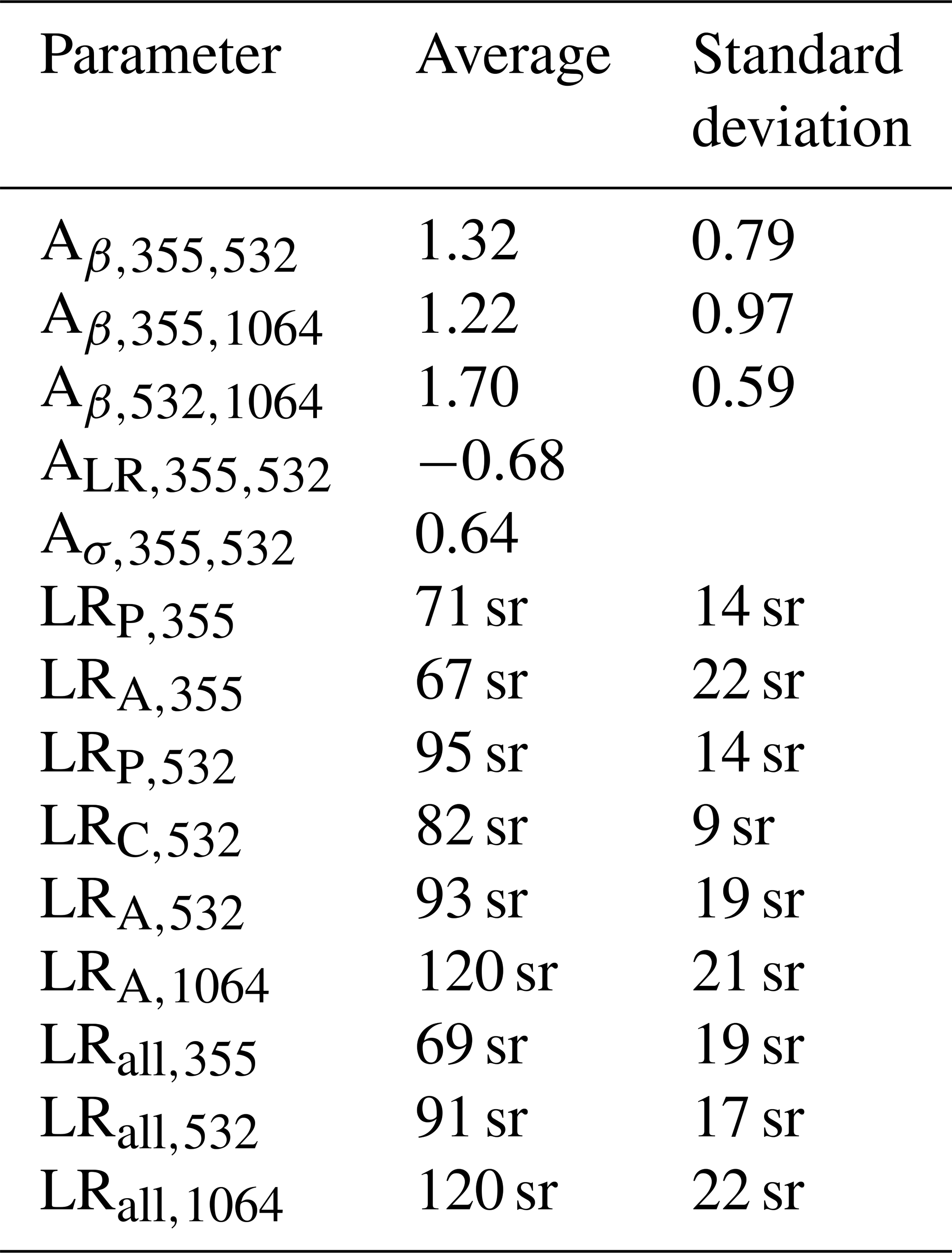
Figure 8 shows time series of smoke-intensive properties for the year 2020. The backscatter-related Ångström exponents (defined in Sect. 2.1), the extinction-to-backscatter ratio, and the particle linear depolarization ratio enable a good optical characterization of aged wildfire smoke. The strong variability in the data, especially in the case of the backscatter-related Ångström exponent for the short wavelength range (355–532 nm), is caused by signal noise rather than changes in the microphysical and chemical properties of the smoke particles. Mean values of the Ångström exponents and lidar ratios shown in Fig. 8 are given in Table 2. The statistics consider 326 values for each Ångström exponent, 7–10 values for each of the lidar ratios, except for the Polly–AERONET 532 nm lidar ratio (19 values). The PLDR statistics are based on 14 (355 nm) and 17 values (532 nm).
Table 2Mean values and standard deviations of the Ångström exponents (backscatter related, Aβ, lidar ratio related, ALR, and extinction related, Aσ) and lidar ratios (LR) computed from all stratospheric values shown in Fig 8. Lidar ratio index includes the following: A – AERONET–Polly retrieval; P – Polly observation; C – CORAL observation; all – mean values by considering all determined and retrieved LR values. The standard deviations include atmospheric variability and dominating retrieval uncertainties. A further explanation is given in the text.
As can be seen in Fig. 8a, the Ångström exponents for the 355–1064 nm and the 532–1064 nm wavelength ranges accumulated between 1 and 2. Such values were already observed in the stratosphere for aged Canadian smoke observed over central Europe in August 2017 (Haarig et al., 2018) and for aged Siberian smoke in the High Arctic (Ohneiser et al., 2021) and points to a pronounced accumulation-mode-dominated particle size distribution and the absence of a particle coarse mode. The less noisy Ångström exponent values for the long wavelength range (532–1064 nm) accumulate at around 1.5 in January 2020 and are around 1.8 in the second half of 2020. This increase reflects a shift in the size distribution towards smaller particles. Larger particles may have been removed by sedimentation processes.
Lidar ratios at 355 and 532 nm could be measured directly with the two lidars in January and February 2020 only (see Fig. 8b). The lidar ratios measured with Polly in January 2020 (blue and light green) are also given in Table 1 in Ohneiser et al. (2020). The values range from 50–100 sr (355 nm) and 75–115 sr (532 nm). The CORAL values for 532 nm in Fig. 8b accumulate around 80 sr. Since March 2020, the Raman signal profiles have been too noisy and the smoke extinction coefficients too low and have no longer allowed a lidar ratio retrieval. In order to obtain some snapshot-like estimates for the smoke lidar ratio at 355 and 532 nm, and even for the IR wavelength of 1064 nm, we combined stratospheric AOT estimates from AERONET sun photometer observations at 380, 500, and 1020 nm with respective lidar-derived stratospheric-column-integrated backscatter values at 355, 532, and 1064 nm. In this approach, we estimated the stratospheric AOT from the total (tropospheric + stratospheric) AOT measured the AERONET photometer at Punta Arenas during favorable, stable, and temporally constant aerosol conditions. We subtracted the tropospheric AOT contribution from these AERONET AOT values. The tropospheric AOT was estimated by using the tropospheric backscatter and extinction profiles (from the surface to the tropopause) obtained with the Fernald method that was applied to the elastic backscatter signal profiles (Fernald, 1984). We assumed reasonable tropospheric lidar ratios of 30, 40, and 50 sr for a mixture of continental and marine aerosols in the Fernald data analysis to obtain the tropospheric AOTs at 355, 532, and 1064 nm. We combined the lidar observations with the near-range and far-range telescope (receiver units) to obtain the full extinction profile from close to the ground up to the tropopause. In order to transfer the total (tropospheric + stratospheric) AERONET AOT values at 380, 500, and 1020 nm to the ones for the lidar wavelengths at 355, 532, and 1064 nm, we used climatologically mean tropospheric Ångström values measured over Punta Arenas during undisturbed stratospheric aerosol conditions from January to July 2019. The ratio of the stratospheric AOT (from the combined AERONET and Polly observations) to the respective stratospheric column backscatter coefficient is shown in Fig. 8b. The label 532-A40 indicates, e.g., the use of AERONET observations (index A) and the use of a lidar ratio of 40 sr (index 40) in the retrieval of the tropospheric AOT at 532 nm. In Fig. 8b, we only show smoke lidar ratio solutions for 355 and 1064 nm for the tropospheric lidar ratio assumption of 40 sr to avoid overloading the figure with too many results.
One should emphasize that these retrieved stratospheric lidar ratios must be regarded as rough estimates. In this combined AERONET–Polly approach, we ignore an underestimation of the stratospheric smoke AOT from AERONET sun photometer observations up to 20 %–30 %, as discussed by Ansmann et al. (2018). Furthermore, measurements with lidar and the photometer did not exactly cover the same time periods and thus may have been conducted at slightly different boundary layer, free tropospheric, and stratospheric aerosol conditions. Thus, the shown lidar ratios provide only a very general view on the spectral behavior of the smoke lidar ratios. Nevertheless, the findings are in line with previous observations (Haarig et al., 2018). When averaging all lidar ratios obtained with the different methods, the resulting lidar ratios are 69, 91, and 120 sr for 355, 532, and 1064 nm, respectively.
Table 2 summarizes the observations in Fig. 8a and b. With the mean lidar ratios of 69 and 91 sr, the lidar-ratio-related Ångström exponent ALR was calculated and also the extinction-related Ångström exponent Aσ with . The low values of Aσ and the negative value of ALR are clear optical fingerprints of wildfire smoke (Ohneiser et al., 2020; Haarig et al., 2018).
Figure 8c shows the evolution of the particle linear depolarization ratio (PLDR) at 355 and 532 nm. High-quality depolarization ratio observations were frequently only possible in the lower half of the smoke layer. The shown values may thus not be at all representative for the entire layer (from base to top). Initially, the PLDR showed values close to 20 % for fresh smoke in the stratosphere. In the first 2 months, the smoke PLDR was very variable, with values from almost 0 % to 20 %. After 2 months, the PLDR decreases to values below 5 %. After 3 months, only a few useful measurements were possible, and the PLDR values were below 5 % for both wavelengths. The smoke particles obviously became rather compact and spherical in shape within a short time of about 4–6 weeks. The depolarization ratios are further discussed in the next section.
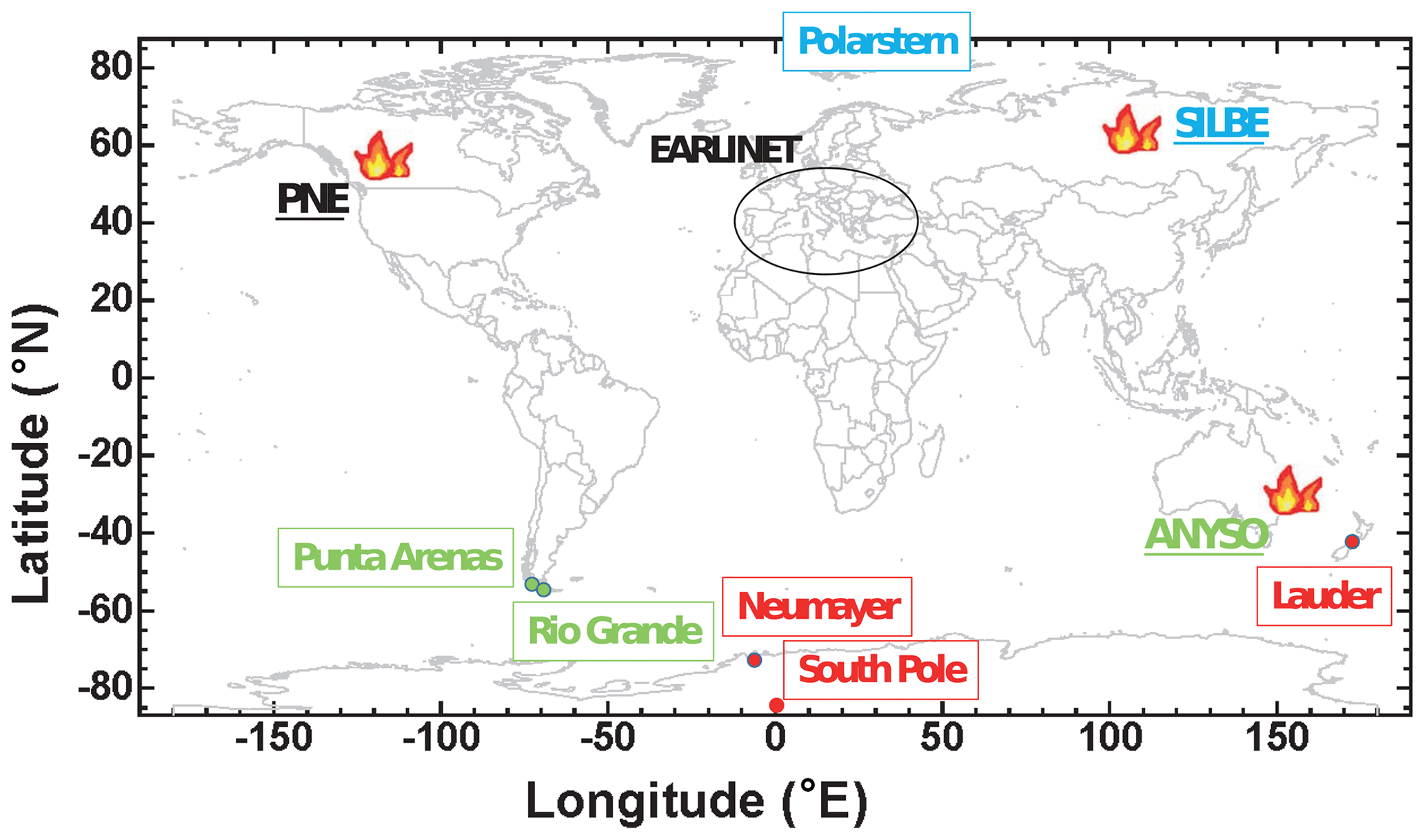
Figure 9Map showing the ground-based lidar stations at Punta Arenas (ANYSO smoke observations in 2020/2021), in the High Arctic (Polarstern, SILBE smoke observations in 2019/2020), in Europe (PNE smoke observations in 2017/2018). In addition, the ozonesonde stations at Lauder, New Zealand, at the Neumayer Station, and at the South Pole are indicated.
3.5 Comparison of three major stratospheric smoke events: ANYSO (2020) vs. PNE (2017) vs. SILBE (2019)
In this section, the decay behavior of the stratospheric perturbation caused by the Australian fire smoke is discussed in more detail. We use the opportunity to compare the ANYSO event with respective observations of two major smoke events occurring in the Northern Hemisphere in 2017 and 2019–2020 (see Fig. 9). The record-breaking Canadian fire storm (PNE, 2017) was already mentioned in Sect. 3.1. Strong smoke injection into the UTLS regime occurred during a cluster of about five pyroCb pulses over British Columbia, Canada, on 12–13 August 2017 (Peterson et al., 2018, 2021). Lidar network observations of aged smoke after long-range transport over weeks to months were conducted over Europe (indicated by a black circle in Fig. 9) from August 2017 to January 2018 (Baars et al., 2019). We further include lidar observations of the decay phase of a dense stratospheric smoke layer observed over the High Arctic with a Polly lidar aboard the ice breaker Polarstern. These observations, from October 2019 to May 2020, were performed in the framework of the MOSAiC (Multidisciplinary drifting Observatory for the Study of Arctic Climate) expedition (Engelmann et al., 2021; Ohneiser et al., 2021). Extremely strong fires occurred over central and eastern Siberia, north and northeast of Lake Baikal (SIberian Lake Baikal Event, SILBE), from mid-July to mid-August 2019. The fire smoke reached the UTLS height range, most probably by so-called self-lofting processes, within 2–7 d after injection into the lower troposphere (Ohneiser et al., 2021). The pyroCb activity was absent over the huge Siberian fire region in July and August 2019. Since there was an injection of Siberian smoke into the UTLS height range about 2500–3500 km south of the High Arctic, the plumes had to travel a short distance only with the prevailing westerly to southerly winds.
In Fig. 10, the three major stratospheric smoke events are compared regarding their geometrical and optical properties. As can be seen, the vertical extent of the Canadian smoke layers was of the order of 1–4 km, and these smoke layers were clearly observable over Europe with lidar up to 150 d after injection only. The Siberian smoke formed a 7–10 km thick layer and was monitored from day 80 up to about 300 d after injection. From December 2019 to May 2020, the smoke was trapped around the North Pole under the influence of a rather strong polar vortex. The stratospheric perturbation could be observed until the strong polar vortex collapsed in May 2020 so that the smoke became dispersed over a larger region towards the midlatitudes in the late spring and summer of 2020. The Australian fires were by far the strongest and produced a 10–15 km thick layer. These smoke layers were clearly detectable even 2 years after injection. Unfortunately, we had to stop the DACAPO-PESO campaign and thus our Punta Arenas smoke observation at the end of November 2021. The CORAL system, on the other hand, has been measuring again since December 2021.
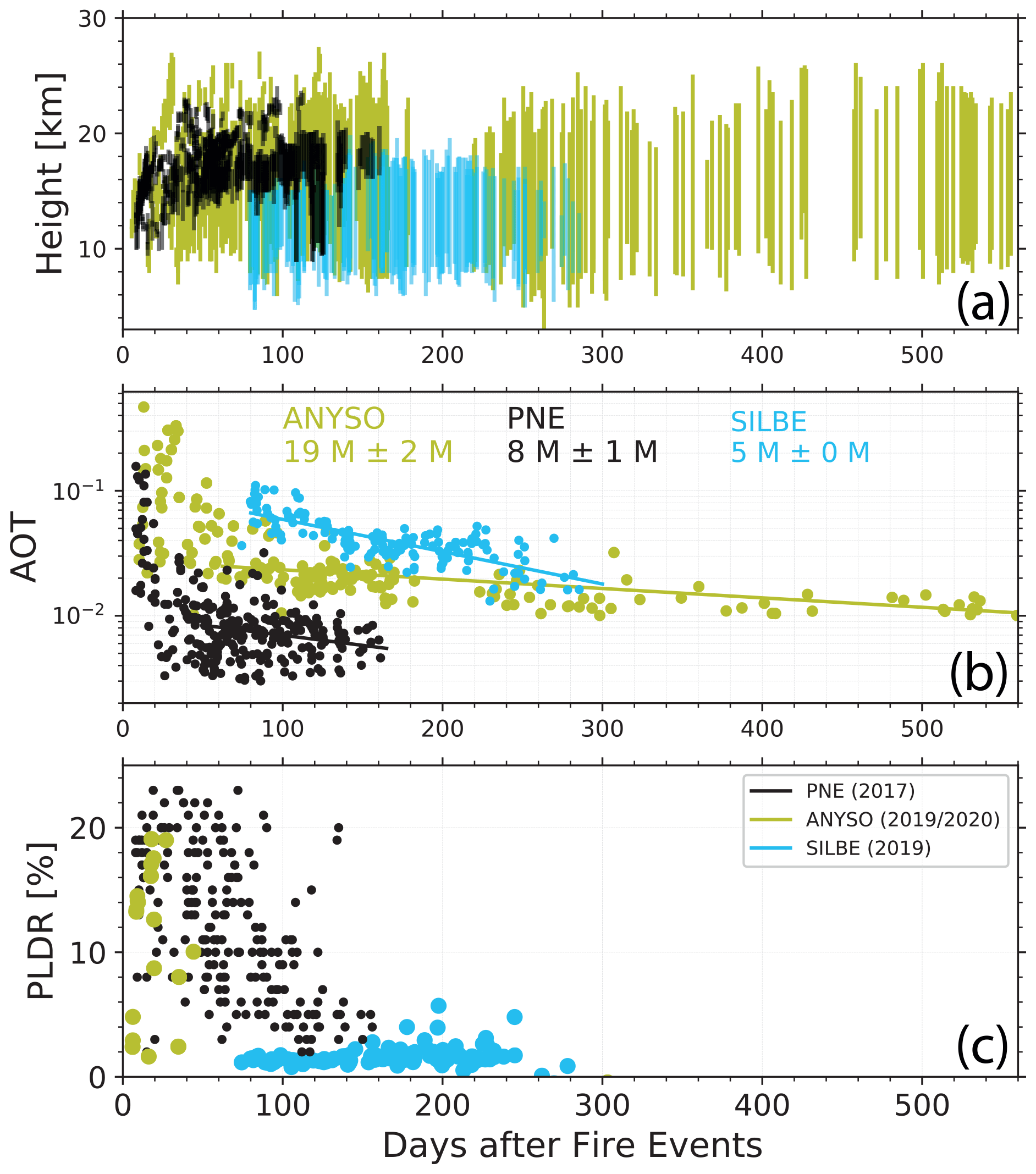
Figure 10Comparison of geometrical and optical properties of three stratospheric fire smoke events measured with different Polly instruments. Day 0 is the 12 August 2017 (PNE), 23 July 2019 (SILBE), and 31 December 2019 (ANYSO). Canadian (PNE) and Siberian (SILBE) fire smoke data are taken from Baars et al. (2019) and Ohneiser et al. (2021), respectively. (a) Overview of Polly observations of UTLS smoke layers (colored bars from layer base to top) in the days after smoke injection into the UTLS height regime. (b) The 532 nm AOT times series for the different wildfire events; straight lines indicate the decay of the perturbations according to the given e-folding decay times in months (M). In the case of PNE and ANYSO observations, AOT for heights >13 km is used. (c) Particle depolarization ratios (layer mean values at 532 nm) for the different fire events.
The layer base height of the ANYSO and SILBE smoke layers was always close to or slightly below the tropopause (mostly at 8–10 km height). In contrast, the base height of the PNE smoke layer was typically several kilometers above the tropopause. The top height was mostly around 20 (PNE), 18 (SILBE), and 23–24 km (ANYSO). The different top heights had a sensitive impact on the decay of the stratospheric perturbation described in terms of e-folding decay times.
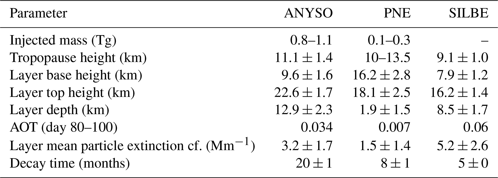
Table 3Comparison of the three wildfire smoke events (ANYSO – Australian fires; PNE – Canadian fires; SILBE – Siberian fires) in terms of mean values and SD of smoke layer geometrical and optical properties and perturbation decay time. The observations were performed over Europe (PNE), Punta Arenas (ANYSO), and the North Pole region (SILBE). For these sites and regions (see Fig. 9), the mean tropopause height and SD and, for Europe, the typical tropopause height range are given as well.
In Fig. 10b, the AOT data sets of the three wildfire events are compared, and the decay behavior of the different stratospheric perturbations are presented. As expected, the PNE AOTs were, on average, 3 to 4 times lower than the ANYSO AOTs (see the discussion in Sect. 3.1). In order to see a clear reduction in the AOT with time, the shown PNE and ANYSO AOTs were computed from the smoke extinction coefficients between 13 and 30 km height and thus for a height range several kilometers above the tropopause. The selection of the 13 km level as base height was necessary in the case of the ANYSO AOTs to avoid the impact of new aerosol plumes in 2020 and 2021 that regularly appeared in the tropopause region on the decay time computations. The decay behavior is indicated by straight lines in Fig. 10b. The respective e-folding decay times are given as numbers in Fig. 10b and were computed by using the AOT time series from day 40 to 160 (PNE) and from day 60 to 560 (ANYSO). The first 40–60 d (after smoke injection) were excluded because they showed a rather strong AOT variability and no clear trend.
The MOSAiC observations started about 80 d after the injection of the smoke into the UTLS regime so that a removal of strongly varying AOT values in the decay time calculations was not necessary in the case of the Siberian smoke. Furthermore, the entire smoke layer, from base to top, was considered in the AOT calculations. The impact of tropospheric aerosol sources on the smoke AOT evolution over the High Arctic was found to be negligible. In terms of the total AOT (from base to top layer), the ANYSO and SILBE smoke events were similar regarding the injected smoke amount and corresponding stratospheric AOTs.
Strong differences in the decay behavior of the stratospheric perturbation in the Northern and Southern hemispheres were found. A very large value of the e-folding decay time of 20 ± 2 months was obtained from the ANYSO AOT data set and a quite short decay time of 8 ± 1 months in the case of PNE (2017). If we remove the impact of the stratospheric background aerosol and Ulawun volcanic sulfate aerosol (shown in Fig. 6c), the ANYSO AOT decay time decreases to 19 ± 1 months. Several processes influence the decay time. Besides the sedimentation of particles and self-lofting of the absorbing smoke particle, horizontal (meridional) dispersion, and even the growth of the smoke particles by water uptake and condensation of gases on the particles have to be taken into account. Larger particles produce larger optical effects and thus lead to an increase in AOT.
The top height of the smoke layer plays an important role as well. The ANYSO smoke was distributed over the entire lower stratosphere up to heights around 24 km. And this comparably large top height in combination with particle sedimentation was responsible for the e-folding decay time of 19–20 months, as we will further discuss below. The PNE smoke was mostly confined between 14 and 20 km height and thus could be removed quite efficiently (from the stratosphere above 13 km). Furthermore, complex horizontal dispersion features in the Northern Hemisphere have been reported in the case of the Canadian smoke event (Kloss et al., 2019; Pumphrey et al., 2021). The smoke became efficiently distributed towards the tropics and towards the North Pole within a few weeks. On the other hand, a clear detection of the Canadian smoke was only possible until January–February 2018 (up to 5–6 months after injection), so that an accurate decay time could not be computed from such a short time series with quite strongly varying AOT values.
The short decay time for the High Arctic smoke (SILBE, 2019–2020) of 5 months is related to the specific polar meteorological conditions (impact of the strong polar vortex) and specific vertical air mass exchange mechanisms (related to the Brewer–Dobson circulation) and also to the fact that we considered the AOT from the layer base in the upper troposphere to the top at around 18 km height in the computation. Thus, even removal processes in the upper troposphere (e.g., by cirrus evolution and removal of smoke particles by falling ice crystals) had an impact on the decay behavior.
Table 3 summarized the key features for the three events and allows further comparison. It is worthwhile to also compare the ANYSO decay time with decay times of volcanic perturbations found after the Pinatubo eruption in 1991 at midlatitude lidar stations in the Northern and Southern hemispheres. The Pinatubo aerosol layer also reached about 25 km height. In the case of volcanic aerosol, the dominating removal process is sedimentation. Self-lofting and particle growth aspects can be ignored in the analysis of the decay of a volcanic perturbation 1–5 years after the eruption. For the Northern Hemisphere, our long-term lidar observations of the Pinatubo sulfate aerosol at Geesthacht (close to Hamburg) at 53.4∘ N in northern Germany, yielded decay times of 14–15 months (445 d; Ansmann et al., 1997). Nagai et al. (2010) reported e-folding decay times of 14 and 16.5 months obtained from lidar observations at Tsukuba (near Tokyo, 36.1∘ N), Japan, and Lauder (45∘ S), New Zealand, respectively. According to Sekiya et al. (2016), the Pinatubo-related decay time was 12–13-months on a global scale. Sekiya et al. (2016) performed a global-scale modeling constraint to the lidar observations at Tsukuba and Lauder. The shorter Pinatubo decay times are related to the fact that the volcanic sulfate particles showed a characteristic (effective) radius of 0.4–0.5 µm (Ansmann et al., 1997), whereas the Australian smoke particles were much smaller, with effective radii of 0.2–0.3 µm (Ansmann et al., 2021a), so that the sedimentation speed was much smaller. Self-lofting processes and particle growth effects had no impact on the decay behavior a few months after injection when the AOT was mostly <0.05.
In Fig. 10c, we finally compare the observed particle depolarization ratios of the three fire events. As can be seen, in the case of Canadian smoke over Europe (PNE, 2017), the depolarization ratio decreased slowly with time. This points to a slow smoke aging process in the dry stratosphere at low relative humidity conditions and low levels of condensable gases. It took several months before the initially irregularly shaped particles became very compact and, at the end, spherical so that the depolarization ratio approached values <0.05. The aging process seemed to be much faster in the Southern Hemisphere (ANYSO, 2020). A relatively large amount of water vapor and condensable gases was available in the stratosphere so that the smoke particles became spherical in shape within 4–6 weeks after injection. Khaykin et al. (2020) reported a remarkable increase in the stratospheric abundance of the gaseous combustion products which were injected together with the smoke aerosol. Furthermore, the injected mass of water was estimated to be very high (27 ± 10 Tg; about 3 % of the total mass of stratospheric overworld water vapor in the southern extratropics). Unfortunately, it was difficult to determine trustworthy particle depolarization ratios over Punta Arenas from February 2020 onwards. However, as shown in Fig. 8c, the few 355 nm depolarization ratios from March to June 2020 indicate the comparably fast decrease in the depolarization ratio with time and thus fast particle aging. All depolarization values in Fig. 8c were ≤10 % since February 2020.
In strong contrast to these pyroCb-related smoke events, the Siberian smoke (SILBE, 2019) showed a rather different behavior. Rather low depolarization ratio values were found at all sites after the beginning of the MOSAiC campaign in October 2019 (about 80 d after injection into the UTLS height range over Siberia). Lidar measurements of stratospheric smoke layers over Leipzig, Germany, in August 2019 (originating from the SILBE fires, according to backward trajectory analysis) and with CALIOP also revealed low smoke depolarization ratios (Ansmann et al., 2021b).
This strong contrast to the ANYSO and PNE depolarization features again points to the fact that different lofting processes took place. The pyroCb convection was responsible for the fast lofting of smoke towards stratospheric heights (within less than a few hours) in the case of PNE and ANYSO, so that emitted particles retained their irregular shape. On the other hand, a slow ascent over days caused by self-lofting prevailed in the case of SILBE smoke. The aging process could be completed within these few days so that the spherical shapes of the core shell particles dominated. Additional effects can influence the optical properties, especially the lidar ratio, such as fire type, fuel material, and meteorological conditions, as mentioned above and in Ohneiser et al. (2020) and Ansmann et al. (2021b). A significant fraction of the slowly lofted smoke particles may be spherical tarballs forming from the emitted gases at low heights about 3–6 h after injection (China et al., 2013; Sedlacek et al., 2018; Adachi et al., 2019; Yuan et al., 2021).
In 2020, two events of record-breaking ozone depletion were observed. The first ozone hole was detected over the High Arctic (March–April 2020) (DeLand et al., 2020; Wohltmann et al., 2020; Inness et al., 2020; Wilka et al., 2021; Ohneiser et al., 2021), and later on, in September–November 2020, another ozone hole appeared over Antarctica (Stone et al., 2021; Ansmann et al., 2022). In September–November of the following year (2021), again strong ozone depletion was recorded over Antarctica (Stone et al., 2021; Ansmann et al., 2022). All three events occurred during smoke-perturbed stratospheric aerosol conditions. The lower stratosphere over the High Arctic was filled with Siberian wildfire smoke between the tropopause and 15–20 km height in the early spring of 2020 (Ohneiser et al., 2021), while Australian smoke caused high aerosol pollution levels from the tropopause up to about 24–25 km height during the southern hemispheric spring seasons of 2020 and 2021.
In this section, we will briefly discuss our aerosol profile observations at Punta Arenas in combination with ozone profile measurements over two Antarctic sites and Lauder, New Zealand, in September–November 2020. The three stations are indicated in Fig. 9. In a follow-up article, exclusively focusing on the smoke-induced ozone depletion, we will deepen our discussion on the potential role of smoke particles on ozone depletion in the Arctic and Antarctica, based on our aerosol observations during the MOSAiC and DACAPO-PESO campaign and NDACC ozone profile observations (Ansmann et al., 2022). It is well known that strong ozone depletion requires the development of a cold and long-lasting polar vortex, which favors increased polar stratospheric cloud (PSC) formation. These stratospheric clouds and the background aerosol conditions allow for the activation of halogen components via heterogeneous chemical reactions on the surface of these stratospheric particles (in PSCs up to 90 % on liquid supercooled ternary solution (STS) particles, i.e., on droplets; Carslaw et al., 1994; Kawa et al., 1997; Wegner et al., 2012; Kirner et al., 2015). The activated halogen species subsequently destroy ozone molecules in the spring season upon sun exposure. It is also well known that volcanic sulfate particles can significantly influence these processes by increasing the aerosol particle surface area available for the activation of ozone-destroying halogen components inside and outside of PSCs (Hofmann and Solomon, 1989; Portmann et al., 1996; Dhomse et al., 2015). We documented the impact of the Pinatubo aerosol on ozone depletion based on lidar and ozonesonde observations at Leipzig and Lindenberg (53∘ N), Germany, respectively, in 1992 and 1993 and found an ozone loss of up to 30 % in the strongly polluted lower stratospheric environment (15–20 km height range), where particle surface area concentrations of 25–35 µm2 cm−3 were present (Ansmann et al., 1996). Zhu et al. (2018) showed, in the case of a minor eruption of the Calbuco volcano in Chile in 2015 that produced a maximum 500 nm AOT of about 0.007 (Bègue et al., 2017), how volcanic sulfate aerosol influences PSC formation, a key aspect leading to large ozone depletion within the polar vortex region. The Calbuco aerosol produced a strong ozone hole in 2015. Column ozone deviations (from the long-term mean) as measured over the two selected Antarctic and the New Zealand stations are shown in Fig. 11.
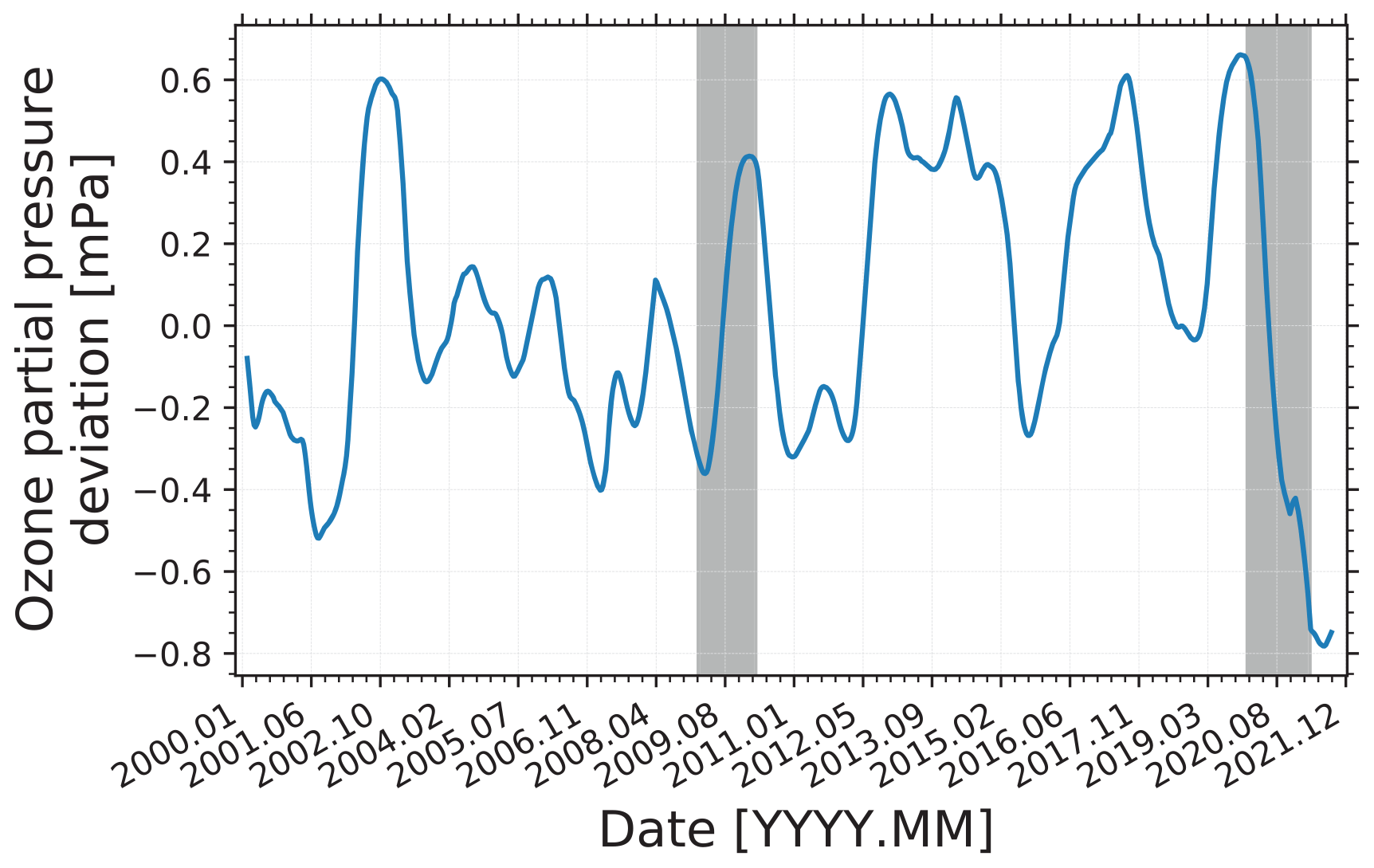
Figure 11Deviation of the monthly mean, vertically averaged (0–35 km height) ozone partial pressure from the respective 2000–2019 long-term monthly mean. Ozone profiles measured regularly (typically one ozonesonde launch per week) at Lauder (New Zealand), the German Antarctic Neumayer Station, and at the South Pole (data from NDACC, 2021) are considered. Gray columns mark two time periods after major Australian fire events in 2009 (Black Saturday) and 2019/2020 (Black Summer).
The ozone hole observed in September–November 2020 was 2 times larger than the Calbuco-related ozone hole. It is thus reasonable to assume that wildfire smoke particles may also be able to contribute to halogen activation and ozone depletion (Yu et al., 2021; Ohneiser et al., 2021; Rieger et al., 2021). However, in contrast to background and volcanic sulfate particles ( droplets), the knowledge about the chemical and microphysical properties of aged wildfire smoke (after many months of traveling around the globe) and about the pathways of the smoke impact on ozone depletion is rather limited. We assume that the aged stratospheric wildfire smoke particles are most likely glassy, show a core shell morphology, and are largely composed of organic material (organic carbon, OC, in the shell) and, to a minor degree, of black carbon (BC, concentrated in the core part; China et al., 2013). Further thin coatings may exist as a result of the condensation of trace gases (injected together with the smoke particles into the stratosphere). The size distribution of the stratospheric smoke particles is well described by an accumulation mode with effective radius of 0.2–0.3 µm (Haarig et al., 2018; Ansmann et al., 2021a; Engelmann et al., 2021; Ohneiser et al., 2021). We hypothesize that these glassy accumulation-mode particles may act as condensation sinks for stratospheric H2O, H2SO4, and HNO3 and may then perturb the stratospheric background aerosol and PSC formation conditions (Ansmann et al., 2022) in a similar way, as demonstrated by Zhu et al. (2018), for volcanic sulfate aerosol.
The injection of wildfire smoke into the UTLS regime with the consequence of severe ozone depletion is a rather new aspect in atmospheric sciences and needs to be explored in future research projects (laboratory studies, airborne in situ observations, and modeling efforts). To initiate and stimulate the required scientific discussion, we showed the smoke and ozone profiles over the North Pole region measured during the MOSAiC expedition in the winter and spring seasons of 2020 (Ohneiser et al., 2021; Voosen, 2021). In this section, we will add new observational data to this discussion. The findings in the Southern Hemisphere are clearer than the High Arctic results.
Figure 11 shows the variations in the ozone partial pressure from the long-term mean. Ozonesonde observations at Lauder (45∘ S, New Zealand, outside of the polar vortex), the Neumayer Station (70.6∘ S, Antarctica, edge of the polar vortex), and at the South Pole (Antarctica, inside the polar vortex) are averaged to determine a robust time series of ozone variations over the last 20 years. Stone et al. (2021) mentioned the pronounced ozone minima in 2015, 2018, and 2020. However, the 2020 minimum is by far the strongest and longest. In 2019 and early 2020, the ozone deviations were positive and then started to decrease continuously towards the record-breaking negative deviations found between August 2020 and March 2021. The gray area in Fig. 11 highlights this remarkable ozone destruction period. The negative standard deviation was twice as large as earlier minima that have been seen since 2002.
The other gray period in Fig. 11 highlights the potential impact of the so-called Black Saturday fires between 7 February–14 March 2009 (Siddaway and Petelina, 2011) on ozone reduction. On Saturday, 7 February 2009 (coinciding with the left boundary of the 2009 gray column), extraordinarily strong fires, in combination with the development of a few pyroCb cloud towers northeast of Melbourne, initiated the injection of wildfire smoke into the stratosphere (de Laat et al., 2012). However, in 2009, a pronounced ozone loss was not observed. Instead, even a moderate increase in the ozone concentration was observed. As discussed by Peterson et al. (2021), the injected smoke amount was an order of magnitude smaller than the injected one observed in December 2019 and January 2020. This 2009 smoke event was obviously too weak to have any influence on ozone depletion.
Figure 12 shows the deviation in the ozone partial pressure (from the 2000–2019 mean value) over the Neumayer research station of the Alfred Wegener Institute (70.6∘ S, 8.3∘ W). The daily smoke layer base and top heights, as measured over Punta Arenas (53.2∘ S, 70.9∘ W), are indicated by gray and black circles, respectively. As mentioned above, data gaps in the lidar time series are caused by cloudy weather or instrumental problems. We assume that the general structures of the smoke layers as measured over Punta Arenas were similar to the ones over the Neumayer Station (about 1900 km further south). In agreement with Fig. 11, large positive ozone deviations from the long-term mean were observed in November and December 2019 before the long-lasting decrease in the ozone partial pressure over about 10 months started. From October 2020 to January 2021, the largest negative ozone deviations were found between 12 and 25 km, well within the Australian smoke layer. As in the case of the strong ozone depletion over the High Arctic (Ohneiser et al., 2021), the polar vortex was unusually strong over Antarctica in July and August 2020 (Copernicus, 2021). The large-scale warming of the southern hemispheric stratosphere (Stocker et al., 2021) as a result of strong absorption of solar radiation by smoke in January to April 2020 may have contributed to the development of a strong vortex over Antarctica in the July–September 2020 by suppressing large-scale wave activity (Tritscher et al., 2021).
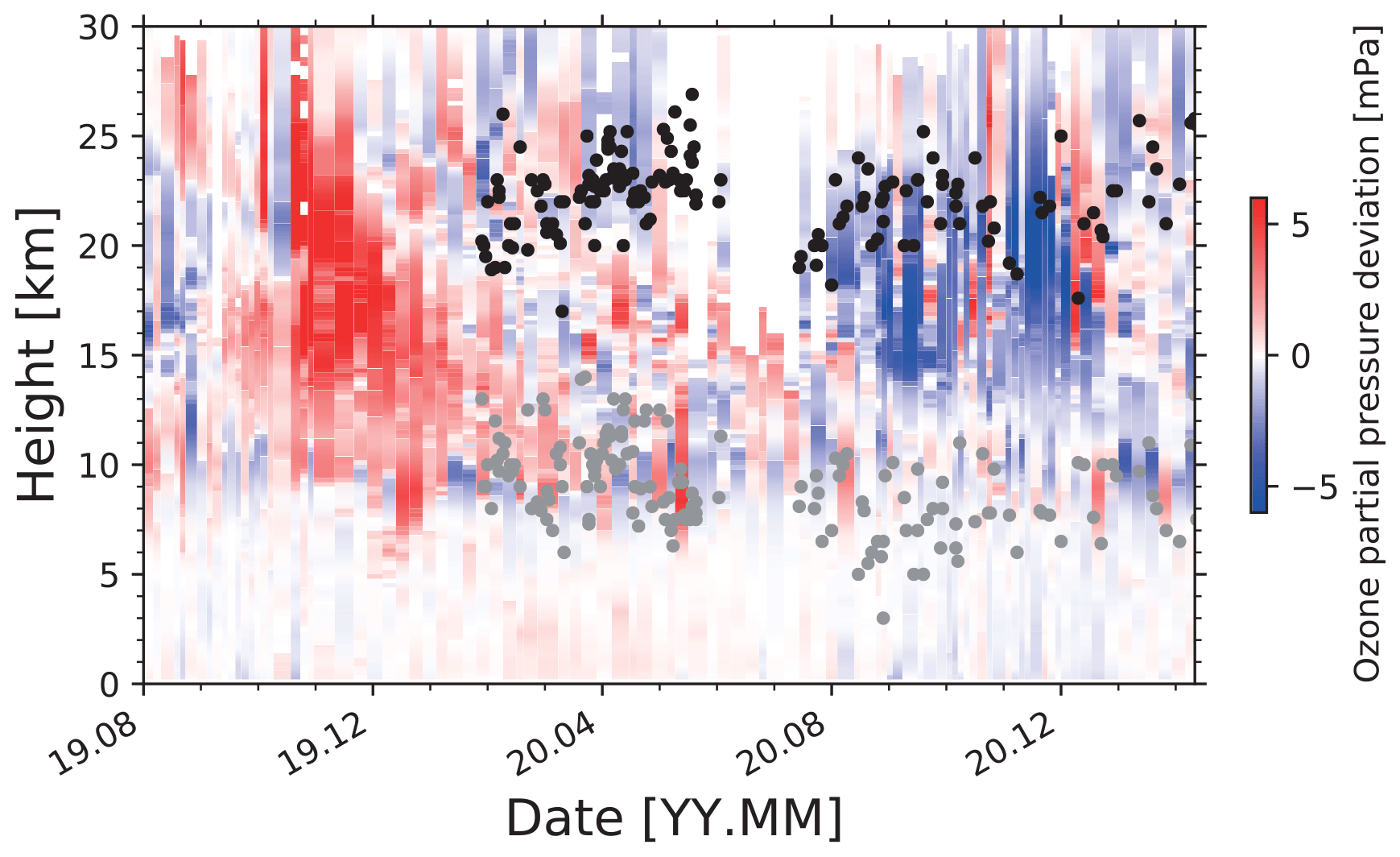
Figure 12Deviation of each individual ozone profile measured at the Neumayer Station (NDACC, 2021) from the respective long-term (2000–2019) monthly mean ozone profile. The base (gray dots) and top heights (black dots) of the Australian smoke layer measured with Polly at Punta Arenas indicate the smoke-polluted height range.
Figure 13 shows height profiles of the September–November 2020 mean particle surface area (SA) concentration together with September–November mean ozone deviations for the long-term mean and the height range with PSCs, as observed with CALIOP. The 2000–2019 mean ozone profile again includes the observations at Lauder (New Zealand), Neumayer Station (Antarctica), and the South Pole station (Antarctica) (NDACC, 2021). The PSC height profile was retrieved by using the CALIPSO V4 classification scheme (CALIPSO, 2021a). All CALIOP data for the Southern Hemisphere during the winter season in 2020 were downloaded, and the number of PSC entries obtained with the CALIPSO V4 classification were available as a function of height. The maximum PSC number was then arbitrarily set to 0.95 in our value range from 0 to 1 in Fig. 13b. Below 13 km height, cirrus clouds are frequently misclassified as PSC; therefore, the PSC height range is shown down to 13 km (in arbitrary units) only. The microphysical properties of the smoke (SA, n50, and n250 in Fig. 13a) were obtained by converting the September–November 2020 mean smoke extinction coefficient profile by using the conversion scheme of Ansmann et al. (2021a). n50 (accumulation mode) and n250 (large particle fraction), considering particles with radius >50 and >250 nm, respectively. The background extinction coefficient profiles in Sakai et al. (2016) were converted into SA, n50, and n250 values as well (dash-dotted gray line in Fig. 13a) by using conversion factors for typical sulfate background accumulation-mode particles with an effective radius around 0.15 µm. Effective radii of aged smoke particles are between 0.2 and 0.3 µm (Ansmann et al., 2021a).
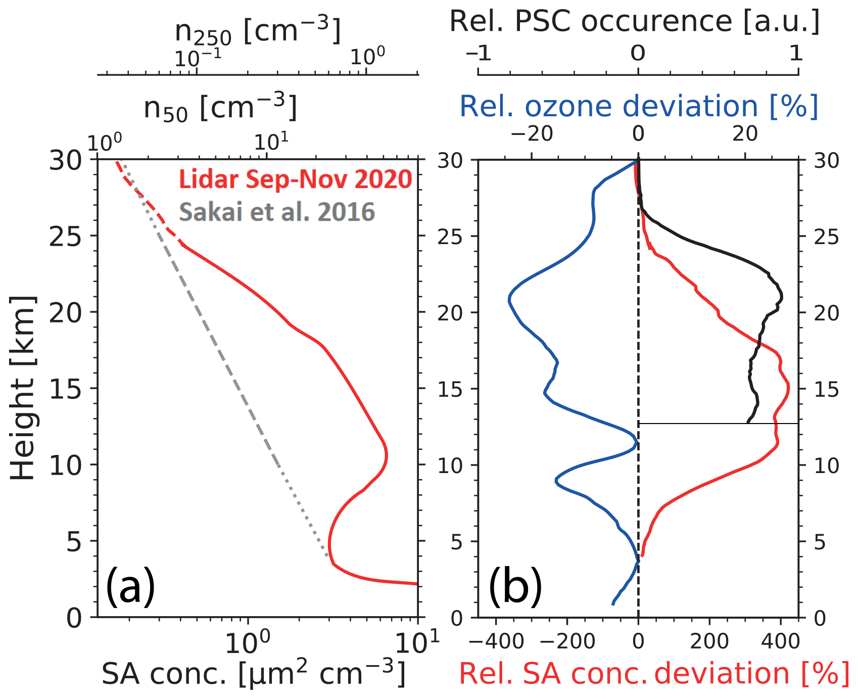
Figure 13(a) Estimated mean profiles of the surface area concentration (SA) and number concentrations n50 and n250 (particles with radius >50 and >250 nm, respectively) for the September–November 2020 time period derived from Polly measurements at Punta Arenas (red). Respective background aerosol estimates are given as a gray dashed line, based on lidar observations at Lauder, New Zealand (Sakai et al., 2016). Dotted line segments indicate extrapolations. (b) Relative increase in the estimated particle surface area concentration (computed by using the gray and red profiles in panel a) and relative deviation of the ozone partial pressure (September–November 2020 mean) from the respective 2000–2019 (September–November) mean ozone value, calculated from the ozonesonde observations at Lauder, New Zealand, the German Antarctic Neumayer Station, and the South Pole station (NDACC, 2021). The height range with PSCs in the Southern Hemisphere north of 81.8∘ S in the winter of 2020 (June–August 2020) above 13 km height (indicated by a horizontal line) obtained from CALIOP observations (CALIPSO, 2021a) is shown in addition. The PSC occurrence frequency per height level is normalized such that the maximum PSC number is 0.95 (further explanations are given in the text).
We observed a clear coincidence between the layer with strongest ozone reduction over the ozonesonde stations (14–25 km height range) and the layer showing an enhanced particle surface area concentration over Punta Arenas (10–24 km height range) and the height range in which CALIOP detected PSCs (mostly over Antarctica at heights from 13–26 km). As can be seen in Fig. 13a, the particle surface area concentration was about a factor 2, 3, and 5 larger at 22, 20, and 15 km height than at unperturbed conditions, respectively. Surface area values of 0.5–5 µm2 cm−3 and particle number concentrations of 25–65 cm−3 (for n50) and 0.15–1 cm−3 or 150–1000 particles per liter (for n250) in the height range from 15–22 km, in which the highest values of ozone reduction were found, clearly indicate a significantly polluted lower stratosphere. The large particle fraction could be regarded as the reservoir of the most favorable ice-nucleating smoke particles available for cirrus and PSC ice formation processes.
According to the dash-dotted line in Fig. 13a, clean background conditions are characterized by values of 2–7 cm−3 for n50 and 0.05–0.2 cm−3 for n250. The surface area concentration of 0.3–1 µm2 cm−3 from 15–22 km height (according to the dashed line) is in good agreement with balloon-borne observations over Laramie (41∘ N), Wyoming, of 0.5–1 µm2 cm−3 at 18–20 km height during volcanic quiescent time in the late 1970s (Hofmann and Solomon, 1989) and in the late 1990s (Deshler et al., 2003).
We assume that, in the PSC height range from 13–26 km, all background particles and most of the -coated smoke particles grew due to HNO3 condensation during PSC events. Compared to PSC-free conditions, the particle surface area concentration and thus the potential for halogen activation strongly increased within the PSCs (Carslaw et al., 1994; Tritscher et al., 2021). The total particle number concentration ntot is typically a factor of 1.3–2 higher than n50 (Deshler et al., 2003). High numbers of smoke particle concentrations (probably ntot>100 cm−3) were found in the PSC height region during the southern hemispheric winter and spring months in 2020 and were probably involved in PSC formation, strong halogen activation, and the resulting record-breaking ozone depletion. More details are given in Ansmann et al. (2022).
We presented a detailed characterization of the geometrical, optical, and microphysical properties of the largest stratospheric wildfire-smoke-related stratospheric perturbation ever observed around the globe. The Australian smoke sensitively affected the radiation budget, dynamical processes, and most probably ozone depletion in the stratosphere of the Southern Hemisphere. We documented this unique and record-breaking wildfire pollution event with two ground-based lidars in southern South America in 2020 and 2021 and found a slow decrease in the smoke perturbation until the end of 2021. Our height-resolved observations can be regarded as representative for mid- and high latitudes in the Southern Hemisphere. The presented observations can be regarded as a benchmark data set for modeling studies and for comparison with active and passive remote sensing products in the framework of quality assurance efforts.
For the second time, a record-breaking ozone hole developed in 2020 in a smoke-polluted stratospheric environment. In the case of the unusually strong Arctic ozone depletion (in March 2020), the impact of smoke on ozone reduction mainly occurred in the lowest part of the stratosphere (10–17 km height range) and thus below the region with strongest ozone depletion (Ohneiser et al., 2021). This time, the height range with pronounced ozone depletion over Antarctica (September–November 2020) fully overlapped with the Australian smoke layer. Strong ozone depletion over Antarctica was even observed in September–November 2021, again at significantly enhanced smoke pollution levels. We will report on this in a follow-up article (Ansmann et al., 2022). As we already hypothesized in Ohneiser et al. (2020), if upcoming studies indicate a link between huge fires (caused by unusually hot temperatures and droughts as a result of climate change), corresponding smoke occurrence in the lower stratosphere, and severe ozone depletion in the Arctic and Antarctica, then the climate change debate will be extended by a new, and until now, not considered important aspect. In other words, climate change will not only change stratospheric chemistry and dynamics by causing stratospheric temperatures to decrease, as associated with a warming troposphere, but also by the injection of new types of particles commonly only present in the troposphere. This is a new parameter that we have to consider in future climate and ozone depletion predictions.
Another research topic is the impact of smoke on cirrus formation in the upper troposphere. Unique data sets for the High Arctic (October 2019 to May 2020) and over southern South America (January 2020 to November 2021) are available for in-depth smoke–cirrus interaction by means of the full active remote sensing equipment available during the MOSAiC and during the DACAPO-PESO long-term campaigns. The tropopause region was permanently polluted over Punta Arenas in 2020 and 2021. A first case study of the smoke impact on cirrus formation was presented by Engelmann et al. (2021), as observed during the MOSAiC expedition.
Polly lidar observations (level 0 data; measured signals) are in the PollyNet database (Polly, 2021). LACROS observations (level 0 data) are stored in the CloudNet database Lacros (2021). All the analysis products are available from TROPOS upon request (info@tropos.de). CORAL data are available from TROPOS and DLR, Oberpfaffenhofen, upon request.
The ozone data are used from the regular ozone launch data at Lauder (New Zealand), Neumayer Station (Antarctica), and the South Pole (Antarctica) and are available at the Network for the Detection of Atmospheric Composition Change (NDACC) website (http://www.ndaccdemo.org/, NDACC, 2021). Besides the continuous lidar measurements, an Aerosol Robotic Network (AERONET) sun photometer was operated (http://aeronet.gsfc.nasa.gov/, AERONET, 2021). Fire and MODIS data are available from the NASA database (https://worldview.earthdata.nasa.gov/, MODIS, 2021a, https://search.earthdata.nasa.gov/search?fp=Terra, MODIS, 2021b, https://giovanni.gsfc.nasa.gov/giovanni/, MODIS, 2021c, https://firms.modaps.eosdis.nasa.gov/download/, FIRMS, 2021). CALIPSO observations were downloaded from the CALIPSO database (https://www-calipso.larc.nasa.gov/tools/data_avail/, CALIPSO, 2021a, https://www-calipso.larc.nasa.gov/products/lidar/browse_images/show_v4_detail.php?s=production&v=V4-10&browse_date=2020-01-27&orbit_time=04-53-59&page=4&granule_name=CAL_LID_L1-Standard-V4-10.2020-01-27T04-53-59ZN.hdf, CALIPSO, 2021b, https://www-calipso.larc.nasa.gov/products/lidar/browse_images/show_v4_detail.php?s=production&v=V4-10&browse_date=2020-02-25&orbit_time=18-21-04&page=3&granule_name=CAL_LID_L1-Standard-V4-10.2020-02-25T18-21-04ZN.hdf, CALIPSO, 2021c). The ozonesonde data can be found at http://www.ndaccdemo.org/ (NDACC, 2021). The radiosonde data are available at http://weather.uwyo.edu/upperair/sounding.html (University of Wyoming, 2021). Sentinel-5 aerosol data are available at https://apps.sentinel-hub.com/eo-browser/?zoom=4&lat=-51.94426&lng=-89.43029&themeId=DEFAULT-THEME&visualizationUrl=https%3A%2F%2Fservices.sentinel-hub.com%2Fogc%2Fwms%2F2c5dc5f7-4c83-40dd-a520-da2c7221568d&datasetId=S5_AER_AI&fromTime=2020-01-26T00%3A00%3A00.000Z&toTime=2020-01-26T19%3A59%3A59.999Z&layerId=AER_AI_354_AND_388_VISUALIZED (Sentinel-5, 2021). GDAS1 (Global Data Assimilation System 1) re-analysis products from the National Weather Service’s National Centers for Environmental Prediction are available at https://www.ready.noaa.gov/gdas1.php (GDAS, 2021).
The paper was written by KO and AA and designed by KO, AA, AC, and DAK. The data analysis was performed by KO, AC, IV and DV, supported by AA, HB, PS, and RE. BK and NK prepared and provided CORAL data and supported the data analysis. BB, CJ, MR, and FZ were involved in the DACAPO-PESO campaign and took care of the station and the continuous measurements. All co-authors contributed to the discussion of the results.
At least one of the (co-)authors is a member of the editorial board of Atmospheric Chemistry and Physics. The peer-review process was guided by an independent editor, and the authors also have no other competing interests to declare.
Publisher’s note: Copernicus Publications remains neutral with regard to jurisdictional claims in published maps and institutional affiliations.
We thank AERONET-Europe for providing an excellent calibration service. AERONET-Europe is part of the ACTRIS project. We thank AERONET, for their continuous efforts to provide high-quality measurements and products. We also thank the CALIPSO team, for their well-organized, easy-to-use internet platforms. The ozonesondes at the NDACC station of the Neumayer station were launched by the Alfred-Wegener-Institut, Helmholtz-Zentrum für Polar- und Meeresforschung (AWI), Bremerhaven, Germany. Measurements at Lauder are funded by NIWA through New Zealand's Ministry of Business, Innovation and Employment (MBIE) Strategic Science Investment Fund (SSIF). NOAA Earth System Research Laboratory, Global Monitoring Division, Boulder, Colorado, USA, is responsible for the South Pole ozonesonde launches. We thank the PIs, Holger Schmithüsen and Peter von der Gathen (Neumayer station), Richard Querel (Lauder station), and Bryan Johnson (South Pole station) and all team members involved in the carefully performed NDACC ozone soundings over decades for the unique high-quality ozone data sets. Monthly average ozone values were produced by the NASA Earth Observations team, based on data provided by the OMI team. We are also grateful to the entire research team (University Magellan, Leipzig University, and TROPOS), for making the 3-year DACAOPO-PESO campaign event become a big success.
The authors acknowledge support through the European Research Infrastructure for the observation of Aerosol, Clouds and Trace Gases ACTRIS (grant nos. 654109 and 739530) from the European Union’s Horizon 2020 Research And Innovation Programme. The field observations at Punta Arenas were partly funded by the German Science Foundation (DFG; project PICNICC; grant no. 408008112). This research has been supported by the U.S. Department of Energy (grant no. DE-SC0021034). The Polarstern Polly data were produced as part of the international Multidisciplinary drifting Observatory for the Study of the Arctic Climate (MOSAiC) with the tag MOSAiC20192020 and Project ID AWI_PS122_00. The development of algorithm for inversion of lidar observations was supported by Russian Science Foundation (project no. 21-17-00114). Publisher’s note: the article processing charges for this publication were not paid by a Russian or Belarusian institution.
This paper was edited by Yves Balkanski and reviewed by two anonymous referees.
Adachi, K., Sedlacek, A. J., Kleinman, L., Springston, S. R., Wang, J., Chand, D., Hubbe, J. M., Shilling, J. E., Onasch, T. B., Kinase, T., Sakata, K., Takahashi, Y., and Buseck, P. R.: Spherical tarball particles form through rapid chemical and physical changes of organic matter in biomass-burning smoke, P. Natl. Acad. Sci. USA, 116, 19336–19341, https://doi.org/10.1073/pnas.1900129116, 2019. a
AERONET: Aerosol Robotic Network aerosol data base, AERONET [data set], http://aeronet.gsfc.nasa.gov/, last access: 3 June 2021. a, b, c
Allen, D. R., Fromm, M. D., Kablick III, G. P., and Nedoluha, G. E.: Smoke with Induced Rotation and Lofting (SWIRL) in the stratosphere, J. Atmos. Sci., 77, 4297–4316, https://doi.org/10.1175/JAS-D-20-0131.1, 2020. a, b, c
Ansmann, A., Wagner, F., Wandinger, U., Mattis, I., Görsdorf, U., Dier, H.-D., and Reichardt, J.: Pinatubo aerosol and stratospheric ozone reduction: Observations over central Europe, J. Geophys. Res.-Atmos., 101, 18775–18785, https://doi.org/10.1029/96JD01373, 1996. a
Ansmann, A., Mattis, I., Wandinger, U., Wagner, F., Reichardt, J., and Deshler, T.: Evolution of the Pinatubo aerosol: Raman lidar observations of particle optical depth, effective radius, mass, and surface area over Central Europe at 53.4∘ N, J. Atmos. Sci., 54, 2630–2641, https://doi.org/10.1175/1520-0469(1997)054<2630:EOTPAR>2.0.CO;2, 1997. a, b
Ansmann, A., Baars, H., Chudnovsky, A., Mattis, I., Veselovskii, I., Haarig, M., Seifert, P., Engelmann, R., and Wandinger, U.: Extreme levels of Canadian wildfire smoke in the stratosphere over central Europe on 21–22 August 2017, Atmos. Chem. Phys., 18, 11831–11845, https://doi.org/10.5194/acp-18-11831-2018, 2018. a, b, c
Ansmann, A., Ohneiser, K., Mamouri, R.-E., Knopf, D. A., Veselovskii, I., Baars, H., Engelmann, R., Foth, A., Jimenez, C., Seifert, P., and Barja, B.: Tropospheric and stratospheric wildfire smoke profiling with lidar: mass, surface area, CCN, and INP retrieval, Atmos. Chem. Phys., 21, 9779–9807, https://doi.org/10.5194/acp-21-9779-2021, 2021a. a, b, c, d, e, f, g, h, i, j, k, l
Ansmann, A., Ohneiser, K., Chudnovsky, A., Baars, H., and Engelmann, R.: CALIPSO aerosol-typing scheme misclassified stratospheric fire smoke: case study from the 2019 Siberian wildfire season, Front. Environ. Sci., 21, 769852, https://doi.org/10.3389/fenvs.2021.769852, 2021b. a, b, c, d
Ansmann, A., Ohneiser, K., Chudnovsky, A., Knopf, D. A., Eloranta, E. W., Villanueva, D., Seifert, P., Radenz, M., Barja, B., Zamorano, F., Jimenez, C., Engelmann, R., Baars, H., Griesche, H., Hofer, J., Althausen, D., and Wandinger, U.: Ozone depletion in the Arctic and Antarctic stratosphere induced by wildfire smoke, Atmos. Chem. Phys. Discuss. [preprint], https://doi.org/10.5194/acp-2022-247, in review, 2022. a, b, c, d, e, f
Baars, H., Ansmann, A., Ohneiser, K., Haarig, M., Engelmann, R., Althausen, D., Hanssen, I., Gausa, M., Pietruczuk, A., Szkop, A., Stachlewska, I. S., Wang, D., Reichardt, J., Skupin, A., Mattis, I., Trickl, T., Vogelmann, H., Navas-Guzmán, F., Haefele, A., Acheson, K., Ruth, A. A., Tatarov, B., Müller, D., Hu, Q., Podvin, T., Goloub, P., Veselovskii, I., Pietras, C., Haeffelin, M., Fréville, P., Sicard, M., Comerón, A., Fernández García, A. J., Molero Menéndez, F., Córdoba-Jabonero, C., Guerrero-Rascado, J. L., Alados-Arboledas, L., Bortoli, D., Costa, M. J., Dionisi, D., Liberti, G. L., Wang, X., Sannino, A., Papagiannopoulos, N., Boselli, A., Mona, L., D'Amico, G., Romano, S., Perrone, M. R., Belegante, L., Nicolae, D., Grigorov, I., Gialitaki, A., Amiridis, V., Soupiona, O., Papayannis, A., Mamouri, R.-E., Nisantzi, A., Heese, B., Hofer, J., Schechner, Y. Y., Wandinger, U., and Pappalardo, G.: The unprecedented 2017–2018 stratospheric smoke event: decay phase and aerosol properties observed with the EARLINET, Atmos. Chem. Phys., 19, 15183–15198, https://doi.org/10.5194/acp-19-15183-2019, 2019. a, b, c, d
Bègue, N., Vignelles, D., Berthet, G., Portafaix, T., Payen, G., Jégou, F., Benchérif, H., Jumelet, J., Vernier, J.-P., Lurton, T., Renard, J.-B., Clarisse, L., Duverger, V., Posny, F., Metzger, J.-M., and Godin-Beekmann, S.: Long-range transport of stratospheric aerosols in the Southern Hemisphere following the 2015 Calbuco eruption, Atmos. Chem. Phys., 17, 15019–15036, https://doi.org/10.5194/acp-17-15019-2017, 2017. a
Boer, M., Resco de Dios, V., and Bradstock, R.: Unprecedented burn area of Australian mega forest fires, Nat. Clim. Change, 10, 171–172, https://doi.org/10.1038/s41558-020-0716-1, 2020. a
CALIPSO: CALIPSO data, NASA [data set], https://www-calipso.larc.nasa.gov/tools/data_avail/, last access: 3 June 2021a. a, b, c
CALIPSO: CALIPSO smoke bubble overflight data, NASA, https://www-calipso.larc.nasa.gov/products/lidar/browse_images/show_v4_detail.php?s=production&v=V4-10&browse_date=2020-01-27&orbit_time=04-53-59&page=4&granule_name=CAL_LID_L1-Standard-V4-10.2020-01-27T04-53-59ZN.hdf, last access: 3 June 2021b. a, b
CALIPSO: CALIPSO smoke bubble overflight data, NASA, https://www-calipso.larc.nasa.gov/products/lidar/browse_images/show_v4_detail.php?s=production&v=V4-10&browse_date=2020-02-25&orbit_time=18-21-04&page=3&granule_name=CAL_LID_L1-Standard-V4-10.2020-02-25T18-21-04ZN.hdf, last access: 3 June 2021c. a
Carslaw, K. S., Luo, B. P., Clegg, S. L., Peter, T., Brimblecombe, P., and Crutzen, P. J.: Stratospheric aerosol growth and HNO3 gas phase depletion from coupled HNO3 and water uptake by liquid particles, Geophys. Res. Lett., 21, 2479–2482, https://doi.org/10.1029/94GL02799, 1994. a, b
China, S., Mazzoleni, C., Gorkowski, K., Aiken, A. C., and Dubey, M. K.: Morphology and mixing state of individual freshly emitted wildfire carbonaceous particles, Nat. Commun., 4, 2122, https://doi.org/10.1038/ncomms3122, 2013. a, b
Copernicus: The 2020 Antarctic Ozone Hole Season, Copernicus Atmosphere Monitoring Service (CAMS), https://atmosphere.copernicus.eu/2020-antarctic-ozone-hole-season, last access: 3 June 2021. a
de Laat, A. T. J., Stein Zweers, D. C., Boers, R., and Tuinder, O. N. E.: A solar escalator: Observational evidence of the self-lifting of smoke and aerosols by absorption of solar radiation in the February 2009 Australian Black Saturday plume, J. Geophys. Res.-Atmos., 117, D04204, https://doi.org/10.1029/2011JD017016, 2012. a
DeLand, M. T., Bhartia, P. K., Kramarova, N., and Chen, Z.: OMPS LP observations of PSC variability during the NH 2019–2020 season, Geophys. Res. Lett., 47, e2020GL090216, https://doi.org/10.1029/2020GL090216, 2020. a
Deshler, T., Hervig, M. E., Hofmann, D. J., Rosen, J. M., and Liley, J. B.: Thirty years of in situ stratospheric aerosol size distribution measurements from Laramie, Wyoming (41∘ N), using balloon-borne instruments, J. Geophys. Res.-Atmos., 108, 4167, https://doi.org/10.1029/2002JD002514, 2003. a, b, c
Dhomse, S. S., Chipperfield, M. P., Feng, W., Hossaini, R., Mann, G. W., and Santee, M. L.: Revisiting the hemispheric asymmetry in midlatitude ozone changes following the Mount Pinatubo eruption: A 3-D model study, Geophys. Res. Lett., 42, 3038–3047, https://doi.org/10.1002/2015GL063052, 2015. a
Engelmann, R., Kanitz, T., Baars, H., Heese, B., Althausen, D., Skupin, A., Wandinger, U., Komppula, M., Stachlewska, I. S., Amiridis, V., Marinou, E., Mattis, I., Linné, H., and Ansmann, A.: The automated multiwavelength Raman polarization and water-vapor lidar PollyXT: the neXT generation, Atmos. Meas. Tech., 9, 1767–1784, https://doi.org/10.5194/amt-9-1767-2016, 2016. a
Engelmann, R., Ansmann, A., Ohneiser, K., Griesche, H., Radenz, M., Hofer, J., Althausen, D., Dahlke, S., Maturilli, M., Veselovskii, I., Jimenez, C., Wiesen, R., Baars, H., Bühl, J., Gebauer, H., Haarig, M., Seifert, P., Wandinger, U., and Macke, A.: Wildfire smoke, Arctic haze, and aerosol effects on mixed-phase and cirrus clouds over the North Pole region during MOSAiC: an introduction, Atmos. Chem. Phys., 21, 13397–13423, https://doi.org/10.5194/acp-21-13397-2021, 2021. a, b, c, d, e
ERA5: ERA5 data, C3S [data set], https://cds.climate.copernicus.eu/cdsapp#!/dataset/reanalysis-era5-pressure-levels?tab=form, last access: 3 June 2021. a
Fernald, F. G.: Analysis of atmospheric lidar observations: some comments, Appl. Opt., 23, 652–653, https://doi.org/10.1364/AO.23.000652, 1984. a, b, c
Fire Information for Resource Management System (FIRMS): FIRMS active fire/hotspot information, NASA FIRMS [data set], https://firms.modaps.eosdis.nasa.gov/download/, last access: 19 November 2021. a, b
Global Data Assimilation System (GDAS): Meteorological database, NOAA [data set], https://www.ready.noaa.gov/gdas1.php, last access: 3 June 2021. a, b
González, R., Toledano, C., Román, R., Mateos, D., Asmi, E., Rodríguez, E., Lau, I., Ferrara, J., D’Elia, R., Antuña-Sánchez, J. C., Cachorro, V., Calle, A., and de Frutos, Á. M.: Characterization of stratospheric smoke particles over the Antarctica by remote sensing instruments, Remote Sensing, 12, 3769, https://doi.org/10.3390/rs12223769, 2020. a
Haarig, M., Ansmann, A., Baars, H., Jimenez, C., Veselovskii, I., Engelmann, R., and Althausen, D.: Depolarization and lidar ratios at 355, 532, and 1064 nm and microphysical properties of aged tropospheric and stratospheric Canadian wildfire smoke, Atmos. Chem. Phys., 18, 11847–11861, https://doi.org/10.5194/acp-18-11847-2018, 2018. a, b, c, d, e, f, g
Haywood, J. M., Jones, A., Clarisse, L., Bourassa, A., Barnes, J., Telford, P., Bellouin, N., Boucher, O., Agnew, P., Clerbaux, C., Coheur, P., Degenstein, D., and Braesicke, P.: Observations of the eruption of the Sarychev volcano and simulations using the HadGEM2 climate model, J. Geophys. Res.-Atmos., 115, D21212, https://doi.org/10.1029/2010JD014447, 2010. a
Heinold, B., Baars, H., Barja, B., Christensen, M., Kubin, A., Ohneiser, K., Schepanski, K., Schutgens, N., Senf, F., Schrödner, R., Villanueva, D., and Tegen, I.: Important role of stratospheric injection height for the distribution and radiative forcing of smoke aerosol from the 2019/2020 Australian wildfires, Atmos. Chem. Phys. Discuss. [preprint], https://doi.org/10.5194/acp-2021-862, in review, 2021. a
Hems, R. F., Schnitzler, E. G., Liu-Kang, C., Cappa, C. D., and Abbatt, J. P.: Aging of atmospheric brown carbon aerosol, ACS Earth and Space Chemistry, 5, 722–748, https://doi.org/10.1021/acsearthspacechem.0c00346, 2021. a
Hirsch, E. and Koren, I.: Record-breaking aerosol levels explained by smoke injection into the stratosphere, Science, 371, 1269–1274, https://doi.org/10.1126/science.abe1415, 2021. a, b, c, d
Hofmann, D. J. and Solomon, S.: Ozone destruction through heterogeneous chemistry following the eruption of El Chichón, J. Geophys. Res.-Atmos., 94, 5029–5041, https://doi.org/10.1029/JD094iD04p05029, 1989. a, b, c
Holben, B. N., Eck, T. F., Slutsker, I., Tanré, D., Buis, J. P., Setzer, A., Vermote, E., Reagan, J. A., Kaufman, Y. J., Nakajima, T., Lavenu, F., Jankowiak, I., and Smirnov, A.: AERONET – A federated instrument network and data archive for aerosol characterization, Remote Sens. Environ., 66, 1–16, https://doi.org/10.1016/S0034-4257(98)00031-5, 1998. a
Inness, A., Chabrillat, S., Flemming, J., Huijnen, V., Langenrock, B., Nicolas, J., Polichtchouk, I., and Razinger, M.: Exceptionally low Arctic stratospheric ozone in spring 2020 as seen in the CAMS reanalysis, J. Geophys. Res.-Atmos., 125, e2020JD033563, https://doi.org/10.1029/2020JD033563, 2020. a
Kablick, G. P., Allen, D. R., Fromm, M. D., and Nedoluha, G. E.: Australian pyroCb smoke generates synoptic-scale stratospheric anticyclones, Geophys. Res. Lett., 47, e2020GL088101, https://doi.org/10.1029/2020GL088101, 2020. a, b, c, d, e, f, g
Kaifler, B. and Kaifler, N.: A Compact Rayleigh Autonomous Lidar (CORAL) for the middle atmosphere, Atmos. Meas. Tech., 14, 1715–1732, https://doi.org/10.5194/amt-14-1715-2021, 2021. a
Kawa, S. R., Newman, P. A., Lait, L. R., Schoeberl, M. R., Stimpfle, R. M., Kohn, D. W., Webster, C. R., May, R. D., Baumgardner, D., Dye, J. E., Wilson, J. C., Chan, K. R., and Loewenstein, M.: Activation of chlorine in sulfate aerosol as inferred from aircraft observations, J. Geophys. Res.-Atmos., 102, 3921–3933, https://doi.org/10.1029/96JD01992, 1997. a
Khaykin, S., Legras, B., Bucci, S., Sellitto, P., Isaksen, L., Tencé, L., Bekki, S., Bourassa, A., Rieger, L., Zawada, D., Jumelet, J., and Godin-Beekmann, S.: The 2019/20 Australian wildfires generated a persistent smoke-charged vortex rising up to 35 km altitude, Nature Communications Earth and Environment, 1, 22, https://doi.org/10.1038/s43247-020-00022-5, 2020. a, b, c, d, e, f, g, h, i
Kirner, O., Müller, R., Ruhnke, R., and Fischer, H.: Contribution of liquid, NAT and ice particles to chlorine activation and ozone depletion in Antarctic winter and spring, Atmos. Chem. Phys., 15, 2019–2030, https://doi.org/10.5194/acp-15-2019-2015, 2015. a
Kloss, C., Berthet, G., Sellitto, P., Ploeger, F., Bucci, S., Khaykin, S., Jégou, F., Taha, G., Thomason, L. W., Barret, B., Le Flochmoen, E., von Hobe, M., Bossolasco, A., Bègue, N., and Legras, B.: Transport of the 2017 Canadian wildfire plume to the tropics via the Asian monsoon circulation, Atmos. Chem. Phys., 19, 13547–13567, https://doi.org/10.5194/acp-19-13547-2019, 2019. a
Kloss, C., Berthet, G., Sellitto, P., Ploeger, F., Taha, G., Tidiga, M., Eremenko, M., Bossolasco, A., Jégou, F., Renard, J.-B., and Legras, B.: Stratospheric aerosol layer perturbation caused by the 2019 Raikoke and Ulawun eruptions and their radiative forcing, Atmos. Chem. Phys., 21, 535–560, https://doi.org/10.5194/acp-21-535-2021, 2021a. a, b, c, d
Kloss, C., Sellitto, P., von Hobe, M., Berthet, G., Smale, D., Krysztofiak, G., Xue, C., Qiu, C., Jégou, F., Ouerghemmi, I., and Legras, B.: Australian fires 2019–2020: tropospheric and stratospheric pollution throughout the whole fire season, Frontiers in Environmental Science, 9, 652024, https://doi.org/10.3389/fenvs.2021.652024, 2021b. a, b, c, d, e, f
Knopf, D. A., Alpert, P. A., and Wang, B.: The role of organic aerosol in atmospheric ice nucleation: a review, ACS Earth and Space Chemistry, 2, 168–202, https://doi.org/10.1021/acsearthspacechem.7b00120, 2018. a
Lacros: LACROS, TROPOS, http://lacros.rsd.tropos.de/, last access: 3 June 2021. a
Lestrelin, H., Legras, B., Podglajen, A., and Salihoglu, M.: Smoke-charged vortices in the stratosphere generated by wildfires and their behaviour in both hemispheres: comparing Australia 2020 to Canada 2017, Atmos. Chem. Phys., 21, 7113–7134, https://doi.org/10.5194/acp-21-7113-2021, 2021. a, b, c
Magaritz-Ronen, L. and Raveh-Rubin, S.: Wildfire smoke highlights troposphere-to-stratosphere pathway, Geophys. Res. Lett., 48, e2021GL095848, https://doi.org/10.1029/2021GL095848, 2021. a
Maturilli, M., Holdridge, D. J., Dahlke, S., Graeser, J., Sommerfeld, A., Jaiser, R., Deckelmann, H., and Schulz, A.: Initial radiosonde data from 2019-10 to 2020-09 during project MOSAiC. Alfred Wegener Institute, Helmholtz Centre for Polar and Marine Research, Bremerhaven, PANGAEA [data set], https://doi.org/10.1594/PANGAEA.928656, 2021.
McCormick, M., Thomason, L., and Trepte, C.: Atmospheric effects of the Mt Pinatubo eruption, Nature, 373, 399–404, https://doi.org/10.1038/373399a0, 1995. a
MODIS: MODIS daily reflectance images from NASA Worldview, NASA, https://worldview.earthdata.nasa.gov/, last access: 19 November 2021a. a, b, c, d
MODIS: MODIS daily images via Earthdata Search, NASA, https://search.earthdata.nasa.gov/search?fp=Terra, last access: 19 November 2021b. a, b, c, d
MODIS: MODIS geophysical parameters visualized via the Giovanni application, NASA, https://giovanni.gsfc.nasa.gov/giovanni/, last access: 19 November 2021c. a, b, c, d, e, f, g
Müller, D., Mattis, I., Wandinger, U., Ansmann, A., Althausen, D., and Stohl, A.: Raman lidar observations of aged Siberian and Canadian forest fire smoke in the free troposphere over Germany in 2003: Microphysical particle characterization, J. Geophys. Res.-Atmos., 110, D17201, https://doi.org/10.1029/2004JD005756, 2005. a
Nagai, T., Liley, B., Sakai, T., Shibata, T., and Uchino, O.: Post-Pinatubo evolution and subsequent trend of the stratospheric aerosol layer observed by mid-latitude lidars in both hemispheres, SOLA, 6, 69–72, https://doi.org/10.2151/sola.2010-018, 2010. a
NDACC: Network for the Detection of Atmospheric Composition Change, ozonesonde profiles, NDACC, http://www.ndaccdemo.org/, last access: 3 June 2021. a, b, c, d, e, f, g
Ohneiser, K., Ansmann, A., Baars, H., Seifert, P., Barja, B., Jimenez, C., Radenz, M., Teisseire, A., Floutsi, A., Haarig, M., Foth, A., Chudnovsky, A., Engelmann, R., Zamorano, F., Bühl, J., and Wandinger, U.: Smoke of extreme Australian bushfires observed in the stratosphere over Punta Arenas, Chile, in January 2020: optical thickness, lidar ratios, and depolarization ratios at 355 and 532 nm, Atmos. Chem. Phys., 20, 8003–8015, https://doi.org/10.5194/acp-20-8003-2020, 2020. a, b, c, d, e, f, g, h, i, j, k, l, m
Ohneiser, K., Ansmann, A., Chudnovsky, A., Engelmann, R., Ritter, C., Veselovskii, I., Baars, H., Gebauer, H., Griesche, H., Radenz, M., Hofer, J., Althausen, D., Dahlke, S., and Maturilli, M.: The unexpected smoke layer in the High Arctic winter stratosphere during MOSAiC 2019–2020 , Atmos. Chem. Phys., 21, 15783–15808, https://doi.org/10.5194/acp-21-15783-2021, 2021. a, b, c, d, e, f, g, h, i, j, k, l, m, n, o, p, q
Peterson, D. A., Campbell, J. R., Hyer, E. J., Fromm, M. D., Kablick, G. P., Cossuth, J. H., and DeLand, M. T.: Wildfire-driven thunderstorms cause a volcano-like stratospheric injection of smoke, npj Clim. Atmos. Sci., 1, 30, https://doi.org/10.1038/s41612-018-0039-3, 2018. a, b, c, d
Peterson, D. A., Fromm, M. D., McRae, R. H. D., Campbell, J. R., Hyer, E. J., Taha, G., Camacho, C. P., Kablick, G. P., Schmidt, C. C., and DeLand, M. T.: Australia’s Black Summer pyrocumulonimbus super outbreak reveals potential for increasingly extreme stratospheric smoke events, npj Clim. Atmos. Sci., 4, 38, https://doi.org/10.1038/s41612-021-00192-9, 2021. a, b, c, d, e, f, g
Polly: PollyNET lidar data base, PollyNET, http://polly.tropos.de/, last access: 3 June 2021. a
Portmann, R. W., Solomon, S., Garcia, R. R., Thomason, L. W., Poole, L. R., and McCormick, M. P.: Role of aerosol variations in anthropogenic ozone depletion in the polar regions, J. Geophys. Res.-Atmos., 101, 22991–23006, https://doi.org/10.1029/96JD02608, 1996. a
Pumphrey, H. C., Schwartz, M. J., Santee, M. L., Kablick III, G. P., Fromm, M. D., and Livesey, N. J.: Microwave Limb Sounder (MLS) observations of biomass burning products in the stratosphere from Canadian forest fires in August 2017, Atmos. Chem. Phys., 21, 16645–16659, https://doi.org/10.5194/acp-21-16645-2021, 2021. a
Radenz, M., Bühl, J., Seifert, P., Baars, H., Engelmann, R., Barja González, B., Mamouri, R.-E., Zamorano, F., and Ansmann, A.: Hemispheric contrasts in ice formation in stratiform mixed-phase clouds: disentangling the role of aerosol and dynamics with ground-based remote sensing, Atmos. Chem. Phys., 21, 17969–17994, https://doi.org/10.5194/acp-21-17969-2021, 2021. a
Rapp, M., Kaifler, B., Dörnbrack, A., Gisinger, S., Mixa, T., Reichert, R., Kaifler, N., Knobloch, S., Eckert, R., Wildmann, N., Giez, A., Krasauskas, L., Preusse, P., Geldenhuys, M., Riese, M., Woiwode, W., Friedl-Vallon, F., Sinnhuber, B., Torre, A. d. l., Alexander, P., Hormaechea, J. L., Janches, D., Garhammer, M., Chau, J. L., Conte, J. F., Hoor, P., and Engel, A.: SOUTHTRAC-GW: An airborne field campaign to explore gravity wave dynamics at the world's strongest hotspot, B. Am. Meteorol. Soc., 102, E871–E893, https://doi.org/10.1175/BAMS-D-20-0034.1, 2021. a
Rieger, L. A., Randel, W. J., Bourassa, A. E., and Solomon, S.: Stratospheric Temperature and Ozone Anomalies Associated With the 2020 Australian New Year Fires, Geophys. Res. Lett., 48, e2021GL095898, https://doi.org/10.1029/2021GL095898, 2021. a
Rodriguez, B., Lareau, N. P., Kingsmill, D. E., and Clements, C. B.: Extreme pyroconvective updrafts during a megafire, Geophys. Res. Lett., 47, e2020GL089001, https://doi.org/10.1029/2020GL089001, 2020. a
Rosenfeld, D., Fromm, M., Trentmann, J., Luderer, G., Andreae, M. O., and Servranckx, R.: The Chisholm firestorm: observed microstructure, precipitation and lightning activity of a pyro-cumulonimbus, Atmos. Chem. Phys., 7, 645–659, https://doi.org/10.5194/acp-7-645-2007, 2007. a
Sakai, T., Uchino, O., Nagai, T., Liley, B., Morino, I., and Fujimoto, T.: Long-term variation of stratospheric aerosols observed with lidars over Tsukuba, Japan, from 1982 and Lauder, New Zealand, from 1992 to 2015, J. Geophys. Res.-Atmos., 121, 10283–10293, https://doi.org/10.1002/2016JD025132, 2016. a, b, c, d, e, f, g, h, i
Sedlacek III, A. J., Buseck, P. R., Adachi, K., Onasch, T. B., Springston, S. R., and Kleinman, L.: Formation and evolution of tar balls from northwestern US wildfires, Atmos. Chem. Phys., 18, 11289–11301, https://doi.org/10.5194/acp-18-11289-2018, 2018. a
Sekiya, T., Sudo, K., and Nagai, T.: Evolution of stratospheric sulfate aerosol from the 1991 Pinatubo eruption: Roles of aerosol microphysical processes, J. Geophys. Res.-Atmos., 121, 2911–2938, https://doi.org/10.1002/2015JD024313, 2016. a, b
Sentinel-5: Sentinel-5 Aerosol index 340–380 nm, EO Browser, https://apps.sentinel-hub.com/eo-browser/?zoom=4&lat=-51.94426&lng=-89.43029&themeId=DEFAULT-THEME&visualizationUrl=https%3A%2F%2Fservices.sentinel-hub.com%2Fogc%2Fwms%2F2c5dc5f7-4c83-40dd-a520-da2c7221568d&datasetId=S5_AER_AI&fromTime=2020-01-26T00%3A00%3A00.000Z&toTime=2020-01-26T19%3A59%3A59.999Z&layerId=AER_AI_354_AND_388_VISUALIZED, last access: 3 June 2021. a, b, c
Siddaway, J. M. and Petelina, S. V.: Transport and evolution of the 2009 Australian Black Saturday bushfire smoke in the lower stratosphere observed by OSIRIS on Odin, J. Geophys. Res.-Atmos., 116, D06203, https://doi.org/10.1029/2010JD015162, 2011. a
Solomon, S., Daniel, J. S., Neely, R. R., Vernier, J.-P., Dutton, E. G., and Thomason, L. W.: The persistently variable “background” stratospheric aerosol layer and global climate change, Science, 333, 866–870, https://doi.org/10.1126/science.1206027, 2011. a
Stenchikov, G., Ukhov, A., Osipov, S., Ahmadov, R., Grell, G., Cady-Pereira, K., Mlawer, E., and Iacono, M.: How does a Pinatubo-size volcanic cloud reach the middle stratosphere?, J. Geophys. Res.-Atmos., 126, e2020JD033829, https://doi.org/10.1029/2020JD033829, 2021. a
Stocker, M., Ladstädter, F., and Steiner, A.: Observing the climate impact of large wildfires on stratospheric temperature, Nature Scientific Reports, 11, 22994, https://doi.org/10.1038/s41598-021-02335-7, 2021. a, b
Stone, K. A., Solomon, S., Kinnison, D. E., and Mills, M. J.: On recent large Antarctic ozone holes and ozone recovery metrics, Geophys. Res. Lett., 48, e2021GL095232, https://doi.org/10.1029/2021GL095232, 2021. a, b, c, d
Tencé, F., Jumelet, J., Sarkissian, A., Bekki, S., and Khaykin, S.: Optical properties of smoke particules from Australian 2019-20 wildfires derived from lidar measurements at the French Antarctic station Dumont d’Urville, EGU General Assembly 2021, online, 19–30 Apr 2021, EGU21-12466, https://doi.org/10.5194/egusphere-egu21-12466, 2021. a, b
Tritscher, I., Pitts, M. C., Poole, L. R., Alexander, S. P., Cairo, F., Chipperfield, M. P., Grooß, J.-U., Höpfner, M., Lambert, A., Luo, B., Molleker, S., Orr, A., Salawitch, R., Snels, M., Spang, R., Woiwode, W., and Peter, T.: Polar stratospheric clouds: satellite observations, processes, and role in ozone depletion, Rev. Geophys., 59, e2020RG000702, https://doi.org/10.1029/2020RG000702, 2021. a, b
University of Wyoming: Radiosonde data, daily launches, University of Wyoming [data set], http://weather.uwyo.edu/upperair/sounding.html, last access: 3 June 2021. a, b
Veselovskii, I., Kolgotin, A., Griaznov, V., Müller, D., Wandinger, U., and Whiteman, D. N.: Inversion with regularization for the retrieval of tropospheric aerosol parameters from multiwavelength lidar sounding, Appl. Opt., 41, 3685–3699, https://doi.org/10.1364/AO.41.003685, 2002. a
Voosen, P.: High-flying wildfire smoke poses potential threat to ozone layer, Science, 374, 921–922, https://doi.org/10.1126/science.acx9655, 2021. a, b
Wandinger, U., Müller, D., Böckmann, C., Althausen, D., Matthias, V., Bösenberg, J., Weiß, V., Fiebig, M., Wendisch, M., Stohl, A., and Ansmann, A.: Optical and microphysical characterization of biomass- burning and industrial-pollution aerosols from- multiwavelength lidar and aircraft measurements, J. Geophys. Res.-Atmos., 107, 7–21, https://doi.org/10.1029/2000JD000202, 2002. a
Wegner, T., Grooß, J.-U., von Hobe, M., Stroh, F., Sumińska-Ebersoldt, O., Volk, C. M., Hösen, E., Mitev, V., Shur, G., and Müller, R.: Heterogeneous chlorine activation on stratospheric aerosols and clouds in the Arctic polar vortex, Atmos. Chem. Phys., 12, 11095–11106, https://doi.org/10.5194/acp-12-11095-2012, 2012. a
Wilka, C., Solomon, S., Kinnison, D., and Tarasick, D.: An Arctic ozone hole in 2020 if not for the Montreal Protocol, Atmos. Chem. Phys., 21, 15771–15781, https://doi.org/10.5194/acp-21-15771-2021, 2021. a
Winker, D. M., Vaughan, M. A., Omar, A., Hu, Y., Powell, K. A., Liu, Z., Hunt, W. H., and Young, S. A.: Overview of the CALIPSO Mission and CALIOP Data Processing Algorithms, J. Atmos. Ocean. Tech., 26, 2310–2323, https://doi.org/10.1175/2009JTECHA1281.1, 2009. a
Wohltmann, I., Gathen, P., Lehmann, R., Maturilli, M., Deckelmann, H., Manney, G. L., Davies, J., Tarasick, D., Jepsen, N., Kivi, R., Lyall, N., and Rex, M.: Near‐complete local reduction of Arctic stratospheric ozone by severe chemical loss in spring 2020, Geophys. Res. Lett., 47, e2020GL089547, https://doi.org/10.1029/2020GL089547, 2020. a
Yu, P., Davis, S. M., Toon, O. B., Portmann, R. W., Bardeen, C. G., Barnes, J. E., Telg, H., Maloney, C., and Rosenlof, K. H.: Persistent stratospheric warming due to 2019–2020 Australian wildfire smoke, Geophys. Res. Lett., 48, e2021GL092609, https://doi.org/10.1029/2021GL092609, 2021. a
Yuan, Q., Xu, J., Liu, L., Zhang, A., Liu, Y., Zhang, J., Wan, X., Li, M., Qin, K., Cong, Z., Wang, Y., Kang, S., Shi, Z., Pósfai, M., and Li, W.: Evidence for large amounts of brown carbonaceous tarballs in the Himalayan atmosphere, Environ. Sci. Tech. Let., 8, 16–23, https://doi.org/10.1021/acs.estlett.0c00735, 2021. a
Zhu, Y., Toon, O. B., Kinnison, D., Harvey, V. L., Mills, M. J., Bardeen, C. G., Pitts, M., Bègue, N., Renard, J.-B., Berthet, G., and Jégou, F.: Stratospheric aerosols, polar stratospheric clouds, and polar ozone depletion after the Mount Calbuco eruption in 2015, J. Geophys. Res.-Atmos., 123, 12308–12331, https://doi.org/10.1029/2018JD028974, 2018. a, b
- Abstract
- Introduction
- Lidar and photometer observations, data analysis, and auxiliary meteorological data
- Results
- Smoke impact on ozone depletion
- Conclusion and outlook
- Data availability
- Author contributions
- Competing interests
- Disclaimer
- Acknowledgements
- Financial support
- Review statement
- References