the Creative Commons Attribution 4.0 License.
the Creative Commons Attribution 4.0 License.
 | 07 Jun 2022
Eurodelta multi-model simulated and observed particulate matter trends in Europe in the period of 1990–2010
Wenche Aas
Augustin Colette
Camilla Andersson
Bertrand Bessagnet
Giancarlo Ciarelli
Florian Couvidat
Kees Cuvelier
Astrid Manders
Kathleen Mar
Mihaela Mircea
Noelia Otero
Maria-Teresa Pay
Valentin Raffort
Yelva Roustan
Mark R. Theobald
Marta G. Vivanco
Hilde Fagerli
Peter Wind
Gino Briganti
Andrea Cappelletti
Massimo D'Isidoro
Mario Adani
The Eurodelta-Trends (EDT) multi-model experiment, aimed at assessing the efficiency of emission mitigation measures in improving air quality in Europe during 1990–2010, was designed to answer a series of questions regarding European pollution trends; i.e. were there significant trends detected by observations? Do the models manage to reproduce observed trends? How close is the agreement between the models and how large are the deviations from observations? In this paper, we address these issues with respect to particulate matter (PM) pollution. An in-depth trend analysis has been performed for PM10 and PM2.5 for the period of 2000–2010, based on results from six chemical transport models and observational data from the EMEP (Cooperative Programme for Monitoring and Evaluation of the Long-range Transmission of Air Pollutants in Europe) monitoring network. Given harmonization of set-up and main input data, the differences in model results should mainly result from differences in the process formulations within the models themselves, and the spread in the model-simulated trends could be regarded as an indicator for modelling uncertainty.
The model ensemble simulations indicate overall decreasing trends in PM10 and PM2.5 from 2000 to 2010, with the total reductions of annual mean concentrations by between 2 and 5 (7 for PM10) µg m−3 (or between 10 % and 30 %) across most of Europe (by 0.5–2 µg m−3 in Fennoscandia, the north-west of Russia and eastern Europe) during the studied period. Compared to PM2.5, relative PM10 trends are weaker due to large inter-annual variability of natural coarse PM within the former. The changes in the concentrations of PM individual components are in general consistent with emission reductions. There is reasonable agreement in PM trends estimated by the individual models, with the inter-model variability below 30 %–40 % over most of Europe, increasing to 50 %–60 % in the northern and eastern parts of the EDT domain.
Averaged over measurement sites (26 for PM10 and 13 for PM2.5), the mean ensemble-simulated trends are −0.24 and −0.22 µg m−3 yr−1 for PM10 and PM2.5, which are somewhat weaker than the observed trends of −0.35 and −0.40 µg m−3 yr−1 respectively, partly due to model underestimation of PM concentrations. The correspondence is better in relative PM10 and PM2.5 trends, which are −1.7 % yr−1 and −2.0 % yr−1 from the model ensemble and −2.1 % yr−1 and −2.9 % yr−1 from the observations respectively. The observations identify significant trends (at the 95 % confidence level) for PM10 at 56 % of the sites and for PM2.5 at 36 % of the sites, which is somewhat less that the fractions of significant modelled trends. Further, we find somewhat smaller spatial variability of modelled PM trends with respect to the observed ones across Europe and also within individual countries.
The strongest decreasing PM trends and the largest number of sites with significant trends are found for the summer season, according to both the model ensemble and observations. The winter PM trends are very weak and mostly insignificant. Important reasons for that are the very modest reductions and even increases in the emissions of primary PM from residential heating in winter. It should be kept in mind that all findings regarding modelled versus observed PM trends are limited to the regions where the sites are located.
The analysis reveals considerable variability of the role of the individual aerosols in PM10 trends across European countries. The multi-model simulations, supported by available observations, point to decreases in concentrations playing an overall dominant role. Also, we see relatively large contributions of the trends of and to PM10 decreasing trends in Germany, Denmark, Poland and the Po Valley, while the reductions of primary PM emissions appear to be a dominant factor in bringing down PM10 in France, Norway, Portugal, Greece and parts of the UK and Russia. Further discussions are given with respect to emission uncertainties (including the implications of not accounting for forest fires and natural mineral dust by some of the models) and the effect of inter-annual meteorological variability on the trend analysis.
- Article
(23422 KB) - Full-text XML
- BibTeX
- EndNote


The Convention on Long-range Transboundary Air Pollution (LRTAP), signed in 1979, addresses some of the major environmental problems of the United Nations Economic Commission for Europe (UNECE) region through scientific collaboration and policy negotiation (UNECE, 2004). Parties develop policies and strategies to combat the release of pollutants in the atmosphere through exchanges of information, consultation, research and monitoring. During the 1980s, 1990s and 2000s, the concentrations of particulate matter (PM) were decreasing due to the decrease in secondary inorganic aerosols (SIA) as a result of the reductions of the emissions of their gaseous precursors in order to address the acidification and eutrophication problems (Fagerli and Aas, 2008; Aas et al., 2019), mainly of SOx due to the first and second Sulphur Protocols and also NOx and NH3, in line with the 1999 Gothenburg Protocol to Abate Acidification, Eutrophication and Ground-level Ozone (UNECE, 2004). The emissions of primary PM were not then regulated but were still decreasing as a side effect of the reductions of gaseous pollutants. At the end of the 1990s, the issue of adverse effects of particulate pollution on human health came into focus, and in 2012, emissions of primary PM2.5 were included in the revised Gothenburg Protocol, stating that fine particulate matter is “the pollutant whose ambient air concentrations notoriously exceed air quality standards throughout Europe”.
The Eurodelta-Trends (EDT) multi-model experiment, involving eight chemical transport models (CTMs), has been designed in order to better understand the evolution of air pollution and its drivers since the early 1990s. The main objective of the experiment is to assess the efficiency of air pollutant emission mitigation measures in improving regional-scale air quality in Europe. The multi-model trend analysis is a contribution to the assessment of the evolution of air pollution in the Cooperative Programme for Monitoring and Evaluation of the Long-range Transmission of Air Pollutants in Europe (EMEP) region over the 1990–2012 period coordinated by the Task Force on Monitoring and Modelling (TFMM) of EMEP. The synthesis of the observational and modelling evidence of atmospheric composition and deposition change in response to actions taken to control emissions was given in Colette et al. (2016).
A number of studies of European (and global) PM trends for the 1990s and 2000s have been performed and published recently. Some studies analysed observed PM trends (e.g. Guerreiro et al., 2014; Barmpadimos et al., 2012; Cusack et al., 2012; EEA, 2009; Crippa et al., 2016), including those derived from remote sensing observations (Van Donkelaar et al., 2015), whereas a limited number of analyses also included model simulations (e.g. Colette et al., 2011; Mortier et al., 2020; Colette et al., 2021; Myhre et al., 2017). A rather large spread of observed and modelled PM trends, both decreasing and increasing, has been reported for the period between 1998–2002 and 2008–2014. In those studies, the set-up of model runs was only partly harmonized; i.e. the models in the same study used the same emissions but otherwise different meteorology, grid resolution, etc. Analysis of EMEP-observed 2002–2012 trends, also performed under TFMM coordination by Colette et al. (2016), reported the median trends of −0.35 µg m−3 yr−1 PM10 and −0.29 for PM2.5, resulting in the reduction over the period by −29 $ and −31 % respectively, with 95 % probability. As we discuss in this paper, being overall consistent with the earlier trend assessments, the results presented here are believed to be more robust as they rely on a multi-modelling approach.
The main science and policy questions addressed by the EDT modelling experiment are formulated in Colette et al. (2017a), in which the design and technical specifics of the modelling exercise are also described in detail. The studied period covered a 21-year time span, from 1990 through 2010, and in total eight regional CTMs participated. In this paper, we present the results of trend study with respect to particulate matter (PM) pollution in Europe. An in-depth trend analysis for PM10 and PM2.5 has been performed for the period of 2000–2010, based on multi-model simulations and EMEP monitoring data. The shorter period for PM trend study than the 1990–2010 EDT period was chosen due to the lack of appropriate PM10 and PM2.5 observations prior to 2000. Not all of the eight EDT models had resources to perform all simulations (Sect. 2.1, and therefore trend analyses presented in this work are based on the results from six of the models. Also, multi-model simulated PM trends during the whole 1990–2010 period are briefly discussed here. The strength of the presented assessment is that the model-ensemble-simulated PM trends represent more a robust estimate as compared to either of the individual models, while the multi-model simulations allowed us to investigate the variability of modelled results obtained under this controlled set-up. Finally, the model simulations allow interpretation of PM trends in terms of the trends in the individual aerosols. This is a valuable contribution to better understanding the correspondence between emission changes and PM concentration levels across Europe, given the lack of observational data on PM chemical composition.
The paper is structured as follows. Section 2 describes the methods used, including brief information on the model and run set-up, observations and trend calculations. Section 3 summarizes model evaluation with respect to PM. Section 4 presents emission trends. Section 5 is dedicated to PM 2000–2010 trend analysis for the whole of Europe and for the set of measurement sites and discusses PM seasonal trends and the relative contribution of PM components. In Sect. 6 we show modelled PM trends for the 1990–2010 period. Further discussion of the result is given in Sect. 7 (including emission uncertainties and the effect of meteorological variability), and finally the main outcomes and findings can be found in Sect. 8.
2.1 Model and run set-up
The trend analysis is based on the results from six of the EDT models, namely the ones which provided a complete series of 2000–2010 simulations. Those models are CHIMERE (CHIM), EMEP MSC-W (EMEP), LOTOS-EUROS (LOTO), MATCH, MINNI and Polair3D (POLR). These models, with the exception of POLR, also performed simulations for the 1990–1999 period. A comprehensive description of the models that participated in the Eurodelta-Trends experiment, the simulation set-up, the input data and the overview of the computations performed are given in Colette et al. (2017a).
Briefly, the set-up and input data for the EDT simulations were harmonized as far as possible. The models performed the simulations on the same grid with a resolution of in latitude–longitude coordinates. The simulations were driven by the same meteorological input from hindcast simulations of the CORDEX project (Jacob et al., 2014; Stegehuis et al., 2015) using the WRF (Weather Research and Forecast) model (Skamarock et al., 2005) at resolution and using boundary conditions from ERA-Interim reanalysis (Dee et al., 2011). The exceptions were LOTO and MATCH, which used ERA-Interim reanalysis downscaled respectively by RACMO2 (Van Meijgaard et al., 2012) and HIRLAM (Dahlgren et al., 2016).
Furthermore, the models used the same gridded anthropogenic emissions of SO2, NOx, NH3, non-methane volatile organic compounds (NMVOCs), CO, PM10 and PM2.5 (Terrenoire et al., 2015; Bessagnet et al., 2016). The national emissions were based on the ECLIPSE_V5 dataset, constructed by the Greenhouse Gases and Air pollution INteraction and Synergies (GAINS) model (Amann et al., 2011; Amann, 2012; Klimont et al., 2016, 2017) and provided in SNAP (Selected Nomenclature for reporting of Air Pollutants) sectors. Spatial distribution of the national sectoral emissions was performed by INERIS applying auxiliary information which included road maps (for SNAP sector 7), shipping routes (for SNAP 8) and population density (for SNAP 2), the European Pollutant Release and Transfer Register (for SNAP 1, 3, and 4), the TNO-MACC inventory for NH3 emissions, as well as bottom-up emission inventories for the UK and France (see details in Colette et al., 2017a, and references therein). Time changes in the spatial distribution were accounted for only for industrial emissions. Vertical distribution and temporal profiles for the emissions used in the model simulations were those used in the EMEP model standard set-up (Simpson et al., 2012). The ECLIPSE_V5 emissions were available for the years 1990, 1995, 2000, 2005 and 2010, while for the intermediate years the emissions were derived through linear interpolations (Colette et al., 2017a). For temporal distribution of ECLIPSE annual emissions, the models applied the same monthly and hourly profiles based on Denier van der Gon et al. (2011); they also used the same static vertical profiles for the emissions, based on Bieser et al. (2011), applied per SNAP activity sector (none of the models included explicit plume rise simulations). Regarding chemical speciation of PM10 and PM2.5, the models were allowed to use their own preferred factors to split PM emission into elemental and primary organic carbon (e.g. based on Kuenen et al., 2014, or as in Simpson et al., 2012; see Table A in the Appendix).
At a rather late stage of the experiment, an error was detected in the emissions of primary particulate matter from international shipping and also from Russia and northern Africa for the period 1991–1999. Since this error was identified late in the analysis process, it was not possible to re-run the simulations with corrected emissions. The additional analysis of the impact of this error carried out with the CHIMERE model showed that these errors are relatively small compared to the overall uncertainty of the model estimates and the uncertainty of the observations (see more details in Theobald et al., 2019). Nevertheless, the main focus of this paper is on the analysis of PM trends in the course of the 2000s, i.e. the period for which model results were not affected by the emission error.
Natural emissions of biogenic VOCs, soil NOx, sea salt and mineral dust were calculated or prescribed within the models individually. Online computations of windblown dust from erodible soils were performed by EMEP, LOTO and MINNI, whereas the other models included solely mineral dust from boundary conditions. Emissions from forest fires and volcanoes were not included in the EDT simulations, as the main research focus was to investigate whether the models could reproduce the trends caused by anthropogenic emission changes and changes in meteorology (see discussions on possible implications of not accounting for forest fires and volcanoes emissions in Sect. 7). Finally, the common boundary conditions provided by the EMEP group were based mainly on a climatology of observational data (Simpson et al., 2012). Given harmonization of set-up and main input data (with a few exceptions), the differences in model results should mainly result from differences in the process formulations within the models themselves.
2.2 Observations
The observations collected at the EMEP monitoring network are annually reported to the Chemical Coordinating Centre of EMEP (Tørseth et al., 2012). All submitted observational data, after routine quality and consistency control, are available in EBAS (http://ebas.nilu.no, last access: 19 January 2022). At most of the sites, 24-hourly samples were taken on a daily basis (see Table A). Most of the sites used a gravimetric method for both size fractions, though some used monitors. The same methods are used during the whole period. Details about site locations and applied methods are found in Table A.
As documented in Colette et al. (2016), the selection criteria for sites included in the trend analysis were that (i) the data capture should be at least 75 % for a specific year to be counted and (ii) the number of these counted years should be at least 75 % of the total number of years in the period and have undergone visual screening tests. The datasets used in this work include yearly measurements of observed trends from respectively 26 and 13 sites of PM10 and PM2.5 for the period 2000–2010 (Table A and Fig. 5a).
Among those “trend sites”, PM10 observations are available for all 11 years of the 2000–2010 period at 16 sites and at 4 sites for PM2.5 (Table A). The reason for gap years is either that PM was not measured in that year or that the criterion of 75 % for data coverage was not satisfied. For most of the sites with incomplete data series, 2000 is a gap year, as PM monitoring was not started before 2001 at those sites. The other gap years are 2009 at the Czech CZ0003R site, 2003 and 2004 at the British GB0043R, and 2009 for PM10 and 2010 for PM2.5 at the Swedish SE0002R (for detailed information, see Table A).
2.3 Trend calculation
The Mann–Kendall (MK) method (Mann, 1945; Kendall, 1975) has been applied to both modelling results and observed data for identification of significant trends. The linear trends have been calculated using the Theil–Sen slope method (known to be robust to outliers), applying the probability level of 95 % as a threshold for trend significance. The trend calculation method used here is consistent with that in trend assessment reported in Colette et al. (2016). In addition to absolute concentration trends, relative trends have been calculated using an estimated concentration at the start of the period (i.e. the year of 2000) as a reference (see Appendix A3 in Colette et al., 2016). This concentration value corresponds to PM concentration in 2000 according to the trend line and is considered to be less sensitive to inter-annual variability than the actual observed or modelled ones.
A synthetic testing of the efficiency of the MK methodology in identifying significant trends and estimating Sen slopes has been performed (Sverre Solberg, personal communication, 2015; https://https://wiki.met.no/_media/emep/emep-experts/mannkendall_note.pdf, last access: 25 May 2022). It showed that the chance of the MK method detecting the long-term trend decreased for shorter data series, large natural variability and relatively weak trends. The extent to which these factors could have affected the results of our trend analysis is discussed in Sect. 7.3. Furthermore, the aforementioned document also demonstrates that averaging significant trends only would overestimate mean absolute trends, and therefore both significant and insignificant trends have been included when calculating site-average PM trends.
Model-simulated PM10 and PM2.5 have been evaluated against observations at the trend sites (26 and 13, respectively) for the years from 2000 through 2010, averaged over the measurement sites' performance statistics in terms of annual mean bias and spatial correlations and summarized in Fig. 1 and Tables A2 and A3 (Appendix A).

Figure 1Model biases (%) with respect to observations for PM10 (a) and PM2.5 (b) for the period 2000–2010. Note: coarse sea salt is excluded in PM10 from POLR.
Figure 1 shows the relative biases (%) for the individual model and the ensemble mean. The modelled PM10 and PM2.5 tend to be biased low compared to the observations (marked by blue colours of different intensity). On average, the model ensemble underestimates annual mean PM10 by 12 % and PM2.5 by 14 % over the period 2000–2010 (rather different biases for 2000 are due to fewer sites with data). PM10 mean relative biases for the individual models are in the range of 5 %–11 %, i.e. somewhat smaller than their biases of 5 %–20 % for PM2.5 (with POLR standing out with a PM10 bias of −31 % as erroneously simulated coarse sea salt had to be excluded).
Furthermore, we find a quite moderate year-to-year variability of the model ensemble bias, namely between −7 % and −18 % for PM10 and between −2 % and −20 % for PM2.5. This robustness in PM simulation also applies to the individual models; i.e. the inter-annual bias variations are mostly within 5 % (up to 10 %). The consistency in terms of bias can be noticed between the models (e.g. smaller underestimation of PM10 for 2000, 2001, 2007, 2008 and 2009 but slightly larger underestimation for the years 2003, 2006 and 2010 characterized by elevated PM levels).
The average annual coefficients of spatial correlation (R) are 0.54 (0.41–0.58) for PM10 and 0.65 (0.58–0.72) for PM2.5. Similarly to model biases, the correlation varies only moderately between the years and the models (Tables A2 and A3). Model evaluation for the individual aerosol components and their gaseous precursors can be found in the other EDT publications (e.g. Ciarelli et al., 2019; Theobald et al., 2019).
The graphs in Fig. A1 present the changes in European annual emissions used in this work. The total emissions of aerosol gaseous precursors SO2, NOx and NH3 and primary fine and coarse PM (PM2.5 and PM10–2.5) are shown for the whole period of EDT study, i.e. 1990–2010. The total emissions of all pollutants decrease during this period, although at different rates. From 1990 to 2010, the greatest decrease of 69 % is in SO2 emissions, followed by NOx emissions, which decreased by 39 %. The reduction in NH3 emissions is rather moderate at 15 %. Quite considerable decrease is seen in primary PM emissions, which go down by 67 % and 47 % for coarse PM and PM2.5 respectively.
During the period of 2000–2010, which is a focus of this publication, the total emission decreases are 37 % for SO2, 17 % for NOx, 6 % for NH3, 27 % for PM2.5, 36 % for coarse PM and 33 % for NMVOCs. For the EU area, where the measurement sites with PM observations available for the trend analysis are located, SO2 is reduced by 24 %, NOx by 22 %, and NH3, PM2.5 and coarse PM by 10 % during the same period.
Further details on emission changes across the EDT domain are provided in Fig. A2, which shows the maps with annual mean trends in the emissions of primary PM and their gaseous precursors during 2000–2010 and 1990–2010. During the period of our attention 2000–2010, the emissions of SO2 and NOx go down in all countries, but there are many hotspots with upward trends (also in some eastern and south-eastern countries for NOx). The negative trends of SO2 emissions are 3 % yr−1–7 % yr−1 in most countries, exceeding 7 % yr−1 in Italy, Hungary, Portugal, Ireland and parts of Sweden and Finland (below 3 % yr−1 in the western Balkans, Norway and Russia). NOx emissions show a reduction of 3 % yr−1–5 % yr−1 in central Europe and Italy, going up to 5 % yr−1–7 % yr−1 and above in Sweden, some spots in Finland, Denmark, the UK and Portugal. NOx decreases less (by 1 % yr−1–3 % yr−1) in Norway, parts of Spain and eastern Europe and increases by 1 % yr−1–3 % yr−1 in Russia, Belarus, and parts of Poland. SO2 and NOx emissions from international shipping decrease in the North Atlantic and the Baltic Sea but increase in the Mediterranean Sea. Also, NH3 emissions show negative trends in most of the domain, with a decrease by 0.5 % yr−1–3 % yr−1 in most of Europe (by 3 % yr−1–5 % yr−1 in Denmark), but they remain nearly unchanged in Scandinavia and even increase by 1 % yr−1–3 % yr−1 in Belarus, Lithuania, Estonia and Bosnia and Herzegovina and by 0.5 % yr−1–1.5 % yr−1 in Poland.
During 2000–2010, PM2.5 emissions show downward trends in central Europe and Norway (–(3–5) % yr−1) and in the rest of eastern Europe, Spain and Scandinavia (–(1–3) % yr−1), while they go up (by 1 % yr−1–4 % yr−1) in Italy, Poland, Denmark, Bosnia and Herzegovina, Serbia, Moldova and Turkey. Finally, the largest decrease in coarse PM emissions is in Portugal (by (3–5) % yr−1) and in the UK, Belgium and parts of central and south-eastern Europe (by (1–5) % yr−1), but there are hotspots with 1 % yr−1–4 % yr−1 emission increase in the latter areas. PM coarse emissions also increase in parts of Scandinavia and Finland, in the Baltic countries and in Russia (by 1 % yr−1–4 % yr−1), whereas they change little elsewhere.
5.1 Modelled and observed European trends
Figure 2 shows the maps of mean annual trends (Sen slopes) of PM10 and PM2.5 over Europe for the period of 2000–2010, calculated by the ensemble of six models (mean of EMEP, CHIM, LOTO, MINNI, MATCH and POLR) and observed at EMEP sites. The trends are presented in terms of absolute (µg m−3 yr−1) and relative to the starting year of 2000 (% yr−1) annual changes. Significant trends are represented by coloured contour maps (modelled) and triangles (observed), whereas the insignificant trends are shown as grey areas and circles respectively.
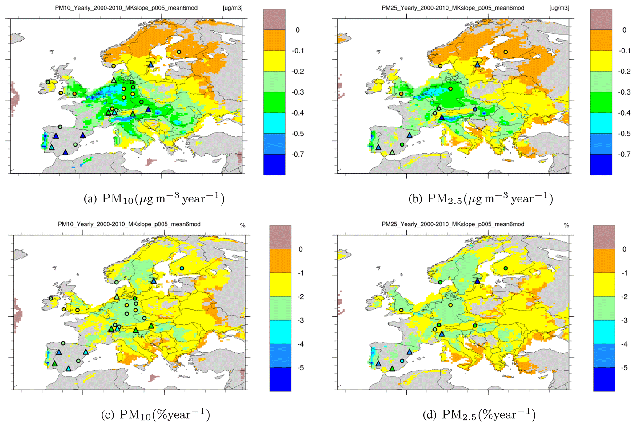
Figure 2Mean Sen slopes for PM10 and PM2.5 trends in 2000–2010: absolute (a, b) and relative (c, d) slopes calculated by the six-model ensemble (described in Colette et al., 2017a), Appendix A3. Modelled trends – coloured contour map (grey or white means non-significant trends); observed trends – coloured triangles (significant) and circles (non-significant).
The model results over the simulation domain and the observations at the trend sites show overall decreasing trends of PM10 and PM2.5 levels between 2000 and 2010. The modelled mean decreasing trends vary over the studied domain from below 0.1 µg m−3 yr−1 in northern Europe to 0.1–0.3 µg m−3 yr−1 in the eastern parts and to 0.3–0.5 µg m−3 yr−1 in central Europe and most of the UK, with PM2.5 downward trends being just slightly smaller than those for PM10. Starting from the concentration levels in 2000, the mean relative decreasing trends range mostly from 0.1 % yr−1 to 0.3 % yr−1 for PM10 and PM2.5. Compared to the distribution of absolute trends, steeper slopes of relative decreasing trends are also seen in the southern parts of Fennoscandia in addition to central Europe and the UK.
The six-model simulated mean trends are in general comparable to the observed ones, but some discrepancies are still seen in their geographical distribution. For instance, quite strong decreasing trends for PM10 and for PM2.5 are observed at three of the Spanish sites, while the model ensemble hardly indicates any significant trends over Spain. It should be noted that the models do calculate negative PM trends for the Spanish sites (as seen in Fig. A7), but due to considerable inter-annual variability, most of them are not identified as significant. Furthermore, the models calculated the strongest decreasing trends of 0.5–0.7 µg m−3 yr−1 for PM10 and PM2.5 in Portugal and Benelux, but no measurements were available to validate the modelled results. For Germany, the slopes of observed trends are similar to or somewhat lower than the modelled ones, but unlike the model results, none of the observed trends was identified as significant. In the next sections, the trends at the individual monitoring sites will be considered more closely.
Figure 3 illustrates the inter-model variability in PM trend slopes, showing the coefficient of variability (COV) of the trends simulated by the individual models relative to the ensemble mean (standard deviation – SD/ensemble mean) for PM10 and PM2.5. The COV is somewhat larger for the modelled PM10 trends compared to those for PM2.5. This reflects larger uncertainties in modelling the coarse fraction of PM, which is mostly due to natural origin, i.e. sea salt and windblown dust. As shown in Table A, the models used different parameterizations for the source functions of natural aerosols (also, some of them did not include online simulations of windblown dust but only mineral dust from boundary conditions).
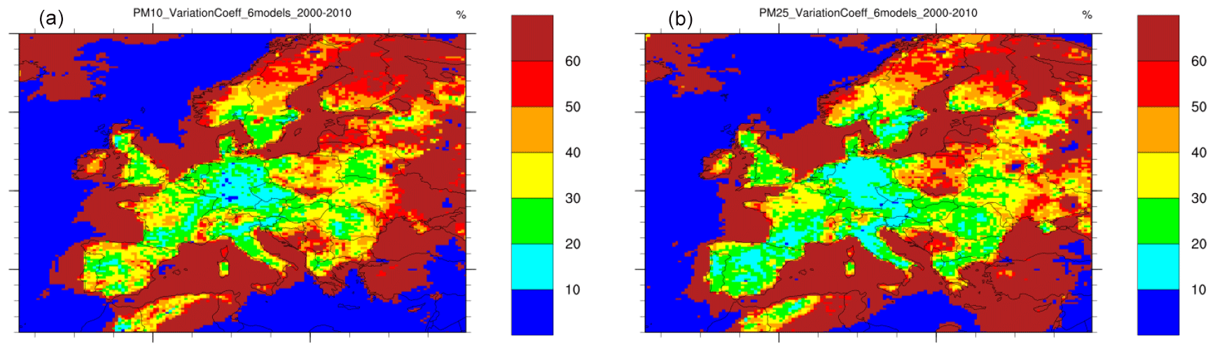
Figure 3The coefficient of variation of PM10 (a) and PM2.5 (b) trends simulated with the individual models relative to the six-model ensemble mean for the period 2000–2010.
The lowest spread in the modelled trends (below 20 %) appears in central Europe (Germany, Czech Republic) and also parts of Spain, northern regions of Italy and in the very south of Scandinavia for PM2.5. Those regions correspond to the strongest simulated PM trends. Otherwise, the COV is 20 %–40 % over most of Europe, increasing to 40 %–60 % in Poland, western and northern Fennoscandia, the Baltic countries and parts of Russia, where the modelled trends are relatively low or insignificant.
The maps with annual mean PM10 and PM2.5 trend slopes calculated by the individual models are provided in the Appendix. Figures A3 and A4 show the Sen slopes of PM10 and PM2.5 simulated by the six models and the observed trends for the period of 2000–2010. The significant modelled slopes are in general quite close to each other, indicating decreasing trends from 2000 to 2010. Also, the spatial variability of the Sen slopes in the individual models' results shows much similarity, with the strongest decreasing trends identified in central Europe (in particular in the Benelux countries and Germany). EMEP and LOTO calculated respectively the largest and weakest negative mean trend slopes as well as the largest and smallest fractions of the modelling domain with significant PM trends, namely 45 % and 57 % of grid cells according to EMEP and 17 % and 38 % according to LOTO for respectively PM10 and PM2.5, with the results from the other models lying between those values. As most of the input and set-up for the model runs was harmonized (Sect. 2.1), the differences we see here are due to differences in model configurations and process descriptions (see Table A), leading to different responses of the models to the changes in emissions and inter-annual meteorological variability. Differences in the formulations of secondary aerosol formations (inorganic and organic) can be pointed to as very important reasons for discrepancies in PM modelled trends. Differences in aerosol removal, in particular wet scavenging efficiency, also play a certain role (besides LOTO and MATCH being driven by different meteorology). Further note that the models have a different thickness of the lowest layer, which affects the concentrations, removal and transport distances of primary PM and its gaseous precursors.
Relative to the year 2000, all the models simulate stronger trends for PM2.5 compared to PM10, as seen in Figs. A5 and A6. This is to be expected as the natural contribution, which is strongly meteorology dependent, is greater in PM10. The distribution patterns of relative trends from the models are in general similar to those for the corresponding absolute trends. However, there is a difference between the models in the locations of their strongest simulated relative trends, namely in central Europe (e.g. EMEP, MINNI, POLR) or in northern Europe (e.g. CHIM, LOTO, MATCH). The fraction of the EDT domain with significant PM trends simulated with the individual models ranges from 17 (LOTO) to 45 (EMEP) % for PM10 and from 38 (LOTO and MINNI) to 57 (EMEP) % for PM2.5.
Figure 4 presents observed and modelled annual mean series of PM10 and PM2.5 at the trend sites for the period 2000–2010. Shown are the mean values from the six-model ensemble (dotted curves in Fig. 4a) and from the individual models' results (Fig. 4b and c). Note that the year of 2000 is a gap year at 7 out of 26 sites for PM10 and at 8 out of 13 sites for PM2.5, as described in Sect. 2.2. In particular, none of the Spanish sites is included for 2000, bringing some inconsistency in site-averaged PM10 and PM2.5 annual mean series.
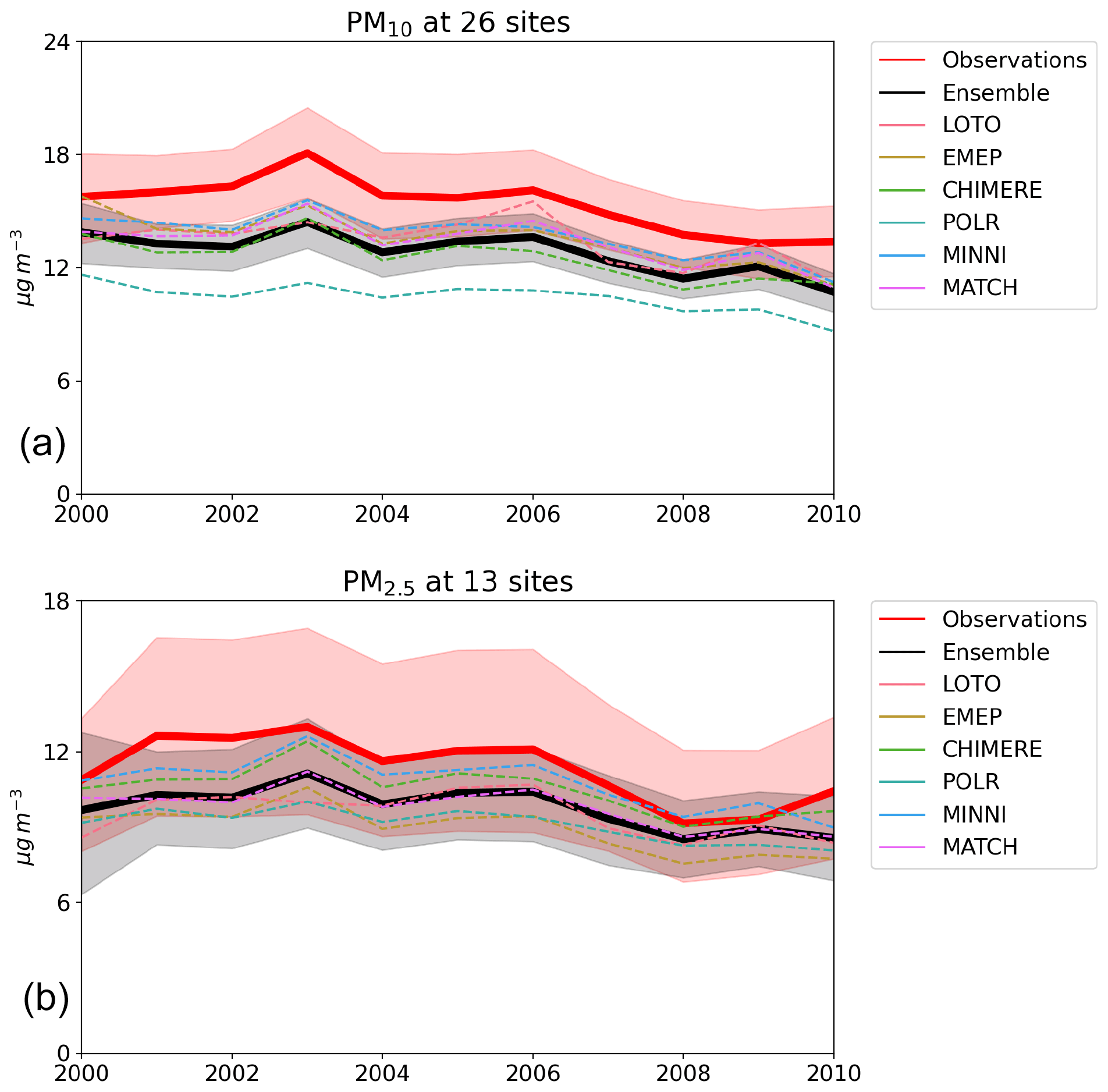
Figure 4Observed and simulated with the six-model ensemble and the individual models' annual mean concentrations of PM10 (a) and PM2.5 (b) for the period 2000–2010, averaged over the trend sites. The 95 % confidence intervals for observed and ensemble modelled PM concentrations are shown with shaded areas. The number of sites with available observations for the individual years can be found in Table 1. (Note: PM10 from POLR does not include coarse sea salt; see the text for explanations.)
Although they are underestimated with respect to the observations, the annual mean concentrations of PM10 and PM2.5 from the six-model ensemble follow the observed year-to-year PM variations well, with a peak in 2003 and a smaller one in 2006 (the years with heatwave occurrences, which facilitated enhanced photo-chemical formation of sulfate and secondary organic aerosols and inhibited aerosol wet removal). Furthermore, the observations show a trend stagnation for PM10 and an increase in PM2.5 towards the end of the period at the sites considered. This is not reproduced accurately by the models. A look at the individual sites reveals that the observed increase is the result of PM2.5 going up from 2008/09 to 2010 at 7 out of 13 sites. According to assessments of PM pollution in 2009 and 2010, presented in EMEP Status Reports 4/2011 and 4/2012 (https://www.emep.int/, last access: 1 November 2021), about half of the sites with PM measurements reported an increase in annual mean PM10 and PM2.5 with respect to the year before. As documented in those reports, a 3 %–4 % decrease per year in PM10 was registered between 2008 and 2010, whereas average PM2.5 levels were similar in 2008 and 2009 and increased by 4 % in 2010, averaged over all the sites with PM data. However, large variations between monitoring sites were observed. For instance, enhanced annual mean PM10 and particularly PM2.5 levels were reported for 2010 at Austrian, German, Swiss, and Finnish sites, which are among the trend sites included in the present trend analysis. The major reason for elevated annual PM levels is often the occurrence of winter pollution episodes (caused by stagnant conditions within a very low boundary layer and exacerbated by enhanced emissions from domestic heating), which are not always accurately modelled due to either an overestimation of mixing layer height by relatively coarse vertical resolution or/and underestimation in the emission input data.
In general, the EDT model ensemble reproduces the observed annual 2000–2010 series of PM at the trend sites quite well, showing a high correlation of 0.95 for both PM10 and PM2.5. Overall, the ensemble-simulated PM10 and PM2.5 concentrations are lower than observed values by 31 % and 19 % respectively (a greater bias for PM10 is partly caused by the POLR model – see below). A fairly good correspondence with respect to PM year-to-year changes is seen in Fig. 4b and c for the individual models compared to observations (with the exception of PM10 concentrations from POLR having a low bias because the contribution from coarse sea salt was not accounted for). Some deviations of LOTO's results for 2003 and 2006 are probably due to a different meteorological driver used in the model runs (see Sect. 2.1). The correlation between the modelled and measured series of annual mean PM10 and PM2.5 is high, with the following correlation coefficients: 0.96 and 0.93 for CHIM, 0.93 and 0.93 for EMEP, 0.77 and 0.85 for LOTO, 0.93 and 0.90 for MATCH, 0.93 and 0.88 for MINNI, and 0.70 and 0.87 for POLR for PM10 and PM2.5 respectively. These results give credibility to the results of the models and their ability to accurately simulate the changes in the PM levels due to emission changes and to represent the inter-annual variability due to meteorological conditions. These results also show that the model ensemble correlates better with the observations than the individual models when both PM10 and PM2.5 annual series are considered.
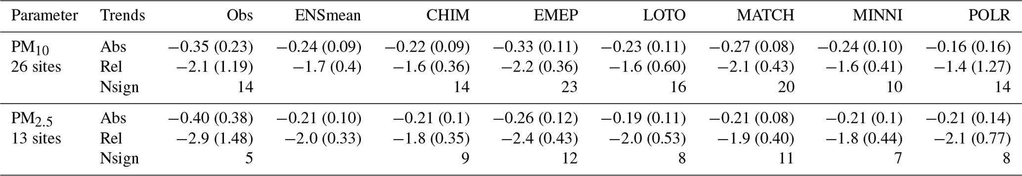
Averaged over all the sites (see Table 1), the mean ensemble-simulated trends (SDs are in parentheses) are −0.24 (SD = 0.09) µg m−3 yr−1 for PM10 and −0.21 (0.10) µg m−3 yr−1 for PM2.5. These are smaller compared to the observed −0.35 (SD = 0.35) and −0.40 (0.38) µg m−3 yr−1 respectively but can be anticipated given the models' underestimation of PM concentrations. The correspondence between model results and observations is better in terms of relative 2000–2010 trends (the SDs are in parentheses), which are −1.7 (0.40) % yr−1 and −2.0 (0.33) % yr−1 from the model ensemble and −2.1 (1.19) % yr−1 and −2.9 (1.48) % yr−1 from the observations for PM10 and PM2.5 respectively.
Table 1Observed and modelled (ensemble mean and individual models) PM10 and PM2.5 annual mean trends for the period 2000–2010, averaged over all trend sites. The standard deviation is included in parentheses. Units are µg m−3 yr−1 and % yr−1 for absolute (Abs) and relative (Rel) trends respectively. The number of sites with significant trends identified by observations and models (Nsign) is also provided.
5.2 PM trends at the individual sites
Figure 5 presents observed and simulated (by the six-model ensemble) PM10 and PM2.5 trend slopes for each site for the period 2000–2010. The sites at which significant trends were observed are marked with a star. The modelled significant and insignificant trends are represented respectively by dark and light blue bars.
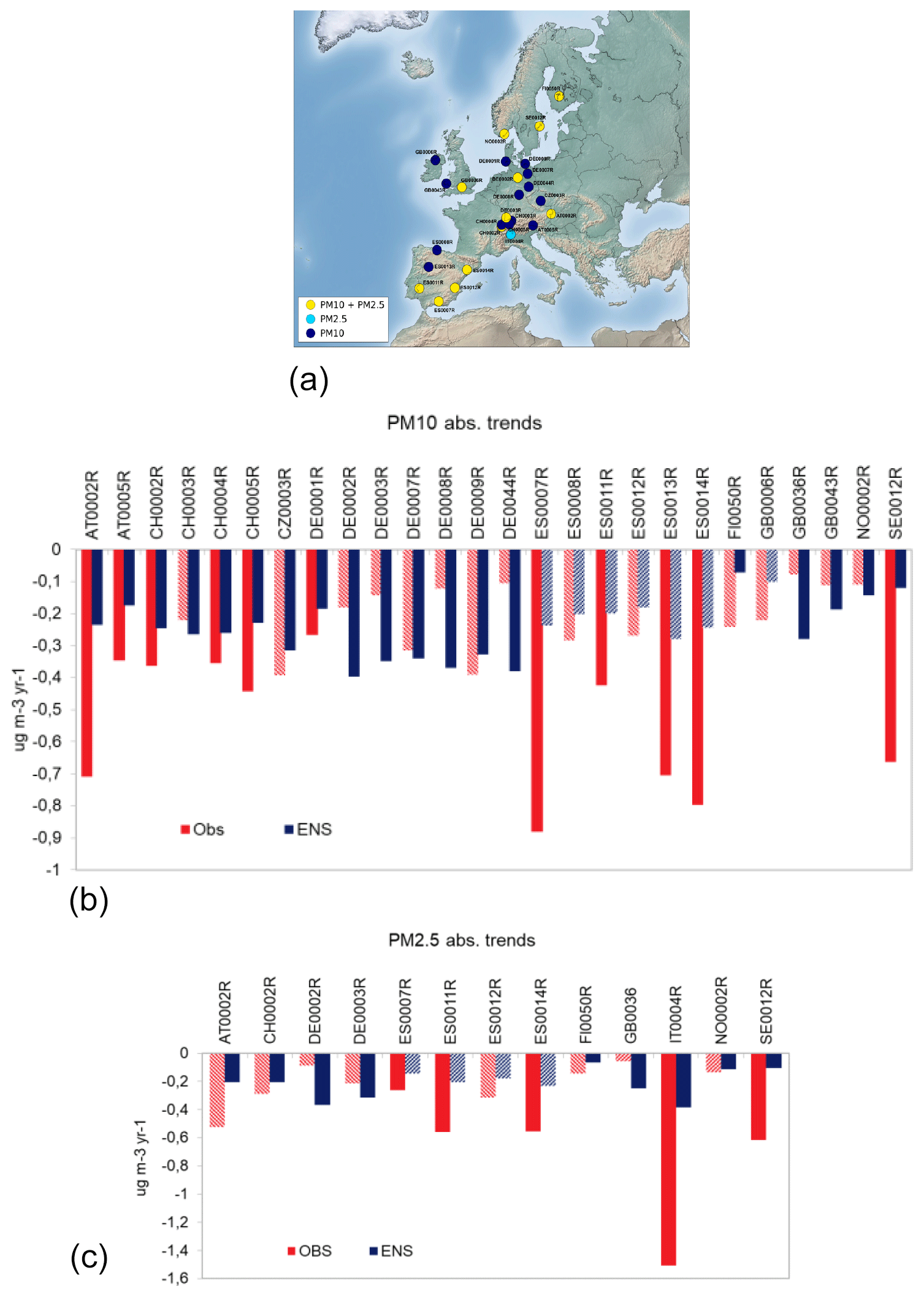
Figure 5Observed and modelled (six-model ensemble) trend slopes (µg m−3 yr−1) for the period 2000–2010 at the trend sites for PM10 (b) and PM2.5 (c). Significant modelled trends are shown in dark blue, non-significant ones in light blue. Sites with non-significant trends are represented by striped bars. The trend sites are shown on the map (a).
The observed and ensemble-modelled PM10 and PM2.5 trends at all the sites are decreasing. Figure 5 shows quite a large variability in the trends observed at different sites, ranging between −0.08 and −0.88 µg m−3 yr−1 for PM10 and between −0.05 and −1.5 µg m−3 yr−1 for PM2.5. Compared to the observations, ensemble-modelled trend slopes show less variability across the sites, with the standard deviations of 0.09 and 0.10 µg m−3 yr−1 versus 0.23 and 0.38 µg m−3 yr−1 in the observations for PM10 and PM2.5 respectively (Table 1). The modelled trends are mostly within −0.5 µg m−3 yr−1 and rather poorly correlated with the observations between the trend sites. The strongest negative PM10 trends were observed at three of the Spanish sites and one Austrian site (with decreases greater than 0.7 µg m−3 yr−1), while the weakest (and mostly non-significant) trends were registered at British, Norwegian and some German sites (below −0.15 µg m−3 yr−1). The strongest significant PM10 decreasing trend slopes were modelled for German and some other sites in central Europe. For most of the Spanish sites, the model-ensemble-simulated PM decreases by 0.2–0.3 µg m−3 yr−1, but the trends were classified as insignificant. In general, we see a similar pattern in the results for PM2.5, with the exception that the strongest trend was both observed (−1.5 µg m−3 yr−1) and modelled (−0.4 µg m−3 yr−1) for Ispra (IT0004) in the Po Valley. Uncertainties in the emission trends and spatial distribution could be one of the main reasons for the discrepancies between the model ensemble and observations (see Sect. 7 for more discussion).
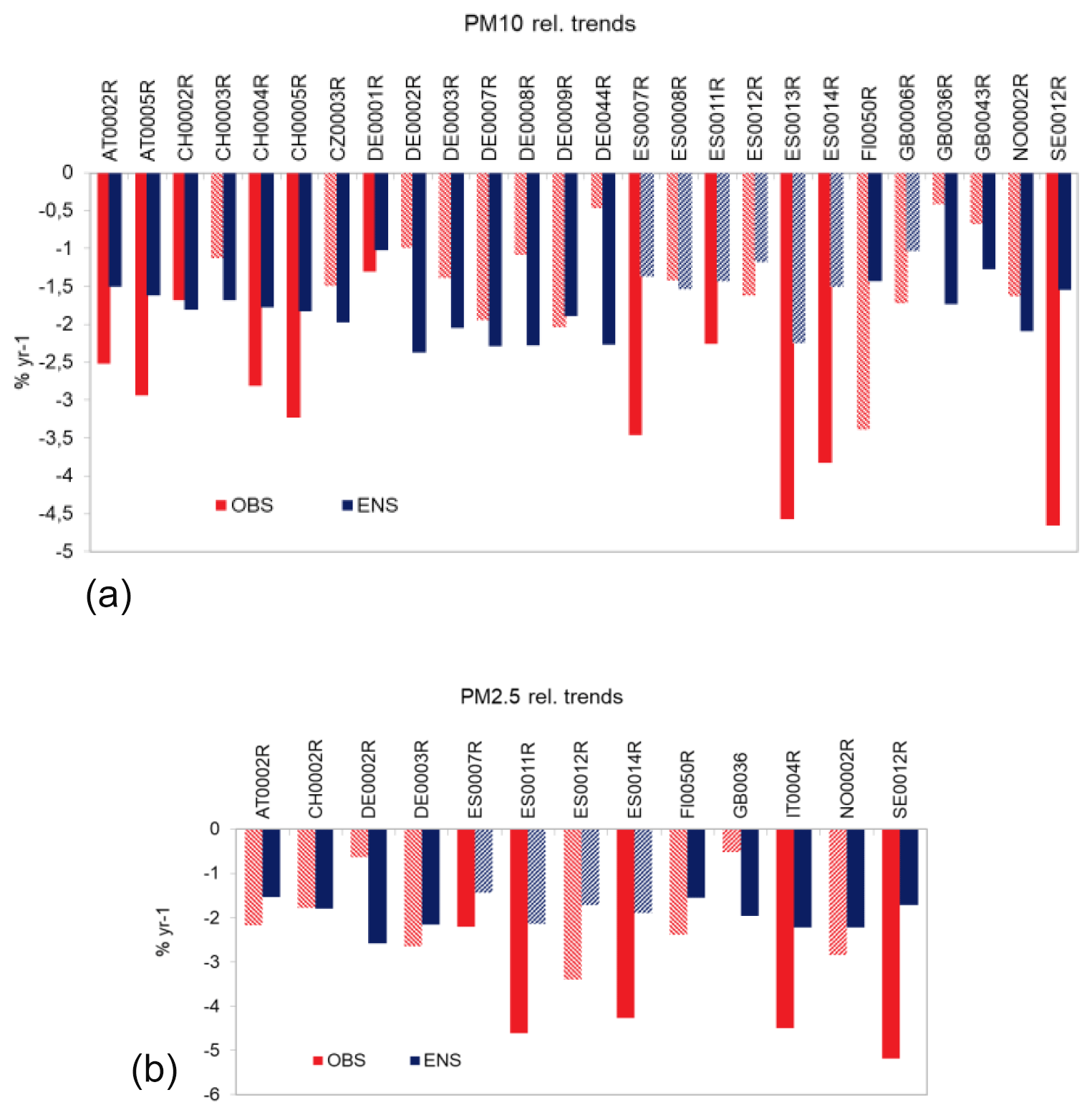
The observed relative trends range from −0.5 % yr−1 to −4.5 % yr−1 for PM10 and from −0.5 % yr−1 to −5.2 % yr−1 for PM2.5 (Fig. 6). Also in this case, ensemble-simulated relative trends show less variability, with values between −1.0 % yr−1 and −2.5 % yr−1. The strongest negative PM10 trends (with rates of decrease greater than −3.5 % yr−1) were observed at three of the Spanish sites and the Swedish one, whereas the weakest and mostly non-significant trends (under −1 % yr−1) were registered at the British and some German sites. The reason indicated in the previous paragraph for model–observation differences also applies for relative trends, but for the latter the estimated PM at the start of the period (see Sect. 2.3) affects the results as well.
All in all, the observations show significant PM10 trends at 11 out of 26 sites and significant PM2.5 trends at only 5 out of 13 sites. A closer look at PM10 and PM2.5 annual series at the individual sites (not shown) reveals that the sites where no significant trend was identified in the observations have a particularly large inter-annual variability of PM concentrations. Model ensemble results identify significant trends at more sites compared to the observations, namely at 18 sites for PM10 and at 8 sites for PM2.5. As can also be seen on the trend maps (Fig. 2), the model ensemble and the observations do not always agree regarding the significance of trends at specific locations, even within the same country. For example, in Spain, strong decreasing significant trends were observed at four out of six sites for PM10 and at three out of four sites for PM2.5, whereas the model ensemble mostly estimates non-significant trends. This is in contrast to the German sites, for which the models simulate significant and quite appreciable PM10 and PM2.5 trends for all the sites (as a result of emission reductions in the whole country), but significant observed trends are found for only one out of seven sites for PM10 and for neither of two sites for PM2.5. The reason for this seems to be that the trends were distorted by particularly high annual mean PM concentrations in 2003, 2006 and 2010 at most of the German sites (not shown here).
Similarly to Fig. 5 for the model ensemble, Fig. A7 presents PM10 and PM2.5 mean trends calculated by the individual models, with only significant modelled trends shown. For any specific site, the trend slope values from the models are in general agreement (Fig. A7), while there are discrepancies between the models with regards to the significance levels of simulated trends. The largest number of significant PM10 and PM2.5 trends were simulated by EMEP (23 and 14 respectively) and the smallest number by MINNI (10 and 7) (see also Table 1).
The relative trends from the individual models are compared to each other and to observed relative trends in Fig. A8 for the set of trend sites.
Averaged over all the sites (see Table 1), the trends simulated with the individual models range from −0.16 to −0.33 µg m−3 yr−1 for PM10 and from −0.19 to −0.26 µg m−3 yr−1 for PM2.5 and are weaker than observed trends (−0.35 and −0.40 µg m−3 yr−1 respectively). The agreement among the models appears to be better in terms of relative trends that range from −1.4 % yr−1 to −2.2 % yr−1 for PM10 and from −1.8 % yr−1 to −2.4 % yr−1 for PM2.5 (site averages). Compared to absolute trends, those correspond better to observed trends (−2.1 % yr−1 and 2.9 % yr−1 respectively).
5.3 PM seasonal trends
Figure 7 presents the maps of 2000–2010 seasonal mean trends of PM10 and PM2.5 from the six-model ensemble and the observations. For the winter season, the model ensemble estimates significant PM10 and PM2.5 trends only in small areas, mostly in southern parts of Europe. The observational data do not show any significant trends for PM10. For PM2.5, the observations indicate quite strong significant trends at only three sites, i.e. in the north-east of Spain (also identified by the model ensemble), north of Italy and south of Sweden. Probable reasons for the limited number of sites with significant observed trends are negligible reductions and even increases in the emissions of primary PM from residential heating, most important in the winter period, which were not efficiently regulated.

Figure 7Mean Sen slopes for PM10 and PM2.5 seasonal trends for 2000–2010, calculated by the six-model ensemble (see Fig. 2 for explanation).
For the summer period, both the model ensemble and observations estimate the strongest negative trends out of all the seasons. Significant trends are simulated for most of the domain (except northern Europe, the south of Spain and most eastern parts of the domain). The number of sites with observed significant trends is also strongest for summer, namely 12 out of 26 for PM10 and 10 out of 13 for PM2.5. In the spring and autumn periods, both modelled and observed trend slope values and the fraction of sites with significant trends are between those of winter and summer.
It can be noted that Ispra in northern Italy (IT0004) is the only site where significant PM2.5 trends were observed and modelled for all seasons, with the exception of the modelled winter trend. For PM10, the quite strong significant mean trends at four Spanish sites (ES0007, ES0008, ES0013 and ES0014) appear to be due to strong summer trends, whereas the trends are insignificant in the other seasons. Among the German sites, significant observed PM10 trends are only identified at DE0001 and DE0007, and only for the spring period. The models agree with that but also calculate significant trends for summer and autumn.
Figure 8a and b present the annual series of the six-model ensemble and observed seasonal mean trends of PM10 and PM2.5 for the period 2000–2010, averaged over all the trend sites. The values of absolute and relative trend slopes are summarized in Table 2.
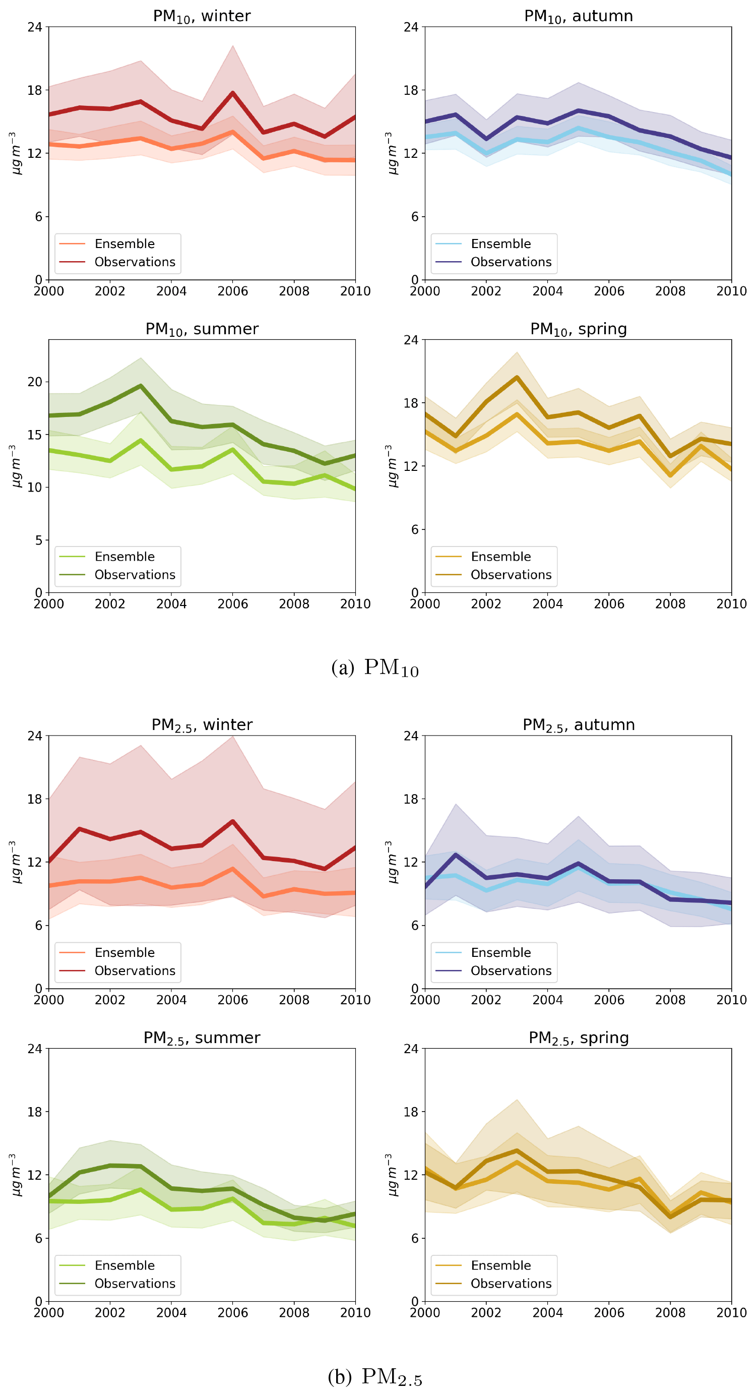
Figure 8Changes in seasonal mean PM10 and PM2.5 concentrations in the period 2000–2010, averaged over the trend sites, observed and simulated with six-model ensemble. The 95 % confidence intervals are shown with shaded areas. The number of sites with available observations for the individual years can be found in Table 2.
Table 2Observed (Obs) and modelled (six-model ensemble; ENS) mean seasonal trends and standard deviations (in parentheses) for 2000–2010 at all the trend sites. Units are µg m−3 yr−1 and % yr−1 for absolute (Abs) and relative (Rel) trends respectively. The numbers of sites with significant trends are given in square brackets.
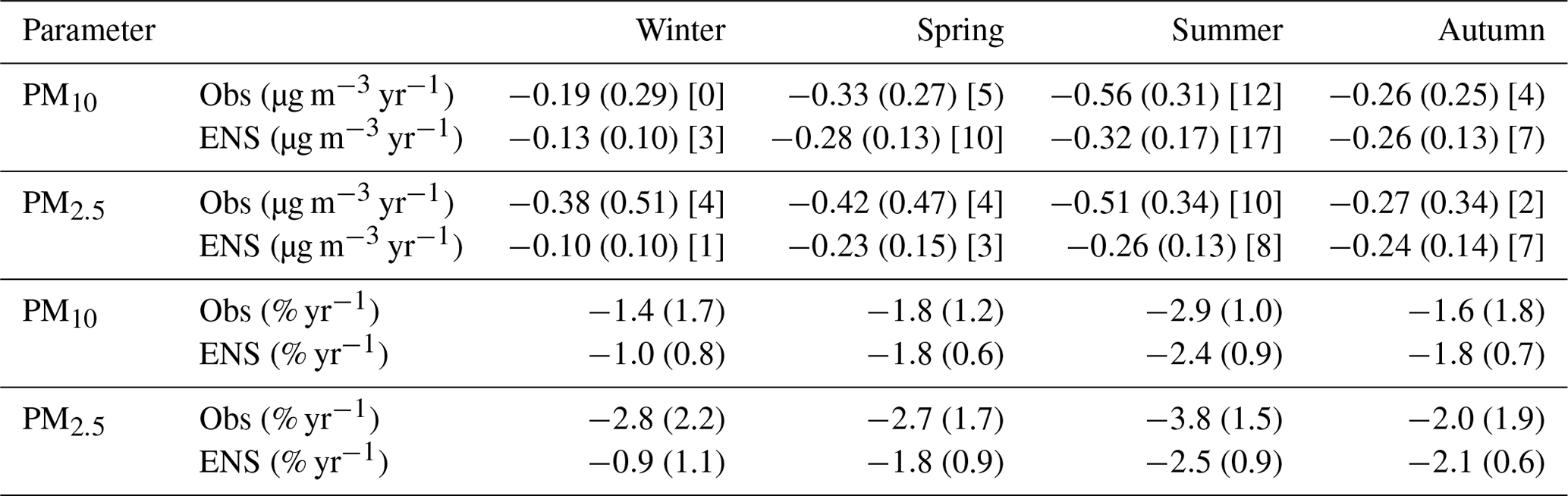
Averaged over the trend sites, the largest decrease in PM during the 2000–2010 period took place in the summer months for both PM10, with the mean seasonal trend of −0.32 µg m−3 yr−1 from the model ensemble and −0.56 µg m−3 yr−1 from the observations, and PM2.5 (−0.26 and -0.51 µg m−3 yr−1 respectively). The weakest trends were found for the winter season from the models and observations for PM10 (−0.13 and −0.19 µg m−3 yr−1 respectively) and also for modelled PM2.5 (−0.10 µg m−3 yr−1), whereas the observed PM2.5 trend has a minimum of −0.27 µg m−3 yr−1 in the autumn season. The weakest winter trends are partly due to the larger amplitudes of the inter-annual changes in mean PM levels. In particular, the elevated winter levels of PM10 and PM2.5 in 2006, and especially in 2010, contribute to reducing the mean seasonal trend.
Figure 9 presents the seasonal mean trends simulated by the individual models and the model ensemble, along with the observed trends. The graphs nicely visualize the seasonal variations of PM trend slopes discussed above. They also show quite a good correspondence between the trend seasonality from the individual models. Relative trends of PM show quite similar seasonal patterns, with the strongest trends in the summer and weaker ones in the cold seasons of 2000–2010 (Fig. 9). For PM10, observed relative trends are −2.9 % yr−1 in the winter period and −3.7 % yr−1 in the summer period; the respective numbers from the model ensemble are −2.3 % yr−1 and −2.5 % yr−1. For PM2.5, the observed and modelled summer trends are −3.7 % yr−1 and −2.9 % yr−1, whereas the weakest observed mean trend of −2.0 % yr−1 was in the autumn and the weakest modelled trend of −1.4 % yr−1 was estimated for the winter period. The individual models largely agree on the seasonal profiles of the relative trends, although some variability exists between the simulated trend slopes (similar to those for seasonal absolute trends).
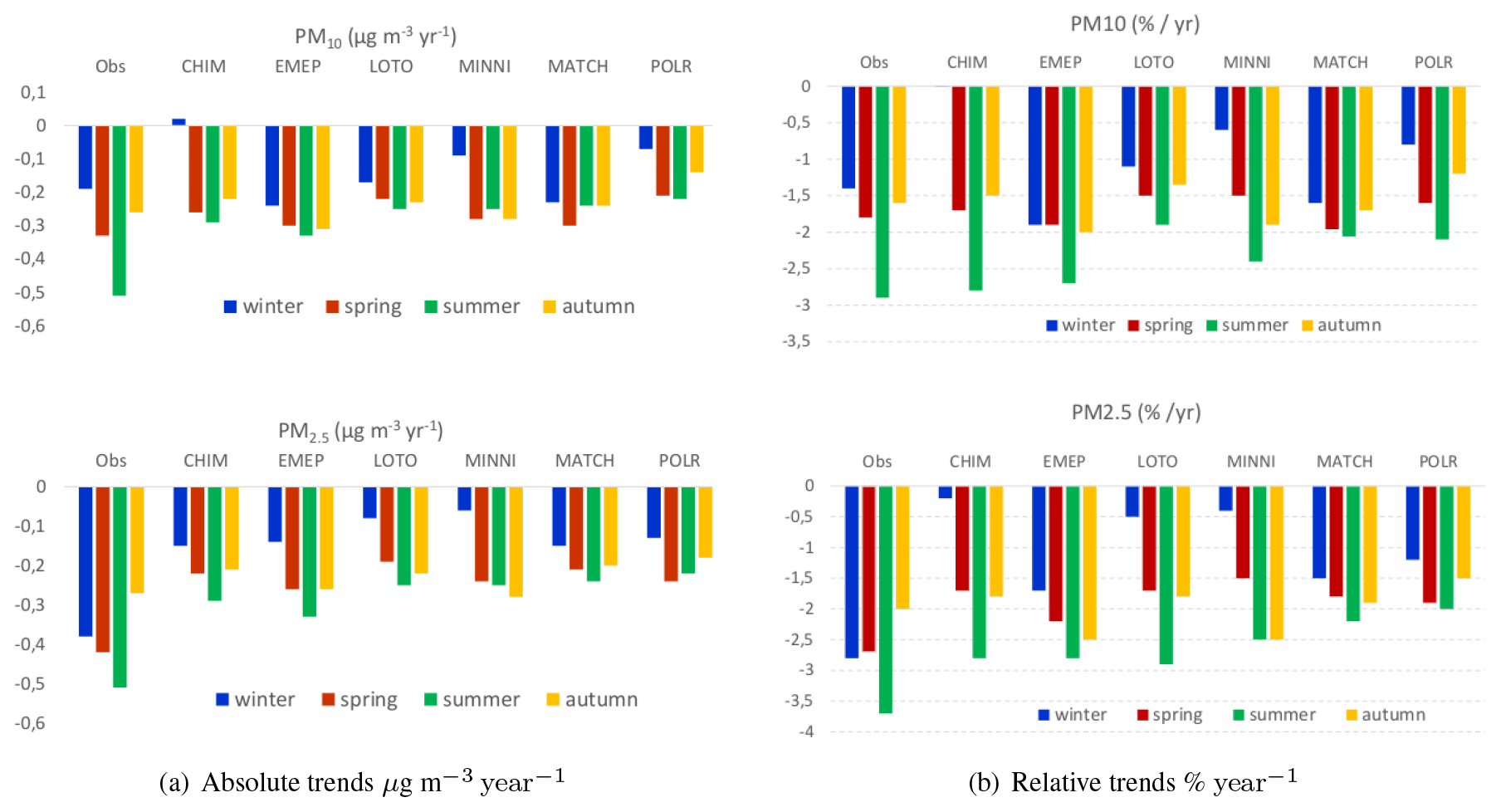
Figure 9Mean relative seasonal trends in the period 2000–2010 at the trend sites for PM10 and PM2.5: the trends from the observations, the individual models and the six-model ensemble are shown.
5.4 Contribution of individual components to PM trends
PM10 and PM2.5 are a complex mixture of different aerosol components originating from a variety of anthropogenic and natural emission sources, and so PM trends are basically the sum of individual trends of its constituents. Thus, for a better understanding of the effects of emission reductions of different pollutants, it is imperative to look at the role of the individual aerosol components in the changes in PM concentrations.
A comprehensive study of the trends for individual aerosols is beyond the scope of this paper. Besides, there are practically no available observational data for individual PM components collocated with PM measurements during the period 2000–2010. In fact, Birkenes in the south of Norway is the only site for which observational data for both PM10 and PM2.5 and for secondary inorganic aerosol (SIA) meet the required criteria for the trend study. Still, we think that, for a better interpretation of PM trends discussed in this paper, it is relevant to have a brief insight into the trends of PM components. Here, we summarize the main results of modelled and observed trends of some PM components for 2000–2010. For a more detailed analysis of inorganic gases and aerosols, the reader is referred to Ciarelli et al. (2019).
Figure A9 shows the maps of model-ensemble-simulated and observed annual mean 2000–2010 trends for , and aerosols. Note that, due to the lack of consistent observational datasets (as pointed out above), the set of sites for SIA is not the same between the species and is also different from those used in PM trend analysis. The number of sites used here is 39, 14 and 13 for , and .
The absolute trends are all decreasing, though the rates are not directly comparable (since they are expressed as µg m−3 (S) yr−1 and µg m−3 (N) yr−1). The maps of relative trend slopes show the strongest trends all over Europe for (between −2 % yr−1 and −4 % yr−1 over most of the domain, exceeding −5 % yr−1 in Spain), closely followed by . For , the models only estimated significant downward trends in central European countries and Italy. The modelled trends for SIA are decreasing over the entire domain, whereas the observations indicate significant increasing trends of and at the Polish site Sniezka (close to the Czech border). In addition, rather strong, though non-significant, positive trends of and were observed at two Dutch sites and somewhat weaker positive trends at a few other sites. No observational datasets long enough (or obtained with consistent analytical methods) for trend studies of carbonaceous aerosols were available at EMEP sites. Shorter series for total carbon, available for three to four sites, show a 4 %–5 % decreasing trend between 2003/04 and 2010.
In summary, the results presented here and the analysis by Ciarelli et al. (2019) indicate that the models estimate a somewhat larger than observed decrease in in central (also missing some positive trends) and northern Europe and a smaller decrease in Spain. The models appear to overestimate the observed negative trends for and also for , though to a smaller degree (one should keep in mind that for and there is a limited number of measurement sites covering a limited geographic area). It should be noted that none of the models accounts for base cations (i.e. Na+, K+, Ca2+ and Mg2+) in gas–aerosol partitioning of HNO3 (see Table A). Those base cations are significant components of sea salt and mineral dust. They participate in aerosol chemistry and facilitate the formation of coarse , consuming HNO3 and thus making less of it available for NH4NO3 formation. As the emissions of sea salt and mineral dust strongly depend on meteorology (especially on surface wind speed), formed on the base cations (and consequently total ) is subject to inter-annual variability, which could weaken trends and lead to a larger fraction of insignificant trends. Thus, not including base cations in aerosol chemistry could be one reason for model overestimation of the observed trends (see also the discussion in Sect. 7. Among the EDT models, MINNI and POLR did not include coarse , CHIM and LOTO included formation on sea salt Na+, while EMEP and MATCH used constant reaction rates for coarse formation from HNO3, irrespective of base cation availability (Table A). However, we could not see any consistent differences in the relative trends of and between the models with and without coarse (not shown here): the comparison of trends from the individual models to observations at the rather limited number of sites did not give conclusive results.
The relative contributions of , , , total primary particulate matter (TPPM10) and anthropogenic SOA (ASOA) to PM10 trends in the period 2000–2010 estimated by the model ensemble are presented in Fig. 10. The maps reveal considerable variability in the role of the individual aerosol species PM10 trends across European countries. The decrease in concentrations (Fig. 10a) played the dominating role over most of the EDT domain, except from parts of central Europe and northern Italy. That is, relatively large contributions of to PM10 trends are seen in Germany (and neighbouring parts of France, the Czech Republic and Poland), Denmark, the Netherlands, and the Po Valley (Fig. 10c). The reduction of levels, which includes both ammonium sulfate and ammonium nitrate, appears to be quite an important contributor to the PM10 decreasing trends, with the largest effects estimated for Poland, Denmark, and the Po Valley (Fig. 10b). The reduction of primary PM emissions was, according to the model ensemble simulations, the dominating factor for PM10 trends in Portugal and the southern parts of the Balkans as well as in many European cities (due to emission reductions from traffic and residential heating) (Fig. 10d). Finally, ASOA is also estimated to have quite a notable contribution of 3 %–7 % to PM10 downward trends (though ASOA modelling is still associated with rather large uncertainties). The model results imply that the chemical composition of European PM10 has changed somewhat during the 2000–2010 period, with (and probably ASOA) becoming an increasingly important constituent compared to the other anthropogenic aerosols, i.e. , and primary emitted PM (elemental and primary organic carbon, dust and metals).

Figure 10Model-ensemble-simulated relative contribution to PM10 2000–2010 trends from anthropogenic aerosols, , , , total primary TPPM10 (except POLR) and anthropogenic SOA (except LOTO), and from natural aerosols, biogenic SOA (except LOTO), sea salt (except POLR) and mineral dust particles (except MATCH). Note that a different colour scale is used for the natural aerosols.
The relative contributions of , , and ASOA to PM10 trends in the period 2000–2010, as calculated by the individual models, can be found in the Appendix (Fig. A11). Most of the models (except for POLR) agree that, over most of the EDT domain, except from some central European countries, decreases in concentrations were the main cause of PM10 downward trends, with somewhat smaller contributions from decreasing levels. This is consistent with the emission trends shown in Fig. A1. The largest emission reductions were achieved for SOx, which explains the relatively strong trends in (and also appreciable trends in in the form of ammonium sulfate) concentrations. The reductions of NOx and NH3 emissions from 2000 to 2010 were smaller compared to . Thus, as the formation of ammonium sulfate was decreasing in the 2000s, more and more NH3 was becoming available for the formation of ammonium nitrate NH4NO3. Notably, in Germany as well as in the Benelux countries and the Po Valley, is estimated by the models to have the largest contribution to the PM10 trends. However, it should be kept in mind that in the regions influenced by mineral dust and/or sea salt, some nitric acid would be consumed in the formation of associated with base cations (as discussed above, this is not fully accounted for in the EDT models), so that less NH4NO3 would be formed compared to what the EDT models simulate.
Furthermore, the estimates by LOTO point to primary anthropogenic PM10 as the main component driving PM10 levels down in a large part of the simulation domain. CHIM, MINNI and to some extent EMEP agree with the LOTO estimates for northern Europe and the area covering Benelux, the northern parts of Germany and France, and the south of the UK. In contrast to the other models, POLR estimated that contributed the most to the PM10 trends, whereas the contributions of and were rather moderate in central Europe, the UK, and the Baltic countries. The modelled contributions of ASOA to PM10 trends is below 5 % according to CHIM, MATCH and MINNI, whereas EMEP simulates contributions of 5 %–10 % and POLR 5 %–30 %. This variability can be explained by the different ways of handling SOA chemistry in the models. Furthermore, somewhat weaker PM trends from LOTO could probably be explained by not including SOA chemistry in these simulations. Similar results are seen with respect to the relative contributions of the individual aerosols to modelled PM2.5 trends between 2000 and 2010 (Fig. A12).
As far as natural aerosols are concerned, emissions are largely driven by meteorological conditions (e.g. by the surface wind in the case of sea salt and windblown dust, while the air temperature controls emissions of biogenic VOCs – precursors of biogenic secondary organic aerosol, BSOA). In addition, the generation of mineral dust is dependent on the availability of erodible (snow- and vegetation-free) soil and its moisture (which in turn depends on precipitation frequency and amount), whereas the temperature and salinity of seawater affect sea spray formation, though those conditions are less variable. Of course, similarly to anthropogenic aerosol, the transport and removal of the natural particles are determined by atmospheric dynamics and precipitation. In short, year-to-year changes in the concentrations of natural aerosols are driven primarily by inter-annual meteorological variability. Among natural aerosols, only formation of BSOA has some dependency on anthropogenic emissions, as BSOA can be formed from biogenic VOCs condensing on primary organic aerosols from anthropogenic sources. Thus, BSOA production is somewhat affected by the trend in PM emissions. In addition, as discussed above, the changes in formed from anthropogenic NOx emissions are in fact dependent on the variability of natural aerosols of sea salt and mineral dust.
Not all natural particles were calculated in a consistent way by all of the models. The missing components are BVOC from LOTO and MATCH, sea salt from POLR and only EMEP- and LOTO-simulated trends of windblown dust in the modelling domain, whereas the other models only included mineral dust from boundary conditions. Figure 10f–h present the computed contributions of natural aerosols estimated by the models, i.e. biogenic SOA, sea salt and mineral dust, to PM10 trends, where the negative contributions (blue colours) mean increasing trends in the natural aerosols.
The model ensemble simulated decreasing BSOA trends that contribute 1 %–3 % of PM10 decreasing trends over almost all the land area (Fig. 10f), with the largest contribution (5–10%) in Fennoscandia and north-western Russia. The contribution of sea salt trends (derived as 3.26 × sea salt Na, assuming 30.7 % sodium content in sea salt aerosols, the same as in seawater) to PM10 trends is, on average, 2 %–5 % over land and exceeds 10 % in areas influenced more by the sea and less polluted regions (Fig. 10g). Comparison of the modelled sea salt trend with rather sparse observations can be found in Fig. A10a.
Furthermore, from the EMEP and LOTO results, we see contributions of 1 %–3 % from mineral dust to decreasing PM10 trends over most of Europe (in excess of 10 % in Spain and Italy) but also some negative contributions due to increasing dust trends in Greece, Portugal and south-eastern Europe and Russia (Fig. 10h). All in all, the inter-annual variability and increasing modelled trends for natural aerosols for some regions do not appear to have reversed the decreasing PM10 trends in the 2000–2010 period (with some exceptions for windblown dust).
Model analysis of the seasonal trend of the individual PM10 and PM2.5 components shows the strongest trends of SIA (, and ) in summer and also in spring for , while the weakest trends of all SIA are calculated for winter. In contrast, the strongest trends for primary PM are simulated for winter and the weakest ones for summer.
As no regular measurements of PM were conducted prior to 2000, this paper mainly focuses on the period 2000–2010. As far as the years prior to 2000 are concerned, we have to rely solely on model simulations to assess the effect of emission reductions on European levels of particulate pollution in the 1990s. Given that, any deep analysis of that decade is beyond the scope of the paper, but still we think it is relevant to present a multi-model assessment of PM trends during the whole 1990–2010 period studied within the EDT framework. It should be kept in mind while looking at those results that the emission data, in particular for PM, are much less reliable before 2000.
Figure A13 shows annual mean trends for the period 1990–2010 for PM10 and PM2.5, absolute and relative to 1990, produced by the ensemble of five models (all the above except POLR). Over the whole European domain, the models simulate significant decreasing PM trends. The strongest trends (0.75–1.0 µg m−3 yr−1 or 2.5 % yr−1–3 % yr−1) were simulated for central Europe (extending eastward over Ukraine and European Russia for PM2.5). The weakest trends of less than 0.3 µg m−3 yr−1 (1.5 % yr−1–2 % yr−1) are seen in northern Europe and Russia and in southern Europe. The rest of the domain experienced intermediate trends of 0.3–0.75 µg m−3 yr−1 (1.5 % yr−1–2.5 % yr−1 relative to the year 1990). Notably, the weakest decreasing trends (below 1.5 % yr−1) are modelled for PM10 in the southernmost parts of Mediterranean countries, which are heavily influenced by Saharan dust and thus PM trends due to the reductions of anthropogenic emissions being distorted. The mean annual trends during the period of 1990–2010 are stronger compared to those for the 2000–2010 period (Fig. 2). This is a consequence of larger emission reductions in the 1990s compared to the 2000s. Thus, the EDT model ensemble simulated that annual mean PM10 and PM2.5 concentrations decreased by between 5 and 15 µg m−3 across most of Europe (by 2–5 µg m−3 in northern Europe) from 1990 to 2010.
6.1 PM trends in European countries in the 1990–2000–2010 periods
The graphs in Fig. A14 provide more details regarding PM10 trends in individual European countries and compare the trends in the 1990s and 2000s.
Figure A14a shows the trends of PM10 between 1990 and 2010 simulated by the five models for the individual countries and sea areas. The strongest annual mean trends, with decreases greater than −0.6 µg m−3 yr−1 (leftmost countries in the graph), were simulated for central European (Germany, Hungary, Czech Republic) and the Benelux countries, which were the regions with some of the highest PM levels. The weakest downward trends are modelled for relatively cleaner northern European (Iceland, Norway, Finland, Sweden) and Baltic countries but also in Mediterranean countries influenced by shipping emissions and African dust intrusions (rightmost countries in the graph). The models are in general agreement regarding the ranking of PM10 national trends, and the spread between PM national trends calculated with the individual models is rather moderate (the mean SD between the models is 0.054 µg m−3 yr−1, varying between 0.005 and 0.104 µg m−3 yr−1 for different countries). The variation of PM2.5 trends across Europe is quite similar (and therefore not shown here), with the only difference that the trends in the Benelux countries were strongest.
Figure A14b shows, for the individual countries and regions, the PM10 annual trends calculated by the model ensemble for the 1900–2000 and 2000–2010 periods separately. For most of the countries, the largest reductions of PM10 levels took place in the 1990s compared to the 2000s, which is consistent with considerably larger emission reductions of PM emissions and their gaseous precursors (except from ammonia) during the first of those decades. This is especially pronounced in central Europe, where the 1990–2000 trends were around 1 µg m−3 yr−1 compared to around 0.3 µg m−3 yr−1 in the 2000–2010 period. The exceptions are northern European countries and also relatively small emitters of pollution, such as Malta, Liechtenstein and Cyprus, where PM10 trends were similar during both decades.
The PM10 relative trends (i.e. with respect to the starting years of 1990 and 2000) in the 1990–2000 period are also considerably stronger than those in the 2000–2010 period (not shown, or in the Supplement). The model results indicate a large variability in 1990–2000 trends between the countries (from −1.1 % yr−1 in central Europe to −0.0–0.2 % yr−1 in northern Europe, Cyprus and Malta), whereas the 2000–2010 trends are more homogeneous across the countries, ranging between 0 % yr−1 and −3 % yr−1.
7.1 Discussion of the main results
The ensemble of six EDT models simulated that, from 2000 to 2010, the annual mean PM10 and PM2.5 concentrations decreased by between 10 % and 20 % over most of Europe and respectively by up to 25 % and 30 % in Germany, the Netherlands, Belgium, parts of the UK, Portugal, the north/centre of Italy and large parts of Scandinavia. Notably, despite lower PM2.5 concentrations, the PM2.5 absolute downward trends appear only slightly smaller than those for PM10, indicating a trend-masking role of coarse PM of natural origin. On average, we found a fair agreement between modelled and observed concentration reductions at 26 (for PM10) and 13 (for PM2.5) measurement sites. In the course of those 11 years, PM10 and PM2.5 concentrations at the studied sites decreased respectively by 17 % and 20 % according to the model ensemble and by 21 % and 29 % as derived from observational data. Moreover, we found a larger spatial variability of PM trends registered by observations compared to those estimated by the model, with observed decreasing trends ranging between approximately 5 % (at British site GB0036) and 50 % (at Swedish site SE0012). We also see some discrepancies in the geography of trends from the observations and EDT model, with the largest observed decreases (above 30 %) at the sites in Sweden, Finland and Spain (also the Po Valley for PM2.5), whereas the models simulate the strongest trends for German sites (mostly above 20 %) and do not identify significant trends for Spanish sites (though 10 %–20 % decreases in PM10 and PM2.5 are simulated).
Modelled PM concentrations are to a large degree determined by the emission data used, and modelled PM trends reflect the trends in national emissions. For instance, relatively strong simulated PM trends in Germany, Benelux, the UK and Portugal are due to considerable reductions of all gaseous precursors and primary PM in those countries (Fig. A2). Poland is among the countries with the greatest reduction of SOx and considerable reductions in NOx emissions from 2000 to 2010, but the increase in NH3 emissions contributed to additional SIA formation during those years. In addition, the emissions of primary PM2.5 in Poland increased during the same period. Thus, the resulting modelled downward trends are relatively weaker (and insignificant in parts of the country). In northern Europe, the appreciable decrease in PM concentrations is not only due to reductions in NOx and primary PM2.5 emissions in those countries, but is also due to decreased long-range transport from central Europe and the UK (somewhat lessened by the increased NOx emissions from international shipping in the North and Baltic seas). For Spain, the model ensemble simulated a substantial decrease in PM concentrations (though the PM trends were characterized as insignificant), mostly resulting from emission reductions of gaseous precursors, while the reductions in emissions of primary PM (especially coarse PM) were relatively smaller. Only the EMEP model (and MATCH for PM2.5) simulated significant PM trends for most of Spain, whereas PM trends from the other models were found to be insignificant due to smaller PM decreases from 2000 to 2010 or/and larger inter-annual variability (as in the results from LOTO and MATCH using a different meteorology).
Furthermore, the analysis showed considerable variability in the observed trends within the same country, which the models could not fully reproduce. This can be due to local emissions unaccounted for or misrepresented spatially and temporally in the model input. In some countries, the differences in trends could also be related to a complex topography leading to localized pollution transport dynamics (e.g. Switzerland and Austria), unresolved by meteorological drivers.
As PM is a complex pollutant, consisting of different aerosol species, the concentrations and trends of PM are the result of an intricate interplay of the effects of their direct emissions and gaseous precursors from a variety of anthropogenic and natural sources. As discussed in Sect. 5.4, the emissions of SOx went down by 37 % from 2000 to 2010, resulting in the decrease in ammonium sulfate concentrations and thus more ammonia available for reactions with nitric acid. The reduction of NOx emissions in the same period (17 %) was smaller than that of SO2. Given rather moderate reductions of NH3 emissions (only 6 % on average), the concentrations of ammonium nitrate decreased less compared to ammonium sulfate. The model ensemble calculated the decrease for to be in the range of 25 %–45 % (45 %–55 % in Spain and Portugal) and for in the range of 15 %–40 % over Europe from 2000 to 2010 (Fig. A9a–f). The modelled decrease in concentrations is mostly under 30 % and the trends are insignificant in most countries. For more detailed discussion on SIA trends, we refer the reader to the analysis published in Ciarelli et al. (2019). In that publication, relatively moderate trends in compared to the emission reductions of SO2 were explained by an increase in the availability of oxidant species and more efficient pH-dependent cloud chemistry resulting from those emission reductions. Ciarelli et al. (2019) also discuss a shift in the thermodynamic equilibrium between HNO3 + NH3 versus NH4NO3, favouring aerosol formation. Furthermore, the reduction of anthropogenic VOC emissions, including aromatic hydrocarbons – precursors of SOA – by 33 %, on average, led to a decrease in ASOA concentrations by 15 %–30 % from 2000 to 2010 (Fig. A9g and h). Finally, the emissions of both PM2.5 and coarse PM were reduced, on average, over the modelled domain by 10 %, thus making primary PM an important driver of PM10 and PM2.5 decreases in some European regions (not shown here).
Due to the lack of long-term observational data of PM10 and PM2.5 supplemented with chemical analyses, the model results regarding the role of the individual components in PM10 and PM2.5 trends during 2000–2010 cannot be thoroughly validated. We can only make a crude estimate, using observations of SIA and OC, which are not necessarily collocated, available at a limited number of sites. The observed average trends were strongest for organic aerosols (−3.8 % yr−1 at 4 sites), followed by (−2.9 % yr−1 at 13 sites) and (−2.6 % yr−1 at 39 sites), and finally the weakest trends were for (−0.5 % yr−1 at 14 sites).
7.2 Uncertainties in emissions
As shown in the previous section, the modelled trends in PM and its components quite closely reflect emission reductions, though inter-annual variability of meteorological conditions also plays an important role in PM pollution levels (see Sect. 7.3). This means that good-quality emission data are essential for accurate model simulations of the trends.
Emission estimates are associated with uncertainties due to missing or incomplete information or limited understanding with respect to activity data, emission factors, source locations, etc. (Klimont et al., 2017).
No publication with a detailed and quantitative uncertainty estimate of the GAINS dataset used here (ECLIPSE_V5) is available, but Amann et al. (2011) and Schöpp et al. (2005) described the treatment of uncertainties in the context of the GAINS model. For example, for 1990, Schöpp et al. (2005) estimated that the national total emissions used in the RAINS-integrated assessment model had an uncertainty of ± (6–23) % for SO2, ± (8–26) % for NOx and ± (9–23) % for NH3 (95 % confidence interval). However, since that assessment, steps have been taken to reduce the uncertainty in the emission datasets (Klimont et al., 2017). The European Environment Agency indicated somewhat larger uncertainties in typically top-down emission estimates in the EU LRTAP inventory, namely around ±10 % for SO2, ±20 % for NOx and ±30 % for NH3 and NMVOCs (EEA, 2008). Primary PM2.5 and PM10 emission data are said to be of relatively higher uncertainty compared to emission estimates for the secondary PM precursors. Clearly, uncertainties in emissions will inevitably be reflected in the uncertainties in absolute trends of PM.
Furthermore, EEA (2008) suggested that the emission trends are likely to be more accurate than the individual absolute annual values, although the use of gap filling when countries have not reported emissions for 1 or more years can potentially lead to artificial trends. Regarding primary PM emissions, ECLIPSE_V5 was the first assessment of PM10 and PM2.5 emissions, performed using a consistent bottom-up approach across all sources and regions, and, therefore, only limited comparison to other works was possible (Klimont et al., 2017).
One of the biggest sources of emission-related uncertainty is likely to be residential wood-burning emissions of PM and VOCs (forming ASOA) (Simpson et al., 2020). Emissions of primary organic matter (POM) from residential wood burning have been known to be problematic for many years (Simpson et al., 2020; Denier van der Gon et al., 2015; Simpson and Denier van der Gon, 2015), with different countries accounting for, or omitting, semi-volatile compounds in different and often unknown ways. Given that wood burning for heating houses accounts for a significant percentage of European PM emissions, the lack of consistent treatment between countries has obvious implications for the reliability of any trend estimates. There is an increasing recognition that emissions of some potentially important SOA precursors, namely semi-volatile and intermediate-volatility organic compounds (SVOCs, IVOCs) from traffic sources, are also missing from national inventories, and these can have significant impacts on ambient organic matter (OM) (Ots et al., 2016). Emissions of SVOCs and IVOCs are very dependent on e.g. the fuel and type of catalyst used in cars (Jathar et al., 2014; Platt et al., 2017), with older vehicles likely emitting substantially more than new ones, again complicating any analysis of trends. Even for the same country, condensable organics might be included or excluded differently for different sectors. Inclusion or exclusion, or the extent of inclusion of condensables, has also changed over the years, which directly affects the accuracy of trend analyses (Aas et al., 2021). It is also worth noting that the models did not account for the dependence of residential heating emissions on the outdoor temperature; i.e. they increase as it gets colder. This may lead to model underestimation of winter pollution episodes, resulting in underpredictions of annual mean PM (as for 2010; see Sect. 5.1). Finally, with respect to anthropogenic sources, assumed invariant spatial distribution of emissions (except from industrial sectors) may cause inaccuracy in modelled trends in some areas.
As far as natural emissions are concerned, biogenic VOC (BVOC) emission estimates also have many uncertainties for both isoprene and monoterpenes (e.g. Simpson et al., 1999; Langner et al., 2012; Messina et al., 2016). The models in this study calculate BSOA formed from the oxidation of isoprene and terpenes (CHIMERE also includes sesquiterpenes), but additionally BSOA can also be formed from the oxidation of stress-induced emissions of other VOCs that are not included in the emissions; this process is likely to be quite frequent but can only be accounted for in speculative terms with current knowledge (Bergström et al., 2014). Beside uncertainties in emission estimates, the emission data used in the model runs omit some sources of PM. Among the omitted sources of OM is primary biological material, which can contribute e.g. 20 %–30 % of PM10 in Nordic areas in summer–early autumn (Yttri et al., 2011) (though it is likely to be much less as an annual average; Winiwarter et al., 2009). Marine sources of OM also contribute to observed ambient OM (e.g. Spracklen et al., 2008), but the models used here have not accounted for those (some models, such as EMEP, have assumed background levels of OM which account for such diverse sources, but only in a crude way and with the same levels assumed for all years).
As described in Sect. 2.1, pollution from forest fires was not accounted for in EDT simulations, mainly because of considerable uncertainties in forest fire emissions and modelling of those, but also because we aimed to look at PM trends due to emission regulation in Europe. An in-depth analysis of the effect of forest fires on PM trends is beyond the scope of the paper, but we have tested whether the discrepancies between the modelled and observed trends, in particular in terms of a relatively larger fraction of significant trends from the model results, could be due to not including forest fire emissions in the EDT simulations. Additional simulations suggest that the effects from even large fires during the studied period (like the 2010 Russian forest fires) were mostly negligible outside the regions where wildfires occurred. In fact, the pollution from major forest fires did not seem to have any large impact on simulated annual mean PM at the EDT sites in the 2000–2010 period. Therefore we are certain that not accounting for forest fires in EDT analysis did not have any significant consequences for model–observation comparison. The same applies to not including volcano emissions in the trend simulations. For example, EMEP source–receptor calculations indicate a rather limited contribution to PM2.5 in European countries from volcano emissions (see for example the contributions from the Italian Etna, Stromboli and Vulcano and also the Eyjafjallajökull eruption in 2010 in EMEP, 2012).
7.3 Effect of inter-annual variability
As pointed out in Sect. 2.3, the probability of trend detection using the Mann–Kendall method decreases for shorter data series, large natural variability and relatively weak trends. The bottom line is that the weaker the trend is relative to the inter-annual meteorological variability, the longer the time series that is needed in order to identify a significant trend. The estimates in https://wiki.met.no/_media/emep/emep-experts/mannkendall_note.pdf (last access: 26 May 2022) indicate that, for an 11-year series, the chances of MK methodology detecting significant trends are very small for trends of −1 % yr−1, with only 36 % of significant trends identified for an inter-annual variability of just 5 % (going down to 9 % for an inter-annual variability of 15 %). The probability of stronger trends being identified as significant increases will still be between 37 % and 71 % for a 10 % variability and down to between 19 % and 39 % for a 15 % variability, for −2 % yr−1 to −3 % yr−1 respectively.
Most of the aerosol processes (some emissions, gaseous and especially heterogeneous chemistry, transport and removal) depend on the meteorological conditions. The model simulations performed in this work indicate that, during 2000–2010, the inter-annual variability of PM concentrations due to meteorological variability is mostly between 5 % and 10 % over most of Europe, 10 %–12 % in parts of Scandinavia and the UK, and up to 15 %–17 % in the Iberian Peninsula (not shown here). That means that in the part of Europe where the modelled trends are relatively strong (−1.5–2.5 % yr−1), the MK analyses have identified more significant trends (e.g. in central and southern/south-eastern Europe). In the Iberian Peninsula, significant modelled trends are only seen in Portugal, where the PM trends are quite strong (−2–3 % yr−1), but not in Spain with −1–2 % yr−1 trends. Also, in southern parts of Scandinavia with PM inter-annual variability of 10 %–12 %, PM modelled trends of −2–2.5 % yr−1 are found to be significant in most of the modelling grid cells. As already mentioned, compared to ensemble modelling, MK analysis could not see significant trends in PM observations at a larger number of the trend sites. This is due to relatively large inter-annual variability with respect to trend magnitudes in PM-observed concentrations (e.g. at German, Austrian and Swiss sites, as discussed in Sect. 5.2).
In addition, we have looked at the relative effects of emission changes and inter-annual meteorological variability on PM trends by calculating the so-called normalized relative trends (NRTs) introduced in Solberg et al. (2009) and also applied in Colette et al. (2011). For this purpose, we used additional model results obtained from model runs with fixed 2010 emissions for the meteorological conditions 1990 to 2010 (i.e. Tier3B as described in Colette et al., 2017a). The effect of the emissions on PM trends was assumed to be represented by the difference in PM concentrations obtained for corresponding years in the trend runs (Tier3A) and the runs with constant emissions (Tier3B), and the inter-annual variability due to meteorological conditions was quantified by standard deviations of annual PM concentrations in the runs with constant emissions. That is to say, we calculated the ratio of the difference of Sen slopes (PMTier3A − PMTier3B) to SD (PMTier3B). The model ensemble NRTs for PM10 and PM2.5 are presented in Fig. 11, where absolute NRT values greater than 1 indicate a larger importance of emission changes with respect to the inter-annual meteorological variability.
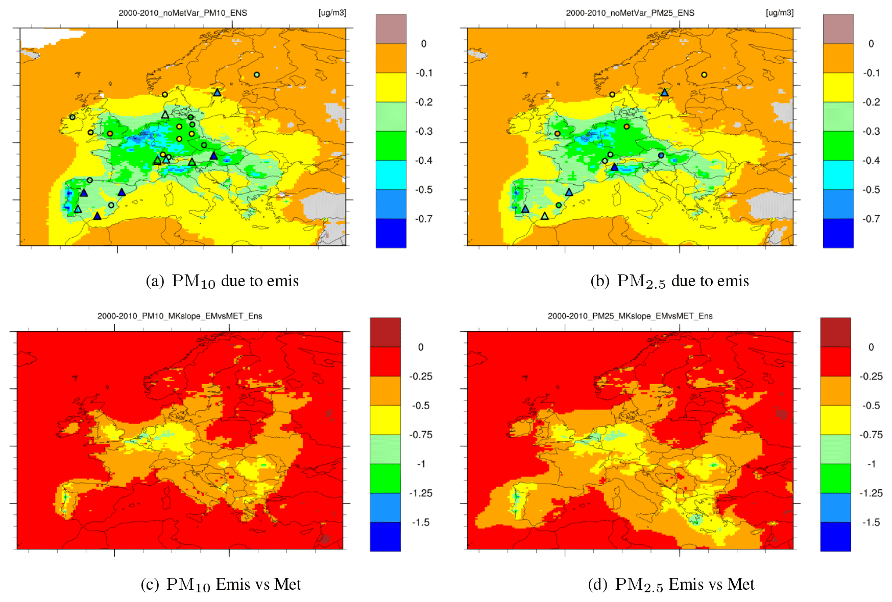
Figure 11PM trends due to emission changes (a, b) and the ratio of PM changes due to emission changes to those due to inter-annual meteorological variability (c, d) for PM10 and PM2.5 in the 2000–2010 period. Observed trends are shown as coloured triangles (significant) and circles (non-significant).
Figure 11 shows that the apparent significance of emission reduction for decreasing PM trends appears to be partially masked by inter-annual meteorological variability in large parts of Europe in the 2000–2010 period. It should be noted that the individual EDT models have different sensitivities to meteorological variability (besides MATCH and LOTO using different meteorological drivers), which may mask the effects of emission changes. The emission reductions play a larger role in PM2.5 trends, as PM10 concentrations (particularly the coarse fraction of natural origin) are more affected by variability in meteorological conditions. Evidently, the most pronounced effects of emission reductions are associated with the regions with greater emission reductions, e.g. Portugal, Benelux, some parts of south-eastern Europe and the Balkan countries. These results are consistent with the main conclusions from the study of PM trends in the period 1998–2007 by Colette et al. (2011). Colette et al. (2017b) arrived at somewhat different conclusions based on a different approach, namely the decomposition of the differences in EDT-modelled PM concentrations in 2000 and 2010 to discriminate the role of emissions, meteorology and boundary conditions. Their analysis suggested a relatively larger average role of emissions compared to the meteorology, though the estimated uncertainties were non-negligible. Due to different premises used by Colette et al. (2017b) and this paper, discrepancies in the outcomes are to be anticipated. That is, here we compared 11-year PM trends to year-to-year PM variability due to meteorological conditions, whereas Colette et al. (2017b) looked at the difference between 2010 and 2000.
To summarize, given rather moderate reductions (and even some increases) in the emissions of some PM precursors and primary PM between 2000 and 2010, we estimate that the effect of emission decreases on 2000–2010 PM trends is roughly of the same order of magnitude as the effect of inter-annual meteorological variability. Separating the effects of emission changes and meteorological variability on PM trends, we get additional insights regarding their relative roles. PM trend slopes due to emission trends (Fig. 11) appear to be quite similar to the total trends wherever the latter are more significant (Fig. 2). The remarkable difference between them is that the trends due to emissions are significant for nearly the entire domain. Model-simulated PM trends due to solely inter-annual meteorological variability (not shown) are by and large very small (±0.05 µg m−3 yr−1) and non-significant everywhere. Thus, our results suggest that the main impact of variable meteorological conditions is to reduce the significance level of PM trends due to emission reductions, while the effects on PM trend slopes are much smaller. For comparison, since the emission reductions during the 1990s were overall larger than in the 2000s, the effect of emission reductions on the decreasing PM trends is estimated to dominate meteorological variability in most of central, eastern and south-eastern Europe (Fig. 11).
The Eurodelta-Trends multi-model experiment, aimed at assessing the efficiency of emission mitigation measures in improving air quality in Europe, was designed to answer a series of questions regarding European pollution trends in the period of 1990–2010. Among these questions are the following. Were there significant trends detected by observations? Do the models manage to reproduce observed trends? How close is the agreement between the models and how large are the deviations from observations? In this paper, we address these issues with respect to PM pollution.
An in-depth trend analysis has been performed for PM10 and PM2.5 for the period of 2000–2010 (limited by the availability of observations), based on results from six CTMs and observational data from the EMEP monitoring network. Given harmonization of set-up and main input data (with a few exceptions), the differences in model results should mainly result from differences in the process formulations within the models themselves, and the spread in the model-simulated trends could be regarded as an indicator of modelling uncertainty.
The results of the analysis strongly indicate overall decreasing trends of annual mean PM10 and PM2.5 concentrations between 2000 and 2010, although the trends are not characterized as significant everywhere. The model-ensemble-simulated mean negative trends vary from below 0.1 µg m−3 yr−1 in northern Europe to 0.1–0.4 µg m−3 yr−1 in the eastern parts and to 0.4–0.7 µg m−3 yr−1 in central Europe and most of the UK, with PM2.5 negative trends being slightly weaker than those for PM10, with the total reductions of annual mean concentrations by between 2 and 5 (7 for PM10) µg m−3 (or between 10 % and 30 %) across most of Europe (by 0.5–2 µg m−3 in Fennoscandia, the north-west of Russia and eastern Europe) during the studied period.
That would mean that the annual mean PM concentrations decreased by between 2 and 5 (7 for PM10) µg m−3 across most of Europe (by 0.5–2 µg m−3 in Fennoscandia, the north-west of Russia and eastern Europe) during the 2000–2010 period. In relative terms, the decrease in annual mean PM10 and PM2.5 was between 10 and 20 % over most of Europe (up to 25 %–30 % in Germany, the Netherlands, Belgium, parts of the UK, Portugal, the north/centre of Italy and large parts of Scandinavia) from 2000 to 2010. We find that the modelled PM trends are fairly consistent with emission reductions in the ECLIPSE_V5 dataset used here. Among possible reasons for deviations between the modelled and observed PM trends are emission uncertainties, impacts of inter-annual variability in meteorological conditions (on pollutant transport and removal, secondary aerosol formation, natural PM emissions, etc.), model uncertainties associated with aerosol formation and removal processes, i.e. SOA formation, cloud pH dependency of SO4 formation, heterogeneous chemistry (including gas–aerosol partitioning of anthropogenic precursors and aerosol formation on base cations of natural origin), SO2 and NH3 co-deposition, etc. Not accounting for forest fires in EDT simulations should also affect the accuracy of simulated PM trends, at least in the regions of large fires, whilst this does not appear to have a major impact on the modelled trends at the EDT sites. Furthermore, we find fairly good general agreement in PM trends estimated by the individual models, with the inter-model variability below 30 %–40 % over much of Europe (up to 50 %–60 % in the northern and eastern parts of the EDT domain). Somewhat greater variability in the modelled PM10 trends reflects larger uncertainties in modelling of the coarse fraction of PM, which is mostly due to natural origin.
Averaged over measurement sites (26 for PM10 and 13 for PM2.5), the mean ensemble-simulated trends are −0.24 µg m−3 yr−1 for PM10 and −0.21 µg m−3 yr−1 for PM2.5, which are somewhat weaker than the observed trends of −0.35 and −0.40 µg m−3 yr−1 respectively. This is partly related to the models' underestimation of PM concentrations. The correspondence between model results and observations appears better in terms of relative trends for the same period, which are −1.7 % yr−1 and −2.0 % yr−1 from the model ensemble and −2.1 % yr−1 and −2.9 % yr−1 from the observations for PM10 and PM2.5 respectively. We see somewhat larger spatial variability of observed PM trends with respect to the modelled trends across Europe and within individual countries, which could partly be explained by the uncertainties associated with national sectoral emissions and their spatial distribution. In addition, the regional models have difficulties in accurately resolving pollution at some of the sites located in the regions with complex topography. The observations identify significant trends for PM10 at 56 % of the sites and for PM2.5 at 36 % of the sites, which is somewhat less than those identified by the models.
The strongest decreasing trends and the largest number of sites (and larger areas) with significant trends were observed and modelled for summer concentrations of PM10 and PM2.5. On the other hand, for the winter season, the model ensemble identifies significant PM trends for very limited areas, mostly in southern parts of Europe, whilst the observed trends are not significant at any of the sites for PM10 and at only 3 out of 14 sites for PM2.5. One important reason for that is the very modest reductions and even increases in the emissions of primary PM from residential heating in winter.
The analysis reveals considerable variability of the role of the individual aerosols in PM10 trends across European countries. The multi-model simulations, supported by available observations, point to decreases in concentrations playing an overall dominant role, although with some exceptions, i.e. we see relatively large contributions of the trends of and to PM10 decreasing trends in Germany, Denmark, Poland and the Po Valley, while the reductions of primary PM emissions appear to be a dominant factor in bringing down PM10 in France, Norway, Portugal, Greece and parts of the UK and Russia.
The analysis also suggests that year-to-year variability in meteorological conditions masks decreasing PM trends due to emission reductions, leading to non-significant trends in many areas and at many monitoring sites between 2000 and 2010. Still, the role of emission reduction measures is pronounced in the regions with greater reductions, where significant trends of PM10 and PM2.5 are both modelled and observed. The EDT model results show that the mean annual trends during the period of 1990–2010 were stronger compared to those in the 2000–2010 period, which is a consequence of larger emission reductions in the 1990s compared to those in the 2000s. The EDT model ensemble estimates that annual mean PM10 and PM2.5 concentrations decreased by between 5 and 15 µg m−3 across most of Europe (by 2–5 µg m−3 in northern Europe) from 1990 to 2021.
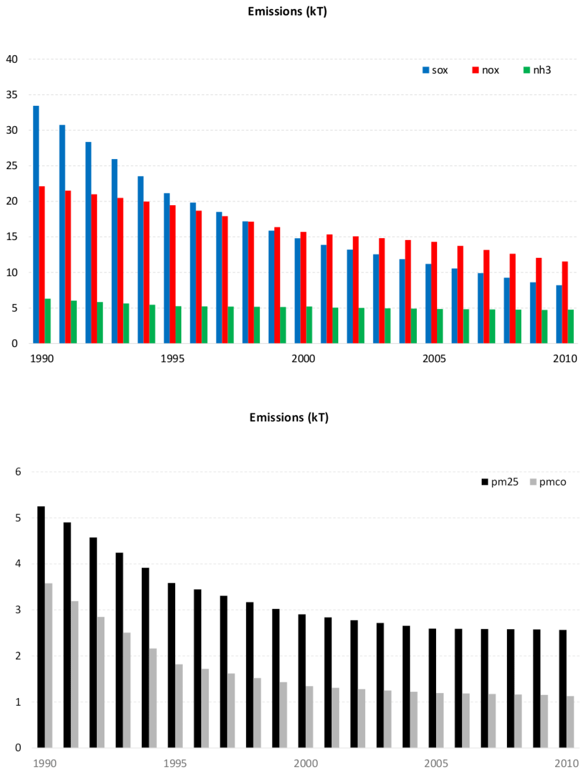
Figure A1Annual emissions of SOx, NOx, NH3, PM2.5 and PM coarse (pmco) in the period 1990–2010 (all countries). Units: ktonnes.
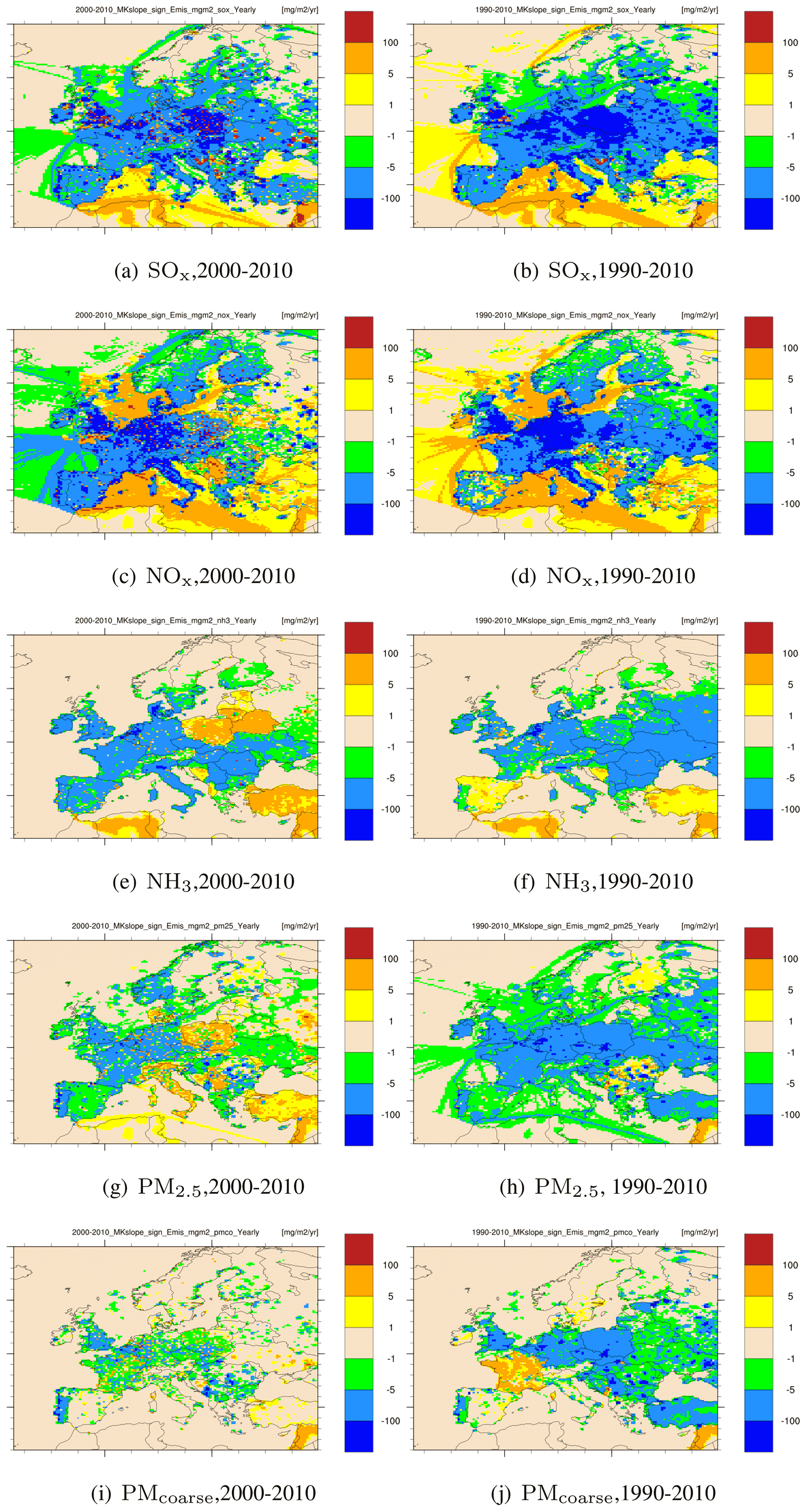
Figure A2Emission trends for 2000–2010 (a, c, e, g, i) and 1990–2010 (b, d, f, h, j).
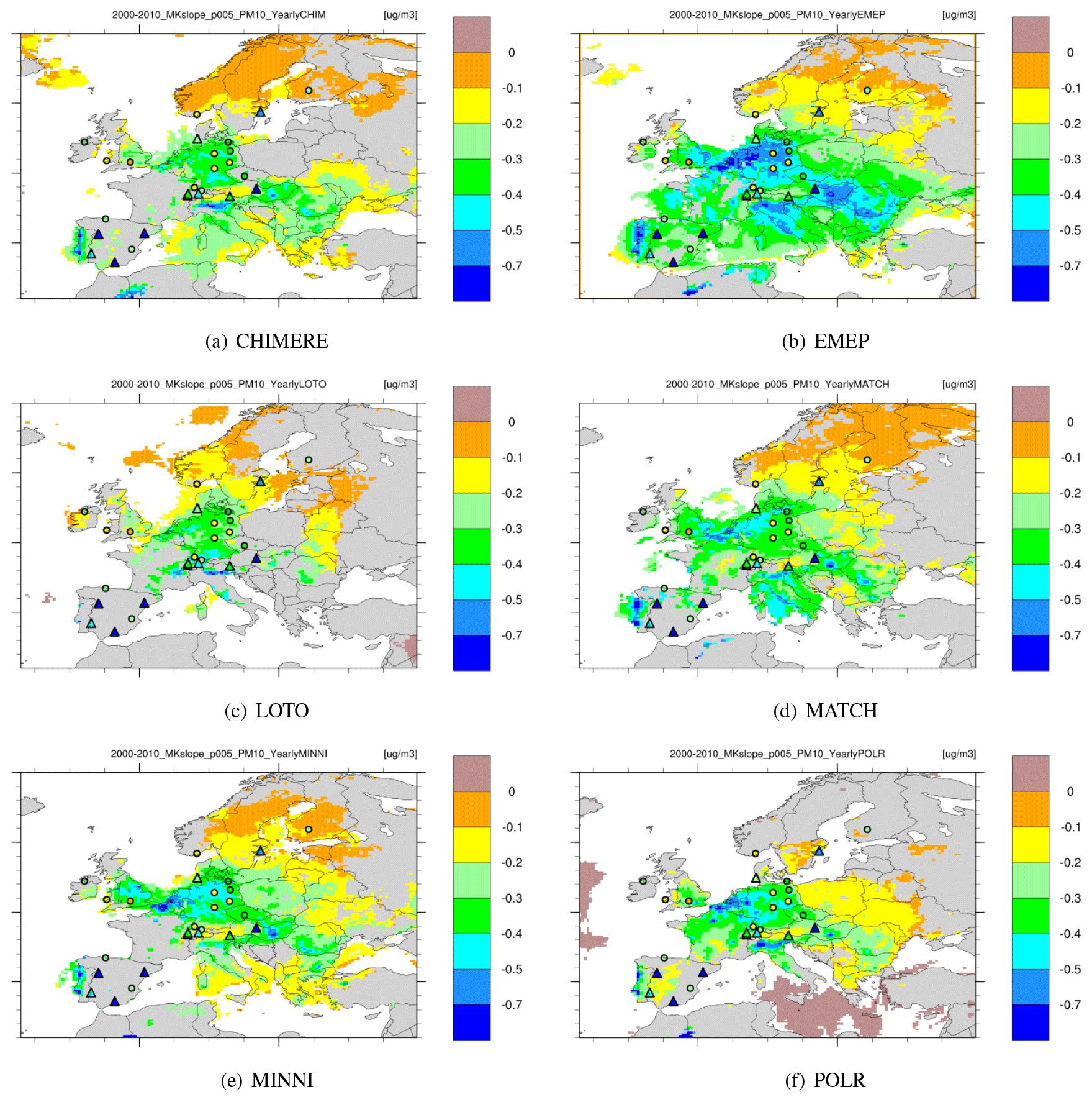
Figure A3Annual mean trends (Sen slopes) for PM10 in the period 2000–2010 as calculated by the individual models. The modelled trends are shown as a coloured contour map (grey or white means non-significant trends) and the observed trends as coloured triangles (significant) and circles (non-significant). Units: µg m−3 yr−1).
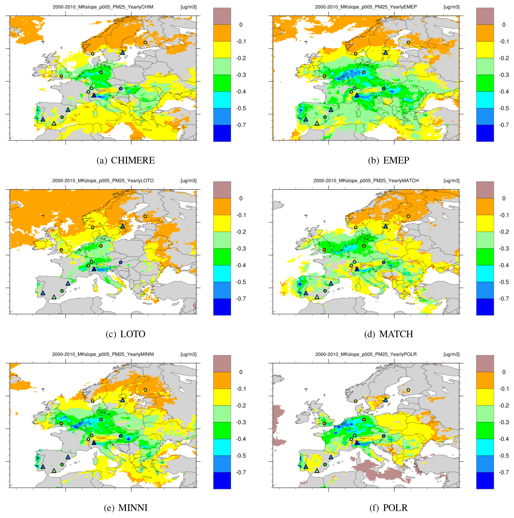
Figure A4Same as Fig. A3 but for PM2.5. Units: µg m−3 yr−1).
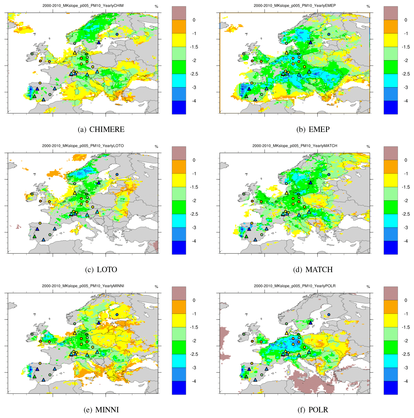
Figure A5Mean Sen slopes relative to the starting year of 2000 (% yr−1) for PM10 trends in the period 2000–2010 calculated by the individual models. The modelled trends are shown as a coloured contour map (grey or white means non-significant trends) and the observed trends as coloured triangles (significant) and circles (non-significant).
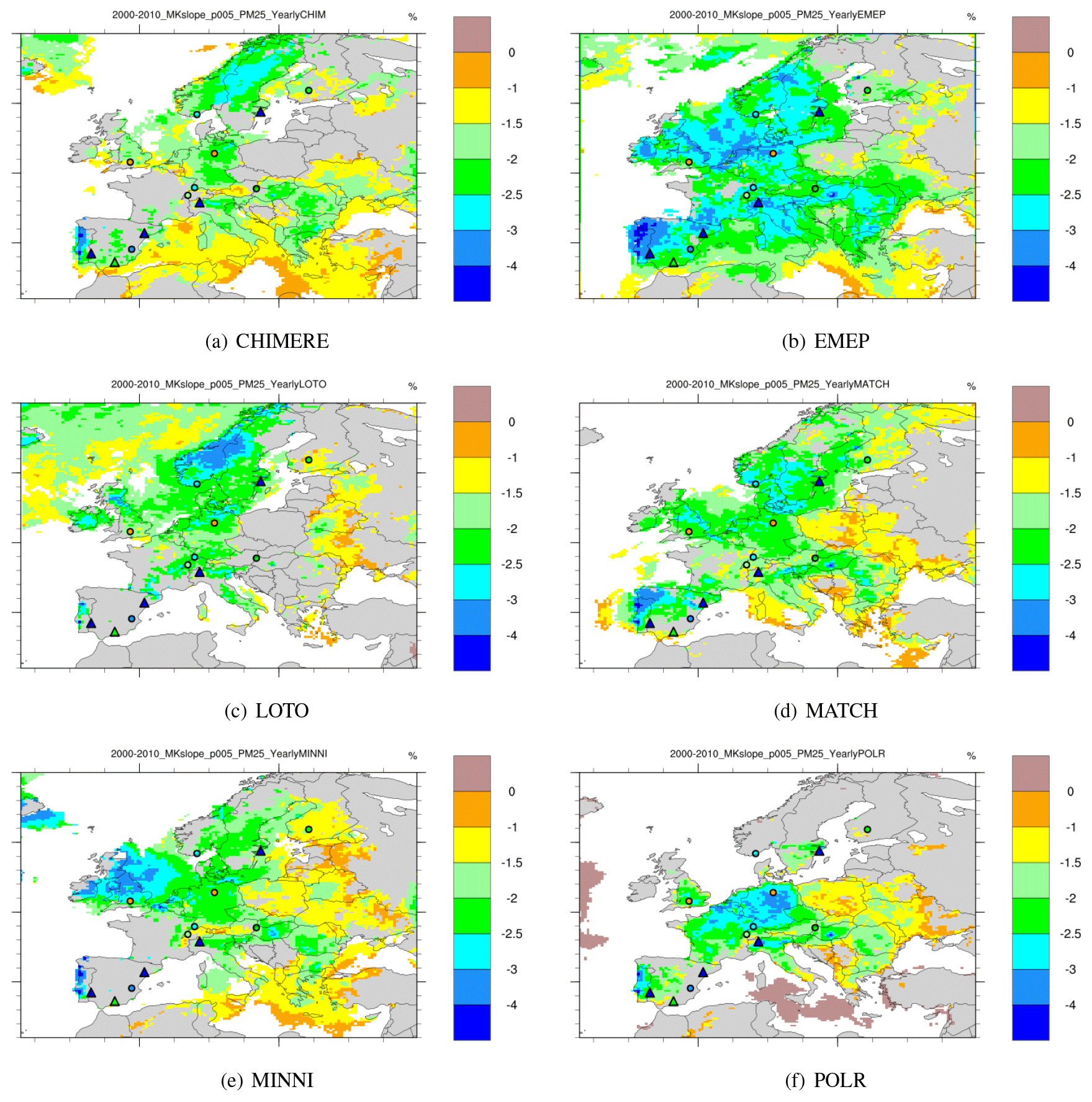
Figure A6Same as Fig. A5 but for PM2.5. Units: % yr−1.
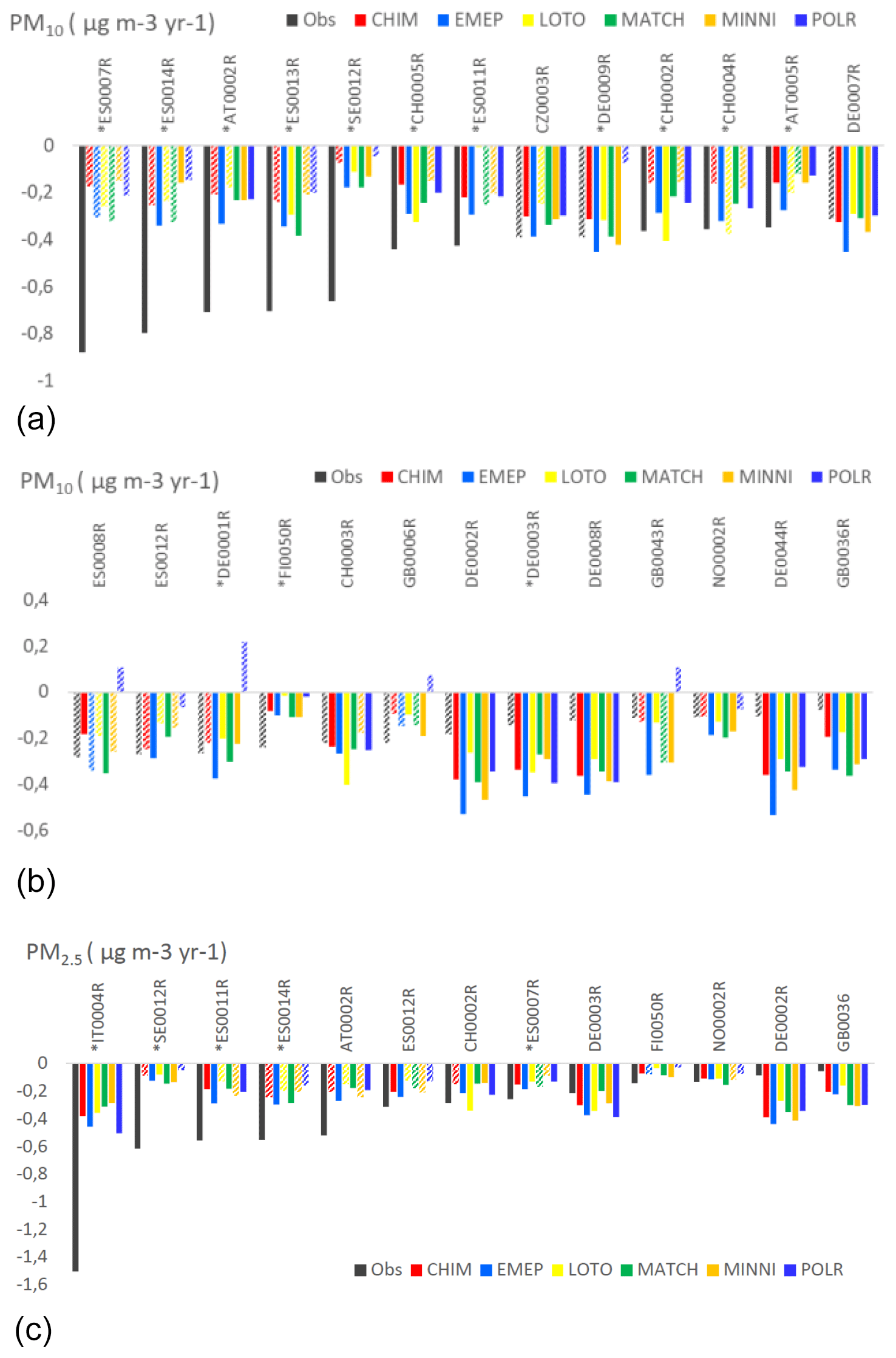
Figure A7Observed and modelled trend slopes (µg m−3 yr−1) for the period 2000–2010 at the trend sites for PM10 (a, b) and for PM2.5 (c). The sites are sorted by decreasing observed negative trends; insignificant trends are shown as striped bars. Units: µg m−3 yr−1.
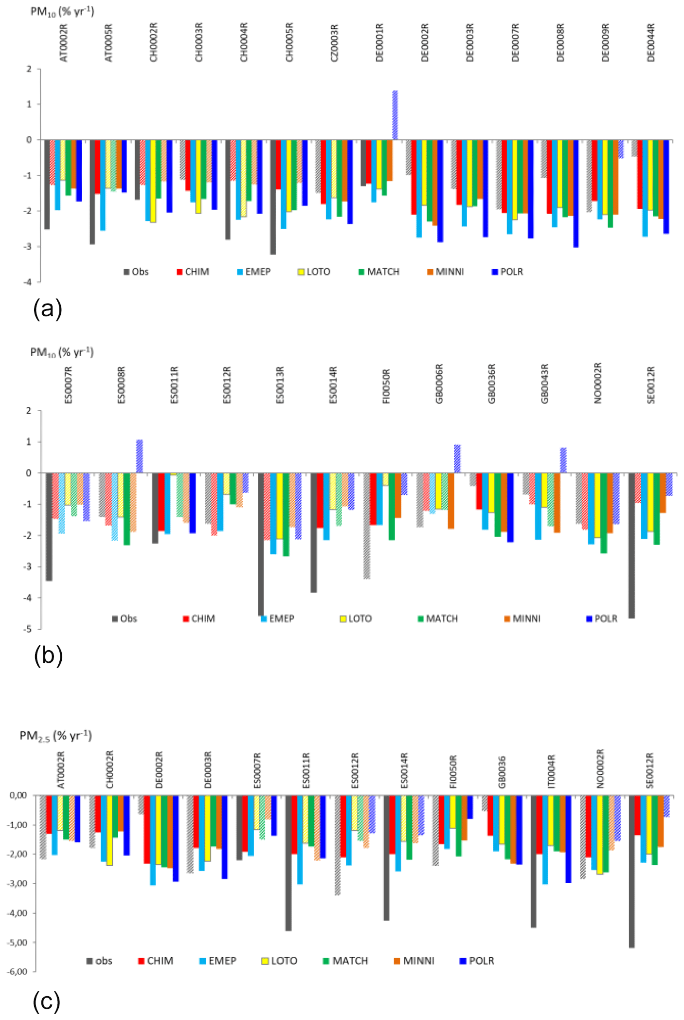
Figure A8Mean observed (black) and modelled (coloured) relative trends for PM10 (a, b) and PM2.5 (c) in the period 2000–2010 at the individual trend sites. Insignificant modelled trends are shown as striped bars. Units: % yr−1.
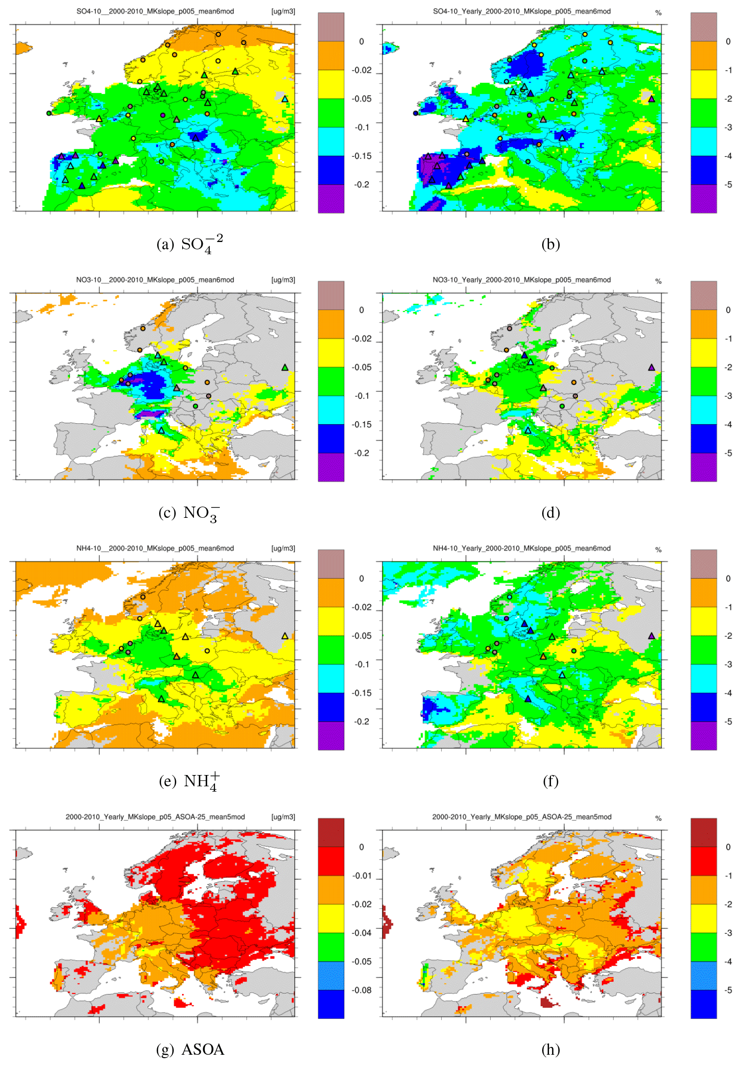
Figure A9Mean Sen trend slopes, observed and from six-model ensemble, for 2000–2010 for anthropogenic aerosols , and (a–f) and simulated with the five-model ensemble for ASOA (note the different colour scale). (a, c, e, g) Absolute (µg m−3 yr−1) and (b, d, f, h) panels – relative (% yr−1) trends. The modelled trends are shown as the coloured contour map (grey or white means non-significant trends) and the observed trends as coloured triangles (significant) and circles (non-significant).
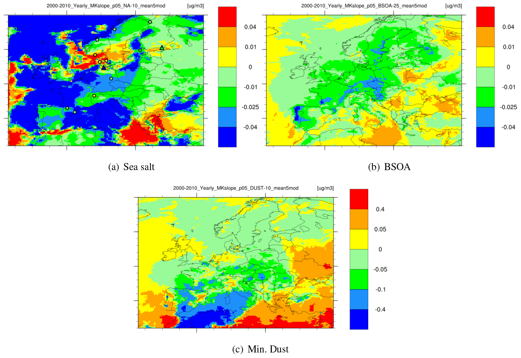
Figure A10Mean Sen trend slopes for 2000–2010 simulated by the six-model ensemble for natural aerosols: (a) sea salt (observed trends also shown); (b) BSOA and (c) mineral dust. The modelled trends are shown as the coloured contour map (grey or white means non-significant trends) and the observed trends as coloured triangles (significant) and circles (non-significant).
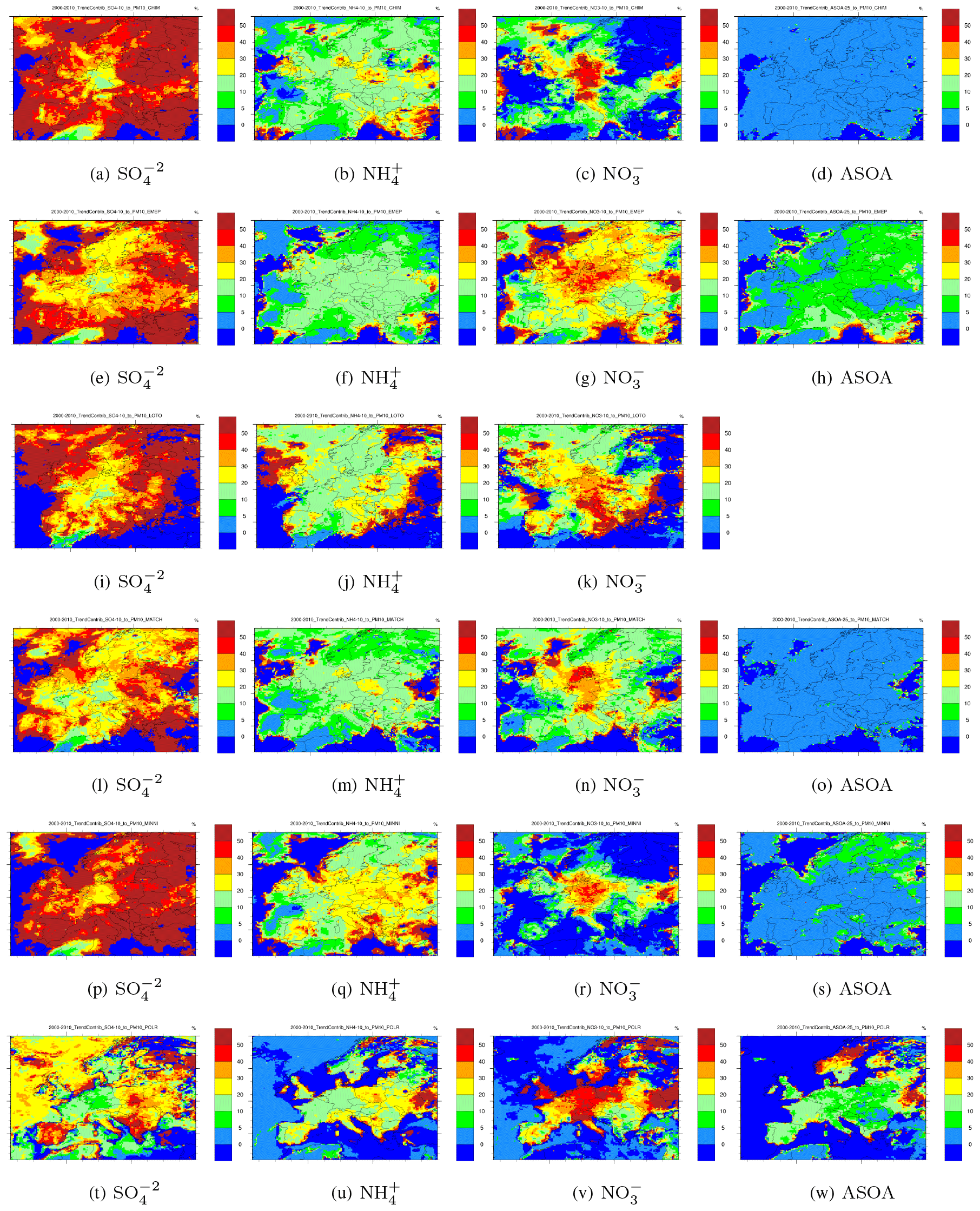
Figure A11Relative contributions of (from left to right) , , and ASOA to PM10 trends between 2000 and 2010 calculated by (from top to bottom) the CHIMERE, EMEP, LOTOS-EUROS, MATCH, MINNI and Polair3D models.
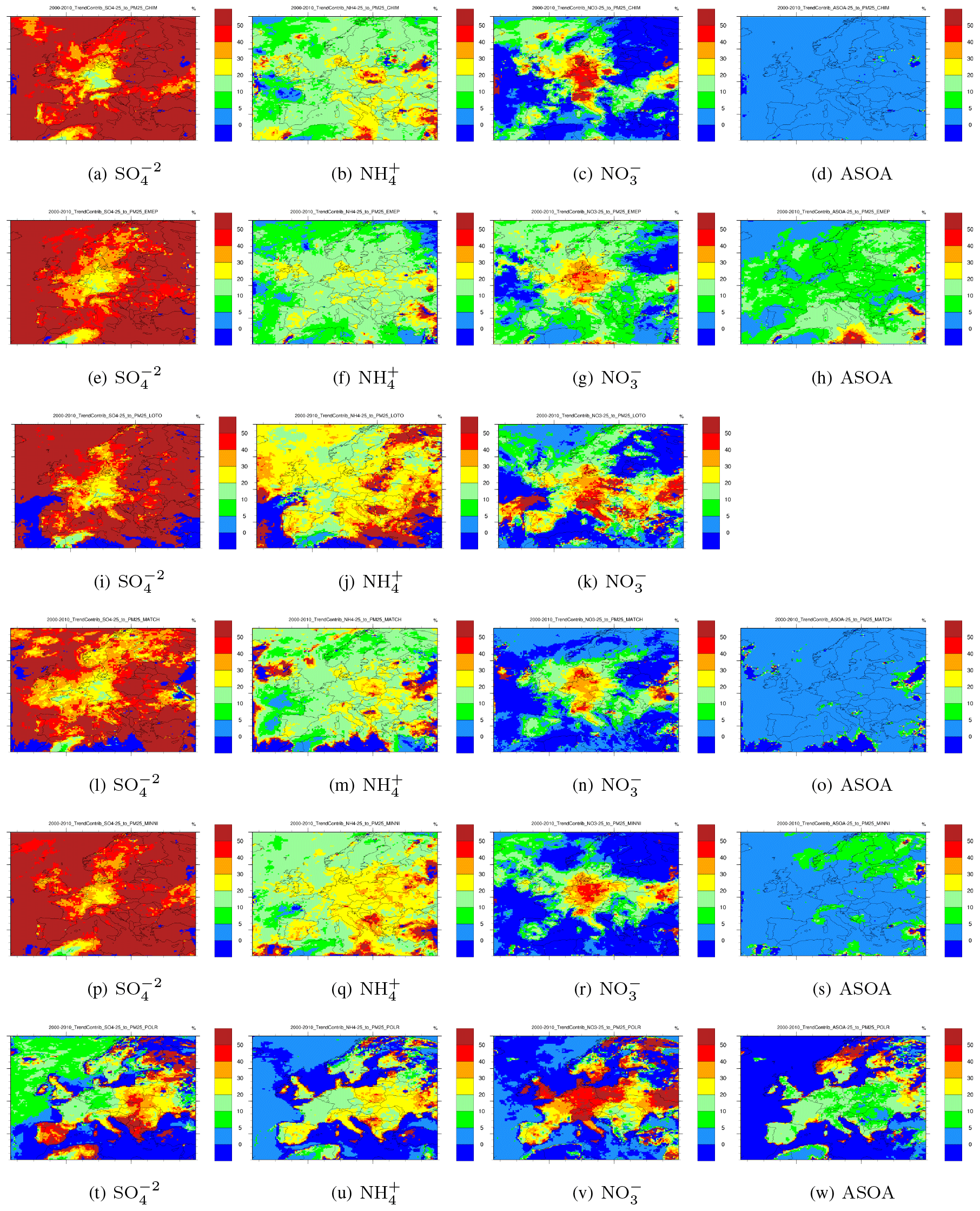
Figure A12Relative contributions of (from left to right) , , and ASOA to PM2.5 trends between 2000 and 2010 calculated by (from top to bottom) the CHIMERE, EMEP, LOTOS-EUROS, MATCH, MINNI and Polair3D models.
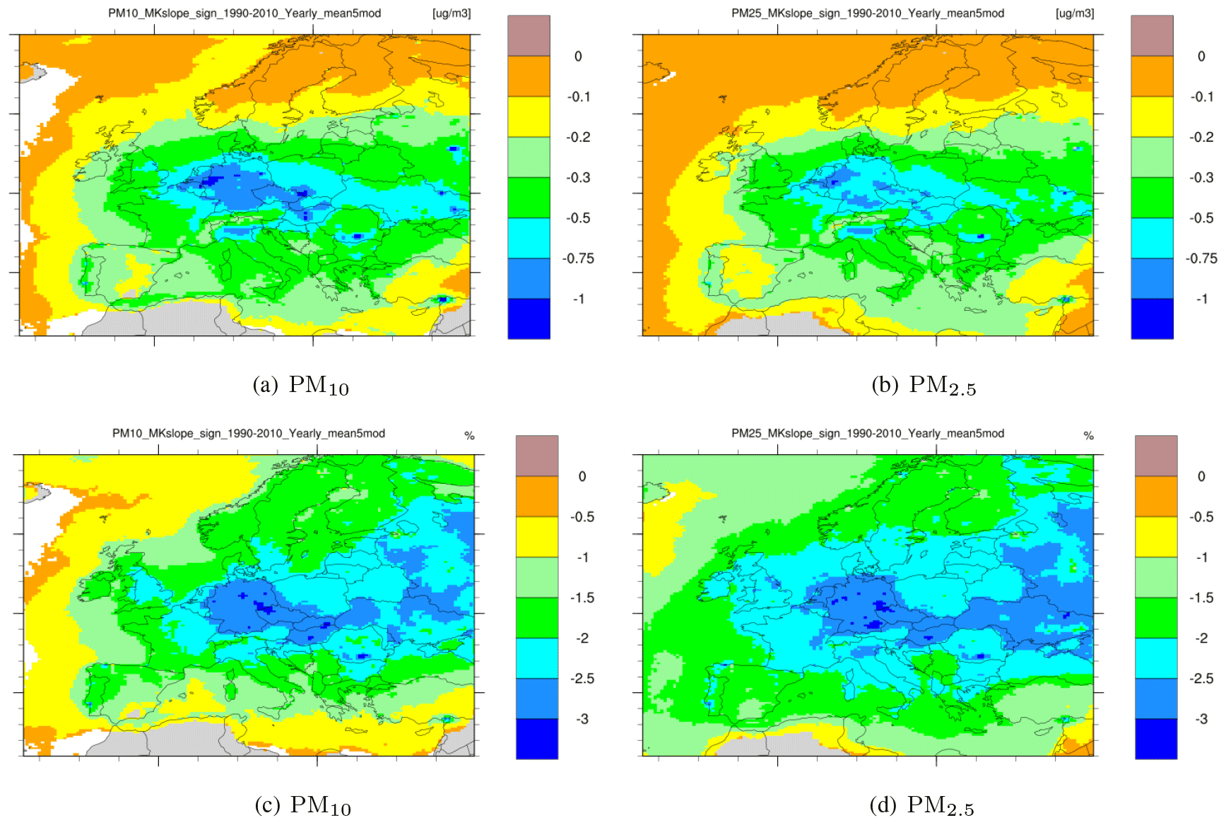
Figure A13Annual mean Sen slope for trends in the period 1990–2010 as calculated by the six-model ensemble (a, c) for PM10 and (b, d) PM2.5. Upper panels – absolute (µg m−3 yr−1) – and lower panels – relative to 1990 (% yr−1).
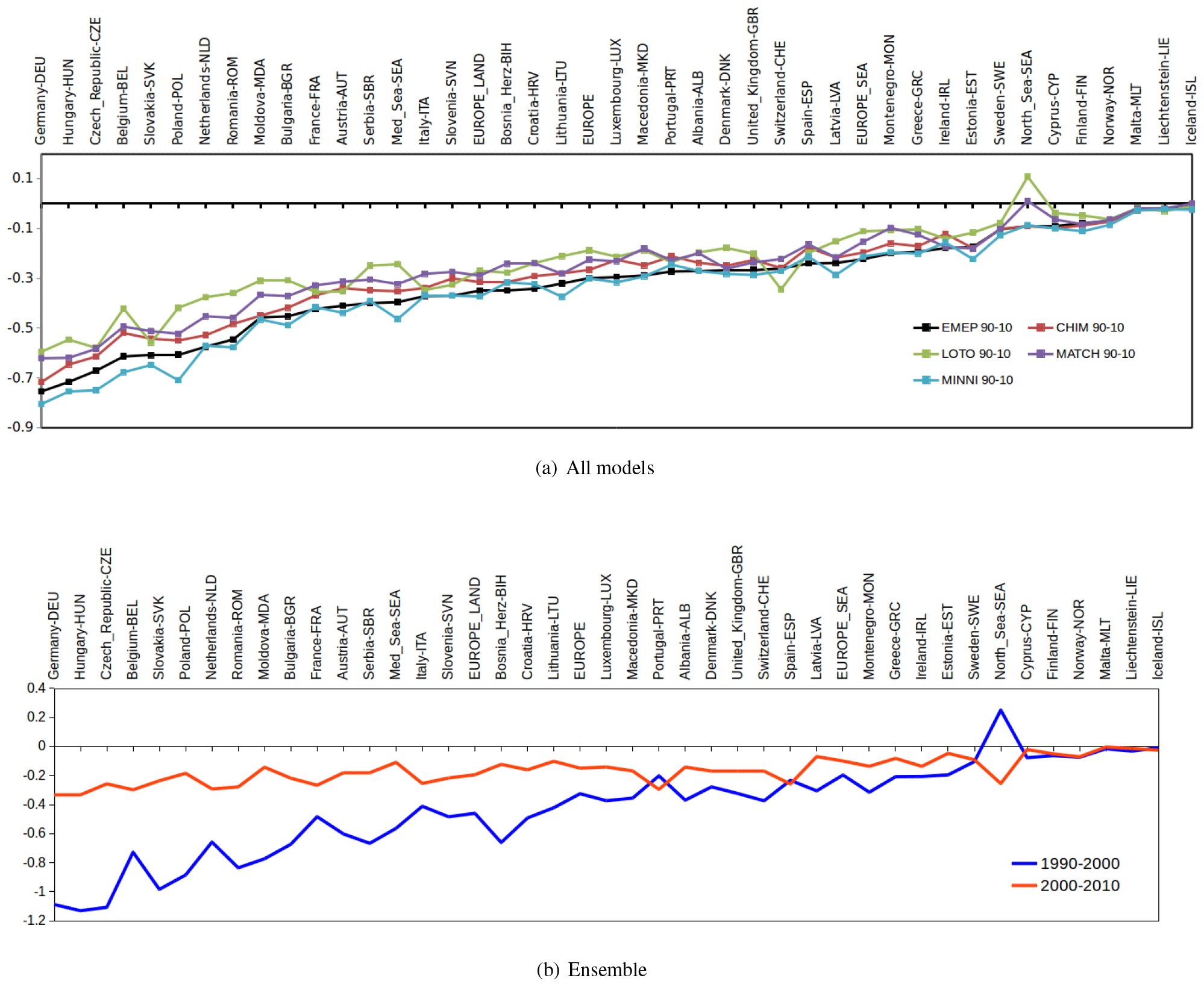
Figure A14Modelled PM10 trends calculated for European countries (µg m−3 yr−1): (a) the individual models for the period 1990–2010 and (b) the model ensemble for the periods 1990–2000 and 2000–2010 separately. The countries are ranged according to descending 1990–2010 negative trends from the EMEP model (a).
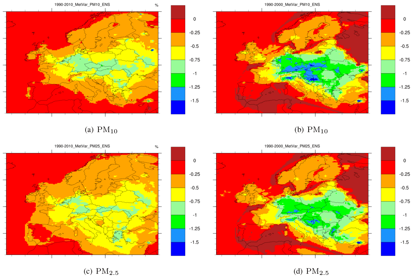
Figure A15The ratio of PM changes due to emission changes to those due to inter-annual meteorological variability for PM10 and PM2.5 for the 1990–2010 (a, c) and 1990–2000 (b, d) periods.
Table A1Selected set of EMEP monitoring stations for PM10 and PM2.5 trend analysis for the period 2000–2010.
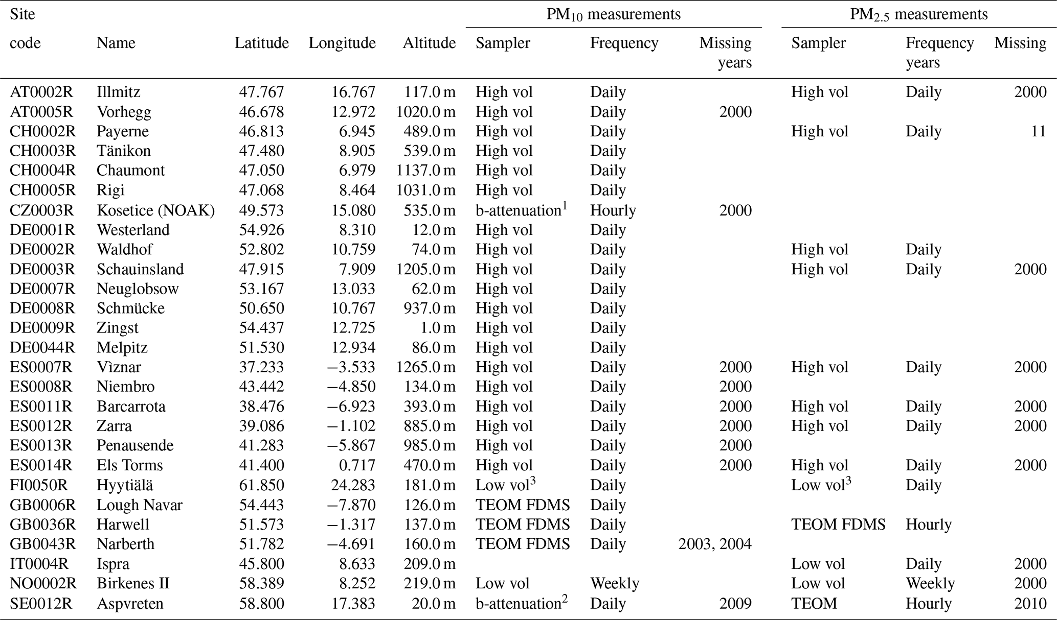
Table A2Relative bias (%) and correlation (R) for modelled PM10 with respect to available observations at 26 EDT sites for the years 2000 to 2010.

Bias – relative bias (%); * excluding coarse sea salt.
Table A3Relative bias (%) and correlation (R) for modelled PM2.5 with respect to available observations at 13 EDT sites for the years 2000 to 2010.
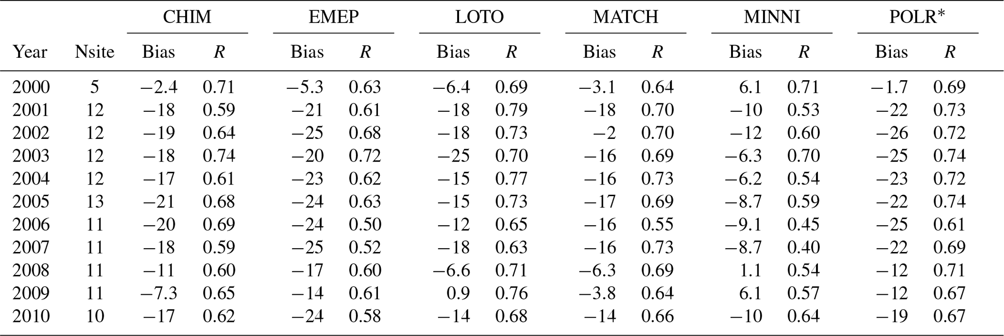
Bias – relative bias expressed (%).
Table A4Brief description of the CTMs involved in the Eurodelta-Trends modelling exercise (extended version of Table S1 in the Supplement to Colette et al., 2017a).
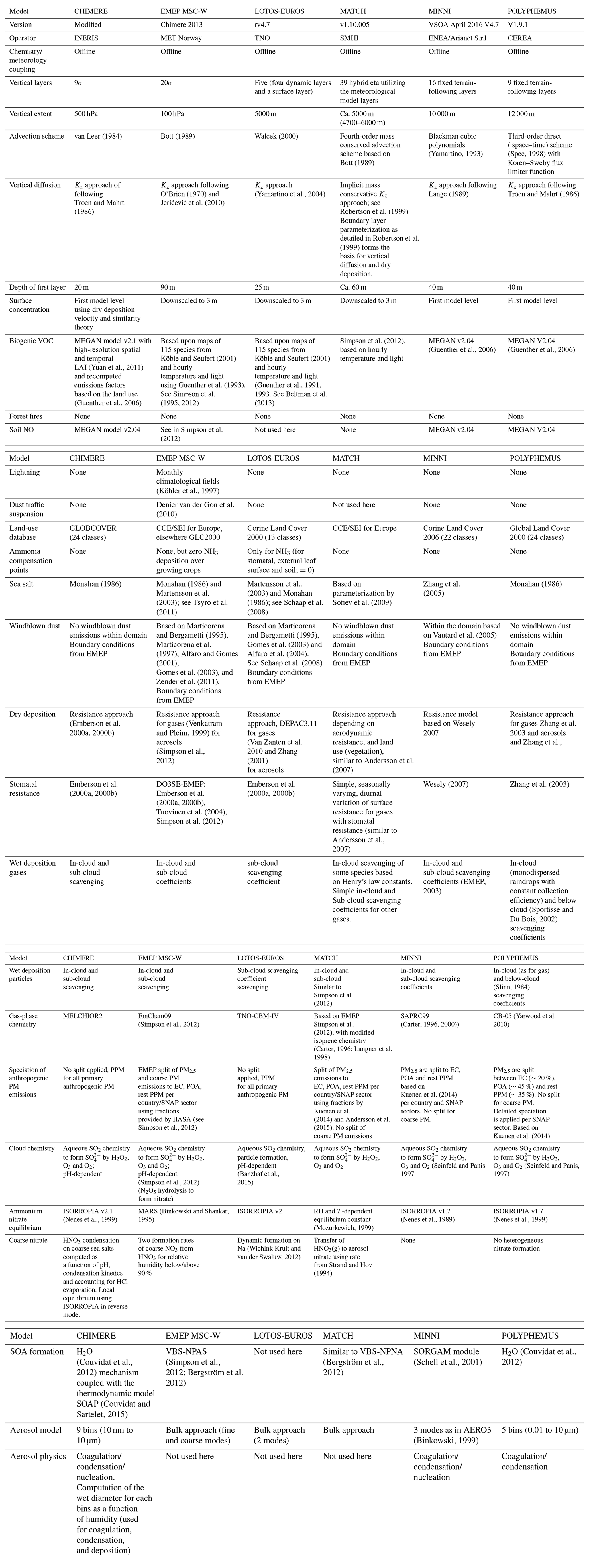
* EC: elemental carbon. POA: primary organic aerosol. ASOA and BSOA: anthropogenic and biogenic secondary aerosol. TPPM: total primary PM (EC + POA + remaining PPM).
Technical details of the Eurodelta project simulations that permit the replication of the experiment are available on the wiki of the EMEP Task Force on Measurement and Modelling (https://wiki.met.no/emep/emep-experts/tfmmtrendeurodelta; TFMM/EMEP, 2015), which also includes ESGF links to corresponding input forcing data. The Eurodelta-Trends model results are made available for public use on the AeroCom server (information to gain access to the AeroCom server is available at https://aerocom.met.no/FAQ/data_access; AeroCom, 2018). Model input and output data are permanently stored in the /metno/aerocom-users-database/EURODELTA folder on the AeroCom server. See Colette et al. (2017) for full terms and conditions for the use of these data. The original data used for calculating aggregated concentrations are all available from the EBAS database infrastructure (https://ebas.nilu.no; NILU, 2017).
ACo coordinated the Eurodelta-Trends (EDT) exercise and WA was responsible for the compilation and quality control of the observations. The following modelling teams set up, pre-processed, ran and post-processed the simulations for each model: FC, BB, MGV and ACo for CHIM; ST and PW for EMEP; AM and MS for LOTO; CA and RB for MATCH; MM, MA, GB, ACa and MD for MINNI; YR and VR for POLR. WA and CK contributed with production of figures. Additional post-processing of model output and uploading to the AeroCom server were done by KC. All of the analyses presented in this paper were carried out by ST, assisted by discussions with WA and HF and with valuable contributions from ACo, CA, AM, GC, YR, BB, MT, MGV, NO, KM, FC and MTP. Special thanks for language proofreading go to MT.
The contact author has declared that neither they nor their co-authors have any competing interests.
Publisher's note: Copernicus Publications remains neutral with regard to jurisdictional claims in published maps and institutional affiliations.
Computer time for the EMEP model runs was supported by the Research Council of Norway through the NOTUR project EMEP (NN2890K), for CPU, and the NorStore project European Monitoring and Evaluation Programme (NS9005K), for the storage of data. LOTOS-team thanks Erik van Meijgaard of the Royal Netherlands Meteorological Institute (KNMI), for providing the RACMO2 simulations that were used by LOTOS-EUROS. The computing resources and the related technical support used for the MINNI simulations have been provided by CRESCO/ENEAGRID High Performance Computing infrastructure and its staff. The infrastructure is funded by ENEA, the Italian National Agency for New Technologies, Energy and Sustainable Economic Development and by Italian and European research programmes (http://www.cresco.enea. it/english, last access: 21 December 2018). The GAINS emission trends used in this work were produced as part of the FP7 European Research Project ECLIPSE (Evaluating the Climate and Air Quality Impacts of Short-Lived Pollutants; grant no. 282688). Meteorological forcing with the WRF model was provided by Robert Vautard and Annemiek Stegehuis from LSCE/IPSL.
The Ineris coordination of the EURODELTA-Trends exercise has been supported by the French Ministry in charge of Ecology in the context of the Task Force on Measurement and Modelling of the EMEP program of the LRTAP Convention. The CHIMERE simulations were performed using the TGCC supercomputers under GENCI computing allocation. The work of EMEP MSC-W has been supported by the EMEP Trust Fund under the United Nations Economic Commission for Europe (UN ECE). Funding for the MATCH participation was jointly divided between Nordforsk through the research programme Nordic Welfare (grant no. 75007), the Swedish Environmental Protection Agency through the SCAC research programme, and the 2017–2018 Belmont Forum and BiodivERsA joint call for research proposals, under the BiodivScen ERA-Net COFUND programme, with the funding organisations AKA (contract no. 326328), ANR (grant no. ANR-18-EBI4-007), BMBF (KFZ; grant no. 01LC1810A), FORMAS (contract nos. 2018-02434, 2018-02436, 2018-02437, and 2018-02438) and MICINN (APCIN; grant no. PCI2018-093149). Giancarlo Ciarelli has been supported by ADEME and the Swiss National Science Foundation (grant no. P2EZP2_175166). MINNI participation in this project was supported by the “Cooperation Agreement for support to international Conventions, Protocols and related negotiations on air pollution issues”, funded by the Italian Ministry for the Environment, Land and Sea. Financial support for the Institute for Advanced Sustainability Studies (IASS) has been provided by the Federal Ministry of Education and Research of Germany (BMBF) and the Ministry for Science, Research and Culture of the State of Brandenburg (MWFK). The work of CIEMAT has been supported by the Ministry for the Ecological Transition and Demographic Challenge (MITERD).
This paper was edited by Stefano Galmarini and reviewed by Paul A. Makar and one anonymous referee.
Aas, W., Mortier, A., Bowersox, V., Cherian, R., Faluvegi, G., Fagerli, H., Hand, J., Klimont, Z., Galy-Lacaux, C., Lehmann, C. M., Myhre, C. L., Myhre, G., Olivié, D., Sato, K., Quaas, J., Rao, P. S. P., Schulz, M., Shindell, D., Skeie, R. B., Stein, A., Takemura, T., Tsyro, S., Vet, R., and Xu, X.: Global and regional trends of atmospheric sulfur, Scient. Rep., 9, 1–11, https://doi.org/10.1038/s41598-018-37304-0., 2019. a
Aas, W., Fagerli, H., Yttri, K. E., Tsyro, S., Solberg, S., Simpson, D., Gliß, J., Mortier, A., Grøtting Wærsted, E., Brenna, H., Hjellbrekke, A., Griesfeller, J., Nyíri, A., Gauss, M., and Scheuschner, T.: Trends in observations and EMEP MSC-W model calculations 2000–2019, in: Transboundary particulate matter, photo-oxidants, acidifying and eutrophying components, EMEP Status Report 1/2021, The Norwegian Meteorological Institute, Oslo, Norway, 83–97, https://emep.int/publ/reports/2021/EMEP_Status_Report_1_2021.pdf, last access: 3 September 2021. a
AeroCom: How to retrieve data from AeroCom server, https://aerocom.met.no/FAQ/data_access (last access: 6 January 2022), 2018. a
Alfaro, S. C. and Gomes, L.: Modeling mineral aerosol production by wind erosion: Emission intensities and aerosol size distributions in source areas, J. Geophys. Res.-Atmos., 106, 18075–18084, https://doi.org/10.1029/2000JD900339, 2001. a, b
Alfaro, S. C., Rajot, J. L., and Nickling, W.: Estimation of PM20 emissions by wind erosion: main sources of uncertainties, Geomorphology, 59, 63–74, https://doi.org/10.1016/j.geomorph.2003.09.006, 2004. a
Amann, M.: Future emissions of air pollutants in Europe-Current legislation baseline and the scope for further reductions, http://pure.iiasa.ac.at/id/eprint/10164/1/XO-12-011.pdf (last access: 2 June 2022), 2012. a
Amann, M., Bertok, I., Borken-Kleefeld, J., Cofala, J., Heyes, C., Höglund-Isaksson, L., Klimont, Z., Nguyen, B., Posch, M., Rafaj, P., Sandler, R., Schöpp, W., Wagner, F., and Winiwarter, W.: Cost-effective control of air quality and greenhouse gases in Europe: Modeling and policy applications, Environ. Model. Softw., 26, 1489–1501, 2011. a, b
Andersson, C., Langner, J., and Bergström, R.: Interannual variation and trends in air pollution over Europe due to climate variability during 1958–2001 simulated with a regional CTM coupled to the ERA40 reanalysis, Tellus B, 59, 77–98, https://doi.org/10.1111/j.1600-0889.2006.00231.x, 2007. a, b, c, d
Andersson, C., Bergström, R., Bennet, C., Robertson, L., Thomas, M., Korhonen, H., Lehtinen, K., and Kokkola, H.: MATCH-SALSA – Multi-scale Atmospheric Transport and CHemistry model coupled to the SALSA aerosol microphysics model – Part 1: Model description and evaluation, Geosci. Model Dev., 8, 171–189, https://doi.org/10.5194/gmd-8-171-2015, 2015. a, b
Banzhaf, S., Schaap, M., Kranenburg, R., Manders, A. M. M., Segers, A. J., Visschedijk, A. J. H., Denier van der Gon, H. A. C., Kuenen, J. J. P., van Meijgaard, E., van Ulft, L. H., Cofala, J., and Builtjes, P. J. H.: Dynamic model evaluation for secondary inorganic aerosol and its precursors over Europe between 1990 and 2009, Geosci. Model Dev., 8, 1047–1070, https://doi.org/10.5194/gmd-8-1047-2015, 2015. a, b
Barmpadimos, I., Keller, J., Oderbolz, D., Hueglin, C., and Prévôt, A. S. H.: One decade of parallel fine (PM2.5) and coarse (PM10–PM2.5) particulate matter measurements in Europe: trends and variability, Atmospheric Chemistry and Physics, 12, 3189–3203, https://doi.org/10.5194/acp-12-3189-2012, 2012. a
Beltman, J. B., Hendriks, C., Tum, M., and Schaap, M.: The impact of large scale biomass production on ozone air pollution in Europe, Atmos. Environ., 71, 352–363, https://doi.org/10.1016/j.atmosenv.2013.02.019, 2013. a, b
Bergström, R., Denier Van Der Gon, H., Prévôt, A. S., Yttri, K. E., and Simpson, D.: Modelling of organic aerosols over Europe (2002–2007) using a volatility basis set (VBS) framework: application of different assumptions regarding the formation of secondary organic aerosol, Atmos. Chem. Phys., 12, 8499–8527, https://doi.org/10.5194/acp-12-8499-2012, 2012. a, b, c, d
Bergström, R., Hallquist, M., Simpson, D., Wildt, J., and Mentel, T. F.: Biotic stress: a significant contributor to organic aerosol in Europe?, Atmos. Chem. Phys., 14, 13643–13660, https://doi.org/10.5194/acp-14-13643-2014, 2014. a
Bessagnet, B., Pirovano, G., Mircea, M., Cuvelier, C., Aulinger, A., Calori, G., Ciarelli, G., Manders, A., Stern, R., Tsyro, S., García Vivanco, M., Thunis, P., Pay, M.-T., Colette, A., Couvidat, F., Meleux, F., Rouïl, L., Ung, A., Aksoyoglu, S., Baldasano, J. M., Bieser, J., Briganti, G., Cappelletti, A., D'Isidoro, M., Finardi, S., Kranenburg, R., Silibello, C., Carnevale, C., Aas, W., Dupont, J.-C., Fagerli, H., Gonzalez, L., Menut, L., Prévôt, A. S. H., Roberts, P., and White, L.: Presentation of the EURODELTA III intercomparison exercise – evaluation of the chemistry transport models' performance on criteria pollutants and joint analysis with meteorology, Atmos. Chem. Phys., 16, 12667–12701, https://doi.org/10.5194/acp-16-12667-2016, 2016. a
Bieser, J., Aulinger, A., Matthias, V., Quante, M., and Van Der Gon, H. D.: Vertical emission profiles for Europe based on plume rise calculations, Environ. Pollut., 159, 2935–2946, 2011. a
Binkowski, F. S.: Aerosols in models-3 CMAQ, Science algorithms of the EPA Models-3 Community multiscale air quality (CMAQ) modeling system, https://cfpub.epa.gov/si/si_public_file_download.cfm?p_download_id=524687 (last access: 30 May 2022), 1999. a
Binkowski, F. S. and Shankar, U.: The regional particulate matter model: 1. Model description and preliminary results, J. Geophys. Res.-Atmos., 100, 26191–26209, https://doi.org/10.1029/95JD02093, 1995. a, b
Bott, A.: A positive definite advection scheme obtained by nonlinear renormalization of the advective fluxes, Mon. Weather Rev., 117, 1006–1016, 1989. a, b
Carter, W. P.: Condensed atmospheric photooxidation mechanisms for isoprene, Atmos. Environ., 30, 4275–4290, https://doi.org/10.1016/1352-2310(96)00088-X, 1996. a, b
Carter, W. P.: Documentation of the SAPRC-99 chemical mechanism for VOC reactivity assessment, Contract, 92, 95–308, https://intra.engr.ucr.edu/~carter/pubs/s99doc.pdf (last access: 30 May 2022), 2000. a
Ciarelli, G., Theobald, M. R., Vivanco, M. G., Beekmann, M., Aas, W., Andersson, C., Bergström, R., Manders-Groot, A., Couvidat, F., Mircea, M., Tsyro, S., Fagerli, H., Mar, K., Raffort, V., Roustan, Y., Pay, M.-T., Schaap, M., Kranenburg, R., Adani, M., Briganti, G., Cappelletti, A., D'Isidoro, M., Cuvelier, C., Cholakian, A., Bessagnet, B., Wind, P., and Colette, A.: Trends of inorganic and organic aerosols and precursor gases in Europe: insights from the EURODELTA multi-model experiment over the 1990–2010 period, Geosci. Model Dev., 12, 4923–4954, https://doi.org/10.5194/gmd-12-4923-2019, 2019. a, b, c, d, e
Colette, A., Granier, C., Hodnebrog, Ø., Jacobs, H., Maurizi, A., Nyíri, A., Bessagnet, B., D'Angiola, A., D'Isidoro, M., Gauss, M., Meleux, F., Memmesheimer, M., Mieville, A., Rouïl, L., Russo, F., Solberg, S., Stordal, F., and Tampieri, F.: Air quality trends in Europe over the past decade: a first multi-model assessment, Atmos. Chem. Phys., 11, 11657–11678, https://doi.org/10.5194/acp-11-11657-2011, 2011. a, b, c
Colette, A., Aas, W., Banin, L., Braban, C., Ferm, M., González Ortiz, A., Ilyin, I., Mar, K., Pandolfi, M., Putaud, J.-P., Shatalov, V., Solberg, S., Spindler, G., Tarasova, O., Vana, M., Adani, M., Almodovar, P., Berton, E., Bessagnet, B., Bohlin-Nizzetto, P., Boruvkova, J., Breivik, K., Briganti, G., Cappelletti, A., Cuvelier, K., Derwent, R., D'Isidoro, M., Fagerli, H., Funk, C., Garcia Vivanco, M., González Ortiz, A., Haeuber, R., Hueglin, C., Jenkins, S., Kerr, J., de Leeuw, F., Lynch, J., Manders, A., Mircea, M., Pay, M., Pritula, D., Putaud, J.-P., Querol, X., Raffort, V., Reiss, I., Roustan, Y., Sauvage, S., Scavo, K., Simpson, D., Smith, R., Tang, Y., Theobald, M., Tørseth, K., Tsyro, S., van Pul, A., Vidic, S., Wallasch, M., and Wind, P.: Air Pollution trends in the EMEP region between 1990 and 2012, Tech. Rep. Joint Report of the EMEP Task Force on Measurements and Modelling (TFMM), Chemical Co-ordinating Centre (CCC), Meteorological Synthesizing Centre-East (MSC-E), Meteorological Synthesizing Centre-West (MSC-W) EMEP/CCC Report 1/2016, Norwegian Institute for Air Research, Kjeller, Norway, http://www.unece.org/fileadmin/DAM/env/documents/2016/AIR/Publications/Air_pollution_trends_in_the_EMEP_region.pdf (last access: 2 June 2022), 2016. a, b, c, d, e
Colette, A., Andersson, C., Manders, A., Mar, K., Mircea, M., Pay, M.-T., Raffort, V., Tsyro, S., Cuvelier, C., Adani, M., Bessagnet, B., Bergström, R., Briganti, G., Butler, T., Cappelletti, A., Couvidat, F., D'Isidoro, M., Doumbia, T., Fagerli, H., Granier, C., Heyes, C., Klimont, Z., Ojha, N., Otero, N., Schaap, M., Sindelarova, K., Stegehuis, A. I., Roustan, Y., Vautard, R., van Meijgaard, E., Vivanco, M. G., and Wind, P.: EURODELTA-Trends, a multi-model experiment of air quality hindcast in Europe over 1990–2010, Geosci. Model Dev., 10, 3255–3276, https://doi.org/10.5194/gmd-10-3255-2017, 2017a. a, b, c, d, e, f, g
Colette, A., Solberg, S., Beauchamp, M., Bessagnet, B., Malherbe, L., Guerreiro, C., and Team, E.-T. M.: Long term air quality trends in Europe. Contribution of meteorological variability, natural factors and emissions, Long term air quality trends in EuropeContribution of meteorological variability, natural factors and emissions, ETC/ACM Technical Paper 2016/7, ETC/A – European Topic Centre on Air Pollution and Climate Change Mitigation,Bilthoven, the Netherlands, https://www.eionet.europa.eu/etcs/etc-atni/products/etc-atni-reports/etcacm_tp_2016_7_aqtrendseurope (last access: 2 June 2022), 2017b. a, b, c
Colette, A., Solberg, S., Aas, W., and Walker, S.-E.: Understanding Air Quality Trends in Europe, Eionet Report – ETC/ATNI 2020/8, https://www.eionet.europa.eu/etcs/etc-atni (last access: 2 June 2022), 2021. a
Couvidat, F. and Sartelet, K.: The Secondary Organic Aerosol Processor (SOAP v1.0) model: a unified model with different ranges of complexity based on the molecular surrogate approach, Geosci. Model Dev., 8, 1111–1138, https://doi.org/10.5194/gmd-8-1111-2015, 2015.
Couvidat, F., Debry, E., Sartelet, K., and Seigneur, C.: A hydrophilic/hydrophobic organic (H2O) aerosol model: Development, evaluation and sensitivity analysis, J. Geophys. Res.-Atmos., 117, D10304, https://doi.org/10.1029/2011JD017214, 2012. a, b, c, d
Crippa, M., Janssens-Maenhout, G., Dentener, F., Guizzardi, D., Sindelarova, K., Muntean, M., Van Dingenen, R., and Granier, C.: Forty years of improvements in European air quality: regional policy-industry interactions with global impacts, Atmos. Chem. Phys., 16, 3825–3841, https://doi.org/10.5194/acp-16-3825-2016, 2016. a
Cusack, M., Alastuey, A., Pérez, N., Pey, J., and Querol, X.: Trends of particulate matter (PM2.5) and chemical composition at a regional background site in the Western Mediterranean over the last nine years (2002–2010), Atmos. Chem. Phys., 12, 8341–8357, https://doi.org/10.5194/acp-12-8341-2012, 2012. a
Dahlgren, P., Landelius, T., Kållberg, P., and Gollvik, S.: A high-resolution regional reanalysis for Europe. Part 1: Three-dimensional reanalysis with the regional HIgh-Resolution Limited-Area Model (HIRLAM), Q. J. Roy. Meteorol. Soc., 142, 2119–2131, 2016. a
Dee, D. P., Uppala, S. M., Simmons, A., Berrisford, P., Poli, P., Kobayashi, S., Andrae, U., Balmaseda, M., Balsamo, G., Bauer, D. P., Bechtold, P., Beljaars, A. C. M., van de Berg, L., Bidlot, J., Bormann, N., Delsol, C., Dragani, R., Fuentes, M., Geer, A. J., Haimberger, L., Healy, S. B., Hersbach, H., Hólm, E. V., Isaksen, L., Kållberg, P., Köhler, M., Matricardi, M., McNally, A. P., Monge-Sanz, B. M., Morcrette, J.-J., Park, B.-K., Peubey, C., de Rosnay, P., Tavolato, C., Thépaut, J.-N., and Vitart, F.: The ERA-Interim reanalysis: Configuration and performance of the data assimilation system, Q. J. Roy. Meteorol. Soc., 137, 553–597, 2011. a
Denier van der Gon, H., Jozwicka, M., Hendriks, E., Gondwe, M., and Schaap, M.: Mineral dust as a component of particulate matter, Delft, the Netherlands, https://www.pbl.nl/en/publications/Mineral-Dust-component-particulate-matter (last access: 30 May 2022), 2010. a, b
Denier van der Gon, H., Hendriks, C., Kuenen, J., Segers, A., and Visschedijk, A.: Description of current temporal emission patterns and sensitivity of predicted AQ for temporal emission patterns, Tech. rep., EU FP7 MACC deliverable report D_D-EMIS_1.3, TNO, https://atmosphere.copernicus.eu/sites/default/files/2019-07/MACC_TNO_del_1_3_v2.pdf (last access: 2 June 2022), 2011. a
Denier van der Gon, H. A. C., Bergström, R., Fountoukis, C., Johansson, C., Pandis, S. N., Simpson, D., and Visschedijk, A. J. H.: Particulate emissions from residential wood combustion in Europe - revised estimates and an evaluation, Atmos. Chem. Physics, 15, 6503–6519, https://doi.org/10.5194/acp-15-6503-2015, 2015. a
EEA: Emissions of primary particles and secondary particulate matter precursors, last modified 23 February 2018, Tech. rep., European Environment Agency, https://www.eea.europa.eu/data-and-maps/indicators/emissions-of-primary-particles-and-5 (last access: 25 May 2022), 2008. a, b
EEA: Air quality in Europe – 2020 report, EEA Report No. 09/2020, European Environment Agency, Copenhagen, ISSN 1977-8449, https://doi.org/10.2800/786656, 2009. a
Emberson, L., Ashmore, M., Cambridge, H., Simpson, D., and Tuovinen, J.-P.: Modelling stomatal ozone flux across Europe, Environ. Pollut., 109, 403–413, https://doi.org/10.1016/S0269-7491(00)00043-9, 2000a. a, b, c, d, e, f, g
Emberson, L., Simpson, D., Tuovinen, J., Ashmore, M., and Cambridge, H.: Towards a model of ozone deposition and stomatal uptake over Europe, EMEP/MSC-W Note 6/00, https://www.emep.int/mscw/mscw_publications.html#2000 (last access: 30 May 2022), 2000b. a, b, c, d, e
EMEP: Transboundary particulate matter, photo-oxidants, acidifying and eutrophying components, Tech. Rep., EMEP Status Report 1/2003, Part I. Unified EMEP Model Description, The Norwegian Meteorological Institute, Oslo, Norway, https://emep. int/publ/reports/2003/emep_report_1_part1_2003.pdf (last access: 30 May 2022), 2003. a, b
EMEP: Transboundary particulate matter, photo-oxidants, acidifying and eutrophying components, Tech. Rep. EMEP Status Report 1/2012, The Norwegian Meteorological Institute, Oslo, Norway, https://emep.int/publ/reports/2012/status_report_1_2012.pdf (last access: 25 May 2022), 2012. a
Fagerli, H. and Aas, W.: Trends of nitrogen in air and precipitation: Model results and observations at EMEP sites in Europe, 1980–2003, Environ. Pollut., 154, 448–461, 2008. a
Gomes, L., Rajot, J., Alfaro, S., and Gaudichet, A.: Validation of a dust production model from measurements performed in semi-arid agricultural areas of Spain and Niger, Catena, 52, 257–271, https://doi.org/10.1016/S0341-8162(03)00017-1, 2003. a, b
Guenther, A. B., Monson, R. K., and Fall, R.: Isoprene and monoterpene emission rate variability: observations with eucalyptus and emission rate algorithm development, J. Geophys. Res.-Atmos., 96, 10799–10808, https://doi.org/10.1029/91JD00960, 1991. a
Guenther, A. B., Zimmerman, P. R., Harley, P. C., Monson, R. K., and Fall, R.: Isoprene and monoterpene emission rate variability: model evaluations and sensitivity analyses, J. Geophys. Res.-Atmos., 98, 12609–12617, https://doi.org/10.1029/93JD00527, 1993. a, b
Guenther, A., Zimmerman, P., and Wildermuth, M.: Natural volatile organic compound emission rate estimates for US woodland landscapes, Atmos. Environ., 28, 1197–1210, https://doi.org/10.1016/1352-2310(94)90297-6, 1994.
Guenther, A., Karl, T., Harley, P., Wiedinmyer, C., Palmer, P. I., and Geron, C.: Estimates of global terrestrial isoprene emissions using MEGAN (Model of Emissions of Gases and Aerosols from Nature), Atmos. Chem. Phys., 6, 3181–3210, https://doi.org/10.5194/acp-6-3181-2006, 2006. a, b, c
Guerreiro, C. B., Foltescu, V., and De Leeuw, F.: Air quality status and trends in Europe, Atmos. Environ., 98, 376–384, 2014. a
Jacob, D., Petersen, J., Eggert, B., Alias, A., Christensen, O. B., Bouwer, L. M., Braun, A., Colette, A., Déqué, M., Georgievski, G., Georgopoulou, E., Gobiet, A., Menut, L., Nikulin, G., Haensler, A., Hempelmann, N., Jones, C., Keuler, K., Sari, K., Kröner, N., Kotlarski, S., Kriegsmann, A., Martin, E., van Meijgaard, E., Moseley, C., Pfeifer, S., Preuschmann, S., Radermacher, C., Radtke, K., Diana, R., Rounsevell, M., Samuelsson, P., Somot, S., Soussana, J.-F., Teichmann, C., Valentini, R., Vautard, R., Weber, B., and Yiou, P.: EURO-CORDEX: new high-resolution climate change projections for European impact research, Reg. Environ. Change, 14, 563–578, 2014. a
Jathar, S. H., Gordon, T. D., Hennigan, C. J., Pye, H. O. T., Pouliot, G., Adams, P. J., Donahue, N. M., and Robinson, A. L.: Unspeciated organic emissions from combustion sources and their influence on the secondary organic aerosol budget in the United States, P. Natl. Acad. Sci. USA, 111, 10473–10478, https://doi.org/10.1073/pnas.1323740111, 2014. a
Jeričević, A., Kraljević, L., Grisogono, B., Fagerli, H., and Večenaj, Ž.: Parameterization of vertical diffusion and the atmospheric boundary layer height determination in the EMEP model, Atmos. Chem. Phys., 10, 341–364, https://doi.org/10.5194/acp-10-341-2010, 2010. a
Kendall, M.: Rank correlation methods, 4th Edn., Charles Griffin, San Francisco, CA, ISBN 0852641990 9780852641996, 1975. a
Klimont, Z., Höglund-Isaksson, L., Heyes, C., Rafaj, P., Schöpp, W., Cofala, J., Borken-Kleefeld, J., Purohit, P., Kupiainen, K., Winiwarter, W., Amann, M., Zhao, B., Wang, S. X., Bertok, I., and Sander, R.: Global scenarios of air pollutants and methane: 1990–2050, in preparation, 2016. a
Klimont, Z., Kupiainen, K., Heyes, C., Purohit, P., Cofala, J., Rafaj, P., Borken-Kleefeld, J., and Schöpp, W.: Global anthropogenic emissions of particulate matter including black carbon, Atmos. Chem. Phys., 17, 8681–8723, https://doi.org/10.5194/acp-17-8681-2017, 2017. a, b, c, d
Köble, R. and Seufert, G.: Novel maps for forest tree species in Europe, in: A Changing Atmosphere, 8th European Symposium on the Physico-Chemical Behaviour of Atmospheric Pollutants, 17–20 September 2001, Torino, Italy, 2001. a, b
Köhler, I., Sausen, R., and Reinberger, R.: Contributions of aircraft emissions to the atmospheric NOx content, Atmos. Environ., 31, 1801–1818, https://doi.org/10.1016/S1352-2310(96)00331-7, 1997. a
Kuenen, J. J. P., Visschedijk, A. J. H., Jozwicka, M., and Denier van der Gon, H. A. C.: TNO-MACC_II emission inventory; a multi-year (2003–2009) consistent high-resolution European emission inventory for air quality modelling, Atmos. Chem. Phys., 14, 10963–10976, https://doi.org/10.5194/acp-14-10963-2014, 2014. a, b, c, d
Lange, R.: Transferability of a three-dimensional air quality model between two different sites in complex terrain, J. Appl. Meteorol. Clim., 28, 665–679, https://doi.org/10.1175/1520-0450(1989)028<0665:TOATDA>2.0.CO;2, 1989. a
Langner, J., Bergström, R., and Plejel, K.: European scale modeling of sulfur, oxidized nitrogen and photochemial oxidants: Model development and evaluation for the 1994 growing season, SMHI, http://urn.kb.se/resolve?urn=urn:nbn:se:smhi:diva-2633 (last access: 30 May 2022), 1998. a, b
Langner, J., Engardt, M., Baklanov, A., Christensen, J. H., Gauss, M., Geels, C., Hedegaard, G. B., Nuterman, R., Simpson, D., Soares, J., Sofiev, M., Wind, P., and Zakey, A.: A multi-model study of impacts of climate change on surface ozone in Europe, Atmos. Chem. Phys., 12, 10423–10440, https://doi.org/10.5194/acp-12-10423-2012, 2012. a
Mann, H.: Non-Parametric Tests against Trend, Econmetrica, 13, 245–259, 1945. a
Martensson, M., Nilsson, E., de Leeuw, G., Cohen, L., and Hansson, H.-C.: Laboratory simulations and parameterization of the primary marine aerosol production, J. Geophys. Res., 108, 4297, https://doi.org/10.1029/2002JD002263, 2003. a, b, c, d
Marticorena, B. and Bergametti, G.: Modeling the atmospheric dust cycle: 1. Design of a soil-derived dust emission scheme, J. Geophys. Res.-Atmos., 100, 16415–16430, https://doi.org/10.1029/95JD00690, 1995.
Marticorena, B., Bergametti, G., Aumont, B., Callot, Y., N'Doumé, C., and Legrand, M.: Modeling the atmospheric dust cycle: 2. Simulation of Saharan dust sources, J. Geophys. Res.-Atmos., 102, 4387–4404, https://doi.org/10.1029/96JD02964, 1997. a, b
Messina, P., Lathiere, J., Sindelarova, K., Vuichard, N., Granier, C., Ghattas, J., Cozic, A., and Hauglustaine, D. A.: Global biogenic volatile organic compound emissions in the ORCHIDEE and MEGAN models and sensitivity to key parameters, Atmos. Chem. Phys., 16, 14169–14202, https://doi.org/10.5194/acp-16-14169-2016, 2016. a
Monahan, E. C.: The ocean as a source for atmospheric particles, in: The role of air-sea exchange in geochemical cycling, Springer, 129–163, https://doi.org/10.1007/978-94-009-4738-2_6, 1986. a, b, c, d, e
Mortier, A., Gliß, J., Schulz, M., Aas, W., Andrews, E., Bian, H., Chin, M., Ginoux, P., Hand, J., Holben, B., Zhang, H., Kipling, Z., Kirkevåg, A., Laj, P., Lurton, T., Myhre, G., Neubauer, D., Olivié, D., von Salzen, K., Skeie, R. B., Takemura, T., and Tilmes, S.: Evaluation of climate model aerosol trends with ground-based observations over the last 2 decades – an AeroCom and CMIP6 analysis, Atmos. Chem. Phys., 20, 13355–13378, https://doi.org/10.5194/acp-20-13355-2020, 2020. a
Mozurkewich, M.: The dissociation constant of ammonium nitrate and its dependence on temperature, relative humidity and particle size, Atmos. Environ. Pt. A, 27, 261–270, https://doi.org/10.1016/0960-1686(93)90356-4, 1999. a
Myhre, G., Aas, W., Cherian, R., Collins, W., Faluvegi, G., Flanner, M., Forster, P., Hodnebrog, Ø., Klimont, Z., Lund, M. T., Mülmenstädt, J., Lund Myhre, C., Olivié, D., Prather, M., Quaas, J., Samset, B. H., Schnell, J. L., Schulz, M., Shindell, D., Skeie, R. B., Takemura, T., and Tsyro, S.: Multi-model simulations of aerosol and ozone radiative forcing due to anthropogenic emission changes during the period 1990–2015, Atmos. Chem. Phys., 17, 2709–2720, https://doi.org/10.5194/acp-17-2709-2017, 2017. a
Nenes, A., Pandis, S. N., and Pilinis, C.: ISORROPIA: A new thermodynamic equilibrium model for multiphase multicomponent inorganic aerosols, Aquat. Geochem., 4, 123–152, https://doi.org/10.1023/A:1009604003981, 1998. a
Nenes, A., Pandis, S. N., and Pilinis, C.: Continued development and testing of a new thermodynamic aerosol module for urban and regional air quality models, Atmos. Environ., 33, 1553–1560, https://doi.org/10.1016/S1352-2310(98)00352-5, 1999. a, b
NILU – Norwegian Institute for Air Research: EBAS, http://ebas.nilu.no/ (last access: 19 January 2022), 2017. a
O'Brien, J. J.: A note on the vertical structure of the eddy exchange coefficient in the planetary boundary layer, J. Atmos. Sci., 27, 1213–1215, 1970. a
Ots, R., Young, D. E., Vieno, M., Xu, L., Dunmore, R. E., Allan, J. D., Coe, H., Williams, L. R., Herndon, S. C., Ng, N. L., Hamilton, J. F., Bergström, R., Di Marco, C., Nemitz, E., Mackenzie, I. A., Kuenen, J. J. P., Green, D. C., Reis, S., and Heal, M. R.: Simulating secondary organic aerosol from missing diesel-related intermediate-volatility organic compound emissions during the Clean Air for London (ClearfLo) campaign, Atmos. Chem. Phys., 16, 6453–6473, https://doi.org/10.5194/acp-16-6453-2016, 2016. a
Platt, S. M., El Haddad, I., Pieber, S. M., Zardini, A. A., Suarez-Bertoa, R., Clairotte, M., Daellenbach, K. R., Huang, R. J., Slowik, J. G., Hellebust, S., Temime-Roussel, B., Marchand, N., de Gouw, J., Jimenez, J. L., Hayes, P. L., Robinson, A. L., Baltensperger, U., Astorga, C., and Prevot, A. S. H.: Gasoline cars produce more carbonaceous particulate matter than modern filter-equipped diesel cars, Scient. Rep., 7, 4926, https://doi.org/10.1038/s41598-017-03714-9, 2017. a
Robertson, L., Langner, J., and Engardt, M.: An Eulerian limited-area atmospheric transport model, J. Appl. Meteorol. Clim., 38, 190–210, https://doi.org/10.1175/1520-0450(1999)038<0190:AELAAT>2.0.CO;2, 1999. a, b, c
Schaap, M., Manders, M., Hendriks, E., Cnossen, J., Segers, A., van der Gon, H. D., Jozwicka, M., Sauter, F., Velders, G., Mathijssen, J., and Builtjes, P. J. H.: Regional modelling of particulate matter for the Netherlands, Tech. rep., Technical Report BOP, https://www.pbl.nl/en/publications/regional-modelling-of-particulate-matter-for-the-netherlands (last access: 30 May 2022), 2008. a, b, c
Schell, B., Ackermann, I. J., Hass, H., Binkowski, F. S., and Ebel, A.: Modeling the formation of secondary organic aerosol within a comprehensive air quality model system, J. Geophys. Res.-Atmos., 106, 28275–28293, https://doi.org/10.1029/2001JD000384, 2001. a
Schöpp, W., Klimont, Z., Suutari, R., and Cofala, J.: Uncertainty analysis of emission estimates in the RAINS integrated assessment model, Environ. Sci. Policy, 8, 601–613, 2005. a, b
Seinfeld, J. H. and Pandis, S. N.: Atmospheric Chemistry and Physics, From Air Pollution to Climate Change, John Wiley and Sons, I., New York, USA, ISBN 0-471-17816-0, 1997. a, b, c, d
Simpson, D. and Denier van der Gon, H.: Problematic emissions – particles or gases?, in: Transboundary particulate matter, photo-oxidants, acidifying and eutrophying components, EMEP Status Report 1/2015, The Norwegian Meteorological Institute, Oslo, Norway, 87–96, https://emep.int/publ/reports/2015/EMEP_Status_Report_1_2015.pdf (last access: 25 May 2022), 2015. a
Simpson, D., Winiwarter, W., Börjesson, G., Cinderby, S., Ferreiro, A., Guenther, A., Hewitt, C. N., Janson, R., Khalil, M. A. K., Owen, S., Pierce, T. E., Puxbaum, H., Shearer, M., Skiba, U., Steinbrecher, R., Tarrasón, L., and Öquist, M. G.: Inventorying emissions from Nature in Europe, J. Geophys. Res., 104, 8113–8152, 1999. a
Simpson, D., Benedictow, A., Berge, H., Bergström, R., Emberson, L., Fagerli, H., Flechard, C., Hayman, G., Gauss, M., Jonson, J., Jenkin, M., Nyíri, A., Richter, C., Semeena, V., Tsyro, S., Tuovinen, J.-P., Valdebenito, A., and Wind, P.: The EMEP MSC-W chemical transport model – technical description, Atmos. Chem. Phys., 12, 7825–7865, https://doi.org/10.5194/acp-12-7825-2012, 2012. a, b, c, d, e, f, g, h, i, j, k, l, m, n, o, p, q, r
Simpson, D., Guenther, A., Hewitt, C. N., and Steinbrecher, R.: Biogenic emissions in Europe: 1. Estimates and uncertainties, J. Geophys. Res.-Atmos., 100, 22875–22890, https://doi.org/10.1029/95JD02368, 2015.
Simpson, D., Fagerli, H., Colette, A., van der Gon, H. D., Dore, C., Hallquist, M., Hansson, H. C., Maas, R., and Rouil, L. E. A.: How should condensables be included in PM emission inventories reported to EMEP/CLRTAP?, Report of the expert workshop on condensable organics organised by MSC-W, Gothenburg, 17–19th March 2020, EMEP/MSC-W Technical Report 4/2020, The Norwegian Meteorological Institute, Oslo, Norway, https://emep.int/publ/reports/2020/emep_mscw_technical_report_4_2020.pdf (last access: 25 May 2022), 2020. a, b
Skamarock, W. C., Klemp, J. B., Dudhia, J., Gill, D. O., Barker, D. M., Wang, W., and Powers, J. G.: A description of the advanced research WRF version 2, Tech. rep., National Center For Atmospheric Research Boulder Co Mesoscale and Microscale, https://doi.org/10.5065/D6DZ069T, 2005. a
Slinn, W.: Precipitation scavenging, in atmospheric sciences and power production – 1979, Division of Biomedical Environmental Research, US Department of Energy, Washington, DC, 466–532, ISBN 978-0870791260, 1984. a
Sofiev, M., Soares, J., Prank, M., deLeeuw, G., and Kukkonen, J.: A regional to global model of emission and transport of sea 1070 salt particles 20 in the atmosphere, J. Geophys. Res.-Atmos., 116, D021302, https://doi.org/10.1029/2010JD014713, 2011. a
Solberg, S., Jonson, J., Horalek, J., Larssen, S., and De Leeuw, F.: Assessment of ground-level ozone in EEA member countries, with a focus on long-term trends, EEA Report Noo. 7/2009, European Environment Agency, Copenhagen, https://www.eea.europa.eu/publications/assessment-of-ground-level-ozone-in-eea-member-countries (last access: 25 May 2022), 2009. a
Spee, E. J.: Numerical methods in global transport-chemistry models, UvA, Amsterdam, https://hdl.handle.net/11245/1.151627 (last access: 25 May 2022), 1998. a
Sportisse, B. and Du Bois, L.: Numerical and theoretical investigation of a simplified model for the parameterization of below-cloud scavenging by falling raindrops, Atmos. Environ., 36, 5719–5727, https://doi.org/10.1016/S1352-2310(02)00576-9, 2002.
Spracklen, D. V., Arnold, S R., Sciare, J., Carslaw, K. S., and Pio, C.: Globally significant oceanic source of organic carbon aerosol, Geophys. Res. Lett., 35, L12811, https://doi.org/10.1029/2008GL033359, 2008. a
Stegehuis, A. I., Vautard, R., Ciais, P., Teuling, A. J., Miralles, D. G., and Wild, M.: An observation-constrained multi-physics WRF ensemble for simulating European mega heat waves, Geosci. Model Dev., 8, 2285–2298, https://doi.org/10.5194/gmd-8-2285-2015, 2015. a
Strand, A. and Hov, Ø.: A two-dimensional global study of tropospheric ozone production, J. Geophys. Res.-Atmos., 99, 22877–22895, https://doi.org/10.1029/94JD01945, 1994. a, b
Terrenoire, E., Bessagnet, B., Rouïl, L., Tognet, F., Pirovano, G., Létinois, L., Beauchamp, M., Colette, A., Thunis, P., Amann, M., and Menut, L.: High-resolution air quality simulation over Europe with the chemistry transport model CHIMERE, Geosci. Model Dev., 8, 21–42, https://doi.org/10.5194/gmd-8-21-2015, 2015. a
Theobald, M. R., Vivanco, M. G., Aas, W., Andersson, C., Ciarelli, G., Couvidat, F., Cuvelier, K., Manders, A., Mircea, M., Pay, M.-T., Tsyro, S., Adani, M., Bergström, R., Bessagnet, B., Briganti, G., Cappelletti, A., D'Isidoro, M., Fagerli, H., Mar, K., Otero, N., Raffort, V., Roustan, Y., Schaap, M., Wind, P., and Colette, A.: An evaluation of European nitrogen and sulfur wet deposition and their trends estimated by six chemistry transport models for the period 1990–2010, Atmos. Chem. Phys., 19, 379–405, https://doi.org/10.5194/acp-19-379-2019, 2019. a, b
Tørseth, K., Aas, W., Breivik, K., Fjæraa, A. M., Fiebig, M., Hjellbrekke, A. G., Lund Myhre, C., Solberg, S., and Yttri, K. E.: Introduction to the European Monitoring and Evaluation Programme (EMEP) and observed atmospheric composition change during 1972–2009, Atmos. Chem. Phys., 12, 5447–5481, https://doi.org/10.5194/acp-12-5447-2012, 2012. a
TFMM/EMEP: EURODELTA/TFMM trend modelling, TFMM/EMEP [data set], https://wiki.met.no/emep/emep-experts/tfmmtrendeurodelta (last access: 26 May 2022), 2015. a
Troen, I. and Mahrt, L.: A simple model of the atmospheric boundary layer; sensitivity to surface evaporation, Bound.-Lay. Meteorol., 37, 129–148, 1986. a, b, c
Tsyro, S., Aas, W., Soares, J., Sofiev, M., Berge, H., and Spindler, G.: Modelling of sea salt concentrations over Europe: key uncertainties and comparison with observations, Atmos. Chem. Phys., 11, 10367–10388, https://doi.org/10.5194/acp-11-10367-2011, 2011. a, b
Tuovinen, J.-P., Ashmore, M., Emberson, L., and Simpson, D.: Testing and improving the EMEP ozone deposition module, Atmos. Environ., 38, 2373–2385, https://doi.org/10.1016/j.atmosenv.2004.01.026, 2004. a
UNECE: Handbook For The 1979 Convention On Long-Range Transboundary Air Pollution And Its Protocols, UNECE Convention on Long-range Transboundary Air Pollution, United Nations, New York and Geneva, 2004, joint WHO/Convention Task Force on the Health Aspects of Air Pollution, https://unece.org/info/Environment-Policy/Air-Convention/pub/21543 (last access: 25 May 2022), 2004. a, b
Van Donkelaar, A., Martin, R. V., Brauer, M., and Boys, B. L.: Use of satellite observations for long-term exposure assessment of global concentrations of fine particulate matter, Environ. Health Perspect., 123, 135–143, https://doi.org/10.1289/ehp.1408646, 2015. a
van Leer, B.: Multidimensional explicit difference schemes for hyperbolic conservation laws, in: Computing Methods in Applied Sciences and Engineering VI, edited by: Lions, R. G. A. J. L., Elsevier, Amsterdam, Document ID 19850054260, 1984. a
Van Meijgaard, E., Van Ulft, L., Lenderink, G., De Roode, S., Wipfler, E. L., Boers, R., and van Timmermans, R.: Refinement and application of a regional atmospheric model for climate scenario calculations of Western Europe, KVR 054/12, KVR, https://www.knmi.nl/kennis-en-datacentrum/publicatie/refinement-and-application-of-a-regional-atmospheric-model (last access: 25 May 2022), 2012. a
Van Zanten, M., Sauter, F., Wichink Kruit, R. J., Van Jaarsveld, J. A., and Van Pul, W. A. J.: Description of the DEPAC module: Dry deposition modelling with DEPAC_GCN2010, RIVM rapport 680180001, https://www.rivm.nl/bibliotheek/rapporten/680180001.pdf (last access: 2 June 2022), 2010. a, b
Vautard, R., Bessagnet, B., Chin, M., and Menut, L.: On the contribution of natural Aeolian sources to particulate matter concentrations in Europe: testing hypotheses with a modelling approach, Atmos. Environ., 39, 3291–3303, https://doi.org/10.1016/j.atmosenv.2005.01.051, 2005. a
Venkatram, A. and Pleim, J.: The electrical analogy does not apply to modeling dry deposition of particles, Atmos. Environ., 33, 3075–3076, https://doi.org/10.1016/S1352-2310(99)00094-1, 1999.
Walcek, C. J.: Minor flux adjustment near mixing ratio extremes for simplified yet highly accurate monotonic calculation of tracer advection, J. Geophys. Res.-Atmos., 105, 9335–9348, https://doi.org/10.1029/1999JD901142, 2000. a
Wesely, M.: Parameterization of surface resistances to gaseous dry deposition in regional-scale numerical models, Atmos. Environ., 41, 52–63, https://doi.org/10.1016/j.atmosenv.2007.10.058, 2007. a, b, c
Wichink Kruit, R. W. and van der Swaluw, E.: Improving the understanding of the secondary inorganic aerosol distribution over the Netherlands, Tech. rep., TNO report TNO-060-UT-2012, https://www.rivm.nl/sites/default/files/2018-11/Improving_the_understanding_of_the_secondary_inorganic_aerosol_distribution_over_the_Netherlands.pdf (last access: 30 May 2022), 2012.
Winiwarter, W., Bauer, H., Caseiro, A., and Puxbaum, H.: Quantifying emissions of primary biological aerosol particle mass in Europe, Atmos. Environ., 43, 1403–1409, https://doi.org/10.1016/j.atmosenv.2008.01.037, 2009. a
Yamartino, R.: Nonnegative, conserved scalar transport using grid-cell-centered, spectrally constrained Blackman cubics for applications on a variable-thickness mesh, Mon. Weather Rev., 121, 753–763, https://doi.org/10.1175/1520-0493(1993)121<0753:NCSTUG>2.0.CO;2, 1993. a
Yamartino, R., Strimaitis, D., and Graff, A.: Evaluation of the Concentration Fluctuation Predictive Power of the Kinematic Simulation Particle Model, in: Air Pollution Modeling and Its Application XIV, Springer, 563–571, https://doi.org/10.1007/0-306-47460-3_57, 2004. a
Yarwood, G., Jung, J., Whitten, G. Z., Heo, G., Mellberg, J., and Estes, M.: Updates to the Carbon Bond mechanism for version 6 (CB6), in: 9th Annual CMAS Conference, Chapel Hill, NC, 11–13, 2010. a, b
Yttri, K. E., Simpson, D., Nøjgaard, J. K., Kristensen, K., Genberg, J., Stenström, K., Swietlicki, E., Hillamo, R., Aurela, M., Bauer, H., Offenberg, J. H., Jaoui, M., Dye, C., Eckhardt, S., Burkhart, J. F., Stohl, A., and Glasius, M.: Source apportionment of the summer time carbonaceous aerosol at Nordic rural background sites, Atmos. Chem. Phys., 11, 13339–13357, https://doi.org/10.5194/acp-11-13339-2011, 2011. a
Yuan, H., Dai, Y., Xiao, Z., Ji, D., and Shangguan, W.: Reprocessing the MODIS Leaf Area Index products for land surface and climate modelling, Remote Sens. Environ., 115, 1171–1187, https://doi.org/10.1016/j.rse.2011.01.001, 2011. a
Zender, C. S., Bian, H., and Newman, D.: Mineral Dust Entrainment and Deposition (DEAD) model: Description and 1990s dust climatology, J. Geophys. Res.-Atmos., 108, 4416, https://doi.org/10.1029/2002JD002775, 2003. a
Zhang, K. M., Knipping, E. M., Wexler, A. S., Bhave, P. V., and Tonnesen, G. S.: Size distribution of sea-salt emissions as a function of relative humidity, Atmos. Environ., 39, 3373–3379, https://doi.org/10.1016/j.atmosenv.2005.02.032, 2005. a, b
Zhang, L., Gong, S., Padro, J., and Barrie, L.: A size-segregated particle dry deposition scheme for an atmospheric aerosol module, Atmos. Environ., 35, 549–560, https://doi.org/10.1016/S1352-2310(00)00326-5, 2001. a, b
Zhang, L., Brook, J. R., and Vet, R.: A revised parameterization for gaseous dry deposition in air-quality models, Atmos. Chem. Phys., 3, 2067–2082, https://doi.org/10.5194/acp-3-2067-2003, 2003. a, b, c
- Abstract
- Introduction
- Methods
- Model evaluation
- Emission trends
- PM trends for the period 2000–2010
- PM trends in the period 1990–2010
- Discussion
- Summary
- Appendix A: Supplementary figures and tables
- Data availability
- Author contributions
- Competing interests
- Disclaimer
- Acknowledgements
- Financial support
- Review statement
- References