Optically thin clouds in the trades

We develop a new method to describe the total cloud cover including optically thin clouds in trade wind cumulus cloud fields. Climate models and large eddy simulations commonly underestimate the cloud cover, while estimates from observations largely disagree on the cloud cover in the trades. Currently, trade wind clouds significantly contribute to the uncertainty in climate sensitivity estimates derived from model perturbation studies. To simulate clouds well, especially how they change in a future climate, we have to know how cloudy it is.

In this study we develop a method to quantify the cloud cover from a cloud-free perspective. Using well-known radiative transfer relations we retrieve the cloud-free contribution in high-resolution satellite observations of trade cumulus cloud fields during EUREC⁴A. Knowing the cloud-free part, we can investigate the remaining cloud-related contributions consisting of areas detected by common cloud-masking algorithms and undetected areas related to optically thin clouds. We find that the cloud-mask cloud cover underestimates the total cloud cover by 33 %. Aircraft lidar measurements support our findings by showing a high abundance of optically thin clouds during EUREC⁴A. Mixing the undetected optically thin clouds into the cloud-free signal can cause an underestimation of the cloud radiative effect of up to −7.5 %. We further discuss possible artificial correlations in aerosol–cloud cover interaction studies that might arise from undetected optically thin low clouds. Our analysis suggests that the known underestimation of trade wind cloud cover and simultaneous overestimation of cloud brightness in models are even higher than assumed so far.

1 Introduction

Earth's trade wind regions combine a dry atmosphere and a high abundance of shallow clouds – whose tops are often not much higher than the longwave emission height – to efficiently cool the planet. How much clouds in the trades cool the climate is quantified by their cloud radiative effect, which in a first approximation depends on the cloud cover and the average cloud reflectance. Changes in the cloud radiative effect with warming can amplify or dampen global warming. Trade cumulus cloud feedback has been shown to significantly contribute to uncertainties in estimates of the global climate sensitivity (Bony and Dufresne, 2005; Vial et al., 2016), part of the well-known difficulty climate models have in representing clouds and cloud changes with fidelity.

Especially in low-cloud regions such as the trades, climate models underestimate the cloud cover while overestimating its average reflectance, a problem often called the “too few, too bright” low-cloud problem (Nam et al., 2012; Klein et al., 2013). Large eddy simulation studies also show an underestimation of trade wind cumulus cloud cover and a limited representation of small clouds (Nuijens et al., 2015), while the scaling behavior of trade cumulus clouds suggests a high abundance and significant contribution of small clouds to the total cloud cover (Plank, 1969; Wielicki and Welch, 1986; Cahalan and Joseph, 1989; Benner and Curry, 1998; Zhao and Di Girolamo, 2007; Mieslinger et al., 2019). Studies on the “twilight” zone even suggest that clouds may extend further into the cloud-free area than assumed so far (Koren et al., 2008). To simulate the change in clouds with future temperature or aerosol perturbations, we first need to know how cloudy it is.

Estimating the cloud cover is a well-known issue in the sense that it decisively depends on the instrument used and the purpose of respective datasets. All-sky observations by trained humans might have been the first systematic cloud cover measurements. Such measurements are synonymous with efforts to predict the weather and led to the first International Cloud Atlas as early as 1896. However, such observations are subject to unknown or hard to quantify uncertainties due to the training of the observer, further biases originating from overlapping cloud layers and undetected upper clouds, or the higher frequency of fair-weather synoptic reports (Warren et al., 1985). Passive remote sensing opened the way to more objective quantification of cloud cover from the ground, from aircraft since the beginning of the 20th century, and also from space starting in the 1970s. Active remote sensing added additional approaches to investigate clouds from the ground, aircraft, and space. Those various instruments dedicated to observe clouds have in common the dependence of a best estimate of cloud cover on (a) the data resolution in space and/or time, (b) suitable thresholds defined in the physical quantity closest to the instrument raw data, and (c) the wavelength used and the resulting sensitivity of the measurement to clouds (Stubenrauch et al., 2013). Even for collocated measurements with very high spatial (tens of meters) and temporal resolution, Fig. 5 in Stevens et al. (2019) and more recently Konow et al. (2021) nicely show that the range of cloud cover estimates from active and passive remote sensing can differ by a factor of 2.

In this study we present a different view on clouds by quantifying the cloud-free area. The cloud-free signal is well understood in radiative transfer relations and can be simulated with well-posed approximations. The main advantage of estimating cloudiness as the complement to cloud-free areas is that we overcome the problem of diverse and instrument-specific hard-coded thresholds in cloud-masking algorithms. We apply the cloud-free approach to high-resolution satellite imagery from the Advanced Spaceborne Thermal Emission and Reflection Radiometer (ASTER) recorded during the field campaign EUREC⁴A (Elucidating the role of clouds-circulation coupling in climate) in January–February 2020. EUREC⁴A was dedicated to the investigation of trade wind cumulus clouds and their interaction with the large-scale environment (Bony et al., 2017; Stevens et al., 2021). The high resolution of the ASTER data provides the possibility to include clouds of sizes at the decameter to hectometer scale and, equally important, increases the probability to observe pixels free of any cloud structures. With the cloud-free approach we can detect enhanced reflectance from anomalously humidified aerosols and optically thin cloud areas that are undetected by traditional cloud-masking algorithms. We show the contribution of optically thin cloud areas to the total cloud area and use lidar measurements on board the HALO (High Altitude and Long Range Research Aircraft) research aircraft to support our findings.

We consider optically thin clouds to be different from humidified aerosols. The marine boundary layer is a humid layer with the constant presence of humidified sea salt and ammonium sulfate aerosols. The mixing within the boundary layer will almost always bring the aerosols into an environment above 80 % relative humidity such that sea salt and ammonium sulfate deliquesce, while the humidity is above 60 % almost everywhere, making it impossible for the aerosols to effloresce (humidity as shown by the JOANNE dropsonde dataset; George et al., 2021). Thus, humidified aerosols are omnipresent and part of the cloud-free signal, and the signal that we attribute to optically thin clouds within this study goes beyond the cloud-free signal.

The remainder of this article is organized as follows. Section 2 describes the high-resolution ASTER satellite dataset, the WALES (Water Vapor Lidar Experiment in Space demonstrator) lidar cloud product, and surface wind speed data based on the fifth-generation European Centre for Medium-Range Weather Forecasts reanalysis (ERA5). In Sect. 3 we show the cloud-free model setup and how we identify optically thin clouds in ASTER observations. Results on the contribution of optically thin clouds to the total cloud cover during EUREC⁴A are shown in Sect. 4, followed by a discussion of the implications of our results in Sect. 5.

2 Observations

Within this study we exploit the potential of the high-spatial-resolution passive remote sensing instrument ASTER (Advanced Spaceborne Thermal Emission and Reflection Radiometer; Yamaguchi et al., 1998) that recorded images of cloud fields east of Barbados in support of the EUREC⁴A campaign. We extend the information on the typical cloud fields observed during EUREC⁴A with airborne high-spectral-resolution lidar measurements to support our analysis of clouds from an active sensor with high sensitivity to small and optically thin clouds.

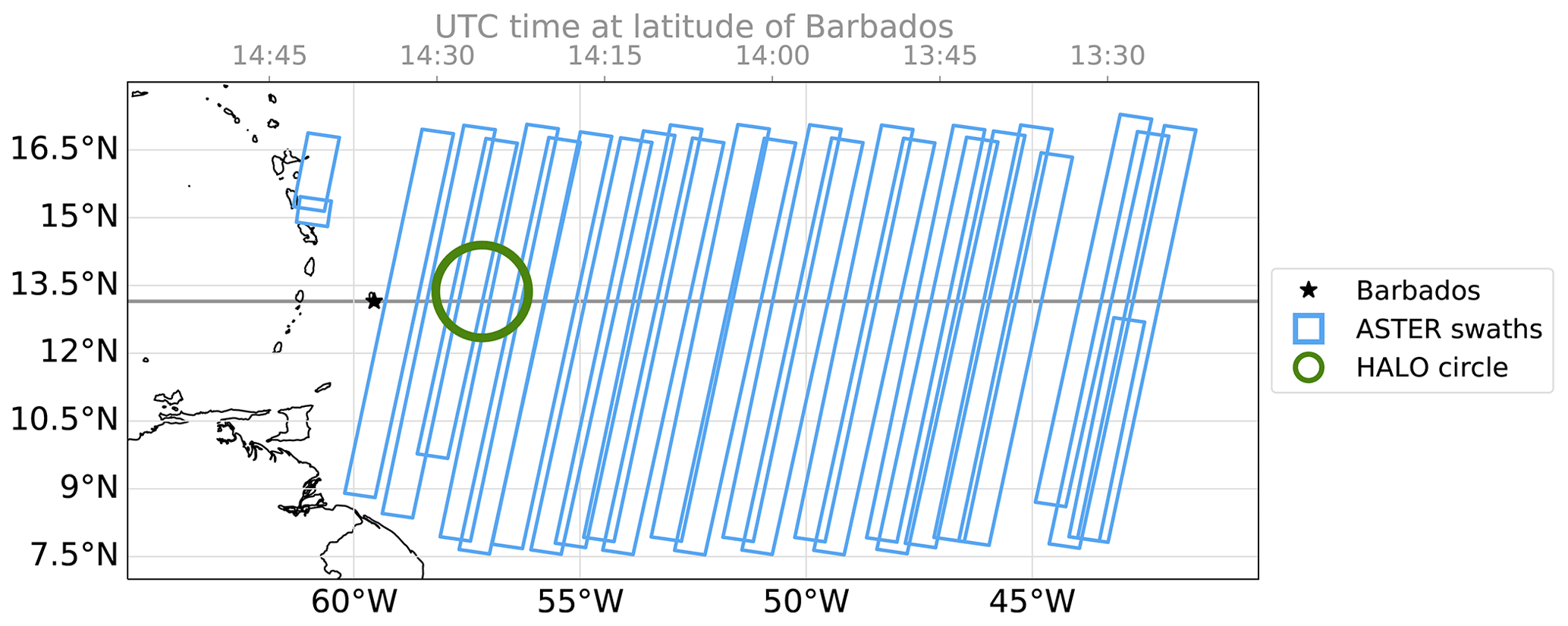
Figure 1 ASTER measurement locations during EUREC⁴A with 419 images (60 km×60 km) recorded on 17 d between 11 January and 19 February 2020. WALES lidar measurements are available from HALO's research flights predominantly on the circular path shown in green from 13 flight days between 22 January and 15 February 2020.

2.1 The ASTER dataset for EUREC⁴A

ASTER is mounted aboard Terra, a polar‐orbiting satellite in a descending Sun-synchronous orbit with an Equator crossing time of 10:30 local solar time. Terra crosses the latitude of Barbados and the HALO flight circle area roughly at 14:25 UTC, while the tracks further east at about 43^∘ W are observed by ASTER an hour earlier. Figure 1 shows the location of measurements taken in the area east of Barbados from 7 to 18^∘ N and from 41 to 62^∘ W between 11 January and 19 February 2020. The data from the observed swaths are segmented in the form of 60×60 km² images, each corresponding to 9 s of observation time.

ASTER's visible and near-infrared (VNIR) radiometer pointing nadir has three bands in the range of 0.53–0.86 µm. The radiometrically calibrated and geometrically coregistered Level 1B data provide top-of-atmosphere monodirectional radiances at 15 m pixel resolution at the sub-satellite point. We use the band 3 radiance centered at 0.807 µm in the present study to define the total cloud cover. One image of band 3 radiances consists of 4200 pixels along-track and 4980 pixels across-track with, depending on the viewing angle, about 15.4 % swath edge pixels that are neglected within the further analysis, leaving about 17 684 552 pixels per image.

In our analysis we work with reflectance instead of radiance with the aim to reduce the influence of varying solar zenith angles θ₀ within the overpasses and slightly varying extraterrestrial solar irradiance E₀. The reflectance R is calculated from the radiance L as

$$\begin{array}{}\text{(1)}& R={\displaystyle \frac{\mathit{\pi }L}{\cos \left({\mathit{\theta }}_{\mathrm{0}}\right)E_{\mathrm{0}}}}.\end{array}$$

We further draw comparisons to the ASTER cloud mask, which is based on several bands in the VNIR (Werner et al., 2016). The cloud mask works with thresholding tests and is representative for traditional passive remote sensing cloud-masking schemes such as the Moderate Resolution Imaging Spectroradiometer (MODIS) cloud detection scheme. In more detail, the algorithm uses three tests to distinguish between bright clouds and the dark ocean from thresholds applied to radiance values in the VNIR range. An additional test based on a band in the shortwave infrared (SWIR) is no longer applicable as the SWIR detector broke in 2007. Nevertheless, the three thresholding tests allow us to distinguish between confidently clear, probably clear, probably cloudy, and confidently cloudy pixels following the method described in Werner et al. (2016). Within the current study we combine the flags probably cloudy and confidently cloudy if we refer to cloudy regions according to the ASTER cloud mask. We omit a fifth test including ASTER's thermal band 14 (11.65 µm, 90 m pixel resolution) that is designed to detect cirrus-contaminated areas and Sun glint at the expense of a lower resolution. The observations during EUREC⁴A are luckily recorded at a minimum Sun reflection angle larger than 23^∘, making Sun glint highly unlikely.

Concerning cirrus cases, we decided to stay with the high resolution, but instead exclude images that have a high likelihood to be contaminated by cirrus clouds. A test based on the ratio of ASTER's thermal bands 13 and 14 is implemented following a publication by Hulley and Hook (2008). Next to cirrus, the test unfortunately also detects low thin clouds, the latter being the main actor of the current study, which we therefore want to keep in the dataset. Most importantly, we notice that our main results and statements change only marginally, indicating that cirrus does not have a strong impact on the current study. Nevertheless, we exclude images that have a chance of more than 10 % coverage by potential cirrus as defined by Hulley and Hook (2008), which leaves 380 images for our analysis.

2.2 WALES airborne lidar measurements

The WALES lidar instrument (Water Vapor Lidar Experiment in Space demonstrator; Wirth et al., 2009) is part of the remote sensing package that was on board the HALO research aircraft during EUREC⁴A (Stevens et al., 2019). The aircraft flew at about 9 km of altitude throughout of the campaign and thus below the typical altitude of cirrus clouds in the trades. We therefore do not expect any cirrus contamination in the WALES dataset. The high-spectral-resolution lidar measurements from the auxiliary channels of the instrument at 532 nm are well suited to investigate small and optically thin clouds due to the high instrument sensitivity to small particles ranging from aerosols to cloud droplets. The advantage of WALES compared to spaceborne active instruments such as the Cloud–Aerosol Lidar with Orthogonal Polarization (CALIOP) simply lies in the closer distance and thus higher sensitivity to low clouds as well as the much higher horizontal sampling due to the lower aircraft speed (0.2 versus 7 km s⁻¹). The resulting horizontal spatial resolution of the WALES cloud product is about 40 m during EUREC⁴A, which is slightly larger but commensurate with that of ASTER. CALIOP has been shown to struggle in detecting small clouds with cloud tops below 1 km (Leahy et al., 2012), while we find 29 % of clouds detected by WALES during EUREC⁴A to have cloud tops below 1 km.

Within the present study we use the cloud mask and cloud optical depth product described in Konow et al. (2021). In the dataset, a cloud is defined as having a backscatter ratio that exceeds 10. This threshold is lower compared to the studies by Gutleben et al. (2019) and Jacob et al. (2020) wherein the value was chosen to make the detection limit comparable to CALIOP. The lower value used in the present study nicely separates the highest possible signals originating from marine aerosol and any cloud-related signal that might include anomalously humidified aerosols and the smallest cloud droplets. WALES uses the high-spectral-resolution lidar technique (HSRL; Esselborn et al., 2008) to distinguish molecular from particle backscatter at 532 nm, which allows for the direct measurement of the (two-way) atmospheric transmission. The latter is proportional to the range (r) and atmospheric-density-corrected lidar signal R_M(r). To a first approximation the optical thickness is given by

$$\begin{array}{}\text{(2)}& \mathit{\tau }=\mathrm{-}{\displaystyle \frac{\mathrm{1}}{\mathrm{2}}}\cdot \ln \left({\displaystyle \frac{R_{\mathrm{M}}\left(r\right)}{R_{\mathrm{M}}\left(\mathrm{0}\right)}}\right).\end{array}$$

The complete algorithm adds several corrections and is described in detail in Esselborn et al. (2008).

2.3 Surface wind speed estimates

For the methodology described in Sect. 3 we need surface wind speed estimates at 10 m of height for a given ASTER pixel. The fifth-generation European Centre for Medium-Range Weather Forecasts reanalysis (ERA5) provides hourly wind speed estimates on a global grid at 10 m of height (2D surface product), which would fit our needs but showed a significant underestimation compared to collocated dropsonde measurements during EUREC⁴A (JOANNE dropsonde dataset: George et al., 2021). The underestimation is in agreement with a study by Belmonte Rivas and Stoffelen (2019), who find a low bias in ERA5 surface winds in the trades. Nevertheless, wind speed estimates from the ERA5 profile product (hourly, 0.25^∘ grid; Hersbach et al., 2020) agree remarkably well with dropsonde measurements.

Thus, we use ERA5 wind speeds at the lowest-altitude pressure level of 1000 hPa, which corresponds to about 135 m above sea level on average based on the dropsonde dataset. We derive a correction that translates from 1000 hPa to 10 m based on a comparison of ERA5 wind speed at 1000 hPa and the 10 m wind speed from dropsonde measurements (Pearson correlation coefficient 0.88). A least-squares fit provides us with the coefficients to estimate the 10 m wind speed by

$$\begin{array}{}\text{(3)}& \text{ws}=\mathrm{0.92}\cdot {\text{ws}}_{\mathrm{ERA}\mathrm{5},\mathrm{1000}\mathrm{hPa}}+\mathrm{0.40}.\end{array}$$

This wind speed is an average value representative for a 0.25^∘ grid cell. We therefore use measurements at the Barbados Cloud Observatory (BCO) to estimate the variance in wind speed within 0.25^∘ compared to the 15 m ASTER grid. The BCO is located at the easternmost point of the island of Barbados and has been shown to take measurements representative of an undisturbed marine trade wind boundary layer (Stevens et al., 2016). We use the standard surface wind speed measurements from a Vaisala WXT-520 to derive an estimate of the surface wind variance within 0.25^∘ (27.12 km at 13^∘ N), which translates to about an 80 min sampling period. We add a Gaussian perturbation according to the estimated wind variance of 1.63 m² s⁻² to the average wind speed within our further analysis. The campaign average wind speed corresponding to the ASTER image locations is 9.02 m s⁻¹.

3 Methodology

The ASTER cloud mask provides us with a good perception of the certainly clear and certainly cloudy areas, while we are less confident in between. We approach the intermediate range from the cloud-free by simulating the expected probability distributions of cloud-free reflectance for a given ASTER image. Knowing the theoretical cloud-free contribution to an all-sky ASTER image, we can then investigate the cloud-related contributions that are undetected by the cloud mask and which we attribute to optically thin clouds. 3D cloud radiative effects are a potential complicating factor in broken cloud conditions and we will discuss their influence in Sect. 4.3 together with results from the WALES lidar.

First, we introduce the methodology with a brief overview of the cloud-free retrieval setup and the necessary input information on surface wind speed and aerosol optical depth, before we show our approach for transferring the cloud-free information to the all-sky ASTER observations and defining areas of optically thin clouds.

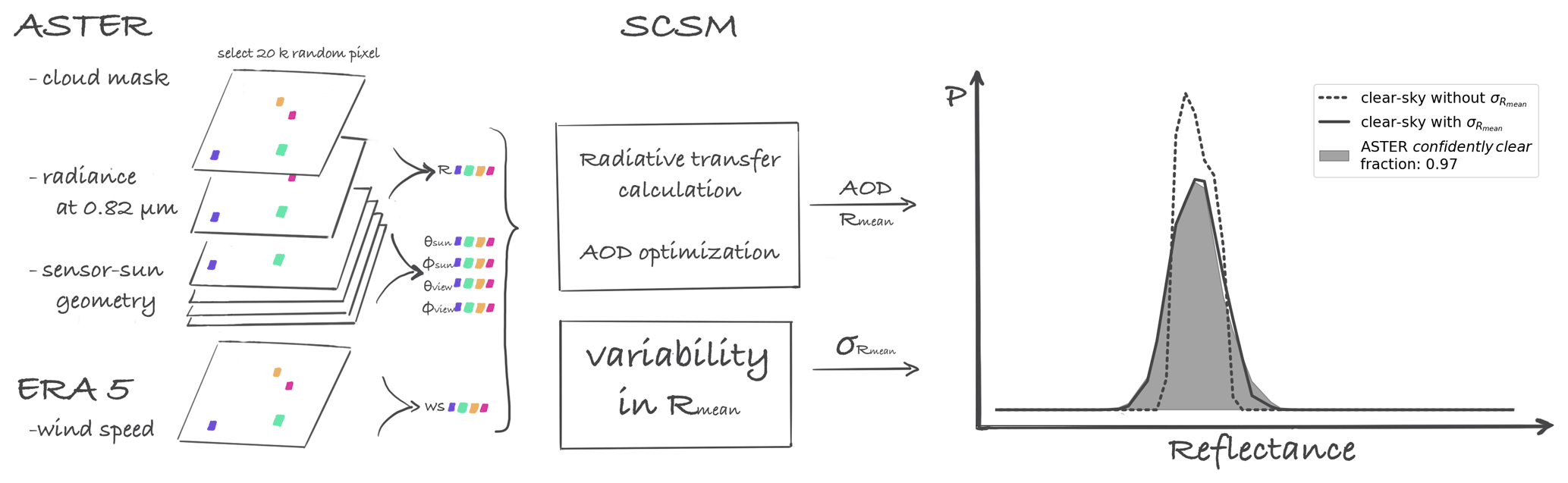
Figure 2 Sketch illustrating the cloud-free retrieval workflow. ASTER and ERA5 input data are used to run radiative transfer simulations with integrated AOD optimization. A Gaussian perturbation is added to the output average pixel reflectance R_mean to account for ocean surface variability and measurement noise. On the right are the processing steps that lead to the simulated cloud-free reflectance distribution for a single ASTER image observed on 24 January 2020 at 14:02:02 UTC.

3.1 A simplified clear-sky model (SCSM)

The cloud-free radiance over ocean in the visible range depends on a narrow set of parameters and can be estimated by simplified one-dimensional radiative transfer calculations. In Appendix A we describe the full set of equations and approximations made in calculating the cloud-free signal with our simplified clear-sky model (SCSM). We generally assume a single-layer atmosphere with constant air density and calculate the extinction of solar radiance from the top of the atmosphere to the ground and back to the sensor in space. How the light is reflected at the surface in the view direction of the sensor is characterized by the bidirectional reflection function, which depends on the surface wind speed and the generated ocean wave slope distribution. Here, we use the wind speed estimates described in Sect. 2.3 as input to the Cox and Munk parameterization to derive an average reflectance for a given surface condition (Cox and Munk, 1954).

We further need to know the aerosol optical depth (AOD) to estimate the extinction of direct and diffuse radiation on its path through the atmospheric column. Although the aerosol load does not vary much within a 60×60 km² ASTER image, the availability of aerosol information from measurements, even for an image-average AOD, is very limited. Therefore, we estimate an effective AOD in an optimization approach by including information from the ASTER dataset. We assume that the pixels labeled confidently clear in the ASTER cloud mask are a good first guess for cloud-free and shall serve as a reference for finding a suitable effective AOD such that the simulated cloud-free values are in close agreement with the selected ASTER pixel values.

In Fig. 2 we illustrate the cloud-free retrieval workflow. In detail, we randomly select 20 000 pixel (0.11 % of valid image pixels) from those defined confidently clear by the ASTER cloud mask (see Sect. 2.1) for a given ASTER image. Simulating 20 000 samples ensures a proper representation of the cloud-free distribution at a manageable computational cost. For those input pixel locations we run the cloud-free model with the corresponding sensor–Sun geometries, surface wind speed estimates, and a first guess on the AOD. We further optimize this image AOD value iteratively by minimizing the summed squared difference between simulated and observed reflectances. Here, we make use of SciPy's implementation of the limited-memory Broyden–Fletcher–Goldfarb–Shanno algorithm (LM-BFGS) with bounds (SciPy version 1.5.2). The resulting effective AOD value is representative for the reflectance distribution of a single ASTER image. From all evaluated ASTER images we find a campaign average effective AOD of 0.077 (±0.051).

From comparing simulated cloud-free reflectance distributions to selected observed ones for manually checked and seemingly cloud-free ASTER observations, we find two things. First, the distributions agree very well in terms of their expected value. Second, the simulated distributions are more narrow compared to the observed ones as the Cox and Munk parameterization returns average pixel reflectance R_mean. We therefore introduce a variability in brightness in a post-processing step. We calculate a kernel density estimate with normal kernels characterized by a standard deviation ${\mathit{\sigma }}_{R_{\mathrm{mean}}}$ that is placed on each of the simulated reflectance values (Rosenblatt, 1956; Parzen, 1962). We derive a suitable value for ${\mathit{\sigma }}_{R_{\mathrm{mean}}}$ from comparing simulated cloud-free reflectance distributions and corresponding ASTER images that have at minimum 97 % confidently clear pixels in the ASTER cloud mask. From 22 cases we calculate the average ${\mathit{\sigma }}_{R_{\mathrm{mean}}}=\mathrm{0.0026}$ from a least-squares optimization, again using the LM-BFGS algorithm. We use a constant value for ${\mathit{\sigma }}_{R_{\mathrm{mean}}}$ for the whole dataset due to the lack of several cloud-free observations for various sensor–Sun geometries. However, the ASTER dataset is confined to a narrow set of sensor–Sun geometries and outside possible Sun glint observations such that we assume that a constant value is sufficient for our application.

3.2 Identifying optically thin clouds in all-sky observations

The output from our SCSM provides us with a distribution of cloud-free reflectance $p\left(R\right|F_{\mathrm{CLEAR}},B)$, which is the probability distribution of reflectance values R given that they originate from cloud-free area with the flag F=F_CLEAR and additional background conditions B. The background conditions include the sensor–Sun geometry, wind speed, and AOD and are covered by the SCSM by handling each image individually. In the following we evaluate the probabilities on an image basis and therefore omit the implicit condition on B in the notation. Further, we use standard notation whereby | means “given that” for conditional probabilities and “,” means “and” and symbolizes combined (or joint) probabilities. For example, the SCSM output is a conditional probability as the SCSM framework does not include any information on the general cloud-free fraction within one image.

In the following, we split the observed reflectance distribution of an ASTER image into the categories or flag values $F\in \mathit{\{}{F}_{\mathrm{CLEAR}},F_{\mathrm{OTC}},F_{\mathrm{CLOUD}}\mathit{\}}$. The ascending order of the flag values indicates the associated expected increase in reflectance. The darkest observed pixels originate form cloud-free ocean observations. Small cloud fragments and humidified aerosols slightly enhance the reflectance, though they are often undetected by the cloud-masking scheme. We characterize them as optically thin clouds (OTCs). The flag CLOUD refers to the cloudy pixels detected by the ASTER cloud-masking scheme (see Sect. 2.1). We know the CLOUD part of a distribution p(R,F_CLOUD) from the observation and we can infer the CLEAR contribution from the SCSM output. The all-sky reflectance distribution p(R) is built up by the arithmetic sum of combined probability distributions of R and the flag values F:

$$\begin{array}{}\text{(4)}& \begin{array}{rl}p\left(R\right)& =\sum _{F_{\mathrm{n}}}p(R,F_{\mathrm{n}})\\ & =p(R,F_{\mathrm{CLEAR}})+p(R,F_{\mathrm{OTC}})+p(R,F_{\mathrm{CLOUD}}).\end{array}\end{array}$$

Each combined probability can be represented by the product of the corresponding conditional probability and the probability of the flag value, i.e., for cloud-free

$$\begin{array}{}\text{(5)}& p(R,F_{\mathrm{CLEAR}})=p\left(R\right|F_{\mathrm{CLEAR}})\cdot p(F_{\mathrm{CLEAR}}).\end{array}$$

The probability of cloud-free p(F_CLEAR) is the true cloud-free fraction in an observed image and is challenging to estimate. Note that the true cloud-free fraction is independent of the ASTER cloud mask. If we knew the cloud-free fraction p(F_CLEAR), Eqs. (5) and (4) together would fully describe the observed reflectance distribution p(R). In the following we describe our approach for estimating the unknown cloud-free fraction.

The first constraint is given by the fact that any probability must be within the range [0,1], and thus we can formulate for our case

$$\begin{array}{}\text{(6)}& p\left(F_{\mathrm{CLEAR}}\right|R^{\prime \prime })+p(F_{\mathrm{CLOUD}}\left|R^{\prime \prime }\right)\le \mathrm{1}\forall R^{\prime \prime }\in R.\end{array}$$

We can approach the estimation of the cloud-free fraction p(F_CLEAR) from a conservative side by deriving the maximum possible p(F_CLEAR) such that Eq. (6) still holds. Thinking visually, we scale the simulated cloud-free distribution up until it touches the all-sky distribution p(R). At the reflectance $R=R^{\prime }$ (of unknown value) where the probability density functions (PDFs) touch, we are certain that the non-cloudy classified reflectances are actually due to cloud-free:

$$\begin{array}{}\text{(7)}& \exists R^{\prime }\text{ such that }p\left(F_{\mathrm{CLEAR}}\right|R^{\prime })=\mathrm{1}-p(F_{\mathrm{CLOUD}}\left|R^{\prime }\right).\end{array}$$

We can solve Eqs. (7) and (6) for p(F_CLEAR) (for details see Appendix B). While being mathematically concise, the described method faces a problem. It relies on the exact count of measurements in only a single reflectance bin R^′ and is thus especially susceptible to measurement and model uncertainties. We tackle this problem by extending and relaxing the condition stated in Eq. (7). We modify this first condition from a single value to an extended range of reflectance values. As Eq. (7) would be overdetermined for more than one reflectance value in the presence of measurement and model uncertainties, we demand that the equation approximates the value $\mathrm{1}-p\left(F_{\mathrm{CLOUD}}\right|R^{\prime })$ for reflectivity values measured and known to be caused by cloud-free skies.

In particular, we do this by a weighted linear regression, minimizing the term

$$\begin{array}{}\text{(8)}& \int {\left|\left[p\left(F_{\mathrm{CLEAR}}\right|R)-\left(\mathrm{1}-p\left(F_{\mathrm{CLOUD}}\right|R)\right)\right]\cdot w\right|}^{\mathrm{2}}\mathrm{d}R\end{array}$$

with p(F_CLEAR) as the only free variable. The regression weight $w=p\left(R\right)p\left(R\right|F_{\mathrm{CLEAR}})$ is chosen to only consider measured reflectance p(R) that overlaps with the range of simulated cloud-free reflectance p(R|F_CLEAR). The product of both guarantees close agreement around the peaks of measured and simulated PDF.

The resulting estimate of p(F_CLEAR) is more robust in the presence of small measurement or model errors, but a direct consequence of this approximate matching is that Eq. (6) does not necessarily hold for all R^′′ anymore. As illustrated in Fig. 3 using dotted and dashed lines, we correct this by clipping the resulting probabilities to the allowed range. As this clipping effectively modifies the simulated reflectance distribution and is thus potentially dangerous, we need to ensure that this method indeed only compensates for small measurement uncertainties (i.e., of the order of a single digital sensor count). We can do this by comparing the expected value of the clear-sky reflectance p(R|F_CLEAR) before and after clipping. On average, this difference is 0.15 % and even in the worst (maximum) case, the clipping causes a shift of 0.0018 in reflectance units, which is well below one digital sensor count of about 0.004 reflectance units. Based on this analysis, we use the more stable regression and clipping method instead of a direct application of Eq. (7).

Further, the SCSM does not include cloud shadows on the ocean surface, which introduce a signal at very low reflectances in the observed distribution. Conceptually we add the low reflectance values originating from such shadowed areas to the cloud-free reflectance distribution p(R,F_CLEAR).

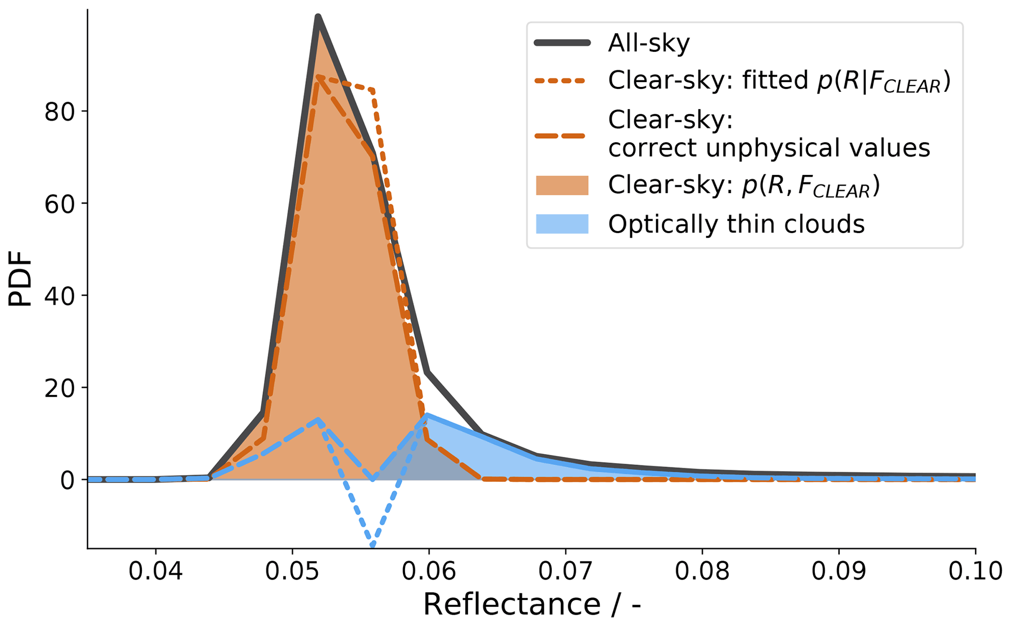
Figure 3 Visualization of the approach for estimating the cloud-free fraction p(F_CLEAR) by optimization. The orange dotted and dashed lines show the processing steps leading to the filled orange cloud-free PDF. The blue lines are the respective residuals related to optically thin clouds and resulting from the all-sky (grey) minus the CLEAR (orange) and minus the CLOUD PDF (dark blue; not visible).

In Fig. 4 we show combined probability distributions per flag for an ASTER observation on 31 January east of Barbados. The inset shows the reflectance image that we translate into the distribution using the method described above.

Figure 4 Reflectance distribution corresponding to the ASTER observation shown in the inset recorded on 31 January 2020 at 14:08:05 UTC southeast of the HALO circle area at 11.37^∘ N, 53.86^∘ W. The cloud-free contribution is retrieved with the method (1) described in Sect. 3.2 and displayed by the orange curve, while pixel reflectances identified as cloudy from the ASTER cloud-masking algorithm are shown in dark blue. We attribute the light blue contribution to the distribution to optically thin clouds.

3.3 Robustness of optically thin cloud estimation

Our target variables are the fraction and expected reflectance of optically thin clouds. The retrieval of cloud-free and subsequent optically thin clouds in ASTER images depends on visible cloud-free areas, which limits the evaluation of the full ASTER EUREC⁴A dataset to images with less than 85 % detected cloud cover in the cloud-masking algorithm (380 images).

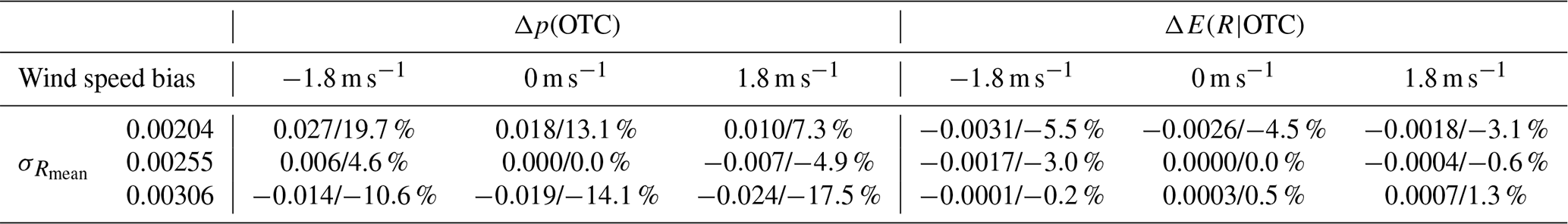
Within the retrieval we have two main free parameters which can introduce uncertainty in our target values: the surface wind speed estimate and the assumed variability ${\mathit{\sigma }}_{R_{\mathrm{mean}}}$ of simulated average pixel reflectances R_mean. We first have a look at the added variability. From a comparison of 22 manually checked cloud-free reflectance distributions (>97 % confidently clear pixels) to the simulated distributions we derived an average variance of 0.0026 (±0.0007). We apply the methodology described in this section for the average value, as well as for a 20 % lower (0.0020) and 20 % higher value (0.0031). Similarly, we add an artificial bias of ±20 % to the surface wind speed estimates and investigate the change in our target values. The average wind speed in our dataset is 9.02 m s⁻¹ (±2.38 m s⁻¹). The resulting deviations in our target values, the fraction p(OTC) and expected reflectance E(R|OTC) of optically thin clouds, that result from a bias in ${\mathit{\sigma }}_{R_{\mathrm{mean}}}$ and/or the surface wind speed are stated in Table 1.

The fraction of optically thin clouds p(OTC) changes only slightly with a change in wind speed, showing an overestimation for a negative wind speed bias, meaning that a small part of the cloud-free distribution is wrongly attributed to optically thin clouds. For a positive wind speed bias the opposite is the case. The low uncertainties (4.6 % and −4.9 %) are a result of the retrieval setup including the optimization of AOD, which can partly compensate for a bias in wind speed. Changing the variability of simulated average pixel reflectances ${\mathit{\sigma }}_{R_{\mathrm{mean}}}$ can narrow (negative bias in ${\mathit{\sigma }}_{R_{\mathrm{mean}}}$) and broaden (positive bias in ${\mathit{\sigma }}_{R_{\mathrm{mean}}}$) the cloud-free distribution and thus lead to strong overestimation or underestimation of p(OTC) as high as 13.1 % and −14.1 % (relative deviations). Combining the highest retrieval uncertainties from the two free parameters, the wind speed and the variability ${\mathit{\sigma }}_{R_{\mathrm{mean}}}$, we can get a deviation in the estimated fraction of optically thin clouds of up to ±0.027 (relative: ±19.7 %).

The expected reflectance of optically thin clouds E(R|OTC) shows a smaller sensitivity to changes in the wind conditions and ${\mathit{\sigma }}_{R_{\mathrm{mean}}}$ compared to the fraction of optically thin clouds discussed above. An underestimation in wind speed leads to a marginal underestimation in the expected reflectance as lower cloud-free reflectance is wrongly attributed to optically thin clouds. In the case of an overestimation in wind speed, the cloud-free reflectance distribution extends to higher reflectance values, which are missing in the estimated E(R|OTC), and thus leads to a high bias in E(R|OTC). A more narrow (negative bias in ${\mathit{\sigma }}_{R_{\mathrm{mean}}}$) or broader (positive bias in ${\mathit{\sigma }}_{R_{\mathrm{mean}}}$) cloud-free distribution can decrease or increase the expected reflectance of optically thin clouds up to −4.5 %. However, the combined deviation due to possible biases in wind speed and ${\mathit{\sigma }}_{R_{\mathrm{mean}}}$ is still within the range of ± 0.0031 (± 5.5 %), which is smaller than the reflectance bin size of the original Level 1B ASTER data (least significant bit).

Table 1 Deviations of the fraction Δp(OTC) and expected reflectance ΔE(R|OTC) of optically thin clouds for the two main free parameters from the clear-sky retrieval, the surface wind speed, and the variability ${\mathit{\sigma }}_{R_{\mathrm{mean}}}$. The two numbers in each cell state the absolute and relative difference to the reference case with no wind speed bias and ${\mathit{\sigma }}_{R_{\mathrm{mean}}}=\mathrm{0.0026}$, respectively.

4 Results

We investigate 380 ASTER images for the signal from optically thin clouds (OTCs) that are undetected by the ASTER cloud mask but can be identified with the method described in Sect. 3. We first visualize pixels in an image that we attribute to the total cloud cover including OTC pixels and those detected in the ASTER cloud mask. We then define a close match of OTC reflectances in ASTER images and the signal of OTC detectable in WALES lidar data. WALES measurements provide an independent view of the results of the cloud cover by OTC from a different instrument technology and complement our analysis based on ASTER images. Finally, we show the significant contribution of optically thin clouds to the total cloud cover.

4.1 Visualizing optically thin clouds in an ASTER image

To visualize the OTC area in an image we can define a threshold in reflectance similar to common cloud-masking algorithms. We construct a total cloud cover mask that includes pixels with a probability of that pixel reflectance to be cloudy $p\left(F_{\mathrm{TOTAL}\mathrm{\_}\mathrm{CLOUD}}\right|R=R_{\mathrm{pixel}})\ge \mathrm{0.9}$ with $F_{\mathrm{TOTAL}\mathrm{\_}\mathrm{CLOUD}}=F_{\mathrm{OTC}}\vee F_{\mathrm{CLOUD}}$. In the particular ASTER image shown partially in Fig. 5 all reflectance values greater than 0.049 satisfy that condition. The cloud mask derived with the cloud-masking algorithm by including several ASTER bands is shown in blue in panel (a), while the total cloud cover mask is shown by the contours in red in panel (b). The background reflectance image in panel (b) is adjusted in its reflectance range with the aim of enhancing the range reflectances related to OTC.

The figure visualizes how OTC is often classified in pixels surrounding detected clouds. Detraining clouds and anomalously humidified aerosols likely cause enhanced reflectances close to thicker clouds. Possible scattering of light at the sides of thicker clouds might additionally enhance the brightness of their surrounding areas. Such surrounding halos of optically thin clouds lead to (threshold-dependent) smoother cloud edges, an interesting result in the context of cloud boundaries and related fractal dimensions. Also, cloud structures tend to be more connected in the total cloud cover mask, leading to larger cloud objects with smooth reflectance transitions to the cloud-free ocean background. While there are numerous studies on cloud shapes, we rather focus on a statistical estimate of area coverage and the contribution of OTC to the total cloud cover in the remainder of this work.

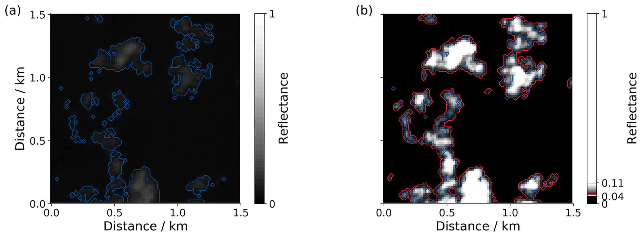
Figure 5 Visualization of the area corresponding to optically thin clouds. Shown are reflectances at 0.807 µm for a 1.5×1.5 km² selection of an ASTER image recorded on 5 February 2020 at 14:25:15 UTC. (a) The full physical range of reflectance values ranging from 0 to 1 with overlaid blue contours outlining the ASTER cloud mask. (b) Similar to (a) but with the color scale limited to the 10th and 90th percentile of reflectances attributed to total cloud cover including optically thin clouds. The red contours correspond to $p\left(F_{\mathrm{TOTAL}\mathrm{\_}\mathrm{CLOUD}}\right|R=R_{\mathrm{pixel}})\ge \mathrm{0.9}$.

4.2 The OTC equivalence in lidar data

In Fig. 5 optically thin clouds are barely visible in the reflectance field in panel (a), suggesting that those clouds have a very low cloud optical thickness. Due to nonlinearities in the physical and radiative properties of small cumulus clouds and the large influence of 3D radiative effects, plane-parallel retrievals of microphysical properties do not work reliably and we cannot derive cloud optical thickness from ASTER measurements directly (Davies, 1978; Loeb et al., 1997; Várnai and Marshak, 2003; Marshak et al., 2006; Stevens et al., 2019; Kölling, 2020). However, we use the theoretical relationships that plane-parallel retrievals are based on to estimate an effective cloud optical thickness that could be detected by ASTER against the ocean surface background following the two-stream approximation by Lacis and Hansen (1974):

$$\begin{array}{}\text{(9)}& A={\displaystyle \frac{\sqrt{\mathrm{3}}(\mathrm{1}-g)\mathit{\tau }}{\mathrm{2}+\sqrt{\mathrm{3}}(\mathrm{1}-g)\mathit{\tau }}}\approx {\displaystyle \frac{\mathit{\tau }}{\mathit{\tau }+\mathrm{7.7}}},\end{array}$$

with the cloud albedo A, cloud optical thickness τ, and the asymmetry parameter g=0.85. In Fig. 6 we show the relationship stated in Eq. (9) of a plane-parallel cloud (black line) and add uncertainties from cloud 3D effects and the background ocean signal.

The average ocean reflectance during EUREC⁴A was 0.04 including single cases as high as 0.08. Due to additional variability in the ocean wave reflection we expect clouds with an albedo below 0.1 and corresponding cloud optical thickness below 1 to dissolve in the ocean signal. For clouds with cloud optical thickness larger than 1, 3D effects such as brightening and shadowing as well as photon loss through the cloud sides become relevant and can easily cause a factor of 2 error in the reflectance that spans a distribution around the plane-parallel estimate and that we indicate by the grey shaded area in Fig. 6 (Marshak et al., 2006; Stevens et al., 2019). Overall, we assume that due to natural variability in the background ocean signal and the cloud signal, clouds with optical thickness below 1 likely do not stand out from the ocean and the ASTER cloud mask is presumably insensitive to such optically thin clouds.

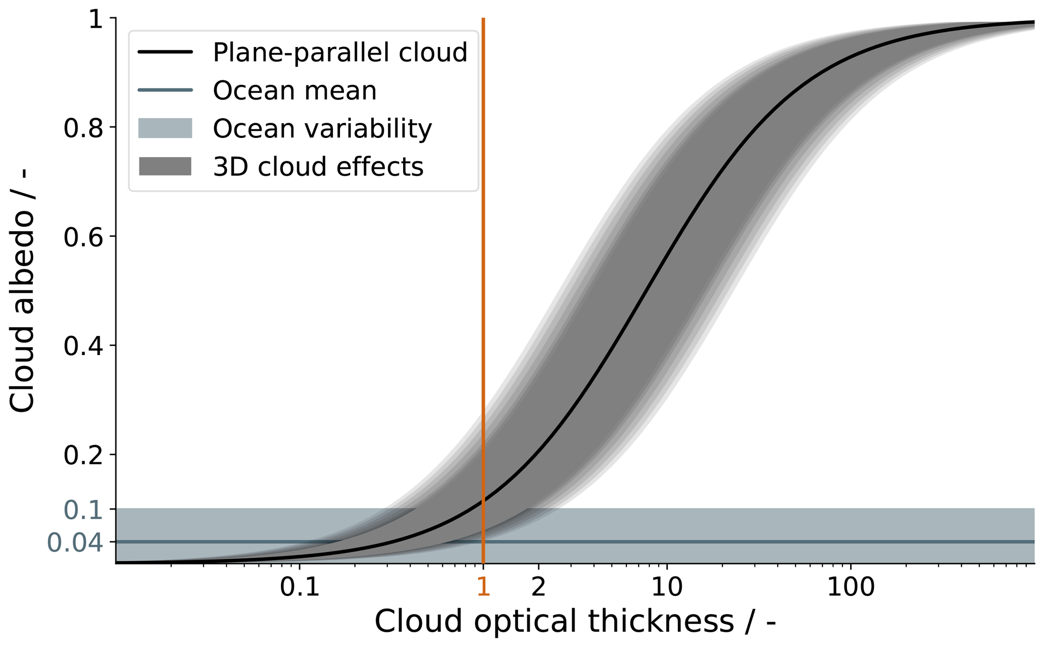
Figure 6 Plane-parallel relationship between cloud albedo and cloud optical thickness following Lacis and Hansen (1974). The ocean reflectance is estimated from the ASTER observations during EUREC⁴A, while the uncertainty due to 3D radiative effects is a rough estimate from the literature (Marshak et al., 2006; Stevens et al., 2019).

Clouds with an optical thickness below 1 are thin enough for a lidar beam to penetrate through the cloud and provide a reliable estimate of the cloud optical thickness. We can therefore make use of WALES lidar measurements for supporting information on the abundance of optically thin clouds.

Figure 7 shows the distribution of cloud optical thickness measurements from WALES for days with local research flights. The peak at low cloud optical thickness values corresponds to optically thin clouds that the lidar beam manages to penetrate. A cloud with optical thickness of about 2.5 reduces the lidar signal below the cloud to more than $\mathrm{1}/\mathrm{100}$, and the method to derive the optical thickness still works. At night the range of retrieved optical thickness increases to about 3.5 due to a better signal-to-noise ratio above clouds without scattered sunlight. In thicker clouds the signal vanishes in the system noise. We aggregate all measurements from optically opaque and thick clouds in one bin as we have no information on the actual cloud optical thickness.

In WALES measurements we associate optically thin clouds with an optical thickness below 1. The campaign average cloud optical thickness of OTC is 0.37, and the median is 0.31. Optically thin clouds have on average a cloud-top height at 1.3 km of altitude (median 1.0 km). We further use the WALES measurements to derive a fractional cloud cover in time for optically thin clouds and compare the results to the optically thin cloud cover from ASTER in the following section.

Figure 7 Cloud optical thickness distribution from WALES lidar measurements for all days with local research flights during EUREC⁴A resulting in 92 h of data. Panel (a) shows the frequency distribution of all days, while panel (b) additionally shows the cumulative distributions for individual days. The days are sorted by their increasing average cloud optical thickness that we associate with optically thin clouds (yellow to dark green). The split x axis visualizes the limited information on thick clouds that are optically opaque to the lidar.

Table 2 Cloud cover estimates during EUREC⁴A from 380 ASTER satellite observations (60×60 km²) at 15 m resolution on 17 d and from WALES lidar measurements recoded within 13 research flights (days) at about 40 m resolution in January and February 2020.

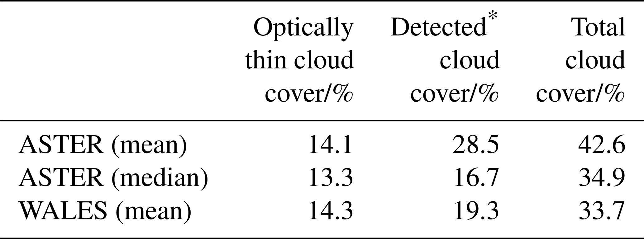
^* “Detected” refers to the ASTER cloud mask and, in the case of WALES data, to clouds with cloud optical thickness ≥1.

4.3 The contribution of OTC to the total cloud cover

From analyzing 380 ASTER images during EUREC⁴A we find an average total cloud cover of 42.6 %, combined of 28.5 % from detected clouds and 14.1 % from optically thin clouds (see Table 2). Based on the cloud-free retrieval uncertainties derived in Sect. 3.3 we estimate the uncertainty in ASTER optically thin cloud cover to be within the range of ±2.7 %. In Table 2 we state the respective numbers derived from WALES measurements. We explicitly note that a direct comparison is not reasonable as the two instruments and approaches show optically thin cloud areas from two different perspectives. However, what we can say is that WALES lidar measurements indicate high fractional coverage by optically thin clouds, similar to what we find from ASTER images.

In Sect. 4.1 we mentioned the possible influence of scattering at cloud edges, which can illuminate areas surrounding thicker clouds. Such 3D effects would influence our results based on ASTER data and lead to an overestimation of OTC-related cloud cover. As WALES is less affected by the 3D scattering at cloud edges but shows a higher fraction of optically thin clouds (42.4 %) relative to ASTER (33.1 %), the ASTER analysis does not seem to be unduly influenced by 3D radiative effects.

Our results based on ASTER and WALES measurements are lower compared to an analysis of optically thin marine clouds from CALIOP measurements by Leahy et al. (2012). The authors find a fraction of optically thin clouds in the trades to be as high as 84 %. From WALES measurements we derived an OTC fraction of 42.4 % for cloudy profiles with cloud optical thickness <1. If we include clouds with cloud optical thickness up to about 3, as is done in the study by Leahy et al. (2012), the OTC fraction in WALES data increases to 74 %. Estimates based on CALIOP data are likely to overestimate the OTC fraction due to the lower sensor resolution of 90 m footprints every 335 m. Leahy et al. (2012) derive a possible overestimation of OTC fraction of up to 25 % in the trades due to partially cloudy CALIOP footprints, which supports our findings in the current study of a lower but still significant contribution of optically thin clouds to the total cloud cover.

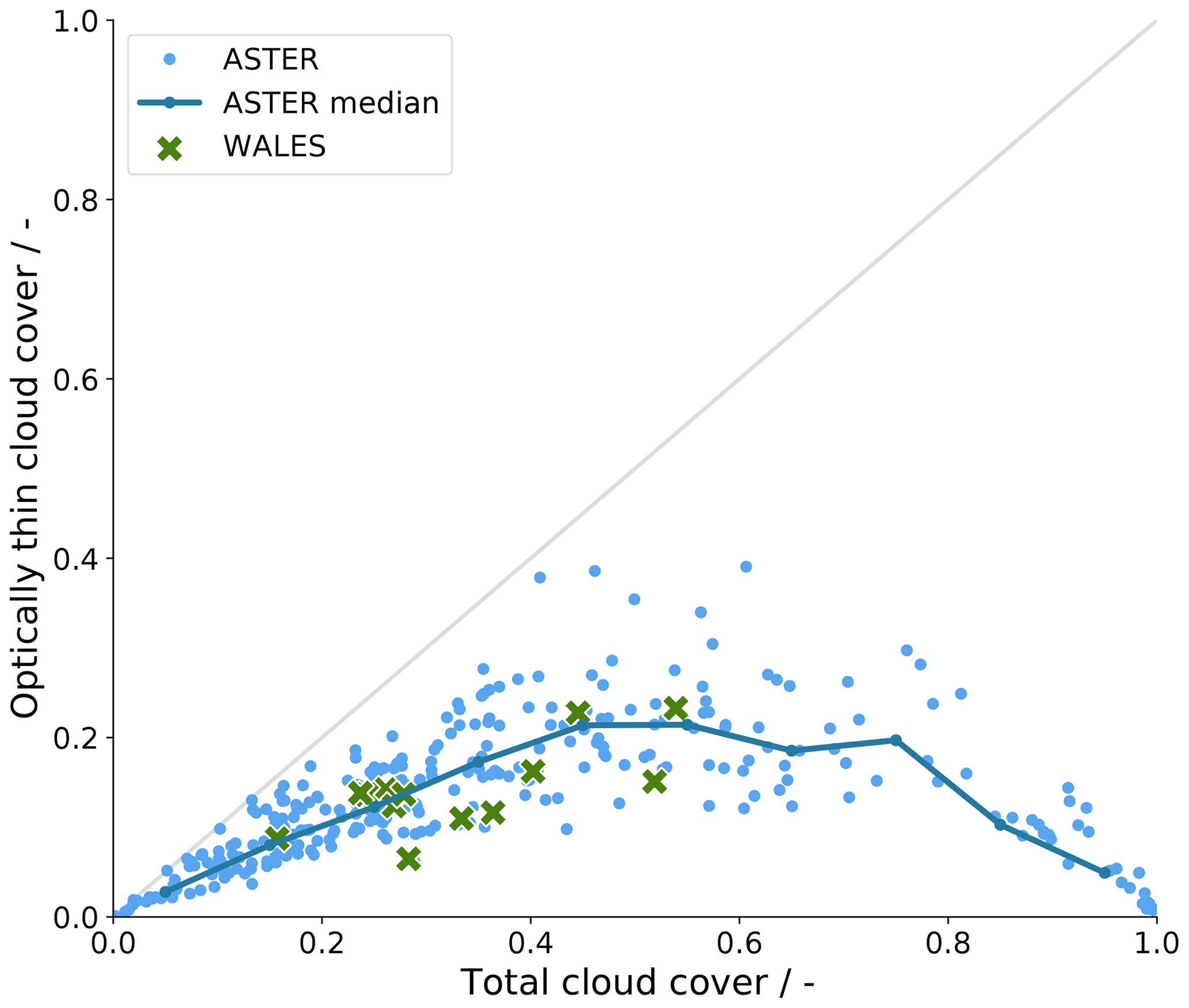
Figure 8 Change in optically thin cloud cover with total cloud cover. The blue markers correspond to values derived from 380 ASTER images (60×60 m²), with the dark blue line following along the median values. The green markers correspond to daily averaged cloud cover estimates from WALES lidar measurements. The grey diagonal line shows the maximum possible contribution of optically thin clouds to the total cloud cover.

We further notice that the area covered by optically thin clouds increases with detected cloud cover for low total cloud cover as shown in Fig. 8 and similarly stated in Leahy et al. (2012). The positive correlation up to 0.4 total cloud cover might be due to a combination of two features. First, optically thin cloud areas are often found surrounding detected clouds (see also Fig. 5). This idea is supported in a study by Koren et al. (2007), who find enhanced reflectances in solar irradiance measurements before and after an identified cloud originating from humidified aerosols and/or unresolved cloud fragments.

The second ingredient to the proposed positive correlation is the cloud field structure. Trade wind cumulus cloud fields at low cloud cover typically correspond to sugar or gravel type structures as described by Stevens et al. (2020), consisting of many small clouds with enough space in between that can be partly filled with undetected optically thin clouds. More clouds and a more cloud boundary therefore lead to more optically thin cloud area up to a point at which this relationship saturates at about 0.4 total cloud cover. The saturation might be due to larger clouds or cloud structures being surrounded by pronounced cloud-free regions. A recent study by Schulz et al. (2021) identifies the so-called flower and fish cloud patterns of having characteristic cloud-free areas between clouds. By constraint, the positive correlation turns negative above 0.7 total cloud cover as the cloud-free, OTC, and detected cloud cover always add up to 1, and high-cloud-mask cloud cover situations leave little space for optically thin clouds.

We conclude that optically thin clouds cover large parts of the trades, leading to a higher total cloud cover than assumed so far from passive satellite observations.

4.4 The cloud reflectance–cloud cover relationship in ASTER observations

Current climate models typically have a narrow range of cloud optical thickness that might affect model perturbation experiments due to the nonlinearity of cloud optical thickness and its albedo. Especially in low-cloud regions such as the trades, climate models underestimate the cloud cover while overestimating its average reflectance, a problem often called the “too few, too bright” low-cloud problem (Nam et al., 2012; Klein et al., 2013). While observations show a positive correlation of cloud cover and cloud reflectance, models show a reverse sign (Konsta et al., 2016).

We investigate the cloud cover–cloud reflectance relationship in Figs. 9 and 10. Figure 9a shows in blue curves the change in all-sky reflectance distribution with increasing cloud cover as defined by the ASTER cloud mask, while the red lines similarly show the change with increasing total cloud cover. We show two representative cloud cover ranges: a low range from 0.1 to 0.3 and a high range from 0.5 to 0.7. With increasing cloud cover, the reflectance distributions shift to higher values, meaning that the overall image is brighter (dashed versus solid lines). As expected, the reflectance distributions as defined by our method (red lines, including optically thin clouds) peak at lower reflectance values compared to their ASTER cloud-mask counterparts, meaning that the total cloud cover area is less bright on average when optically thin clouds are included.

Panel (b) shows an interesting new facet to the difference in total and cloud-mask cloudy areas. The distributions show how the total cloud reflectance relative to the total cloud area in the image depends on cloud cover. The comparison of low- and high-cloud-cover cases reveals that clouds are brighter with increasing cloud cover (dashed versus solid lines), which is in agreement with our perception of larger, deeper, and brighter clouds being present in high-cloud-cover situations. The change in cloud brightness with cloud cover is less pronounced if the total cloud cover is considered (red lines, including optically thin clouds) compared to the cloud-mask-only case (blue lines).

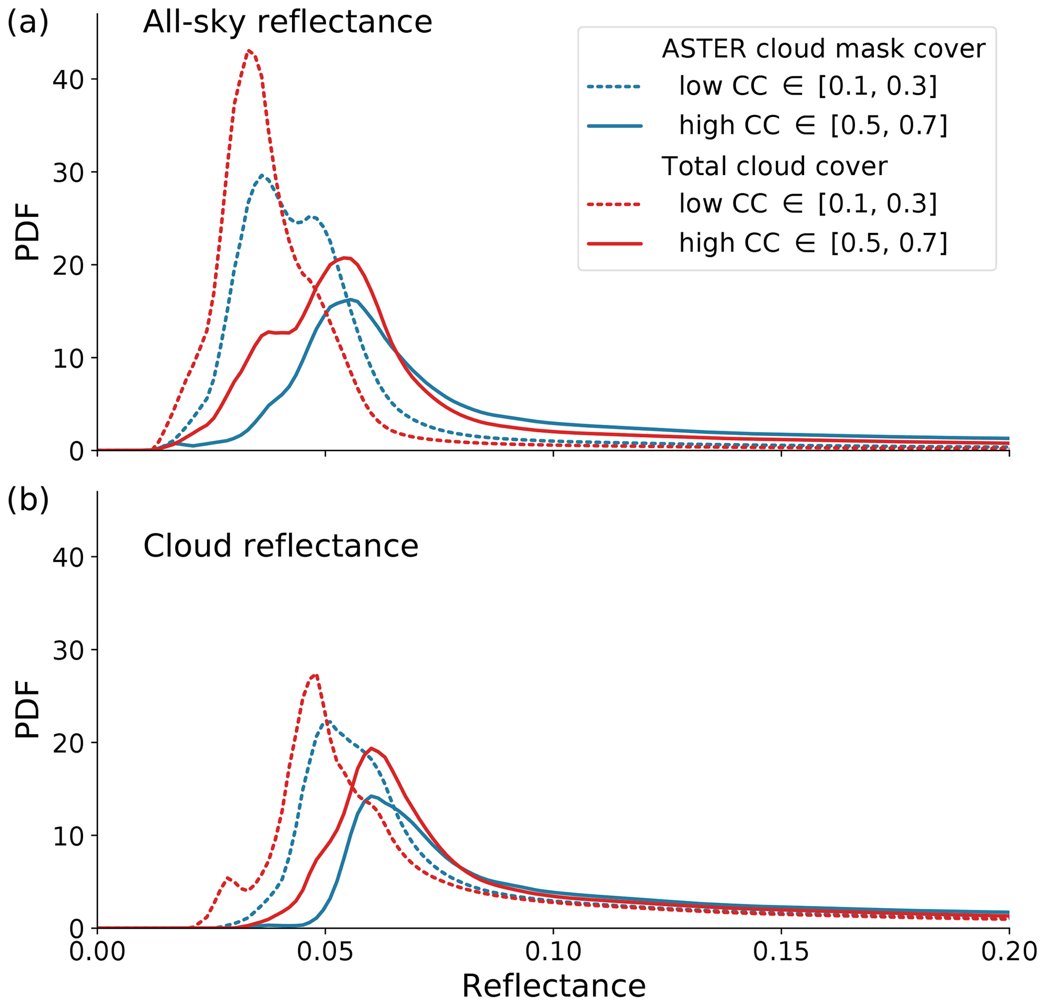
Figure 9 Combined probability density functions (PDFs) of (a) all-sky reflectance from ASTER p(R|CC), binned according to the total (red) and cloud-mask (blue) cloud cover (CC). We define two representative cloud cover ranges: low CC (0.1 to 0.3) and high CC (0.5 to 0.7). Panel (b) shows the conditional probability of total cloud reflectance p(R|F_TOTAL, CC), given that they are within the range of low or high CC. Compared to (a), the distributions in panel (b) do not include the cloud-free contributions at low reflectance.

We further investigate the expected cloud reflectance in relation to derived cloud cover values for all 380 ASTER images in Fig. 10. Both cloud-mask and total cloud cover exhibit positive correlations with respective cloud reflectance values, in agreement with findings in Konsta et al. (2016). We derive a campaign average cloud reflectance from total cloud cover of 0.15, with contributions from the ASTER cloud-mask clouds (average: 0.21) and optically thin clouds (average: 0.06), which agrees quite well with an average trade wind cumulus cloud reflectance of 0.15 derived from a combination of POLDER (Polarization and Directionality of the Earth's Reflectances) and CALIOP measurements in the study by Konsta et al. (2016). Based on the cloud-free retrieval uncertainty stated in Sect. 3.3, the uncertainty in expected reflectance of optically thin clouds is as low as 0.0031 and does not influence our results and conclusions drawn here.

The positive correlation in Fig. 10 for total cloud cover agrees well with the corresponding Fig. 6a in Konsta et al. (2016). As mentioned before, climate models show a reverse sign of this correlation together with a general underestimation of cloud cover and simultaneous overestimation of cloud reflectance. Next to the model intrinsic mechanisms leading to clouds that are too few but too bright, biases might be partially due to tuning the model based on traditional cloud masks that overestimate the cloud reflectance, especially in the frequent low-cloud-cover situations.

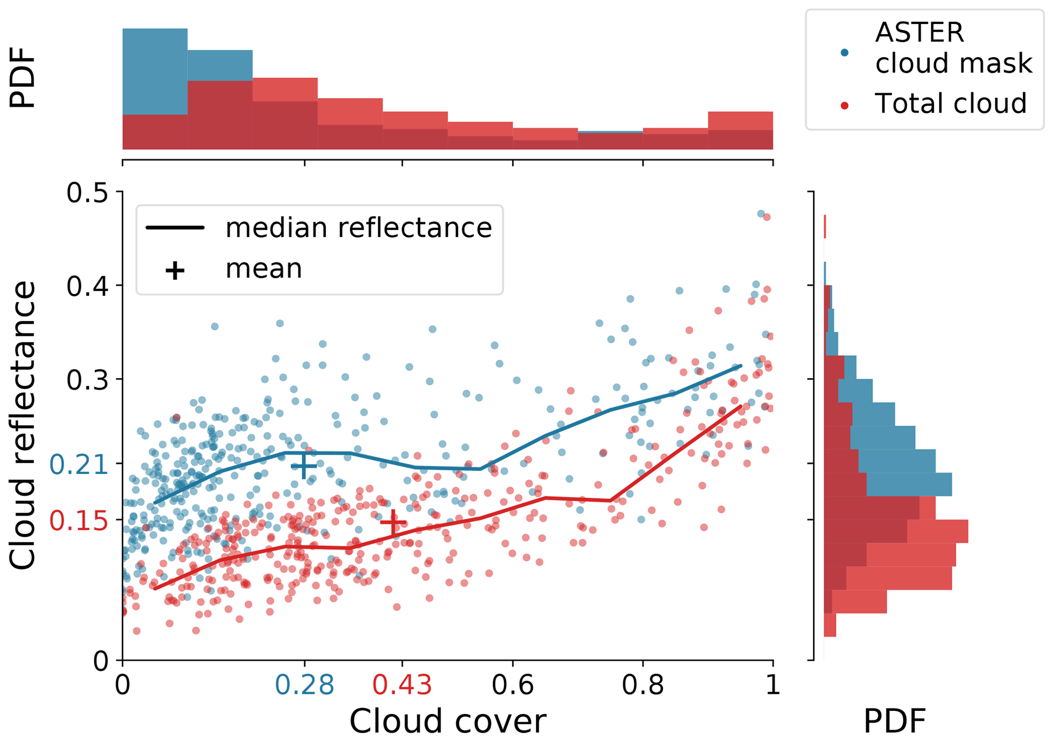
Figure 10 Expected cloud reflectance corresponding to the ASTER cloud mask (blue) and the derived total cloud cover (red) from 380 ASTER images. The median cloud reflectances are given by the lines, and the dataset averages are visualized by the + marker and the respectively colored tick labels. The frequency distributions of cloud cover and cloud reflectance are shown on the top and right, respectively.

5 Discussion

Most passive satellite imagers operate at resolutions of the order of hectometer to kilometer range and derive cloud products at 1 km scale or coarser. Undetected optically thin clouds, as well as small clouds detected at the ASTER 15 m scale, are unresolved and lead to partially cloudy pixel measurements. Several studies in the past have investigated the resolution effect in trade cumulus cloud cover estimated from passive satellite imagers. Zhao and Di Girolamo (2006) find a threefold to fivefold overestimation of cloud cover in MODIS and Multi-angle Imaging SpectroRadiometer (MISR) images, respectively, compared to ASTER observations during the RICO (Rain in shallow Cumulus over the Ocean) campaign. For the same dataset, a study by Dey et al. (2008) suggests a fourfold overestimation of cloud cover if the ASTER cloud mask is degraded from 15 m to 1 km while cloud detection thresholds are kept constant. However, degrading the resolution can also lead to an underestimation of cloud cover estimates in cloud-masking schemes if the resulting pixel radiances fall below fixed radiance thresholds. In an early study by Wielicki and Parker (1992) the authors estimate that roughly one-third of the cloud cover detected in 30 m Landsat images showing cumulus clouds would not be detected by certain cloud-masking schemes, which is in line with our study results.

An underestimation of cloud cover due to undetected optically thin clouds and an overestimation due to a reduced spatial resolution have compensating tendencies. However, one effect that does not cancel out in typical passive satellite cloud products is the influence of optically thin clouds in partially cloudy pixels that are classified to be clear. Pure cloud-free observations are crucial for aerosol retrieval and cloud radiative effect (CRE) estimates. With decreasing sensor resolution the probability for cloud-free observations decreases as well. We therefore investigate implications that undetected optically thin clouds can have on CRE estimates, as well as our inferences of cloud–aerosol interactions in the trades, despite their low cloud albedo.

5.1 Implication for CRE estimates

In temperature perturbation studies, cloud feedback defines how clouds adjust to a perturbation in surface temperature and whether this change amplifies or dampens the initial temperature perturbation. As such, it is tied to the cloud radiative effect (CRE), which is the difference in all-sky and cloud-free radiative flux at the top of the atmosphere, in the initial and in the perturbed climate.

$$\begin{array}{}\text{(10)}& \text{CRE}=F_{\mathrm{ALL}}-F_{\mathrm{CLEAR}}\end{array}$$

In the trades, climate models show a less negative CRE in response to warming, indicative of a positive cloud feedback (Zelinka et al., 2020). Observational constraints based on satellite data at coarse resolution might be insensitive to sub-pixel-scale clouds and consequently lack a robust cloud-free signal. From our analysis we can estimate an upper bound on the error in CRE that might arise from a cloud-free signal that is contaminated by undetected optically thin clouds.

If we assume that the pixel reflectances corresponding to optically thin clouds from the present analysis are fully mixed into the cloud-free signal, we would overestimate the cloud-free reflectance and consequently underestimate the CRE. We derive a relative bias ΔCRE per image from the differences in all-sky L_ALL, cloud-free L_CLEAR, and “contaminated” cloud-free L_CLEAR+OTC expected radiance values.

$$\begin{array}{}\text{(11)}& {\displaystyle }\mathrm{\Delta }\text{CRE}& {\displaystyle }={\displaystyle \frac{{\text{CRE}}_{\mathrm{CLEAR}+\text{OTC}}-{\text{CRE}}_{\mathrm{CLEAR}}}{{\text{CRE}}_{\mathrm{CLEAR}}}}\text{(12)}& {\displaystyle }& {\displaystyle }={\displaystyle \frac{L_{\mathrm{ALL}}-L_{\mathrm{CLEAR}+\text{OTC}}}{L_{\mathrm{ALL}}-L_{\mathrm{CLEAR}}}}-\mathrm{1}\end{array}$$

Note that we use the simulated cloud-free L_CLEAR radiances as those do not contain the low radiances from cloud shadows on the ocean surface, which would cause a slight underestimation of the cloud-free radiance.

In principle, a mono-directional radiance L can be converted to a radiative flux F as is done by Clouds and the Earth's Radiant Energy System (CERES) radiative flux products with the following equation (Loeb et al., 2003; Su et al., 2015):

$$\begin{array}{}\text{(13)}& F={\displaystyle \frac{\mathit{\pi }L({\mathit{\theta }}_{\mathrm{s}},{\mathit{\theta }}_{\mathrm{v}},\mathrm{\Phi })}{f({\mathit{\theta }}_{\mathrm{s}},{\mathit{\theta }}_{\mathrm{v}},\mathrm{\Phi })}},\end{array}$$

with the Sun θ_s and sensor view θ_v zenith angles, the azimuthal difference Φ, and the anisotropic factor f. The anisotropic factor is challenging to estimate and no suitable values are available for ASTER observations. However, if we assume isotropic scattering of cumulus cloud fields (f=1) we can translate the CRE bias into an effective radiative flux at 0.807 µm.

The mean CRE bias from the ASTER dataset amounts to −7.5 %, which roughly translates to about −2.2 W m⁻² (at 0.807 µm). The order of magnitude is significant and highlights the importance of an improved representation of optically thin clouds in future studies.

5.2 Optically thin clouds in the aerosol–cloud interaction context

First, we would like to revisit and confirm our distinction of aerosols and optically thin clouds from the Introduction to this article. We consider humidified aerosols to be part of the cloud-free signal. As both ASTER and WALES data suggest a total cloud cover well below 100 % (insensitive to the exact cloud threshold in WALES) we are confident that the described signal of optically thin clouds can only be due to anomalously humidified aerosols and cloud droplets. However, we do see a possibility that fossil clouds, in the form of lingering pockets of humidified aerosol, might be classified as optically thin clouds, too. We think the WALES analysis and the magnitude of the observed optical depths (from WALES) exclude this as a major contributor. Even if this inference was incorrect, we believe it would be more correct to think of cloud fossils as optically thin (and fading) clouds than as an aerosol signal, particularly since such signals will not scale with aerosol amount. We therefore discuss possible implications of undetected optically thin clouds for aerosol–cloud interaction studies in the following.

Aerosol–cloud interaction studies represent a topic in itself, and we will not go into great detail but rather want to show where optically thin clouds might need to be considered in these studies. One largely debated issue is the positive correlation of AOD and cloud cover as an indirect aerosol effect. The underlying principle is that hydrophilic aerosols can serve as cloud condensation nuclei and increase the cloud droplet number concentration. More aerosols might therefore reduce the precipitation formation rate and increase the cloud liquid water content and cloud lifetime (Albrecht, 1989). Whether this so-called cloud lifetime effect actually leads to increased cloud cover is largely debated (Loeb and Manalo-Smith, 2005; Kaufman et al., 2005; Stevens and Feingold, 2009; Gryspeerdt et al., 2016).

Some modeling studies suggest negligible or equally small enhancing or decreasing influences of aerosols on the cloud cover (Xue and Feingold, 2006; Quaas et al., 2008; Seifert et al., 2015), while others suggest a considerable effect (Quaas et al., 2009). Observational studies, on the other hand, mostly rely on coarse satellite observations and show deficiencies in the accuracy of aerosol and cloud retrievals as discussed in Quaas et al. (2020). The positive correlation in optically thin cloud cover and detected clouds in the current study suggests that some of the proposed sensitivity of cloud cover to AOD might reflect a high bias in cloud-free estimates that is interpreted as high AOD. In agreement with our perception, an observational study by Gryspeerdt et al. (2016) estimates meteorological covariations to account for 80 % of the often proposed AOD–cloud cover relationship with the additional note on shallow cumulus regions having a very weak relationship.

Independent of the cloud lifetime effect, a positive perturbation in aerosols increases the cloud droplet number concentration and thus the cloud brightness, which is commonly referred to as the Twomey effect (Twomey, 1959; Quaas et al., 2020). Increasing the brightness also increases the probability of undetected and optically thin clouds identified in the current study to cross the detection threshold of common cloud-masking schemes. We therefore speculate that the Twomey effect indirectly leads to positive AOD–cloud cover relationships found in previous studies. It might be interesting to investigate the AOD–cloud cover relationship based on a more comprehensive definition of total cloud cover including optically thin clouds.

6 Conclusions

Climate models and large eddy simulations commonly underestimate the cloud cover, while estimates from observations largely disagree on the cloud cover in the trades. We use a new method to estimate the total cloud cover from the cloud-free perspective by simulating the cloud-free contribution to an observed all-sky reflectance distribution with a simplified radiative transfer model. The present study shows the high abundance of optically thin clouds in the trade wind region that are undetected by common cloud-masking schemes.

We analyzed 380 ASTER satellite images recorded in support of the EUREC⁴A field campaign in January and February 2020 and find that about 33 % of the total cloud cover is due to undetected optically thin clouds. A comparison to independent WALES lidar measurements supports our findings.

We find that pixels attributed to optically thin clouds are often found surrounding brighter cloud objects that can be detected in cloud-masking schemes. Accounting for optically thin clouds significantly reduces the average cloud reflectance (−0.06, i.e., 30 %) as optically thin clouds are systematically less reflective than clouds detected in cloud-masking schemes. Our analysis suggests that the known underestimation of trade wind cloud cover and simultaneous overestimation of cloud brightness in models are even higher than assumed so far.

We identify two implications from our study. First, if mixed into the cloud-free signal, the enhanced radiance from optically thin cloud areas leads to a high bias in cloud-free estimates over ocean and hence a low bias of −7.5 % in the estimated cloud radiative effect of trade wind cumulus cloud fields.

And second, the positive correlation in optically thin cloud cover and detected clouds for low cloud cover suggests that some of the sensitivity of cloud cover to AOD found in aerosol–cloud interaction studies might reflect a high bias in cloud-free estimates that is interpreted as high AOD. In addition, increasing cloud brightness with higher AOD likely increases the probability of undetected and optically thin clouds identified in the current study to cross the detection threshold of common cloud-masking schemes. These effects could contribute to an unrealistically strong relationship between satellite-retrieved values of AOD and cloud cover, and they suggest that not accounting for optically thin clouds could overstate the strength of aerosol–cloud interactions.

Appendix A: Components and equations to the simplified clear-sky model (SCSM)

Knowing the extraterrestrial irradiance E₀ emitted by the Sun and entering the atmosphere, the radiative transfer equation describes the radiance at any location (x, y, z) and for any direction defined by a zenith angle θ and an azimuthal angle ϕ. In a cloud-free atmosphere with small solar and viewing zenith angles we can use 1D plane-parallel radiative transfer to estimate the radiance observable at the top of the atmosphere (TOA).

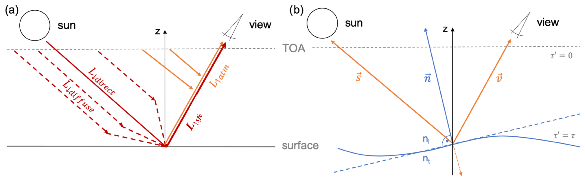
Figure A1 Sketches of the simple clear-sky model. (a) The main radiance components and (b) the geometry setup based on the vectors s pointing into the Sun, v pointing to the sensor, and the wave facet normal n.

The cloud-free radiance L reaching a sensor in space is a combination of three main components that we illustrate in Fig. A1a: (1) the direct sunray reflected at the ocean surface L_↓direct and (2) the hemispheric diffuse radiance reflected at the surface towards the sensor L_↓diffuse. Together they are combined in the component L_↑sfc of light that touched the surface. On the way from the surface to the sensor L_↑sfc experiences attenuation following Lambert–Beer and depending on the atmospheric optical thickness τ and the cosine of the sensor or view zenith angle v_z. In addition, there is component (3), the diffuse light from single-scattering events happening within the atmosphere L_↑atm.

$$\begin{array}{}\text{(A1)}& {\displaystyle }L& {\displaystyle }=L_{\uparrow \text{sfc}}+L_{\uparrow \text{atm}}\text{(A2)}& {\displaystyle }& {\displaystyle }=\exp \left({\displaystyle \frac{-\mathit{\tau }}{v_{\mathrm{z}}}}\right)\left[L_{\downarrow \text{direct}}+L_{\downarrow \text{diffuse}}\right]+L_{\uparrow \text{atm}}\end{array}$$

In the following, we describe the derivation of L based on the vector s pointing from an observed location on the ground to the Sun and the view vector v pointing to the sensor (see Fig. A1b).

$$\begin{array}{}\text{(A3)}& \mathit{s}=\left(\begin{array}{c}{s}_{\mathrm{x}}\\ s_{\mathrm{y}}\\ s_{\mathrm{z}}\end{array}\right)\text{, }\mathit{v}=\left(\begin{array}{c}{v}_{\mathrm{x}}\\ v_{\mathrm{y}}\\ v_{\mathrm{z}}\end{array}\right)\end{array}$$

s and v are unit vectors, meaning that they satisfy the condition

$$\begin{array}{}\text{(A4)}& \mid \mathit{s}\mid =\mid \mathit{v}\mid =\mathrm{1}.\end{array}$$

Working with vectors instead of the traditional approach with angles simplifies several of the following calculations next to a significant enhancement in computational speed. For example, the previously mentioned view zenith angle v_z is simply the third component of the view vector v.

A1 Direct radiance and the bidirectional reflection function (BRDF)

L_↓direct is defined by the sensor–Sun geometry with the cosine of the Sun zenith angle s_z and the corresponding aerosol extinction along the path from the top of the atmosphere (TOA) to the surface where the reflection is characterized by the bidirectional reflection function (BRDF) ρ.

$$\begin{array}{}\text{(A5)}& L_{\downarrow \text{direct}}=E_{\mathrm{0}}\exp \left({\displaystyle \frac{-\mathit{\tau }}{s_{\mathrm{z}}}}\right)\mathit{\rho }\left(\mathit{s},\mathit{v},\text{ws},n_{\mathrm{i}},n_{\mathrm{t}}\right)\end{array}$$

How a sunray is reflected at the ocean surface mostly depends on the surface wind speed “ws” and the generated wave slopes. The earliest and still widely used surface slope parameterization goes back to photographic measurements by Cox and Munk (1954). Their parameterization is embedded in a 1D Gaussian surface slope distribution p, combined with Fresnel reflection coefficients for unpolarized light r and a prefactor handling the sensor–Sun geometry with the Sun s and view v vectors. For the general equation for ρ we follow Stamnes et al. (2017).

$$\begin{array}{}\text{(A6)}& \begin{array}{rl}\mathit{\rho }(\mathit{s},\mathit{v},\text{ws},n_{\mathrm{i}},n_{\mathrm{t}})=& {\displaystyle \frac{\mathrm{1}}{\mathrm{4}{v}_{\mathrm{z}}{s}_{\mathrm{z}}(n_{\mathrm{z}}{)}^{\mathrm{4}}}}\cdot p(\mathit{s},\mathit{v},\text{ws})\\ & \cdot r(\mathit{s},\mathit{v},n_{\mathrm{i}},n_{\mathrm{t}})\end{array}\end{array}$$

In the first factor, n_z is the third component of the wave facet normal n with

$$\begin{array}{}\text{(A7)}& \mathit{n}=\left(\begin{array}{c}{n}_{\mathrm{x}}\\ n_{\mathrm{y}}\\ n_{\mathrm{z}}\end{array}\right)={\displaystyle \frac{\mathit{s}+\mathit{v}}{\mid \mathit{s}+\mathit{v}\mid }}.\end{array}$$

The second factor in Eq. (A6) gives the probability of a specular reflection p and the third the intensity of the reflected light r. In detail, we assume a 1D Gaussian surface slope probability distribution p with

$$\begin{array}{}\text{(A8)}& p(\mathit{s},\mathit{v},\text{ws})={\displaystyle \frac{\mathrm{1}}{\mathit{\pi }\mathit{\sigma }(\text{ws}{)}^{\mathrm{2}}}}\exp \left(-{\displaystyle \frac{\mathrm{1}-n_{\mathrm{z}}^{\mathrm{2}}}{n_{\mathrm{z}}^{\mathrm{2}}\cdot \mathit{\sigma }(\text{ws}{)}^{\mathrm{2}}}}\right),\end{array}$$

and the variance σ² of the surface slope distribution. The Cox and Munk parameterization provides an empirical estimate for σ² depending on the 10 m surface wind speed ws (Cox and Munk, 1954):

$$\begin{array}{}\text{(A9)}& \mathit{\sigma }(\text{ws}{)}^{\mathrm{2}}=\mathrm{0.003}+\mathrm{0.00512}\cdot \text{ws}.\end{array}$$

The intensity of the reflected light r is given by the unpolarized Fresnel reflection coefficient:

$$\begin{array}{}\text{(A10)}& r(\mathit{s},\mathit{v},n_{\mathrm{i}},n_{\mathrm{t}})={\displaystyle \frac{\mathrm{1}}{\mathrm{2}}}\left[{\left({\displaystyle \frac{{\mathit{\mu }}_{\mathrm{i}}-n_{\mathrm{r}}{\mathit{\mu }}_{\mathrm{t}}}{{\mathit{\mu }}_{\mathrm{i}}+n_{\mathrm{r}}{\mathit{\mu }}_{\mathrm{t}}}}\right)}^{\mathrm{2}}+{\left({\displaystyle \frac{{\mathit{\mu }}_{\mathrm{t}}-n_{\mathrm{r}}{\mathit{\mu }}_{\mathrm{i}}}{{\mathit{\mu }}_{\mathrm{t}}+n_{\mathrm{r}}{\mathit{\mu }}_{\mathrm{i}}}}\right)}^{\mathrm{2}}\right],\end{array}$$

with $n_r=\frac{n_{\mathrm{t}}}{n_{\mathrm{i}}}$, the ratio of the refractive index of the transmitted medium n_t=1.333 (ocean), and the refractive index of the incoming medium n_i=1 (atmosphere). Further, μ_i is the cosine of the incidence angle and is given by the dot product of the Sun and wave facet normal vector.

$$\begin{array}{}\text{(A11)}& {\mathit{\mu }}_{\mathrm{i}}=\mathit{s}\cdot \mathit{n}\end{array}$$

μ_t is the cosine of the transmission angle, which follows directly from Snell's law by transformation.

$$\begin{array}{}\text{(A12)}& {\mathit{\mu }}_{\mathrm{t}}=\sqrt{\mathrm{1}-{\displaystyle \frac{\mathrm{1}-{\mathit{\mu }}_{\mathrm{i}}^{\mathrm{2}}}{n_{\mathrm{r}}^{\mathrm{2}}}}}\end{array}$$

A2 Diffuse downward radiance and hemispheric BRDF

The hemispheric diffuse radiance L_↓diffuse includes sunrays that are scattered within the atmosphere on their way to the ground and get reflected at the pixel of interest in the direction of the sensor view. Thus, we integrate the integration vector x over the hemisphere Ω.

$$\begin{array}{}\text{(A13)}& L_{\downarrow \text{diffuse}}=\underset{\mathrm{\Omega }}{\int }\mathit{\rho }(\mathit{x},\mathit{v},\text{ws})\cdot L_{\mathrm{in}}(\mathit{\tau },\mathit{x})d\mathit{x}\end{array}$$

Assuming that the incoming diffuse downward radiance L_in(τ,x) is isotropic, we can pull L_in out of the integral and derive a hemispheric BRDF by integrating Eq. (A6) over Ω. Here, we make use of the Gauss–Legendre quadrature to approximate the integral based on only a few nodes in the μ space while keeping high accuracy.

The diffuse downward irradiance, on the other hand, is difficult to approximate. Thus, we sample from a pre-calculated lookup table of diffuse downward irradiance for a range of Sun zenith angles and aerosol optical depths. The lookup table was calculated with the full radiative transfer model libRadtran for a sensor at the surface pointing up nadir and observing at ASTER's band 3 central wavelength of 807 nm (Mayer and Kylling, 2005; Emde et al., 2016). The input file defines a US Standard Atmosphere with default molecular absorption calculated with the representative wavelength parameterization REPTRAN (medium) with the absorption based on the HITRAN 2004 catalog. The aerosol species is set to be maritime tropical as defined by the OPAC package, and finally, the radiative transfer equation is solved with DISORT. We further use the bivariate spline approximation provided within the Python package SciPy (version 1.5.2) to interpolate over the output lookup table.

A3 Diffuse upward radiance from single-scattering events

The atmospheric diffuse scattering L_↑atm describes sunrays that are reflected within the atmosphere in the view direction of the sensor. We only consider single-scattering events as the aerosol optical depth over tropical ocean is mostly below or of the order of 0.1 and the probability of further scattering events is unlikely. The extinction within an atmospheric column is generally given by the integral over the extinction coefficients σ_ext,i in single atmospheric layers depending on their density (temperature) and particles. We simplify the problem by integrating over τ instead of the atmospheric path lengths with $\mathrm{d}l=\frac{\mathrm{d}z}{\cos \left(\mathit{\theta }\right)}$ of a respective zenith angle θ. Correspondingly, we can write the integral over all single-scattering (aerosol) events along an atmospheric path l from the surface to TOA.

$$\begin{array}{}\text{(A14)}& {\displaystyle }{L}_{\uparrow \text{atm}}=E_{\mathrm{0}}\underset{\mathrm{sfc}}{\overset{\mathrm{TOA}}{\int }}& {\displaystyle }\exp \left(-{\displaystyle \frac{\mathrm{1}}{s_{\mathrm{z}}}}\underset{z_{\mathrm{scat}}}{\overset{\mathrm{TOA}}{\int }}{\mathit{\sigma }}_{\mathrm{ext}}\left(z\right)\mathrm{d}z\right)\text{(A15)}& {\displaystyle }& {\displaystyle }\cdot \exp \left(-{\displaystyle \frac{\mathrm{1}}{v_{\mathrm{z}}}}\underset{z_{\mathrm{scat}}}{\overset{\mathrm{TOA}}{\int }}{\mathit{\sigma }}_{\mathrm{ext}}\left(z\right)\mathrm{d}z\right)\text{(A16)}& {\displaystyle }& {\displaystyle }\cdot {\mathit{\sigma }}_{\mathrm{scat}}{\mathrm{\Theta }}_{\mathrm{HG}}\mathrm{d}{z}_{\mathrm{scat}}\end{array}$$

The extinction is accounted for in the exponential functions with the scattering event happening at the height z_scat. The product of the scattering coefficient σ_scat and the scattering phase function Θ_HG describes the scattering efficiency.

In our atmospheric column of constant density, σ_scat is independent of height and the integral ${\int }_{\mathrm{sfc}}^{\mathrm{TOA}}{\mathit{\sigma }}_{\mathrm{scat}}l\mathrm{d}l$ simplifies to ${\int }_{\mathrm{0}}^{\mathit{\tau }}\mathrm{d}{\mathit{\tau }}^{\prime }$ with τ being the optical depth of the atmospheric column. In more detail, we can rewrite the relation and include the single-scattering albedo ω₀,

$$\begin{array}{}\text{(A17)}& {\mathit{\sigma }}_{\mathrm{scat}}\cdot \mathrm{d}l={\mathit{\omega }}_{\mathrm{0}}{\mathit{\sigma }}_{\mathrm{ext}}\cdot {\displaystyle \frac{\mathrm{d}z}{{\mathit{\mu }}_{\mathrm{v}}}}={\displaystyle \frac{{\mathit{\omega }}_{\mathrm{0}}}{{\mathit{\mu }}_{\mathrm{v}}}}\mathrm{d}\mathit{\tau },\end{array}$$

and further include those in Eq. (A14):

$$\begin{array}{}\text{(A18)}& L_{\uparrow \text{atm}}={\mathrm{\Theta }}_{\mathrm{HG}}{\displaystyle \frac{{\mathit{\omega }}_{\mathrm{0}}}{{\mathit{\mu }}_{\mathrm{v}}}}\underset{\mathrm{0}}{\overset{\mathit{\tau }}{\int }}\exp \left({\displaystyle \frac{-{\mathit{\tau }}^{\prime }}{{\mathit{\mu }}_{\mathrm{o}}}}\right)\exp \left({\displaystyle \frac{-{\mathit{\tau }}^{\prime }}{{\mathit{\mu }}_{\mathrm{v}}}}\right)\mathrm{d}{\mathit{\tau }}^{\prime }.\end{array}$$

The Henyey–Greenstein phase function Θ_HG is an approximation for the scattering phase function and only depends on the asymmetry parameter g, which is the mean cosine of the scattering angle calculated by integrating over the scattering phase function (Henyey and Greenstein, 1941).

$$\begin{array}{}\text{(A19)}& {\mathrm{\Theta }}_{\mathrm{HG}}={\displaystyle \frac{\mathrm{1}}{\mathrm{4}\mathit{\pi }}}{\displaystyle \frac{\mathrm{1}-g^{\mathrm{2}}}{\mathrm{1}+g^{\mathrm{2}}-\mathrm{2}g{\left({\mathit{\mu }}_{\mathrm{scat}}\right)}^{\mathrm{3}/\mathrm{2}}}}\end{array}$$

For ω₀ and g we use constant values taken from the libRadtran calculations with the input setup described in Sect. A2.

Appendix B: Derivation of the cloud-free fraction

Based on Eqs. (6) and (7) we could directly solve for the cloud-free fraction p(F_CLEAR).

We start with the cloud-free model output and apply Bayes' theorem.

$$\begin{array}{}\text{(B1)}& p\left(F_{\mathrm{CLEAR}}\right|R)={\displaystyle \frac{p\left(R\right|F_{\mathrm{CLEAR}})}{p\left(R\right)}}\cdot p(F_{\mathrm{CLEAR}})\end{array}$$

We can add this information to Eq. (7),

$$\begin{array}{}\text{(B2)}& \mathrm{1}-p\left(F_{\mathrm{CLOUD}}\right|R^{\prime })={\displaystyle \frac{p(R=R^{\prime }|F_{\mathrm{CLEAR}})}{p(R=R^{\prime })}}\cdot p(F_{\mathrm{CLEAR}}),\end{array}$$

and solve for p(F_CLEAR).

$$\begin{array}{}\text{(B3)}& p\left(F_{\mathrm{CLEAR}}\right)={\displaystyle \frac{p(R=R^{\prime })}{p(R=R^{\prime }|F_{\mathrm{CLEAR}})}}(\mathrm{1}-p(F_{\mathrm{CLOUD}}\left|R^{\prime }\right))\end{array}$$

We further add the information from Eqs. (B1) and (B3) to our constraint stated in Eq. (6).

$$\begin{array}{}\text{(B4)}& {\displaystyle }\mathrm{1}\ge & {\displaystyle }p\left(F_{\mathrm{CLEAR}}\right|R)+p(F_{\mathrm{CLOUD}}\left|R\right)\text{(B5)}& {\displaystyle }\begin{array}{rl}\mathrm{1}\ge & {\displaystyle \frac{p\left(R\right|F_{\mathrm{CLEAR}})}{p\left(R\right)}}\cdot {\displaystyle \frac{p(R=R^{\prime })}{p(R=R^{\prime }|F_{\mathrm{CLEAR}})}}\\ & \cdot (\mathrm{1}-p(F_{\mathrm{CLOUD}}\left|R^{\prime }\right))\end{array}\text{(B6)}& {\displaystyle }& {\displaystyle }+p\left(F_{\mathrm{CLOUD}}\right|R)\end{array}$$

Rearranging the equation, we get

$$\begin{array}{}\text{(B7)}& {\displaystyle }& {\displaystyle \frac{p(R=R^{\prime \prime })}{p(R=R^{\prime \prime }|F_{\mathrm{CLEAR}})}}(\mathrm{1}-p(F_{\mathrm{CLOUD}}\left|R^{\prime \prime }\right)),\text{(B8)}& {\displaystyle }& {\displaystyle }\ge {\displaystyle \frac{p(R=R^{\prime })}{p(R=R^{\prime }|F_{\mathrm{CLEAR}})}}(\mathrm{1}-p(F_{\mathrm{CLOUD}}\left|R^{\prime }\right))\forall R^{\prime \prime }\in R,\end{array}$$

and consequently we can find R^′ by searching for the minimum.

$$\begin{array}{}\text{(B9)}& \begin{array}{rl}{R}^{\prime }& ={\text{argmin}}_{R^{\prime \prime }}\left({\displaystyle \frac{p(R=R^{\prime \prime })}{p(R=R^{\prime \prime }|F_{\mathrm{CLEAR}})}}\right.\\ & \left.-(\mathrm{1}-p(F_{\mathrm{CLOUD}}\left|R^{\prime \prime }\right))\right)\end{array}\end{array}$$

Knowing the R^′ we could in principle derive the cloud-free fraction p(F_CLEAR) from Eq. (B3). However, Eq. (B9) becomes unstable when $p\left(F_{\mathrm{CLOUD}}\right|R^{\prime \prime })$ is close to 1, which corresponds to cloudy parts, while we are interested in the clear part of the distribution. We therefore apply the modified method described in Sect. 3.2 in the current study.