Improved estimation of volcanic SO₂ injections from satellite retrievals and Lagrangian transport simulations: the 2019 Raikoke eruption

Monitoring and modeling of volcanic plumes are important for understanding the impact of volcanic activity on climate and for practical concerns, such as aviation safety or public health. Here, we apply the Lagrangian transport model Massive-Parallel Trajectory Calculations (MPTRAC) to estimate the SO₂ injections into the upper troposphere and lower stratosphere by the eruption of the Raikoke volcano (48.29^∘ N, 153.25^∘ E) in June 2019 and its subsequent long-range transport and dispersion. First, we used SO₂ retrievals from the AIRS (Atmospheric Infrared Sounder) and TROPOMI (TROPOspheric Monitoring Instrument) satellite instruments together with a backward trajectory approach to estimate the altitude-resolved SO₂ injection time series. Second, we applied a scaling factor to the initial estimate of the SO₂ mass and added an exponential decay to simulate the time evolution of the total SO₂ mass. By comparing the estimated SO₂ mass and the mass from TROPOMI retrievals, we show that the volcano injected 2.1 ± 0.2 Tg SO₂, and the e-folding lifetime of the SO₂ was about 13 to 17 d. The reconstructed SO₂ injection time series are consistent between using the AIRS nighttime and the TROPOMI daytime products. Further, we compared forward transport simulations that were initialized by AIRS and TROPOMI SO₂ products with a constant SO₂ injection rate. The results show that the modeled SO₂ change, driven by chemical reactions, captures the SO₂ mass variations from TROPOMI retrievals. In addition, the forward simulations reproduce the SO₂ distributions in the first ∼10 d after the eruption. However, diffusion in the forward simulations is too strong to capture the internal structure of the SO₂ clouds, which is further quantified in the simulation of the compact SO₂ cloud from late July to early August. Our study demonstrates the potential of using combined nadir satellite retrievals and Lagrangian transport simulations to further improve SO₂ time- and height-resolved injection estimates of volcanic eruptions.

1 Introduction

Injections of trace gases and ash by volcanic eruptions pose significant influences on the Earth's environment. Air pollutants such as sulfur dioxide (SO₂), released by volcanic eruptions, can lead to a severe public health hazard and increase excess mortality (Schmidt et al., 2011). In addition, volcanic ash and gases can directly interrupt air flights passing through the volcanic plume and cause long-term damage to airplanes through physical and chemical corrosion, such as sulfidation due to SO₂ (e.g., Grégoire et al., 2018; Prata, 2009). Furthermore, volcanic injections can influence the Earth's climate system through changes of radiative forcing (e.g., Robock, 2000; Kremser et al., 2016). Explosive volcanic eruptions can inject a significant amount of SO₂ into the stratosphere, and oxidation of the SO₂ forms stratospheric sulfate aerosol particles. Due to the limited potential of dry and wet deposition in the stratosphere, and due to the small sedimentation velocities, the sulfate aerosol particles have long lifetimes on timescales from months to years. In summary, as a precursor of stratospheric sulfate aerosol, and being a good proxy for other volcanic injections such as volcanic ash, monitoring and modeling of the injections and dispersion of volcanic SO₂ can help to better understand the impacts of volcanic eruptions.

Although in situ observations are available for several well-studied volcanoes (e.g., Whitty et al., 2020), remote-sensing measurements from satellite instruments are more suited to provide long-term records and retrievals on a global scale. At present, there are several satellite instruments that can provide SO₂ retrievals. Among them, the Atmospheric Infrared Sounder (AIRS) (Aumann et al., 2003; Chahine et al., 2006) aboard the National Aeronautics and Space Administration's (NASA) Aqua satellite provides retrievals of SO₂ in the upper troposphere–lower stratosphere (UTLS) region (e.g., Carn et al., 2005; Prata and Bernardo, 2007; Hoffmann et al., 2014). AIRS observations have been available since 2002 and have near-global coverage during both day- and nighttime. The newly operational TROPOspheric Monitoring Instrument (TROPOMI) aboard the Sentinel 5 Precursor (S5P) (Veefkind et al., 2012), which has been a cooperative undertaking between the European Space Agency (ESA) and the Kingdom of the Netherlands since late 2017, provides daytime SO₂ retrievals at an unprecedented spatial resolution (Theys et al., 2017, 2019), also covering the lower troposphere.

Beside the satellite retrievals, model simulations can help to characterize volcanic eruptions and provide forecasts of volcanic plume dispersion. In particular, Lagrangian particle dispersion models (LPDMs), which calculate air parcel trajectories following the fluid flow, are well suited for simulating complex transport processes (Lin et al., 2012). Widely used LPDMs include the Flexible Particle (FLEXPART) model (Stohl et al., 2005), the Hybrid Single-Particle Lagrangian Integrated Trajectory (HYSPLIT) model (Draxler and Hess, 1998), the Lagrangian Analysis Tool (LAGRANTO) (Wernli and Davies, 1997), the Numerical Atmospheric-dispersion Modeling Environment (NAME) (Jones et al., 2007), and the Stochastic Time-Inverted Lagrangian Transport model (Lin et al., 2003). A new LPDM, the Massive-Parallel Trajectory Calculations (MPTRAC) model, was recently developed at the Jülich Supercomputing Centre to take advantage of computing resources on state-of-the-art supercomputers (Hoffmann et al., 2016, 2022). The MPTRAC model has been successfully used to reconstruct volcanic SO₂ injections (Heng et al., 2016; Hoffmann et al., 2016) and simulate the long-range transport of volcanic SO₂ (Wu et al., 2017, 2018).

When simulating volcanic eruptions, suitable injection parameters, including the location, timing, and injection rate, are needed to initialize the LPDM simulations. Despite the importance of an accurate and reliable transport simulation, however, obtaining an accurate description of the injection parameters is challenging. Due to limited information regarding the injection parameters, the simplest assumption is a constant injection over the volcano (e.g., Muser et al., 2020; Kloss et al., 2021). However, uncertainties in the injection parameters can lead to errors in model simulations and consequently conflicting conclusions for a single volcanic eruption (Fromm et al., 2014). Complex modeling techniques using inversion algorithms and data assimilation have been developed to estimate volcanic injections (Eckhardt et al., 2008; Kristiansen et al., 2010; Flemming and Inness, 2013; Heng et al., 2016). In addition, the injection parameters can also be estimated based on backward trajectories (Hoffmann et al., 2016; Wu et al., 2017, 2018). The study of Heng et al. (2016) showed that forward transport simulation results using initialization strategies based on inverse modeling and the backward trajectory method may have comparable quality. Both the inverse modeling and backward trajectory methods considered here only give estimates of the altitude distribution and timing of volcanic injections. The SO₂ mass of air parcels in the altitude- and time-resolved space is assigned using a prior assumption of the total mass of SO₂ injections, which is usually estimated from satellite products. However, estimates of total SO₂ mass can be very different from study to study. For instance, the estimation of total SO₂ mass from the 2009 Sarychev eruption from different studies varies from 0.8 to 1.5 Tg (Fromm et al., 2014).

Several limitations may exist when using satellite products to estimate total SO₂ mass from volcanic eruptions. Large uncertainties exist during the initial stage of volcanic eruptions. The high SO₂ concentration in the early plume leads to saturation effects in satellite retrievals and, subsequently, an underestimation of the total mass. In addition, the co-presence of volcanic ash may also hamper the SO₂ mass retrieval at the early stage of an eruption (Yang et al., 2010). Although there is higher confidence after the initial stage, the conversion process of SO₂ to sulfate aerosol starts immediately after injection. Therefore, the SO₂ total mass burden retrieved by the satellite at a later stage, when the plume is dispersed and the ash sedimented out, also tends to underestimate the total SO₂ injection. In addition, the SO₂ is often not injected by the volcano at a single time during the initial stage, which further complicates the estimation of the total injected SO₂ mass.

The Raikoke volcano (48.29^∘ N, 153.25^∘ E) in the central Kuril Islands erupted during June 2019, sending a particularly large amount of ash and SO₂ into the UTLS (Hedelt et al., 2019; Muser et al., 2020; de Leeuw et al., 2021; Horváth et al., 2021). It was estimated that the 2019 Raikoke eruption injected 1.5 ± 0.2 Tg SO₂ into the atmosphere (Global Volcanism Program, 2019; Muser et al., 2020; de Leeuw et al., 2021), making it the largest SO₂ injection into the UTLS since the 2011 Nabro eruption and the first large volcanic eruption since the beginning of operations of TROPOMI. Interestingly enough, the Raikoke eruption formed unique features of compact SO₂ clouds with confined shapes and sizes (∼300 km in diameter) during the transport and dispersion of the SO₂ injections (Chouza et al., 2020; Gorkavyi et al., 2021). Therefore, the 2019 Raikoke eruption provides an ideal test case to assess the ability to reconstruct the injection parameters using the state-of-the-art TROPOMI SO₂ retrievals and to test how the reconstruction compares with retrievals using the older AIRS instrument. In addition, the compact SO₂ cloud phenomenon related to the Raikoke eruption provides a unique opportunity to test the simulation of the transport and dispersion of the volcanic SO₂. In this study, both questions are addressed.

The paper is structured as follows. In Sect. 2, we describe the satellite products of AIRS and TROPOMI and the MPTRAC model, as well as our method of reconstructing the injection parameters. The reconstructed injection parameters are presented in Sect. 3.1. In Sect. 3.2, we assess the performance of the MPTRAC model in simulating the transport and dispersion of the injected SO₂ in terms of the total mass of the volcanic SO₂, the spatial distribution of the SO₂ cloud, and the degree of dispersion of the compact SO₂ clouds. Finally, in Sect. 4 we discuss the results from our work through a comparison to previous studies, and main conclusions are drawn in Sect. 5.

2 Data and methods

2.1 AIRS SO₂ retrievals

To estimate the injection parameters of volcanic SO₂ and to initialize and validate the forward simulations with MPTRAC, we use SO₂ retrievals from AIRS and TROPOMI. Since May 2002, AIRS/Aqua has operated on a polar sun-synchronous orbit with an equatorial crossing time of 01:30 local time (LT) for the descending orbit and 13:30 LT for the ascending orbit. The scan for each swath covers a width of 1780 km, consisting of 90 footprints, and the along-track distance of two adjacent swaths is 18 km. The sizes of the footprints are 13.5 km × 13.5 km at nadir and 41 km × 21.4 km at the scan extremes.

AIRS measures thermal infrared spectra in three bands between 3.74 and 15.4 µm. For the SO₂ detection, we used the SO₂ index (SI) defined by Hoffmann et al. (2014), which identifies the brightness temperature difference (BTD) between two different radiance channels (1407.2 and 1371.5 cm⁻¹) from the AIRS spectral measurements in the 7.3 µm SO₂ waveband. The SI provides SO₂ information for the atmospheric column, but no vertical profile is directly available. The kernel function (Fig. 1) for the SI, based on radiative transfer calculations for a midlatitude atmosphere (Hoffmann et al., 2014), shows that the SI is most sensitive to SO₂ layers at 8 to 13 km. The SI is measured in units of kelvin and increases with increasing SO₂ column density. Here, we used a correlation function derived from the radiative transfer calculations of Hoffmann et al. (2014) for a midlatitude atmosphere to convert the SI to SO₂ column density. Based on our inspection of the AIRS data, measurements beyond a threshold of 1.4 K or 5 Dobson units (DU) are clearly indicating the presence of volcanic SO₂ from the 2019 Raikoke eruption. However, due to the conversion using an approximate correlation function, our estimates of total SO₂ mass from AIRS are generally considered to be less reliable, and total SO₂ mass will rather be obtained from the TROPOMI products in this study.

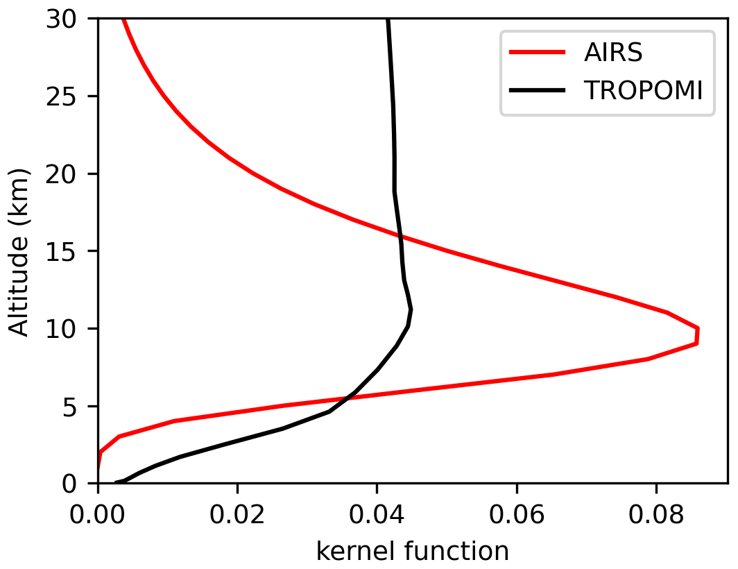
Figure 1 Representative kernel functions for AIRS SO₂ retrievals at midlatitudes and for TROPOMI SO₂ retrievals over the Raikoke region.

As an example, Fig. 2 shows plots of the Raikoke SO₂ clouds on 26 June 2019 as retrieved from AIRS (nighttime and daytime data, respectively) and TROPOMI (daytime data only) observations. Besides differences caused by the ∼12 h time shift, we found that the AIRS nighttime and daytime products were not always consistent with each other. They also showed some differences when reconstructing the Raikoke injection parameters. Therefore, the AIRS nighttime and daytime data are considered separately in this study.

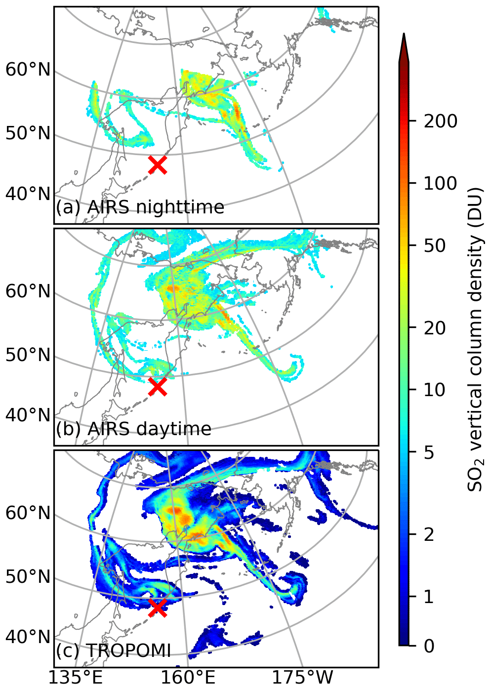
Figure 2 Spatial distribution of SO₂ vertical column density (DU) during the 24 h period between 26 June 2019, 12:00 UTC, and 27 June 2019, 12:00 UTC, from AIRS nighttime (a), AIRS daytime (b), and TROPOMI daytime (c) retrievals. Note that AIRS retrievals of SO₂ vertical column density less than 5 DU are not shown here as those data are not actually used in the analysis because they are affected by background noise. The AIRS nighttime retrievals have a ∼12 h time shift compared with the AIRS daytime and TROPOMI retrievals.

2.2 TROPOMI SO₂ retrievals

The TROPOspheric Monitoring Instrument (TROPOMI) is a single instrument on ESA's Copernicus Sentinel-5 Precursor satellite that was launched in October 2017. Sentinel-5P's mean local solar time of the ascending node is 13:30, and its orbit is aligned with NASA's Suomi-NPP mission (approximately 5 min behind) to allow for synergistic use with Suomi NPP's cloud products (Veefkind et al., 2012). TROPOMI consists of four passive grating imaging spectrometers measuring in the UV, Vis, NIR, and SWIR (Veefkind et al., 2012) and, hence, provides daytime measurements only. TROPOMI is a nadir instrument with a swath width of 2600 km and a very high spatial resolution of 7 × 3.5 km² (until August 2019) (Veefkind et al., 2012; Romahn et al., 2021).

For the analysis of the Raikoke eruption we used the TROPOMI Level 2 offline (OFFL) V01.01.07 SO₂ data product for the time period between 20 June 2019 and 16 August 2019. The TROPOMI SO₂ data product provides four total vertical columns of SO₂ in moles per square meter, one for the total atmospheric column between the surface and the top of the atmosphere and three columns assuming an SO₂ layer at 1, 7, and 15 km altitude in the retrieval. The details of the retrieval are given in Theys et al. (2017, 2021). In studies investigating volcanic plumes, it is common to use the vertical column densities retrieved for distinct plume heights (e.g., Theys et al., 2019). In this study, we used the total vertical SO₂ column of the 15 km retrieval, as we considered it to provide the best approximation for the Raikoke eruption as in other studies (e.g., Muser et al., 2020; de Leeuw et al., 2021). Compared with AIRS, the lower detection limit for TROPOMI is 0.3 DU (Theys et al., 2021), and data below this threshold are discarded in this study.

2.3 The MPTRAC model

Massive-Parallel Trajectory Calculations (MPTRAC) is a Lagrangian particle dispersion model for the analysis of atmospheric transport processes in the troposphere and stratosphere (Hoffmann et al., 2016). It calculates particle trajectories by solving the kinematic equation of motion using given wind fields from reanalysis or forecast meteorological data. The MPTRAC model currently uses the midpoint method to solve the equation of motion, which gives the optimized balance between accuracy and computational efficiency (Rößler et al., 2018). Besides vertical motion driven by the vertical velocity (i.e., kinematic trajectories), the MPTRAC model provides options to constrain the pressure of the air parcels to either constant pressure (isobaric surface), constant density (isopycnic surface), potential temperature (isentropic surface), or pressure time series from balloon measurements (Hoffmann et al., 2017). In addition, the model also includes turbulent diffusion and subgrid-scale wind fluctuations to simulate the diffusion. The turbulent diffusion is described by fixed diffusivity coefficients. Following the FLEXPART model (Stohl et al., 2005), the MPTRAC model uses a constant horizontal diffusivity of 50 m² s⁻¹ for the troposphere and a vertical diffusivity of 0.1 m² s⁻¹ for the stratosphere as default values. Subgrid-scale wind fluctuations are simulated using the Langevin equation to add time-correlated stochastic perturbations to the trajectories. The subgrid-scale wind standard deviations are downscaled from the grid scale standard deviations using a default scaling factor of 40 % (Stohl et al., 2005). To investigate the effect of parameterizations of turbulent diffusion and subgrid-scale wind fluctuations on the simulated SO₂ dispersion for the Raikoke case, we varied the diffusivity and the scaling factor of the subgrid-scale variance separately. As the actual diffusivity can vary by several orders of magnitude (e.g., Ishikawa, 1995; Desiato et al., 1998; Legras et al., 2005; Pisso et al., 2009), we tested the turbulent diffusion by varying the diffusivities from 10⁻² to 10³ times the default values. For subgrid-scale wind fluctuations, we varied the scaling factor from 0 % to 100 %.

Additional modules are implemented to simulate convection, sedimentation, radioactive decay, hydroxyl chemistry, dry deposition, and wet deposition. In this study, we used the hydroxyl chemistry module to simulate the loss of SO₂ by its reaction with the hydroxyl radical (OH). The MPTRAC model also provides variable output methods. In this study, we implemented a new module for “sample output”, which allows us to sample the model data at the exact time and location of the satellite overpasses/footprints. In addition to the trajectory and gridded outputs, the model also provides ways to directly evaluate the performance of the simulations, such as calculating the critical success index (CSI) (Wilks, 2011). Basically, the CSI is based on the counts of detection by the satellite retrieval and simulation on a regular grid basis. If the vertical column density in a grid cell passed a user-specified threshold, it will be counted as “yes”; otherwise it will be counted as “no”. The CSI is the ratio between the count of hits and the total number of hits, false alarms, and misses. Along with CSI, the probability of detection (POD) and the false alarm rate (FAR) are also calculated.

In this study, the main meteorological data used to drive the MPTRAC simulations are taken from the ERA5 reanalysis. The ERA5 is the ECMWF's (European Centre for Medium-Range Weather Forecasts) fifth-generation reanalysis (Hersbach et al., 2020), which is meant to replace its predecessor ERA-Interim (Dee et al., 2011). ERA5 provides hourly outputs of a comprehensive set of variables at a 31 km horizontal resolution and 137 vertical levels spanning from the surface up to 0.01 hPa. In this study, the ERA5 data are interpolated to a $\mathrm{0.3}{}^{\circ }\times \mathrm{0.3}{}^{\circ }$ horizontal resolution. In comparison, the ERA-Interim data have a horizontal resolution of 80 km, 60 model levels, and output every 6 h, i.e., at 00:00, 06:00, 12:00, and 18:00 UTC. The differences between ERA5 and ERA-Interim in driving Lagrangian transport simulations have been assessed by Hoffmann et al. (2019), finding that the choice of data has a considerable impact on the simulations, in particular due to better spatial and temporal resolutions of the ERA5 data. We also considered both ERA5 and ERA-Interim data in this study, with a major focus on results derived from the ERA5 reanalysis.

2.4 Estimation of volcanic SO₂ injections

To reconstruct the altitude- and time-resolved injection parameters of the Raikoke eruption, being represented by the altitude, time, and SO₂ mass of each air parcel over the volcano, we used a method based on backward trajectories released from the columns of the AIRS and TROPOMI SO₂ measurements (Hoffmann et al., 2016; Wu et al., 2017, 2018). The analysis was done separately for AIRS and TROPOMI data, covering time periods from a few days up to weeks after the eruption, and the results were compared against each other. As both AIRS and TROPOMI provide information on the horizontal location and time of SO₂ retrievals but lack information on the vertical distribution of the SO₂, we released multiple air parcels between 0 and 25 km altitude at each individual satellite footprint with volcanic SO₂ detections. In contrast to our earlier work, the vertical profile of the number of air parcels has been made to follow the mean kernel function of the satellite measurements (Fig. 1) in order to take into account their different vertical sensitivity. The total number of air parcels at each location was linearly proportional to the total column density of the satellite retrievals. At the same time, a Gaussian scatter of the air parcels with 15 and 5 km full width at half maximum (FWHM) was introduced to represent the horizontal footprint size for AIRS and TROPOMI, respectively.

In total, 5 million air parcels were released to calculate backward trajectories. If a backward trajectory passed the Raikoke volcano within a search radius of 15 km, the location and time of the air parcel were saved to reconstruct the injection parameters. We note that, based on our sensitivity tests, the results are not very sensitive to FWHM (i.e., between 1 and 50 km) and the search radius around the volcano (i.e., between 1 and 100 km). However, it is possible that for a given TROPOMI pixel location, there may be multiple solutions in the backward trajectory method, especially if the wind does not change with height and over time. In the study, this uncertainty has been reduced through two ways. First, all TROPOMI overpasses over many days, in the final reconstruction 12 d, were used, and second, an increased number of particles, 5 million air parcels, were released in the backward run. All backward trajectories that met the selection condition were resampled to a total number of 5 million particles, and an initial total mass of 1.5 Tg was assigned to them. After the initial relative SO₂ distribution has been estimated from the backward trajectories, we conducted forward simulations and applied a scaling factor to the SO₂ total mass for further calibration. To calibrate the total mass, we assumed that the SO₂ starts to decay exponentially with a fixed e-folding lifetime, representing the overall removal of the SO₂, immediately after the injection and compared the change of the SO₂ total mass from the simulations with the change of the SO₂ total mass derived from TROPOMI retrievals.

3 Results

3.1 Volcanic SO₂ injections parameters

3.1.1 Final reconstruction of Raikoke SO₂ injections

Figure 3 shows the final reconstruction of the Raikoke SO₂ injections based on the TROPOMI SO₂ product and Lagrangian transport simulations using ERA5 winds. The mass in the reconstruction has been tuned to achieve a total injection of 2.1 Tg (see Sect. 3.1.2 for details on how the total mass was derived). The altitude- and time-resolved injection and the integrated vertical profile are also shown in Fig. 3. A major SO₂ injection was reconstructed during the first 2 d of the time series, i.e., between 21 and 22 June 2019. After this major eruption, significantly smaller amounts of SO₂ were continuously injected by the volcano until the end of June, with a prominent second and third plume during 24–25 June and 27–28 June, respectively. The first plume crossed the temperature lapse-rate tropopause (WMO, 1957) and injected SO₂ between 5 and 15 km of altitude, with ∼45 % of the SO₂ mass reaching the stratosphere (Fig. 3a and b). The second and the third plumes mainly injected material into the troposphere. As the Raikoke eruption is dominated by the first plume, the overall injected SO₂ (Fig. 3c) distributes around the tropopause, with peak injections at an altitude of 11 km.

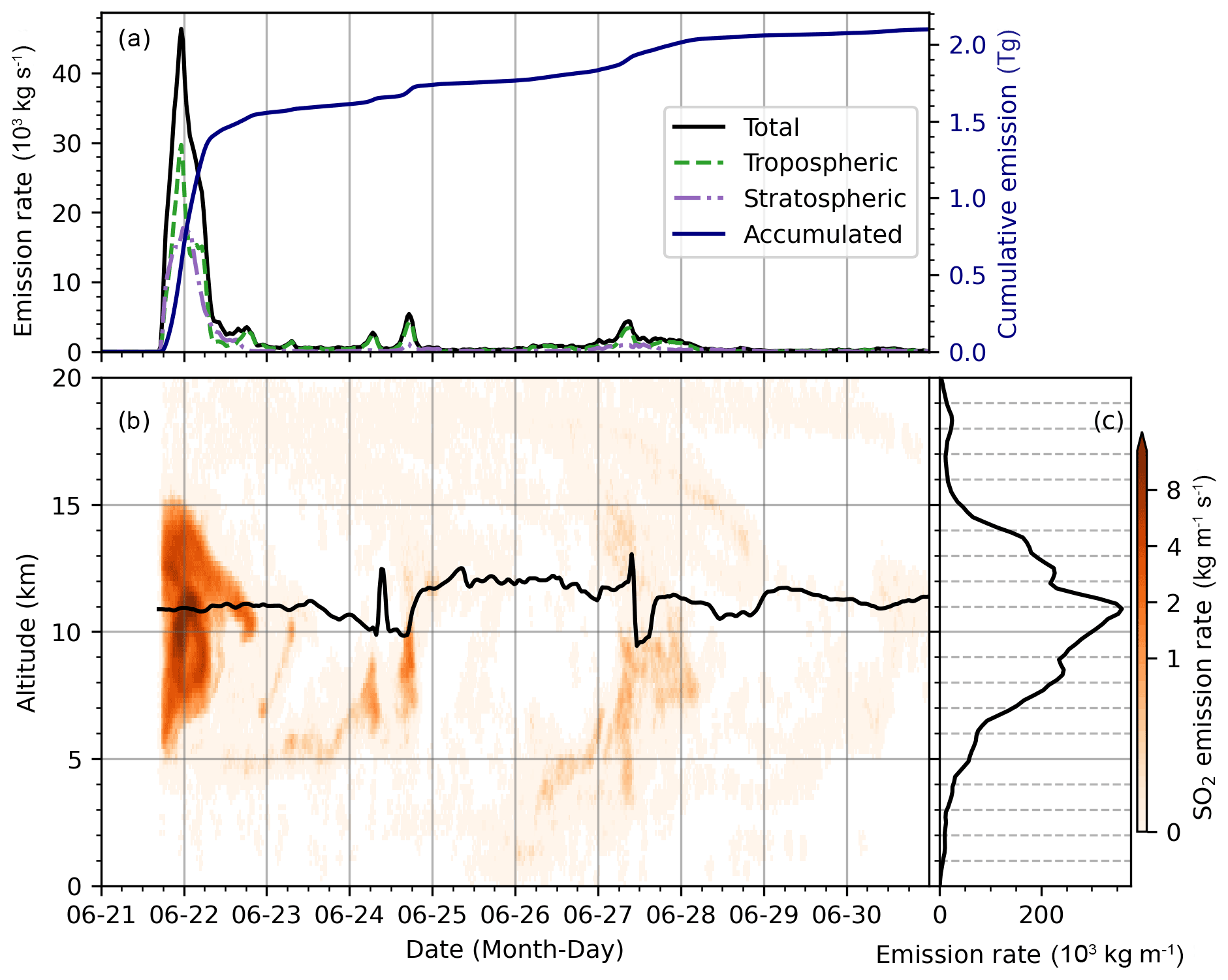
Figure 3 Reconstructed SO₂ injections of the 2019 Raikoke eruption based on the TROPOMI SO₂ product. (a) Temporal evolution of the vertically integrated SO₂ injection rates (kg s⁻¹) for the whole atmosphere, the troposphere, and the stratosphere. The temporal change of accumulated SO₂ injections (integrated for the whole atmospheric column and over time) is also plotted in (a). (b) Altitude-resolved SO₂ injection rate time series (kg m⁻¹ s⁻¹). The black line represents the ERA5 temperature lapse-rate tropopause (WMO, 1957) over the Raikoke volcano. (c) Altitude profile of the SO₂ injection rates (kg m⁻¹).

As an intercomparison as well as a validation, the vertical profiles integrated over the entire eruption period (21–30 June 2019) of our different injection estimations and the profile derived by the VolRes team (de Leeuw et al., 2021) are shown in Fig. 4. The profile derived by the VolRes team is mainly based on IASI retrievals during the first 2 d of the Raikoke eruption (de Leeuw et al., 2021). Compared with the VolRes profile, the altitude of peak injections is about 1 km above the VolRes profile, no matter which satellite data, i.e., AIRS nighttime or TROPOMI daytime, and reanalysis data, i.e., ERA5 or ERA-Interim, have been used. Our reconstructions also show enhanced injections between 12 and 14 km, being consistent with de Leeuw et al. (2021) that the injections reached higher into the stratosphere than indicated by the VolRes estimation. When excluding the second and third plume, the vertical profile for the first major eruption (figure not shown) is similar to the overall injection profile (Fig. 4), with a slightly reduced injection rate in the stratosphere and a larger reduction in the tropospheric part. The VolRes profile also indicates a small peak at low altitudes around 2 km. However, this part is not found in our reconstruction. The most likely reason is that both AIRS and TROPOMI have a limited sensitivity in the lower troposphere, i.e., below 5 km (Fig. 1).

Figure 4 Vertical profiles of Raikoke SO₂ injections derived by the VolRes team and from different combinations of datasets (see plot legend).

3.1.2 Calibration of the total mass of the SO₂ injections

For the initial reconstruction, we estimated the SO₂ injection rates under the assumption of a SO₂ total mass of 1.5 Tg, as found by the VolRes team. Figure 5 shows the time series of the vertically integrated SO₂ injections. The comparison of the reconstructions based on different satellite SO₂ products (Fig. 5) shows that the results derived from AIRS nighttime and TROPOMI SO₂ products agree well. The reconstruction derived from the AIRS daytime SO₂ product shows weaker injections in the first plume, but the second and third plume are stronger compared to the reconstructions based on AIRS nighttime and TROPOMI SO₂ products. As pointed out in Sect. 2.1, we will focus our analyses on the AIRS nighttime and TROPOMI results in the following parts.

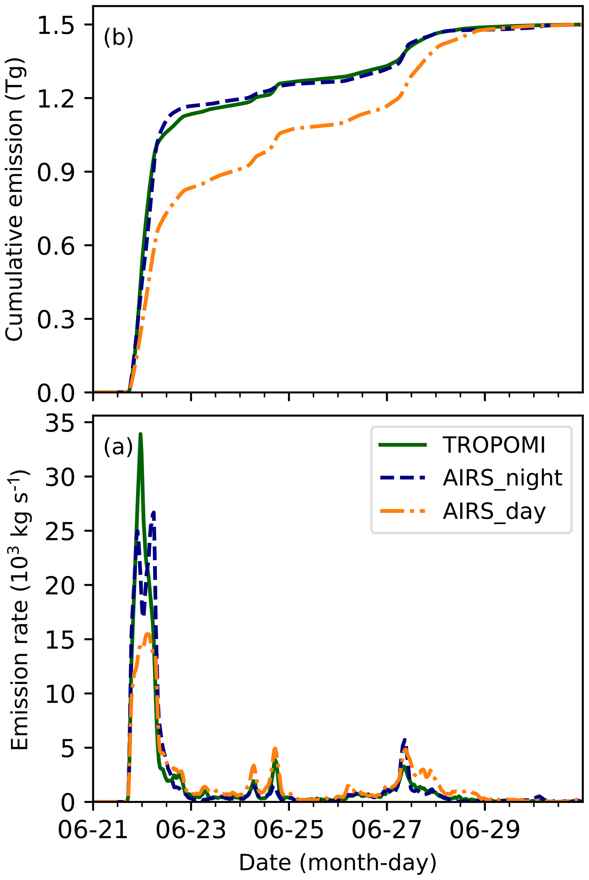
Figure 5 Temporal change of the Raikoke SO₂ injections reconstructed based on the TROPOMI SO₂ product (green line) and AIRS SO₂ product during nighttime (dashed blue line) and daytime (dashed–dotted orange line): (a) vertically integrated SO₂ injection rate and (b) accumulated SO₂ mass.

To estimate the final total injected SO₂ mass, we derived the daily SO₂ mass from the TROPOMI SO₂ product (Fig. 6). The TROPOMI SO₂ product shows that a total SO₂ mass of ∼1.4 Tg peaked during 24–26 June, while the cumulative SO₂ injection from the initial reconstruction at 26 June is only ∼1.2 Tg. When the cumulative SO₂ injection in the initial reconstruction reached 1.5 Tg, the total SO₂ mass from TROPOMI decreased to ∼1.2 Tg due to the removal of SO₂. To better represent the evolution of the total SO₂ mass in the simulations, we scaled our initial mass reconstruction to the TROPOMI data and applied an exponential decay to represent the overall removal of SO₂ (Fig. 6; Sect. 3.2.1 gives more detailed information on the lifetime). In this experiment, we found that a total injection of 1.9 to 2.3 Tg SO₂ and an e-folding lifetime of 13 to 17 d best represent the temporal evolution of total SO₂ mass in the atmosphere. Therefore, we rescaled the initial reconstruction to a total mass of 2.1 Tg. Note that although the e-folding lifetime of 13–17 d represents the overall removal of SO₂ injections for the Raikoke case well, SO₂ removal rates in general are very sensitive to the altitude of the SO₂ injections and the atmospheric background conditions.

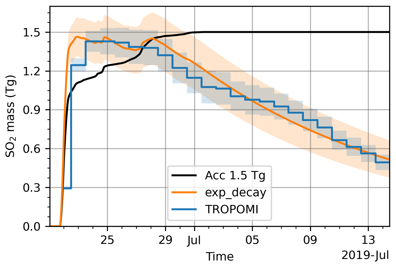
Figure 6 Temporal change of total SO₂ mass from TROPOMI measurements (blue) and calculated total mass with an e-folding lifetime of 15 d (orange) and a mass scaling factor of $\mathrm{2.1}/\mathrm{1.5}$. Orange shadings show the combination of the scaling factor ranging between $\mathrm{1.9}/\mathrm{1.5}$ and $\mathrm{2.3}/\mathrm{1.5}$ and an e-folding lifetime ranging between 13 and 17 d. The black curve shows the accumulated SO₂ injection with a total injection of 1.5 Tg (the initial reconstruction).

3.1.3 Sensitivities of estimated SO₂ injections to data and model parameters

To investigate the sensitivity of the reconstructed injection time series to the underlying input data, we ran the reconstruction using the AIRS SO₂ product together with ERA5 winds as well as the TROPOMI SO₂ product together with ERA-Interim winds. In comparison to TROPOMI and ERA5, the overall patterns of injection estimations based on AIRS nighttime observations and ERA5 (Fig. 7a) or TROPOMI observations and ERA-Interim (Fig. 7b) are quite similar. For the first plume, i.e., between 21 and 22 June, the estimation based on AIRS nighttime observations and ERA5 shows stronger injections during the beginning and late stage of the plume, while the estimation based on TROPOMI observations and ERA-Interim shows weaker (stronger) injections at the beginning (late) stage of the first plume, respectively. Differences do exist during the second and the third plumes, but they are relatively small.

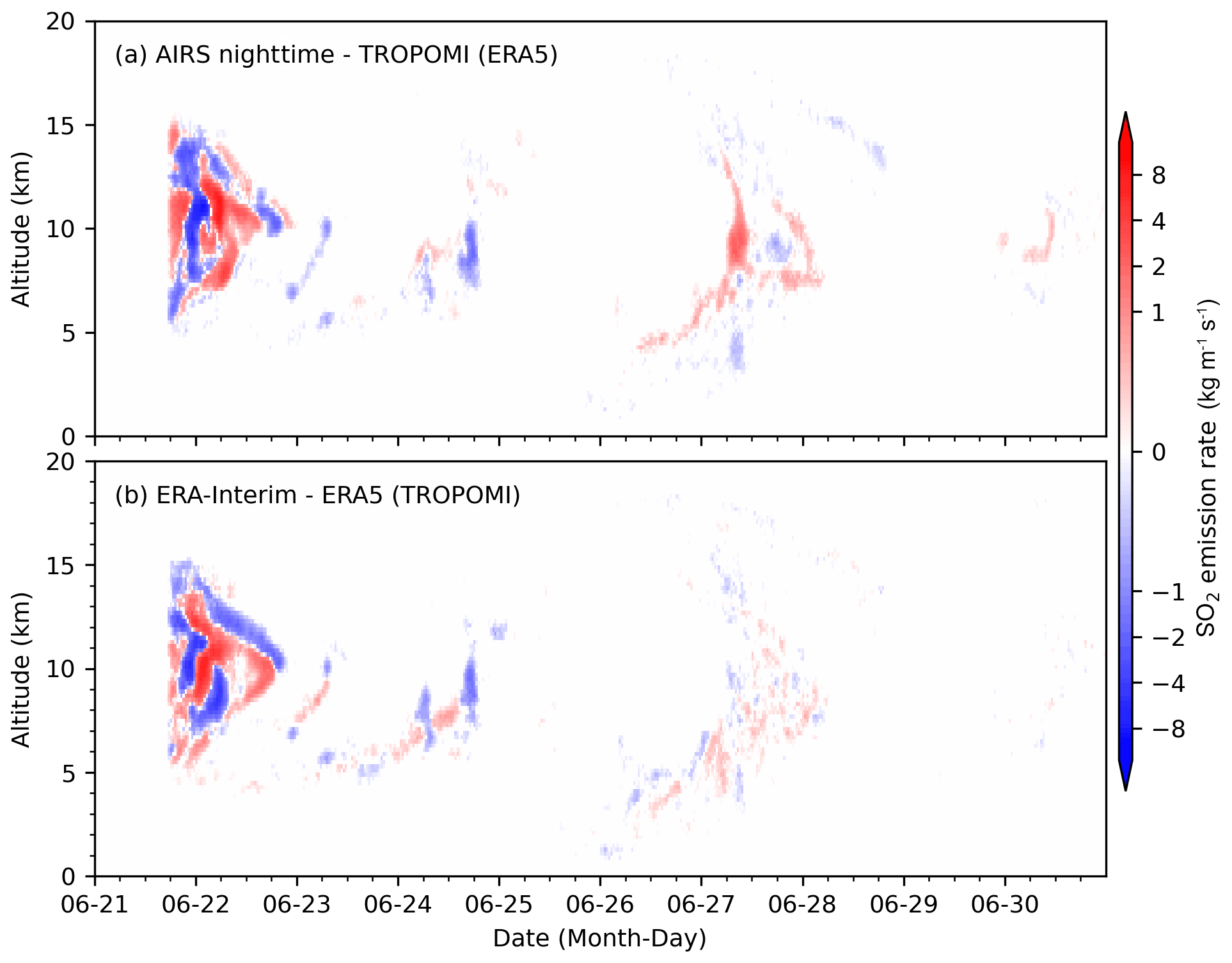
Figure 7 Differences in reconstructed SO₂ injections of the 2019 Raikoke eruption derived from different combinations of satellite products and reanalysis data compared with the TROPOMI-ERA5 combination: AIRS nighttime with ERA5 (a) and TROPOMI with ERA-Interim (b).

We conducted more than 200 simulations to test the sensitivity of the injection reconstructions. Among the tested parameters, we found that the coverage of the satellite observations has the largest impact on the injection reconstruction. More specifically, it matters how many days of satellite retrievals are used for the reconstruction and how close to the location of the volcano satellite retrievals are discarded. Here, we only describe the sensitivity tests on the temporal and spatial coverage of the satellite retrievals, whereas the sensitivity tests on other parameters are not shown.

Figure 8 shows the SO₂ mass change in forward simulations initialized using TROPOMI observations covering different numbers of days since the beginning of the eruption. The total SO₂ mass in all the simulations was assigned to 2.1 Tg. As shown in Fig. 8, when using just a few days of observations, the simulation produces too strong a peak at the beginning of the volcanic eruption. Increasing the time period of the satellite data, a gradual decrease of the first peak and redistribution of SO₂ to a later stage of the eruption is observed in the different forward simulations. Therefore, using short-term observations will lead to a more pronounced first plume, and conversely, longer-term observations will increase the amplitude of the second and third plume. The sensitivity test shows that using 12 d of observations gives an optimal representation of the SO₂ mass.

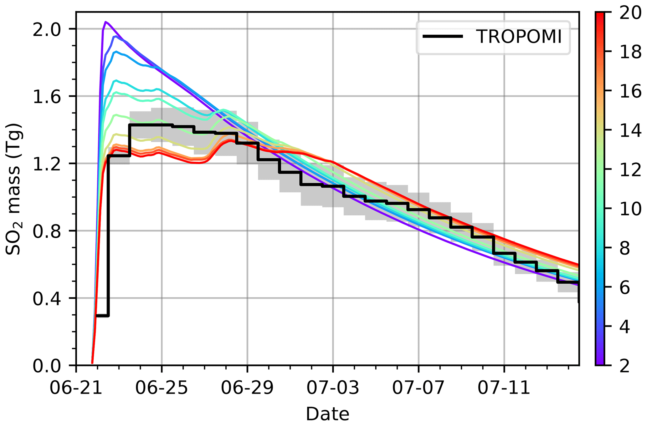
Figure 8 Temporal change of SO₂ total mass in MPTRAC forward simulations, which were initialized by considering different numbers of days of TROPOMI observations since the beginning of the Raikoke eruption (see color bar). Total mass of SO₂ injection in all simulations is 2.1 Tg. In the forward simulations, the mass is derived from the chemistry module. The mass changes measured by TROPOMI are shown by the black line, and gray shading indicates the measurement errors.

As the backward trajectory method heavily relies on the quality of the trajectories, satellite observations too close to the volcano can not provide enough information to separate between different altitudes. Therefore, we defined a circle with a certain distance to the Raikoke volcano, where the satellite observations falling inside the circle are discarded. When using the TROPOMI SO₂ product and the distance is set to a very small value, such as a few kilometers, most of the reconstructed SO₂ is injected at the beginning of the eruption. When the distance is set to several hundred kilometers, similar to increasing the temporal duration of the trajectories, the injection of SO₂ at the beginning of the eruption is weakened, and more SO₂ is injected within a few to several days after the beginning of the eruption. When using the AIRS product, this effect becomes less pronounced. Overall, the AIRS and TROPOMI reconstructions agreed better with each other when setting a larger distance. In the final reconstruction, we used a distance of 750 km, which gave the most consistent results.

3.2 Forward simulations for the Raikoke eruption

3.2.1 Simulations of SO₂ total mass

We performed forward simulations initialized by the different reconstructed SO₂ injection parameters as well as a constant SO₂ injection rate. For the forward simulation with a constant injection, we uniformly assigned 1.5 Tg SO₂, which is the initial estimate of the total SO₂ injection, from 5 to 15 km and from 21 June 2019, 18:00 UTC, to 22 June 2019, 06:00 UTC. Unless noted differently, all forward simulations that were initialized by a constant injection rate in the following sections have the same setup as described here. In addition, we also performed a forward simulation initialized by the VolRes profile with a total SO₂ injection of 1.5 Tg assigned between 21 June 2019, 18:00 UTC, and 22 June 2019, 06:00 UTC. In the following subsections, we will present and compare the forward simulations of SO₂ in terms of total mass burden and spatial distributions. In addition, we also performed different forward simulations driven by ERA5 and ERA-Interim data. However, the overall patterns of simulated SO₂ were generally similar between ERA5 and ERA-Interim. Therefore, if not specified otherwise, the forward simulations driven by the ERA5 data are shown.

In the most recent version of the MPTRAC model, a hydroxyl (OH) chemistry module has been implemented to simulate the removal of SO₂ due to the thermomolecular reaction with OH (Hoffmann et al., 2022). Monthly mean zonal mean OH concentrations are obtained from the study of Pommrich et al. (2014). This module enables the direct comparison of total SO₂ mass change in model simulations with the simple exponential decay experiments and the satellite product by TROPOMI (Fig. 9). In the forward simulations, we have used different injection parameters with total injected SO₂ mass ranging from 1.9 to 2.3 Tg. As shown in Fig. 9, the SO₂ mass in the forward simulation initialized with a 2.1 Tg total injection, either using injection parameters derived from TROPOMI daytime (Fig. 9a) or AIRS nighttime (Fig. 9b) observations, agrees well with the exponential decay experiment of a 15 d e-folding lifetime. In addition, all the experiments are consistent with the total SO₂ mass derived from TROPOMI SO₂ retrievals. Figure 9 also shows the SO₂ mass change in the forward simulation initialized by a constant injection time series. In contrast to the forward simulation initialized by our reconstructed injection time series, the simulation initialized with a constant injection rate or the VolRes profile produced an SO₂ mass peak, which is comparable with the maximum SO₂ mass in TROPOMI retrievals, at the beginning of the eruption. Then, the gradual removal of SO₂ leads to lower mass in the model simulation than TROPOMI retrievals (Fig. 9). From these comparisons, we conclude that the June 2019 Raikoke eruption produced a total injection of 2.1 Tg SO₂, which has an overall e-folding lifetime of 15 d in the UTLS region during the first 3 weeks after the eruption.

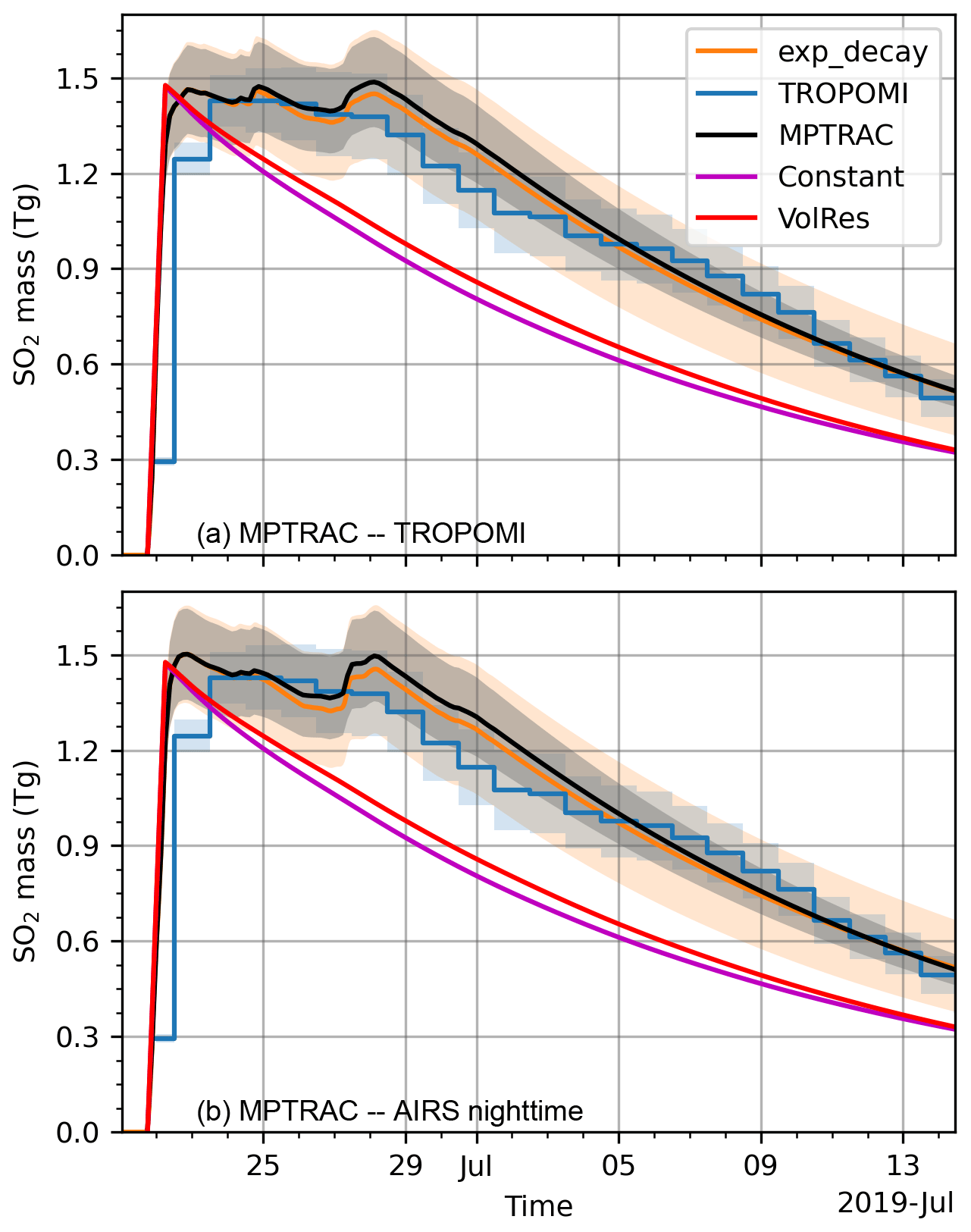
Figure 9 Temporal change of total SO₂ mass in the MPTRAC forward simulation (black lines) initialized by TROPOMI observations (a) and AIRS nighttime observations (b), respectively. Gray shadings show the range of total injection between 1.9 and 2.3 Tg. Temporal changes of total SO₂ mass in the MPTRAC forward simulations initialized by the VolRes profile (red) and a constant injection rate (magenta) of 1.5 Tg total injection are also plotted. In the forward simulations, the mass is derived from the chemistry module. The mass changes measured by TROPOMI (blue) and modeled by an exponential decay (orange) from Fig. 6 are repeated here for comparison.

The comparison of the temporal changes of the SO₂ total mass among the different forward simulation settings and TROPOMI retrievals (Fig. 9) suggests that our estimation of 2.1 Tg SO₂ injection is reasonable. The initial estimation of 1.5 Tg mainly reflects SO₂ injections of the major eruption during the first 2 d. Consistent with this estimate, the total mass in our estimation for the first plume is about 1.5 Tg (Fig. 3a). However, additional injections after the first plume are required to reproduce the retrieved SO₂ mass in the model simulations (Fig. 9).

Although an e-folding lifetime of 15 d captures the overall mass reduction of injected SO₂ in the atmosphere well, the real removal rates of SO₂ at different altitudes are different. Figure 10 shows the remaining mass of SO₂ injected to 1 km thick layers between 0–25 km during the first 12 h of the eruption (21 June 2019, 18:00 UTC to 22 June 2019, 06:00 UTC). In general, the removal rate decreases with altitude, mostly because of lower OH concentrations in the lower stratosphere compared to the troposphere. In the troposphere, the SO₂ mass is reduced to less than 50 % within several days to a week, while the stratospheric injections still have ∼70 % at 10 d after the eruption. This means that the tropospheric injections are removed quickly during the early stage of the eruption, and the stratospheric injections gradually dominate. In the satellite SO₂ retrievals, the vertical column density of the SO₂ cloud associated with the tropospheric injection also decreases faster than the SO₂ cloud associated with stratospheric injection (Fig. 11; see details below). This observation also confirms the faster removal of tropospheric parts of the SO₂ injections.

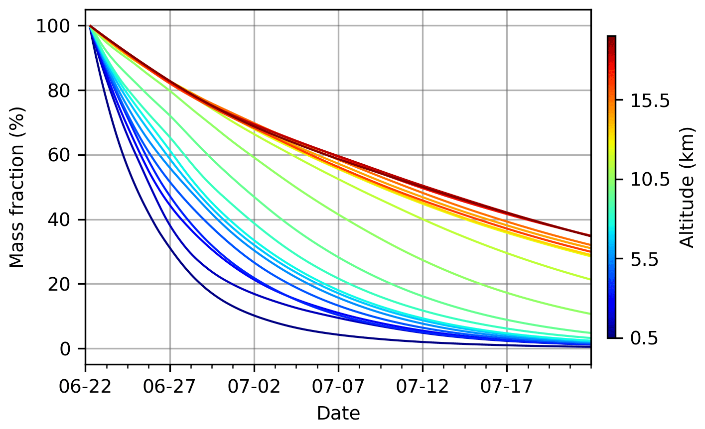
Figure 10 Temporal change of the remaining fraction of SO₂ mass for injections at different 1 km thick layers between 0 and 25 km and from 21 June 2019, 18:00 UTC, to 22 June 2019, 06:00 UTC. Colors indicate the altitude at the middle of each 1 km thick layer.

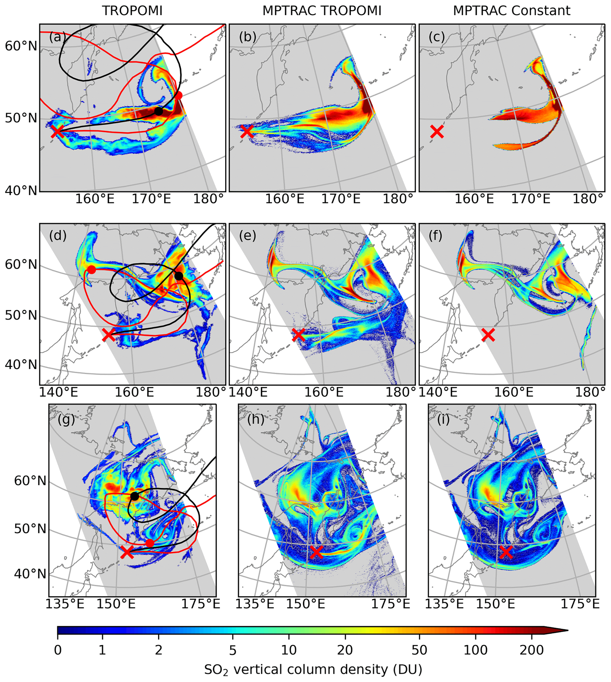
Figure 11 TROPOMI retrievals and MPTRAC forward simulations of SO₂ transport. Top row (a–c): spatial distribution of SO₂ vertical column density (DU) from the TROPOMI orbit that starts at 23 June 2019, 01:05 UTC, and ends at 23 June 2019, 02:47 UTC (a), and the corresponding distribution in forward simulations, which were initialized by TROPOMI retrievals (b) and by a constant injection rate (c), respectively. Middle and bottom rows show the same as the top row but for the orbits of 25 June 2019, 00:27–02:09 UTC, and 28 June 2019, 01:12–02:53 UTC, respectively. The mean trajectories for injections between 7–8 km (red curve) and 11–15 km (black curves) are plotted on the maps on the left, and the mean locations at the corresponding time of each map are indicated by red and black dots.

3.2.2 Simulation of SO₂ transport during the first ∼10 d

In general, the forward simulations initialized by both the TROPOMI daytime and AIRS nighttime SO₂ products reproduce the spatial distribution of SO₂ during the first ∼10 d of simulation time well, especially in terms of spatial location and extent. We note that the forward simulations initialized by the TROPOMI and AIRS nighttime products are highly consistent with each other, as the injection parameters estimated from these two datasets do not differ fundamentally (Fig. 7). Therefore, the results from the forward simulation initialized by the AIRS nighttime product are not shown here. As our forward simulations initialized by the VolRes profile are identical with the results presented by de Leeuw et al. (2021), SO₂ distributions in these simulations are not shown here. To illustrate the performance after major SO₂ injections of Raikoke, we selected three satellite overpasses on 23, 25, and 28 June to show the SO₂ distribution in retrievals and model simulations (Fig. 11).

The TROPOMI retrievals and the MPTRAC simulations show that the SO₂ injections are separated into two major clouds (Fig. 11). We added mean trajectories for injections between 7–8 and 11–15 km in Fig. 11 to indicate the major movements of the two SO₂ clouds. Both of the SO₂ clouds are moving cyclonically. A smaller SO₂ cloud, which is represented by the mean trajectory for injections between 7 and 8 km, moves faster, and the SO₂ column density also decreased very fast to less than 10 DU on 28 June. The SO₂ column density in the other major cloud, which mainly reflects the stratospheric injections, decreased much slower compared with the SO₂ cloud that reflects tropospheric injections. This observation by TROPOMI retrievals is consistent with the faster removal of SO₂ in the troposphere (Fig. 10).

After the first injection, the TROPOMI SO₂ product shows that the SO₂ clouds are located to the east of the Raikoke volcano but split into two branches, with one branch being in the north and the other branch being in the south (Fig. 11a). The forward simulations initialized by the TROPOMI retrievals and a constant injection rate reproduce the main northern branch, which is located just to the east of the Raikoke volcano (Fig. 11b and c). However, both simulations only reproduce a part of the southern branch and the part reproduced in the simulation initialized by a constant injection rate is too strong. Compared with the major northern branch SO₂ cloud, we find that the southern branch is very weak with SO₂ column densities mostly less than 10 DU. The much lower column density reduces the chance of identifying a source associated with this part of the SO₂ cloud. In addition, the TROPOMI averaging kernel significantly reduces the air parcels that started at altitudes below 5 km, which further reduces the chance of identifying a source at altitudes lower than 5 km. A sensitivity test suggested that the southern branch is mainly associated with transport of SO₂ in the lower troposphere (between 0 and 5 km), which was not represented in both initializations.

After the second plume on 25 June (Fig. 11d–f), most of the SO₂ injections were moved to the northwest direction over the Asian continent and to the northeast direction over the northwest Pacific Ocean (Fig. 11d). In addition to these two major SO₂ clouds, there is a weaker SO₂ cloud to the east of the Raikoke volcano, which is probably related to the injections between 23 and 25 June (Fig. 3). The forward simulation initialized by the TROPOMI SO₂ product reproduced the general pattern of the three clusters. However, the forward simulation initialized by a constant injection rate only reproduces the two major SO₂ clouds in the northwest and the northeast directions (Fig. 11f). Injections at lower altitudes from the VolRes profile could also partly explain the part not represented in Fig. 11f; however that part is also underestimated in the forward simulation initialized by the VolRes profile shown in de Leeuw et al. (2021).

After the third plume on 28 June (Fig. 11g), the SO₂ cloud that was located over the Asian continent in the northwest direction now moved back to the east of Raikoke along a cyclonic circulation. In contrast, the SO₂ cloud that was over the northwest Pacific Ocean showed a slower movement and is now located over the Asian continent (Fig. 11g). Both forward simulations reproduced the two major SO₂ clouds. The forward simulation initialized by the TROPOMI SO₂ product reproduced a stronger SO₂ cloud to the east of the Raikoke volcano (Fig. 11h) due to injections during the third plume. Similarly, the simulated SO₂ cloud over the volcano after the second plume is also stronger than in the satellite retrievals (Fig. 11e). This result indicates that our reconstructed injection parameters potentially overestimate the second and the third plume. However, totally removing the second and/or the third plume would severely reduce the ability to correctly simulate the total SO₂ mass burden as shown in Fig. 9.

Although the forward simulations can reproduce the retrieved SO₂ distributions with relatively high performance during the first week (Fig. 11), the simulation starts gradually losing the ability to capture the structures of the SO₂ cloud thereafter. Figure 12 shows the retrieved and simulated spatial distribution of SO₂ at the beginning of 1 July. Overall, the SO₂ distributes like a strip pattern with major peaks over the Sea of Okhotsk and the west coast of the Bering Sea (Fig. 12a). The model simulation captured this overall strip-like pattern and even some fine details over northern high latitudes (Fig. 12b). However, the simulated SO₂ distribution does not correctly reproduce the peaks over the Sea of Okhotsk and the west coast of the Bering Sea. Several days later, the retrieved SO₂ over the west coast of the Bering Sea gradually spreads out, and its vertical column density gradually attenuates (not shown). In contrast, the two SO₂ peaks over the Sea of Okhotsk retained their compact structures and relatively high vertical column density. From mid-July to late July, the two peaks over the Sea of Okhotsk eventually comprise the main parts of the remaining SO₂ of the Raikoke eruption and developed into two compact SO₂ clouds. As the simulated SO₂ did not reproduce the two peaks over the Sea of Okhotsk, however, the forward simulation lost its ability to capture the retrieved SO₂ distribution during the first week of July.

Figure 12 Spatial distribution of SO₂ vertical column density (DU) from the TROPOMI orbits that start at 1 July 2019, 00:15 UTC, and end at 1 July 2019, 03:38 UTC (a), and the corresponding distribution in the forward simulation, which was initialized by TROPOMI data (b). Note that data for the region in the east and west of 160^∘ E are from two neighboring orbits.

3.2.3 Assessment of forward simulations by means of the Critical Success Index

We performed analyses of the Critical Success Index (CSI) to evaluate the forward simulations at five different detection thresholds ranging from 0.3 to 50.0 DU (Fig. 13). Figure 13a–c show the CSI, POD, and FAR time series for the forward simulation initialized with the TROPOMI SO₂ product. The reference for calculating the CSI, POD, and FAR is also the TROPOMI retrievals to keep consistency of data between retrievals and simulations. The smallest threshold considered here represents the lower detection limit of the TROPOMI retrievals, which means that a threshold of 0.3 DU includes all available TROPOMI retrievals of the Raikoke event in the Northern Hemisphere. For the detection threshold of 0.3 DU, the forward simulation produced a very high POD, being around 80 % or larger. Such a high POD suggests that the overall spatial extent of the SO₂ distribution is reproduced well by the forward simulation. However, the FAR shows a significantly increasing trend towards the end of the simulation, which suggests that the forward simulation transported some SO₂ outside of the retrieved SO₂ clouds. Due to the increasing trend of the FAR, the CSI values peak at the beginning of the simulation with a maximum value of 77 % and gradually decrease to ∼20 % after 10 d. Compared with CSI analyses in previous studies on other volcanic eruption events (Heng et al., 2016; Hoffmann et al., 2016), in which the CSI decreased to below 10 % after 10 d of forward simulations, our study for the Raikoke eruption shows improved performance of the model, meteorological input data, and satellite retrievals.

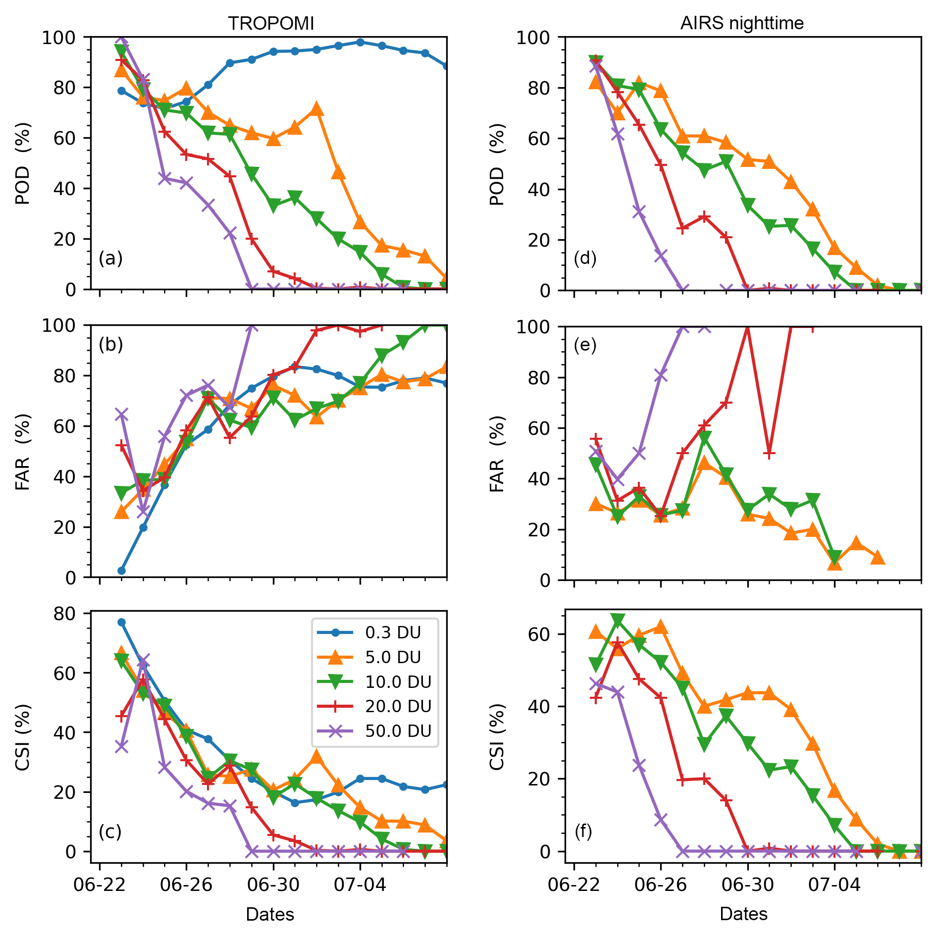
Figure 13 Left panels (a–c): time series of the probability of detection (POD; a), false alarm rate (FAR; b), and critical success index (CSI; c) for a forward simulation initialized by the reconstructed injection parameter based on TROPOMI data. The TROPOMI retrievals are used as reference observations. Subplots in the right panels (d–f) are the same as the left panels but for AIRS nighttime data, and the reference observations are also from the AIRS nighttime data. Color coding indicates the column density threshold used to detect events (see plot key).

When increasing the detection threshold, however, the model performance decreases. For instance, the POD shows a clear decreasing trend when the detection threshold is increased from 0.3 to 50 DU (Fig. 13a). The differences of the FAR between the different detection thresholds are smaller (Fig. 13b). This result suggests that although the forward simulation reproduced the overall spatial extent of the SO₂ clouds well, it has less ability to reproduce the internal structure and the location of the maxima of the SO₂ clouds. For example, the POD at all SO₂ thresholds except for the 0.3 DU level decreased notably during the first week of July (Fig. 13a), agreeing with our earlier findings that the forward simulation has lost the ability to capture structures of the SO₂ clouds at this time.

For comparison, we also assessed the performance of the forward simulation initialized by the AIRS nighttime SO₂ product with reference to the AIRS nighttime SO₂ product (Fig. 13d–f). As the AIRS retrievals have a higher background level (about 5 DU), the lowest detection threshold of 0.3 DU to assess the CSI is not very meaningful in this case. The trend and magnitude of the POD from AIRS retrievals are very similar to the simulation with TROPOMI retrievals, but the FAR has lower values of 20 %–40 %. During the first 10 d of the simulation, the CSI values for a detection threshold of 5.0 DU are between 40–80 %, which is about 1.5 times higher than for the simulation with TROPOMI retrievals.

To make a comparison between forward simulations with different initializations, we used the TROPOMI retrievals as a common reference, and the detection threshold was set to 5.0 DU. Figure 14 shows the POD, FAR, and CSI time series of forward simulations initialized with the TROPOMI SO₂ product, the AIRS nighttime SO₂ product, a constant injection rate, and the VolRes profile. The POD, FAR, and CSI are very consistent between forward simulations initialized with TROPOMI and AIRS nighttime retrievals. Compared with the simulation with a constant injection rate, the POD is constantly higher for simulations initialized by satellite retrievals. However, the simulations initialized with the satellite retrievals suffer from higher FAR between 29 June and 4 July. The simulation using the VolRes profile yields a similar POD level and trend to the simulation initialized by a constant injection rate. In summary, the overall trends of POD, FAR, and CSI are generally similar between forward simulations with different initialization settings. This result indicates that the quality of the forward simulations is less affected by the injection parameters as estimated by the backward trajectory method, probably due to the fact that the major SO₂ injection occurred during a small time window at the beginning of the eruption in this case.

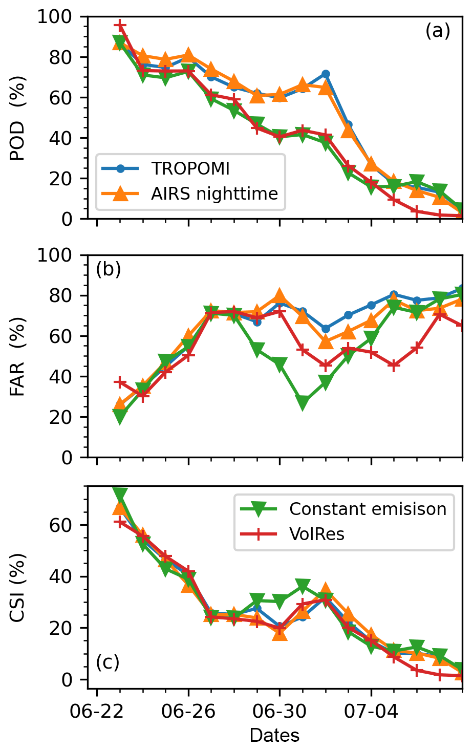
Figure 14 Time series of POD (a), FAR (b), and CSI (c) for forward simulations initialized by a constant injection rate (green) and the VolRes profile (red), as well as injection parameters reconstructed using TROPOMI (blue) and AIRS nighttime data (orange), respectively. The reference observations are TROPOMI retrievals. The column density threshold used to detect events is 5.0 DU.

3.2.4 Simulation of compact SO₂ clouds from late July to early August

From early July, the injected SO₂ from the Raikoke eruption has gradually faded away, and two compact SO₂ clouds became the major parts of the remaining SO₂. Figure 15 shows the location and distribution of the SO₂ clouds from 8 July to 9 August. During this period, the SO₂ is mainly concentrated in two compact clouds with a size of the magnitude of several hundred kilometers. On 8 July, the two compact SO₂ clouds are located close to each other, but eventually one of them moved toward the Asian continent (AC), and the other one moved toward North America (NA). In the following we refer to the SO₂ cloud that moved toward the Asian continent as the AC SO₂ cloud and the one toward North America as the NA SO₂ cloud.

Figure 15 Composite maps of the compact SO₂ clouds moving toward the Asian continent (a) and North America (b), respectively. The time of observation for each patch is indicated as text in the form of MMDDHH (month–day–hour) of the year 2019.

The AC SO₂ cloud first moved westward toward the Raikoke volcano and moved over the volcano on 15 July. After that, the AC SO₂ cloud moved eastward, and from 24 July it moved southwestward. After it reached 30^∘ N on 29 July, it stayed at this latitude and moved westward. During the whole period between late July and early August, the AC SO₂ cloud remained confined in a compact structure. The AC SO₂ cloud with a confined structure remains detectable in satellite retrievals until late August and September 2019 (Chouza et al., 2020; Gorkavyi et al., 2021).

The unique structure of the AC SO₂ cloud motivated us to test the ability of the Lagrangian model in simulating the transport and dispersion of the SO₂ cloud, especially the parameterization of the dispersion processes. In each orbit where TROPOMI detected the AC SO₂ cloud, the SO₂ detections were resampled to a number of 10 000 air parcels with equal mass to represent the SO₂ cloud. The number of air parcels was scaled proportional to the SO₂ vertical column density. The altitude for all the satellite retrievals is set to the altitude retrieved by the Cloud-Aerosol Lidar with Orthogonal Polarization (CALIOP) instrument (Gorkavyi et al., 2021). Note that CALIOP measures aerosol particles, which may introduce uncertainties regarding the altitude of gas phase SO₂. To reduce uncertainties associated with the vertical spread of the SO₂ in the simulations, the altitude of the air parcels corresponding to the same TROPOMI orbit was set to a constant value; i.e., the SO₂ was restricted to occur at the same altitude, and no vertical spread was introduced during resampling. During 17 to 21 July 2019, the aerosol altitude is ∼18 km, and it rises to ∼20 km during 24–27 July, after which it gradually rises to 24 km around 14 August 2019 (Gorkavyi et al., 2021). We used the resampled air parcels for TROPOMI retrievals during 17 July 2019 (Fig. 15) to initialize the forward simulation. Medians of the locations (longitudes and latitudes) of the air parcels are used to represent the location of the SO₂ cloud. The median absolute deviation (MAD) is used to measure the degree of dispersion of the SO₂ cloud.

Qualitatively, we compared the simulated AC SO₂ cloud with satellite retrievals at 1, 3, and 5 d after the initial release of the air parcels (Fig. 16). Dispersion in the simulations is in default settings, but different vertical motion schemes driven by vertical velocity (kinematic) and potential temperature (isentropic) are compared. As already shown in Fig. 15, the spatial extent of the AC SO₂ cloud is restricted in a limited bubble-like area during these times. One day after the start of the forward simulations, the model still captures the spatial distribution of the AC SO₂ cloud well (Fig. 16a and b). Despite the mean location being still captured by the model, the simulated SO₂ cloud is already too dispersive after 3 d. Although dispersion in both simulations is too strong, the simulation with constant isentropic vertical motions shows relatively weaker dispersion. In addition to dispersion, the simulated SO₂ cloud also shows some stretching effects along the west–southwest and east–northeast direction (Fig. 16g and h). Besides the horizontal location, however, both simulations driven by vertical velocity and constant potential temperature cannot correctly simulate the rising rate or the altitude of the SO₂ cloud (not shown). Although manual corrections to the altitude position of the SO₂ cloud have been performed in a previous study (Gorkavyi et al., 2021), in our study the vertical motion is freely driven by vertical velocity or remained confined to a constant potential temperature level.

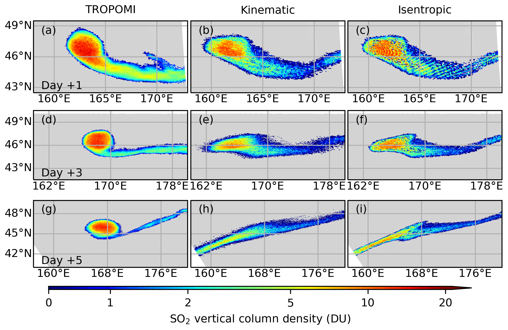
Figure 16 Forward simulation of the dispersion of the AC SO₂ cloud. Top row (a–c): spatial distribution of SO₂ vertical column density from TROPOMI at 18 July 2019, 02:33 UTC (a), and the corresponding distribution in forward simulations, in which vertical motion was driven by vertical velocity (b) or by constant potential temperature (c), respectively. Middle and bottom rows are the same as the top row but for 20 July 2019, 01:55 UTC, and 22 July 2019, 01:18 UTC, respectively.

The simulation of the dispersion of the AC SO₂ cloud was further evaluated by analyzing the MAD in longitude and latitude. Evaluation of the dispersion in the vertical direction is not available as the vertical spread of SO₂ is not fully observed. We designed separate experiments to test the role of subgrid-scale variance and the role of diffusivity. When testing the subgrid-scale variance, the diffusivities were set to zero and vice versa when testing the subgrid-scale variance. Figure 17 shows the mean trajectories and the degree of dispersion of the AC SO₂ cloud in satellite retrievals and forward simulations using different parameterizations of the subgrid-scale variance (the parameterizations on the horizontal and vertical directions are changed simultaneously). In general, all the forward simulations reproduce the trajectory of the retrieved AC SO₂ cloud (Fig. 17a). The MAD of the AC SO₂ in the TROPOMI SO₂ product is ∼1^∘ in the longitude dimension and ∼0.6^∘ in the latitude dimension. A common problem in the simulations is that the simulated dispersion is much stronger than the dispersion in satellite observations, even when the dispersion parameters were set to zero, and just the initial horizontal spread of the cloud was taken into account. In the longitude dimension, the MAD in simulations is roughly 1 order of magnitude larger than the MAD in the TROPOMI data after 5 d of simulation time. In contrast, in the latitude dimension, the MAD in the simulation is similar to the MAD in the TROPOMI data during the first ∼10 d of the simulation. After 10 d the MAD increased substantially in the simulations but not in the TROPOMI data. Still, the differences of the MAD in latitude between satellite retrievals and simulations are much smaller than the MAD differences in longitude. This result again suggests a stretching effect due to horizontal wind shear along the longitude direction beside the stochastic effects of dispersion.

Figure 17 Trajectories (a) and degree of dispersion (b) in the longitude dimension and (c) in the latitude dimension of the AC SO₂ cloud in simulations driven by vertical velocity but with different subgrid-scale diffusion settings (see color bar). Results from TROPOMI data are shown in black. Results from the simulations (diffusion module is set to default in both simulations) with vertical motion driven by vertical velocity and potential temperature are shown in red and magenta, respectively.

We also tested the role of diffusivity ranging from 10⁻² to 10³ times of the default diffusivity values (see Sect. 2.3 for reference). Similar to the results in Fig. 17, the simulated dispersion is too strong, but the simulation is more sensitive to diffusivity than subgrid-scale variance (Fig. 18). When the diffusivity is on the order of ≥10 times of the default diffusivity values, the simulation also does not capture the trajectory of the AC SO₂ cloud anymore.

Figure 18 Same as Fig. 17 but for simulations driven by different diffusivity settings (see color bar).

We performed forward trajectory simulations with vertical motion driven by constant potential temperature to avoid potential vertical velocity fluctuations due to data assimilation. The degree of dispersion shows less sensitivity to the dispersion parameters, and simulated MAD values for longitude and latitude are very close to the results from the default setting (Fig. 17). As the vertical position is adjusted at every time step to retain a constant potential temperature, the dispersion in the vertical direction is suppressed in the isentropic mode. Further, as the AC SO₂ cloud is located in the stratosphere, the turbulent diffusion is driven by vertical diffusivity, which is also switched off in the isentropic mode. Therefore, dispersion in the isentropic trajectory simulation is less sensitive to the choice of dispersion parameters and is weaker than the dispersion in kinematic mode. Taken together, our tests on the dispersion parameters suggest that the reason why the simulated SO₂ cloud generally is too dispersive is not only due to too strong diffusion in the model, but the stretching effect associated with horizontal wind shear also seems to play an important role.

4 Discussion

The injection parameters of a volcanic eruption, i.e., the time, altitude, and rate of SO₂ injections, have fundamental impacts on transport and dispersion simulations of volcanic ash and trace gases. Our study used two independent SO₂ satellite data products (from AIRS and TROPOMI, respectively) and a backward trajectory method implemented with the MPTRAC Lagrangian transport model to estimate the injection parameters of the 2019 Raikoke eruption. The reconstructed injection parameters generally agree with each other when different satellite datasets and meteorological reanalyses were used, indicating the robustness of our approach.

Our reconstruction shows that the SO₂ from the Raikoke eruption was mainly injected between 4 and 16 km of altitude, which falls within the range of previous studies (Hedelt et al., 2019; Muser et al., 2020; de Leeuw et al., 2021; Horváth et al., 2021). Similar to de Leeuw et al. (2021), our reconstruction also shows enhanced SO₂ concentrations at 12–14 km of altitude. Besides the overall agreement with the injection parameters used in this previous study, our reconstruction differs in some aspects. First, we estimated a total SO₂ injection of 2.1 ± 0.2 Tg, which is larger than earlier estimates of 1.5 ± 0.2 Tg (Global Volcanism Program, 2019; Muser et al., 2020; de Leeuw et al., 2021). Compared with the VolRes team estimation, de Leeuw et al. (2021) also argued that 1.5 Tg would underestimate the SO₂ mass in their forward simulation with the NAME model, and they suggested that either more SO₂ should be injected into the stratosphere (1.09 Tg), or a total of 2.0 Tg would be needed to match the TROPOMI retrievals on timescales >1 week. The stratospheric injection in our reconstruction is 0.85 ± 0.08 Tg, which is lower than the mass used by de Leeuw et al. (2021) but is significantly larger than the 0.64 Tg injection into the stratosphere in the VolRes profile.

Secondly, our reconstruction shows continuous but weak SO₂ injections after the first major injection on 21–22 June 2019. The major eruption during 21–22 June injects 1.5–1.6 Tg of SO₂, and a remaining fraction of 0.5–0.6 Tg of SO₂ was injected during 23–30 June, mainly into the troposphere. Hedelt et al. (2019) also suggested minor injections on and after 23 June. A direct validation of injections after 22 June is difficult, as the injection rates are rather low. We inspected Vis and IR images from Himawari 8 (not shown) and found that some volcanic plumes are visible over the Raikoke during 24–25 June, corresponding to the second plume in our reconstruction. However, due to high-altitude clouds, it is hard to validate or rule out the possibility of a third plume. From our forward simulations, the second and third plume are potentially overestimated. In the current setting, the backward trajectory method would only pick the first hit to identify a new source, and the second overpass will be not counted anymore. In reality, however, the SO₂ may have passed the volcano multiple times, which may lead to an overestimation for the second and the third plume. However, totally excluding either of these injections would cause other problems in the simulations, in particular in simulating the SO₂ total mass. A future study, based on more sophisticated inverse modeling techniques (Heng et al., 2016), might yield an improved injection reconstruction.

Forward simulations using our reconstructed injection parameters compare well with the TROPOMI SO₂ retrievals during the first 10 d after the eruption in terms of location and spatial extent. Similar to the simulation using NAME (de Leeuw et al., 2021), our simulation also shows limited skills in capturing the structures inside the SO₂ clouds at a later stage. de Leeuw et al. (2021) argued that the limited ability to capture the internal structure of the SO₂ clouds is because the diffusion in the model is too strong. Hence, we explored the influence of the diffusion parameterization on the simulation of the compact SO₂ cloud from late July to early August, as in Gorkavyi et al. (2021). Although the simulation skill was improved when reducing the strength of the simulated diffusion, the simulation was still too diffusive. As the simulations were still too diffusive when diffusion was switched off or when isentropic vertical motion was enforced to avoid jumps in the vertical velocity due to data assimilation (Stohl et al., 2005), we conclude that the strong dispersion is due to the meteorological input data itself. In particular, the stretching of the simulated SO₂ cloud (Fig. 16) and much stronger dispersion in the longitude direction (Figs. 17 and 18) suggest that the spread of the simulated SO₂ cloud is likely caused by horizontal wind shear in the ERA5 data. We did a similar set of experiments using ERA-Interim data, leading to the same results and conclusions.

Besides the above limitations, the current reconstruction and in turn the forward simulations may also be influenced by the selection of the TROPOMI products, i.e. the altitude of assumed SO₂ layer during retrieval, and by the lofting of the plume due to the co-existence of ash. TROPOMI SO₂ products are available for different scenarios that assume the SO₂ is at either 1, 7, or 15 km above sea level. The main difference between different products is the absolute value of the vertical column density, and it has a minor influence on the reconstruction of the relative injection rate. However, the different SO₂ can result in a different mass estimate. Comparison of the total SO₂ mass between the 7 and 15 km retrieval products for TROPOMI shows that the mass is identical during the first week of the eruption. After the first week, the mass derived from the 7 km product is consistently higher than the 15 km product by ∼10 %. Therefore, using the 7 km product would get an higher estimate of the total SO₂ mass, which is at the upper limit of the estimate reported in this study. On the other hand, Muser et al. (2020) reported a lofting effect of ash for the Raikoke plume during the initial days after the eruption. The lofting effect may also exist during the period of the compact SO₂ (Gorkavyi et al., 2021). Such a lofting effect would directly influence the forward simulation as it is not reflected in the meteorological data (Sect. 3.2.4) and may need manual tuning to correctly simulate the long-range transport of the SO₂. As the vertical column density was used in the reconstruction, and it does not contain vertical information, the lofting effect may have less influence on the reconstruction. A quantitative assessment of the impact of the lofting effect is however unavailable from the current study, and it should be considered in a future study.

Our study estimated the overall SO₂ e-folding lifetime during the first 3 weeks after the Raikoke eruption to be 13–17 d. This finding was consistent between using a simple exponential decay of the reconstructed SO₂ injections and simulating chemical loss of SO₂ due to reaction with hydroxyl. The SO₂ mass burden, derived from both the exponential decay experiment and the hydroxyl module of MPTRAC, matches well with the TROPOMI retrievals. Our estimation also agrees with earlier studies. de Leeuw et al. (2021) estimated that the e-folding lifetime after 27 June is 14–15 d. Based on Ozone Mapping and Profiler Suite (OMPS) retrievals, Gorkavyi et al. (2021) estimated that the e-folding lifetime during the first 20 d after the eruption is 18.9 d, which is slightly larger than the e-folding lifetime in our study and in de Leeuw et al. (2021). We note that, however, the e-folding lifetime has a strong dependence on the altitude of the SO₂ layer (Fig. 10), emphasizing that correctly determining the vertical profile of the injection rates is essential to reproduce the retrieved SO₂ mass change.

5 Conclusions

Determining the injection parameters of volcanic eruptions, including the plume altitude, time, and injection rate, is essential for accurately simulating the dispersion of volcanic trace gases and aerosols. We used the MPTRAC model as well as AIRS and TROPOMI satellite retrievals to estimate the injection parameters of the 2019 Raikoke eruption. The altitude and time of the SO₂ injection were estimated based on a backward trajectory method and the SO₂ retrievals from the AIRS and TROPOMI satellites. Then, we used an exponential decay model to calibrate total injected SO₂ mass with the SO₂ mass from TROPOMI retrievals. The lifetime of SO₂ was estimated to be 13–17 d. Our estimation of the SO₂ mass change in the exponential experiments agrees well with the mass change in the forward simulation that is driven by chemical reactions. Both methods reproduced the mass change derived from TROPOMI retrievals. Therefore, our method is robust for estimating the whole set of injection parameters, i.e., the time, altitude, and injection rate, for SO₂ injections.

Our estimated total SO₂ mass for the 2019 Raikoke eruption is 2.1 ± 0.2 Tg, which is larger than the initial estimate of 1.5 ± 0.2 Tg from earlier studies; 40.5 % (0.85 Tg) of the total SO₂ mass was injected into the lower stratosphere. We consider our new estimation of a larger amount of SO₂ reasonable, as it better reproduces the satellite-retrieved mass change in the forward simulations than assuming an injection of 1.5 Tg SO₂ either by a constant injection rate or following the VolRes profile (Fig. 9). The reconstructions of injection parameters are very consistent between using the TROPOMI daytime and AIRS nighttime products. Forward simulations driven by our reconstructed time- and height-resolved injection parameters compared with simulations driven by a simple constant injection rate, an approach that is common in global chemistry climate simulations, show better performance of reproducing the satellite retrievals, especially in terms of spatial extent and location. The findings from this study will help us to create a long-term volcanic SO₂ injection inventory from AIRS, which we hope might be useful to improve chemistry climate simulations considering the effects of volcanic SO₂ in future work.