Atmospheric gas-phase composition over the Indian Ocean

The Indian Ocean is coupled to atmospheric dynamics and chemical composition via several unique mechanisms, such as the seasonally varying monsoon circulation. During the winter monsoon season, high pollution levels are regularly observed over the entire northern Indian Ocean, while during the summer monsoon, clean air dominates the atmospheric composition, leading to distinct chemical regimes. The changing atmospheric composition over the Indian Ocean can interact with oceanic biogeochemical cycles and impact marine ecosystems, resulting in potential climate feedbacks.

Here, we review current progress in detecting and understanding atmospheric gas-phase composition over the Indian Ocean and its local and global impacts. The review considers results from recent Indian Ocean ship campaigns, satellite measurements, station data, and information on continental and oceanic trace gas emissions. The distribution of all major pollutants and greenhouse gases shows pronounced differences between the landmass source regions and the Indian Ocean, with strong gradients over the coastal areas. Surface pollution and ozone are highest during the winter monsoon over the Bay of Bengal and the Arabian Sea coastal waters due to air mass advection from the Indo-Gangetic Plain and continental outflow from Southeast Asia. We observe, however, that unusual types of wind patterns can lead to pronounced deviations of the typical trace gas distributions. For example, the ozone distribution maxima shift to different regions under wind scenarios that differ from the regular seasonal transport patterns. The distribution of greenhouse gases over the Indian Ocean shows many similarities when compared to the pollution fields, but also some differences of the latitudinal and seasonal variations resulting from their long lifetimes and biogenic sources. Mixing ratios of greenhouse gases such as methane show positive trends over the Indian Ocean, but long-term changes in pollution and ozone due to changing emissions and transport patterns require further investigation. Although we know that changing atmospheric composition and perturbations within the Indian Ocean affect each other, the impacts of atmospheric pollution on oceanic biogeochemistry and trace gas cycling are severely understudied. We highlight potential mechanisms, future research topics, and observational requirements that need to be explored in order to fully understand such interactions and feedbacks in the Indian Ocean region.

1 Introduction

Over the Indian Ocean, intense anthropogenic pollution from Southeast Asia mixes with pristine oceanic air. The interplay of the polluted continental and clean oceanic air masses as well as the resulting atmospheric composition, are determined by distinct seasonal circulation patterns. The large-scale monsoon circulations, in combination with anthropogenic emissions from southern Asia, lead to seasonally contrasting chemical regimes over the Indian Ocean. As the anthropogenic emissions include relatively large contributions from biofuel–biomass combustion and incomplete industrial burning, the atmospheric composition during polluted periods shows unique characteristics when compared to other regimes. The complex mixture of chemical constituents and large-scale transport patterns can have a profound influence on oceanic processes, stratospheric composition, and neighboring regions such as the Mediterranean and Africa. Here we provide a review of the recent progress in our understanding of the atmospheric gas-phase composition over the Indian Ocean and how it impacts the ocean and upper atmosphere. This article is part of the special issue “Understanding the Indian Ocean system: past, present and future”.

1.1 Region

The Indian Ocean is the world's third-largest ocean, covering 19.8 % of the water on the Earth's surface. In contrast to the Pacific and Atlantic oceans, it does not stretch from pole to pole but is enclosed on three sides by major landmasses and an archipelago. The Indian Ocean is centered on the Indian Peninsula, which also forms the northern border together with Iran, Pakistan, and Bangladesh. In the west, the Indian Ocean is bounded by East Africa and the Arabian Peninsula, while the eastern and southern boundaries are set by Southeast Asia, Australia, and the Southern Ocean.

The countries bordering the Indian Ocean are home to one-third of the world's population, accounting for approximately 2.5 billion people (Roser et al., 2013). The economies of many Indian Ocean countries are expanding rapidly, with India being the fastest growing major economy in the world. Similarly, many Indian Ocean countries show rapid population growth, which is expected to further increase in the future. Given the quickly growing populations and industries, the Indian Ocean is becoming a pivotal zone of strategic political competition. At the same time, the Indian Ocean hosts a large variety of marine ecosystems including coral reefs, seagrass beds, and mangrove forests. Anthropogenic activities along the coastlines and climate change threaten biodiversity in the Indian Ocean, which contains 25 % of the Earth's biodiversity hotspots (Mittermeier et al., 2011).

Growing populations also lead to rapidly increasing anthropogenic emissions. Burning conditions are often poorly controlled, for instance during biofuel burning in cookstoves and fossil fuel burning in vehicles (Li et al., 2017). Together with burning of coal and other fossil fuels for energy production, this leads to large emissions of manmade trace species including greenhouse gases and ozone precursors (e.g., Lawrence, 2004). In addition, primary aerosols, such as soot and dust, and precursors of secondary aerosols are released in relatively large amounts. As a result, air pollution is a serious health issue in many Indian Ocean countries, leading to increases in respiratory and cardiovascular problems (Rajak and Chattopadhyay, 2020). The intense pollution has also been linked to regional weather impacts, such as changes in rainfall patterns and decreasing crop harvests (e.g., Bollasina et al., 2011; Li et al., 2016).

1.2 Seasons

Seasonal changes in atmospheric transport patterns are the main driver of Indian Ocean chemical regimes and lead to periods of intense anthropogenic pollution alternating with periods of clean oceanic air. The South Asian monsoon circulation, the strongest monsoon system in the world, dominates the regional meteorology of the Indian subcontinent. The seasonal reversal of the winds is coupled to a strong annual cycle of precipitation with very wet summer and dry winter conditions (Chang, 1967). Being the dominant driver of the annual cycle of rainfall, the South Asian monsoon controls the water and food security of the region and thus the well-being and prosperity of large populations.

The monsoon system also has a strong impact on the atmospheric composition over the Indian Ocean. During the winter monsoon from December to February, continental aerosols as well as man-made trace species and their reaction products dominate the chemical regime (Lelieveld et al., 2001). A layer of air pollution is visible on satellite pictures as a brown haze hanging over much of South Asia and the Indian Ocean. This so-called Indian Ocean brown cloud has been suggested to impact regional climate by masking greenhouse-gas-induced surface warming (Ramanathan et al., 2005) and to affect monsoon rainfall.

In contrast, clean air dominates the atmospheric composition over the Indian Ocean during the summer monsoon from June to September, leading to a completely different chemical regime. Atmospheric pollutant levels over the Indian Ocean are low, and typical open-ocean background conditions can be observed (Lawrence and Lelieveld, 2010). While boreal summer conditions prevent the anthropogenic pollution from spreading across the Indian Ocean, an anticyclonic circulation, centered at 200 to 100 hPa, offers an efficient pathway for continental pollution into the global upper troposphere and lower stratosphere (UTLS) (e.g., Randel et al., 2010; Lelieveld et al., 2018).

Finally, during the monsoon transition periods from April to May and September to October, the offshore pollution is less strong due to weaker air mass transport from Southeast Asia and Africa over the Indian Ocean (Sahu et al., 2006).

1.3 Early work

The largest international scientific study exploring the impact of South Asian emissions on the composition of the atmosphere over the Indian Ocean, the Indian Ocean Experiment (INDOEX), took place during the winter monsoon in 1999, with some pilot campaigns conducted during 1996–1997. During the multi-platform field campaign, surprisingly high pollution was detected over the entire northern Indian Ocean all the way to the Intertropical Convergence Zone (ITCZ). Scientific studies revealed that the nature of the pollution was considerably different from that in Europe or North America, with strongly enhanced carbon monoxide concentrations related to widespread biofuel use and agricultural burning (e.g., Lelieveld et al., 2001). Other large pollution sources based on fossil fuel combustion and biomass burning were linked to high loads of sunlight-absorbing aerosols with potential consequences for the regional atmospheric energy balance (Ramanathan et al., 2002). A few years before INDOEX, the Joint Global Ocean Flux Study (JGOFS) India investigated the factors controlling carbon fluxes in the Arabian Sea and led to estimates of CO₂ emissions to the atmosphere for this region (Sarma et al., 2003).

The INDOEX findings, presented in many scientific publications, drew attention to this region and several projects and campaigns followed over the next decade. The Bay of Bengal Experiment (BOBEX) research cruise during February to March 2001 detected high ozone and pollution levels over the Bay of Bengal and linked them to transport from the continent (Naja et al., 2004; Lal et al., 2006). The southern Indian Ocean was explored during the Pilot Expedition to the Southern Ocean (PESO) research cruise from January to April 2004, which revealed much cleaner air masses with smaller aerosol loadings in the region south of the ITCZ (Pant et al., 2009). Other research cruises, such as the Bay of Bengal Processes Studies (BOBPS) during September to October 2002, investigated oceanic productivity and nutrients in relation to air–sea exchange of climate-active gases (Sardessai et al., 2007). A detailed overview of research cruises, island measurements, and aircraft campaigns investigating the atmosphere over the Indian Ocean is given in Lawrence and Lelieveld (2010). The authors provide a comprehensive review of the state of the art at this time by bringing together observational and modeling studies.

1.4 Scope and organization of this study

Here we will focus on recent progress in the field by giving an overview of results published after 2010. We will synthesize the current understanding of Indian Ocean gas-phase atmospheric composition and explore how it is driven by emission sources, transport, and chemistry. Our region of interest encloses the Indian Ocean from 30^∘ S to its northern continental borders and across its whole longitudinal range. It also includes neighboring landmass such as parts of East Africa, the Arabian Peninsula, South Asia, Southeast Asia, and Australia as depicted in Fig. 1. This review focuses on three groups of atmospheric gases: (1) ozone and pollutants – carbon monoxide (CO), nitrogen oxides (NO_x), sulfur dioxide (SO₂), ammonia (NH₃), and mercury; (2) greenhouse gases – methane (CH₄), nitrous oxide (N₂O), carbon dioxide (CO₂), and carbonyl sulfide (COS); and (3) volatile organic compounds (VOCs) and short-lived biogenic gases – dimethylsulfide (DMS), isoprene, and halogen compounds.

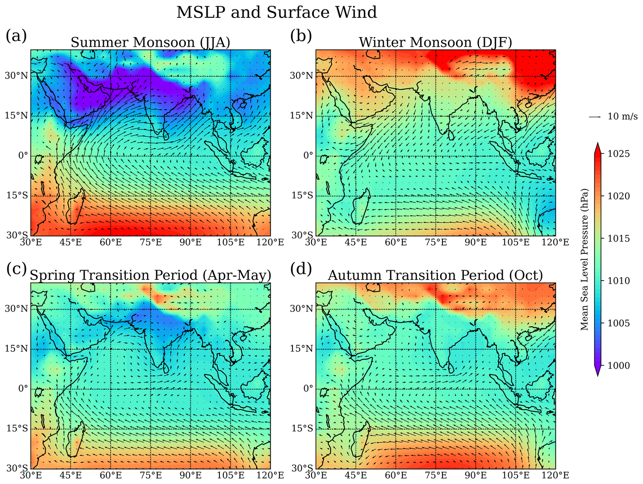
Figure 1 Mean surface-level pressure (MSLP) and surface wind for (a) summer monsoon 2018 (June–August), (b) winter monsoon 2018–2019 (December–February), (c) spring transition 2018 (April–May), and (d) autumn transition 2018 (October) from ERA-Interim.

Section 2 provides an overview of the physical processes in the atmosphere and ocean that are relevant for the atmospheric composition. Section 3 will introduce all campaigns and measurements that are the basis for scientific studies published after 2010 and discussed here. Regional sources and sinks of greenhouse gases, pollution, and biogenic trace gases will be given in Sect. 4. Short introductions to all gases listed above, including their role in the atmosphere, can also be found in Sect. 4. The focus of Sect. 5 is on our current knowledge of the atmospheric composition over the Indian Ocean and how it is driven by physical processes and regional sources. We will present a synthesis of the scientific progress made after 2010 in Sect. 6, where we will also discuss the global and local impacts of the Indian Ocean atmospheric composition. An outlook and a summary of current knowledge gaps are given in Sect. 7. A key for all abbreviations used in this paper is provided in Appendix A.

2 Physical processes

2.1 Atmospheric processes

The South Asian monsoon circulation dominates the transport patterns and regional meteorology over the Indian Ocean. Strong seasonal circulation changes give rise to three main meteorological regimes: the summer monsoon from June to September, the winter monsoon from November to March, and the transition periods from April to May and from the end of September to October. Surface flow patterns as well as seasonal transport regimes are described in the following subsections, while a discussion of intraseasonal and interannual variability can be found in Sect. S1 in the Supplement.

2.1.1 Near-surface flow patterns

A detailed picture of the near-surface flow patterns is provided in Fig. 1 in the form of seasonal mean surface wind fields and sea level pressure derived from 2018–2019 ERA-Interim reanalysis data. Seasonal mean plots here and in the rest of the paper are shown for core monsoon and transition periods, i.e., June to August (JJA) for the summer monsoon, December to February (DJF) for the winter monsoon, April to May (April–May) for the boreal spring transition period, and October (October) for the boreal autumn transition period. The equatorial and northern Indian Ocean (north of 10^∘ S) is dominated by seasonally reversing monsoon winds (Schott and McCreary, 2001; Schott et al., 2009). Southwest winds occur during the summer monsoon with the low-pressure system of the ITCZ shifted north of 15^∘ N (Fig. 1a), while northeast winds occur during the winter monsoon with the low-pressure belt situated south of the Equator (Fig. 1b). Over the southern Indian Ocean (south of 10^∘ S), steady southeast trades prevail during all seasons but reach further northward during the northern summer.

The seasonally reversing monsoon winds and inter-hemispheric pressure gradients over the equatorial Indian Ocean are a striking feature different from the other tropical oceans, where sustained easterly winds are found along the Equator. In contrast, equatorial winds over the Indian Ocean are westerlies during the monsoon transition periods (Fig. 1c and d) and show a weak westerly annual mean component (Lamb and Hastenrath, 1979). These equatorial westerlies are driven by an interplay of an eastward pressure gradient along the Equator, the latitudinal position of the flow recurvature, and the strength of the trade winds (Hastenrath and Polzin, 2004).

2.1.2 Summer and winter monsoon

During the summer monsoon, steady onshore winds transport air from the ocean over to the continent, where it results in deep convection and the well-known Indian summer monsoon rains. Air masses experiencing fast upward transport in convective updrafts converge in the upper troposphere, forming a high-pressure system. The associated anticyclone circulation is tied to the outflow of the deep convection and is situated directly over highly polluted southern Asia. As a result, distinct tracer anomalies have been observed in the anticyclone, indicating strong upward transport of pollution from the surface (e.g., Randel et al., 2010). Given the dynamical confinement of tropospheric tracers and aerosols in the anticyclone, the Asian monsoon system provides a potentially efficient pathway from the surface to the tropical UTLS. However, a significant fraction of the pollution can be removed from the air mass before entering the stratosphere due to lightning-driven OH reactions in monsoonal convection (Lelieveld et al., 2018).

During the winter monsoon, the prevailing northeasterly winds reverse the meteorological situation. There is little rain over southern Asia, marking this as the “dry season”, and the missing convection chemically disconnects the surface layer from the upper troposphere (Kunhikrishnan et al., 2004). Instead, pollution outflow occurs in the marine boundary layer (MBL) via offshore winds towards the northern Indian Ocean down to the Equator. Primary MBL flow channels have been identified in the western Arabian Sea, the eastern Arabian Sea just off the Indian west coast, the western Bay of Bengal, and Southeast Asia (Krishnamurti et al., 1997a, b; Verver et al., 2001).

Winter monsoon flow patterns are further complicated by effects of the land–sea breeze, which lofts coastal air masses above the MBL (Simpson and Raman, 2004). The associated offshore flow above the MBL transports air masses over the coastal oceans, where they constitute the so-called “elevated layer”. Due to the relatively rapid outflow, the elevated layer provides an additional effective mechanism for pollution transport from the continents towards the Indian Ocean (Lawrence and Lelieveld, 2010). As a result, outflow during the winter monsoon occurs in two distinct layers, namely the pollutant plume within the MBL (up to 800–1000 m) and the elevated layer (1–3 km). Once over the northern Indian Ocean, the northeasterly trade winds transport the air masses towards the ITCZ, typical within 7–10 d (Ethé et al., 2002). Similarly, over the southern Indian Ocean, southeasterly winds transport pristine boundary layer air masses northwards. At the ITCZ, these trade wind flows converge, and associated convection transports the air upwards into the upper troposphere (Iyengar et al., 1999).

Over the western part of the tropical Indian Ocean, the ITCZ has been observed to occur simultaneously in two bands on either side of the Equator, forming the so-called double ITCZ (Meenu et al., 2007), throughout the year. Based on cloud characteristics and outgoing longwave radiation, the most preferred latitudes for the northern and southern bands of the ITZC were found to be around 5^∘ N and 7.5 to 10^∘ S.

2.2 Oceanic processes

The physical oceanography of the northern Indian Ocean reflects the seasonal changes in the monsoon cycle, including impacts on currents, thermohaline circulation, sea surface temperature (SST), salinity, and upwelling events, while the equatorial and southern Indian Ocean does not experience this influence. For more details about general Indian Ocean physical processes, please see Schott et al. (2009) and references therein, Phillips et al. (2021) from this issue, and Sect. S2. In the following sections, we concentrate on how physical oceanography affects salinity, SST, and biological productivity, which in turn play a major role in controlling air–sea exchange and atmospheric composition, in particular for biogenic trace gases such as bromoform (CHBr₃), DMS, and isoprene

Salinity, SSTs, and productivity

On seasonal timescales, freshwater input due to rainfall and river discharge is important for the salinity balance in the Bay of Bengal, and horizontal advection related to the monsoon plays a dominant role in the northern Indian Ocean (Rao and Sivakumar, 2003; Da-Allada et al., 2015). In the southwestern tropical Indian Ocean, the freshwater flux due to precipitation is a major control on the salinity (Da-Allada et al., 2015). The rainfall over the Indian Ocean shows a general migration to the summer hemisphere following sunlight and warm SSTs, highlighting their strong coupling. Conversely, latent heat loss caused by cool, dry air from the Asian continent leads to strong wintertime cooling in the northern Arabian Sea. The strong summertime cooling in parts of the Arabian Sea instead is a combined result of latent heat loss caused by the strong southwesterly winds as well as upwelling and offshore advection from the Somali and Omani coasts. During boreal summer, upwelling-induced cooling off Somalia prevents atmospheric convection from the western Arabian Sea. From the eastern Arabian Sea to the South China Sea, north of the Equator, high SSTs promote atmospheric deep convection (Schott et al., 2009).

The oceanic upwelling caused by strong monsoonal winds supplies nutrients to the surface layer, where they support elevated rates of primary productivity. This occurs mainly in the Arabian Sea, the Somali Basin, along the Indian coast, and in the northern Bay of Bengal, especially during summer months. The seasonal reversals in the boundary currents of the northern Indian Ocean, including the seasonal switching from upwelling to downwelling circulations, have important biogeochemical and ecological impacts that modify primary productivity, nutrient stoichiometry, oxygen concentrations, and phytoplankton species composition (Hood et al., 2017). In addition, transient upwelling due to seasonal variations of currents and mesoscale variability can give rise to episodically high levels of primary production throughout the Indian Ocean coastal waters.

2.3 Long-term changes

2.3.1 Indian Ocean warming

The Indian Ocean has warmed steadily over the past century, with an SST increase of 1 ^∘C during 1951–2015, which is markedly higher than the global average SST warming of 0.7 ^∘C over the same period (Du and Xie, 2008; Han et al., 2014; Krishnan et al., 2020). Overall, this Indian Ocean averaged warming rate is broadly consistent across observational products (Dong et al., 2014; Yao et al., 2016) and historical simulations from the Coupled Model Intercomparison Project – Phase 5 (CMIP5). It can be largely attributed to anthropogenic forcing rather than natural external forcing, such as volcanic and solar variations (e.g., Dong et al., 2014). It has been shown that the basin-wide warming due to increasing greenhouse gases is slowed down by the indirect effects of anthropogenic aerosol (Dong and Zhou, 2014). In addition to anthropogenic forcing, the sustained warming over the Indian Ocean warm pool region is caused by local ocean–atmosphere coupled mechanisms, with their relative roles being debated (e.g., Dong et al., 2014; Du and Xie, 2008). The importance of the Indian Ocean in the global ocean heat budget was not recognized until the hiatus period at the beginning of the 21st century, during which the abrupt increase in the upper Indian Ocean heat content served as a major sink of the excessive heat entering the Earth system (e.g., Nieves et al., 2015).

The Indian Ocean warming is not spatially homogeneous in models or observations. The western tropical Indian Ocean has been warming for more than a century at a rate faster than any other region of the tropical oceans and is the largest contributor to the overall trend in the global mean SST (Roxy et al., 2014). Positive SST anomalies in the western part of the Indian Ocean have increased markedly since 1950, while negative events have been reduced (Cai et al., 2009). The warming of the generally cool western Indian Ocean against the rest of the tropical warm pool region (Roxy et al., 2014, 2015) and corresponding changes in the zonal SST gradient (Saha et al., 2014) have both been proposed as plausible explanations for the observed decrease in Indian monsoon rainfall over the last 3 decades. In addition, they have the potential to alter the marine food webs in this biologically productive region.

The Indian Ocean warming is projected to further increase over the course of the 21st century in response to unabated greenhouse gas emissions. By the end of the 21st century, the strongest warming in the Arabian Sea and western equatorial Indian Ocean is consistently projected in CMIP models, which could yield more Arabian Sea cyclones and a further decrease in monsoonal rains (Gopika et al., 2020).

2.3.2 Summer monsoon and precipitation

There are large uncertainties related to the variability in the South Asian summer monsoon in a changing climate. Several studies have debated whether the monsoon is weakening or strengthening, as well as the mechanisms driving the changes (Roxy et al., 2015). According to a review by D. Singh et al. (2019), observational and modeling studies have determined that the potentially weakened monsoon is due to a combination of forcings, such as land use and irrigation changes, increased greenhouse gases, and anthropogenic aerosols. Roxy et al. (2015) provide compelling evidence that Indian Ocean warming potentially weakens the land–sea thermal contrast and dampens the summer monsoon Hadley circulation, leading to reduced rainfall over parts of South Asia.

The Indian Ocean is one of the greatest moisture sources, accounting for nearly one-third of the total net transport of water toward the continents (Bengtsson, 2010). Both remote and local SST anomalies can induce hydrological cycle changes over the Indian Ocean, affecting local and remote precipitation. Han et al. (2019) showed that the moisture sources (evaporation minus precipitation) in the tropical central-eastern and southwestern Indian Ocean experienced a significant increase during boreal summer between 1979 and 2016. In addition, there has been a significant reduction in the annual frequency of tropical cyclones and their associated rainfall over the northern Indian Ocean since the middle of the 20th century (Krishnan et al., 2020). In contrast, the frequency of very severe cyclonic storms during the autumn transition season has increased significantly during the last 2 decades. At the same time, an enhanced rainfall contribution has occurred due to a higher precipitation efficiency (K. Singh et al., 2016, 2019), possibly leading to a dry atmosphere. Further changes in the Indian summer monsoon rainfall are expected for the future, but current model projections give contradicting results (e.g., Roxy et al., 2015; Zou and Zhou, 2013).

Changes in surface wind are expected to be moderate for the first half of the 21st century, with a noticeable decline of wind speed over the tropical Indian Ocean due to reduced thermal land–sea contrasts. The southern extratropical region and Southern Ocean, on the other hand, are expected to show a significant strengthening of the wind fields by the end of the 21st century (Mohan and Bhaskaran, 2019). Ocean–atmosphere feedback that is not well represented and coarse model resolutions, however, are known to lead to large uncertainties in model estimates of wind speed changes (Annamalai et al., 2017; Mohan and Bhaskaran, 2019).

2.3.3 Salinity and productivity

Du et al. (2015) noted freshening in the southeastern tropical Indian Ocean starting in the mid-1990s. Idealized model experiments suggest that multidecadal changes in subsurface ocean salinity during 1950–2000 were due to isopycnal migration related to ocean surface warming (Lago et al., 2016). However, the enhanced precipitation in the Maritime Continent and the strengthening of the Indonesian Throughflow are thought to be the likely causes of the freshening trend in the southeastern Indian Ocean since the early 2000s (Llovel and Lee, 2015; Hu and Sprintall, 2017).

While Behrenfeld et al. (2006) indicate a reduction in net primary productivity over most of the tropics as a result of surface thermal stratification, they have suggested an increase in primary productivity for the western Indian Ocean from 1998 to 2004. Recent biogeochemical simulations of the Arabian Sea ecosystem suggest that an intensification of monsoon winds strongly increases ecosystem productivity, thereby amplifying the oxygen biological consumption and intensifying the oxygen minimum zone (OMZ) at depth (Lachkar et al., 2018). At the same time, the near-surface area will experience increased ventilation due to the predicted stronger winds. On the contrary, a review in this issue summarizes evidence indicating a significant, but small, reduction in primary production in the northern Indian Ocean (Löscher, 2021). An alarming decrease of up to 20 % in marine phytoplankton during the past 6 decades has been identified in the western Indian Ocean (Roxy et al., 2016) driven by enhanced ocean stratification and suppressed nutrient mixing from subsurface layers. Gregg and Rousseaux (2019) also conclude from the assimilation of ocean color satellite data (1998–2015) into an ocean biogeochemical model that the decline in global ocean primary productivity of 2.1 % per decade is mainly driven by the northern and equatorial Indian Ocean. Any changes to biological processes have the potential to alter trace gas cycling in the surface ocean.

3 Campaigns, station data, and satellite measurements

A few Indian Ocean coastal or island stations have been operated as part of long-term scientific measurement programs or operational air quality networks, providing limited area observations. In addition, intensive ship and aircraft campaigns have been conducted for detailed investigations of atmospheric processes during short episodes. These data can be complemented by satellite observations of tropospheric composition, which provide the large-scale picture for a number of substances, albeit often with limited vertical resolution and reduced accuracy for individual measurements. In this section, we will give an overview of campaigns, station data, and satellite measurements that have been applied to study the atmospheric composition over the Indian Ocean over the last decade.

3.1 Campaigns and station data

Chemical, physical, and biogeochemical processes occurring in and above the Indian Ocean have been explored during various field campaigns. Here, all campaigns that have contributed to the recent progress in the field and led to publications after 2010 are summarized in Table 1. It should be noted that the ICARB multi-platform field experiment consisted of three phases, with the first phase exploring composition in the spring transition season of 2006 (ICARB), a second phase taking place during the winter monsoon of 2008–2009 (referred to as W_ICARB) supplemented by aircraft measurements, and a third phase during the winter monsoon of 2018 (referred to as ICARB-218).

Table 1 Summary of campaigns in the Indian Ocean for the 21st century.

In addition to dedicated campaigns, some island and coastal stations have conducted long-term measurements that provide valuable information about the atmospheric composition over the Indian Ocean.

CO₂ surface flask measurements from the Cape Rama site on the Indian coastline have been used to analyze the distribution and variability of CO₂ over this region for 2009–2012 (Nalini et al., 2018). Measurements of CH₄, another important greenhouse gas, and the pollutant CO are available from ground-based in situ cavity ring-down spectroscopy analyzers and Fourier transform infrared spectrometers at two sites on Reunion Island in the southern Indian Ocean (Zhou et al., 2018). These multi-annual time series (2011–2017) allowed investigating the impact of emissions from biomass burning in Africa and South America on atmospheric pollutant levels over the Indian Ocean. CO surface data are also available from the NOAA/ESRL Global Monitoring Division network station in Mahé (Wai et al., 2014).

In situ tropospheric ozone measurements were collected from 2003 to 2007 from balloon-borne electrochemical concentration cell sensors launched above Ahmedabad in western India (Lal et al., 2014). The continuous dataset enabled studies of the impact of transport processes on the seasonal cycle and on the vertical distribution of ozone. The observation site in Trivandrum situated on the southwest coast of India collected measurements of nitrogen oxides with a chemiluminescence NO_x analyzer from 2007 to 2009 (David and Nair, 2011).

3.2 Satellite measurements

Satellite measurements of atmospheric composition over the Indian Ocean have provided valuable information over the last decades that allowed for studies of the overall distribution and long-term changes in key substances. Most instruments used today apply passive remote sensing with observations being mainly done in nadir geometry. Here we will give a short overview of satellite instruments that provide measurements used in scientific studies of the Indian Ocean atmosphere. In addition, we have compiled plots of the seasonal CO, NO₂, and CH₄ surface distribution for this review article and will describe the respective satellite measurements in more detail.

3.2.1 Pollutants (NO₂) from OMI and TROPOMI

The Ozone Monitoring Instrument (OMI) is a key instrument on board NASA's Aura satellite. OMI is a nadir-viewing, wide-field-imaging spectrometer that measures backscattered radiances at a spectral resolution of 0.42–0.63 nm (Levelt et al., 2006). Its wide field of view of 114^∘ with a swath width of 2600 km yields daily global coverage with a spatial resolution of 13 km × 24 km (Liu et al., 2010). OMI measures ozone profiles as well as other key air quality components such as NO₂, SO₂, and aerosol characteristics. In this article, we use the OMI tropospheric NO₂ column product from 2003 to 2020 to analyze long-term changes over different coastal and open-ocean regions of the Indian Ocean (Sect. 6).

The TROPOspheric Monitoring Instrument (TROPOMI) is a nadir-viewing imaging spectrometer on board the Copernicus Sentinel-5 Precursor satellite, which was launched in October 2017 for a mission of 7 years. The satellite has a sun-synchronous orbit achieving nearly full surface coverage on a daily basis. TROPOMI contains four spectrometers, with three covering the ultraviolet and near-infrared wavelengths and one for the shortwave infrared range. Key atmospheric species observed by TROPOMI include ozone, NO₂, SO₂, CO, and aerosol properties. The TROPOMI tropospheric NO₂ column product (Boersma et al., 2018) shows improved spatial resolution compared to previous versions. The NO₂ retrieval algorithm is based on the NO₂ DOMINO retrieval previously used for OMI spectra with improvements made for all retrieval steps. In this article, we use the TROPOMI Level 2 NO₂ tropospheric column data product to show its distribution and seasonal variations (Sect. 5.1).

3.2.2 Pollutants (CO) from MOPITT

The Measurements of Pollution in the Troposphere (MOPITT) instrument is on board NASA's Earth Observing System Terra spacecraft, measuring tropospheric CO since March 2000. The satellite is in a sun-synchronous polar orbit of 705 km, allowing the instrument to make measurements in a 612 km cross-track scan with a footprint of 22 km × 22 km, providing global coverage every 3 d. The MOPITT measurements provide vertical profiles and total columns of CO, which are useful to analyze the distribution, transport, sources, and sinks on a global scale. CO retrieval products are generated with an iterative optimal-estimation-based retrieval algorithm based on the MOPITT calibrated radiances and a priori knowledge of CO variability. The recently released version 8 (V8) products benefit from updated spectroscopic information used in the radiative transfer model and improved methods for radiance bias corrections (Deeter et al., 2019). In this article, we use MOPITT V8 Level 3 monthly data (near and thermal infrared radiances) with day and night retrievals averaged to analyze the seasonal variation of the surface CO distribution (Sect. 5.1).

3.2.3 Greenhouse gases (CH₄ and CO₂) from GOSAT

The Greenhouse Gases Observing Satellite (GOSAT/Ibuki) is a sun-synchronous polar orbit satellite that measures CO₂ and CH₄ from the stratosphere to the Earth's surface. The retrieval precision for CO₂ is smaller than 3.5 ppm (Yoshida et al., 2011) utilizing the Thermal and Near-Infrared Sensor for the Carbon Observation–Fourier Transform Spectrometer, which operates in the shortwave and thermal emission bands. The GOSAT Level 3 product at a horizontal resolution of 2.5^∘ × 2.5^∘ has data gaps over the globe, including a major portion of the Indian region during the monsoon season, due to its limitation in retrieving CO₂ in the presence of clouds. This is rectified in the Level 4 product that uses the Atmospheric Tracer Transport Model to incorporate ground-based observations and achieves a better distribution of CO₂ over the Indian Ocean (Nalini et al., 2018).

Observations from the Thermal and Near-Infrared Sensor for carbon Observation–Fourier Transform Spectrometer (TANSO-FTS) on board GOSAT in the thermal infrared (TIR) provide CH₄ profile information. While the sensitivity of the observations is relatively low near the surface, the GOSAT/TANSO-FTS TIR instrument has been shown to have sufficient sensitivity to provide CH₄ information at the top of the boundary layer for the Indian subcontinent and Indian Ocean region (Belikov et al., 2021). In this article we use GOSAT/TANSO-FTS CH₄ version 1 (V1) Level 2 CH₄ data at 800 hPa averaged over 2009–2014 to analyze the seasonal variation of the boundary layer CH₄ distribution (Sect. 5.2).

3.2.4 Pollutants (NO₂) from GOME and SCIAMACHY

The Global Ozone Monitoring Experiment (GOME) is a UV–visible spectrometer on the European polar sun-synchronous orbiting satellite ERS-2 launched in April 1995. It measures in the 230–800 nm wavelength range, with a spectral resolution of 0.2–0.4 nm, and obtains global coverage at the Equator after 3 d (Burrows et al., 1999). Problems with tape storage on ERS-2 led to the replacement of GOME by the Scanning Imaging Absorption Spectrometer for Atmospheric Chartography (SCIAMACHY), which was launched in 2002 on the European ENVISAT platform. It measures in the spectral range 240–2380 nm (Bovensmann et al., 1999). Both instruments provide measurements of the mean columnar amount of tropospheric NO₂, facilitating studies of its variations and long-term changes over the Indian subcontinent (Ghude et al., 2013; Mahajan et al., 2015a).

4 Regional sources and sinks

Atmospheric composition over the Indian Ocean is known to be impacted by the trace gas outflow from the surrounding continental landmasses, long-range transport, and regional oceanic air–sea fluxes (Lawrence and Lelieveld, 2010). Here, we describe the distribution, seasonality, and trends of continental and oceanic trace gas emissions important for the atmospheric composition over the Indian Ocean. Our study region includes East Africa, the Middle East, South Asia, East Asia, and Southeast Asia and is depicted in Fig. 2.

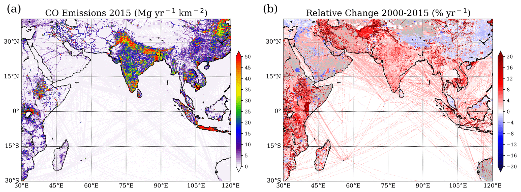
Figure 2 Annual mean CO emissions for 2015 (a) and relative change with respect to 2000 (b) from EDGAR V5.0_AP.

We use the latest versions of the Emissions Database for Global Atmospheric Research (EDGAR) to present continental pollution and greenhouse gas emissions over the last 2 decades. For air pollutants, EDGAR v5.0_AP for the period 1970–2015 is available (Crippa et al., 2020), and for greenhouse gases EDGAR v5.0_GHG for the period 1970–2015 (Crippa et al., 2019a) can be used. The EDGAR datasets include continental emissions from the energy sector (i.e., power industry), industrial processes (i.e., manufacturing, industrial combustion), the transport sector (i.e., road transport, aviation), residential sources (small-scale combustion and waste treatment), and agriculture. Exhausts from ship engines as one of the major sources of air pollution over the open ocean are also included in the EDGAR emissions. The datasets are given at a high spatial resolution of 0.1^∘ × 0.1^∘. The results shown in this section focus on the main pollutants CO, NO_x, and SO₂ and the greenhouse gases CH₄, N₂O, and CO₂. We also briefly discuss mercury emissions. The most recent year for which data are given (the year 2015 for both air pollutants and greenhouse gases) is used here to present emission strength and patterns representative for the last decade. Emission changes are calculated for the time period 2000–2015 and are shown in relative terms compared to the emissions in 2000. Emissions are averaged over East Africa, the Middle East, South Asia, East Asia, and Southeast Asia for a direct comparison of the regional contributions as well as the text and tables.

The ocean is an important source and sink to and from the atmosphere for many of the same gases mentioned above, as well as other climate-active and chemically active compounds, such as DMS, isoprene, and halogen species. Below we will describe the net ocean fluxes of CO, CH₄, CO₂, N₂O, VOCs, DMS, isoprene, and CHBr₃ as obtained from recent publications, placing special attention on monsoon-related variability.

4.1 Pollutants

Among atmospheric pollutants, CO is considered to be one of the most important gases as it is highly toxic at elevated concentrations. Due to its intermediate lifetime of a few months (Seinfeld and Pandis, 2006), CO is much more variable in the troposphere than other atmospheric constituents with longer lifetimes and is often used as a transport tracer. CO has an indirect radiative effect, since it scavenges the hydroxyl radical (OH), the cleaning agent of the atmosphere that would otherwise destroy the greenhouse gases CH₄ and O₃ (Daniel and Solomon, 1998). Another important pollutant is the family of nitrogen oxides (NO_x) consisting of nitrogen dioxide (NO₂) and nitrogen oxide (NO). Tropospheric NO_x acts as a precursor for a number of harmful secondary air pollutants such as ozone and particulate matter and plays a role in the formation of acid rain. Breathing in raised levels of NO₂ can cause respiratory problems independently of negative health effects of other secondary pollutants. SO₂ is another key component of gaseous air pollution. As for NO₂, exposure to SO₂ can harm the human respiratory system. In addition, SO₂ can react with other compounds in the atmosphere to form small particles that contribute to particulate matter pollution. If oxidized within airborne water droplets, SO₂ produces sulfuric acid, which can be transported by wind over many hundreds of kilometers and deposited as acid rain. Atmospheric NH₃ is a pollutant which plays an important role in the formation of particulate matter, as well as in acidification and eutrophication of ecosystems (Lelieveld et al., 2015; Bauer et al., 2016).

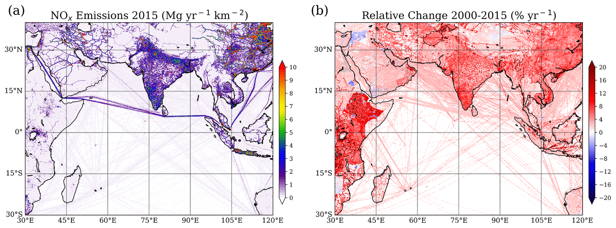
Figure 3 Annual mean NO_x emissions for 2015 (a) and relative change with respect to 2000 (b) from EDGAR V5.0_AP.

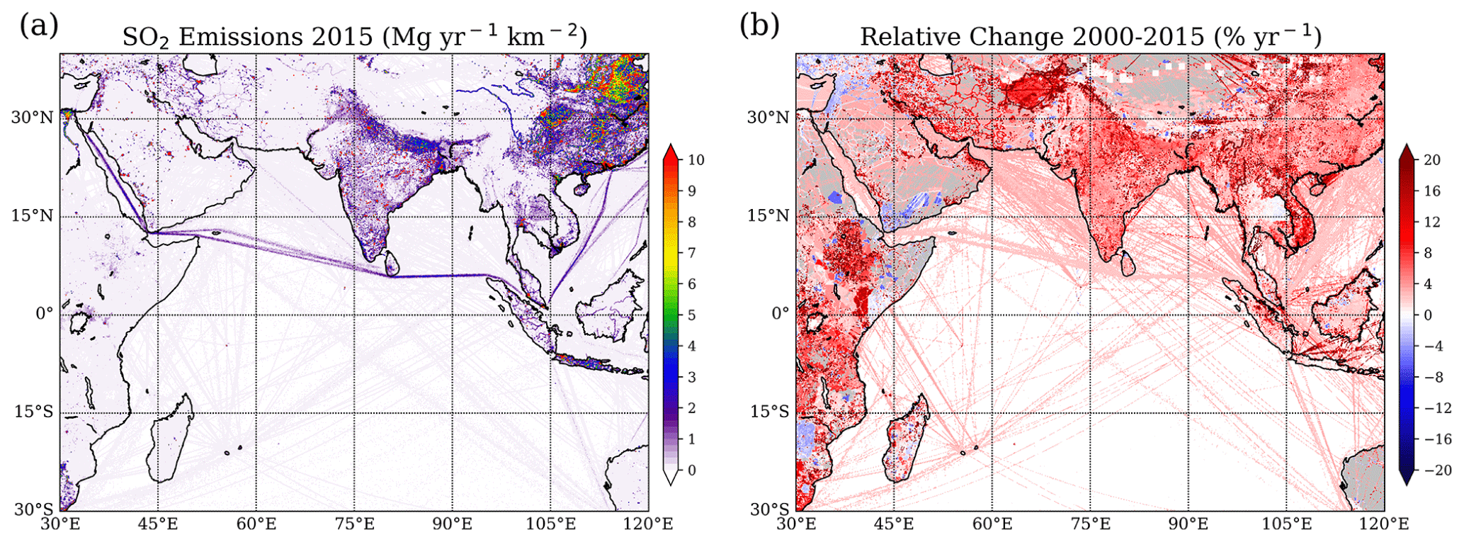
Figure 4 Annual mean SO₂ emissions for 2015 (a) and relative change with respect to 2000 (b) from EDGAR V5.0_AP.

The distributions of CO, NO_x, and SO₂ emissions are shown in Figs. 2, 3, and 4, respectively. One of the common features of the spatial distribution of these emissions is that they generally coincide with the population distribution such that high emissions appear in densely populated areas. In East Asia, high-emission areas include northern China, the Yangtze River delta, Sichuan Basin, and Korea. In South Asia, high emissions are distributed throughout northern India, Nepal, the southern point of India, and Bangladesh. In Southeast Asia, high emissions appear around some major cities including Bangkok, Hanoi, and Ho Chi Minh City, as well as Java. Similar to Southeast Asia, high-emission regions in East Africa are also around major cities like Kampala, Nairobi, and Addis Ababa. In the Middle East, high-emission regions are distributed around the Persian Gulf. Among the different source regions, East Asia and South Asia are main emitters. In 2015, the two regions accounted for 41 % (East Asia) and 27 % (South Asia) of the total CO emissions discussed here. East Asia is also a large emitter of NO_x (54 %) and SO₂ (57 %).

It is well known that pollution sources from Asia are characterized by inefficient combustion processes during biofuel and fossil fuel burning. For instance, the burning of biofuels such as wood, dung, and agricultural waste accounts for 18 % of all CO emissions in Southeast Asia. Globally it only accounted for ∼ 9 % of all CO emissions in 2015, highlighting the role of biofuel burning in regions around the Indian Ocean. Inefficient combustion processes also occur during fossil fuel burning at lower temperatures and result in relatively low NO_x emissions and higher CO $/$ CO₂ ratios when compared to other industrialized areas around the globe. Incomplete fossil fuel combustion from the residential sector and road transportation are the two main sources contributing to CO production, accounting for 29.5 % and 29.0 % of all CO emissions in our study region in 2015.

NO_x emissions mainly stem from high-temperature combustion. Energy production, manufacturing industries, and road transportation caused 30.7 %, 25.8 %, and 25.6 % of all NO_x emissions in our study region in 2015, respectively. Manufacturing industries and energy (electricity and heat production) are also the two main contributors to SO₂ emissions, accounting for 41 % and 40 %, respectively, of all SO₂ emissions in our study region in 2015. As per the 2000 Asian emission inventory, India has the second-highest SO₂ emission (14 %) after China (65 %) with coal-burning power plants contributing to around half (47 %) of the emissions in India (Kurokawa et al., 2013). About 40 % of the thermal plants in India are located over the Indo-Gangetic Plain, causing relatively high SO₂ emissions from this region (Fig. 4; Aswini et al., 2020). In addition, ship traffic leads to anthropogenic NO_x and SO₂ emissions directly over the open ocean with emissions concentrated along the major shipping lanes (e.g., Franke et al., 2009). In general, NO_x ship emissions can lead to substantial ozone enhancements and in turn to higher OH concentrations (Endresen et al., 2003).

Table 2 Emissions of CO, NO_x, and SO₂ from different regions in 2015 and their increase with respect to 2000.

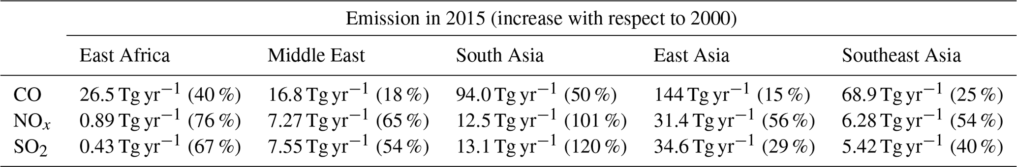
Over the period 2000–2015, the emissions of all pollutants increased in almost all regions around the Indian Ocean, with CO emissions changing from 275.9 to 350.3 Tg yr⁻¹, NO_x from 35.3 to 58.3 Tg yr⁻¹, and SO₂ from 41.8 to 61.1 Tg yr⁻¹. Between 2000 and 2015, CO emissions particularly increased along the Mekong River, north of the Persian Gulf, in Afghanistan, and in East Africa, while CO emissions in most regions of East Asia decreased despite a comparably low overall increase (15 %, Table 2, Fig. 2b). NO_x emission increases show a different pattern and are relatively high in most regions around the Indian Ocean, with peaks in East Asia, South Asia, and East Africa (Fig. 3b). SO₂ emission changes show a similar distribution as the NO_x changes, with peaks along the Mekong River and in East Africa (Fig. 4b). Ship traffic in the Indian Ocean saw the largest increase worldwide between 1992 and 2012, especially on well-defined shipping lanes, such as the Red Sea–Arabian Gulf–Asia route or the Asia–Cape Town route (Tournadre, 2014). The overall increase in pollutant emissions shows pronounced variations from region to region (Table 2), with the highest rate of increase in emissions for all three pollutants found in South Asia.

In particular, for the time period after 2012, satellite measurements have shown pronounced regional SO₂ and NO₂ pollution changes. A decrease in SO₂ pollution from the North China Plain has been noted since 2011 as a result of government efforts, while SO₂ and NO₂ emissions from India have continued to grow at a fast rate (Krotkov et al., 2016). Recent emission estimates suggest that during 2013–2017, anthropogenic emissions from China decreased by 23 % for CO, 21 % for NO_x, and 59 % for SO₂ as a consequence of the implementation of active clean air policies (Zheng et al., 2018).

Unfortunately, measurements of oceanic CO emissions from the Indian Ocean are sparse. We only know of unpublished datasets (D. Arevalo-Martinez, personal communication) from one GEOMAR campaign (OASIS) and a series of NASA–SAGA cruises (https://gml.noaa.gov/hats/ocean/, last access: 1 July 2021, eastern open Indian Ocean, summer 1987). Net fluxes covering the northern to southern extent of the Indian Ocean range from ∼ 0.1 to ∼ 1.4 Mg km⁻² yr⁻¹, as CO is always supersaturated in the surface ocean (Conte et al., 2019, and references therein). These values are similar to ship emissions but considerably smaller than continental emissions (Fig. 2). CO is produced in the surface ocean from organic material photochemistry and biological processes (Conte et al., 2019). Available data from the western Indian Ocean suggest that the most significant meridional gradients occur due to open-ocean upwelling at 5–10^∘ S. CO emissions are high from 5–15^∘ S, but to the north and south of this region, emissions decrease to zero with seasonal variations occurring due to upwelling changes. In the eastern Indian Ocean, seasonal variability is expected in association with surface productivity changes in the Seychelles–Chagos thermocline ridge. However, no seasonal cycle can be detected in available measurements from this region, and it is not clear if this is a real feature or caused by the lack of data. Additional variability is expected in coastal regions, since large amounts of seasonally discharged runoff supply terrestrial organic material that serves as a precursor to CO marine photoproduction.

The atmospheric pollutant mercury is transported around the globe as gaseous elemental mercury, eventually oxidizing to divalent mercury. The latter is known to deposit to the surface from where it can be taken up into food webs and transformed to highly toxic species endangering humans and ecosystems (Selin et al., 2007). Atmospheric mercury is released from anthropogenic activities, such as coal-fired power plants, metal smelting, and waste incineration (Pacyna and Pacyna, 2005; Streets et al., 2005). Emissions associated with artisanal and small-scale gold mining account for almost 38 % of the global total emission (UN-Environment, 2019). Mercury is also emitted from the oceans, soils, terrestrial vegetation, and biomass burning. These mostly natural emissions include some anthropogenic fraction related to the recycling of previously deposited mercury (Mason and Sheu, 2002). Based on 2015 inventories, Asia is responsible for a large part of the emissions (49 %), which primarily stem from East and Southeast Asia. While emissions in North America and the European Union have shown moderate decreases, increased economic activity, notably in Asia, and the use and disposal of mercury-added products led to a global increase of approximately 20 % between 2010 and 2015 (UN-Environment, 2019).

For NH₃, East Asia and South Asia are the two main contributors, which account for 38.9 % and 32.3 % of the total emissions, respectively (not shown here). From 2000 to 2015, emissions of NH₃ in the regions around the Indian Ocean documented by EDGAR increased by 22.5 %. Agricultural activities dominate the ammonia emissions, with about 56.7 % and 18.4 % of the emissions coming from direct soil emission and manure management. Besides, long-term satellite measurements (van Damme et al., 2018) show other hotspots of ammonia emission not well represented in the EDGAR inventory, most of which are associated with either high-density animal farming or industrial fertilizer production.

4.2 Greenhouse gases

CO₂ concentrations have been increasing steadily over the last decades, reaching a new annual global mean record high in 2020 of 412.5 ± 0.1 ppm​​​​​​​ (Blunden and Boyer, 2020). Due to its high atmospheric abundance and long atmospheric lifetime, CO₂ is the most important of Earth's long-lived greenhouse gases. In addition to its impact on climate, CO₂ is responsible for ocean acidification as it produces carbonic acid when it dissolves in the ocean. CH₄ is also a very effective greenhouse gas and the second-largest contributor to anthropogenic radiative forcing since preindustrial times after CO₂. In the troposphere, CH₄ acts to reduce the atmosphere's oxidizing capacity. It has a relatively short atmospheric lifetime of about 12.4 years (Myhre et al., 2013) and exhibits a strong seasonal cycle as well as a distinct gradient across the Equator. Despite its relatively low atmospheric concentrations, N₂O is the third anthropogenic greenhouse gas after CO₂ and CH₄ in terms of radiative forcing (Ciais et al., 2014). Due to its long atmospheric lifetime of about 116 years (Prather et al., 2015) and large infrared absorption capacity per molecule, N₂O is a much more efficient greenhouse gas than CO₂ with a global warming potential of 265 over a 100-year time span. In the stratosphere, reaction with O(¹D) leads to the production of NO (Seinfeld and Pandis, 2006), which is involved in chemical ozone depletion. As a consequence, N₂O has been estimated to be the main emitted ozone-depleting substance of the 21st century (Ravishankara et al., 2009; Butler et al., 2016).

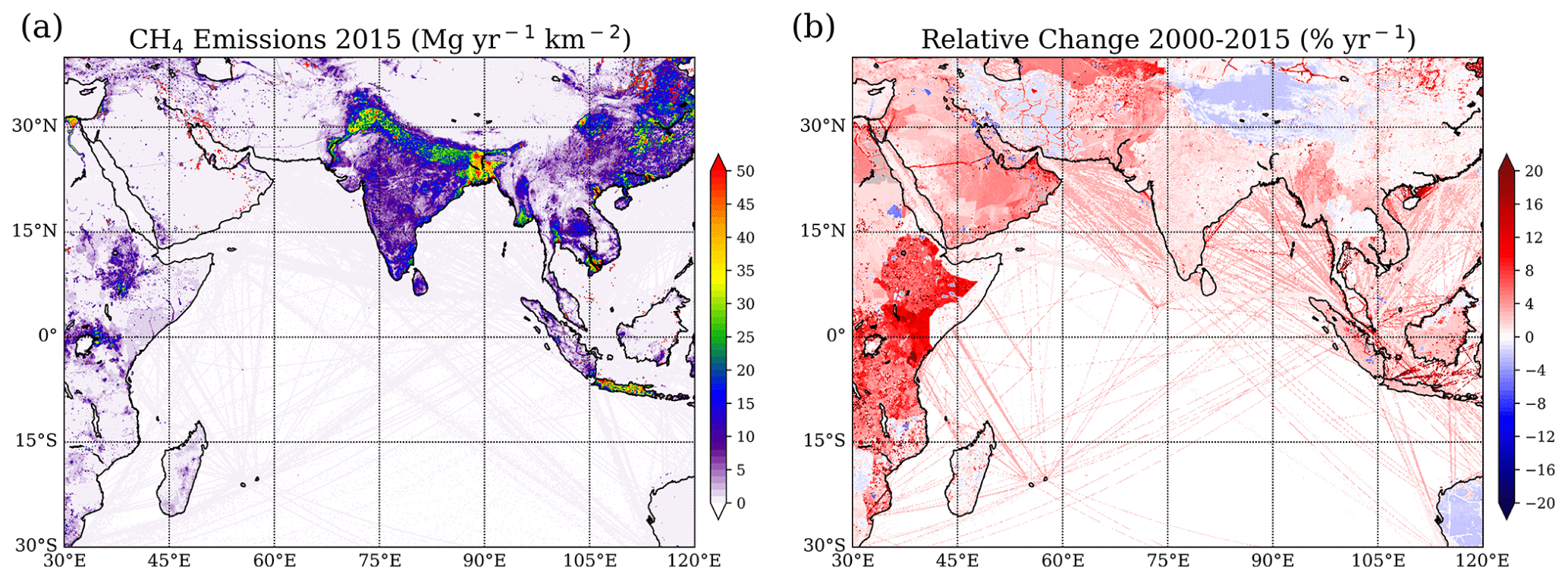
Figure 5 Annual mean CH₄ emissions for 2015 (a) and relative change with respect to 2000 (b) from EDGAR V5.0_GHG.

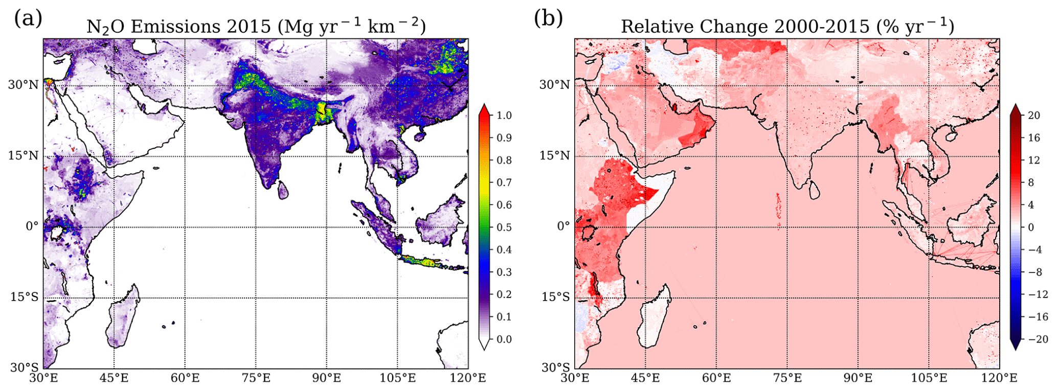
Figure 6 Annual mean N₂O emissions for 2015 (a) and relative change with respect to 2000 (b) from EDGAR V5.0_GHG.

Anthropogenic greenhouse gas emissions in the regions surrounding the Indian Ocean generally correspond to economic activities. As the largest emerging economies, East Asia and South Asia are the main emitters of CH₄ (Fig. 5) and N₂O (Fig. 6) with emission centers in the Indo-Gangetic Plain, northern China, and Java. In 2015, East Asia and South Asia accounted for 37 % and 26 % of the total CH₄ emission, as well as 43 % and 26 % of the total N₂O emission discussed here. Among the regions surrounding the Indian Ocean, East Asia is also the largest CO₂ emitter, causing 68 % of the total CO₂ emissions in our study region in 2015 (Fig. 7).

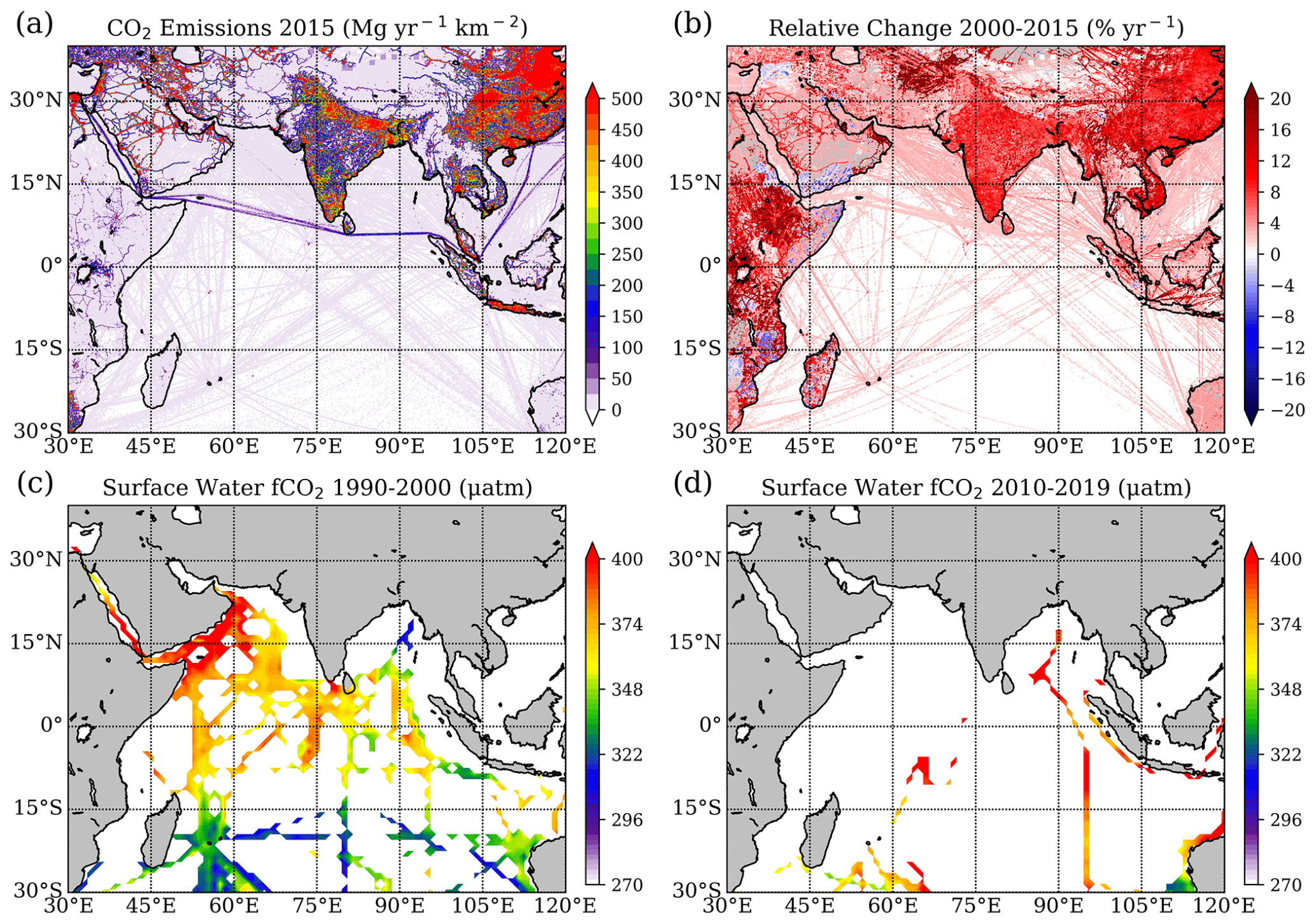
Figure 7 Annual mean CO₂ emissions for 2015 (a) and relative change with respect to 2000 (b) from EDGAR V5.0_GHG. Surface water fCO₂ observations (color shading, unit: µatm) over the Indian Ocean for 1990–2000 (c) and 2010–2019 (d) from SOCATv2019.

Atmospheric CH₄ has anthropogenic and natural sources, with the latter including natural wetlands, livestock, termites, hydrates, and forest fires. Anthropogenic sources account for the majority of all emissions and can be split into biogenic and non-biogenic sectors. Almost a quarter (23 %) of the CH₄ emissions in our study region stems from enteric fermentation (livestock farming), which acts as the primary source in South Asia and East Africa. Rice cultivation in Asia is responsible for 19 % of CH₄ emissions in our study region, causing a systematic seasonal pattern with peak emissions during the fully grown stage in September and October (Pathak et al., 2005). Other main sources of CH₄ are solid fuels (17 %), mainly from East Asia and Southeast Asia, and oil and gas production (14 %), mainly from the Middle East.

N₂O emissions are linked to the biogeochemical cycle of nitrogen and are thus impacted by anthropogenic use of fertilizer and industrial activities that lead to the atmospheric deposition of reactive nitrogen (e.g., Davidson, 2009). More than half of the N₂O emissions in our study region (56 %) are directly from managed soils and can be quite heterogeneous, with spatial patterns revealing hotspots in agricultural areas in China and the Indo-Gangetic Plain (Ito et al., 2018; Fig. 6). Furthermore, the N₂O emissions from managed soils are characterized by a pronounced seasonal cycle and interannual variability, primarily in response to meteorological conditions and nitrogen inputs. In particular, N₂O emissions are correlated with soil moisture (Raut et al., 2015), leading to strongly enhanced emissions in South Asia during summertime when high-precipitation events occur.

Table 3 Emissions of CH₄, N₂O, and CO₂ from different regions in 2015 and their increase with respect to 2000.

Similar to the air pollutants discussed above, the overall CH₄ and N₂O emissions increased significantly over the period 2000–2015 from 135.7 to 182.4 Tg yr⁻¹ and from 2.80 to 3.51 Tg yr⁻¹, respectively. Increasing CH₄ emissions in South Asia (Fig. 5b) have been linked to increased rice cultivation area, natural wetlands, and warmer climate (Tian et al., 2015). Increasing N₂O emissions (Fig. 6b) are believed to stem from intensified crop production and nitrogen fertilizer use as well as higher air temperatures (Raut et al., 2015). While not being the main emitter, East Africa is the region with the fastest increase in CH₄ and N₂O emissions among the regions discussed here (Figs. 5b and 6b, Table 3). A recent study suggested that East African wetlands could account for up to a third of the spike in global CH₄ emissions between 2010 and 2016, with most of this coming from the South Sudanese wetland, one of the largest freshwater ecosystems in the world (Lunt et al., 2019).

For CO₂, the majority of the emissions in our study region stem from East Asia related to two main sectors: electricity and heat production (41 %) and manufacturing industries (23 %). Over the period 2000–2015, the CO₂ emissions in our study region more than doubled from 8790 to 19168 Tg yr⁻¹. Especially in East Asia and South Asia, they grew at very fast rates with increases of 127 % and 125 %, respectively. Despite the apparent policy breakthrough leading to the Paris Agreement in 2015, CO₂ emissions from fossil fuel and industry have continued to increase over the recent years. According to the latest estimates from the Global Carbon Project, the expected growth of global emissions in 2019 will be almost entirely due to China and India, with expected annual growth rates of 2.6 % and 1.8 %, respectively (Peters et al., 2020).

The ocean is also a source and sink of greenhouse gases. Compared to the terrestrial sources, the ocean is just a minor contributor to atmospheric CH₄, accounting for 1 %–13 % of the global atmospheric CH₄ budget (Saunois et al., 2016). The concentration of CH₄ in the Indian Ocean is characterized by a sharp decrease offshore (Naqvi et al., 2010a). Due to the large geographical changes in surface saturation and wind speed, the air–sea flux of CH₄ varies strongly in the northern Indian Ocean. The highest emissions were observed during the southwest monsoon in the Arabian Sea (∼ 64 µmol m⁻² d⁻¹), and the estimated overall CH₄ emission from the Arabian Sea amounts to 0.1–0.2 Tg yr⁻¹ (Naqvi et al., 2005), which is much smaller than the total terrestrial emissions mentioned above (∼ 182 Tg yr⁻¹ in 2015).

Unlike CH₄, the ocean is a major source of N₂O, accounting for at least one-third of global N₂O emissions (Bange, 2006). Intense N₂O emissions are usually found in upwelling regions with OMZs (Codispoti, 2010), such as in the Arabian Sea and Bay of Bengal (not shown). The South Asian monsoon drives intense seasonal changes in upwelling in both OMZs, thus affecting the regional N₂O productivity and emissions. The upwelling in the Arabian Sea is most intense during the South Asian summer monsoon, leading to high oceanic N₂O production (Naqvi et al., 2010a) and emissions of 0.34–0.99 Tg N₂O yr⁻¹ (Naqvi et al., 2010b), representing 2 %–31 % global oceanic N₂O emissions (Suntharalingam et al., 2019). However, the estimate by Sudheesh et al. (2016) in the southeastern Arabian Sea, based on measurements from Mangalore and Kochi, is almost 4 times lower than previous estimates. Raes et al. (2016) proposed that the southeastern Indian Ocean could be both a source and sink of N₂O, suggesting great uncertainty of the oceanic emission of N₂O in the Indian Ocean. The upwelling driven by the summer monsoon also occurs in the Bay of Bengal; however, it is attenuated by the intense precipitation and pronounced freshwater discharge from the Ganges, yielding lower N₂O productivity (Singh and Ramesh, 2015) and much smaller emission (∼ 0.03–0.11 Tg N₂O yr⁻¹, Naqvi et al., 1994, 2010b). There is some indication that increased nitrogen deposition, due to anthropogenic perturbation, already influences the air–sea flux of N₂O in the northern Indian Ocean and will continue to do so into the future (Suntharalingam et al., 2019). Due to sparse measurements, it is impossible to compare the oceanic N₂O emission of the Indian Ocean with the terrestrial emissions directly. However, the emissions from the Arabian Sea alone are about 9.6 %–28 % of the terrestrial emissions of the study region (∼ 3.5 Tg yr⁻¹ in 2015), suggesting the importance of the oceanic source in the Arabian Sea region. Enhanced N₂O air–sea fluxes were also found in a zonal band between 5 and 10^∘ S as a result of wind-driven upwelling during the OASIS research cruise in 2014 (Ma et al., 2018).

While the global oceans act as a net sink of CO₂, absorbing about 25 % of the annual anthropogenic CO₂ emission (Le Quéré et al., 2018), the air–sea exchange of CO₂ varies at different spatial and temporal scales. The northern Indian Ocean is a net source of CO₂ to the atmosphere, while the southern Indian Ocean is a net sink (e.g., Sarma et al., 2013). Based on the inorganic carbon data collected in the Indian Ocean in 1995, for example, Bates et al. (2006) suggested that the Bay of Bengal is a net oceanic source of atmospheric CO₂. Takahashi et al. (2009) constructed the climatological mean distribution for the sea surface water pCO₂ over the global oceans based on observations from 1970 and 2007, and they suggested that the Bay of Bengal is near equilibrium for CO₂. By examining numerical results produced by various ocean biogeochemical models and different atmospheric inversions, Sarma et al. (2013) argued that the Bay of Bengal is a small annual net sink region for atmospheric CO₂. Other studies report that on an annual scale, specific regions in the Bay of Bengal emit between ∼ 1.61 and 2.45 ± 0.49 Mg CO₂ yr⁻¹ km⁻² (Dixit et al., 2019; Ye et al., 2019). Significant impacts of tropical cyclones (Ye et al., 2019), biological productivity (Chakraborty et al., 2018), and freshwater discharge (Sarma et al., 2011) on the CO₂ air–sea exchange have been suggested for the Bay of Bengal. If compared to anthropogenic emissions of more than 500 Mg CO₂ yr⁻¹ km⁻² over large areas (Fig. 7a), the contribution of the northern Indian Ocean to atmospheric CO₂ is relatively low. Analyzing the Surface Ocean CO₂ Atlas (SOCATv2019; Bakker et al., 2016) demonstrates that in the Indian Ocean only a few CO₂ measurements are available for the last decade, especially when compared with the 1990s (Fig. 7c and d), making it impossible to assess the long-term changes in CO₂ air–sea exchange in this region. Northern Indian Ocean CO₂ flux variability may be influenced by El Niño–Southern Oscillation (ENSO) events (Valsala and Maksyutov, 2013) and hydrographic features (i.e., eddies; Valsala and Murtugudde, 2015).

During the OASIS campaign in the western Indian Ocean (Zavarsky et al., 2018a), both positive and negative CO₂ fluxes were observed based on the direct eddy covariance flux technique. South of the Equator, average values were 0.2 and −0.28 Mg d⁻¹ km⁻², respectively, making this region a net sink of CO₂. These results are consistent with Chen et al. (2011), who found significant spatial and temporal variability in the southern Indian Ocean carbon sink. However, by comparing campaigns that occurred from 1999–2000 to those from 2004–2005, Chen et al. (2011) deduced that the sink of the southern Indian Ocean is weakening. A decadal variability analysis from 1991–2007 of dissolved CO₂ in surface seawater in the southern Indian Ocean (20–55^∘ S) suggests that it increased at a faster rate than atmospheric CO₂ (Metzl, 2009), indicating that the ocean carbon sink weakened. The authors suggested that the reduction was related to variability in the Southern Annular Mode. The weakening of Indian Ocean carbon sink has also been found in a recent modeling study (DeVries et al., 2019). The southern Indian Ocean CO₂ fluxes are driven by both the solubility and biological pumps, with indications of decadal variability (Valsala et al., 2012).

Carbonyl sulfide (COS) is another important long-lived trace gas that acts as a greenhouse gas in the troposphere and as the main precursor of aerosols in the stratosphere (Brühl et al., 2012; Kremser et al., 2016). The ocean is the main source of COS to the atmosphere globally, previously estimated at 441–542 Gg COS yr⁻¹, but a revision of the vegetation sinks has led to the hypothesis that the ocean source might be stronger than previously calculated. The missing ocean source is hypothesized to be in the tropics (e.g., Suntharalingam et al., 2008; Glatthor et al., 2015). Launois et al. (2015) modeled oceanic concentrations and emissions for this region that are approximately an order of magnitude higher, but the values do not agree with the albeit sparse COS measurements that exist in the Indian Ocean. A recent measurement and modeling study on the OASIS campaign has shown that, in fact, the ocean source of COS is not higher than previously determined (Lennartz et al., 2017). Daily integrated air–sea fluxes computed for the southern Indian Ocean ranged between −0.045 and −0.000375 g COS km⁻², indicating that the Indian Ocean may be a net sink for COS. In addition, COS is produced in the atmosphere from DMS and carbon disulfide (CS₂) oxidation, both of which are emitted from the ocean (Chin and Davis, 1993; Watts, 2000). These pathways increase the ocean source of COS indirectly but do not account for the full missing ocean source (Lennartz et al., 2017). Campbell et al. (2015) and Lennartz et al. (2017) point to anthropogenic emissions of COS from Asia to close the gap, and indeed Lee and Brimblecombe (2016) find twice as much COS in the atmosphere from anthropogenic emissions than previously thought. They report that anthropogenic COS emissions account for approximately one-third of global emissions and originate from the paper industry as well as biofuel and coal combustion. Another study suggests that COS emission from domestic coal combustion only in China would be at least 57.2 ± 10.5 Gg COS yr⁻¹, which is an order of magnitude greater than recent estimates of COS emissions from the total coal combustion in China (Du et al., 2016).

4.3 VOCs and short-lived gases DMS, isoprene, and bromoform

4.3.1 Volatile organic compounds (VOCs)

Volatile organic compounds (VOCs), such as alkanes, alkenes, and alkynes, are highly reactive throughout the troposphere, influencing oxidants (OH, O₃, NO₃) (Williams et al., 2010), and peroxyaceylnitrate (PAN), which is a reservoir for reactive nitrogen compounds, and forming secondary organic aerosols (SOA) (Singh et al., 1995; Blando and Turpin, 2000). Oxygenated VOCs play a special role in upper-tropospheric OH production (e.g., Singh et al., 1995).

The Middle East is a hotspot of VOC emissions, such as ethane and propane, from oil and gas production. Interestingly, a recent study found that deep water masses can be a large source of VOCs comparable with total anthropogenic emissions from individual Middle Eastern countries (Bourtsoukidis et al., 2020). Other biogenic sources of VOCs include surrounding forested areas (Duflot et al., 2019). Formaldehyde (HCHO) is emitted via biomass burning and fuel combustion. In addition, it has a secondary source via reactions between OH and CH₄. Ship fuel combustion has recently been targeted as a large source (Gopikrishnan and Kuttippurath, 2021). This was first postulated by Marbach et al. (2009) using satellite measurements of HCHO and shown again by De Smedt et al. (2021).

In addition to the Bourtsoukidis et al. (2020) study cited above, the Indian Ocean has been shown to be a main source of VOCs at other specific locations, such as at the Maïdo Observatory (Duflot et al., 2019). Evidence of alkene emissions from the Indian Ocean and specifically the Bay of Bengal was presented by Sahu et al. (2010, 2011) by demonstrating that the ratios of ethene $/$ propene are in line with fresh oceanic emissions (2.3 ppt ppt⁻¹). Alkene emissions seem to be controlled by dissolved organic carbon, wind speed, and sunlight. The eastern Indian Ocean may be a source of biogenic VOCs, leading to the production of acids (diacids, oxocarboxylic acids, and α-dicarbonyls) in the atmosphere (Yang et al., 2020). The highly productive Arabian Sea OMZ area has been associated with enhanced production of alkanes and alkenes related to Trichodesmium and Thalassiosira phytoplankton species (Tripathi et al., 2020).

4.3.2 Dimethylsulfide (DMS)

Marine DMS is the largest source of biogenic sulfur to the atmosphere. DMS is produced from the algal-derived precursor dimethylsulfoniopropionate (DMSP), which is cleaved by marine microbes to form DMS. Only a small fraction of this DMS is released to the atmosphere. The seminal CLAW hypothesis proposed a feedback loop between marine biogenic DMS production, emissions, and climate via aerosol and cloud formation (Charlson et al., 1987), triggering decades of research on DMS cycling in the ocean and emission to the atmosphere. Lana et al. (2011) present the most comprehensive and up-to-date monthly DMS concentration and flux climatology resulting from this large body of research. Unfortunately, measurements in the Indian Ocean are sparse and most values in the climatology are interpolated, with only 6271 non-uniformly spaced data points over 40 years available in the Indian Ocean.

Figure 8 DMS emissions for (a) summer monsoon (June–August), (b) winter monsoon (December–February), (c) spring transition (April–May), and (d) autumn transition (October) from Lana et al. (2011).

DMS emissions exhibit clear seasonality, with the highest fluxes basin-wide evident during the summer monsoon period. According to Lana et al. (2011), the summertime values in the Indian Ocean are a global hotspot for DMS emissions. The largest values are found in the Arabian Sea (Fig. 8). High biological productivity associated with the upwelling areas off northeastern Africa and the Arabian Sea are strongly correlated with the monsoon cycle (Yoder et al., 1993). Combined with the strong, steady winds during the summer monsoon, fluxes of DMS reach their peak. The lowest fluxes are computed during the spring transition period, likely associated with low productivity and low wind speeds. Year-round, there is a relatively large flux area around 15^∘ S, which migrates north and south according to the summer hemisphere and is related to biogenic processes in the upwelling. Winds are always relatively high in this region throughout the year (Fig. 1), which also enhances the flux. Maximum emissions of over 650 kg DMS km​​​​​​​⁻² yr⁻¹ for the Arabian Sea (Lana et al., 2011) translate to slightly larger S flux to the atmosphere from DMS than that from SO₂ ship emissions (approximately 335 kg S km⁻² yr⁻¹ from DMS and 250 kg S km⁻² yr⁻¹ from SO₂).

Galí et al. (2018) used satellite-based proxies to estimate the DMS concentration climatology and reported that the Lana et al. (2011) climatology overestimates DMS in the Indian Ocean region by 25 %–50 % during all seasons. DMS direct flux measurements using the eddy covariance technique and ocean concentration measurements were performed during the OASIS campaign in order to compare directly with the Lana climatology in the western tropical Indian Ocean (Zavarsky et al., 2018a). The oceanic DMS concentrations were found to be lower than those in the climatology, but the difference was more pronounced south of 16^∘ S where measured values were a third of those in the climatology. North of 16^∘ S, the measured ocean concentrations were in better agreement with those in the climatology until the vicinity of the Maldives, where they were again lower by a factor of 3. The measured fluxes were subsequently lower than the climatology for the region by approximately 60 % on average. This was attributed to lower measured oceanic concentrations, as well as lower measured wind speeds than used in the climatology and a different gas transfer parameterization. The directly derived gas transfer parameterization was linearly dependent on wind speed, while the climatology uses a quadratic wind speed dependence. Nonetheless, the Indian Ocean appears to be a hotspot for DMS emissions during the summer monsoon, likely with a sulfur loading to the atmosphere on the order of half of that from SO₂ ship emissions.

4.3.3 Isoprene

Isoprene (2-methyl-1,3-butadiene) is a biogenic VOC and accounts for half of the total global biogenic VOCs in the atmosphere (Guenther et al., 2012). Most is emitted from terrestrial vegetation (400–600 Tg C yr⁻¹, Guenther et al., 2006; Arneth et al., 2008). The ocean source strength is much lower, and the magnitude is debated (Carlton et al., 2009), with most estimates lower than 1 Tg C yr⁻¹ (Palmer and Shaw, 2005; Arnold et al., 2009; Gantt et al., 2009; Booge et al., 2016). It is known from laboratory studies that phytoplankton produce isoprene (Exton et al., 2013, and references therein), but only a few studies have performed direct measurements of marine isoprene concentrations worldwide.

Emitted isoprene affects the oxidative capacity of the atmosphere through ozone and OH interactions and is a source for SOAs (Carlton et al., 2009). Due to the short atmospheric lifetime of minutes to a few hours, terrestrial isoprene does not reach the atmosphere over much of the ocean. Therefore, marine emissions of isoprene could play an important role in SOA formation on regional and seasonal scales, especially in association with increased production during phytoplankton blooms (Hu et al., 2013). Furthermore, isoprene SOA yields increase under acid-catalyzed particle-phase reaction in low-NO_x conditions, which dominate over open-ocean regions (Surratt et al., 2010) and are significantly higher than during neutral aerosol experiments (Henze and Seinfeld, 2006). Here we provide data from a published modeling study from the OASIS campaign with input variables from 2014 to assess seasonal isoprene fluxes to the atmosphere from the Indian Ocean (Booge et al., 2016, 2018).

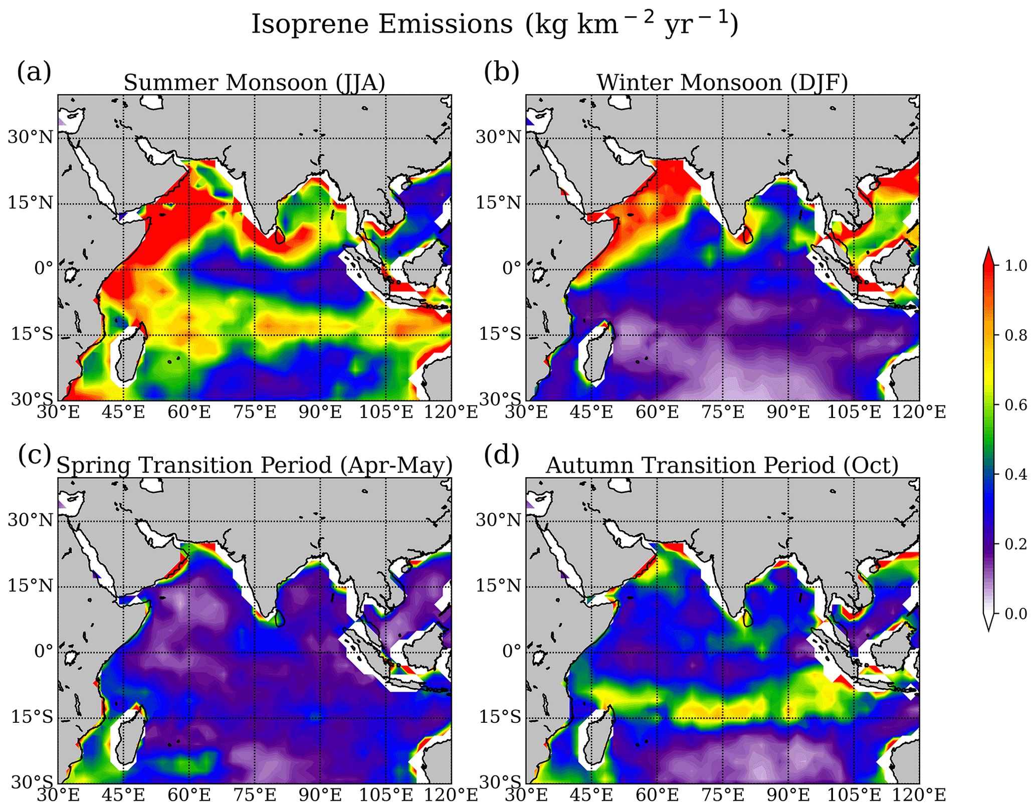
Figure 9 Isoprene emissions for (a) summer monsoon (June–August), (b) winter monsoon (December–February), (c) spring transition (April–May), and (d) autumn transition (October) from Booge et al. (2016).

Isoprene fluxes to the atmosphere change seasonally, with the highest values computed during the summer monsoon over the entire Indian Ocean extent (Fig. 9). The summer values are the second-highest values globally during that season, following the Southern Ocean. The lowest isoprene emissions in the Indian Ocean are found in the spring transition period. This seasonal pattern is similar to the DMS emission pattern. Computed fluxes during the winter monsoon are high in the northern region of the Indian Ocean, especially in the Arabian Sea. A belt of relatively high isoprene fluxes can be seen in the autumn transition period around 15^∘ S, but the values are lower than the highs seen during the summer (basin-wide) and winter (Arabian Sea) monsoon season. Unlike DMS, this is only visible in the summer and autumn seasons. Isoprene production rates are phytoplankton-functional-type dependent and are driven further by light, SST, salinity, and nutrients (Booge et al., 2018). High light and high SST favor higher production, while high salinity and high nutrients lead to lower production. The combination of the direct influence of wind speeds on fluxes and the interaction of the environmental factors and isoprene production leads to the seasonal patterns.

4.3.4 Halogens

Halogenated very short-lived substances (VSLSs, with lifetimes shorter than 6 months) from the ocean, such as bromoform (CHBr₃), dibromomethane (CH₂Br₂), and methyliodide (CH₃I), contribute to atmospheric halogen loading and ozone depletion (Engel and Rigby, 2018). The oceanic CHBr₃ surface concentrations are spatially and temporally highly variable. Natural production of CHBr₃ involves marine organisms such as macroalgae and phytoplankton (Gschwend et al., 1985), while CH₂Br₂ is formed in parallel and correlates with CHBr₃ in water and air (Tokarczyk and Moore, 1994). A recent study suggests that heterotrophic processes in the ocean can increase the flux of CH₂Br₂ from the sea to the atmosphere (Mehlmann et al., 2020). Enhanced emissions of brominated VSLSs coincide with biologically active equatorial and coastal upwelling regions (Quack et al., 2007) as well as the distribution of macroalgae and anthropogenic sources along the coasts (Carpenter and Liss, 2000; Maas et al., 2021). Iodinated VSLSs such as CH₃I, on the other hand, show elevated oceanic abundances in the subtropical gyre regions, in agreement with identified production by photochemical reactions (Richter and Wallace, 2004).

Various CHBr₃ emission inventories have been derived from the extrapolation of measurement-based data (Ziska et al., 2013; Fiehn et al., 2017), oceanic modeling (Stemmler et al., 2015), top-down atmospheric modeling approaches (Liang et al., 2010), and a data-oriented machine-learning algorithm (Wang et al., 2019). Overall, large differences between CHBr₃ emission inventories exist with the observation-based, bottom-up emissions (Ziska et al., 2013), being most consistent with atmospheric measurements in the tropics (Hossaini et al., 2013). All inventories agree on the tropical Indian Ocean being a productive source region of CHBr₃.

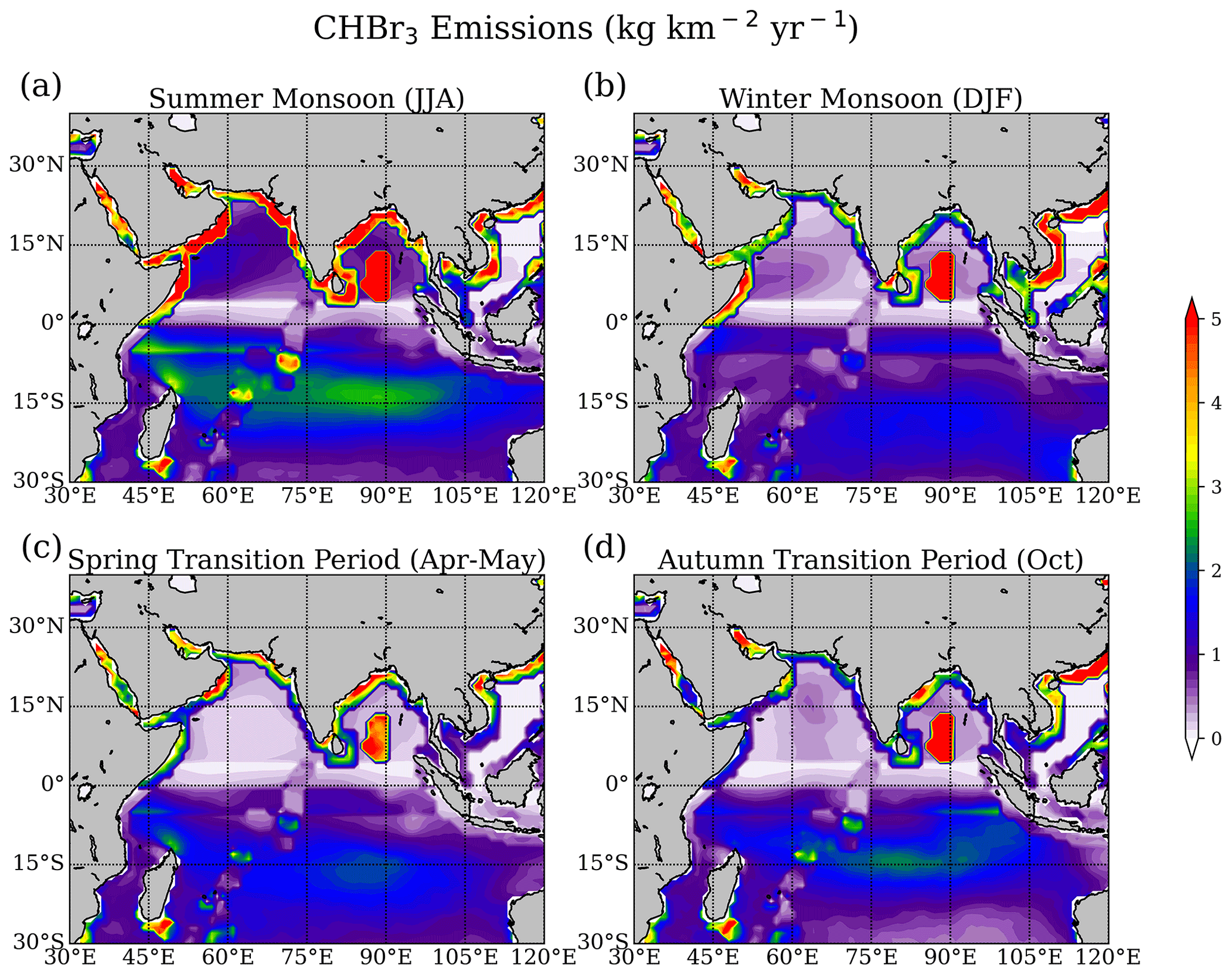
Figure 10 Bromoform (CHBr₃) emission for (a) summer monsoon (June–August), (b) winter monsoon (December–February), (c) spring transition (April–May), and (d) autumn transition (October) based on static surface concentrations and ERA-Interim meteorology for 2014 (Fiehn et al., 2018).

Here we show the most recent bottom-up CHBr₃ emission inventory (Fiehn et al., 2018) based on two campaigns in the marginal seas (Yamamoto et al., 2001; Roy et al., 2011), one campaign in the open Indian Ocean (Fiehn et al., 2017) and extrapolations of measurements from other oceans (Ziska et al., 2013), in Fig. 10. The emission inventory is based on static surface concentration maps generated from atmospheric and oceanic surface ship-borne in situ measurements collected within the HalOcAt (Halocarbons in the ocean and atmosphere) database project (https://halocat.geomar.de, last access: 1 July​​​​​​​ 2020). While the concentration maps do not provide any temporal variability, the emission parameterization is based on monthly mean meteorological ERA-Interim data, allowing for relative emission peaks related to maxima in the horizontal wind and SST.

The CHBr₃ emissions peak along the Northern Hemisphere (NH) coastlines due to macroalgae production and anthropogenic sources (3.3–6.6 kg km⁻² yr⁻¹), the central Bay of Bengal (up to 11.1 kg km⁻² yr⁻¹), and the southern tropical Indian Ocean (2.2 kg km⁻² yr⁻¹). The coastal emissions in the Indian Ocean of the bottom-up inventory presented here agree well with other emission estimates (Fiehn et al., 2018). High emissions along the coasts of Somalia and Oman due to coastal upwelling detected in biogeochemical modeling studies (Stemmler et al., 2015) are not captured here due to missing CHBr₃ measurements in this biogeochemical regime. The emissions show a pronounced seasonal cycle with a peak during the summer monsoon period (Fig. 10) due to higher wind speeds over the whole Indian Ocean during this time of year (Fig. 1).

Once destroyed in the atmosphere, brominated VSLSs contribute to the family of inorganic bromine (Br_y) consisting of bromine radicals such as bromine monoxide (BrO) and non-radical reservoir species such as HBr and HOBr. Inorganic bromine also has other anthropogenic and natural sources including methyl bromide, which is a product of biomass burning, leaded fuel combustion, plant and marsh emissions, and soil fumigation (Manö and Andreae, 1994). Inorganic bromine can also be released when sea salt is exposed to the atmosphere from young sea ice surfaces, frost flowers, snowpack, seawater, and marine aerosols (Hay et al., 2007).

Similar to bromine, inorganic iodine such as iodine oxide (IO) is produced through the degradation of its organic precursor CH₃I and other short-lived iodinated VSLSs. The primary sources of iodine to the marine boundary layer, however, are believed to be inorganic iodine emissions at the ocean surface from reactions of dissolved iodide with deposited gas-phase ozone (Carpenter et al., 2013). Once in the atmosphere, inorganic iodine plays an important role for the boundary layer chemistry by influencing the oxidizing capacity through catalytically removing O₃ and altering the HO_x and NO_x balance.

5 Atmospheric composition

During the South Asian summer monsoon, clean air dominates the atmospheric composition over the Indian Ocean, leading to a completely different chemical regime than observed during wintertime. As the ITCZ moves over the Indian subcontinent (Waliser and Gautier, 1993), air mass transport via steady winds is directed from the ocean towards the land and anthropogenic pollutants are confined to the continents. During this period, the intense summer monsoon rainfall also effectively removes many soluble species from the continental boundary layer. During the winter monsoon and transitional months, the wind pattern is reversed, with continental air masses being transported towards and over the open-ocean environment. This leads to an increase in the anthropogenic origin trace gases and aerosol loading over the Indian Ocean. Based on studies and campaigns that took place before 2010, Lawrence and Lelieveld (2010) provided a comprehensive review of atmospheric composition over the Indian Ocean. Here we summarize their most important findings and report on new datasets and results that have emerged since then.

5.1 Pollution and O₃

The surface distributions of anthropogenic pollutants and ozone levels are often highly correlated as the majority of tropospheric ozone formation occurs when CO, NO_x, and other ozone precursor gases react in the atmosphere in the presence of sunlight. Tropospheric ozone is a greenhouse gas with a relatively short lifetime on the order of several weeks and is therefore considered a near-term climate forcer. The direct radiative forcing of ozone is estimated to be 0.40 ± 0.20 W m⁻² (IPCC, 2013), and additional indirect radiative forcings can result from its impact on vegetation, carbon uptake, and methane lifetime (e.g., Lombardozzi et al., 2015; Fiore et al., 2008). Ozone also acts as an environmental pollutant detrimental to human health, as well as crop and ecosystem productivity (e.g., Monks et al., 2015). Changes in ozone precursor emissions, low-frequency climate variability, and long-term anthropogenic climate change all impact the quantity and distribution of tropospheric ozone (e.g., Barnes et al., 2016).

The distribution and variations of pollutants and ozone over the Indian Ocean have been investigated during individual campaigns (e.g., ICARB) and can be derived from continuous in situ (e.g., ozone profiling at Indian coastal stations) and satellite measurements (e.g., OMI and MOPITT). The various datasets offer different advantages, allowing for a wide range of applications. While the in situ measurements are characterized by higher resolution and lower uncertainties, they are usually limited in space (stations) or time (campaigns). The satellite measurements, on the other hand, offer comprehensive spatial coverage and extend over longer time periods but suffer from limited vertical resolution and higher uncertainties. Most available Indian Ocean campaigns and studies investigate O₃, CO, and NO_x. As a result, the following sections focus on the distribution and variability of these three gases, while SO₂ and mercury are only discussed briefly.

5.1.1 Carbon monoxide (CO) and nitrogen oxides (NO_x)

The distribution of the major pollutant CO over the Indian Ocean is well known from MOPITT satellite measurements (e.g., Ghude et al., 2011; Srivastava et al., 2012a). Seasonal mean surface values for 2014/2015–2018/2019 show a clear gradient between CO over the Indian Ocean and over the landmass source regions (Fig. 11). The highest CO surface values over the Indian Ocean occur during the winter monsoon, with multi-annual mean mixing ratios of around 150 ppb over the open ocean and 350–400 ppb over Bay of Bengal coastal waters (Fig. 11b). CO mixing ratios over marine regions of more than 150 ppb are considered polluted continental air (Nowak et al., 2004), and during the winter monsoon most parts of the NH Indian Ocean fall into this category. South of 5^∘ S, mixing ratios drop below 100 ppb during winter and can be considered part of the pristine oceanic regime.

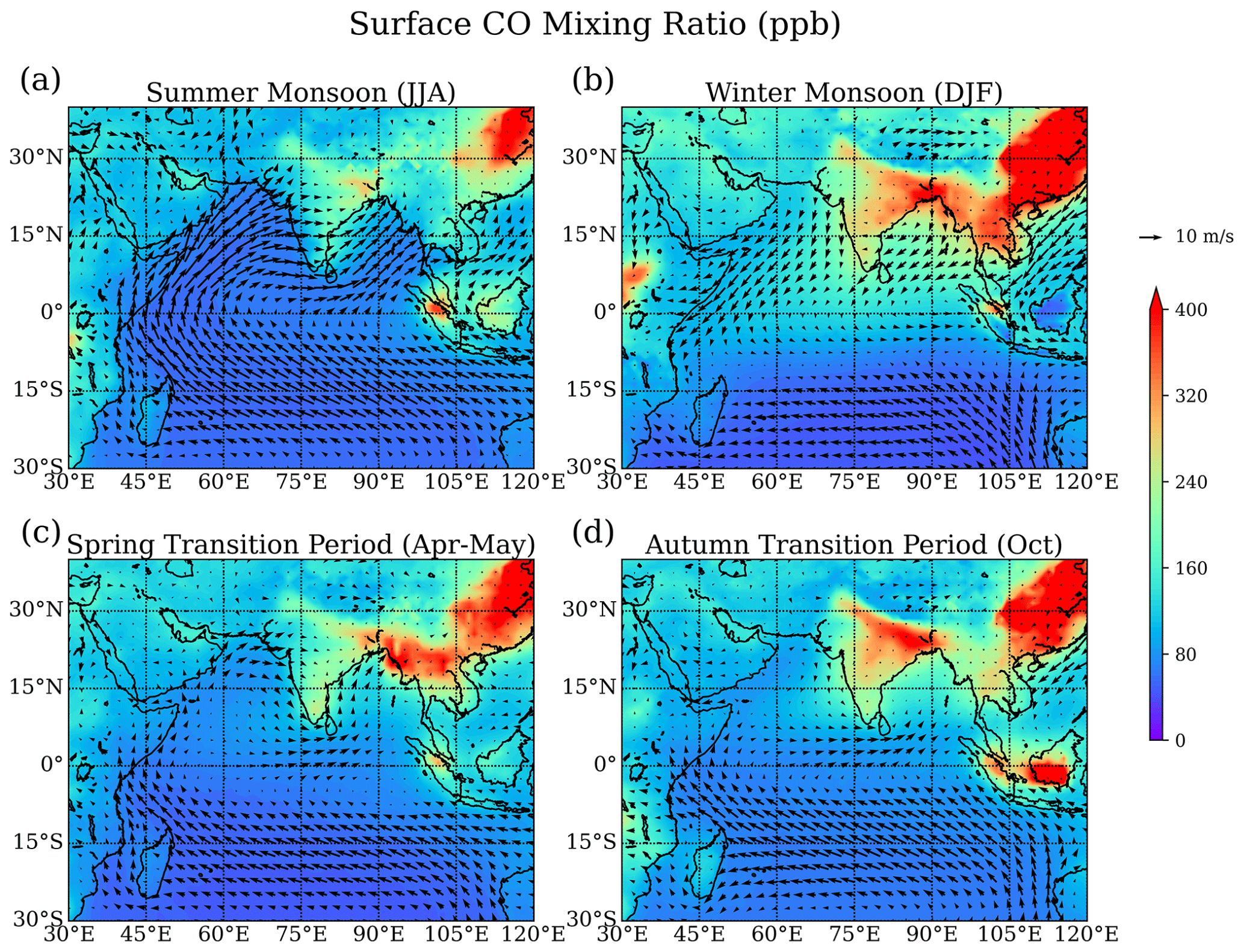
Figure 11 Surface carbon monoxide (CO) mixing ratios from MOPITT (colored shading) and surface wind from ERA-Interim (black arrows) for (a) summer monsoon 2014–2018 (June–August), (b) winter monsoon 2014/2015–2018/2019 (December–February), (c) spring transition 2014–2018 (April–May), and (d) autumn transition 2014–2018 (October).

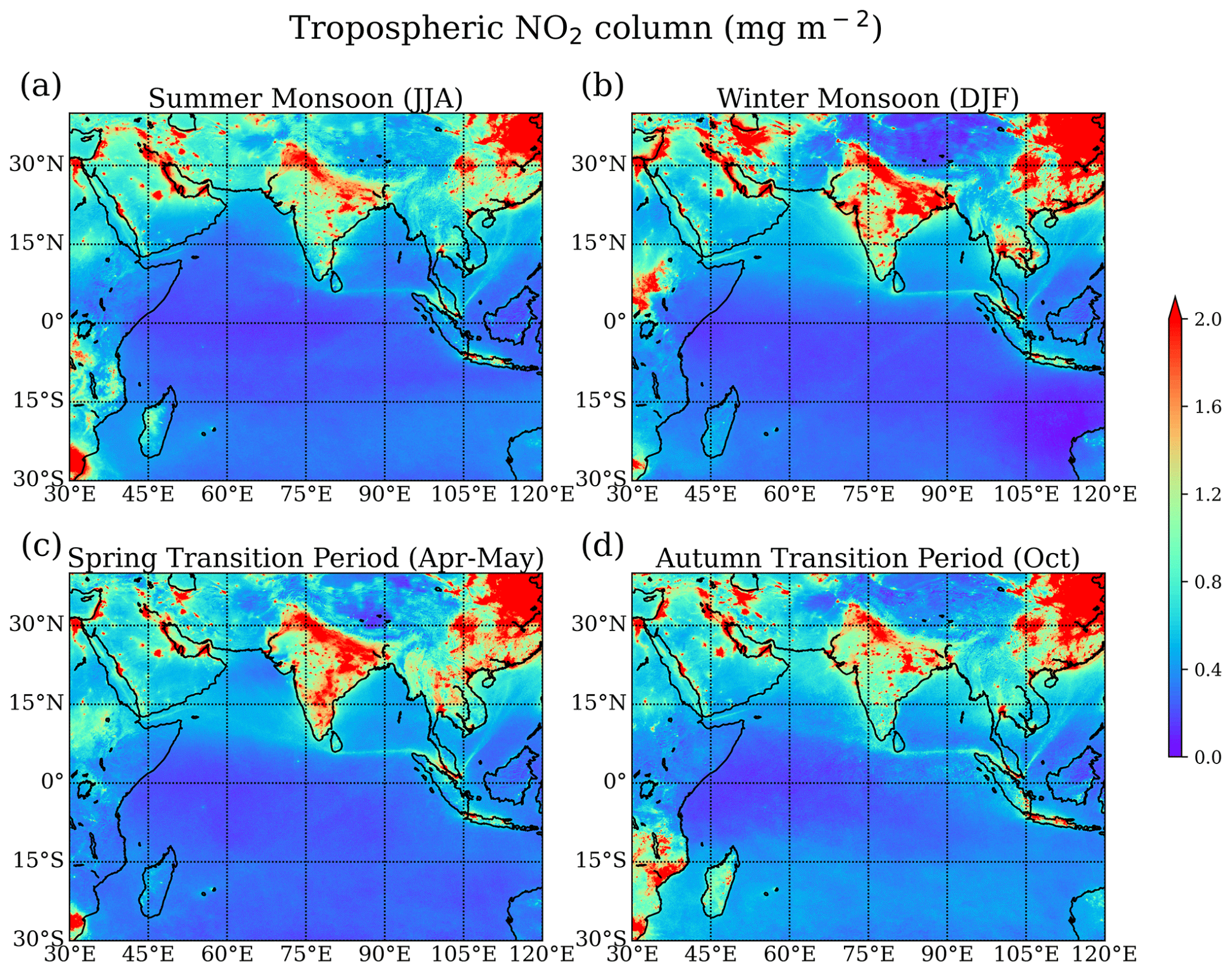
Figure 12 Tropospheric nitrogen dioxide (NO₂) column from TROPOMI for (a) summer monsoon 2019 (June–August), (b) winter monsoon 2018–2019 (December–February), (c) spring transition 2019 (April–May), and (d) autumn transition 2019 (October).

The tropospheric distribution of NO_x is relatively similar to that of CO but with larger variability on small scales and steeper gradients between the continental source regions and the Indian Ocean. Figure 12 shows the tropospheric NO₂ column from TROPOMI, which, due to the fast photochemical cycling between NO and NO₂, can be taken as a robust measure for concentrations of nitrogen oxides. Seasonal mean values for 2018–2019 show a clear gradient of NO₂, with maxima over the landmass source regions and minimum values over the equatorial western Indian Ocean (Fig. 12). Coastal gradients are particularly pronounced around the Indian coastline during the autumn transition period and winter monsoon. One clear difference in comparison to the CO distribution is the appearance of enhanced NO₂ columns along the shipping lanes, in particular along the major route at around 6^∘ N over the Bay of Bengal from the southern tip of India to Malaysia.

The INDOEX campaign showed that the winter monsoon season is characterized by strongly enhanced CO abundances over the northern Indian Ocean, with values comparable to air downwind of Europe and North America (Lawrence and Lelieveld, 2010). Based on simultaneous measurements of methyl cyanide (CH₃CN) and model simulations, biomass burning in South and Southeast Asia with subsequent transport of the polluted air towards the Indian Ocean was identified as a major source of CO (Lelieveld et al., 2001). Over the open Indian Ocean, southward transport along with chemical processing, dilution, and surface deposition cause a strong north–south pollution gradient. In the boundary layer, the contrast between polluted NH and pristine Southern Hemisphere (SH) air results in a sharp gradient across the ITCZ (Lawrence et al., 2003), while the upper troposphere was identified as a region for inter-hemispheric exchange of these air masses (Williams et al., 2002).

Recent studies of atmospheric composition during the winter monsoon period have focused on the Bay of Bengal where ship-based measurements were conducted during the second part of ICARB for December 2008–January 2009. Mixing ratios of NO₂ and CO show a distinct spatial pattern with elevated values in the head (northern part) and the southeastern Bay of Bengal due to transport from adjoining landmasses (Asatar and Nair, 2010; David et al., 2011). The in situ measurements reveal the highest CO surface mixing ratios of 379 ± 58 ppb over the southeastern Bay of Bengal, which exceed the MOPITT multi-annual mean values (Fig. 11b). Similar to CO, the NO₂ surface distribution exhibits prominent highs over the head and the southeastern Bay of Bengal, with lower values in the south (David et al., 2011). Analysis of back trajectories and airflow patterns revealed that the high pollution over the head of the Bay of Bengal (15–21^∘ N) was advected from the Indo-Gangetic Plain, which is one of the major CO emission centers (Fig. 2). The high pollution over the southeastern Bay of Bengal, on the other hand, was attributed to the effects of continental outflow from Southeast Asia, a transport pattern discernible from the wind patterns in Fig. 11. Airborne measurements conducted during the same campaign confirm the higher pollution over the northern and southeastern part of the Bay of Bengal (Srivastava et al., 2012b). Analyses of the acetylene $/$ CO ratio suggested that air mass samples taken over the northern Bay of Bengal were less chemically aged compared to samples taken during the other flights.

Enhanced wintertime CO values of up to 365 ppbv were also found in the Arabian Sea near the southwestern coast of India, while lower levels of around 50 ppb prevailed over the equatorial Indian Ocean during ICARB-2018 (Girach et al., 2020a). Consistent with previous campaign results, the authors linked the enhanced surface values to the impact of South Asian outflow. The study also highlighted the impact of convective outflow from Southeast Asia on the pollution levels. Enhanced CO in the upper troposphere (300–200 hPa) over the equatorial IO was suggested to result from anomalous westerlies associated with a disturbed Walker cell and the influence of African forest fires.

Seasonal variations of NO_x at a surface station in Trivandrum, situated on the southwestern coast of India, also show the highest values during the winter monsoon season due to land-based emissions and transport patterns (David and Nair, 2011). While the strongest NO_x emissions are located in East Asia, enhanced emissions also exist in southern India (Fig. 3), contributing to the wintertime NO_x maxima over the Indian coastline (see also Fig. 12). Ship-based observations of NO₂ show a strong decreasing gradient in concentrations from the subcontinent towards the open ocean. Observations made on the IIOE-2 expedition observed peak values of 854 ± 223 ppt close to Goa, but the values were below the detection limit of 120 ppt away from the coast. A similar gradient is evident from the satellite-retrieved tropospheric NO₂ with the emissions of NO_x over the subcontinent, leading to higher values close to the coast (Fig. 12; Mahajan et al., 2019a).

The impact of anthropogenic emissions during the winter monsoon is evident over large parts of the Indian Ocean, as demonstrated by surface measurements from the island of Mahé in the western Indian Ocean just south of the Equator. Seasonal variations of CO values peak in January–February as a result of the long-range transport of anthropogenic emissions from India during this time of year (Wai et al., 2014). Reunion Island around 19^∘ S, on the other hand, is much less impacted by the winter monsoon due to the ITCZ functioning as a transport barrier. Seasonal variations of CO measurements at two stations on Reunion Island peak in September–November, primarily driven by the emissions from biomass burning in Africa and South America (Zhou et al., 2018). The seasonal variations of the CO distribution given by the MOPITT satellite observations (Fig. 11) are consistent with the findings of the in situ measurement studies discussed above.

During the summer monsoon, CO mixing ratios over the Arabian Sea, Bay of Bengal, and Indian Ocean drop mostly below 80 ppb, except for over coastal waters in the Bay of Bengal with values of up to 150 ppb (Fig. 12). As the ITCZ moves north over the Indian subcontinent, the large-scale airflow is directed from the Indian Ocean towards the land, preventing the spread of pollution in the maritime environment. In addition, convective uplifting and mixing also contribute to lower CO abundances over the Bay of Bengal (Girach and Nair, 2014a). The coastal regions of Bangladesh and eastern India are exceptions, as they are impacted by strong westerlies transporting polluted air from southern India and Sri Lanka, resulting in elevated CO mixing ratios larger than 150 ppb (Fig. 11a). In situ measurements in 2018 conducted as part of IIOE-2 confirmed elevated CO levels up to 164 ppb downwind of Chennai, a coastal megacity in East India (Girach et al., 2020b). In addition, the impact of shipping emissions was detected near 6^∘ N with higher values of CO (up to 120 ppb) in the otherwise pristine air masses of the southern Bay of Bengal. The elevated pollution along the eastern Indian coastline is in stark contrast to the western Indian coastline, with very low CO mixing ratios of well below 100 ppb. The overall prevalence of clean oceanic background air during the summer monsoon season was confirmed by the low CO values detected over the equatorial Indian Ocean during the OMO campaign in July–August 2015 (Tomsche et al., 2019). Vertical profiles of CO were derived during flights over Gan (Maldives), which is situated close to the Equator and thus influenced by air from the southern Indian Ocean. The CO profiles over Gan, with values of ∼ 60 ppb, were found to be lower than the NH background and the Asian monsoon CO profiles for all altitudes below 8 km (Fig. 2 in Tomsche et al., 2019). During the AQABA ship campaign in summer 2017, low pollution levels over the Arabian Sea were confirmed by measurements of relatively low NO_x mixing ratios (0.19 ppb, Tadic et al., 2020).

The transition periods during boreal spring and autumn are characterized by large spatial and temporal variability of the pollution distribution, which shifts between the clean summer regime and the polluted winter regime. Mean CO mixing ratios in the Bay of Bengal and Arabian Sea range between 100 and 200 ppb, while the equatorial and southern Indian Ocean is dominated by clean oceanic air with CO values below 100 ppb (Fig. 12c and d). ICARB measurements during March–April 2006 show higher CO values in the Bay of Bengal compared to the Arabian Sea and higher CO values towards the coast, as expected with continental pollution being the main source of the observed values (Aneesh et al., 2008). Transport regimes start to shift in March when the outflow from India into the Arabian Sea and from Southeast Asia into the Bay of Bengal begins to weaken. This shift leads to slowly decreasing pollution, as observed during ICARB, with CO values over the northern Bay of Bengal found to be around 234 ppb during March (Srivastava et al., 2012a), thus being lower than the winter monsoon values discussed above. In April, offshore flow from the Indian subcontinent or Southeast Asia weakens further, leading to very little pollution transport towards the ocean. The southern Bay of Bengal is dominated by southwesterly winds (see also Fig. 12c) carrying cleaner marine air, as evident from CO mixing ratios of 88 ppb obtained during ICARB April measurements (Srivastava et al., 2012a).

The boreal autumn transition period, also referred to as the post-summer monsoon, marks the onset of the polluted winter regime after the withdrawal of the monsoon winds. During this period, a sudden increase in pollutant levels can be expected, in particular in coastal regions and over the Bay of Bengal. During the SK-277 ship campaign, large spatial heterogeneity of pollution was observed over the Bay of Bengal (Mallik et al., 2013), reflecting the direct impact of air masses being advected from different source regions in South Asia. The highest CO levels were found in air masses originating in Southeast Asia with signatures of biomass and biofuel burning. Continental pollution sources for NO_x were further enhanced by regional sources, possibly from ship emissions over the Bay of Bengal, which contains the international shipping corridor connecting the southern tip of India and the Strait of Malacca.

5.1.2 Sulfur dioxide (SO₂), mercury, and ammonia (NH₃)

In comparison to other pollutants, the SO₂ characterization above the Indian Ocean is sparse. Data available from the recent ICARB campaign in 2018, nonetheless, can be utilized to assess the influence of anthropogenic SO₂ in the marine atmosphere over the Indian Ocean by using non-sea-salt (nss) sulfate aerosol (SO${}_{\mathrm{4}}^{\mathrm{2}+}$) as a proxy for SO₂. Aswini et al. (2020) show the presence of nss-SO${}_{\mathrm{4}}^{\mathrm{2}+}$ in an intense pollution plume over the Arabian Sea and the Indian Ocean during the winter monsoon. Meteorological conditions during this season are favorable for SO₂ to nss-SO${}_{\mathrm{4}}^{\mathrm{2}+}$ conversion. This is proposed to take place through photochemical oxidation of SO₂ by the OH radical in the gas phase and through oxidation of SO₂ by H₂O₂ and O₃ in the aqueous phase (Seinfeld and Pandis, 2006). About two-thirds of the total tropospheric nss-SO${}_{\mathrm{4}}^{\mathrm{2}+}$ formation is thought to occur through aqueous-phase reactions (e.g., Warneck, 1999).

SO₂ has both anthropogenic and natural sources (i.e., oxidation of DMS), but comparison with previous research cruise studies conducted nearly 2 decades ago shows a more than twofold increase in the concentration of nss-sulfate aerosols over the continental outflow region in the Arabian Sea that appears to be due to anthropogenic SO₂ (Aswini et al., 2020). Despite decreasing SO₂ emissions in East Asia since 2010, emissions are rapidly increasing in South Asia, by about 10 % yr⁻¹, with the Indo-Gangetic Plain being a major source region (Lelieveld et al., 2019, Sect. 4). In order to further explore the contribution of anthropogenic SO₂ to nss-sulfate aerosol formation, the ratio of methanesulfonic acid (MSA), due solely to DMS oxidation, to nss-SO${}_{\mathrm{4}}^{\mathrm{2}+}$ was computed. The average MSA $/$ nss-SO${}_{\mathrm{4}}^{\mathrm{2}+}$ ratio during the ICARB campaign was 3.1 × 10³. Over the more pristine sections of the cruise, the average ratio was 4.7 × 10³. In remote marine regions, ratios of 0.065 have been found (Savoie and Prospero, 1989). The lower MSA $/$ nss-SO${}_{\mathrm{4}}^{\mathrm{2}+}$ ratio implies that most of the nss-SO${}_{\mathrm{4}}^{\mathrm{2}+}$ is from anthropogenic sources (Aswini et al., 2020).

Under the framework of the Global Mercury Observation System (GMOS) project, a mercury monitoring station was set up on Amsterdam Island, a remote and small island located in the southern Indian Ocean (Sprovieri et al., 2016). Observations of gaseous elemental mercury (GEM), reactive gaseous mercury (RGM), and particle-bound mercury (PBM) from this station over several years were reported by Angot et al. (2014). GEM concentrations were found to be remarkably steady, with an average hourly mean concentration of 1.03 ± 0.08 ng m⁻³, and show a small seasonal cycle. In comparison, the high-altitude GMOS site in Kodaikanal located in southern India shows significantly higher GEM concentrations of 1.54 ± 0.20 ng m⁻³ in 2013, possibly related to different long-range transport patterns and closer proximity of anthropogenic sources (Sprovieri et al., 2016).

RGM and PBM concentrations at Amsterdam Island were also very low (0.34 and 0.67 pg m⁻³, respectively) but displayed strong seasonal variability (ranging between the detection limit and 4.07 and 12.67 pg m⁻³, respectively). Analysis showed that, despite the remoteness of the island, long-range transport from southern Africa significantly contributed to the GEM and PBM budgets from July to September when biomass burning peaks in Africa (Angot et al., 2014). During these periods, the higher GEM concentrations observed at Amsterdam Island were comparable to those recorded at other tropical stations distributed around the globe. During periods of lower GEM concentrations, on the other hand, values of less than 1 ng m⁻³ were found to be characteristic for air masses from the southern Indian Ocean and Antarctic continent (Sprovieri et al., 2016).

Observations of ambient ammonia (NH₃) are rare in the Indian Ocean region. Recent measurements of NH₄ in aerosols over the Indian Ocean have been related to gaseous NH₃ emissions from land (either anthropogenic or crustal sources, Aryasree et al., 2015; Aswini et al., 2020). Earlier direct observations in 1980 by Ayers and Gras (1980) in the southern Indian Ocean showed a range between 2.2 and 4.4 nmol m⁻³. Later observations in the same region of the ocean showed a lower range of 0.3 to 2.1 nmol m⁻³ (mean of 1.1 nmol m⁻³) (Norman and Leck, 2005). In the northwestern Arabian Sea, observations of NH₃ were first carried out in 1999, reporting higher concentrations in the coastal environment of 2.5 to 5.6 nmol m⁻³ (mean 3.8 nmol m⁻³) compared to the remote open-ocean environment of 0.4 to 1.8 nmol m⁻³ (mean 1 nmol m⁻³), showing the importance of continental fluxes for the ambient marine NH₃ loading (Gibb et al., 1999). Similar to the southern Indian Ocean, later observations by Norman and Leck (2005) again reported a lower range between 0.05 and 0.2 nmol m⁻³ (0.1 nmol m⁻³). The reason for this discrepancy between the two studies is not clear and was not discussed in the study by Norman and Leck (2005).

Closer to the Indian coast, observations of NH₃ have been made in the Bay of Bengal over five studies and show much higher concentrations compared to the central or southern Indian Ocean. Khemani et al. (1987) reported high concentrations of NH₃ in the coastal region in the range between 117.6 and 211.8 nmol m⁻³ (mean 158.8 nmol m⁻³). Later, Carmichael et al. (2003) also reported high NH₃ concentrations at two coastal sites (Bhubneswar: mean 288.2 nmol m⁻³, Berhampur: mean 329.4 nmol m⁻³). These observations show a west–east positive gradient close to the western coast of the Bay of Bengal, which is most likely driven by the local transport of NH₃. Further to the northwest, Biswas et al. (2005) made observations of ambient NH₃ close to the Sundarban mangrove forest, which is one of the largest river deltas in the world. They saw highly elevated levels ranging from 105.2 to 675.0 nmol m⁻³ (mean 265.2 nmol m⁻³). The most recent reports in the literature were measurements done during the winter phase of ICARB in the Bay of Bengal, which reported an average concentration ranging between 11.7 and 441.2 nmol m⁻³ (mean 281.2 nmol m⁻³), with higher concentrations observed closer to the coast and lower concentrations observed in the open-ocean environment (Sharma et al., 2012). Unfortunately, no seasonal information is available due to the lack of continuous observations through the entire year in the marine environment.

5.1.3 Ozone

Ozone distribution over the Indian Ocean is largely determined by the abundance of precursor gases, transport patterns, and chemical processing. During the winter monsoon, the southern Asian outflow brings ozone precursors such as CO, NO_x, and VOCs from their source regions in South and East Asia (Sect. 4) into the marine environment. Within the outflow, substantial photochemical production of ozone occurs due to high pollution levels and strong tropical solar radiation, which is particularly effective under cloud-free conditions. As a result, relatively high ozone mixing ratios of 60–70 ppb have been observed off the coast of India and over the Bay of Bengal up to a few hundred kilometers downwind (Lawrence and Lelieveld, 2010, and references therein). Similarly, high concentrations of up to 80 ppb have also been reported off the western Indian coast in the Arabian Sea (Lal and Lawrence, 2001). Once produced, ozone can be transported to the remote marine environment, where local dominant sources of ozone precursor gases are absent. As a result, the marine boundary layer is considered an ideal place to study the processes that drive ozone photochemistry (e.g., Monks et al., 1998). Tropospheric ozone is also influenced by downward transport from the stratosphere (e.g., Ganguly and Tzanis, 2011) and deposition to surfaces (Graedel and Crutzen, 1992). Photo-dissociation of ozone leads to increasing OH levels, particularly within the highly humid marine boundary layer, affecting the chemistry of the tropical marine environment and highlighting the importance of continental outflow over cleaner oceanic regions.

A continuous dataset of ozone vertical profiles at Ahmedabad, a city in western India, shows a clear annual cycle dominated by transport patterns (Lal et al., 2014). The lowest ozone (∼ 20 ppb) was observed near the surface during September, which is at the end of the summer monsoon. Clean air from the ocean and removal of precursors due to monsoon rains drive this reduction. Model simulations showed that the lower-tropospheric (< 3 km) ozone during the summer monsoon was transported from the Indian Ocean via the east coast of Africa and the Arabian Sea. Observations of mid-tropospheric ozone are highest (70–75 ppb) during April–June and lowest (40–50 ppb) during winter due to the impact of long-range transport from North Africa, North America, and the stratosphere. Balloon-borne ozone measurements during 2011–2014 at the southwest coast of India confirmed the highly dynamic nature of tropospheric ozone profiles (Ajayakumar et al., 2019). The variations in their vertical structure and short-term changes can be attributed to photochemistry as well as meteorological conditions in the form of synoptic-scale systems, long-range transport, and stratospheric intrusions. Unfortunately, such continuous measurements are not available at any site off the Indian subcontinent, but model simulations suggest that a similar annual cycle can also be expected in the northern Indian Ocean environment (Lal et al., 2014).

During the winter monsoon, measurements of ozone in the Bay of Bengal were carried out as a part of the ICARB campaign (David et al., 2011). The marine boundary layer showed large variations in the mixing ratios of ozone and its precursor gases with similar spatial patterns (Fig. 13a), pointing to the same source regions but different relative contributions. In the head and southeast of the Bay of Bengal, mixing ratios of ozone (61 ± 7 and 53 ± 6 ppb) and precursors (discussed earlier) were found to be very high. Air mass back trajectories originated from the Indo-Gangetic Plain and Southeast Asian countries, respectively, and both are characterized by high tropospheric ozone and NO₂ values. In the south and southwestern part of the Bay of Bengal, the ozone mixing ratios were low, and the back trajectories originated from coastal regions. Here, the longer transit times over the marine environment could have resulted in the OH-driven destruction of ozone and precursors as well as in changes in surface-level mixing ratios due to updrafts and downdrafts (David et al., 2011). Over this oceanic region, photochemical production involving NO₂ did not play a major role in ozone production, while the high water vapor acted as a sink.

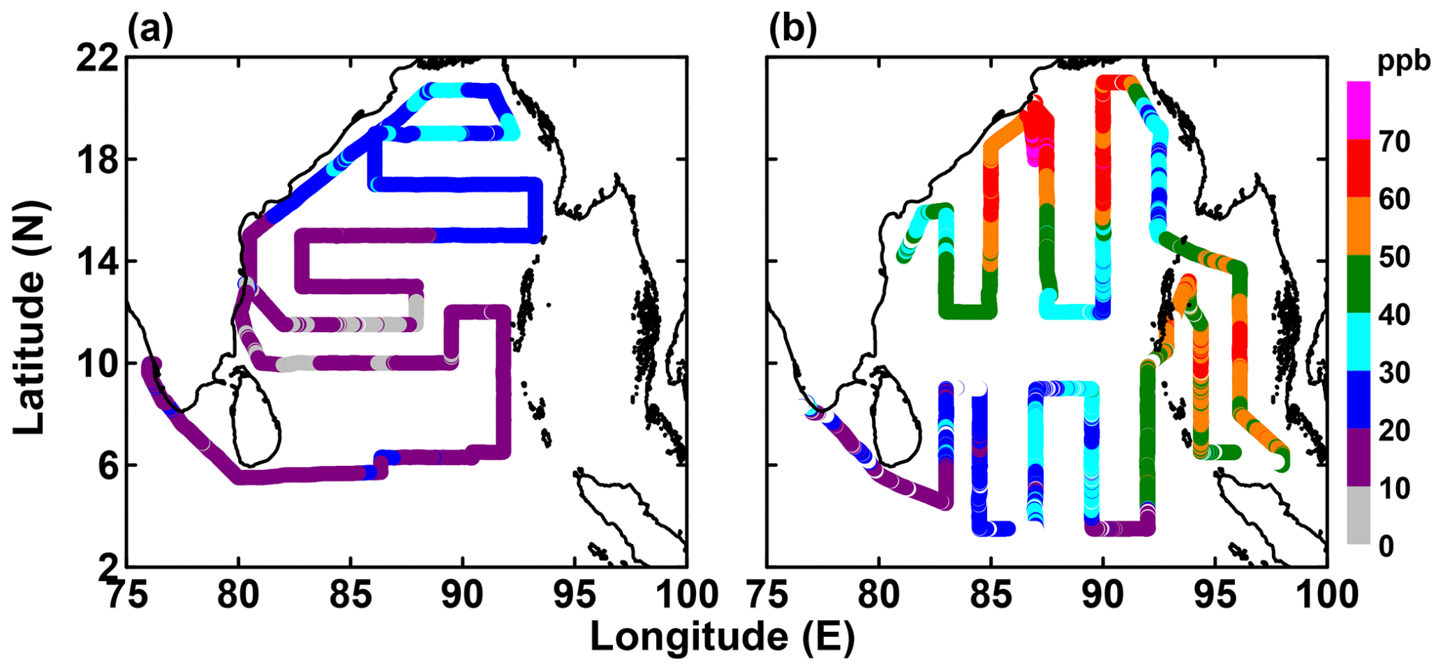
Figure 13 Surface ozone mixing ratios in the Bay of Bengal observed during (a) boreal spring (March–April 2006, ICARB) and (b) winter monsoon (December–January 2009, ICARB). From David et al. (2011), © 2011; reproduced with permission.

Observations during the spring transition season of near-surface ozone in the Bay of Bengal were carried out as part of the first ICARB phase during March and April 2006 (Fig. 13b). Over the northern Bay of Bengal, higher ozone mixing ratios (∼ 30 ppb, Nair et al., 2011) were found to be well correlated with precursor gases, indicating their co-located sources (Srivastava et al., 2012a). Similar to the winter monsoon conditions, northwesterly winds transported large quantities of anthropogenic pollutants from the Indo-Gangetic Plain to the northern part of the Bay of Bengal, causing the elevated pollution levels. The middle and southern Bay of Bengal was more influenced by the open-ocean environment and showed lower ozone mixing ratios (∼ 10–15 ppb, Nair et al., 2011). For both regions, the surface ozone mixing ratios were anticorrelated with the boundary layer height. Ozonesonde measurements taken during the same campaign revealed an elevated plume between 1 and 3 km over the northern Bay of Bengal with very high ozone mixing ratios of 60–90 ppb (Srivastava et al., 2011; Lal et al., 2013). The plume was also characterized by higher temperature and lower specific humidity compared to the background marine air over other regions. This elevated layer sandwiched between the marine boundary layer and the free troposphere can be attributed to the advection of land air mass as a consequence of land–sea breeze circulation near the coast or long-range transport. Ozone profiles in the first 3 km over the Arabian Sea are around 10 ppb lower than over the Bay of Bengal (Lal et al., 2013). Above this height, ozone levels are about 20 ppb higher over the Arabian Sea, possibly due to intrusions of ozone-rich air from upper levels.

Observations over the Arabian Sea during the spring transition period revealed a completely different picture. Ozone and pollutants showed significantly lower mixing ratios when compared to the northern Bay of Bengal, suggesting a larger impact of cleaner marine air (Srivastava et al., 2012a). This argument is further supported by the poor inter-correlations of ozone and the various precursors. Based on simulations with the Model for OZone And Related Tracers (MOZART), a global chemical transport model, the authors hypothesize that loss of ozone due to halogen chemistry might be an additional reason for the relatively low ozone abundances over the Arabian Sea. Latitudinal gradients of the gases were slightly negative, most likely due to some transport of polluted air from southern India over the southern Arabian Sea and continuous dilution of pollution with time over this region. Such negative pollution gradients over the Arabian Sea during the transition periods were confirmed by the CO distribution obtained from MOPITT (Srivastava et al., 2012a; Fig. 11c and d).

During the summer monsoon period, unusually low levels of ozone (9 ppb) were reported for the Arabian Sea during the ARMEX campaign in 2002 (Ali et al., 2009). Based on MOZART model simulations, the authors attribute the low ozone abundances to chemical loss driven by reactive halogens from sea salt, which can account for up to 30 % of the total ozone loss (2.15 ppb d⁻¹). In addition, increased marine surface reactivity facilitated enhanced dry deposition of ozone (∼ 0.12 ppb d⁻¹) and thus also contributed to the observed low ozone levels. Summer monsoon ozone measurements close to the Arabian Peninsula are available from the AQABA ship campaign in 2017. Consistent with the low pollution levels detected in this region, ozone mixing ratios were relatively low (22.5 ppb), representing remote MBL conditions (Tadic et al., 2020). Net ozone production rates did not significantly deviate from zero and indicate weak net ozone production of 5 ppb d⁻¹. In contrast, measurements during the rest of the campaign in the Red Sea, Gulf of Oman, and Arabian Gulf revealed strongly enhanced tropospheric ozone with larger ozone production rates of up to 28 ppb d⁻¹. The sensitivity of ozone production to the prevailing conditions was assessed by defining ozone production regimes in terms of the OH reactivities of VOCs and NO_x. Based on this analysis, the relatively clean air of the Arabian Sea was found to be due to partially NO_x-limited ozone production in this region (Pfannerstill et al., 2019).

Summer monsoon measurements in the Bay of Bengal report enhanced ozone and pollution levels over the coastal regions, in particular downwind of the tropical megacity Chennai. The Copernicus Atmosphere Monitoring Service (CAMS) model simulations suggest that in the Chennai plume, VOC-limited ozone production dominates in the morning and gradually shifts to a NO_x-limited regime in the afternoon (Girach et al., 2020b).

During the autumn transition season, simultaneous measurements of ozone and precursors were made over the Bay of Bengal in October–November 2010. These measurements revealed large variability in ozone (11–60 ppb) with maximum values found in the northern Bay of Bengal. Back trajectory analysis led to a similar conclusion as the abovementioned ICARB study, revealing the influence of pollution plumes from the India–Bangladesh region and Southeast Asia in addition to long-range transport of pristine marine air from the Indian Ocean (Mallik et al., 2013). Diurnal variations found in surface ozone were also attributed to the interplay of these two processes.

In addition to the studies focusing on the Bay of Bengal and the Arabian Sea, observations of ozone were made along two ship tracks from the east and west of the Indian subcontinent, respectively, heading towards the open oceans during December–March as a part of ISOE 8 (2014) and IIOE-2 (2015). The ISOE 8 campaign started from Chennai on the east coast and headed towards the Southern Ocean, while IIOE-2 started in Goa and went across the Arabian Sea and the northern equatorial Indian Ocean towards Mauritius. Both campaigns show a strong reduction in the ozone concentrations from ∼ 50 to ∼ 5–10 ppb within a few degrees off the Indian coast (Mahajan et al., 2019a, b), demonstrating that continental emissions are the main drivers behind the high ozone concentrations close to the Indian subcontinent.

Diurnal variations of ozone in the marine boundary layer are driven by effects of large-scale horizontal advection from source regions, entrainment of ozone-rich air from higher altitudes, photochemical production involving precursor gases, and loss mechanisms involving OH radicals. Over the last decade, significant progress has been made in understanding how the different processes determine diurnal ozone variations based on in situ observations corroborated by chemistry simulations from box models, regional forecast models, and chemical reanalysis.

In polluted air masses, daytime photochemical production of ozone from anthropogenic precursors such as NO_x has been observed (Nair et al., 2011; Mallik et al., 2013; Girach et al., 2020b). Such photochemical production only occurs if a sufficient amount of precursor gas is present and leads to peak ozone values around noon. Ozone daytime build-up has been identified downwind of the shipping lane over the Bay of Bengal (Girach et al., 2020b) and close to coastal cities (Nair et al., 2011).

In pristine air masses over the Indian Ocean with low pollution levels and high water vapor, photochemical destruction of surface ozone occurs during daytime (Nair et al., 2011; Mallik et al., 2013; Girach et al., 2020b). Photolysis of ozone produces O(¹D), which reacts with H₂O and produces OH radicals, with the latter causing the destruction of ozone (Pitts and Pitts, 2000). An increase in the absolute water vapor content was found to coincide with the decrease in ozone and vice versa (Nair et al., 2011). During the nighttime, ozone-rich air can be entrained from the free troposphere into the marine boundary layer, allowing ozone recovery and leading to next-day daytime destruction. Box model simulations have highlighted the importance of such entrainment processes given their high sensitivity to various background levels of ozone (Mallik et al., 2013).

In the remote marine regions, ozone is known to show “virtually no diurnal variation” (Liu et al., 1983) due to the scarcity of precursor gases and the lack of exchange between the ozone-rich free troposphere and the ozone-poor boundary layer. The absence of in situ photochemical production of ozone has been observed during various Indian Ocean campaigns (e.g., Sahu et al., 2006; Lal et al., 2007; Girach et al., 2017, 2018). Such absence of daytime ozone build-up suggests that the observed spatiotemporal variations in surface ozone can be attributed to in situ photochemical build-up in air masses moving from coastal polluted regions towards the Indian Ocean (Ojha et al., 2012; Girach et al., 2018). Ozone simulations with the Weather Research and Forecasting model with Chemistry (WRF-Chem) along air mass trajectories suggest mean en route ozone production in the outflow towards the Bay of Bengal (Girach et al., 2017).

Table 4 Ozone (O₃) mean values (ppb) and latitudinal gradients reported for various campaigns in the Bay of Bengal, Arabian Sea, and Indian Ocean. Ozone maximum values are given in the marine boundary layer (MBL) and in the elevated layer (EL), as available.

Available ozone measurements from campaigns conducted in the Bay of Bengal, Arabian Sea, and Indian Ocean over the last decades have been summarized in Table 4. The measurements reveal some clear spatial and seasonal patterns, with the highest ozone mixing ratios during the winter monsoon, in particular in the Bay of Bengal and Arabian Sea. On average, ozone abundances decrease during the spring transition period and increase again after the summer monsoon. Nearly all campaigns detected the highest ozone values close to the northern continental landmasses, reflecting the direct impact of air masses originating from different pollution source regions in South Asia and the Indo-Gangetic Plain. However, the situation can also be reversed, with higher levels of ozone observed over the central Bay of Bengal, not near the coastal regions (Lal et al., 2006), due to different types of wind patterns and possible titration by fresh emissions of NO. Sharp latitudinal gradients ranging from 1.3 to 5.4 ppb O₃ per degree with increasing ozone towards northern landmasses were identified during all campaigns except for ICARB measurements in the Arabian Sea during the spring transition period. The strength of the gradients depends on the season, with sharper gradients during the winter and sometimes transition periods, as well as on the latitudinal extent, with sharper gradients closer to the coastlines. Land–sea-breeze-triggered transport of polluted air masses in the elevated layer can lead to substantially higher ozone values above the MBL, as demonstrated during the campaigns in which ozonesonde measurements were available. Direct comparisons of ozone values in the Bay of Bengal and the Arabian Sea are in most cases not possible, except for the ICARB spring campaign during which ozone peaked in the Bay of Bengal.

5.2 Greenhouse gases

Greenhouse gases are largely emitted from anthropogenic activities over the continents, as are most of the atmospheric pollutants discussed above (Sect. 4). Therefore, greenhouse gases and pollution show a similar spatial distribution with higher values towards the coast and lower values over the open ocean. However, greenhouse gases have generally longer lifetimes, resulting in overall smaller spatial gradients. In addition, they often have large sources from the terrestrial biosphere of the NH midlatitudes, which can impact their seasonal cycle over coastal and open-ocean regions. In the following section, we discuss the distribution and variability of the greenhouse gases CH₄, N₂O, CO₂, and COS.

5.2.1 Methane (CH₄)

In situ observations collected over the last 2 decades have significantly contributed to our current understanding of the large-scale CH₄ distribution. During the summer monsoon season, near-surface CH₄ mixing ratios of 1830 ± 140 ppb were detected over the northern Bay of Bengal during the 2009 CTCZ campaign (Girach et al., 2017). Back trajectory simulations linked the enhanced values over the Bay of Bengal to emissions from central and northern India. Ship data collected during the winter monsoon show decreasing CH₄ mixing ratios from the northern (1910 ppb) to southern Bay of Bengal (1750 ppb) and slightly smaller abundances over the Arabian Sea (1700 to 1800 ppb) (Srivastava et al., 2012a). Station data for 1993–2002 from the west coast of India revealed large seasonal variations with maximum values of up to 1980 ppb at the beginning of the winter monsoon season (Bhattacharya et al., 2009) related to the interplay of seasonal variations in emissions and transport. CH₄ production from Asian rice cultivation maximizes during the autumn transition season when the plants are fully grown (Sect. 4.2). At the same time, the onset of the winter regime starts to allow for air mass transport from continental regions with significant anthropogenic influence. During the winter monsoon, these transport patterns intensify, bringing air masses with elevated CH₄ over the Indian Ocean.

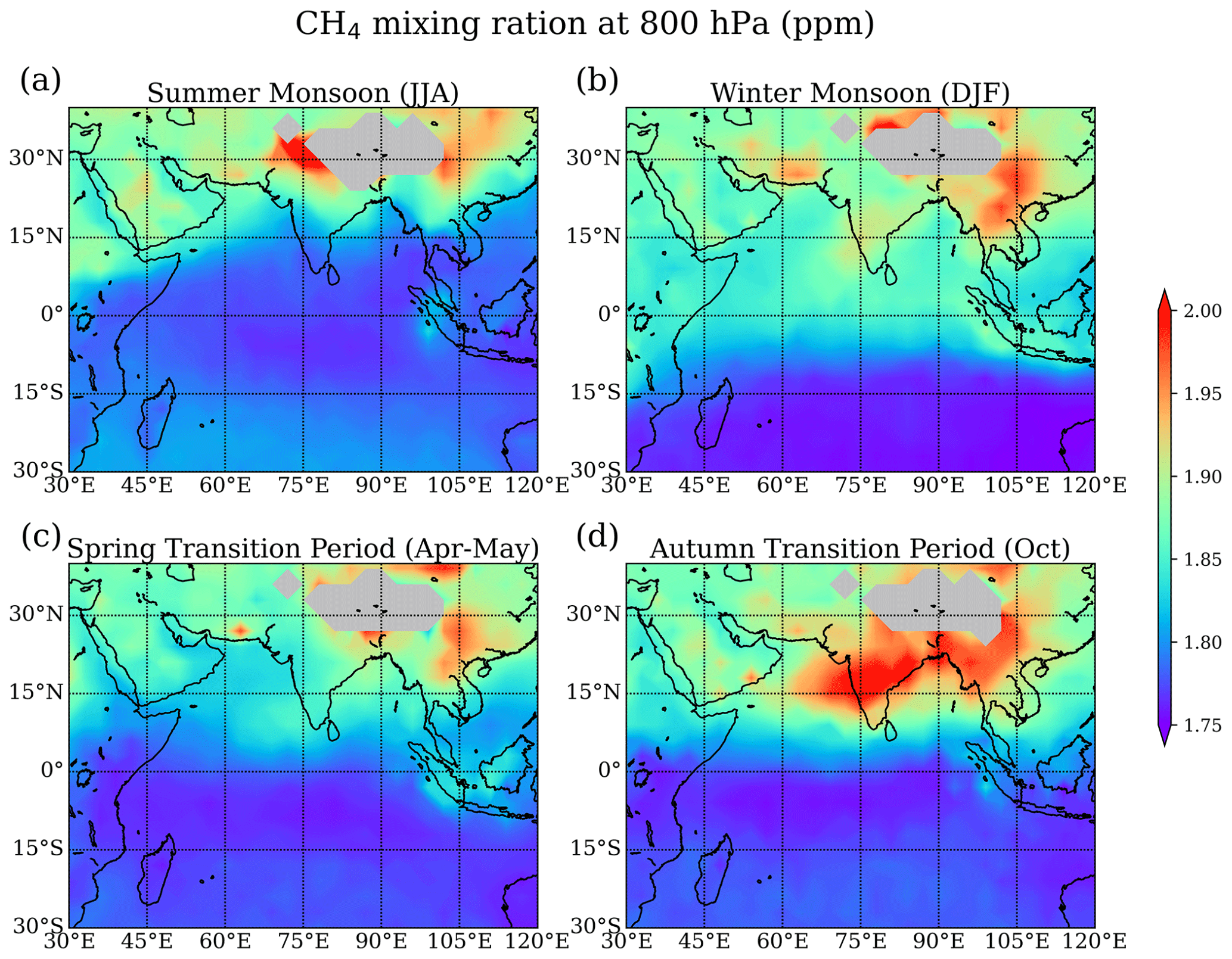
Figure 14 Methane (CH₄) mixing ratios at 800 hPa from GOSAT for (a) summer monsoon 2009–2014 (June–August), (b) winter monsoon 2009/2010–2014/2015 (December–February), (c) spring transition 2009–2014 (April–May), and (d) autumn transition 2009–2004 (October).

The three-dimensional distribution of CH₄ above the boundary layer over the Arabian Sea, Bay of Bengal, and Indian Ocean can be investigated based on GOSAT satellite measurements (Fig. 14; CH₄ at 800 hPa). CH₄ is higher towards the coast and lower over the open ocean due to the proximity of source-rich land regions. In particular, the fossil fuel mining areas in the Arab region are believed to contribute to enhanced CH₄ over the northern Arabian Sea (Kavitha and Nair, 2019). Overall, latitudinal CH₄ variations between 20^∘ N and 30^∘ S of up to 6 % are much smaller than latitudinal variations of CO over the same region of up to 150 %. Consistent with in situ surface measurements, CH₄ at the top of the boundary layer of the eastern Arabian Sea and Bay of Bengal maximizes during the autumn transition and winter monsoon seasons. Peak values of over 2000 ppb appear over the northern Bay of Bengal and along the Indian west coast. The overall spatial distribution does not change much with height, and at all altitudes between 850 and 200 hPa the highest CH₄ values are found over the northern Arabian Sea and northern Bay of Bengal (Kavitha and Nair, 2019). Similarly, the monthly variations of CH₄ mixing ratios over all oceanic regions remain more or less similar at all altitudes, with a peak during the autumn transition season.

Over the equatorial Indian Ocean, CH₄ values at the top of boundary layer are relatively low during all seasons, with values mostly below 1800 ppb, except for the winter season during which values can reach 1870 ppb (Fig. 14b). The OMO aircraft campaign in July–August 2015 confirmed low CH₄ values detected by the satellite for the summer monsoon. Observations over Gan (Maldives) show average CH₄ mixing ratios of 1778.3 ± 19.5 ppb during the summer period, being significantly lower than in the NH background or the Asian monsoon profiles (Tomsche et al., 2019). CH₄ mixing ratios increase with height due to inter-hemispheric transport mixing NH air masses into the SH at higher altitudes. As the NH air masses have experienced convective uplift from the boundary layer, they advect higher CH₄ mixing ratios into the SH (Bergamaschi et al., 2013).

The SH Indian Ocean has been found to be much less impacted by the winter monsoon compared to the NH Indian Ocean due to the ITCZ functioning as a transport barrier. In situ measurements from Reunion Island around 19^∘ S suggest the opposite seasonal cycle, with the lowest CH₄ values in December–February and highest CH₄ values in August–September (Zhou et al., 2018). Here, the CH₄ seasonal variability is not dominated by nearby land sources, but rather by seasonal variations of OH radicals.

5.2.2 Nitrous oxide (N₂O)

Measurements of N₂O over the Indian Ocean are sparse. The distribution of N₂O derived during a ship campaign in the Arabian Sea, equatorial Indian Ocean, and southwest part of the Bay of Bengal during the autumn transition period (October–November 2004) reveals clear latitudinal gradients (Mandal et al., 2006). Near the coast, N₂O values of 312 ppb were found, and they increased towards the open ocean, with a maximum of 432 ppb at the Equator. In the equatorial SH, N₂O decreased sharply to 312 ppb and did not change substantially during the rest of the cruise along the Equator and in the southwest part of the Bay of Bengal. Given the sparse data it is difficult to determine if the peak values around the Equator are caused by local oceanic emissions or are related to long-range transport from other sources.

5.2.3 Carbon dioxide (CO₂)

CO₂ satellite-based observations over the Indian Ocean reveal strong seasonal and latitudinal gradients (Nalini et al., 2018; Nayak et al., 2011). During most seasons, larger CO₂ values over the southern and southeastern Asian landmasses are accompanied by pronounced latitudinal gradients over the coastal regions and lower CO₂ values over the ocean. This distribution has been confirmed by ship-based observations during the summer monsoon (Kumar et al., 2014) and autumn transition season (Mandal et al., 2006). The measurements showed elevated CO₂ with large variability near the coastal region and relatively low CO₂ with correspondingly lower variability over the open ocean.

CO₂ over the Bay of Bengal and Arabian Sea is characterized by a pronounced seasonal cycle, with the highest values in boreal spring and lowest values in autumn (Nalini et al., 2018). Satellite observations show that during winter, a band of relatively low CO₂ mixing ratios (376–378 ppm) extends over the northern Indian Ocean at 0–25^∘ N in the west–east direction, where the smallest values exist over the western Arabian Sea (Nayak et al., 2011). During boreal spring, the CO₂ in this region increases, in particular over the Bay of Bengal. Seasonality over the southern Indian Ocean shows a different pattern. Similarly to the northern part, a belt of low CO₂ is found during boreal winter between 10 and 25^∘ S. During boreal spring, however, this band of relatively low CO₂ values remains prominent (Nayak et al., 2011), highlighting the potential role of this region as an oceanic CO₂ sink (Sect. 4.2). In addition, Valsala et al. (2020) used 60 years of reanalysis data to determine that atmospheric mixing ratios over the southeastern tropical region are driven by the Indian Ocean Dipole.

Lagrangian transport simulations, carried out to analyze the seasonal cycle at two Indian coastal stations, suggest that the seasonality of the CO₂ distribution over the Indian Ocean is driven by atmospheric circulation changes combined with the seasonal cycle of CO₂ over land regions (Nalini et al., 2018). While dominant marine contributions during the summer monsoon result in slowly decaying values, the winter and spring monsoon season is characterized by sources from the eastern continental landmasses, leading to maximum values over the coastal stations during spring. The equatorial Indian Ocean, on the other hand, shows only a weak seasonal cycle when compared to Indian coastal locations, the Bay of Bengal, and the Arabian Sea. Here, contributions from oceanic regions dominate during all seasons, with smaller continental contributions during the winter period. Overall, the anthropogenic emissions over the continental landmasses appear not to be a large source for CO₂ in the open Indian Ocean environment.

5.2.4 Carbonyl sulfide (COS)

There are only three published datasets of ship- or land-based observations of COS mixing ratios over the Indian Ocean. The measurements were made over the course of a year at Amsterdam Island (Mihalopoulos et al., 1991), on a research cruise in the eastern and southern Indian Ocean in November (Inomata et al., 2006), and on the OASIS research cruise in the western tropical Indian Ocean in July (Lennartz et al., 2017, see Sect. 3). All measured COS values are either at or below the global mean COS atmospheric mixing ratio of 549 ppt and exhibit no clear seasonal or latitudinal pattern (Lennartz et al., 2020). Satellite measurements and inverse modeling studies show elevated values of the atmospheric COS mixing ratio over the Indian Ocean, but the values are not as high as those over the Pacific Ocean and Maritime Continent at similar latitudes (Glatthor et al., 2015; Kuai et al., 2015). The elevated values have led to the hypothesis that the northern Indian Ocean is one of the missing source regions (Kuai et al., 2015). Given the lack of compelling evidence from surface ocean measurements, however, it does not appear that the Indian Ocean is the location of the missing source. Instead, anthropogenic sources around Southeast Asia could be responsible, as discussed in Sect. 4.

5.3 VOCs and short-lived gases DMS, isoprene, and halogens

5.3.1 VOCs

The VOC mixing ratios over the Bay of Bengal are higher during the winter monsoon than during the summer monsoon for most VOCs, but with clear north–south gradients all year-round (Sahu et al., 2011). Alkenes show an opposite seasonality to the rest of the major VOCs, with higher mixing ratios during the summer monsoon and no clear latitudinal gradients. For the other major VOCs, latitudinal gradients during the summer monsoon are caused by the transport of pollutants from peninsular India to the northern Bay of Bengal and clean marine air over the southern Bay of Bengal. Latitudinal gradients during the winter monsoon are ascribed to dilution and increased photochemical loss towards the southern Bay of Bengal. However, measurements along the coasts during both seasons showed no clear latitudinal trend and were influenced by photochemistry and stagnant airflow. Seasonal changes in the distribution of VOCs in the surface layer over the Bay of Bengal resemble changes in wind speed (Sahu et al., 2010). Diurnal variability of alkenes is evident in summer but not winter, and there is evidence that cyclones and convective activities in the summer season impact their mixing ratios. High mixing ratios are also found over the Arabian Gulf (Bourtsoukidis et al., 2020). VOC measurements at the Maïdo observatory in the southern Indian Ocean over 2 years reveal VOCs in the surface layer from anthropogenic sources (38 %), biomass burning (33 %), and both primary (15 %) and secondary (14 %) biogenic sources (Verreyken et al., 2021).

Regarding HCHO, Gopikrishnan and Kuttippurath (2021) used satellite measurements for the period 2005–2014 and found large amounts along the ship routes in the Indian Ocean. The values were double the natural background without the presence of ships. The trend in HCHO concentrations over the Indian Ocean shipping lanes is about 0.008 × 10¹⁵ molecules cm⁻² yr⁻¹. In general, the HCHO values and trends from the northern Indian Ocean routes are comparable to those in the Panama Canal, Mediterranean Sea, and Strait of Malacca.

5.3.2 DMS and isoprene

DMS in the Arabian Sea is projected to act as a relatively large oceanic source of sulfur to the atmosphere during the Asian summer monsoon season (Lana et al., 2011). These high emissions have been confirmed by recent ship-based measurements during the AQABA campaign, identifying elevated DMS values in the atmosphere ranging from 100 to 500 ppt (Edtbauer et al., 2020). Given the low atmospheric background pollution and the elevated DMS mixing ratios, the latter was found among the 10 most important OH sinks with a reactivity of 0.02 s⁻¹ (Pfannerstill et al., 2019). During the OASIS campaign, similar atmospheric mixing ratios of approximately 20–300 ppt were measured over the western tropical Indian Ocean. The atmospheric distribution patterns in time and space during OASIS generally matched measured fluxes (Zavarsky et al., 2018b). During this study, the directly measured DMS fluxes, as well as calculated isoprene fluxes and sea spray fluxes, were correlated with satellite-derived aerosol products over the region. Many of the correlations, which took into account the influence of regional transport based on air mass trajectories, were statistically significant. The aerosol product distribution more closely resembled the trace gas fluxes than the sea spray flux distributions. Thus, sea spray appears to be more of a minor precursor than the trace gases. This is supported by Quinn et al. (2017), who found a 30 % contribution of sea spray to cloud condensation nuclei in the tropics. These results illustrate the importance of the regional coupling between marine-derived gaseous precursors and aerosol products in the remote MBL, which can give rise to local feedback processes (Zavarsky et al., 2018b).

The longest continuous observations of atmospheric DMS in the Indian Ocean were obtained at Amsterdam Island (37.8^∘ S, 77.5^∘ E) in the southern Indian Ocean (Scaire et al., 2000). Measurements from 1990 to 1999 revealed atmospheric DMS ranging from 5 to 1900 ppt with a clear seasonal cycle. Maximum DMS values in January were on average 20 times higher than minimum values in July–August. These strong seasonal variations are not caused by atmospheric transport patterns but are linked to a similar cycle in DMS concentration in seawater induced by enhanced phytoplanktonic activity during the boreal summer. Model runs using the Lana et al. (2011) climatology show a good match with these observations, confirming the dominant impact of oceanic processes on atmospheric DMS concentrations over the open Indian Ocean (Mahajan et al., 2015b).

Atmospheric mixing ratios of isoprene were also measured during the OASIS campaign. The mean measured mixing ratio was 2.5 ± 1.5 ppt (Booge et al., 2016), which is in agreement with atmospheric measurements in other remote open-ocean regions (Shaw et al., 2003). Booge et al. (2016) used a top-down approach to calculate isoprene emissions in order to compare with the bottom-up flux estimates. The top-down approach utilizes a box model, in which the only source of isoprene was assumed to be the air–sea flux (emission), the atmospheric lifetime was assumed to be determined by reaction with OH (chemical loss, 1 h), and air values were assumed to be zero at the start. Computed atmospheric mixing ratios were 45 times lower than measured. In order to calculate values consistent with measured mixing ratios, isoprene emissions must be more than 1 order of magnitude greater than those computed using the bottom-up estimate based on measured oceanic isoprene levels (Sect. 4). This result agrees with isoprene emissions computed with a numerical model by Luo and Yu (2010). One possible explanation could be that production in the surface microlayer (SML) is not taken into account with the bottom-up approach. Ciuraru et al. (2015) showed that isoprene can be produced photochemically by surfactants in an organic monolayer directly at the air–sea interface. SML surfactant enrichment has been observed (Wurl et al., 2011), which could result in about 2 orders of magnitude larger isoprene fluxes than the highest fluxes calculated during the OASIS campaign. Further field measurements targeting isoprene production in the SML could be a step forward in reconciling the ocean source of isoprene to the atmosphere.

5.3.3 Halogens

The Indian Ocean is an important source region for halogenated VSLSs such as CHBr₃, CH₂Br₂, and CH₃I. During the OASIS ship campaign in summer 2014 in the western Indian Ocean, high VSLS emissions with pronounced hotspots were detected (Fiehn et al., 2017). The prevailing atmospheric abundances, however, were generally low. The atmospheric mixing ratios of CHBr₃ showed an overall mean of 1.20 ± 0.35 ppt. Elevated mixing ratios larger than 1.5 ppt were found in the equatorial region, coinciding with lower wind speeds, and maximum values larger than 2 ppt were detected close to islands, where coastal sources appear to influence the atmosphere. Atmospheric mixing ratios of CH₂Br₂ varied little around the mean value of 0.9 ppt and showed a similar pattern as the CHBr₃ mixing ratios. The CH₃I mixing ratios showed relatively large variations with a mean of 0.8 ppt (Fiehn et al., 2017).

Reactive halogen species, such as iodine oxide (IO) and bromine oxide (BrO) that result from VSLSs and other sources (Sect. 4.3), were found to be below the detection limit or very low over the Indian Ocean. In December 2000, measurements in the southern Indian Ocean were carried out as a preparative study for an intensive field campaign within the ELCID4 project with a ship track between Reunion Island, Amsterdam Island, the Corzet Islands, and the Kerguelen Islands. IO and BrO were both below the detection limit of the instrument, and hence upper limits of 4 ppt were reported for both species in the Indian Ocean (Hönninger, 2002). A field campaign in the Maldives also reported upper limits for the BrO vertical columns (3 × 10¹⁴ molecules cm⁻²) (Ladstätter-Weißenmayer et al., 2007). Observations on the ISOE and IIOE-2 cruises reconfirmed that BrO was below the detection limit, with a lower upper limit of 2 ppt on cruises starting from both the east and west of the Indian subcontinent (unpublished data). However, ship-based observations have confirmed the presence of iodine oxide in the marine atmosphere, although at low levels (< 1 ppt). At these levels, the effect of halogen chemistry on ozone destruction in the Indian Ocean MBL is significantly smaller than the Atlantic MBL, where reactive halogen species can result in as much as 45 % of the total ozone loss (Read et al., 2008). Additionally, the outflow of NO_x from the Indian subcontinent can titrate iodine chemistry through the formation of IONO₂, which further reduces the impact of iodine on atmospheric chemistry (Mahajan et al., 2019a, b). Another land-based campaign observed 2.4–3.1 ppt of IO at the Maldives (Oetjen, 2009). These results suggest that, although the reactive species are low, they could contribute to local oxidative chemistry, considering that they are higher than levels observed in the Atlantic MBL where they contribute to significant surface ozone loss (Mahajan et al., 2010).

6 Long-term changes

Long-term changes in atmospheric dynamics, oceanic processes, and anthropogenic emissions impact the atmospheric composition over the Indian Ocean, with the growth of traffic and industries being expected to lead to increasing air pollution. Available trend studies of pollution and greenhouse gases often make use of long-term satellite measurements.

Despite the increasing emissions, CO abundances have been found to decrease in a number of studies. Srivastava et al. (2012a), using monthly mean CO at 900 hPa obtained from MOPITT, have observed lower offshore pollution during the transition periods than expected based on modeling studies with the chemical transport model MOZART. They suggest that temporal dilution of pollutants is the main reason for this mismatch. A study focusing on regions further south in the Indian Ocean indicates that CO was decreasing (1.8 % yr⁻¹ over Madagascar and 1.7 % yr⁻¹ over Reunion Island) over the years 2005 to 2009. The main drivers behind this decrease were identified as the La Niña between 2006 and 2008 and the reduction in biomass burning emissions in southern Africa (Toihir et al., 2015). Decreasing CO abundance in the lower troposphere was also found by Girach and Nair (2014b) using MOPITT CO data for 2000–2014. The authors attributed the negative trend of around 2 % yr⁻¹ partly to an increase in lower-tropospheric water vapor and ozone and partly to a strengthening of convective activity, uplifting CO to higher altitudes. As a result of the latter, upper-tropospheric CO was found to increase with a long-term trend of up to 3.2 % yr⁻¹. A recent study conducted as part of ICARB observed lower CO levels (200 ± 43 ppbv) than those during the INDOEX campaign (229 ± 40 ppbv), confirming decreasing levels of CO over the IO (Girach et al., 2020a). As demonstrated in Sect. 4, CO emissions in most regions surrounding the Indian Ocean have increased, which highlights the importance of the interplay of emission, dynamics, and chemistry for trace gas variability. In particular, CO emissions along the Mekong River, north of the Persian Gulf, in Afghanistan, and in East Africa have shown pronounced growth rates. Future studies of the CO trends over the Indian Ocean over longer time periods are needed in order to understand how these changing emissions, together with changing atmospheric dynamics and chemistry, impact the CO concentrations in the marine atmosphere.

The variation of the mean total columnar amount of tropospheric NO₂ has been studied in detail over the Indian subcontinent. Mahajan et al. (2015a) have reported an average increase of 2.20 ± 073 % yr⁻¹ using four different satellites across India. For OMI, this rate of increase from 2004–2013 was 2.79 ± 0.23 % yr⁻¹. This compares well to the rate of 2.9 ± 1.9 % yr⁻¹ reported by Ghude et al. (2013), even though their study focused on urban locations. Studies focusing on the atmosphere over the Indian Ocean are relatively scarce, but Tournadre (2014) reported a 50 % increase along the Sri Lanka–Sumatra–China shipping lane. The OMI tropospheric column data from 2003–2020 show an increasing trend in the Arabian Sea close to the Indian coast (0.83 ± 0.24 % yr⁻¹; t_B=3.41) that is significant at 95 %, but along the eastern coast in the Bay of Bengal the trend is not significant (0.44 ± 0.29 % yr⁻¹; t_B=1.53). In the remote Indian Ocean, OMI observations show an increasing trend ranging from 0.76 % yr⁻¹ to 1.87 % yr⁻¹, although the open-ocean trends might not be accurate considering the low columnar densities close to or below the detection limit of the satellite instruments (unpublished data).

Long-term changes in CH₄ have been estimated from AIRS satellite measurements over the 2003–2015 time period (Kavitha and Nair, 2019). Over the Arabian Sea and Bay of Bengal, a consistent positive trend ranging from 2 to 6 ppb yr⁻¹ was found at all pressure levels comparable to trends over Indian land regions. Interestingly, the trend was larger at higher altitudes (< 500 hPa) and maximized at the 300–150 hPa level. The authors hypothesized that the changes in growth rate with altitude are related to increased convective activity uplifting CH₄, leading to a smaller growth rate at the lower levels and higher growth at the upper levels.

Based on OMI satellite data, a positive long-term trend in annual mean ozone over the Arabian Sea and northern Bay of Bengal was detected for the 10-year period from 2000 to 2009 (David and Nair, 2013). The southern Bay of Bengal is an exception to this and shows a negative long-term change for annual mean ozone and the annual minimum, with the latter representing background conditions. Overall, quantifying long-term changes in ozone is an ongoing challenge given its high variability and the scarcity of long-term measurement stations, so currently no updated, reliable trend estimates are available.

Observations of reactive halogen species over the Indian Ocean do not display any significant long-term trends, with BrO values below the stated upper limits of 2 ppt across observations made over 2 decades. In the case of IO, annual observations since 2014 during the ISOE ship campaigns have also not identified a significant difference, although the time period is less than 1 decade, and hence changes would not be expected beyond instrumental accuracy and natural variation. Laboratory studies indicate a strong link between ozone concentrations in the MBL and emissions of iodine species from the ocean surface (Carpenter et al., 2013, Sect. 6.3). Modeling studies suggest that ocean emissions of iodine species have increased on a global scale over the last few decades driven by an increase in ozone concentrations due to anthropogenic emissions (Saiz-Lopez et al., 2014, 2015). This increase has been observed indirectly through an increase in the concentrations of iodine species in ice cores in the Alps and in the Arctic (Cuevas et al., 2018; Legrand et al., 2018). However, in the absence of long-term ozone observations or iodine fluxes in the Indian Ocean region, it is difficult to quantify the change in iodine emissions in this region.

The examples listed above make it clear that not only the increasing anthropogenic emissions, but also atmospheric dynamics, chemistry, and ocean–atmosphere interactions are important for the long-term changes in the atmospheric composition over the Indian Ocean. In particular, changes in transport patterns and convective uplifting can amplify or dampen the emission-driven changes in greenhouse gases and pollution. Furthermore, long-term changes in the frequency of modes of interannual variability can mask long-term changes in atmospheric composition if the analyzed period is relatively short (e.g., Toihir et al., 2015). In addition, physical, chemical, and biological processes in the Indian Ocean, as well as dynamically driven changes in the air–sea gas exchange, can be expected to impact the long-term trends of atmospheric composition.

7 Impact on the upper atmosphere and ocean

The changing atmospheric composition over the Indian Ocean can influence remote regions like the stratosphere via convective transport pathways (Sect. 7.1). It can also interact with the ocean by impacting biogeochemical cycles and marine ecosystems (Sect. 7.2), which can, in turn, feed back on the overlying atmosphere. Here, we present new insights into how atmospheric pollution over the Indian Ocean can impact other Earth system components.

7.1 Impact on the stratosphere

Marine trace gases emitted from the Indian Ocean can be transported into the stratosphere via convection directly above the Indian Ocean or via the summer monsoon convection and anticyclone (e.g., Fiehn et al., 2017; Hanumanthu et al., 2020). Recent studies have highlighted the role of the Indian Ocean as a source region for stratospheric VSLS entrainment, and similar mechanisms could also apply to other marine traces gases.

Regional and global modeling studies have shown that stratospheric entrainment of oceanic VSLSs from the Indian Ocean occurs mainly via localized convection (Tegtmeier et al., 2020; Fiehn et al., 2018). Modeled CHBr₃ entrainment displays a global maximum over the Bay of Bengal, the Arabian Sea, and the southern tip of India (Tegtmeier et al., 2020). The main source regions for this global maximum include the Indian Ocean during boreal summer and the tropical western Pacific Ocean during boreal winter. Based on OASIS campaign data in the western Indian Ocean and atmospheric modeling, Fiehn et al. (2017) have confirmed that VSLSs can be transported from the boundary layer into the tropical tropopause layer and eventually into the stratosphere. All three studies highlight that the importance of the Indian Ocean sources for the stratospheric halogen budget depends on the regional and seasonal strength of emissions and the transit time in preferred transport regimes. While the main entrainment occurs via convection above the Indian Ocean lifting oceanic trace gases towards the tropopause, Fiehn et al. (2017) suggest that the Asian summer monsoon may also play a role. The monsoon circulation can transport oceanic VSLSs towards India and the Bay of Bengal from where they are lifted with the monsoon convection and reach stratospheric levels in the southeastern part of the Asian monsoon anticyclone. StratoClim aircraft measurements of CH₂Br₂ in the UTLS above the Asian monsoon confirm these findings (Adcock et al., 2021). They show CH₂Br₂ abundances very similar to tropical background values, indicating that while some VSLSs enter the stratosphere via the monsoon circulation, it is not a hotspot for entrainment of oceanic short-lived species. Overall, the Indian Ocean is a strong source of VSLSs for the stratosphere with the main entrainment occurring via localized convection.

Besides contributing to stratospheric halocarbons, during the summer monsoon, the Indian Ocean and surrounding areas are potentially important source regions for stratospheric entrainment of other naturally produced gases such as N₂O and COS (Ma et al., 2018; Lennartz et al., 2017). The open Indian Ocean is in general a rather weak, but likely perennial and far-reaching (in terms of atmospheric transport), source of several trace gases to the atmosphere. However, it is unclear to what extent the atmospheric mixing ratios at a given location in the northern Indian Ocean might correspond to air masses transported from the southwestern Indian Ocean, where they have been enriched in oceanic trace gases (Ma et al., 2018). Such knowledge is necessary for quantifying the total contribution of the Indian Ocean emissions to the stratosphere and should be addressed in future studies. Potentially important feedback may occur if, for example, more N₂O is emitted to the atmosphere as a result of overfertilization (see Sect. 6.3) and subsequently makes its way to the stratosphere. As N₂O contributes to stratospheric ozone depletion, resulting radiation changes at the ocean surface could feed back on biological and chemical processes.

7.2 Impact on the ocean

Changes in the atmospheric composition over the Indian Ocean, together with changing transport patterns and river inputs, affect oceanic production and biogeochemical trace gas cycling, which in turn feed back on the overlying atmosphere (e.g., Rixen et al., 2020 this issue). Satellite-derived time series measurements indicate that the atmospheric pollution of some gases and annual aerosol load, including ship emissions, are increasing over the northern Indian Ocean, especially over the Bay of Bengal (Hsu et al., 2012; Tournadre, 2014). River inputs lead to low salinities in the surface mixed layer, resulting in strong stratification that dampens coastal upwelling and traps nutrients in the subsurface (Prasanna Kumar et al., 2002; Rixen et al., 2006). Other concerns include how potentially changing monsoon intensity will affect air mass trajectories (Goes et al., 2005), which influence deposition to the sea surface over the Indian Ocean, and that Indian Ocean warming exacerbates ocean acidification (e.g., in the Arabian Sea, Sreeush et al., 2019).

It has been shown that atmospheric deposition can have both favorable (nutrifying, e.g., Rahav et al., 2018) and unfavorable effects (toxic, e.g., Paytan et al., 2009; Jordi et al., 2012; Wang et al., 2015) on biological processes. Further, it has been shown that mixing natural and anthropogenic sources of gases and aerosols may alter the properties and subsequent functionality of the deposited materials (increased bioavailability, e.g., Herut et al., 2016; Krom et al., 2016; Jickells et al., 2017; Mahowald et al., 2018). Biogeochemical changes due to atmospheric deposition in the SML can be important for trace gas cycling and air–sea exchange, for example through reactions with deposited ozone (Zhou et al., 2014; Chiu et al., 2017; Mungall et al., 2017, see below) or changes to the heterotrophic community (Astrahan et al., 2016). Some modeling studies show that atmospheric deposition will lead to less CO₂ uptake and less ocean acidification (GESAMP, 2012), while iron deposition doubles primary production (Guieu et al., 2019). The bioaccumulation of persistent organic pollutants and mercury in fish is of prevailing concern for fish stocks and human health (Brooks et al., 2019). In turn, marine-derived volatile forms of iodine, sulfur, and selenium are essential to recycle the elements onto the land and can be important for human health (Rayman, 2000; Fuge and Johnson, 2015).

To date, the anthropogenically derived nitrogen input to the northern Indian Ocean, supplied by both atmospheric deposition and riverine fluxes (Jickells et al., 2017), has significantly increased in recent decades. This external nutrient source has the potential to affect the vulnerable biogeochemistry by increasing overfertilization of the surface waters. Overfertilization can increase primary productivity, remineralization in the water column, enhanced ocean deoxygenation, and thus N₂O production via denitrification and nitrification cycles. As a consequence, the air–sea flux of N₂O increases (Suntharalingam et al., 2019), which can be expected to continue in the future.

Another example for the complex interaction between natural and anthropogenic processes in marine surface water and the atmosphere is the deposition of tropospheric ozone and its reaction with marine iodide, which is linked to biological productivity and increases the input of inorganic iodine to the atmosphere (Carpenter et al., 2013). This major source of reactive iodine species in the marine atmosphere, in turn, forms a significant sink for atmospheric ozone through catalytic destruction. In polluted regions, however, the anthropogenic NO_x inactivates the reactive species to reservoir species (Mahajan et al., 2019b), and thus volatile organoiodine compounds (Martino et al., 2009) or organobromine compounds (Kornmüller, 2007) are formed by ozone deposition. Especially in the polluted coastal regions of the northern landmasses, their formation adds to the release of organohalogens formed during industrial disinfection processes (Maas et al., 2021). Unexpected formation of ozone from reactive bromine and iodine species can occur in the marine boundary layer under, near coastlines and ship plumes, and under VOC-limited conditions associated with high nitrogen oxide concentrations (Shechner and Tas, 2017).

8 Summary and current knowledge gaps

The atmospheric composition over the Indian Ocean is determined by a complex array of atmospheric transport patterns, chemistry, anthropogenic emissions, and atmosphere–ocean interactions. Emissions of pollutants and greenhouse gases in the regions surrounding the Indian Ocean generally correspond to population densities and economic activities, with emission centers in the Indo-Gangetic Plain, northern China, and Java. The distribution of all major pollutants and greenhouse gases shows pronounced differences between the landmass source regions and the Indian Ocean, with strong gradients over the coastal areas. During the winter monsoon, the north–south pollution gradients continue over the open Indian Ocean driven by southward transport along with chemical processing, dilution, and surface deposition. In the boundary layer, the contrast between polluted NH and pristine SH air results in a sharp gradient across the ITCZ, where inter-hemispheric exchange of these air masses occurs in the upper troposphere. During the summer monsoon, clean air dominates the atmospheric composition over the northern Indian Ocean, leading to a different chemical regime with low atmospheric pollutant levels. Over the last decade, new knowledge of the atmospheric composition and related processes over the Indian Ocean has been derived from intensive ship and aircraft campaigns, coastal station measurements, and satellite data. Here, we provide a synthesis of the scientific progress made after 2010 taking into account all observational data, updated emission inventories, and modeling studies presented in Sects. 3 to 7.

8.1 Pollution and O₃

Over the last decade, campaign and station measurements have revealed new findings on the distribution of pollution and ozone with some clear spatial and seasonal patterns. Over the Bay of Bengal strongly elevated pollution and ozone were detected in the head and the southeastern part during winter and attributed to advection from the Indo-Gangetic Plain and continental outflow from Southeast Asia, respectively. Post-winter observations show similar maxima in the head but significantly lower values in the middle and southern Bay of Bengal due to open-ocean influence. A completely different picture was found over the Arabian Sea, where during the spring transition period clean marine air results in significantly lower pollution when compared to the northern Bay of Bengal. Recent studies have also revealed that the impact of anthropogenic pollution can extend far over the Indian Ocean. Remote locations such as the island of Mahé just south of the Equator show CO maxima during winter that result from the long-range transport of anthropogenic emissions from India. Pollution levels further south such as over Reunion Island are driven by the emissions from biomass burning in Africa and South America. In addition to continental pollution sources, ship emissions are known to impact the Indian Ocean air masses, leading to enhanced NO_x abundances. Black carbon aerosols also show enhancements over Bay of Bengal shipping lanes, and thus similar signatures for CO could be expected. However, no studies have so far reported enhanced CO abundances in close proximity to Indian Ocean shipping lanes, prompting the need for further investigations.

Given the strongly increasing pollutant emissions from the surrounding continents, similar trends might be expected in pollutants over the Indian Ocean. Comparisons of current observations and previous data obtained 2 decades earlier have demonstrated the growing influence of anthropogenic SO₂ on the marine atmosphere over the Indian Ocean. This pronounced increase has occurred despite the decreasing SO₂ emissions in East Asia and is most likely related to rapidly increasing emissions in South Asia. For tropospheric NO₂ column data an increasing trend was detected to be significant in the Arabian Sea close to the Indian coast. Lower-tropospheric CO, on the other hand, was found to decrease due to increasing water vapor and ozone as well as a strengthening of convective activity, uplifting CO to higher altitudes.

Scientific studies conducted over the last 10 years have added many details to our picture of the spatial distribution of ozone. Latitudinal gradients with increasing ozone towards northern landmasses were found to depend on the season, with sharper gradients during the winter and transition periods, as well as on the latitudinal extent, with sharper gradients closer to the coastlines. It has been noted that local wind patterns can lead to changes in the ozone seasonal cycle and pronounced deviations of the ozone distribution, causing complex temporal and spatial variations. Diurnal variations of boundary layer ozone were found to follow different regimes, with daytime photochemical production from anthropogenic precursors occurring only in polluted air masses. In pristine air masses, the absence of in situ photochemical production leads to either no diurnal ozone variation or photochemical destruction during daytime and entrainment of ozone-rich air from the free troposphere during nighttime. Despite the notable progress, a complete picture of the seasonal, latitudinal, and vertical ozone variations as well as reliable and updated trend estimates are currently not available.

8.2 Greenhouse gases

Emissions of CH₄, N₂O, and CO₂ in the regions surrounding the Indian Ocean have increased steadily over the last decade, with East Asia often being the largest emitter. Important recent findings in this area have revealed high, and increasing, CH₄ emissions from East African wetlands. The ocean also acts as an important source–sink, especially for N₂O (source), CO₂ (sink), and OCS (source), and its role in regulating atmospheric budgets must be understood. Campaign data collected in 1999–2000 and 2004–2005 suggest that the CO₂ sink in the southern Indian Ocean is weakening, a conclusion further supported by a recent modeling study. Despite such alarming findings, we report a drastic decrease in oceanic CO₂ observations over the last decades that must be rectified.

The distribution of greenhouse gases over the Indian Ocean shows many similarities when compared to the pollution fields, presenting higher values towards the coast due to the proximity of source-rich land regions. However, longer atmospheric lifetimes and active air–sea exchange also lead to some clear differences, such as the latitudinal variations of greenhouse gases being much smaller than the latitudinal variations of the shorter-lived pollutants. In addition, greenhouse gas emissions are characterized by pronounced seasonal variations because of their biogenic and agricultural sources. Over the northern Indian Ocean, CH₄ maximizes during the autumn transition and winter monsoon following the seasonal cycle of rice cultivation, while CO₂ is characterized by highest values in boreal spring due to biogenic sources from the eastern continental landmasses. Seasonality over the southern Indian Ocean shows different patterns, with seasonal variations of OH radicals leading to CH₄ maxima during summer and air–sea exchange processes enforcing relatively constant CO₂ levels. Long-term changes in CH₄ show positive trends that maximized in the upper troposphere, potentially driven by increased convective activity.

Over the last decade, important progress has been made in understanding the interplay of greenhouse gases and aerosols in driving physical trends in the region. It is clear now that the Indian Ocean continues to warm due to greenhouse warming, partially dampened by anthropogenic aerosols. This warming has been shown to have serious consequences for the monsoon and extreme weather in this region as well as for the global heat budget, as highlighted by the recent hiatus period at the beginning of the 21st century. The warming is expected to increase throughout the 21st century in response to continuing greenhouse gas emissions, with the strongest warming in the Arabian Sea and western equatorial Indian Ocean consistently projected in CMIP models.

8.3 Short-lived gases DMS, isoprene, and halogens

For marine short-lived gases such as DMS, isoprene, and halogenated VSLSs, the Indian Ocean is a hotspot emission region. Before 2010, short-lived gases were some of the least sampled compounds in the Indian Ocean. This review shows that over the last 10 years significant improvements have been made in addressing the lack of data through multiple campaigns by groups from all over the world.

For DMS, the number of data points available in the Indian Ocean has increased by 30 %–40 % since 2010. These new measurements can provide critical input for improving DMS emission estimates in the Indian Ocean region, which are a major uncertainty in the currently available global emission climatology. While the total data are still too sparse to identify a long-term trend in DMS, proxy-based estimations suggest an increase in global oceanic DMS concentrations, including the Indian Ocean. New ship campaign data showed that oceanic sulfur fluxes in the form of DMS emissions are the major precursor of aerosols in the summer monsoon remote MBL, with the possibility to significantly contribute to cloud condensation nuclei in the tropical Indian Ocean atmosphere.

In the case of isoprene, new campaigns conducted over the last 10 years have increased our understanding of isoprene emissions, highlighting aspects such as the Arabian Sea isoprene emissions peak in the oxygen minimum zone. An important new finding revealed that fluxes of DMS and isoprene show a significant positive correlation with aerosol, suggesting a regional influence of marine emissions.

New observations since 2014 have confirmed the ubiquitous presence of reactive iodine and bromine species in the Indian Ocean, which interact with air pollutants from the Indian subcontinent and need to be considered for regional air quality modeling. While the levels of reactive halogen species were overall low, iodine chemistry was found to be responsible for up to 25 % ozone destruction in the northern Indian Ocean marine boundary layer. The improved availability of a reactive halogen dataset in the Indian Ocean demonstrates how important regular in situ observations are for our understanding of the regional atmospheric chemistry and composition.

8.4 Knowledge gaps

Long-term changes in atmospheric composition over the Indian Ocean are driven by increasing anthropogenic emissions, but also by atmospheric dynamics such as changes in transport patterns and convection. Furthermore, physical, chemical, and biological processes in the Indian Ocean can be expected to play a role in the long-term trends of atmospheric composition. Possible changes in stratification, mixing, microbial speciation, and primary productivity will influence trace gases in the atmosphere via modified oceanic emissions. Similarly, ocean acidification can impact biogenic trace gas production and exchange. In addition to changes in oceanic trace gas production, most of the observed and predicted atmospheric long-term changes can influence air–sea gas exchange. For example, more rainfall and intensified cyclone activities could lead to more turbulence at the sea surface and higher fluxes of gases. In most cases, the direction and magnitude of such changes are currently unclear, and future studies are required to link oceanic changes to observed changes in atmospheric composition.

Our current understanding of the Indian Ocean is mostly based on sporadic ship campaigns and remote sensing data. Details of the large-scale features such as the seasonal cycles over the individual ocean basins, variations of the latitudinal gradients, and the vertical distributions and long-term changes for several trace gases are not well known, nor are all the processes well understood. Large uncertainties remain in the current emission inventories that are used in models, and data for validation of model simulations are sparse. Dedicated long-term measurement stations, such as in the Atlantic (e.g., Cape Verde Atmospheric Observatory), Pacific (e.g., Mauna Loa Observatory), and Southern Ocean (e.g., Pointe Bénédicte station), are required in order to link the distribution of trace gases over the Indian Ocean to transport patterns and chemical regimes and to investigate feedback and forcing mechanisms. In addition to long-term stations, it is imperative to maintain a repository of the past and future observations made in the Indian Ocean. Identifying long-term trends, which are crucial to understanding the processes and impacts of climate change, are hindered by the lack of a consolidated database.

Interactions between the Indian Ocean and the atmosphere are bidirectional, and it has become clear that the changing atmospheric composition can impact many oceanic processes, leading to feedback mechanisms. Severe atmospheric pollution, known as the South Asian brown cloud, transports high levels of gaseous pollutants and aerosols (including dust) containing various nutrients and toxic substances to the Indian Ocean. This review only covers gas-phase composition over the Indian Ocean; however, the complex interactions between anthropogenic and marine trace gases and aerosols are also highly important for atmosphere–ocean feedback mechanisms and climate impacts. Interactions between aerosols and trace gases can form new particles, thus contributing to cloud formation and wet deposition in the clean marine atmosphere, as well as influencing storm patterns and tropical cyclones. Such dynamical effects together with the additional supply of pollution and aerosols will impact biogeochemical and biological processes in the Indian Ocean. The connection between ocean biogeochemistry and atmospheric deposition involves several issues of importance for society, including global and regional pollution, the health of the ocean, fisheries, ocean fertilization, and carbon sequestration, which are all related to the UN Sustainable Development Goals. However, the impacts of atmospheric pollution and dust on the Indian Ocean's biogeochemistry, trace gas cycling, and potential climate feedbacks are severely understudied. Further research is needed to understand how sources, transport, reactivity, and the atmosphere–ocean feedback mechanisms interact. Such understanding is required in order to predict future changes, to assess if such changes can have harmful effects on the environment, and to find pathways which strengthen atmosphere, ocean, and community resilience in the Indian Ocean region and globally.

Appendix A: Major abbreviations and terms

AQABA	Air Quality and climate change in the Arabian BAsin
AIRS	Atmospheric Infrared Sounder
ARMEX	Arabian Sea Monsoon Experiment
BOBEX	Bay of Bengal Experiment
BOBPS	Bay of Bengal Processes Studies
CMIP	Coupled Model Intercomparison Project
CTCZ	Continental Tropical Convergence Zone experiment
EDGAR	Emissions Database for Global Atmospheric Research
ENSO	El Niño–Southern Oscillation
GMOS	Global Mercury Observation System
GOME	Global Ozone Monitoring Experiment
GOSAT	Greenhouse Gases Observing Satellite
ICARB	Integrated Campaign for Aerosols, gases and Radiation Budget
IGP	Indo-Gangetic Plain
IIOE-2	2nd International Indian Ocean Expedition program
INDOEX	Indian Ocean Experiment
IO	Indian Ocean
ISOE	Indian Southern Ocean Expedition
ITZC	Intertropical Convergence Zone
MBL	Marine boundary layer
MJO	Madden–Julian oscillation
MSLP	Mean surface-level pressure
MOPITT	Measurements of Pollution in the Troposphere
NH	Northern Hemisphere
NMHC	Non-methane hydrocarbon
NMVOC	Non-methane volatile organic compound
OASIS	Organic VSLS and their air–sea exchange from the Indian Ocean to the Stratosphere
OMI	Ozone Monitoring Instrument
OMO	Oxidation mechanism observation
OMZ	Oxygen minimum zone
OVOC	Oxidized volatile organic compound
PESO	Pilot Expedition to the Southern Ocean
SCIAMACHY	Scanning Imaging Absorption Spectrometer for Atmospheric Chartography
SH	Southern Hemisphere
SML	Surface microlayer
SOA	Secondary organic aerosol
SST	Sea surface temperature
TROPOMI	TROPOspheric Monitoring Instrument
UTLS	Upper troposphere and lower stratosphere
VOC	Volatile organic compound
VSLSs	Very short-lived substances