Oceanic emissions of dimethyl sulfide and methanethiol and their contribution to sulfur dioxide production in the marine atmosphere

Oceanic emissions of dimethyl sulfide (CH₃SCH₃, DMS) have long been recognized to impact aerosol particle composition and size, the concentration of cloud condensation nuclei (CCN), and Earth's radiation balance. The impact of oceanic emissions of methanethiol (CH₃SH, MeSH), which is produced by the same oceanic precursor as DMS, on the volatile sulfur budget of the marine atmosphere is largely unconstrained. Here we present direct flux measurements of MeSH oceanic emissions using the eddy covariance (EC) method with a high-resolution proton-transfer-reaction time-of-flight mass spectrometer (PTR-ToFMS) detector and compare them to simultaneous flux measurements of DMS emissions from a coastal ocean site. Campaign mean mixing ratios of DMS and MeSH were 72 ppt (28–90 ppt interquartile range) and 19.1 ppt (7.6–24.5 ppt interquartile range), respectively. Campaign mean emission fluxes of DMS (F_DMS) and MeSH (F_MeSH) were 1.13 ppt m s⁻¹ (0.53–1.61 ppt m s⁻¹ interquartile range) and 0.21 ppt m s⁻¹ (0.10–0.31 ppt m s⁻¹ interquartile range), respectively. Linear least squares regression of observed MeSH and DMS flux indicates the emissions are highly correlated with each other (R²=0.65) over the course of the campaign, consistent with a shared oceanic source. The campaign mean DMS to MeSH flux ratio (F_DMS:F_MeSH) was 5.5 ± 3.0, calculated from the ratio of 304 individual coincident measurements of F_DMS and F_MeSH. Measured F_DMS:F_MeSH was weakly correlated (R²=0.15) with ocean chlorophyll concentrations, with F_DMS:F_MeSH reaching a maximum of 10.8 ± 4.4 during a phytoplankton bloom period. No other volatile sulfur compounds were observed by PTR-ToFMS to have a resolvable emission flux above their flux limit of detection or to have a gas-phase mixing ratio consistently above their limit of detection during the study period, suggesting DMS and MeSH are the dominant volatile organic sulfur compounds emitted from the ocean at this site.

The impact of this MeSH emission source on atmospheric budgets of sulfur dioxide (SO₂) was evaluated by implementing observed emissions in a coupled ocean–atmosphere chemical box model using a newly compiled MeSH oxidation mechanism. Model results suggest that MeSH emissions lead to afternoon instantaneous SO₂ production of 2.5 ppt h⁻¹, which results in a 43 % increase in total SO₂ production compared to a case where only DMS emissions are considered and accounts for 30% of the instantaneous SO₂ production in the marine boundary layer at the mean measured F_DMS and F_MeSH. This contribution of MeSH to SO₂ production is driven by a higher effective yield of SO₂ from MeSH oxidation and the shorter oxidation lifetime of MeSH compared to DMS. This large additional source of marine SO₂ has not been previously considered in global models of marine sulfur cycling. The field measurements and modeling results presented here demonstrate that MeSH is an important contributor to volatile sulfur budgets in the marine atmosphere and must be measured along with DMS in order to constrain marine sulfur budgets. This large additional source of marine–reduced sulfur from MeSH will contribute to particle formation and growth and CCN abundance in the marine atmosphere, with subsequent impacts on climate.

1 Introduction

Dimethyl sulfide (CH₃SCH₃, DMS) emissions from the ocean are the most abundant source of reduced sulfur to the marine atmosphere (Andreae, 1990; Bates et al., 1987b, 1992; Carpenter et al., 2012). The role of DMS as a driver of cloud condensation nuclei (CCN) production, which ultimately impacts Earth's radiative budget in the marine atmosphere, has been studied extensively (Bates et al., 1987a; Carslaw et al., 2013; Charlson et al., 1987; Quinn and Bates, 2011). The oxidation of DMS in the atmosphere ultimately leads to the production of methane sulfonic acid (CH₃SO₃H, MSA) and sulfur dioxide (SO₂), which can be further oxidized to sulfuric acid (H₂SO₄), contributing to particle formation and growth (Clarke et al., 1998; Hoffmann et al., 2016; Schobesberger et al., 2013; Sipila et al., 2010). Direct observations and mechanistic understanding of the intermediate products in the oxidation of DMS are limited, leading to large variability in estimates of SO₂ yields (31 %–98 %), where SO₂ is a precursor to sulfuric acid (H₂SO₄) and non-sea-salt sulfate aerosol (${\mathrm{nssSO}}_{\mathrm{4}}^{\mathrm{2}-}$) (Faloona, 2009; Hoffmann et al., 2016). Previous efforts to constrain the total budget of SO₂ in the marine boundary layer (MBL) have required assignment of a near 100 % yield of SO₂ from DMS oxidation (Faloona et al., 2009). A 100 % yield of SO₂ appears inconsistent with known production of MSA from DMS oxidation and with results from multiple laboratory studies (Faloona, 2009). The high yield of SO₂ from DMS necessary for closure of the SO₂ budget in that study prompted speculation on the existence of other unknown marine sulfur species which could contribute to SO₂ production (Gray et al., 2011). Existence of other marine contributors to SO₂ production would serve to reduce the implied SO₂ yield from DMS and would potentially bring that yield closer to the 40 %–80 % range typically determined in laboratory and modeling studies (Gray et al., 2011). Implementation of oceanic MeSH emissions and oxidation to SO₂ in chemical transport models would result in an increase in sulfuric acid production with subsequent impacts on new particle formation and growth and CCN abundance.

1.1 DMS and MeSH oceanic production

Both DMS and the volatile reduced sulfur molecule methanethiol (CH₃SH, MeSH) are produced in seawater from the same precursor metabolite, dimethylsulfoniopropionate (DMSP) (Kiene and Linn, 2000a). Bacterial cleavage of dissolved DMSP (DMSP_d) primarily produces dissolved DMS (DMS_d), and DMSP demethylation or demethiolation produces dissolved MeSH (MeSH_d) (Yoch, 2002). MeSH_d is the dominant product of DMSP_d consumption, with a total yield on the order of 75 % compared to an approximately 10 % yield of DMS_d (Kettle et al., 2001; Kiene and Linn, 2000b, 2000a). The bacterium Pelagibacter HTCC1062 has been shown to simultaneously produce both DMS and MeSH, where the allocation between products may be related to the available supply of DMSP, with DMS production enhanced when the supply of DMSP exceeded the cellular demand for sulfur (Sun et al., 2016). While yields of MeSH_d are generally higher compared to DMS_d, MeSH_d is also more rapidly consumed by heterotrophic bacteria and phytoplankton, resulting in significantly faster turnover times (hours for MeSH_d, days for DMS_d) and lower steady-state dissolved concentrations (Kiene, 1996). Both MeSH_d and DMS_d are persistently supersaturated in the dissolved phase, resulting in ventilation to the atmosphere (Kettle et al., 2001; Lee and Brimblecombe, 2016). Surface ocean concentrations of DMS_d have been measured extensively and are on the order of 1–7 nM, with higher values in the summer (Lana et al., 2011). This extensive collection of measurements has permitted the development of global climatologies of DMS_d and emission fluxes for implementation in global chemical transport models (Galí et al., 2018; Lana et al., 2011). In contrast, measurements of MeSH_d are sparse. Underway measurements from a transect of the Atlantic in September and October of 1998 showed a mean MeSH_d of 0.39 ± 0.34 nM and a maximum of 1.7 nM (Kettle et al., 2001). Mean MeSH_d during that study was approximately 20 % of DMS_d. In the Baltic Sea, mean MeSH_d was 0.16 ± 0.12 nM compared to 2.6 ± 1.6 nM for DMS_d (Leck and Rodhe, 1991). MeSH emission fluxes were estimated to be 10 % of DMS in that study. Significant variability in DMS_d-to-MeSH_d ratios was observed in those studies, emphasizing the need for more detailed study of the biogeochemical factors that control relative consumption and production of DMS_d and MeSH_d.

1.2 Atmospheric fate of DMS

Once emitted into the atmosphere, DMS is oxidized by hydroxyl (OH), nitrate (NO₃), chlorine (Cl), and bromine oxide (BrO) radicals to produce lower-volatility oxidized products which can contribute to aerosol particle formation and growth (Bates et al., 1987a; Charlson et al., 1987; Quinn and Bates, 2011). Gas-phase mixing ratios of DMS in the MBL are typically on the order of 50–600 ppt, with higher concentrations generally associated with regions of high phytoplankton abundance and with diel maxima at night when oxidative loss is at a minimum (Kettle et al., 2001; Kettle and Andreae, 2000; Kim et al., 2017; Lana et al., 2011; Lawson et al., 2020; Sciare et al., 2000). Oxidation by OH, thought to be the largest loss pathway, proceeds either through OH addition or hydrogen abstraction. OH addition produces MSA, methane sulfinic acid (MSIA), dimethyl sulfoxide (DMSO), and SO₂, while H abstraction is traditionally thought to primarily produce SO₂ (Barnes et al., 2006; Conley et al., 2009; Hoffmann et al., 2016). The branching fraction of the OH oxidation channels is highly temperature dependent, with H abstraction favored at higher temperatures (∼70 % at 298 K). The DMS H abstraction product rapidly produces the methylthiomethyl peroxy radical (MTMP, CH₃SCH₂OO) following recombination with atmospheric oxygen. Until recently it was thought that MTMP primarily participates in further bimolecular reactions with the hydroperoxyl radical (HO₂), nitric oxide (NO), or other peroxy radicals (RO₂) which efficiently produce the methyl thiyl radical (CH₃S) and ultimately SO₂ (Barnes et al., 2006; Hoffmann et al., 2016). Theoretical and laboratory studies have shown that MTMP can also undergo a series of intramolecular hydrogen shift rearrangements and additions of O₂ to form the stable product hydroperoxymethyl thioformate (HPMTF; HOOCH₂SCHO) at a rate that is competitive with bimolecular reactions (Berndt et al., 2019; Wu et al., 2015). HPMTF has been shown to be globally ubiquitous in the marine boundary layer from airborne observations (Veres et al., 2020) and at a coastal ocean ground site (Vermeuel et al., 2020). Global chemical transport modeling shows that 46 % of emitted DMS goes on to form HPMTF (Novak et al., 2021). The atmospheric fate of HPMTF is an active topic of research, but ambient observations show that dry deposition to the ocean surface is a significant loss term (lifetime ∼30 h, Vermeuel et al., 2020) and that HPMTF is efficiently lost to clouds (Novak et al., 2021; Veres et al., 2020; Vermeuel et al., 2020), resulting in a 35 % decrease in global SO₂ production from DMS oxidation (Novak et al., 2021). These previously unconsidered loss processes for DMS-derived sulfur may necessitate reevaluation of marine SO₂ budgets (Bandy et al., 2011; Faloona et al., 2009).

1.3 Atmospheric fate of MeSH

Comparatively little is known about the atmospheric abundance of MeSH. To date, only two ambient observations of MeSH atmospheric mixing ratios have been presented in the literature. Measurements in the remote southwestern Pacific showed MeSH mixing ratios from <10 ppt to 65 ppt which were 3 %–36 % of coincident DMS mixing ratios (Lawson et al., 2020). DMS and MeSH emission fluxes were inferred in that study from the rate of accumulation at night when oxidative loss was assumed to be zero, which showed that MeSH emission fluxes were 14 %–24 % of the DMS flux. MeSH mixing ratios in the coastal and inshore waters west of the Antarctic Peninsula were up to 3.6 ppt, which was 3 % of coincident DMS (Berresheim, 1987). To our knowledge there have been no previous direct eddy covariance measurements of MeSH emission flux from the ocean.

While the bimolecular rate constants of MeSH with the primary atmospheric oxidants (OH, BrO, NO₃, Cl) are known, there has been limited study on the reactive intermediates or yields of stable products from MeSH oxidation (Butkovskaya and Setser, 1999; Tyndall and Ravishankara, 1991). However, oxidation of MeSH by OH (Reaction R1) has been shown to produce the methyl thiyl radical (CH₃S) at a yield of 1.1 ± 0.2 (Tyndall and Ravishankara, 1989), providing a mechanistic link to known reactions in the DMS H abstraction pathway (Reaction R1) (Barnes et al., 2006), as shown in the simplified reaction scheme in Fig. 1. CH₃S production from DMS H abstraction is the major pathway for SO₂ production from DMS, and the reactions of CH₃S are therefore well studied (Barnes et al., 2006). Other studies have shown that the reaction of MeSH with OH occurs primarily at the S−H group (0.87 ± 0.03) forming CH₃S, with a minor channel of H abstraction from the methyl group (0.13 ± 0.03) (Butkovskaya and Setser, 2021). Recent ab initio/RKKM calculations determined the CH₃S yield from MeSH + OH at 298 K and 760 torr to be 0.98 (Mai et al., 2020). Given the slight inconsistency between the directly measured CH₃S yield of 1.1 ± 0.2 and the MeSH + OH branching fractions, we take these experiments to provide upper and lower bounds on the CH₃S yield of 0.87 and 1.1 and assume a CH₃S yield of 1 for Reaction (R1) throughout this analysis.

$$\begin{array}{}\text{(R1)}& \mathrm{OH}+\mathrm{C}{\mathrm{H}}_{\mathrm{3}}\mathrm{SH}\to \mathrm{C}{\mathrm{H}}_{\mathrm{3}}\mathrm{S}+{\mathrm{H}}_{\mathrm{2}}\mathrm{O}\end{array}$$

CH₃S efficiently produces SO₂ through a series of competing reactions outlined in Reactions (R2)–(R8) (Barnes et al., 2006; Hoffmann et al., 2016; Lucas, 2002; Mardyukov and Schreiner, 2018). As shown in Reaction (R2), CH₃S experiences reversible addition of O₂, producing a methyl thiyl peroxy radical (CH₃SOO) which can then undergo a series of unimolecular Reactions (R3)–(R4) to efficiently produce SO₂.

$$\begin{array}{}\text{(R2)}& {\displaystyle }{\mathrm{CH}}_{\mathrm{3}}\mathrm{S}+{\mathrm{O}}_{\mathrm{2}}\leftrightarrow {\mathrm{CH}}_{\mathrm{3}}\mathrm{SOO}\text{(R3)}& {\displaystyle }{\mathrm{CH}}_{\mathrm{3}}\mathrm{SOO}\to {\mathrm{CH}}_{\mathrm{3}}\mathrm{S}\left(\mathrm{O}\right)\mathrm{O}\text{(R4)}& {\displaystyle }{\mathrm{CH}}_{\mathrm{3}}\mathrm{S}\left(\mathrm{O}\right)\mathrm{O}\to {\mathrm{SO}}_{\mathrm{2}}+{\mathrm{CH}}_{\mathrm{3}}\end{array}$$

Bimolecular reactions of CH₃S with O₃ and NO₂ can also occur, forming CH₃SO in Reactions (R5)–(R6). CH₃SO primarily proceeds to react with O₃ in Reaction (R7), forming CH₃S(O)O, which links back to the SO₂-producing channel through Reaction (R4).

$$\begin{array}{}\text{(R5)}& {\displaystyle }{\mathrm{CH}}_{\mathrm{3}}\mathrm{S}+{\mathrm{O}}_{\mathrm{3}}\to {\mathrm{CH}}_{\mathrm{3}}\mathrm{SO}+{\mathrm{O}}_{\mathrm{2}}\text{(R6)}& {\displaystyle }{\mathrm{CH}}_{\mathrm{3}}\mathrm{S}+{\mathrm{NO}}_{\mathrm{2}}\to {\mathrm{CH}}_{\mathrm{3}}\mathrm{SO}+\mathrm{NO}\text{(R7)}& {\displaystyle }{\mathrm{CH}}_{\mathrm{3}}\mathrm{SO}+{\mathrm{O}}_{\mathrm{3}}\to {\mathrm{CH}}_{\mathrm{3}}\mathrm{S}\left(\mathrm{O}\right)\mathrm{O}+{\mathrm{O}}_{\mathrm{2}}\end{array}$$

A minor (∼1 % at open-ocean O₃ mixing ratios of ∼20 ppb) non-SO₂-producing reaction pathway from CH₃S(O)O + O₃ in Reaction (R8) can also occur to produce CH₃SO₃, which can react further to produce SO₃ and MSA (Barnes et al., 2006).

$$\begin{array}{}\text{(R8)}& {\mathrm{CH}}_{\mathrm{3}}\mathrm{S}\left(\mathrm{O}\right)\mathrm{O}+{\mathrm{O}}_{\mathrm{3}}\to {\mathrm{CH}}_{\mathrm{3}}\mathrm{S}{\mathrm{O}}_{\mathrm{3}}\end{array}$$

The atmospheric yield of SO₂ from the oxidation of MeSH by OH under low NO_x was recently reported as 0.98 based on modeling results constrained by a laboratory oxidation study, which is in good agreement with the efficient production of SO₂ from MeSH proposed in our reaction scheme (Chen et al., 2021). We exploit this link between MeSH oxidation by OH and known DMS oxidation chemistry to develop a MeSH oxidation mechanism for implementation in a 0-D chemical box model as described further in the subsequent text. A simplified reaction diagram for the gas-phase oxidation of DMS and MeSH is shown in Fig. 1. The full set of reactions with rate equations is provided in Table S1 in the Supplement.

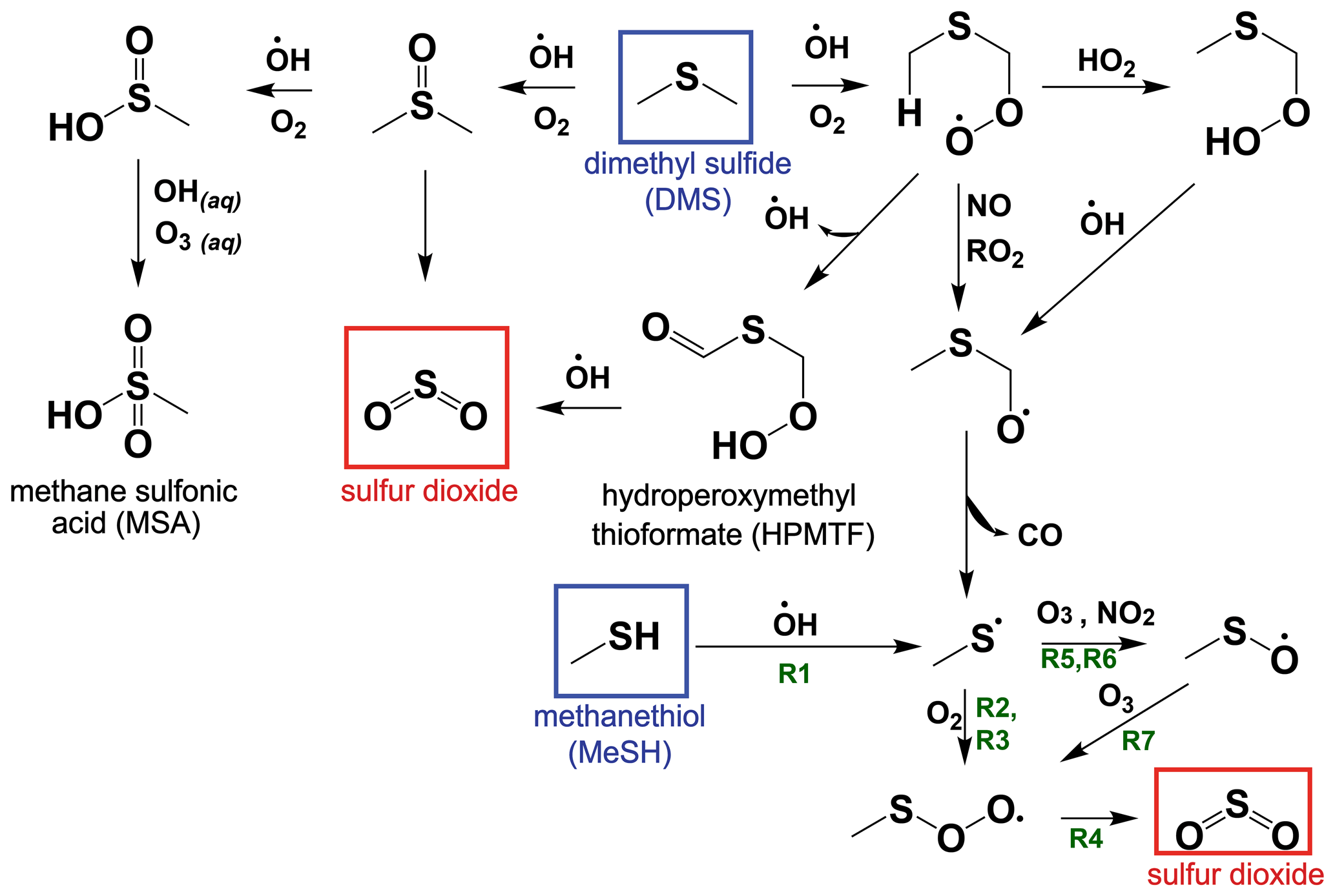
Figure 1 A simplified reaction scheme for the gas-phase oxidation of dimethyl sulfide (DMS) and methanethiol (MeSH) that focuses on pathways to SO₂ production. Reaction (R1) through Reaction (R7) described in Sect. 1.3 are labeled with green text on the schematic. Other chemical pathways including oxidation by halogens and most condensed-phase reactions of DMS and its oxidation products are not shown in this simplified schematic. Refer to Table S1 for a complete list of reactions and rate equations as implemented in this work.

1.4 Study overview

Here we present eddy covariance (EC) flux measurements of DMS and MeSH emissions at a coastal ocean site using a high-sensitivity Vocus PTR-TOF for detection (Krechmer et al., 2018). Results from this study show that emission fluxes of DMS (F_DMS) and MeSH (F_MeSH) were well correlated (R²=0.65) and that F_MeSH is a significant contributor to marine sulfur emissions (mean F_MeSH=0.21 ppt m s⁻¹ compared to mean F_DMS=1.13 ppt m s⁻¹). The average ratio of individual DMS to MeSH flux (F_DMS:F_MeSH) measurements for the full campaign was 5.5 ± 3.0. We assess the impact of the observed large MeSH emission flux on production of SO₂ in the marine atmosphere through a coupled ocean flux–atmospheric chemistry 0-D box model with a newly compiled MeSH oxidation mechanism. Modeling results suggest that MeSH contributes approximately 30 % of instantaneous afternoon SO₂ production ($P_{{\mathrm{SO}}_{\mathrm{2}}}$). Together these results show that MeSH emissions are an important contributor to sulfur budgets in the marine atmosphere, and further field studies and laboratory oxidation mechanism investigations are warranted.

2 Experimental methods

2.1 Scripps Pier flux experiment overview

Measurements of DMS and MeSH gas-phase mixing ratios and EC flux were made continuously from the end of the Ellen Browning Scripps Memorial Pier (hereafter SIO Pier) at the Scripps Institution of Oceanography in La Jolla, CA, USA, during September 2019. SIO Pier is 330 m long and extends over 100 m beyond the wave-breaking zone. The SIO Pier site has been used regularly for EC studies of ocean–atmosphere trace gas exchange (Kim et al., 2014; Novak et al., 2020; Porter et al., 2018; Vermeuel et al., 2020). SIO Pier experiences a characteristic sea breeze circulation pattern during summer where winds are from the ocean at moderate wind speeds (0–6 m s⁻¹) during daytime and are from land at night, which limits nighttime flux determinations. DMS and MeSH were detected with a latest-generation Vocus PTR-TOF instrument (TOFWERK, Aerodyne), with a high-resolution time-of-flight (HTOF) mass analyzer (resolution ca. 5000 MΔM⁻¹ for DMS and MeSH) (Krechmer et al., 2018). The Vocus was housed in a temperature-controlled trailer at the end of the pier and sampled through a 19 m-long perfluoroalkoxy (PFA) inlet (0.625 cm i.d.) enclosed in an opaque housing to prevent photochemistry in the sampling line. The inlet was pumped at 22 slpm, which maintained turbulent flow and short residence times in the sampling line (Reynolds number 4280, calculated volumetric evacuation time 1.7 s). The full inlet line was held at 40 ^∘C, which was always above ambient temperatures to prevent condensation of water vapor on inlet surfaces. A bypass line through the Vocus front end subsampled from the main inlet at 5 slpm through a PFA tee located at the instrument interface. The Vocus subsampled from this bypass at a flow rate of 100 sccm immediately in front of the Vocus capillary inlet into the instrument drift tube. This sampling configuration was used to reduce residence times in the sampling lines as much as possible (total estimated inlet and instrument residence time ∼1.9 s). In addition to the main inlet line, all surfaces in contact with the ambient sample flow, including unions and valves, were composed of PFA or polyetheretherketone (PEEK) in order to minimize known surface artifacts for MeSH sampling except for one stainless-steel union at the Vocus subsampling point (Perraud et al., 2016). The ambient inlet sampling point was collocated with a sonic anemometer recording 3-D winds at 10 Hz (Gil HS-50). The sonic anemometer and Vocus inlet were mounted on a 6.1 m long boom extended beyond the end of the pier to minimize flow distortions from the pier. The inlet was mounted on the boom at a height of 13 m above the mean lower low tide level. Ocean depth below the pier sampling point was ca. 6 m.

The Vocus was operated at a drift tube pressure of 1.5 mbar and an axial electric field gradient of 41.5 V cm⁻¹, resulting in a high overall effective field strength ($E/N$) of 143 Td. Mass spectra were recorded at 10 Hz for the full mass range of 19–500 $m/Q$. The second radio frequency (RF)-only focusing quadrupole in the instrument was operated at an amplitude of 275 V at the start of the campaign before being reduced to 235 and ultimately 215 V later in the deployment. The reduced amplitude on the quadrupole increased transmission of low mass (<50 $m/Q$) ions as described by Krechmer et al. (2018). MeSH ($m/Q$ 49) transmission was increased by 10 % at the reduced amplitude of 215 V, compared to 275 V, which was accounted for in the data processing. Transmission efficiency of DMS was independent of the quadrupole amplitude as its nominal mass ($m/Q$ 63) is larger than the mass discrimination window of the quadrupole. High-resolution peak fitting and integration of the mass spectra were performed in the Tofware 3.2.0 software developed by the instrument manufacturer (TOFWERK).

Additional ancillary measurements made continuously from the pier included O₃ mixing ratios, temperature, relative humidity, and incoming solar irradiance. O₃ mixing ratios were measured at 1 min time resolution (POM, 2B Technologies) in line with the Vocus with a subsampling point immediately downstream of the Vocus subsampling point. Temperature and RH (Vaisala HMP110) were also measured inline downstream of the Vocus subsampling point at 1 Hz time resolution. Incoming total solar irradiance at 1 Hz time resolution (Licor LI-200R) was measured via a sensor mounted on top of the trailer housing the Vocus. Measurements of sea surface temperature (SST), salinity, and chlorophyll are continuously collected at a 1 min time resolution from the end of the pier from an automated shore station operated by the Southern California Coastal Ocean Observing System (Wright, 2016).

2.2 DMS and MeSH calibrations and limit of detections

Instrument calibration factors for DMS were determined during ambient sampling by a two-point standard addition of a DMS gas standard (Praxair, 5.08 ppm ± 5 %) to the full sampling inlet every 2.5 to 4 h. Campaign mean sensitivity to DMS was 3.9 cps ppt⁻¹. Sensitivity to DMS was independent of RH. MeSH was not directly calibrated for during field sampling. Post-campaign calibrations for MeSH were performed in the laboratory using a MeSH compressed gas standard (Airgas, 6.11 ± 5 % ppm) yielding a calibration factor of 1.3 cps ppt⁻¹ for dry conditions. MeSH sensitivity was slightly humidity dependent, resulting in the sensitivity at 80 % RH being 11 % lower than at 0 % RH. Calibrations for MeSH were performed with the same 19 m sampling line and flow conditions used for ambient sampling. We expect that this reduced sensitivity for MeSH at high RH is at least partially due to reactions on inlet surfaces, which is a known complication in MeSH sampling (Perraud et al., 2016). Ambient MeSH calibration factors were determined by scaling the measured in-field DMS calibration factors by the RH-dependent DMS:MeSH sensitivity ratio determined from the laboratory calibrations. We note that the observed sensitivity ratio of DMS:MeSH is different from what would be predicted based on measured proton transfer rate coefficients, which are approximately equal for DMS and MeSH (Williams et al., 1998), emphasizing the need for direct calibration of MeSH.

Instrument backgrounds were determined by overflowing the full inlet line with dry UHP N₂ at the tip of the ambient sampling point. Ambient sampling periods were subdivided into 30 min blocks and were matched to the nearest temporal calibration and background determination point. The campaign mean, median, and interquartile range for DMS were 72.6, 49.2, and 28.0–89.8 ppt, respectively. MeSH mean, median, and interquartile range mixing ratios were 19.1, 13.4, and 7.6–24.5 ppt. Limits of detection (LODs) at a signal-to-noise (S $/$ N) ratio of 3 were 2.6 ppt for DMS and 3.6 ppt for MeSH for a 10 s averaging time following the calculation method of Bertram et al. (2011).

2.3 Eddy covariance flux measurements

2.3.1 Eddy covariance calculation overview

The flux (F) of trace gas across the interface is described by Eq. (1) as a function of both the gas-phase (C_g) and liquid-phase (C_l) concentrations and the dimensionless gas over liquid Henry's law constant (H), where K_t, the total transfer velocity for the gas, encompasses all of the chemical and physical processes that govern air–sea gas exchange (Liss and Slater, 1974).

$$\begin{array}{}\text{(1)}& F=K_{\mathrm{t}}\left({\mathrm{HC}}_{\mathrm{l}}-C_{\mathrm{g}}\right)\end{array}$$

Both DMS and MeSH are persistently supersaturated in the liquid phase, leading to an emission flux to the atmosphere (where a positive flux value indicates emission). Fluxes of DMS and MeSH were measured in the turbulent planetary boundary layer with the well-established EC technique, where F is calculated as the time average of the instantaneous covariances from the mean of vertical wind (w) and the scalar magnitude (x, here either DMS or MeSH) as shown in Eq. (2). Overbars are means, and primes are the instantaneous variance from the mean. N is the total number of data points during the flux-averaging period. Ambient data were subdivided into approximately 30 min flux-averaging periods for the EC flux calculation.

$$\begin{array}{}\text{(2)}& F_x={\displaystyle \frac{\mathrm{1}}{N}}{\sum }_i^N\left(w_i-\overline{w}\right)\left(x_i-\overline{x}\right)=\left(w^{\prime }{x}^{\prime }\right)\end{array}$$

2.3.2 EC flux data processing and quality control

Several standard EC data processing steps, data filters, and quality control checks were applied during flux analysis, including (1) filtering by wind direction for periods of onshore winds (true wind direction 200–360^∘), (2) coordinate rotation of 3-D wind components by the planar fit method to remove unintentional tilts in the sonic mounting and account for local flow distortions (Wilczak et al., 2001), (3) application of a friction velocity (U_∗) threshold of 0.05 cm s⁻¹ to reject periods of low shear driven turbulence, (4) despiking of DMS and MeSH data using a mean absolute deviation filter before the EC flux calculation (Mauder et al., 2013), (5) linear detrending of the scalar time series, and (6) flux stationarity filtering with flux periods rejected if they were non-stationary at a 30 % threshold (Foken and Wichura, 1996). Additional discussion of EC flux processing and quality control steps, including lag time determination, spectral analysis, frequency attenuation corrections, and flux LOD determination, are provided in the Supplement. A total of 304 out of 696 flux measurement periods passed all quality control filters. Campaign mean flux of DMS was 1.13 ppt m s⁻¹, with a mean of individual flux period limits of detection at the 3σ confidence interval of 0.35 ppt m s⁻¹. MeSH mean flux was 0.21 ppt m ms⁻¹ with a mean flux 3σ LOD of 0.11 ppt m s⁻¹.

2.4 Coupled ocean–atmosphere flux chemical box model

2.4.1 Meteorological and chemical constraints

A coupled ocean–atmosphere 0-D chemical box model was developed using the Master Chemical Mechanism (MCM) v3.3.1 (http://mcm.york.ac.uk (last access: 1 April 2022), Jenkin et al., 1997; Saunders et al., 2003) in the Framework for 0-D Atmospheric Modeling (F0AM, Wolfe et al., 2016) with added chlorine chemistry (Riedel et al., 2014). The model was used to assess the impact of observed MeSH emissions on production of secondary marine SO₂. Model ability to reproduce observed diel profiles of DMS and MeSH mixing ratios was also tested. Measured emission fluxes of MeSH and DMS are coupled to the model to set the source term for those molecules. Ambient pressure and temperature data were acquired from the NOAA National Data Buoy Center (stations LJPC1 and LJAC1) as well as from an on-site temperature and relative humidity data logger (OM-62, Omega Engineering). Chemical constraints included coincident measurements of O₃ and nitryl chloride (ClNO₂) measured at the same site in August 2018 (Vermeuel et al., 2020), an assumed OH profile that followed the solar cycle with a peak at 4.0 × 10⁶ molecules cm⁻³, and constant concentrations of other major trace gases as listed in Table S2. A constant first-order dilution loss term was used with a 1 d lifetime to approximate mixing out of the boundary layer. A static boundary layer height (BLH) of 500 m was assumed (Faloona et al., 2005; Stull, 1988; Wei et al., 2018). Clear-sky conditions were also assumed (i.e., no heterogeneous loss from reactive uptake on cloud droplets; Vermeuel et al., 2020). An updated oxidation mechanism for DMS and MeSH was implemented, expanding upon the default DMS oxidation scheme in the MCM v3.3.1 to include oxidation of MeSH to form CH₃S Reaction (R1) and to include HPMTF chemistry, detailed in Table S1. The model was allowed to spin up for 2 d to allow reactive intermediates to reach equilibrium, with all reported values taken from day 3 of the model run.

2.4.2 Box model conditions

Pier Model Case

Two distinct model cases were developed which differ in how they treat the diel profile of F_DMS and F_MeSH. The first (termed the “Pier Model Case”) used the observed diel profile of F_DMS and F_MeSH at Scripps Pier to test model ability to reproduce observed diel profiles of DMS and MeSH gas-phase mixing ratios. Nighttime flux measurements from 23:00 to 09:00 were limited during this study due to persistent offshore wind conditions. Instead, we apply a constant nighttime emission flux taken as the average of the 09:00–10:00 and 21:00–22:00 flux observations for DMS and MeSH. A 3 h moving mean was also applied to the observed diel flux profiles to reduce the influence of experimental variability on the model. This Pier Model Case is used in the analysis of diel profiles presented in Sect. 3.4.

Open Ocean Case

A second case (termed the “Open Ocean Model Case”) was developed to provide a general assessment of the relative contribution of DMS and MeSH emissions to SO₂ production as described in Sect. 3.5. This Open Ocean Case uses fixed values for F_DMS and F_MeSH taken as the campaign mean fluxes rather than a variable diel profile. This case avoids the ambiguity of uncertain nighttime emission flux in the observations and better represents conditions on the open ocean, where there is little diel variability in wind speed, and thus emission fluxes for DMS and MeSH are expected to be relatively constant (Archer and Jacobson, 2005).

3 Results and discussion

3.1 Meteorology overview

Observed meteorology and ocean physical and biogeochemical parameters showed minimal variance over the sampling period. Mean SST during the campaign was 23.3 ^∘C (21.6 to 24.7 ^∘C interquartile range). Observed mean and interquartile ranges of air temperatures and relative humidity were 22 ^∘C (19.5 to 23.6 ^∘C) and 79.9 % (72.3 % to 88.3 %), respectively. Chlorophyll concentrations suggest moderate biological productivity with an observed campaign mean of 1.86 µg L⁻¹ (1.5 to 2.0 µg L⁻¹ interquartile range). O₃ mixing ratios showed a clear diel pattern peaking in mid afternoon with a campaign mean of 32.6 ppbv (27.6 to 38.9 ppbv interquartile range). Wind speeds during onshore wind periods were from 0 to 6 m s⁻¹, typically peaking in late afternoon with a campaign mean of 2.8 m s⁻¹. Clear-sky conditions were observed for most afternoons during the study period, with total solar irradiance peaking near noon. The period from days of year (DOYs) 268–271 saw occasional overcast skies during the afternoon. Light rainfall during the early morning of DOY 271 was the only precipitation during the campaign. Morning and late-evening periods showed occasional presence of marine stratocumulus clouds which drove day-to-day variability in solar irradiance during those times. The campaign time series of wind speed, air temperature, SST, O₃ mixing ratios, solar irradiance, and DMS and MeSH mixing ratios are presented in Fig. 2. Gaps in the DMS and MeSH time series are from instrument maintenance periods, power outages at the site, and periods where the instrument was operated in an alternative sampling mode.

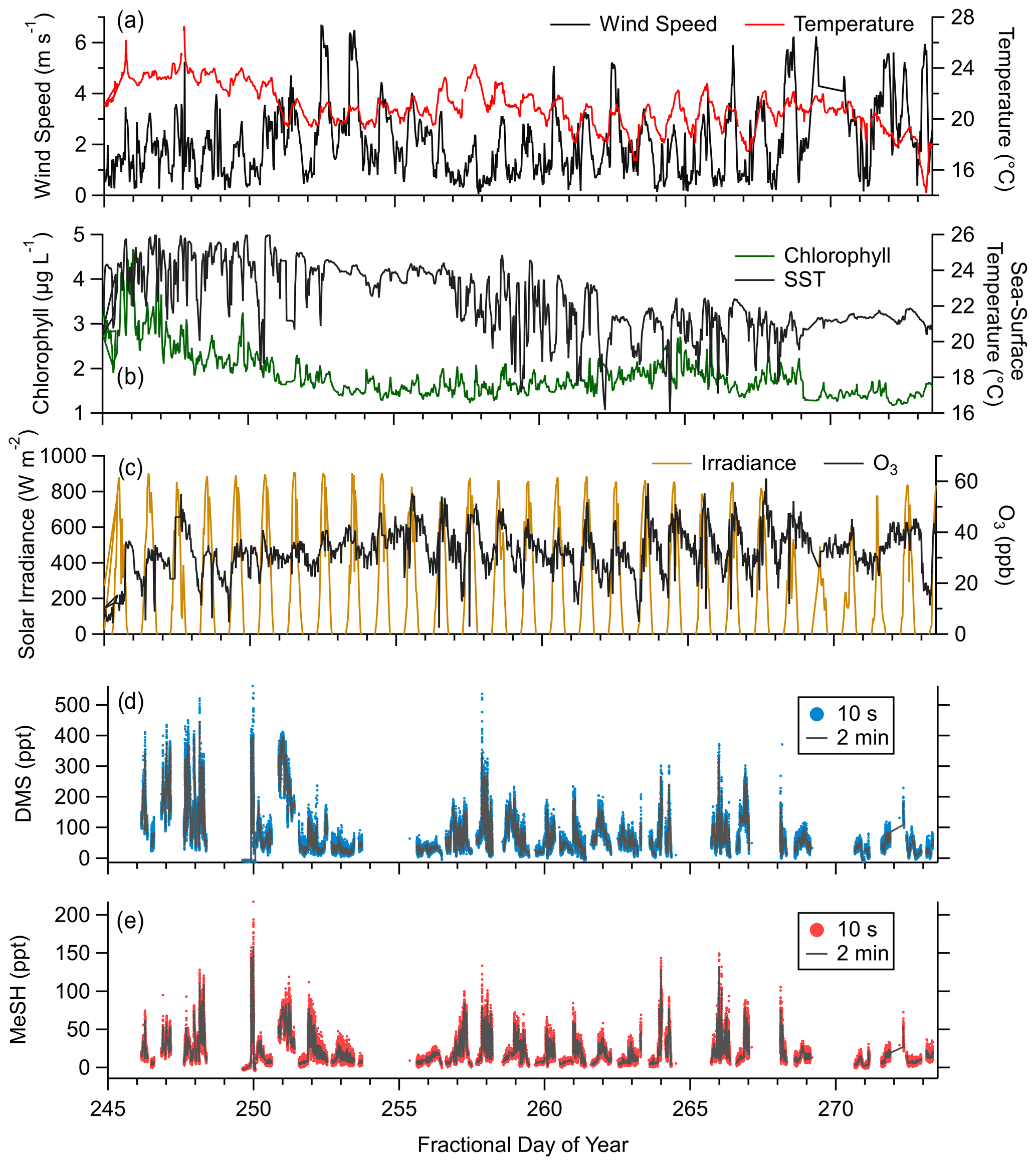
Figure 2 Campaign time series of (a) wind speed and near-surface air temperature, (b) chlorophyll concentration and sea surface temperature (SST), (c) incoming solar irradiance (from 400 to 1100 nm) and ozone (O₃) mixing ratios, (d) mixing ratios of DMS at 10 s and 2 min time resolution, and (e) mixing ratios of MeSH at 10 s and 2 min time resolution.

3.2 DMS and MeSH gas-phase mixing ratios

The campaign mean, median, and interquartile range of DMS mixing ratios were 72.6, 49.2, and 28.0–89.8 ppt, respectively. MeSH mean, median, and interquartile range mixing ratios were 19.1, 13.4, and 7.6–24.5 ppt. Maximum concentrations of DMS and MeSH during the campaign were 562 and 217 ppt, respectively, for 10 s time-averaged data. The correlation of observed DMS and MeSH mixing ratios at a 2 min averaging time colored by the hour of day (local time, UTC − 7) of the observation are shown in Fig. 3. The slope of the correlation was 0.19, with a linear least squares regression coefficient (R²) of 0.61. The ratio of DMS:MeSH mixing ratios reaches a minimum near hours 05:00–07:00 following the build-up of MeSH overnight. Both DMS and MeSH were observed to reach a maximum in concentration at night and minimum concentrations in the early afternoon as shown in the diel profiles in Fig. 4. The observed diel profile is consistent with expectations due to the significantly lower oxidative loss rate at night and has been observed in other studies (Lawson et al., 2020). MeSH varies by approximately a factor of 5 between its diel average maximum and minimum concentration compared to DMS, which varies by approximately less than a factor of 3. The larger diel variability in MeSH is due to its approximately 5 times faster bimolecular rate constant with OH ($k_{\text{OH+MeSH}}=\mathrm{3.3}\times {\mathrm{10}}^{-\mathrm{11}}$ cm³ molecule⁻¹ s⁻¹ at 293 K) compared to DMS ($k_{\text{OH+DMS}}=\mathrm{7.8}\times {\mathrm{10}}^{-\mathrm{12}}$ cm³ molecule⁻¹ s⁻¹ at 293 K), resulting in a lifetime of MeSH to oxidation by OH during the afternoon on the order of 3 h compared to 16 h for DMS (for [OH] $=\mathrm{2}\times {\mathrm{10}}^{\mathrm{6}}$ molecule cm⁻³). In the remote southwestern Pacific Ocean, Lawson et al. (2020) measured mean DMS and MeSH mixing ratios of 208 and 18 ppt, respectively, with maximum concentrations observed at night. They also found that DMS and MeSH were correlated, with a slope of 0.07 and an R² of 0.3 over the full campaign. We observe similar mean MeSH (19.1 ppt), lower DMS (72.6 ppt), and a larger slope for the correlation of DMS and MeSH (slope =0.19) in this study compared to the Lawson et al. (2020) observations. Still, our results show general qualitative agreement with Lawson et al. (2020), with both showing that atmospheric MeSH is present at a significant ratio relative to DMS.

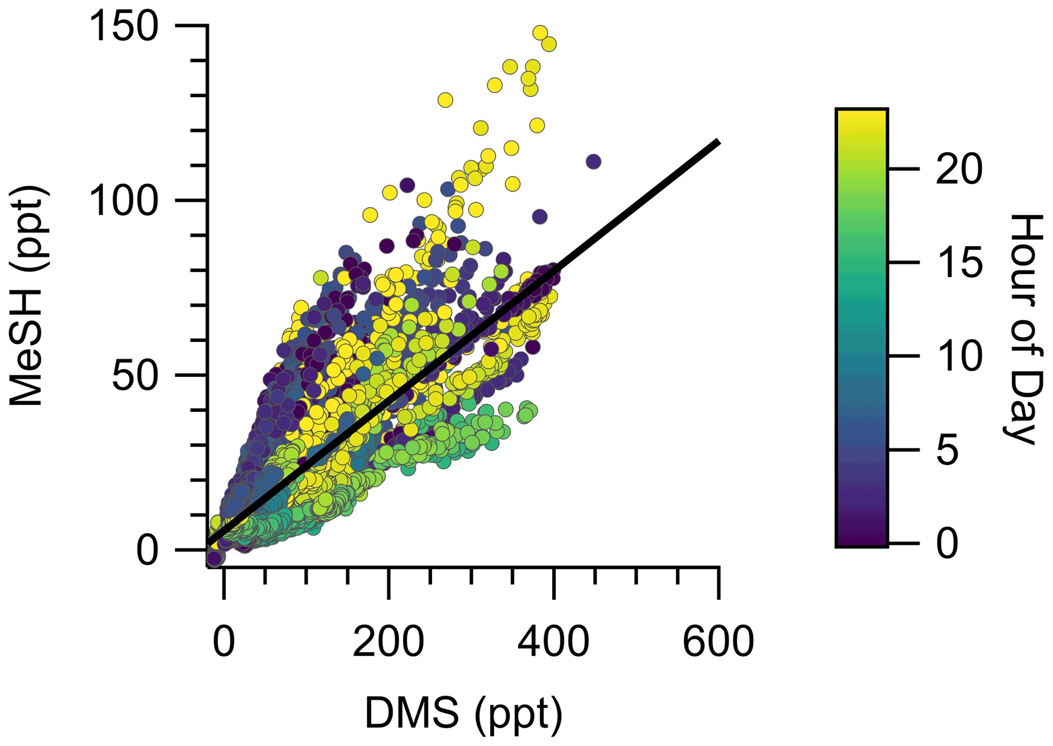
Figure 3 Correlation of DMS and MeSH mixing ratios at a 2 min averaging time colored by hour of day of the observation. Hour of day is in local time (UTC − 7). The linear least squares best fit is plotted as the solid black line. The slope of the best fit line is 0.19, and R²=0.61.

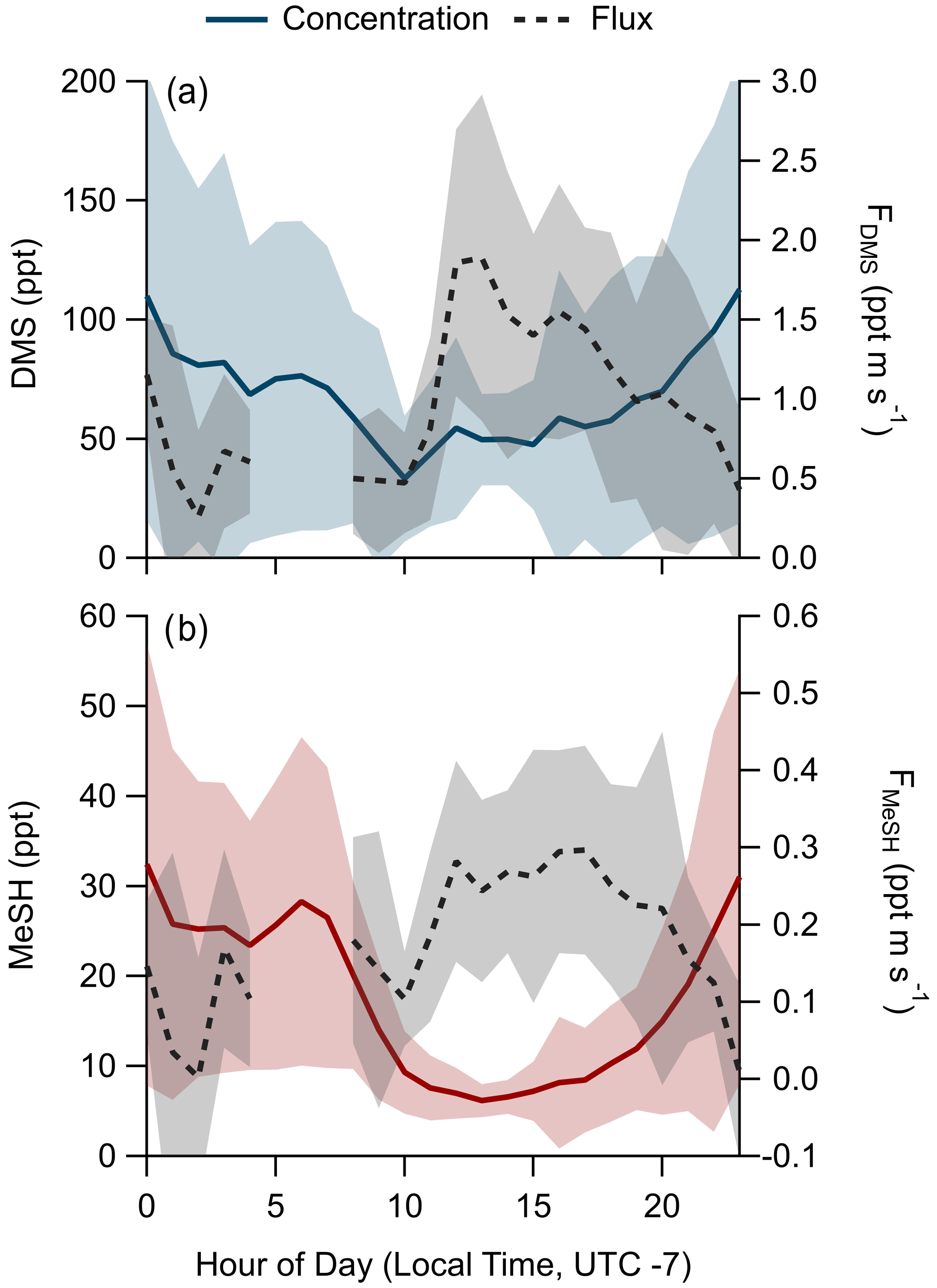
Figure 4 Hourly averaged diel profiles of observed mixing ratios and eddy covariance flux of (a) DMS and (b) MeSH. Shading represents the standard deviation of the binned hourly means. Winds were primarily from the land for hours 00:00–10:00, limiting air–sea flux measurement during those times.

3.3 DMS and MeSH emission flux

A total of 304 valid quality-controlled flux-averaging periods was measured during the campaign. Campaign mean emission fluxes of F_DMS and F_MeSH were 1.13 ppt m s⁻¹ (0.53–1.61 ppt m s⁻¹ interquartile range) and 0.21 ppt m s⁻¹ (0.10–0.31 ppt m s⁻¹ interquartile range), respectively. Both F_DMS and F_MeSH reached a steady maximum between hour of days 10 to 17 as shown in Fig. 4, which corresponds to the typical period of sustained peak wind speed. The magnitudes of both F_DMS and F_MeSH were found to increase with wind speed as shown in Fig. 5, following expectations for supersaturated species at moderate wind speeds where flux magnitude is controlled by physical transfer terms (Carpenter et al., 2012; Huebert et al., 2004; Kim et al., 2017; Marandino et al., 2007). Measurement of F_DMS and F_MeSH during nighttime was limited due to persistent winds from the land at night throughout the campaign. Fewer than 15 % of the valid flux observations were between hours 22:00 and 07:00. Further, those nighttime flux measurements were smaller and showed high variability compared to daytime measurements. DMS and MeSH fluxes were highly correlated with each other (R²=0.65) as shown in Fig. 6a. Campaign mean F_DMS:F_MeSH calculated as the simple mean of the ratio of individual F_DMS and F_MeSH observations was 5.5 ± 3.0. Lawson et al. (2020) calculated the average emission flux of MeSH compared to DMS ($F_{\mathrm{MeSH}}/(F_{\mathrm{MeSH}}+F_{\mathrm{DMS}})$) to be between 14 % and 24 %, where fluxes were calculated from the nighttime accumulation of DMS and MeSH when oxidative loss was assumed to be negligible. In this study using direct eddy covariance flux measurements, we calculate the mean $F_{\mathrm{MeSH}}/(F_{\mathrm{MeSH}}+F_{\mathrm{DMS}}$) to be 16 %, which compares well to the Lawson et al. (2020) result. As shown in Fig. 6b, F_DMS:F_MeSH is partially correlated (R²=0.15) with ocean chlorophyll concentrations. The time series of chlorophyll concentrations shown in Fig. 2b shows that chlorophyll peaked at the immediate start of gas-phase sampling from DOY 245 to 246 at ca. 3.5 to 4 µg L⁻¹ before declining over the course of several days to roughly constant concentrations from 1 to 2.5 µg L⁻¹ over the remainder of the campaign. The profile of chlorophyll suggests a phytoplankton bloom peak, and decay was sampled in the first period of the campaign, which transitioned into a roughly constant moderately biologically productive state for the remainder of the campaign. F_DMS:F_MeSH during the period of peak chlorophyll concentrations over the first 3 d of the campaign (DOYs 245–247) was 10.8 ± 4.4 compared to the mean ratio from the full campaign of 5.5 ± 3.0. The relative production and consumption of DMS and MeSH in seawater is known to be a complex function of the speciation and abundance of phytoplankton and bacteria as well as available organic sulfur and other biogeochemical parameters (Kiene et al., 2000; Kiene and Linn, 2000b). No other measured meteorological parameters, including wind speed, SST, and solar irradiance, showed a significant correlation with F_DMS:F_MeSH. The underlying cause of the correlation between F_DMS:F_MeSH and chlorophyll in our dataset is not clear without additional constraints on the ocean biochemistry. However, this result highlights that biological activity can drive variations in dissolved ratios of DMS and MeSH, resulting in variability in ambient F_DMS:F_MeSH emission ratios, and that further study is needed to elucidate this mechanism and its spatiotemporal variability. Measurements during an induced mesocosm phytoplankton bloom experiment using seawater collected at SIO Pier immediately before this study showed that the ratio of gas-phase DMS to MeSH varied by more than a factor of 5 over the course of a phytoplankton bloom and decay (Kilgour et al., 2022). DMS to MeSH ratios in that study were strongly linked to changes in bacterial sulfur demand and changes in the available pool of dissolved sulfur across the phytoplankton bloom and decay cycle. Sun et al. (2016) have also shown that the bacterium Pelagibacter produces both DMS and MeSH from DMSP, where the relative yield of products is related to the amount of excess DMSP compared to the cellular demand for sulfur for biosynthesis. While induced mesocosm blooms and incubation experiments are not fully representative of the ambient ocean, these results demonstrate the controlling role of ocean biology in F_DMS and F_MeSH and ultimately in marine SO₂ production, which must be better constrained through further ambient observations.

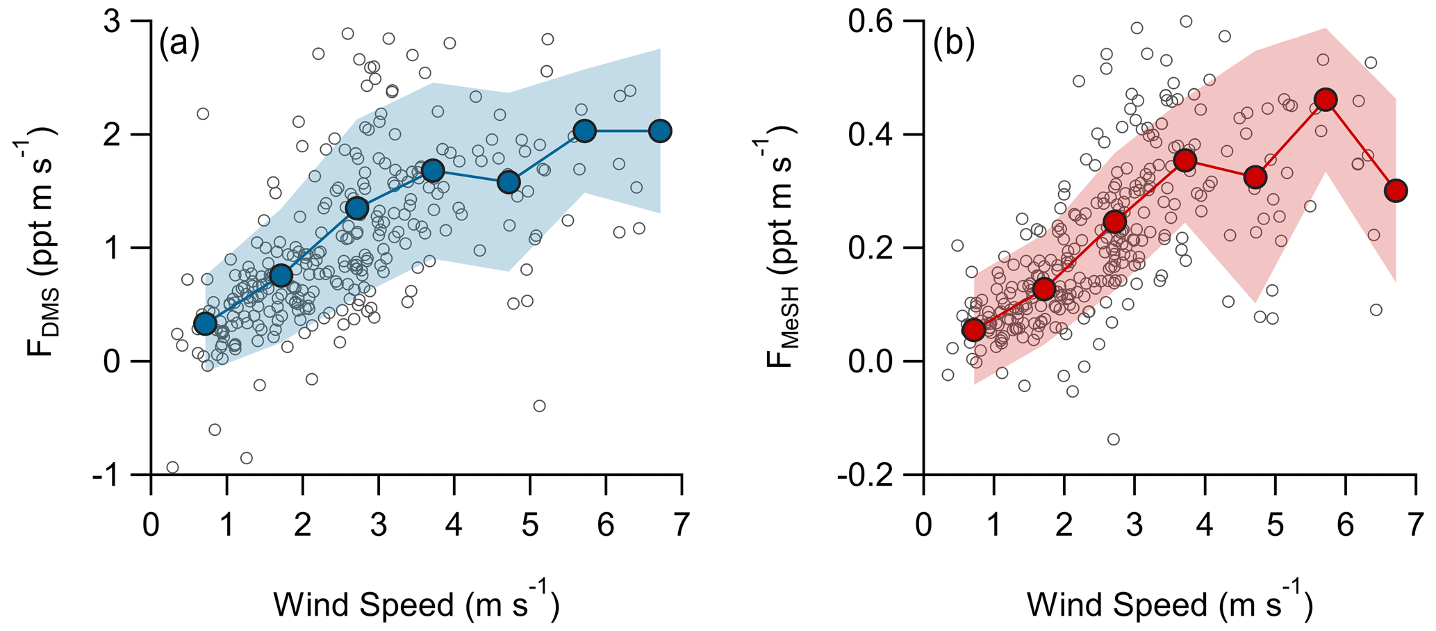
Figure 5 Flux of (a) DMS and (b) MeSH as a function of wind speed. Open circles are individual 30 min data points and closed circles are mean fluxes binned by wind speed at a 1 m s⁻¹ bin spacing. Shaded regions are ± 1σ of the binned mean.

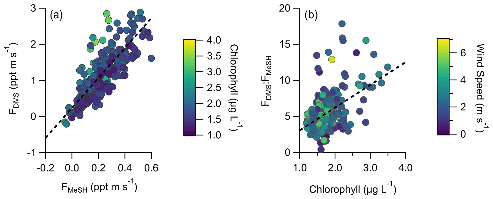
Figure 6 (a) Correlation and linear least squares regressions of measured MeSH and DMS emission fluxes (F_MeSH and F_DMS, respectively). The slope of the best fit line is 4.15, and R²=0.65. (b) Correlation and linear least squares regression of the emission flux ratio of DMS to MeSH (F_DMS:F_MeSH) with ocean chlorophyll concentrations. The slope of the best fit line is 3.15, and R²=0.15. Points in (a) are colored by ocean chlorophyll concentrations and in (b) by mean wind speeds for each flux period.

3.4 Chemical box model comparison to pier observations

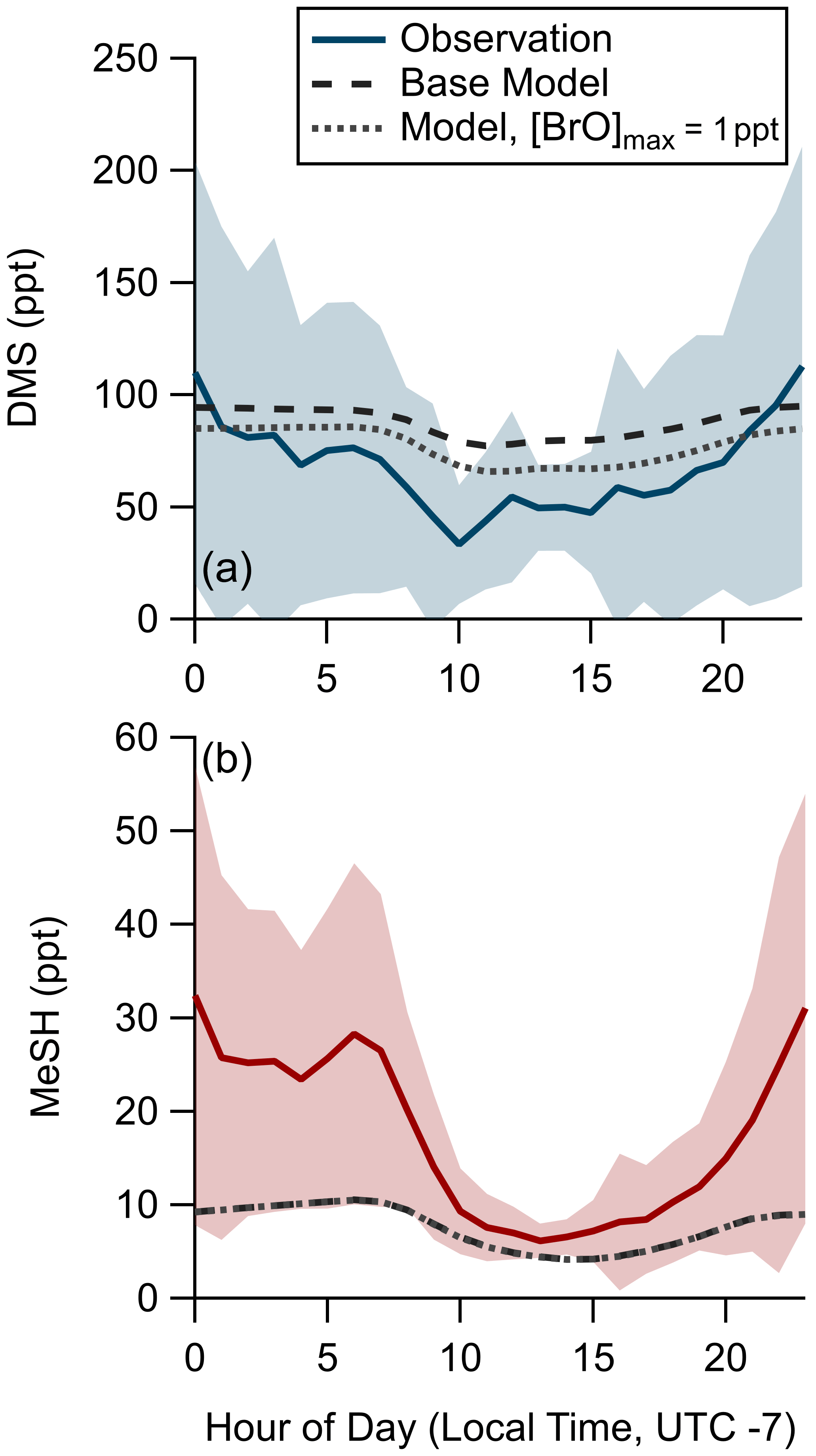
We assessed the ability of the coupled ocean–atmosphere chemical box model described in Sect. 2.4.2 using the Pier Model Case to replicate the observed mean diel profiles of DMS and MeSH mixing ratios from SIO Pier. The model and measurement diel profiles of DMS and MeSH are shown in Fig. 7. For MeSH the model agrees with measurements to within 25 % during daytime hours (10:00–21:00) when direct flux constraints were possible but diverges significantly at night, when the model underpredicts MeSH. DMS is overpredicted by roughly 25 ppt during daytime (hours 09:00 to 20:00) in the model. Modeled DMS also shows less day–night variability in concentration, varying by a factor of 1.25 compared to observations, which vary by approximately a factor of 2. The poorer model performance at night is likely related to diel changes in coastal boundary layer dynamics, including boundary layer height and advection, which are not captured in the model. As noted, nighttime emission fluxes of DMS and MeSH are poorly constrained by the EC flux measurements and may also contribute to the larger disagreement at nighttime. We expect the most informative model test case to be for MeSH mixing ratios during daytime, where the MeSH emission flux is well constrained by measurements and the oxidative lifetime of MeSH is short (<3 h), resulting in modeled MeSH mixing ratios being primarily driven by oxidation and not by the uncertain boundary layer dynamics or nighttime emission fluxes. During daytime modeled and measured MeSH mixing ratios agreed to within 25 %, while DMS mixing ratios were overpredicted by ∼50 %. One additional potential driver of model overprediction of DMS during daytime is the exclusion of BrO chemistry from the base model due to the lack of observational constraints of BrO at the study site. BrO has been suggested to be an important oxidant of DMS which peaks in concentration in the afternoon (Saiz-Lopez et al., 2006, 2008). A model sensitivity run using an afternoon peak BrO concentration ([BrO]_max) of 1 ppt was performed, which brings modeled DMS to within 10 ppt of the observations during daytime but degrades model-to-observation agreement at night. The [BrO]_max of 1 ppt was selected as an intermediate value in the range of measured and modeled BrO in the daytime marine boundary layer; however, mean daytime BrO mixing ratios of up to 4 ppt have been observed in some locations (Mahajan et al., 2010; Saiz-Lopez et al., 2004; Wang et al., 2019). Implementing higher BrO mixing ratios in this model would generally serve to decrease modeled DMS and MeSH mixing ratios, especially during daytime. Daytime MeSH mixing ratios are reduced by less than 0.5 ppt in the 1 ppt BrO sensitivity test, as MeSH oxidation is still dominated by OH. Due to the lack of observational constraint on BrO during our study, we elect to exclude BrO chemistry from the model base case used in subsequent calculations. Inclusion of BrO chemistry would have minimal impact on model MeSH as described and would serve to reduce DMS lifetime, increase the yield of DMSO and MSA from DMS oxidation, and reduce the yield of SO₂ from DMS oxidation. While there are clear uncertainties in this modeling effort, especially during nighttime, the general model ability to reproduce observed DMS and especially MeSH mixing ratios during daytime when we have robust constraints on the emission flux suggests that the DMS and MeSH oxidation mechanism added to the MCM v3.3.1 in this work is suitably accurate for providing meaningful information on the oxidative fate of DMS and MeSH.

Figure 7 Observed and modeled diel profiles of (a) DMS and (b) MeSH mixing ratios.

3.5 Impact of MeSH on marine sulfur dioxide production

Production of SO₂ as a function of F_DMS and F_MeSH was assessed using the Open Ocean Case of the coupled ocean–atmosphere 0-D box model described in Sect. 2.4.2. Chemical box modeling of MeSH emission and gas-phase oxidation suggests that MeSH contributes significantly to marine boundary layer SO₂ concentration. For a model case where F_MeSH is taken to be 0 and F_DMS is taken to be the campaign mean of 1.1 ppt m s⁻¹, modeled afternoon (hours 12:00 to 16:00) mean SO₂ mixing ratio is 29.5 ppt, and the instantaneous SO₂ production rate ($P_{{\mathrm{SO}}_{\mathrm{2}}}$) is 5.8 ppt h⁻¹. When F_MeSH is added to the model at the observed campaign mean of 0.21 ppt m s⁻¹, model afternoon mean SO₂ increases to 46.5 ppt, and $P_{{\mathrm{SO}}_{\mathrm{2}}}$ increases to 8.3 ppt h⁻¹. Model diel profiles of SO₂ mixing ratios and $P_{{\mathrm{SO}}_{\mathrm{2}}}$ with and without MeSH emissions are shown in Fig. 8. In the campaign mean case MeSH emissions contribute 30 % of the overall SO₂ production (or a 43 % increase in total SO₂ production compared to the F_DMS-only case). The model yield of SO₂ from MeSH oxidation was 0.99, which is comparable to an experimentally constrained model determination of the atmospheric yield of 0.98 (Chen et al., 2021). We include the full MeSH oxidation mechanism for completeness due to its overlap with known DMS chemistry and ease of implementation in the box model. However, given our determined model yield of SO₂ from MeSH of 0.99 and a recently determined yield of 0.98 constrained by laboratory oxidation studies (Chen et al., 2021), future modeling efforts may be justified in simplifying this mechanism by including only a direct MeSH + OH → SO₂ reaction at a yield of 1. Prior efforts to constrain the total SO₂ budget in the marine boundary layer required a unit yield of SO₂ from DMS (Faloona et al., 2009), which stands in contrast to the 40 %–80 % range typically determined in laboratory and modeling studies (Faloona, 2009; Gray et al., 2011). This discrepancy has prompted consideration that other potential SO₂ precursors might be present which might reduce the yield of SO₂ from DMS needed to close the SO₂ budget (Bandy et al., 2011). Oceanic MeSH emissions as observed in our study are likely one such additional contributor to secondary marine SO₂ which has not been previously considered. Eddy covariance flux measurements of ocean–atmosphere trace gas exchange have generally been limited to a small set of molecules (e.g., DMS, acetone, methanol, acetaldehyde) (Novak and Bertram, 2020). As demonstrated with the MeSH measurements presented here, marine EC flux observations of new molecules are critical for constraining marine sulfur and volatile organic compound (VOC) budgets. Global spatiotemporal variability of MeSH emission flux magnitude and the ratio of F_DMS:F_MeSH are both highly uncertain due to the sparsity of ambient observations, which will need to be better constrained through future studies.

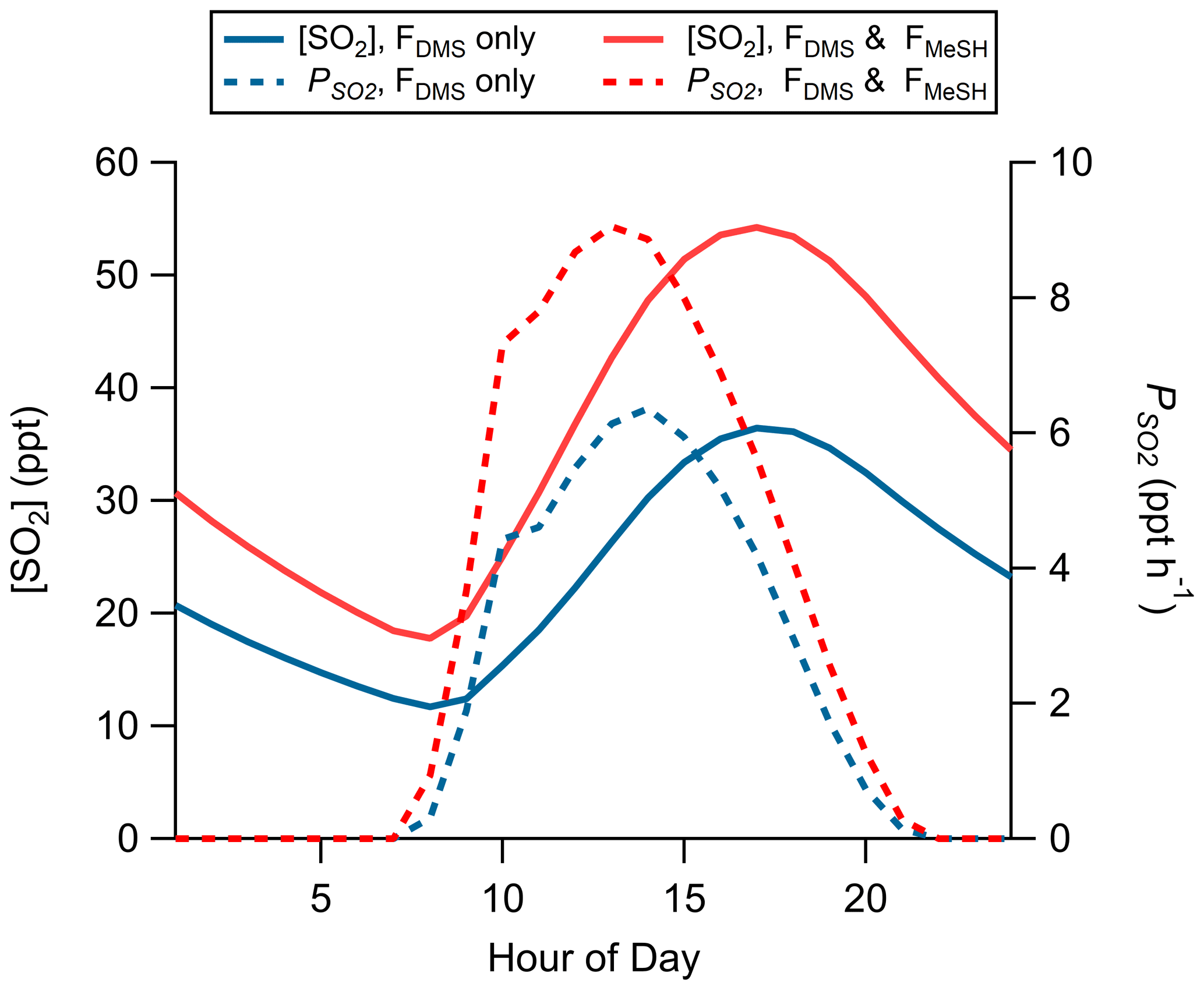
Figure 8 Modeled diel profiles of SO₂ mixing ratios and instantaneous SO₂ production rates ($P_{{\mathrm{SO}}_{\mathrm{2}}}$) for a model case considering only DMS emissions (F_DMS only, blue traces) and one including both DMS and MeSH emissions (F_DMS and F_MeSH, red traces). Emissions were taken as the measured campaign mean flux of DMS and MeSH.

Heterogeneous chemistry of the DMS oxidation product HPMTF is not included in our base model case. HPMTF heterogeneous chemistry has been proposed to be a potentially large sink for HPMTF which would reduce SO₂ production from DMS (Novak et al., 2021; Veres et al., 2020; Vermeuel et al., 2020). These details of HPMTF heterogeneous chemistry do not impact the yield of SO₂ from MeSH described previously but do impact the calculated relative production of SO₂ from MeSH compared to DMS. Inclusion of HPMTF heterogeneous chemistry (at γ=0.01 and an aerosol surface area of 48 µm² cm⁻³) reduces model SO₂ production from DMS to 2.7 ppt h⁻¹ compared to 5.8 ppt h⁻¹ in the model base case. In the HPMTF heterogeneous chemistry case MeSH oxidation accounts for 48 % of marine SO₂ production. Further details on HPMTF chemistry are given in Sect. S5 in the Supplement.

We also note that the yield of SO₂ production from MeSH does not have a temperature dependence, unlike DMS, which may result in MeSH being an especially important source of SO₂ in colder high-latitude regions. At lower temperatures, the DMS OH-addition reaction pathway becomes more favored, resulting in less efficient production of SO₂ from DMS oxidation as production of highly soluble intermediates begins to dominate compared to at higher temperatures. Model calculations presented here used the measured diel temperature profile at SIO Pier during this study, which had a mean of 293 K.

Modeled daytime $P_{{\mathrm{SO}}_{\mathrm{2}}}$ as a function of DMS and MeSH emission flux magnitude is shown in Fig. 9 with the interquartile ranges of F_MeSH and F_DMS measured SIO Pier overlayed as a constraint. These results highlight the potential variability in $P_{{\mathrm{SO}}_{\mathrm{2}}}$ in varying regimes of F_DMS:F_MeSH. Model results were from the base Open Ocean Case described in Sect. 2.4.2. Given the potential biological control on F_DMS:F_MeSH, the temperature dependence of SO₂ yield from DMS, and the impact of HPMTF heterogeneous chemistry on SO₂ yield from DMS, we expect there may be significant temporal and regional variability in the relative contribution of DMS and MeSH to marine $P_{{\mathrm{SO}}_{\mathrm{2}}}$ across the global oceans. This additional SO₂ production from MeSH will likely contribute to new particle formation and growth through enhanced production of sulfuric acid (H₂SO₄), with subsequent impacts on CCN abundance in the MBL. Given the newly determined significance of both MeSH emissions and HPMTF heterogeneous chemistry on marine SO₂ production, a critical reevaluation of the global marine SO₂ budget is likely warranted.

Figure 9 Modeled SO₂ production rate ($P_{{\mathrm{SO}}_{\mathrm{2}}}$) in the marine boundary layer as a function of MeSH and DMS emission fluxes. The interquartile range of measured F_DMS and F_MeSH at SIO Pier is plotted as a black square.

3.6 Limited observational evidence for other volatile organic sulfur compounds

In addition to DMS and MeSH, several other volatile organic sulfur compounds (VOSCs) have been reported to be significant in the marine atmosphere, either from direct oceanic emissions or gas-phase oxidation of precursor species. Recent shipborne observations in the Arabian Sea reported high mixing ratios of dimethyl sulfone (DMSO₂, 40–120 ppt) and methane sulfonamide (MSAM, 20–50 ppt) downwind of a biologically productive upwelling region (Edtbauer et al., 2020). Reported DMS in the same region was from 100 to 300 ppt. The authors in that study propose a direct oceanic emission source of MSAM as there is no known gas-phase oxidation pathway to produce MSAM from DMS. For our observations at Scripps Pier, both MSAM and DMSO₂ were found to have no observable emission flux above the flux limit of detection at either the standard 3σ LOD threshold or a more relaxed 1σ LOD threshold. Gas-phase mixing ratios of MSAM, DMSO, and DMSO₂ were also not found to be significant, with none of those species consistently observed above the 10 s averaging time LOD of 2.4, 7.0, and 9.2 ppt, respectively. All determinations of MSAM, DMSO, and DMSO₂ mixing ratio and LOD assume they have the same detection sensitivity as DMS. Our measurements of DMSO and DMSO₂ are consistent with box model calculated mixing ratios which show hourly maxima of 4.9 ppt and <0.1 ppt for DMSO and DMSO₂, respectively, which are both below the instrument LOD. The box model conditions used were the Pier Model Case with the addition of [BrO]_max of 1 ppt. Oxidation of DMS by BrO favors DMSO and DMSO₂ production, and the inclusion of [BrO]_max of 1 ppt was done as a test of the reasonable upper limit case for DMSO and DMSO₂ production for conditions during this study. DMSO₂ was also measured at Palmer Station, Antarctica, in January to February of 1994 with mean and median mixing ratios of 1.7 and 1.3 ppt, respectively (Berresheim, 1998). The higher DMSO₂ mixing ratios observed in that study are likely at least in part due to the much lower temperatures (mean 274.5 K), where the DMS + OH addition channel forming DMSO and DMSO₂ is more favored. Dimethyl disulfide (DMDS, CH₃S₂CH₃) was also not consistently observed above the LOD in our measurements.

While a direct oceanic emission source of MSAM to the atmosphere has been proposed (Edtbauer et al., 2020), we did not measure a detectable MSAM emission flux in this study. As noted by Edtbauer et al. (2020), given the Henry's law constant of MSAM ($K_{\mathrm{H}}=\mathrm{3.3}\times {\mathrm{10}}^{\mathrm{4}}$ M atm⁻¹), the waterside concentration of MSAM necessary to drive a net emission flux of MSAM to the atmosphere is on the order of 1700 nM. Given that maximum total dissolved organic sulfur (DOS) in ocean surface waters is on the order of 200 nM (Ksionzek et al., 2016), even if all surface ocean DOS was in the form of MSAM, we still would not expect an emission flux of MSAM to the atmosphere. This exercise suggests MSAM may instead be formed through an unknown reaction pathway in the atmosphere which was active in the Arabian Sea but not in our observations at SIO Pier in coastal southern California. Taken together, our observations indicate that MSAM, DMSO, and DMSO₂ emission fluxes and mixing ratios were small at the SIO Pier site, consistent with model calculations.

This discussion on the lack of observations of other VOSCs only extends to molecules that are detectable with the Vocus PTR instrument, such as DMSO, DMSO₂, MSAM, and DMDS. For example, it does not include inorganic sulfur-containing molecules such as carbonyl sulfide (OCS) and carbon disulfide (CS₂) which also have a known oceanic source but are not readily detectable by PTR. In particular, our measurements do not include the recently observed DMS oxidation product HPMTF, which was found to be a globally ubiquitous sulfur reservoir from airborne observations in the marine atmosphere (Veres et al., 2020) and in prior surface observations at SIO Pier (Vermeuel et al., 2020). HPMTF is not detectable with the Vocus PTR ion chemistry used in this study. HPMTF was previously observed in the summer of 2018 at the SIO Pier site to have a strong diel profile, peaking in the early afternoon with an average daytime mixing ratio of 12.1 pptv (Vermeuel et al., 2020). While observations of HPMTF were made 1 year prior to the DMS and MeSH observations reported here, it suggests that HPMTF may comprise up to 10 %–20 % of the total daytime VOSC concentration at this site during summer.

4 Conclusions

We present the first direct eddy covariance flux measurement of MeSH emissions from the ocean which show that MeSH emissions account for a mean of 16 % ($F_{\mathrm{MeSH}}/(F_{\mathrm{MeSH}}+F_{\mathrm{DMS}})$) of emitted volatile organic sulfur measurable with the Vocus PTR-ToF during this study. DMS and MeSH emission fluxes were correlated with each other (R²=0.65), consistent with their shared oceanic source from the degradation of DMSP. Measured F_DMS:F_MeSH was found to have a weak correlation (R²=0.15) with chlorophyll concentrations, which highlights the need for further study of biogeochemical cycling in the ocean surface which may drive significant spatiotemporal variability in F_MeSH. The atmospheric implications of ocean MeSH emissions were assessed by development of a MeSH oxidation mechanism and incorporation into a coupled ocean–atmosphere 0-D chemical box model. Modeling results show that oxidation of MeSH by OH produces SO₂ at a high yield (∼99 %) and is an important contributor to SO₂ production in the marine atmosphere, driving an increase in afternoon $P_{{\mathrm{SO}}_{\mathrm{2}}}$ of 2.5 ppt hr⁻¹ corresponding to 30 % of total afternoon SO₂ production rates. In a model case including HPMTF heterogeneous uptake to aerosols, SO₂ yield from DMS is reduced and MeSH becomes even more important, accounting for 48 % of marine SO₂ production. Taken together, these results demonstrate that MeSH is an important contributor to volatile sulfur budgets in the marine atmosphere and that further studies are needed to constrain spatiotemporal trends of MeSH emission and oxidation relative to DMS.