Quantification of methane emissions from hotspots and during COVID-19 using a global atmospheric inversion

Concentrations of atmospheric methane (CH₄), the second most important greenhouse gas, continue to grow. In recent years this growth rate has increased further (2020: +15.6 ppb), the cause of which remains largely unknown. Here, we demonstrate a high-resolution (∼80 km), short-window (24 h) 4D-Var global inversion system based on the ECMWF Integrated Forecasting System (IFS) and newly available satellite observations. The largest national disagreement found between prior (5.3 Tg per month) and posterior (5.0 Tg per month) CH₄ emissions is from China, mainly attributed to the energy sector. Emissions estimated from our global system are in good agreement with those of previous regional studies and point source-specific studies. Emission events (leaks or blowouts) > 10 t CH₄ h⁻¹ were detected, but without appropriate prior uncertainty information, were not well quantified. Our results suggest that global anthropogenic CH₄ emissions for the first 6 months of 2020 were, on average, 470 Gg per month (+1.6 %) higher than for 2019, mainly attributed to the energy and agricultural sectors. Regionally, the largest increases were seen from China (+220 Gg per month, 4.3 %), with smaller increases from India (+50 Gg per month, 1.5 %) and the USA (+40 Gg per month, 2.2 %). When assuming a consistent year-on-year positive trend in emissions, results show that during the onset of the global slowdown (March–April 2020) energy sector CH₄ emissions from China increased above expected levels; however, during later months (May–June 2020) emissions decreased below expected levels. Results for the first 6 months of 2019/20 suggest that the accumulated impact of the COVID-19 slowdown on CH₄ emissions from March–June 2020 might be small relative to the long-term positive trend in emissions. Changes in OH concentration, not investigated here, may have contributed to the observed growth in 2020.

1 Introduction

Atmospheric methane (CH₄) as a long-lived greenhouse gas (GHG) has contributed to ∼23 % of the additional radiative forcing since 1750 (Etminan et al., 2016), second only to CO₂. Near-surface concentrations have more than doubled since the pre-industrial era, with the global average dry air mole fraction reaching 1891 ppb in 2020 (NOAA, 2021). This growth can mainly be attributed to increased anthropogenic emissions from agriculture, biomass burning, fossil fuel extraction and use, and waste (Etheridge et al., 1998).

The reduction in global human activities, triggered by the COVID-19 pandemic, provided an opportunity to assess the impact of potential rapid climate mitigation strategies to reduce GHG emissions (Diffenbaugh et al., 2020). The sectors most obviously affected by the slowdown, e.g. transport and industry, are directly associated with fluxes of short-lived pollutants (Ming et al., 2020) and CO₂ (Le Quéré et al., 2020), and less so CH₄ (Forster et al., 2020). The change in energy and fuel demand is estimated to have reduced oil and gas CH₄ emissions by 10 % for 2020 compared with 2019 (IEA, 2021). Similarly, a recent study found reduced emissions from the largest oil-producing basin in the USA, the Permian Basin, between April and May of 2020 (Lyon et al., 2021). Despite this, during 2020 atmospheric concentrations of CH₄ grew by 15.6±0.4 ppb, the largest amount since records began in the early 1980s (NOAA, 2021). An alternative hypothesis is that a reduction in demand could have increased venting when extracting fossil fuels, resulting in increased atmospheric concentrations. The remaining CH₄ source sectors were not expected to have been noticeably impacted by changes in activity during the slowdown. The reduced emissions of OH-forming nitrogen oxides (NO_x) during the slowdown may have reduced the CH₄ sink (Stevenson et al., 2021); however, another recent study suggests that this impact might only have accounted for, at most, a 2-ppb growth, which equates to ∼35 % of the difference in growth between 2019 and 2020 (Weber et al., 2020).

The relatively large atmospheric variability of CH₄ concentrations and relatively accurate available measurements allow for the quantification and attribution of emissions using inverse modelling based on both in-situ (e.g. Wilson et al., 2016; McNorton et al., 2018) and satellite observations (e.g. Bergamaschi et al., 2009; Maasakkers et al., 2019). Global atmospheric flux inversions (e.g. Segers and Houweling, 2018; Qu et al., 2021) are typically performed at a coarse spatiotemporal resolution (∼ monthly, >1^∘), for which localised events (e.g. leaks and blowouts) are difficult to detect. Additionally, previous attempts to quantify emissions have been restricted by limited surface and satellite observations. In 2002, the Scanning Imaging Absorption spectrometer for Atmospheric CartograpHY (SCIAMACHY) provided the first total column CH₄ (XCH₄) measurements from space. These observations were superseded by the Infrared Atmospheric Sounding Interferometer (IASI) in 2006 and the Greenhouse gases Observing SATellite (GOSAT) in 2009, offering higher sensitivity and spatial resolution (∼10 km). GOSAT is limited by a relatively narrow spatial sampling restricting the coverage. Both instruments have been used to constrain CH₄ surface fluxes in inversion studies (e.g. Frankenberg et al., 2005; Maasakkers et al., 2019). The TROPOspheric Monitoring Instrument (TROPOMI) instrument on-board Sentinel-5P, launched in 2017, provides global high-resolution (∼7 km) XCH₄ observations with an improved spatiotemporal coverage and precision (Veefkind et al., 2012; Hu et al., 2018). These newly available observations provide the opportunity to detect CH₄ hotspots (Barré et al., 2021) and potentially constrain CH₄ fluxes at high spatiotemporal resolution (Pandey et al., 2019; Zhang et al., 2020).

This study presents and evaluates the new capabilities introduced in the European Centre for Medium-Range Weather Forecasts (ECMWF) Integrated Forecasting System (IFS) to estimate emissions of greenhouse gases and atmospheric pollutants using satellite observations of their atmospheric concentrations. The system is being developed within the framework of the EU-funded Copernicus CO₂ project (coco2-project.eu, 2021) and its precursor, the CO₂ Human Emission project (Balsamo et al., 2021) as the global prototype for a new Copernicus anthropogenic CO₂ emissions monitoring and verification support capacity (Janssens-Maenhout et al., 2020). Here, we focus on anthropogenic CH₄ emissions, as they offer a useful testbed for the future CO₂ system for three main reasons. First, relatively accurate remote-sensing observations of CH₄ are available at a high spatiotemporal resolution. Second, the atmospheric gradients are larger for CH₄, providing a suitably high sensitivity of concentration to emissions. Third, the anthropogenic contribution to fluxes is comparable with the natural component, whereas for CO₂ the anthropogenic component is considerably smaller. We address three main outstanding questions. First, are CH₄ emission hotspots quantifiable using multiple sensors and a high-resolution global short-window 4D-Var system when accounting for meteorological errors? Second, how well do concentrations generated using posterior emission estimates agree with independent observations and existing studies? Third, is the system capable of assessing potential longer-term trends during the COVID-19 pandemic slowdown?

The following sections, Sect. 2.1 and 2.2, outline model methodology, detailing the 4D-Var inversion system used and prior assumptions made. Section 2.3 describes the observations assimilated into the inversion system. Section 3.1 identifies suitable prior uncertainty assumptions in CH₄ fluxes. Section 3.2 provides a global overview of posterior fluxes and the relative changes from prior estimates. Section 3.3 evaluates the system using a range of regional and persistent point source case studies. Section 3.4 investigates the feasibility of quantifying emissions at both a high spatial and temporal resolution using case studies. Section 3.5 investigates the influence of the global slowdown triggered by the COVID-19 pandemic on CH₄ emissions. Section 4 discusses the findings and relevance to the wider community including limitations and suggestions for future work.

2 Methods

2.1 Forward model

The ECMWF global Integrated Forecasting System (IFS), which provides the operational Copernicus Atmosphere Monitoring Service (CAMS, https://atmosphere.copernicus.eu/, last access: 15 January 2022) greenhouse gas (GHG) forecast (Agustí-Panareda et al., 2019), was used to generate the forward model integrations used in this study. These were performed from January to June of 2019 and 2020, with additional case study simulations performed for June 2018, November 2019 and July to September of 2020. Computational cost prevented simulating the full period (2018–2020). Simulations were performed using a horizontal cubic octahedral reduced Gaussian grid (TCo399: ∼25 km) and 137 vertical levels with coupled meteorology at operational forecast timesteps of 15 min and 3-hourly output.

Monthly gridded prior estimates of anthropogenic emissions were taken from the CAMS global emissions product, CAMS-GLOB-ANT v4.2, (Granier et al., 2019), which combines existing products (e.g. EDGAR: Crippa et al., 2018; CEDS: Hoesly et al., 2018). The Global Fire Assimilation System (GFAS) provided daily biomass burning emissions (Kaiser et al., 2012). We used a monthly climatology of wetland emissions based on the LPJ-WHyMe model (Spahni et al., 2011). Remaining fluxes from oceans (Lambert and Schmidt, 1993; Houweling et al., 1999), termites (Sanderson, 1996) and wild animals (Houweling et al., 1999) were used at the highest available spatiotemporal resolution.

The atmospheric CH₄ sink comprised of a monthly mean climatological loss rate field (Bergamaschi et al., 2009), which represents loss reactions with hydroxyl, chlorine and atomic oxygen radicals. A gridded surface soil sink was also used (Ridgwell et al., 1999). Initial conditions for the 3D atmospheric state of CH₄ were taken from the CAMS CH₄ inversion product (Segers and Houweling, 2018).

2.2 Inverse model

2.2.1 4D-Variational inversion

We used the 4D-Var IFS system, cycle 47R1, employed operationally at ECMWF between June 2020 and May 2021. More detailed information on the IFS 4D-Var system can be found in Rabier et al. (2000) and Courtier et al. (1994). The incremental algorithm used consists of solving a series of quadratic minimisation problems (inner-loop) constructed by linearising the initial (non-linear) cost function around updated estimates of the state vector (outer-loop). To constrain surface emissions, the state vector is augmented by a parameter control vector that consists of a 2D scaling factor applied to a prior emission inventory (see Sect. 2.2.2), based on Massart et al. (2021). In our configuration, the posterior scaling factors are optimised on a regular 2D grid (∼80 km) within a 24-h window and then applied to the prior emission inventory defined on a grid of ∼10-km resolution (Fig. 1). Prior emission errors are assumed to be independent between 24-h inversion cycles (i.e. each 24-h inversion uses the same uniform scaling factor of 1 and the same prior errors). This choice was driven by the lack of information about temporal error correlations in current prior inventories. Currently, the error covariance for the CH₄ initial state vector is taken from a climatology and fixed in time (Fig. S3). As a result, posterior errors in methane emissions and 3D state are not propagated forward across data assimilation cycles in this configuration, which is a technical limitation of our current system and will be addressed in subsequent versions. We use an online 4D-Var data assimilation system, where the meteorological fields are part of the control vector and optimised jointly with the emission scaling factors. As a result, the transport errors associated with uncertainties in the initial conditions of the meteorological variables are accounted for in our inversion. This is in contrast with widely used offline inversion systems, wherein transport errors are typically prescribed on an ad-hoc basis and fixed. Note that in our experiments the background errors for the meteorological variables at the initial time are constructed based on a climatology, and therefore are not flow-dependent.

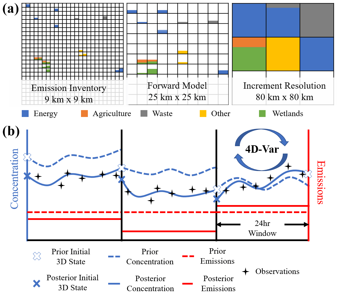
Figure 1 (a) Schematic of different resolutions used in the inversion shown by pseudo-data for five sectors. The magnitude of prior emissions at ∼9 km (left panel) and those same emissions used as input to the forward model at ∼25 km (middle panel). The inversion increment at ∼80 km, resulting scaling factors are applied to all sectors within the grid cell, the boxes indicate relative contribution per sector (right panel). (b) Schematic of inversion setup using the 24-h window, correcting for the initial 3D state, emissions, and initial conditions in the prior of the subsequent window.

The scaling factors derived from the inversion were applied to sector-specific prior maps for source attribution. A caveat to this approach is the assumption that co-located sectors have the same scaling factor applied, which can only be overcome with the use of co-emitted species observations such as ethane or isotopologues (e.g. McNorton et al., 2018). However, this is unlikely to noticeably impact these results as at the relatively high increment resolution used (∼80 km) CH₄ sectors are rarely co-located. Missing sources in the prior are also not accounted for when using a posterior scaling factor.

2.2.2 Prior information

Anthropogenic sector-specific grid cell uncertainties, taken from Maasakkers et al. (2016), provided the initial prior estimate for countries with well-developed statistical infrastructures or Annex I countries (IPCC, 2006). For Non-Annex I countries, the same sector-specific uncertainties were further increased by 50 %. Globally, constant wetland uncertainties were estimated at 58 %, taken as the standard deviation from the WetCHARTs ensemble (Bloom et al., 2017). We assume the standard deviation of the WetCHARTs ensemble to provide a reasonable uncertainty estimate of the LPJ-WHyMe emissions used here. Initially, all other biogenic uncertainties were estimated as 100 %. The atmospheric sink was not optimised by the inversion. Sensitivity experiments where prior errors were perturbed and validated against independent observations were used to evaluate prior uncertainty assumptions (Table S1 in the Supplement). Given that anthropogenic emissions are typically from point sources (e.g. fossil fuel extraction), we assumed no spatial prior error correlation given that the derived increments are at ∼80 km. Wetland emissions would typically require defined spatial correlations; however, given the uncertainty of these structures, the focus of this study being anthropogenic emissions and limited occurrences of co-located emissions from wetland and anthropogenic sources we have chosen to omit these for simplicity. Total grid cell uncertainties, used in the control vector, were calculated using the error propagation method. All prior uncertainties are assumed to have a log-normal distribution to prevent negative emissions.

2.3 Observations

The observations used in the meteorological component of the IFS 4D-Var system include satellite radiances, conventional ground-based and radiosondes, and aircrafts and ships data, for which the coverage and quality is constantly monitored prior the assimilation. With specific focus on CH₄, the TROPOMI instrument on-board the Sentinel-5 Precursor satellite provides near-global daily coverage of XCH₄ with a nadir ground pixel size of 7 km × 7 km and near-surface sensitivity (Veefkind et al., 2012; Lorente et al., 2021). We used operational observations, which became available in April 2018 and were bias corrected, as in Barré et al. (2021). An example representation of daily satellite coverage, which is applicable within a 24-h 4D-Var window, is shown in Fig. S1 in the Supplement. TROPOMI uncertainties (<1 %) provided as part of the CH₄ product were applied within the minimisation routine and averaging kernels were used (Hasekamp et al., 2019). Additional XCH₄ observations from IASI and GOSAT, and their associated uncertainties of ∼2 % and <1 %, respectively, are assimilated into the system to provide additional constraints as described by Massart et al. (2014). Poor quality data are removed based on the provided quality flags.

3 Results

Several simulations were performed. First, a suite of sensitivity experiments was performed to identify an appropriate prior flux uncertainty (Sect. 3.1). This was then used to investigate global emissions (Sect. 3.2), specific emission events (Sect. 3.3 and 3.4) and perform comparative source attribution of CH₄ fluxes during the COVID-19 global slowdown (Sect. 3.5). A full list of simulations is provided in Table S1. Between mid and late March 2020 most of the countries in the world implemented slowdown measures, which reduced socioeconomic activities (Hale et al., 2021). These measures typically lasted until May or June when certain activities were progressively reintroduced, although not to pre-slowdown levels. China is a slight exception, with an earlier slowdown occurring from the end of January. To investigate the impact of these measures on CH₄ emissions, relative to previous years, we perform simulations from January to June for 2019 and 2020. We assume that January and February were business-as-usual months for both 2019 and 2020 and that the relative difference in emissions for these two months between each year represents the long-term trend in emissions.

3.1 Evaluation

To assess the suitability of our prescribed prior error in CH₄ emissions, six sensitivity inversions with a range of uncertainties were performed (see Table S1). We also performed an additional experiment where only the initial 3D atmospheric concentration of CH₄ was optimised. Optimised emissions were then used in forward model simulations, which were evaluated against XCH₄ measurements from 16 Total Column Carbon Observing Network (TCCON) sites (Wunch et al., 2011). TCCON averaging kernels were applied to model profiles as described in Massart et al. (2016). Results show improved performance when including flux scaling factors in the control vector compared with only optimising the initial 3D-state (Fig. S2). When evaluating XCH₄ concentrations simulated with optimised emissions, the lowest all-site average standard error (6.8 ppb) and absolute mean bias (7.52 ppb) was found for the mapped prior error described in Sect. 2.2.2. Using the mapped prior error resulted in a lower standard error in 12 of the 16 sites when compared with the control; furthermore, the absolute mean bias was improved at 10 of the 16 sites. The mapped prior error also produced the highest all-site average R-value (0.74), an improvement compared with the control at 9 of the 16 sites. All subsequent experiments used the mapped prior uncertainty, typically ranging from 50 to 150 %.

3.2 Global emission estimates

As human activities changed in 2020 in response to the COVID-19 pandemic we first investigated the difference between prior and posterior emissions for the first half of a business-as-usual year, 2019. Emissions were estimated using the 4D-Var global inversion system described in Sect. 2.2 from January to June 2019. The resulting fire and wetland emissions are likely to be an inaccurate estimate of annual emissions because of the strong seasonality of both sources. TROPOMI observations do not provide full global coverage within our 24 h 4D-Var window, resulting in emissions not being constrained over large areas. To produce meaningful spatiotemporal budgets of posterior emissions the posterior error covariance should be accounted for. Because this latter quantity is currently lacking in our system, we chose to compute posterior emission budgets based on a subset of grid cells that are significantly constrained by the observations. With this aim in mind, in our analysis, grid cells whose distance to an observation were greater than 1^∘ were discarded. When considering monthly average emissions, the difference in coverage between years is unlikely to significantly impact the results, assuming that the variability within a single month is small. For each selected grid cell, we apply the monthly mean posterior scaling factor to our prior emission inventory to provide a posterior emission estimate. Globally, we found that total average posterior emission estimates (44.0 Tg per month) for 2019 were 0.4 Tg per month smaller than prior estimates (44.4 Tg per month). Within national boundaries, both negative and positive adjustments in emissions often occur (Fig. 2b). Moreover, we found that when averaged over the 6-month period, considerable changes, relative to the prior, are from anthropogenic sources (−0.4 Tg per month).

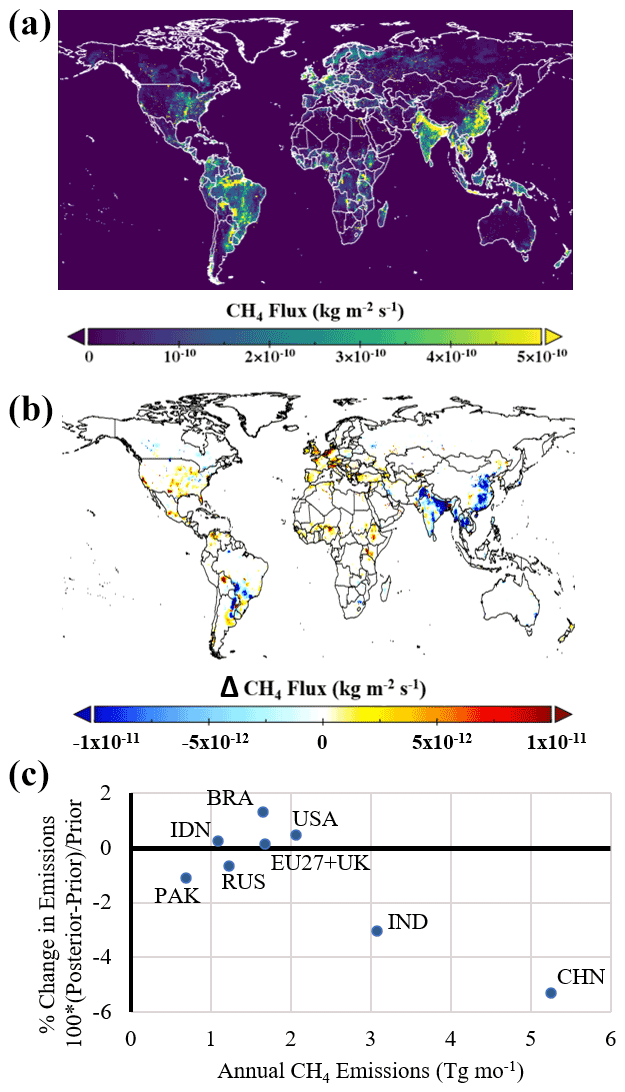
Figure 2 (a) Global annual mean prior CH₄ emissions for 2019 taken from CAMS. (b) Difference between posterior and prior emissions averaged between January and June 2019, derived from the IFS inversion. (c) Posterior adjustment, as a percentage of prior, in anthropogenic CH₄ emissions per country.

On national scales, for the 6-month period, anthropogenic emission differences between the prior (5.3 Tg per month) and the posterior (5.0 Tg per month) were found to be largest over China (Fig. 2c). The potential overestimation in bottom-up emission estimates from China is well documented (e.g. Cheewaphongphan et al., 2019), although the magnitude of this overestimation is uncertain. Using prior emission maps, we distributed total posterior emissions into six sector-specific categories: energy, agriculture, waste, other anthropogenic (industrial, residential and transport sectors), wetlands and fires. In agreement with multiple inverse studies (e.g. Deng et al., 2022) most of the overestimated emissions from China are found to originate from the energy sector (0.2 Tg per month) and specifically from the coal mining regions of Inner Mongolia, Shaanxi and Shanxi. Relative to the prior, posterior emissions are reduced from India (−3.0 %) and Pakistan (−1.1 %), increased from Brazil (+1.3 %) and less than 1 % different for the USA (0.5 %), Indonesia (0.3 %), EU27 + UK (+0.1 %) and Russia (−0.7 %). Except for Russia and Indonesia, these bring emission estimates in closer agreement with other top-down studies (e.g. Deng et al., 2022).

3.3 Emission estimates for regions and point sources

The feasibility of detecting and quantifying emission hotspots on a global scale using a relatively high resolution increment grid (∼80 km, daily), a high-resolution prior emission grid (∼9 km, monthly) and multi-sensor data was evaluated using previously documented case studies (e.g. Zhang et al., 2020; Varon et al., 2020). Preliminary work by Barré et al. (2021) combined high-resolution IFS forecasts (∼9 km) with TROPOMI observations to detect missing emission sources based on a statistical analysis; here, we attempted to extend this to the quantification of emissions in a robust atmospheric transport inversion framework. To filter posterior estimates, which provided little or no added information, we omitted daily grid cells associated with poor observation constraints (see Fig. S1). When comparing our results with those of other studies, and in the absence of a formal posterior uncertainty estimate, the sampling bias introduced by this filtering method may introduce additional uncertainties. Future developments will account for posterior error reduction in our analysis. Efforts are ongoing to include an ensemble-based estimate of the posterior emission errors in our system to provide a more robust evaluation. Posterior emissions and comparisons with existing studies for several case studies are provided in Table 1.

Table 1 Estimated prior and posterior emissions of CH₄ from several regions and events between 2018 and 2020. Comparison is made with existing case studies. Also given are the dominant source type (>50 %) and the number of days when TROPOMI observations are made within 1^∘ of the domain of interest. Values denoted by ± indicate standard deviation across all days.

3.3.1 Regional emissions – Permian Basin, USA

The Permian Basin, an area of ∼400 km², is the largest oil-producing basin in the USA. Previous studies identified an underestimation in inventory estimates of CH₄ fluxes in this region (Alvarez et al., 2018; Robertson et al., 2020; Zhang et al., 2020). In recent years oil production in the basin has undergone rapid expansion with output of crude oil quadrupling and natural gas more than doubling between 2007 and 2018 (Zhang et al., 2020). Given the rapid expansion and the lag in uptake of statistical information to inform the prior inventory, it is likely that the prior used here underestimates emissions from the region. Variability in atmospheric transport over the basin noticeably impacts observed XCH₄ enhancements (Crosman, 2021); therefore, an accurate high-resolution representation of transport is required to quantify emissions. The IFS system, used here, is suitable for addressing such a problem as it performs an online assimilation of atmospheric composition and meteorological observations, therefore providing an improved representation of transport uncertainty.

Using only dates when nearby TROPOMI observations were available ($\mathrm{237}/\mathrm{485}$), inversions for the 15 months available (January to June 2019 and January to September 2020) provided average posterior emissions of 190±39 Gg per month over the $\mathrm{6}{}^{\circ }\times \mathrm{4}{}^{\circ }$ domain, centred around 32^∘ N, 103^∘ W (Fig. 3). This is a considerable increase from the prior 164±3 Gg per month. The uncertainty value shown for this case study and all subsequent cases represents the standard deviation of the daily fluxes and not the posterior uncertainty. The estimated flux brings emissions closer to, but remains lower than, a recent 4D-Var inversion estimate, 240±40 Gg per month (Zhang et al., 2020). A positive trend is identified over the basin ($+\mathrm{12}\pm \mathrm{4}$ Gg per month). Although it is difficult to diagnose the cause of the difference in posterior estimates, one possibility is the larger prior uncertainty used in Zhang et al. (2020). Additionally, transport uncertainties associated with initial meteorological conditions are accounted for in our online inversion system, which might significantly impact the derived emissions. Furthermore, both studies cover slightly different time periods. Finally, differences between the treatment of observations and their associated uncertainties will have influenced derived fluxes in both studies.

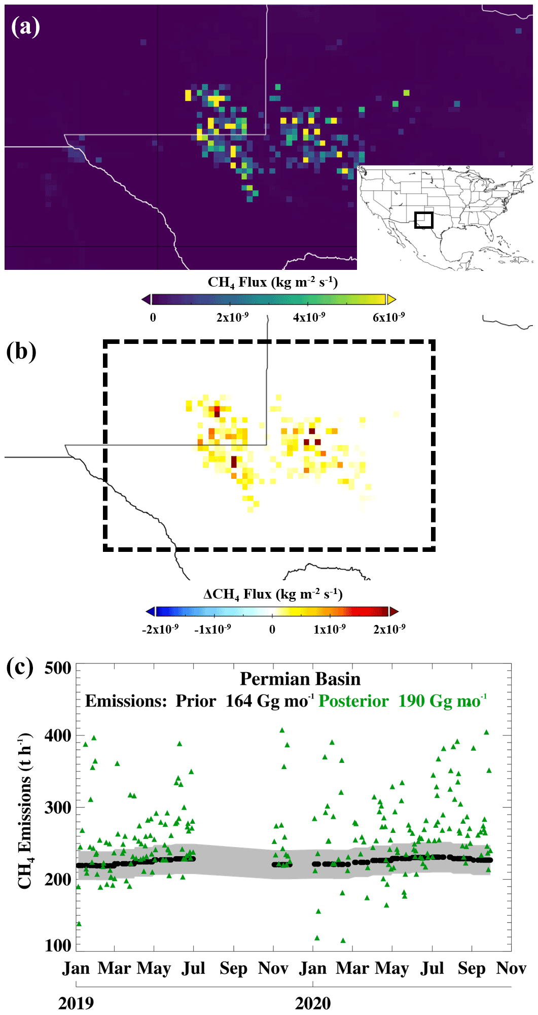
Figure 3 (a) Average prior Permian Basin CH₄ emissions for 2019. (b)  Average of posterior minus prior anthropogenic CH₄ emissions over the Permian Basin for January–June 2019, excluding days for which observations were not available. (c) Time series of total prior (black circles) and posterior (green triangles) anthropogenic CH₄ emission estimates within the $\mathrm{6}{}^{\circ }\times \mathrm{4}{}^{\circ }$ Permian Basin domain, centred around 32^∘ N, 103^∘ W (black box in b) for 2019–2020, excluding days for which observations were not available. The shaded error denotes prior uncertainty.

During the 2020 slowdown Lyon et al. (2021) derived tower and aircraft based CH₄ emission estimates from the Permian Basin. They found that emissions from January to March 2020 (134±12 Gg per month) reduced during the onset of the slowdown (April: 47±10 Gg per month) and subsequently increased again as oil price partially recovered in June (107±13 Gg per month). For the same period, we find only a small decrease in emissions from January to March averages (188±45 Gg per month) to April (183±34 Gg per month). This decreasing trend continues into June (178±14 Gg per month). However, we find that between July and September emissions noticeably increase to 215±40 Gg per month, suggesting that the rebound found by Lyon et al. (2021) might be detected, in our system, from July onwards. The difference in magnitude of emissions between the two studies is, in part, a result of the different domains used.

3.3.2 Regional emissions – Bakken Formation, USA and Canada

The Bakken Formation, predominantly in North Dakota, is a major oil-producing region within both the USA and Canada. The rig count in the region has declined in recent years; however, except for during the initial 2020 global slowdown, both oil and gas production have seen large increases in the past decade (EIA, 2021). During recent years various management methods have sought to reduce fugitive emissions from the region; however, it remains one of the largest emitting regions within North America (Schneising et al., 2020).

A previous study estimated average CH₄ emissions from the Bakken Formation between 2018 and 2019 of 74±47 Gg per month (Schneising et al., 2020). These were estimated using a Gaussian integral method and TROPOMI data. Our prior emissions (87 Gg per month) for a $\mathrm{1}{}^{\circ }\times \mathrm{1}{}^{\circ }$ domain centred around 48.5^∘ N, 103^∘ W for 2019 are larger than those previously derived estimates. Our posterior results for 2019 (77±42 Gg per month) show large variability, but an overall positive growth in emissions from the region (Fig. 4). These estimates agree with those derived by Schneising et al. (2020). For 2020, a period not included in their study, we find larger average emissions relative to 2019 (86±52 Gg per month). Unlike the Permian Basin example, the agreement found here is based upon two different top-down approaches, our 4D-Var IFS system and the Gaussian integral method of Schneising et al. (2020).

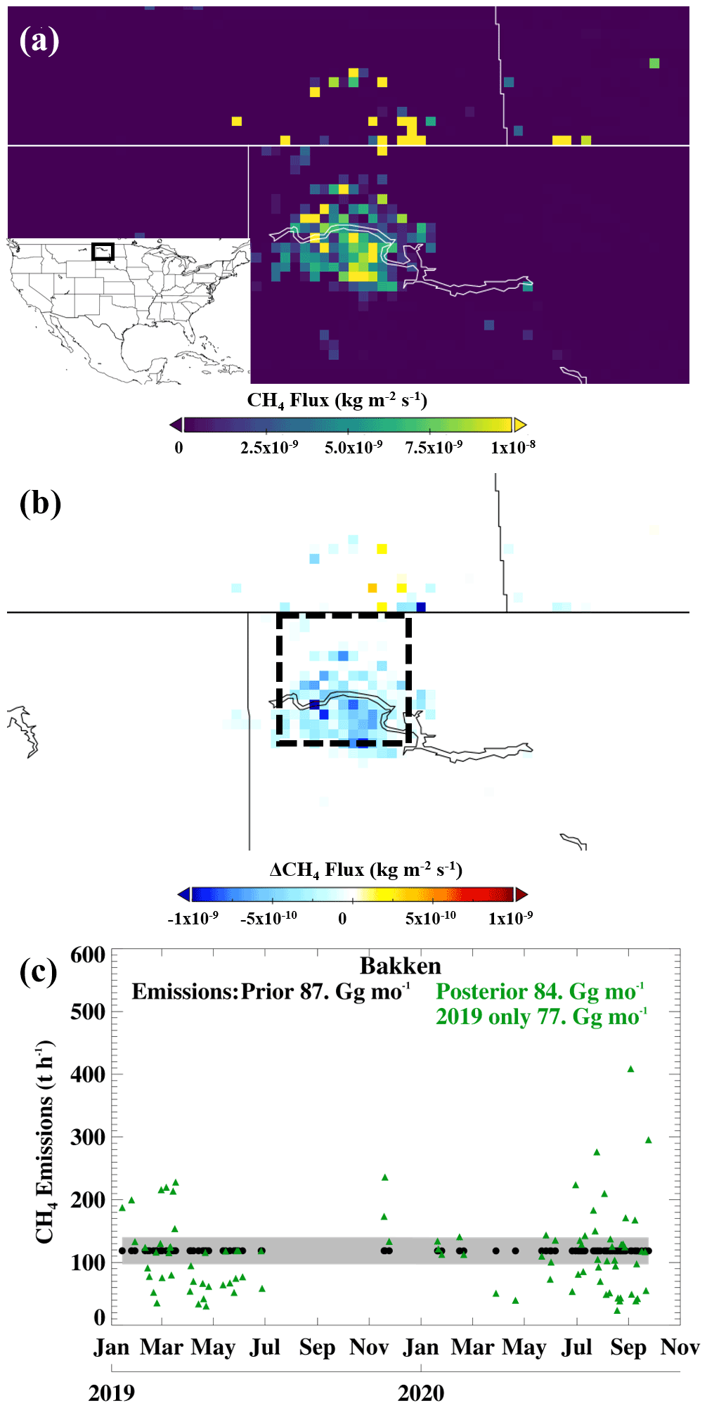
Figure 4 (a) Average prior Bakken CH₄ emissions for 2019. (b) Average of posterior minus prior anthropogenic CH₄ emissions over Bakken for January–June 2019, excluding days for which observations were not available. (c) Time series of total prior (black circles) and posterior (green triangles) anthropogenic CH₄ emission estimates within the $\mathrm{1}{}^{\circ }\times \mathrm{1}{}^{\circ }$ Bakken domain, centred around 48.5^∘ N, 103^∘ W (black box in b) for 2019–2020, excluding days for which observations were not available. The shaded error denotes prior uncertainty.

A possible CH₄ emission event is observed on the 4 September 2020 where emissions were estimated to increase by 350 % from a 2020 average of 120 to 410 t h⁻¹, which over the 24-h period equates to an additional 7 Gg CH₄. The source of this previously undocumented event is not clear – an incident reported at The Steelman Gas Plant in Saskatchewan, Canada (ID 48996) is a possibility; however, accurate attribution requires further investigation (Saskatchewan.ca, 2021). Several similar events of slightly smaller magnitude are also observed, the causes of which require further investigation.

3.3.3 Regional natural emissions – Lake Chad, Central Africa

The hydrology of Lake Chad and the surrounding area has recently undergone substantial variability on timescales ranging from seasonal to decadal (Pham-Duc et al., 2020), which is expected to have impacted both natural and anthropogenic emissions in the region. A recent study, using a similar prior to the one used here, performed a top-down inversion over tropical Africa using GEOS-Chem and GOSAT observations and found that posterior emissions increased relative to their prior over Lake Chad between 2016 and 2018, although these are not quantified (Fig. 3c of Lunt et al., 2019). Our results for 2019 and 2020 for a $\mathrm{1}{}^{\circ }\times \mathrm{1}{}^{\circ }$ box centred around the lake (13.0^∘ N, 14.3^∘ E) show posterior emissions (32±4 Gg per month) are 11 % higher than prior emissions (29±2 Gg per month) (Fig. 5). Observations are only available over the region for 65 out of 485 d, making estimations of the seasonal shift between the posterior and prior difficult. We are unable to attribute the increased emissions to a specific sector; however, based on prior information, it is likely to be from agricultural livestock or wetland sources. If this region-wide increment is the result of wetland emissions, with further refinement and accurate characterisation of prior error correlations, our system could be used to quantify emissions over wetland regions. Detailed comparison with Lunt et al. (2019) is not performed as the studies cover a different period and a thorough comparison requires further refinement of how natural emissions are treated in the prior. Here, we only note that the sign of the bias in both studies is the same and requires further investigation.

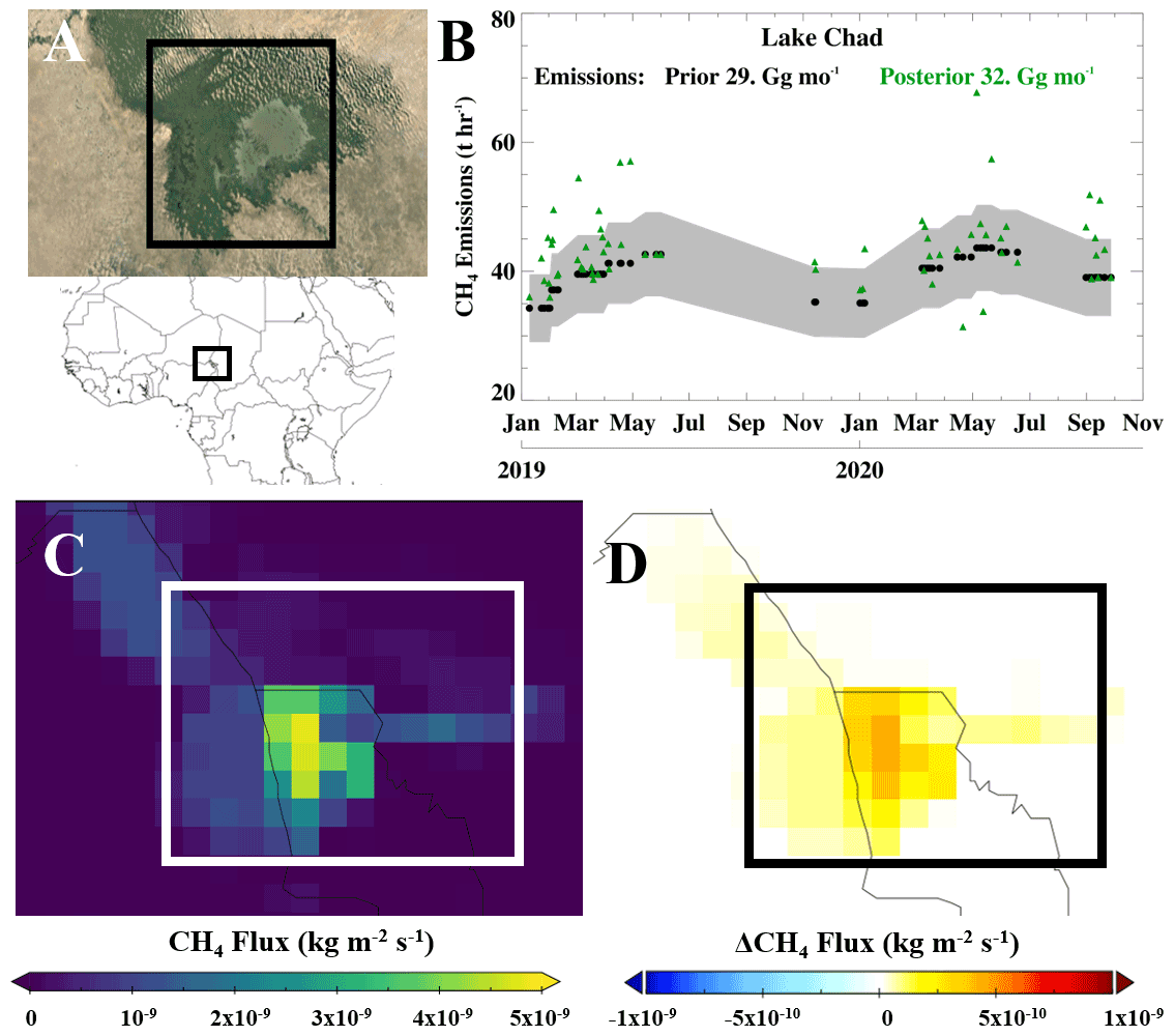
Figure 5 (a) The Lake Chad domain indicated by the black box (© Google Maps, 2021). (b) Time series of total prior (black circles) and posterior (green triangles) CH₄ emission estimates within the $\mathrm{1}{}^{\circ }\times \mathrm{1}{}^{\circ }$ domain, centred around 13.0^∘ N, 14.3^∘ E for 2019–2020, excluding days for which observations were not available. The shaded error denotes prior uncertainty. (c) Average prior CH₄ emissions for 2019. (d) Average posterior minus prior CH₄ emissions for January–June 2019, excluding days for which observations were not available.

3.3.4 Point source emissions – Appin colliery, Australia

The Appin colliery (34.2^∘ S, 150.8^∘ E), in New South Wales, Australia is an underground coal mine previously noted for having high CH₄ emissions (Varon et al., 2020). It represents a single point source, which is challenging to quantify as there are several nearby emission sources, including landfills, dairy facilities, and a gas-processing plant. Varon et al. (2020) used the high-resolution GHGSat-D instrument and integrated mass enhancement (IME) and cross-sectional flux (CSF) methods calibrated with large eddy simulations to derive vent emissions from the mine between 2016 and 2018. They estimated mean CH₄ emissions of 4.2 Gg per month (IME) and 3.6 Gg per month (CSF), lower than the prior used here (4.9±0.1 Gg per month, fugitive only: 4.3±0.1 Gg per month). We derived 2019–2020 average grid cell emissions of 4.6±0.5 Gg per month. Assuming little or no change in emissions between their 2016–2018 study period and our 2019–2020 estimate, our derived fugitive-only emissions (4.1±0.5 Gg per month) agree well with their findings (Fig. 6). For 2019, a business-as-usual year, which is nearer to the time period investigated in their study, fugitive emissions are even lower (3.9±0.5 Gg per month). These results suggest that our inversion might be capable of detecting biases in the prior from point sources, given sufficient observations ($\mathrm{100}/\mathrm{485}$ d observed), a relatively large point source ($>\sim \mathrm{4}$ Gg per month) and a suitable prior uncertainty estimate. Prior emission estimates appear to be in better agreement with our posterior in 2020, suggesting an increase in emissions, most likely from the colliery given that it is the dominant source in the region.

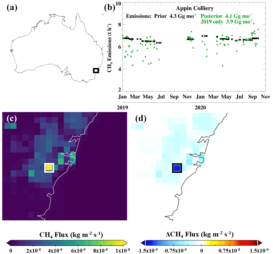
Figure 6 (a) A map of Australia with the Appin colliery domain indicated by the black box. (b) Time series of prior (black circles) and posterior (green triangles) fugitive CH₄ emission estimates within the domain for 2019–2020, excluding days for which observations were not available. (c) Average prior CH₄ emissions for 2019, the white box denotes the grid cell used to estimate emissions. (d) Average posterior minus prior CH₄ emissions for January–June 2019, excluding days for which observations were not available.

3.4 Emission estimates for temporary and shifting sources

The following four cases assess the quantification of emissions from specific release events, step changes in emissions or short-term observation periods, using documented examples and previously unexplored sources. As with the regional comparisons in the previous section, evaluation of the system is performed against multiple emission estimation systems beyond the 4D-Var approach used here.

3.4.1 Feasibility of estimating blow-out emissions – Eagle Ford blowout, USA (November 2019)

On 1 November 2019, a blowout event occurred at a gas well in the Eagle Ford Shale in Texas (28.9^∘ N, 97.6^∘ W), which was followed by a diminishing 20-d release event (Cusworth et al., 2021). Cusworth et al. (2021) estimated emissions of the blowout using several estimation techniques, including the Integrated Methane Enhancement algorithm (Varon et al., 2018), and multiple observation platforms, including TROPOMI. Observations directly over the blowout were made from TROPOMI on 2, 3, 15 and 18 November 2019. We further extended our analysis to all observations made between 15 October and 28 November 2019 within $\mathrm{2}{}^{\circ }\times \mathrm{2}{}^{\circ }$ domain centred around the blowout (Fig. 7). We found that when blowout emissions peaked on 1/2 November 2019, posterior emissions at the site were ∼40 % higher than prior emissions; however, the magnitude of the posterior emissions (2.5 t h⁻¹) is noticeably lower than the 28–61 t h⁻¹ previously estimated (Cusworth et al., 2021). As expected, posterior emission estimates return to near prior levels after the initial blowout (Fig. 7c–e). Estimates provided by Cusworth et al. (2021) would require more than a 1500 % increase in emissions relative to our prior, which is unlikely to be achieved with our relatively modest prior error (87 %). It is likely given the model resolution and prior information that posterior emissions are incorrectly attributed to nearby grid cells. This is evident in the mapped scaling factors, which show increases incorrectly applied slightly to the west of the blowout location. Within a $\mathrm{4}{}^{\circ }\times \mathrm{4}{}^{\circ }$ domain surrounding the blowout site posterior and prior emissions typically agree well for months excluding November, suggesting that any differences occurring in November could be attributed to the well blowout. Based on this assumption we used the residual from the posterior minus the prior to estimate blowout emissions on 2 November 2019 of 140 t h⁻¹, which is more than double the estimate of Cusworth et al. (2021). These results suggest that the system, as presented here, can detect such events but cannot accurately quantify a well blowout of this magnitude over an oil field. It could however be used as a crude quantification of emissions from such a blowout over a larger domain, assuming other sources are well known. A more accurate quantification of emissions from release events of this nature, requires further development and possibly the implementation of alternative techniques well adapted for missing sources (e.g. Yu et al., 2021).

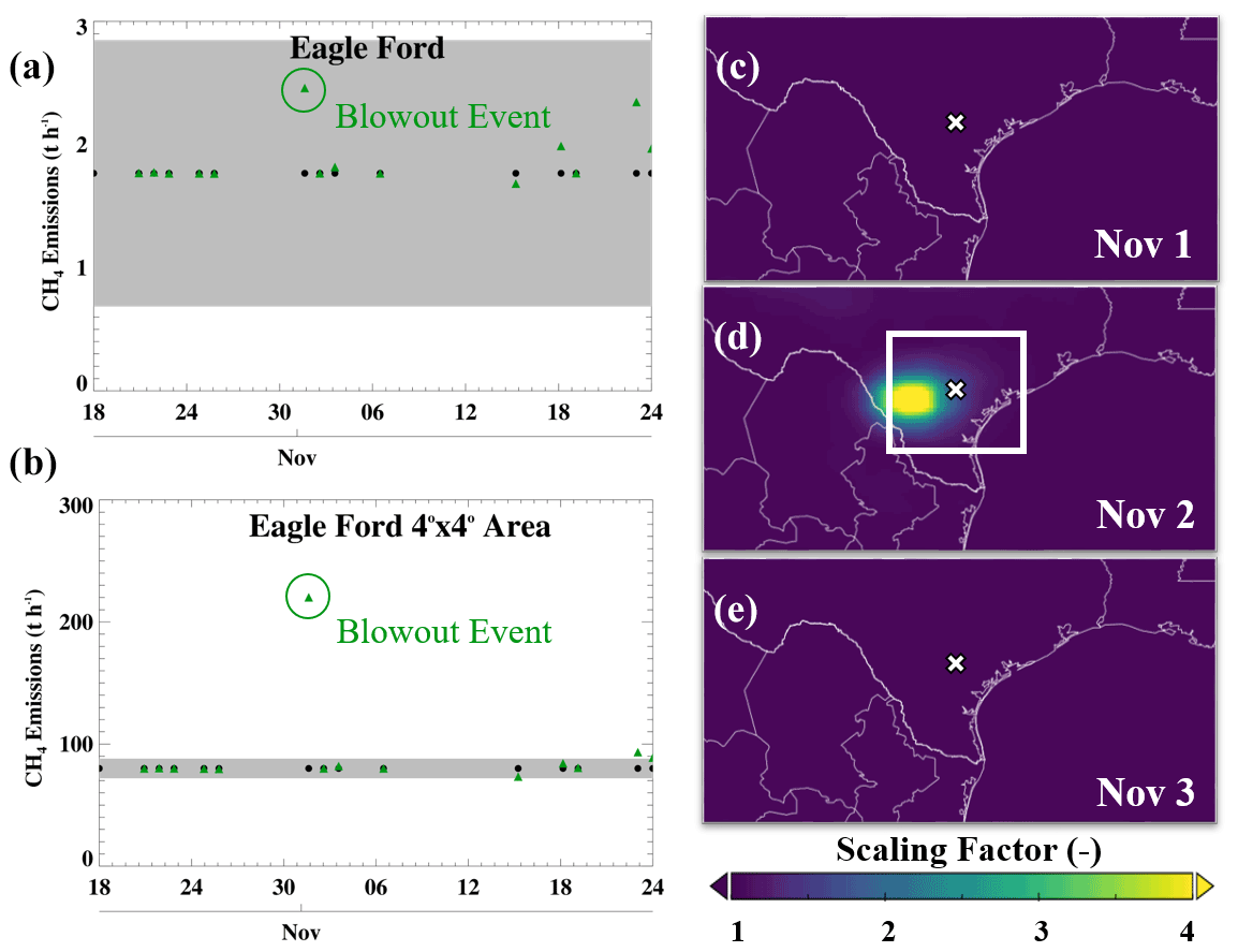
Figure 7 Prior (black circles) and posterior (green triangles) anthropogenic CH₄ emission estimates, where observations are available, over an oil well blowout event in Eagle Ford, USA, during October/November 2019 at the grid scale (a) and within a $\mathrm{4}{}^{\circ }\times \mathrm{4}{}^{\circ }$ domain (b). The shaded error denotes prior uncertainty. The nearest date (2 November) to the event, which occurred on 1 November, is also indicated. Regional scaling factor values from the inversion for 1 November (c), 2 (d) and 3 (e). Eagle Ford blowout site marked with an “x” and $\mathrm{4}{}^{\circ }\times \mathrm{4}{}^{\circ }$ domain denoted.

3.4.2 Feasibility of 1-d emission estimates – Upper Silesian Coal Basin, Poland (June 2018)

The Upper Silesian Coal Basin (USCB) is one of the largest CH₄- emitting regions in Europe, with emissions originating from ∼40 coal mines (EEA, 2021). The region extends from southern Poland across the border to Czechia, where CH₄ is released from deep coal deposits and emitted to the atmosphere via ventilation shafts (Fiehn et al., 2020).

To evaluate the feasibility of the system to quantify regional CH₄ emission sources within a 24-h window we performed a 1-d inversion over the USCB. Results were compared with emission estimates derived using aircraft observations combined with Eulerian and Lagrangian dispersion models (Kostinek et al., 2021) and a mass balance approach (Fiehn et al., 2020). These studies used extensive flight data from 6 June 2018 to derive regional CH₄ emission estimates of 35–40 Gg per month. The CoMet v2 bottom-up inventory (Fiehn et al., 2020) was specifically compiled for the purpose of the flight campaign and estimated emissions in the region of 48 Gg per month. Our results for 6 June 2018 estimated USCB emissions of 48 Gg per month, compared with our prior estimate of 53 Gg per month (Fig. 8). This shows good agreement with CoMet v2 and an improved agreement with the top-down estimates. From January–June 2019, posterior estimates (49±14 Gg per month) remain low relative to the prior; however, they increase in 2020, resulting in an average estimate for 2019–2020 of 52±16 Gg per month compared with a prior of 53±1 Gg per month. This suggests that although emissions in the basin increased over the simulation duration, they might have been consistently overestimated in the prior. The prior emissions do not consider daily variability, whereas considerable variability was estimated by the posterior (1.7±0.5 Gg d⁻¹).

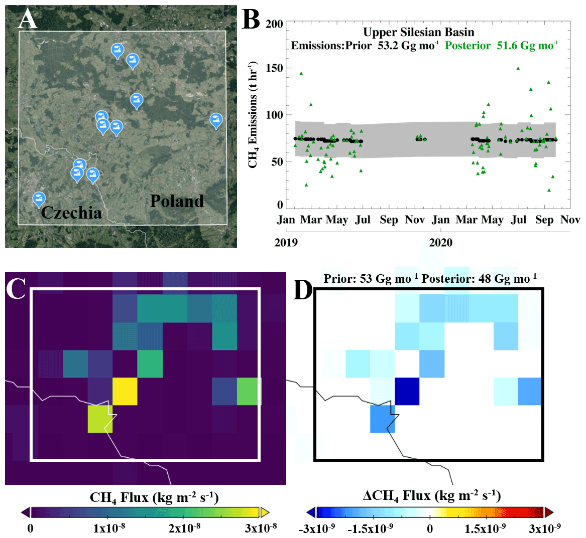
Figure 8 (a) The Upper Silesian Coal Basin $\mathrm{1}{}^{\circ }\times \mathrm{0.5}{}^{\circ }$ domain indicated by the white box, centred around 50.0^∘ N, 18.7^∘ E. Also shown are 11 major coal mines in the region (© Google Maps, 2021). (b) Time series of total prior (black circles) and posterior (green triangles) CH₄ emission estimates within the domain for 2019–2020, where observations and inverse simulations were available. The shaded error denotes prior uncertainty. (c) Prior total CH₄ emissions for 6 June 2018. (d) Average posterior minus prior CH₄ emissions for 6 June 2018.

3.4.3 Detection limit of inversion system – oil fields, Algeria (2019–2020)

The CH₄ emissions from a point source release event from a well pad at the Hassi Messaoud oil field in Algeria (31.7^∘ N, 5.9^∘ E) from October 2019 until August 2020 were previously quantified (Varon et al., 2021). Using Sentinel-2 observations they derived mean emissions of 6.7±4.0 Gg per month. From our inversions, and using only dates where TROPOMI observations were available within 0.4^∘ of where the leak occurred (21 d between 9 October 2019 and 9 August 2020), we found average CH₄ emissions within a $\mathrm{1}{}^{\circ }\times \mathrm{1}{}^{\circ }$ domain of 17.6±2.7 Gg per month (Fig. 9b). After the leak was sealed average emissions decreased to 15.3±2.6 Gg per month. Assuming any difference in emissions between the two time periods was caused by the release event, we estimate mean leak emissions of 2.4±0.6 Gg per month. This suggests that some detection might have been made, but quantification was not accurate when compared with a previous study (Varon et al., 2021). It seems likely that the magnitude of the leak (<4 Gg per month) approaches the detection limit of the inversion performed here, and far exceeds the limit for accurate quantification. Additionally, the low number of observation days during the 10-month leak period (21 d), might have contributed to the lack of robust detection.

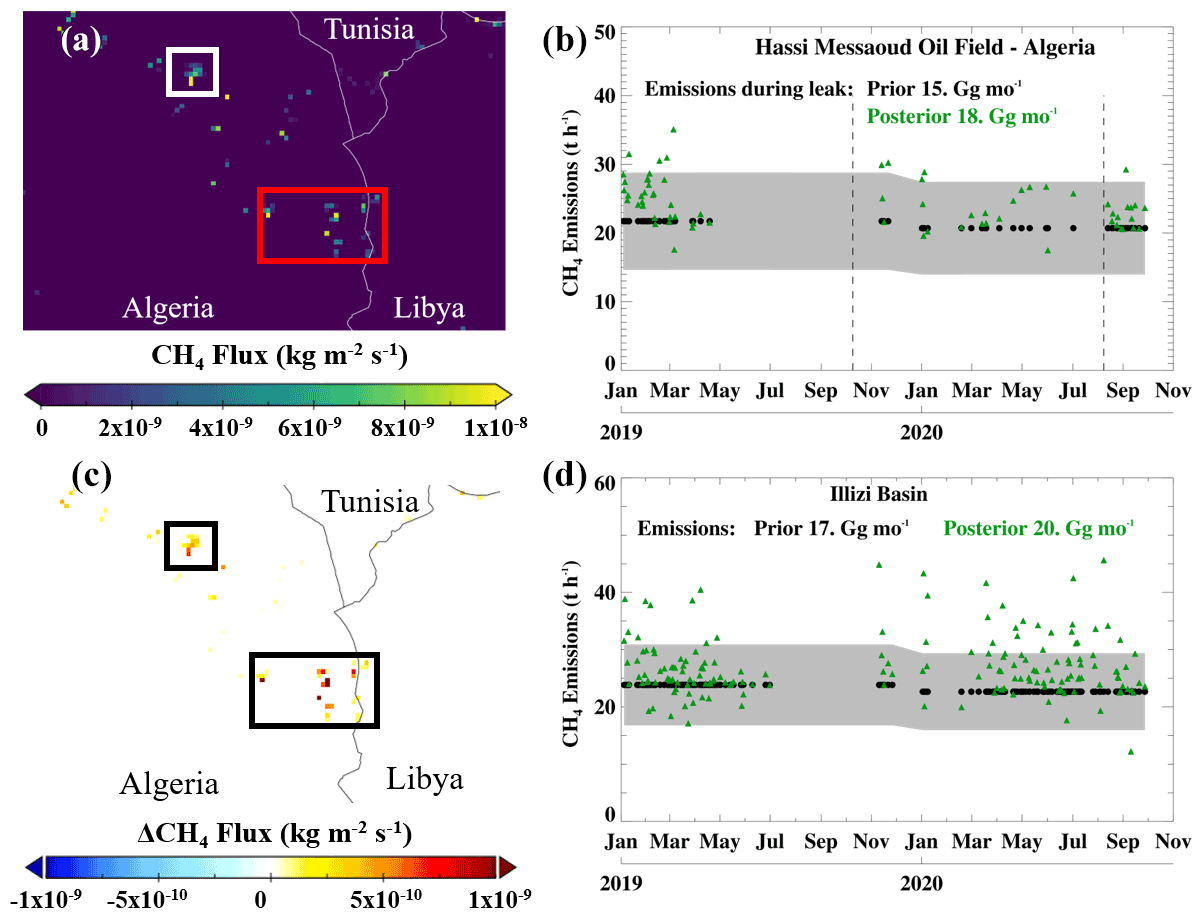
Figure 9 (a) Prior average anthropogenic CH₄ emissions for Eastern Algeria, 2019. The domains for the Hassi Massaoud oil field ($\mathrm{1}{}^{\circ }\times \mathrm{1}{}^{\circ }$, white box) and part of the Illizi Basin ($\mathrm{3}{}^{\circ }\times \mathrm{1.5}{}^{\circ }$, red box) are marked. Time series of total prior (black circles) and posterior (green triangles) CH₄ emission estimates within the Hassi Massaoud (b) and Illizi Basin (d) domains for 2019–2020, where observations and inverse simulations were available. The shaded error denotes prior uncertainty. (c) Average posterior minus prior CH₄ emissions for January–June 2019, using dates where nearby observations were available.

The Illizi Basin (28.3^∘ N, 9.0^∘ E) is one of the largest gas-producing regions in Algeria and is currently undergoing planned expansions (Ouki, 2019). Results from a $\mathrm{3}{}^{\circ }\times \mathrm{1.5}{}^{\circ }$ domain within the basin suggest that average emissions might be ∼20 % higher (20±3.9 Gg per month) than those estimated by the prior inventory (16.9±0.4 Gg per month) between 2019 and 2020 (Fig. 9d). These results suggest that the Illizi Basin might be a larger source of CH₄ emissions than the Hassi Messaoud oil field (17.5±2.5 Gg per month), although it should be noted that the domain area is larger. As with the Hassi Messaoud oil field, with our system, it is not possible to attribute the emission changes to a specific facility but rather to the entire region (∼200 km²).

3.4.4 Detection of unknown sources – Istanbul, Turkey (2020)

Istanbul is the most populous city in Europe, with prior CH₄ emission estimates of 56 Gg per month, making it one of the largest emitting regions of Europe. Prior information attributes 86 % of those emissions to the solid waste and wastewater sector. Inversion results from a $\mathrm{1}{}^{\circ }\times \mathrm{1}{}^{\circ }$ domain centred around Istanbul (41.0^∘ N, 29.0^∘ E) showed an unexpected increase in emissions from July 2020 onwards, before which posterior (56±9 Gg per month) emission estimates were in good agreement with the prior (57±3 Gg per month) (Fig. 10). From July to September 2020, these emissions increased by 42 % to 81±25 Gg per month. The reason for this step change in emissions is unclear and, assuming that the posterior estimates are robust, requires further investigation given the magnitude of the increase. Increased emissions are derived over a large area of the Istanbul domain; however, given the results from the Eagle Ford blowout region, it is possible that the estimated increase is from a point source. It is also unclear whether this is a new persistent emission source or if it only occurred over a period of several months.

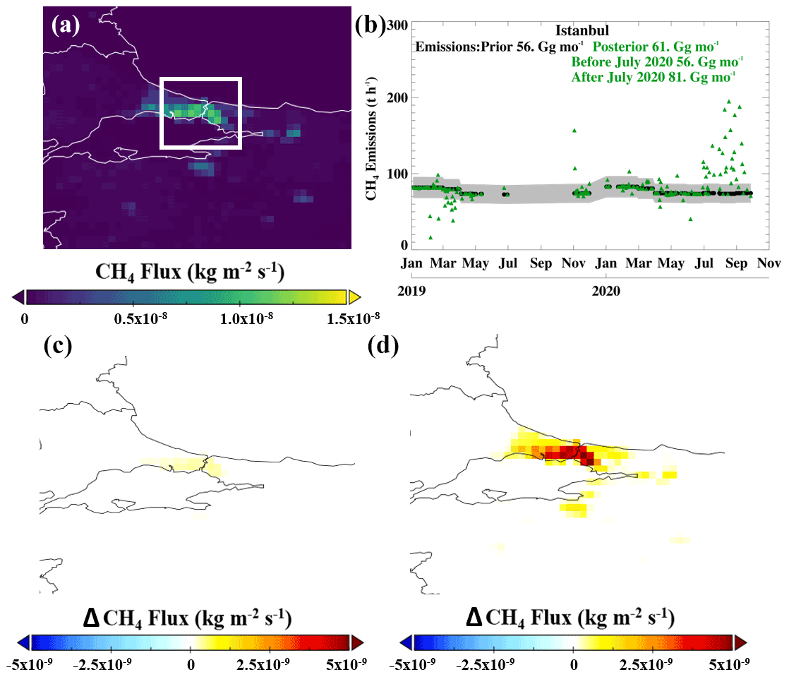
Figure 10 (a) Prior CH₄ emissions within the Istanbul domain for September 2020. (b) Time series of total prior (black circles) and posterior (green triangles) CH₄ emission estimates within the $\mathrm{1}{}^{\circ }\times \mathrm{1}{}^{\circ }$ domain, centred around 41^∘ N, 29^∘ E (white box in a) for 2019–2020, where observation and inverse simulations are available. The shaded error denotes prior uncertainty. Average posterior minus prior CH₄ emissions for May (c) and September (d) 2020, using dates where nearby observations were available.

3.5 CH₄ emissions during the COVID-19 period

To evaluate the impact on anthropogenic CH₄ emissions from the global slowdown, caused by the COVID-19 pandemic, we compared posterior emissions from January to June of 2019 and 2020. Globally, monthly average anthropogenic emissions for the 6-month period in 2020 (30.0 Tg ± 1.8 Tg per month) are found to be 1.6 % (470 Gg per month) higher than for 2019 (29.5±2.0 Gg per month) (Fig. 11). These increased emissions contributed to the observed increased atmospheric growth rate between 2019 (9.8±0.6 ppb yr⁻¹) and 2020 (15.6±0.4 ppb yr⁻¹) (NOAA, 2021). Sector-specific attribution shows that the energy ($+\mathrm{220}\pm \mathrm{130}$ Gg per month) and agriculture ($+\mathrm{160}\pm \mathrm{40}$ Gg per month) sectors are the largest contributors to this increase, with smaller contributions from the waste ($+\mathrm{50}\pm \mathrm{30}$ Gg per month) and other anthropogenic sources ($+\mathrm{30}\pm \mathrm{20}$ Gg per month).

Figure 11 Estimated national or regional average CH₄ emission change between 2020 and 2019 for January to June, derived using an IFS inversion for the largest emitters for (a) energy, (b) agriculture, (c) waste and (d) other anthropogenic sources. (e) Global change in sector-specific monthly CH₄ emissions for the same period. (f) National or regional change in total anthropogenic CH₄ emissions for the same period.

When compared with 2019, anthropogenic CH₄ emissions in 2020 were larger pre-slowdown (January–February: $+\mathrm{470}\pm \mathrm{0}$ Gg per month), considerably larger during the early stages of the slowdown (March–April: $+\mathrm{680}\pm \mathrm{80}$ Gg per month) and only slightly larger in the latter months of the initial slowdown (May–June: $+\mathrm{270}\pm \mathrm{30}$ Gg per month). Assuming that no other factors contributed to this observed difference in emissions between the two years, this suggests that, globally, the impact of the slowdown might have initially increased emissions and subsequently reduced them, although emissions for all 6 months were higher in 2020 than for 2019. This trend in emissions was mainly driven by energy sector emissions (January–February: +200 Gg per month, March–April: +390 Gg per month, May–June: +80 Gg per month), whereas the agricultural sector showed a relatively consistent increase, relative to 2019, for all months (+160 Gg per month).

When averaged over all 6 months, an increase in emissions between 2019 and 2020 was estimated in 6 out of 8 of the largest emitting regions, with the only exceptions being Pakistan (−0.6 Gg per month) and Brazil (−23 Gg per month). The largest increase was in China (+220 Gg per month), of which, over half originated from the energy sector, specifically from the northern coal mining regions. The difference in emissions from China, relative to 2019, was the main driver for the global trend, with increases pre-slowdown (January–February: +230 Gg per month), large increases during the initial slowdown (March–April: +300  Gg per month) and only small increases in the latter months (May–June: +120 Gg per month). As with the global signal, this monthly variability is attributed to changes in energy sector emissions. It should be noted that the slowdown in China occurred from the end of January and results show that, relative to 2019, 2020 emissions from China were noticeable larger in January (+270 Gg per month) and only slightly larger in February (+190 Gg per month) suggesting a brief impact from the slowdown.

For the first 6 months emissions for 2020 from India were on average 65 Gg per month higher than for 2019, with noticeable large increases in emissions from the agricultural sector in June 2020 (+110 Gg per month), which contributed to almost half of the global increase for June. The increased emissions in June mainly originated from the Uttar Pradesh region in north India. Similar increases in agricultural emissions are found over Bangladesh for June (+110 Gg per month). Poor prior information in the region may have resulted in the misallocation of emissions, which could have originated from the large Baghjan Oil Field blowout in Assam, India, in May/June 2020. Energy sector emissions from Indonesia were consistently higher in 2020 (+13 to +46 Gg per month) and relatively unchanged for the remaining regions ($<\pm \mathrm{25}$ Gg per month).

Given the limitations of our system we have typically focused on anthropogenic emissions; however, natural fluxes were also derived. Global posterior results for the first half of 2020 show a reduction in both wetland (−36 Gg per month) and fire (−150 Gg per month) emissions when compared with 2019, with large monthly variability. The total global decrease in fire emissions is unchanged from the estimated prior emissions, taken from GFAS, which is based on satellite observations. The wetland emission change originates from South America, mainly from Brazil (−10 Gg per month) and Argentina (−28 Gg per month). These reduced emissions were likely caused by large-scale droughts, which occurred in early 2020 (Marengo et al., 2021). Although the months simulated are not typically associated with the boreal northern hemisphere fire season, most of the reduction in biomass- burning emissions came from Russia (−110 Gg per month) and Canada (−44 Gg per month). This change was caused by a particularly active arctic fire season in 2019 (Zhang et al., 2021) and large wildfires in northern Alberta in May 2019. Relative to 2019, increased fire emissions from Australia are derived for January 2020 (+220 Gg per month). It is estimated that an unusually intense bushfire season (Shiraishi and Hirata, 2021) resulted in the release of 330 Gg CH₄ from Australia over the month of January alone. More specifically, the emissions were unusually large from New South Wales and Victoria.

A limitation of the current system is the use of a climatological OH sink, which is the primary oxidant for atmospheric CH₄. Currently, OH is not included in the control vector and does not respond to changes in atmospheric chemistry. Formation pathways of OH are influenced by atmospheric NO_x concentrations, which were estimated to have decreased during the slowdown period (Doumbia et al., 2021). Several simulations were performed using multiple chemistry schemes to assess the atmospheric impact of OH when using a slowdown-adjusted emission scenario (Huijnen et al., 2021). Results show global OH decreases of 1–3 % during the slowdown period; however, a heterogenous spatial pattern is observed near the surface with increased OH concentrations over some regions. This would suggest that the 2020 increased emissions found here might be overestimated; however, the derived emission increases in January and February of 2020, relative to 2019, are unlikely to have been influenced by OH changes caused by the global slowdown. Future developments will include the inversion of NO_x emissions during the global slowdown and their effect on OH concentrations, resulting in more accurate source-sink attribution.

4 Conclusions

We have investigated the feasibility of monitoring CH₄ emissions using a global online high-resolution (∼80 km), short-window 4D-Var (24 h) data assimilation system and satellite observations from multiple sensors. This system optimises both the initial 3D atmospheric concentration of CH₄ and surface fluxes, whilst implicitly accounting for transport errors associated with uncertainty in meteorological initial conditions. The prior emission errors were selected based on comparisons with independent TCCON retrievals. We identify strengths and weaknesses of our inversion system by performing case study comparisons with other well-established flux estimation systems at a range of spatiotemporal scales.

Globally, a small decrease in annual CH₄ emissions, relative to the prior, is estimated by the inversion for 2019 (∼1 %). On a national scale, we found decreased anthropogenic emissions from China (−5 %) and India (−3 %), with small increases from the USA (+0.5 %) and Brazil (+1.3 %) contributing to this change. This is in general agreement with a recent inverse study (Qu et al., 2021).

To evaluate the system on the regional and point scale, several anthropogenic case studies were selected (Table 1). Posterior estimates of anthropogenic sources with persistent emissions typically showed good agreement with previous studies. In addition, the posterior quantification of emissions from a large biogenic source region, Lake Chad, compared well with a previous inversion study (Lunt et al., 2019).

We investigated the feasibility of quantifying emissions at a high spatial, temporal and spatiotemporal resolution. Emissions from a well leak in the Hassi Messaoud oil field, which persisted for several months, were found to be at or around the detection limit of the system (∼9 t CH₄ h⁻¹) and beyond the limit for accurate quantification. Similarly, emissions from a large well blowout in Eagle Ford were found to be misallocated to the surrounding region owing to poor prior information and too coarse a model resolution. In contrast, inverse estimates from a known persistent point source, the Appin Mine, were found to be in good agreement with a previous top-down estimate (Varon et al., 2020). For a 1-d period over a large region, the Upper Silesian Basin, inverse estimates agreed well with previous studies (Fiehn et al., 2020; Kostinek et al., 2021). Overall, these case studies suggest that our inverse system might be suitable for regional-scale (∼100 km²) emission quantification over a short time-period (24 h), given that sufficient satellite observations are available. Given adequate prior information our system is also capable of quantifying emissions from a persistent point source (e.g. Appin Mine, Australia).

Several previously undocumented CH₄ emission sources were also investigated, including an unknown release event from the Bakken Formation. Prior emission estimates were persistently found to be underestimated by ∼20 % from the Illizi Basin between 2019 and 2020, possibly owing to an expansion in operations. Finally, a noticeable step change in emissions from Istanbul was observed from July 2020, when emissions increased by ∼40 %, the reason for which is unknown and would require further investigation.

The impact on CH₄ emissions from the global slowdown in response to COVID-19 was investigated using inversions from the first half of 2019 and 2020. The slowdown coincided with a year where CH₄ growth (15.6 ppb) was the largest since records began in the early 1980s. We found in the early part of 2020 that atmospheric growth was, in part, driven by anthropogenic emissions that were larger than for 2019 (January to February: $+\mathrm{470}\pm \mathrm{0.0}$ Gg per month). These emissions further increased during the early stages of the slowdown (March to April: $+\mathrm{680}\pm \mathrm{80}$ Gg per month), almost half of which originated from the energy sector in China. Had this been a sustained increase, the global growth rate for 2020 would have been even larger. However, during the later months of the slowdown period emissions reduced, although they were still slightly higher than 2019 values (May to June: $+\mathrm{270}\pm \mathrm{30}$ Gg per month). Assuming no other contributing factors, this suggests that the slowdown might have acted to reduce emissions, mainly from the energy sector. By using the relative differences for January and February as a reference for the long-term growth between 2020 and 2019 and assuming business-as-usual for those months, we conclude that the overall impact of the global slowdown on CH₄ emissions is small. The slowdown in China occurred at the end of January; using the aforementioned assumption but only for January results in the same conclusion of a minimal impact on emissions during the entire 6-month period from the slowdown. The increased atmospheric growth is found to be the result of a continued increasing trend in CH₄ emissions and possibly related to changes in atmospheric chemistry in response to the slowdown (e.g. Stevenson et al., 2021). The reason for the observed monthly variability in emissions is unclear; it is possible that a reduction in energy demand resulted in increased venting of natural gas or that a change in working practice led to an increase in fugitive emissions, which subsequently fell below previous levels after several months of reduced demand.

Future developments will be based on a hybrid-ensemble system that will extend the assimilation window and utilise observations of co-emitted species (e.g. NO₂, CO). Additionally, improved representation of biogenic fluxes as well as spatiotemporal correlations in the prior will provide more accurate posterior estimates and uncertainties. Finally, the current lack of error propagation across the 4D-Var windows, will be addressed in an upcoming version of the system and more dynamical approaches to automatically adjusting inaccurate prior information will be implemented to better constrain missing and intermittent sources. These improvements will allow for constraints of other greenhouse gas emissions, most notably CO₂.