Interannual variability of terpenoid emissions in an alpine city

Terpenoid emissions above urban areas are a complex mix of biogenic and anthropogenic emission sources. In line with previous studies we found that summertime terpenoid fluxes in an alpine city were dominated by biogenic sources. Inter-seasonal emission measurements revealed consistency for monoterpenes and sesquiterpenes but a large difference in isoprene between the summers of 2015 and 2018. Standardized emission potentials for monoterpenes and sesquiterpenes were 0.12 nmol m⁻² s⁻¹ and $\mathrm{3.0}\times {\mathrm{10}}^{-\mathrm{3}}$ nmol m⁻² s⁻¹ in 2015 and 0.11 nmol m⁻² s⁻¹ and $\mathrm{3.4}\times {\mathrm{10}}^{-\mathrm{3}}$ nmol m⁻² s⁻¹ in 2018, respectively. Observed isoprene fluxes were almost 3 times higher in 2018 than in 2015. This factor decreased to 2.3 after standardizing isoprene fluxes to 30 ^∘C air temperature and photosynthetic active radiation (PAR) to 1000 µmol m⁻² s⁻¹. Based on emission model parameterizations, increased leaf temperatures can explain some of these differences, but standardized isoprene emission potentials remained higher in 2018 when a heat wave persisted. These data suggest a higher variability of interannual isoprene fluxes than for other terpenes. Potential reasons for the observed differences such as emission parameterization, footprint changes, water stress conditions, and tree trimming are investigated.

1 Introduction

Biogenic and anthropogenic volatile organic compounds (BVOCs, AVOCs) in the atmosphere can contribute to surface air pollution due to both their influence on tropospheric ozone formation and their potential to act as precursors for secondary organic aerosol (Derwent et al., 1996; Fehsenfeld et al., 1992; Fuentes et al., 2000; Goldstein et al., 2009; Laothawornkitkul et al., 2009; Riipinen et al., 2012). BVOCs play a particularly important role globally, as their emission strength is estimated to be 10 times larger than AVOCs (Guenther et al., 2012; Piccot et al., 1992). Also, many BVOCs are characterized as highly reactive (Atkinson and Arey, 2003; Fuentes et al., 2000), resulting in rapid peroxy radical chemistry important for ozone and ultrafine particle formation processes (Simon et al., 2020). Of the total global BVOC emissions, terpenes dominate, with 50 % attributed to isoprene, 15 % to monoterpenes, and about 0.5 % to sesquiterpenes (Guenther et al., 2012). In predominantly isoprene-emitting forests isoprene was found to be responsible for 50 %–100 % of the tropospheric ozone production (Duene et al., 2002; Tsigaridis and Kanakidou, 2002; Poisson et al., 2001). In coniferous forests monoterpene and sesquiterpene emissions often dominate (Johansson and Janson, 1993; Thunis and Cuvelier, 2000; Juráň et al., 2017). It has been shown that RO₂ self-reactions of monoterpenes and sesquiterpenes can rapidly create highly oxidized matter (HOM) and are a key player for new particle formation (NPF) events in forests under low NO_x conditions (Simon et al., 2020).

In urban environments where the mixture of BVOCs and AVOCs is more complex, several recent studies point out the importance of biogenic emissions for local air quality (Simon et al., 2019, Bonn et al., 2018; Churkina et al., 2017; Ren et al., 2017; Papiez et al., 2009; Chameides et al., 1988) and that the BVOC influence is especially high during summertime heat waves (Churkina et al., 2017).

Particularly in summer, biogenic sources dominate in urban environments. For example, Yadav et al. (2019) found an increased importance of biogenic isoprene in an urban site in western India during the pre-monsoon season when temperatures and PAR were high, and Hellen et al. (2012) found a strong biogenic influence on isoprene and monoterpene concentrations in Helsinki in July. Summertime isoprene in two large Greek cities was determined by positive matrix factorization (PMF) to mainly (60 %–70 %) originate from vegetation (Kaltsonoudis et al., 2016). Yang et al. (2005) showed a strong seasonal and daily cycle in isoprene, therefore attributing it to biogenic sources in an urban region in Taiwan. Borbon et al. (2002) showed that biogenic sources strongly superimpose the traffic emissions of isoprene in summer in an urban area in France. Wagner and Kuttler (2014) found that during summer afternoons in an urban area in Germany anthropogenic influences on isoprene concentrations were negligible. Chang et al. (2014) and Wang et al. (2013) showed that in a tropical–subtropical metropolis biogenic contributions overwhelmed anthropogenic contributions of isoprene in summer and that biogenic sources started to dominate in all seasons above a threshold temperature of 17–21 ^∘C. Whereas all the studies cited above were based on concentration measurements for which the influence can be both local and regional as well as strongly modulated by atmospheric dilution, the following studies were based on eddy covariance flux tower sites. At temperatures over 25 ^∘C more than 50 % of the isoprene flux was found to be biogenic in origin in London with a mean daytime flux of 0.18 mg m⁻² h⁻¹ (Langford et al., 2010). Similarly, Valach et al. (2015) in a different study in London found a mean daytime flux of 0.2 mg m⁻² h⁻¹. Kota et al. (2014) found a daytime median flux of 2.1 mg m⁻² h⁻¹ over Houston, Texas, and attributed it to mostly biogenic sources. Park et al. (2010) also found in Houston, Texas, a daytime isoprene flux of 0.7 mg m⁻² h⁻¹. Rantala et al. (2016) found that 80 % of the measured 10 ng m⁻² s⁻¹ summer daytime isoprene flux near Helsinki could be attributed to biogenic sources by comparing emissions at low and high temperatures.

While there is evidence for urban trees having a positive influence on urban environments such as by mitigating the urban heat island effect, sequestering CO₂ and particles, and intercepting storm water (Escobedo et al., 2011; Connop et al., 2016; Livesley et al., 2016), BVOC emissions of urban trees and their subsequent effect on air pollution are very plant-species-dependent (Corchnoy et al., 1992; Steinbrecher et al., 2009; Fitzky et al., 2019) and should be taken into account when planting urban trees (Calfapietra et al., 2013; Churkina et al., 2015; Ren et al., 2017). Emerging evidence that isoprene-derived RO₂ competes with RO₂ radicals from higher-molecular-weight terpenes in the formation of new particles highlights the need to study emissions in different environments (Berndt et al., 2018).

Few studies characterize the interannual changes in BVOCs and even fewer such studies are available in urban environments. Vaughan et al. (2017) report airborne flux measurements over southern Sussex for two consecutive summers, showing different isoprene fluxes that can be explained by different temperature and cloud cover conditions. Warneke et al. (2010) tried to explain the measured interannual differences of a factor of 2 in fluxes of isoprene and monoterpene over Texas by temperature, drought effects, or influences from changes in leaf area index (LAI). Palmer et al. (2006) found a maximum of 20 %–30 % interannual difference in isoprene emissions using satellite-based isoprene quantification from formaldehyde measurements over North America. A model study by Steinbrecher et al. (2009) found only a 10 % annual difference in biogenic emissions from cold to hot years. Gulden et al. (2007) found that, on a regional scale, variations in leaf biomass density driven by variations in precipitation are, together with temperature and shortwave radiation variations, the most important factors for variations in BVOC emissions. Tawfik et al. (2012) found in a model study that interannual variation of isoprene emission is strongest in July with temperature and soil moisture explaining 80 % of the variations, whereas the influences of variations in photosynthetic active radiation (PAR) and LAI were negligible. In a 3-year study over a northern hardwood forest, Pressley et al. (2005) found that total cumulative isoprene fluxes varied only by 10 %.

Given the current lack of multiyear urban VOC flux measurements and our limited understanding of the interannual variability of biogenic and anthropogenic emission sources, the objective of the present study was to quantify the interannual variation of the urban ecosystem–atmosphere exchange of the three major isoprenoids, isoprene, monoterpenes, and sesquiterpenes, as well as to analyze the underlying drivers. We hypothesized (i) that the exchange of these BVOCs can be largely attributed to the spatiotemporal variability of biogenic sources and (ii) that differences in environmental forcings are the main drivers of interannual variability. To address these hypotheses, urban eddy covariance BVOC flux measurements during two growing seasons above the city of Innsbruck (Austria) are blended with bottom-up emission estimates based on a process-based model and a detailed urban tree inventory.

2 Materials and methods

2.1 Field site and instruments

VOC concentrations and flux measurements were conducted during two comparable summer periods (10 July–9 September 2015 and 27 July–2 September 2018) close to the city center of Innsbruck on the rooftop of one of the tallest buildings in the area. The data record in 2018 is continuous, and in 2015 the data record has a gap between 31 July and 3 August. Details on the Innsbruck Atmospheric Observatory (IAO) measurement site and instrument performance were published by Karl et al. (2018) and Striednig et al. (2020). Therefore, we give only a short summary of the study location and measurement details here. The measurement location (47^∘15^′51.66^′′ N, 11^∘23^′06.82^′′ E) is shown in Fig. 1a on a 2000×2000 m map surrounding the site. The dominant wind direction at the IAO is from the NE during the daytime and from the SW during nighttime (Karl et al., 2020; Striednig et al., 2020). Within 500 m from IAO, the mean building height is 17.3 m, whereas the model building height of about 19 m corresponds to the five- to seven-story buildings, which are more important in terms of their form drag. For this reason, the displacement height, zd, is estimated as 13.3 m (0.7 m × 19 m). The roughness length, z0, is 1.6 m.

Figure 1 (a) Map surrounding the Innsbruck Atmospheric Observatory (indicated with a red cross in the center) depicting trees, short vegetation, water, roads, paved areas, and buildings in dark green, light green, blue, white, light grey, and dark grey, respectively. Black dots represent individual trees from the city tree inventory. The study area is indicated with the red rectangle. The 2015 footprint density lines from 30 %–90 % are plotted as blue lines. (b) Same map as (a) with 2018 footprint density lines in black. (c) Diurnal cycle of average and standard error of PAR in 2015 (blue) and 2018 (black). (d) Diurnal cycle of average and standard error of ambient temperature in 2015 (blue) and 2018 (black). Maps were created in MATLAB (https://www.mathworks.com/, last access: 1 August 2021) and are based on OpenStreetMap (https://www.openstreetmap.org/copyright, last access: 1 August 2021) under the CC BY 3.0 AT license.

3D sonic wind, CO₂, and H₂O were measured with a CPEC200 (Campbell Scientific) eddy covariance system at a sampling frequency of 10 Hz on a tower on top of the building 42 m above street level. In 2015 the tower was at a provisional location at the north of the building; the heading direction of the sonic anemometer was 76^∘. Flow distortions for westerly winds due to the building and the support structure cannot be excluded. In the course of the establishment of the IAO lab the CPEC200 the inlets were moved ∼50 m to the southern edge of the building with an anemometer heading of 129^∘ and minimal flow disturbances. For comparability isoprenoid fluxes in this study are limited to the northeastern sector of [0^∘, 120^∘] in both years.

A heated inlet line led from the tower to a nearby laboratory hosting a PTR-QiTOF-MS instrument (IONICON Analytik, Sulzer et al., 2014), which allows for the acquisition of full, high-resolution, mass spectral information at 10 Hz. Residence time of air samples in the turbulently purged Teflon inlet line (Teflon PFA, $\mathrm{1}/\mathrm{4}$” ID x 12.7 m heated at 30 ^∘C) is about 0.4 s to keep wall loss and chemical transformation of isoprenoids negligible. Both summers the PTR-QiTOF-MS was operated in H₃O⁺ mode with standard drift tube conditions of 112 Townsend (E/N electric field strength). Regular instrument calibrations and zeroing revealed typical acetone and isoprene sensitivities of 1550 and 950 Hz ppbv⁻¹, respectively.

Incident PAR was calculated from shortwave radiation measured by a pyranometer (Schenk 8101, Schenk, Wien) by applying the relationship derived by Jacovides et al. (2003) (PAR $/$ shortwave radiation ∼0.46 during summer daytime conditions).

Precipitation data were collected 400 m south of our field site by a tipping bucket precipitation gauge (MPS TRWS 503) and a precipitation monitor (Thies 5.4103.10.000), mounted at 1.5 m above a grass surface, both operated by Zentralanstalt für Meteorologie und Geodynamik (ZAMG, Austrian Met-Service) at the station Innsbruck Universität (WMO SYNOP number 11320).

Due to the lack of directly measured city-scale soil moisture data, plant available soil moisture for 2015–2019 was retrieved as the SMAP level 4 3-hourly 9 km root zone soil moisture product (Reichle et al., 2018) via the AppEEARS interface (https://lpdaacsvc.cr.usgs.gov/appeears/, last access: 1 August 2021). Due to the large spatial footprint of this product, the corresponding data will only be used to interpret interannual differences in precipitation on soil moisture.

2.2 Eddy covariance fluxes

This study focuses on biogenic fluxes collected during summer 2015 and summer 2018. The presented eddy covariance flux measurements are used to constrain BVOC flux parameterizations. Biogenic emissions, in particular isoprene, are strongly light- and temperature-driven. As a consequence we selected daytime flux data. During daytime the flux footprint density points towards the east sector imposed by the local valley wind system. In order to test BVOC emission parameterizations we therefore selected daytime hours (06:00–18:00 local time) and mean wind directions from 0–120^∘. Data with wind direction from the south and exceeding a wind speed >10 m s⁻¹ were excluded as they can be attributed to foehn events, for which we believe current footprint density calculations bear too much uncertainty in an urban setting. Eddy covariance fluxes were calculated using a MATLAB^® code described by Striednig et al. (2020). Figure S1 shows the co-spectral response of the PTR-QiTOF-MS and inlet system. The loss of covariance of isoprenoid signals with vertical wind speed due to low-pass filtering is less than 4 % (see spectral analysis in the Supplement).

As QA $/$ QC criteria for fluxes we implemented a combination of steady-state filter of the respective scalar, the integral turbulence characteristics test of the wind components, and flow sector filtering, similar to the combination described in Chapter 4.2.5. in Foken (2008) with a required overall quality class of 6 or lower. According to Foken (2008), classes 1–6 can be used for long-term measurements of fluxes without limitations. Implementing these QA $/$ QC criteria reduced the available flux data by 29 % and 11 % in 2015 and 2018, respectively.

The footprint density representing the relative contributions of an air mass sample arriving at the flux tower was calculated following Kljun et al. (2015).

Regarding constraints on the lifetime of reactive terpenes, turbulent timescales (100 s) can be of the order of chemical timescales of some monoterpenes, which can react fast with ozone. We calculate the chemical loss by the following equation: $c\left(t\right)/c\mathrm{0}=\exp (-t_{\mathrm{turb}}/t_{\mathrm{chem}})$, where t_turb is the turbulent timescale and t_chem the chemical timescale. The turbulent timescale was obtained from the ratio of the measurement height (H) over the friction velocity ($H/u^{*}$). For typical turbulent timescales of 100 s, reaction with OH can be neglected.

Further, our analysis of emissions is primarily focused on the interpretation of daytime fluxes, when NO₃ radical chemistry plays a minor role compared to ozone. Ozone follows the expected diurnal cycle for an urban area (30–50 ppbv mixing ratios). Since we do not have speciated terpene fluxes, we performed a sensitivity study (e.g., estimating realistic bounds) assuming a fraction of the total sesquiterpene (or monoterpene) flux was composed of the most reactive compound (rSQT and rMT). For sesquiterpenes, for example, we can take the estimated rate constant for ozone and beta-caryophyllene: $\mathrm{1.2}\times {\mathrm{10}}^{-\mathrm{14}}$ cm³ molec.⁻¹. A typical compositional mix of sesquiterpenes was reported by Sakulyanontvittaya et al. (2008), who assessed reactive terpene fractions between 36 % and 50 %. Typical reaction rates of less reactive sesquiterpenes (nrSQT) (e.g., cedrene, longifolene: Atkinson et al., 1994) are on the order of 1 to $\mathrm{10}\times \mathrm{1}\times {\mathrm{10}}^{-\mathrm{17}}$ cm³ molec.⁻¹. Taking these boundary conditions gives a realistic range of the reacted fraction of measured SQT fluxes. Similarly, we can do the analysis for monoterpenes, for which the fraction of reactive terpenes (rMT) such as ocimene is typically lower (e.g., 10 %–15 % – Sakulyanontvittaya et al., 2008). For comparison, trans-beta-ocimene, one of the most reactive monoterpenes known to be emitted from plants, has a reaction rate constant of $\mathrm{2.6}\times {\mathrm{10}}^{-\mathrm{14}}$ cm³ molec.⁻¹. Figures S2 and S3 in the Supplement show the non-reacted flux for total sesquiterpenes due to reaction with ozone assuming a 36 to 64 and a 50 to 50 mix (rSQT to nrSQT). With these scenarios daytime reductions of total sesquiterpene fluxes due to chemistry would be on the order of 30 %–45 %. For monoterpene fluxes we calculate losses on the order of 12 % (Fig. S4).

2.3 Emission standardization of fluxes

In terms of a big leaf model for standardization of surface fluxes, we standardized isoprene eddy covariance fluxes, E_0, ISO, to a temperature of 303.15 K and PAR of 1000 µmol m⁻² s⁻¹ using a model described in detail by Guenther et al. (2006): $E_{\mathrm{ISO}}=E_{\mathrm{0},\mathrm{ISO}}\cdot {\mathit{\gamma }}_T\cdot {\mathit{\gamma }}_P$, where γ_T and γ_P are temperature- and light-dependent coefficients respectively containing current and past (24 and 240 h) conditions. Monoterpene and sesquiterpene emissions are often dominated by temperature. Originally the temperature dependence was described as $E_{\mathrm{MT}}=E_{\mathrm{0},\mathrm{MT}}\cdot C_{T,\mathrm{MT}}$ and $E_{\mathrm{SQT}}=E_{\mathrm{0},\mathrm{SQT}}\cdot C_{T,\mathrm{SQT}}$, where C_T is a temperature-dependent factor (e.g., Guenther et al., 1994). Some monoterpene and sesquiterpene emissions have also been reported to be produced de novo and can therefore show a light-dependent emission behavior (e.g., Staudt and Seufer, 1995). The light-dependent portion is included in updated emission algorithms (e.g., Guenther et al., 2012, Eqs. 3–6), whereby the light-dependent portion is modeled in analogy to isoprene, and the light-independent fraction is incorporated according to Guenther et al. (1994). The light-dependent fraction for monoterpenes varies between 0.2 and 0.8, and for sesquiterpenes it is currently assumed to be 0.5. The temperature and light parameterization was calculated using Eqs. (3)–(11) from Guenther et al. (2012), who prescribed a 50 % light-dependent fraction for SQT emissions. For monoterpenes we take the average light-dependent fraction from Guenther et al. (2012) (i.e., 50 %), since we do not have speciated MT fluxes.

In order to investigate the sensitivity of isoprene emissions to the emission model framework we also set up a five-layer canopy model according to Guenther et al. (2006), which is the MEGAN five-layer model. The setup was used to conduct a sensitivity experiment to study potential inter-seasonal changes in isoprene emissions between 2015 and 2018 based on different model formulations. For the sensitivity run the model was constrained by measured radiative fluxes as well as sensible and latent heat fluxes. We prescribed an LAI of 1 to account for sparse vegetation and mimic a sun-leaf-dominated scenario, with a mean sunlit fraction of 64 % (40 %–95 %).

Direct LAI measurements are not available for this study. Both campaigns were conducted in a similar time frame within the year, which should lead to comparable leaf age. No early senescence in either year was reported by the city gardeners.

2.4 Bottom-up emission potentials

Regarding the city tree inventory, an inventory of all trees planted by the city municipality is available for the city of Innsbruck, Austria, containing location, tree species, diameter at breast height, and height. However, this inventory does not include trees from private gardens. Therefore, all accessible trees from private gardens were identified and added to the existing tree inventory in an area 1000×1000 m surrounding the observatory. This will be referred to as the study area in the following. The locations of the trees from the city inventory (41 %) and private gardens (59 %) in the study area are shown in Fig. 1a. Within the study area a total of 1904 registered trees distributed across 129 tree species were counted, and it is estimated that these cover >90 % of the available trees. A list of the 44 most abundant tree species, of which the species count in the study area was 6 or more, is given in Table 1.

Table 1 Literature values of the 44 most abundant tree species found in the 1 km² area surrounding the measurement site (all values: mg g(dry weight) ⁻¹ h⁻¹).

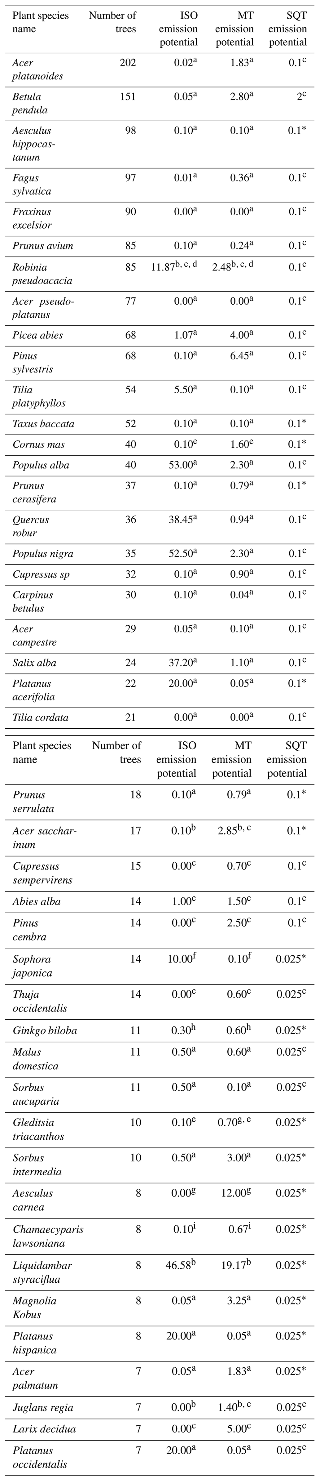
Reference subscripts refer to (a) Stewart et al. (2003), (b) Kesselmeier and Staudt (1999), (c) Karl et al. (2009), (d) Noe et al. (2008), (e) Nowak et al. (2002), (f) Wang et al. (2007), (g) Baghi et al. (2012), (h) Li et al. (2009), and (i) Owen et al. (2003). The asterisk (^*) indicates a standard value of 0.1, as no literature value is available.

For emission potentials, literature values of plant-species-specific emission potentials of isoprene and monoterpene (µg compound g⁻¹ dry-weight h⁻¹) standardized to 303.15 K and PAR of 1000 µmol m⁻² s⁻¹ were assigned to the 44 most abundant species in the study area. This includes all tree species with an occurrence larger than six individuals within the 60 % footprint density and accounts for ∼90 % of the total counted trees. Emission potential assignment was based, if available, on the detailed work by Stewart et al. (2003). Other emission potentials were taken from other literature, and if more than one literature value was available, an average was taken. All species, emission potentials, and references thereof are shown in Table 1. Sesquiterpene (SQT) emission potentials were taken from Karl et al. (2009) and if not reported therein the average value of 0.1 µg compound g⁻¹ dry-weight h⁻¹ was assigned.

2.5 Relative ISO, MT, and SQT emission ratio maps

To generate emission ratio maps, the study area was divided into a 100 m by 100 m grid, and tree species were counted in each grid tile and multiplied by their emission potential listed in Table 1. The resulting map (µg compound g⁻¹ dry-weight h⁻¹) neglects the actual, but unknown, amount of dry leaf weight of each individual tree.

Due to the unknown amount of emitting leaf material, it is difficult to compare bottom-up estimates from this method with direct eddy covariance flux measurements. A more robust comparison is possible when relative emission maps are investigated such as ISO $/$ MT, ISO $/$ SQT, and SQT $/$ MT. For this we first added up all individual tree emission factors in each tile (e.g., ${\mathrm{ISO}}_{\mathrm{tile}}=\sum {\mathrm{ISO}}_{\mathrm{tree}}$) and then divided these by the tile emission factors, e.g. ISO_tile $/$ MT_tile. For simplicity this is called ISO $/$ MT in the following. This is a bottom-up ISO $/$ MT ratio expected at the measurement site. The authors acknowledge that leaf age, phenology, and LAI or individual trees affect this ratio, but these are unknown for the tree inventory and are therefore a source of uncertainty of this estimate. Doubling and halving the emission potential of the highest 20 emitters resulted in average study area emission ratio changes on the order of 5 %–15 %, giving an estimate of the robustness of this analysis.

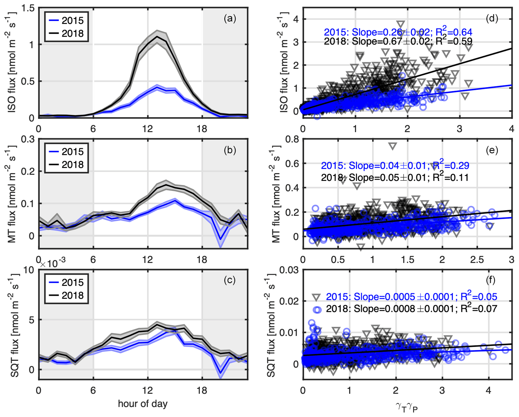
Figure 2 Diurnal cycles of average isoprene (a), monoterpene (b), and sesquiterpene (c) fluxes for the summers of 2015 (blue) and 2018 (black); shaded areas indicate the standard error. Nighttime fluxes are shown here for completeness of the diurnal cycle, but grey shaded areas indicate that these data were not used for further analysis. (d–f) Daytime (06:00–18:00) isoprene, monoterpene, and sesquiterpene fluxes are plotted vs. theoretical temperature and light dependencies (Guenther et al., 2006, 2012) including T24, T240, P24, and P240. The 2015 data are depicted in blue and 2018 data in black. The lines indicate a linear fit, with fit parameters displayed within the plot. The slope of the fit parameter represents the standardized (303.15 K and 1000 PAR) emission factors.

3 Results and discussion

3.1 Flux footprint, light, and temperature conditions

The flux footprint density at the IAO is shown in Fig. 1a and b for 2015 and 2018, respectively. Flux footprint density lines from 30 %–90 % are plotted on a map of 2000 m × 2000 m surrounding the flux tower location. A total of 60 % of the flux footprint density lay, in both years, entirely within the study area (1000 m × 1000 m). The relative contribution of the land cover types within the study are was similar in both years with 40 %–41 % buildings, 23 % paved areas, 25 %–28 % roads, 5 % trees, 5 % short vegetation, and <1 % water. Within the 60 % flux footprint density area in 2015 and 2018 lay 148 and 89 individual trees of the tree inventory distributed over 33 and 24 tree species, respectively. Combining the tree inventory with literature values on basal emission factors (Table 1) and the footprint density calculated for each tree location revealed that 60 % and 70 % of the bottom-up isoprene emissions arriving at the flux tower were from 12 trees in 2015 and 2018, respectively. These were trees closest to the footprint density maximum and trees with high isoprene basal emission factors. The tree species were Populus nigra, Platanus acerifolia, Sophora japonica, and Quercus robur. As the 60 % footprint density area was smaller in 2018 compared to 2015, the relative importance of the emission of these trees was higher in 2018 than in 2015. Bottom-up monoterpene emissions were distributed more evenly among different tree species: 19 trees in the study area accounted for ∼50 % of the bottom-up MT emissions arriving at the flux tower. The most important species were Aesculus carnea, Pinus sylvestris, Larix decidua, and Acer platanoides. Sesquiterpene bottom-up emissions were even more equally distributed over the tree species: 38 trees accounted for 50 % and 60 % of bottom-up SQT emissions arriving at the flux tower in 2015 and 2018, respectively. Betula pendula and Sophora japonica contributed 20 % and 12 % to the emissions arriving at the tower in 2015 and 22 % and 19 % in 2018. Diurnal cycles of PAR and air temperature, two of the strongest biogenic emission drivers, are shown in Fig. 1c and d, respectively. While PAR was very similar during the two summers, mean air temperatures in 2018 were 2 K higher during daytime and 1.5 K higher during nighttime compared to 2015. The higher temperatures in 2018 coincided with an intense heat wave. Monthly average temperatures in August 2018 were 3 K above the climatological mean values (1981–2010).

3.2 Two summers of urban isoprenoid fluxes

Karl et al. (2018) showed that isoprene and monoterpene at this measurement site are linked to biogenic processes. Figure 2a–c show the average diurnal cycles of isoprene, monoterpene, and sesquiterpene fluxes. Mean daytime maxima of isoprene fluxes were 0.4 and 1.2 nmol m⁻² s⁻¹ in 2015 and 2018, respectively. The large interannual difference and its potential reasons are discussed further Sect. 3.3. Anthropogenic contributions to isoprene emissions from traffic were, on the one hand, estimated using the COPERT emission model (https://www.emisia.com/utilities/copert/, last access: 1 August 2021) and 1,3-butadiene as a proxy. We use the ratio of 1,3-butadiene to isoprene from road tunnel studies (Reimann et al., 2000) and multiply this by the modeled 1,3-butadiene to benzene ratio. There is no significant modeled difference between warm and cold seasons because unsaturated hydrocarbons and benzene primarily originate from combustion-related emissions. Relative to benzene we calculate that anthropogenic isoprene emissions contribute on the order of 5 % during daytime (Fig. S5 for the summer season). At night the contribution can be larger (e.g., up to 20 %) as biogenic emissions decrease more rapidly than benzene fluxes. On the other hand, we used the measured wintertime isoprene to benzene flux ratio, which revealed a conservative limit of 20 % due to anthropogenic origin. Overall isoprene emissions are dominated by biogenic emissions at this site. This is in good accordance with previous studies conducted in urban environments (Kota et al., 2014; Park et al., 2010; Rantala et al. 2016).

Maximum average daytime monoterpene fluxes were 0.13 and 0.18 nmol m⁻² s⁻¹ for 2015 and 2018, respectively, and average daytime sesquiterpene fluxes were $\mathrm{5}\times {\mathrm{10}}^{-\mathrm{3}}$ nmol m⁻² s⁻¹ in both years.

The theoretical temperature and light parameters are plotted vs. the observed fluxes in Fig. 2d–f based on the MEGAN big leaf approach (Guenther et al., 2006, 2012.). The slope of the fit parameters represents the standardized (303.15 K and 1000 PAR) emission factors. The slopes in Fig. 2d–f can be interpreted as standardized fluxes, removing the variability due to current and past temperature and light conditions, and allow for interannual comparison as well as comparison to other studies. Standardized isoprene fluxes were 0.26±0.02 nmol m⁻² s⁻¹ and 0.67±0.02 nmol m⁻² s⁻¹ in 2015 and 2018, respectively. The interannual difference is further discussed in Sect. 3.3. Isoprene fluxes from both years were lower than what Rantala et al. (2016) found for an urban flux site in Helsinki, where the standardized emission potential was 125 ng m⁻² s⁻¹ (equal to 1.8 nmol m⁻² s⁻¹). The Helsinki flux site had a larger vegetation cover of 38 %–59 % compared to our study area, where the vegetation cover was estimated to be 10 % within the flux footprint. Park et al. (2010) reported a standard emission rate of isoprene of 0.53 mg m⁻² h⁻¹ (equal to 2.2 nmol m⁻² s⁻¹) over Houston, Texas, which is higher than both our 2018 and 2015 measurements. This is potentially due to a higher vegetation cover in Houston as well as strong isoprene-emitting oaks within the footprint of the measurement site. Valach et al. (2015) reported a daytime average flux in August of 0.3 mg m⁻² h⁻¹ (equal to 1.2 nmol m⁻² s⁻¹) at an urban site in London and Acton et al. (2020) a summer daytime average isoprene flux of 4.6 nmol m⁻² s⁻¹ at an urban site in Beijing; however, neither can be directly compared to our measurements as their values were not standardized to temperature and PAR.

Average daytime standardized monoterpene fluxes were, at 0.04 and 0.05 nmol m⁻² s⁻¹ in 2015 and 2018, respectively, relatively similar between the two summers. Average daytime standardized sesquiterpene fluxes were over a magnitude smaller than standardized monoterpene fluxes and were comparable between the two summers with midday values on the order of $\mathrm{3.0}\times {\mathrm{10}}^{-\mathrm{3}}$ and $\mathrm{3.5}\times {\mathrm{10}}^{-\mathrm{3}}$ nmol m⁻² s⁻¹ in 2015 and 2018, respectively. Both monoterpene and sesquiterpene flux measurements could be underestimated due to loss with reaction to ozone. The values given here could be underestimated by 10 % for monoterpenes and 35 %–45 % for sesquiterpenes (see Sect. 2.2).

Monoterpene and sesquiterpene fluxes measured at lower temperatures (280–295 K) were higher than the predicted values based on biogenic emission parameterizations (data not shown). This could be an indication that at lower temperatures other non-biogenic sources contributed to monoterpene and sesquiterpene fluxes at this site. At temperatures higher than 295 K, MT and SQT fluxes followed known temperature dependencies. To test this hypothesis we considered footprint variations and relative distributions between grasses and trees, which were minor. Variations in flux footprint and a relative distribution with higher grassland MT emissions can be excluded as an explanation for MT and SQT excursions. Instead we find that the residual of non-explained MT and SQT fluxes correlates well with aromatic fluxes. We find a significant positive correlation (R²∼0.75; RMSE: 0.006204) of the residual MT flux with the benzene flux (Fig. S5). It suggests that emission of volatile chemical products (VCPs) (e.g., Gkatzelis et al., 2021) is the most likely explanation for MT and SQT flux enhancements that are not being reproduced by biogenic emission parameterizations.

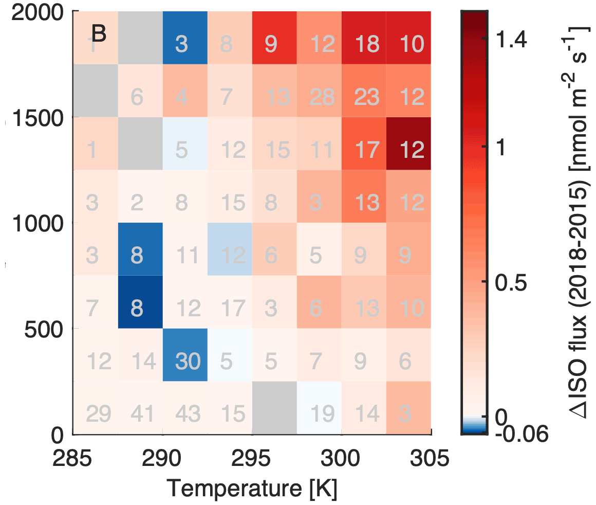
Figure 3 Isoprene flux differences between 2018 and 2015 binned by temperature and PAR; positive differences are shown in red, negative in blue, and bins with no available data are colored grey. Grey numbers in the temperature and PAR fields indicate the number of observations for each temperature and PAR value pair.

3.3 Isoprene flux anomaly

The isoprene flux difference measured between the two summers of 2015 and 2018 is shown in Fig. 2a. Daytime maximum isoprene fluxes in 2018 were up to 2.7 times higher than in 2015. Isoprene fluxes are temperature-dependent (Guenther et al., 1993) and light-dependent (Monson and Fall, 1989), and past 24 and 240 h temperature and light conditions play a role (e.g., Guenther et al., 2006). These theoretical temperature and light parameters are plotted vs. the observed isoprene flux in Fig. 2d based on the MEGAN big leaf approach (Guenther et al., 2006). Even after including both actual and past temperature and light parameters the difference in isoprene fluxes between the two summers could not be resolved, and standardized emission factors were still a factor 2.3 higher in 2018 than in 2015. Figure 3b shows that the difference increased with higher temperature and higher PAR values.

In contrast to monoterpene and sesquiterpene fluxes, which exhibited comparable emission potentials between the two years and are mainly driven by evaporative emissions from storage reservoirs (e.g., Kesselmeier and Staudt, 1999), it remains a puzzle why the isoprene emission potential was substantially higher in 2018 compared to 2015. As neither actual temperature and light dependencies nor 24 and 240 h past temperature and light could fully explain the observed differences in isoprene fluxes, we investigated the following potential reasons: (a) variation in the flux footprint, (b) tree trimming, (c) water availability and/or drought, and (d) emission parameterization.

• a

  Figure 1 (left and middle panel) shows differences in the flux footprint densities between 2015 and 2018. Possible reasons for this are a change in flux tower position between the two years by ∼50 m and different meteorological conditions. In 2015, for westerly winds the flow regime may have been affected by the support structure and the building, and consequently the analysis of isoprenoid fluxes was limited to the northeastern wind sector of [0^∘, 120^∘]. Median daytime wind speed and direction in 2018 (affected by a heat wave) are similar to those in 2015 (Table S1). Median sonic temperature, sensible heat flux, and friction velocity (see Table S1) were higher in 2018, resulting in stronger turbulent vertical transport with mostly friction velocity being responsible for the differences of the flux footprint density function between 2015 and 2018 (Fig. 1). Multiplying the footprint density at each tree location by the basal emission factor of each tree species revealed a potential difference of 24 % higher isoprene emissions in 2018 than in 2015. Even though the actual leaf area of each individual tree is not known and therefore neglected, this 24 % of potential emission difference due to footprint density changes cannot explain the factor of 2.3 in observed fluxes between the two years. Also, growth of juvenile trees between the study years is unlikely to play a significant role, as just 8 % of the strong isoprene emitters were younger than 5 years in 2015. This analysis assumes that the trees from the tree inventory were responsible for the majority of measured isoprene fluxes and that they were more important than emissions from short vegetation (e.g., lawn). Further supporting evidence that the flux footprint change cannot fully explain the observed differences derives from the fact that both monoterpenes and sesquiterpenes did not show significant interannual variations in their normalized emission potentials.

• b

  A second possible explanation for the isoprene flux difference could be differences in LAI in the two seasons, for example due to pruning, early leaf senescence, or insect and/or pathogen damage. Personal communications from city gardeners revealed that of the trees most important for isoprene emissions in the study area (Populus nigra, Populus alba, Quercus robur) only poplar trees were cut differently in 2015 than in 2018. In 2015 only dead wood was removed from the poplars, whereas trees were cut more substantially in 2018. This would, however, lead to an expected smaller flux in 2018 than in 2015 due to reductions in leaf area. No observations on early leaf senescence or leaf damage by insects and/or pathogens were reported by the city gardeners during the two study years.

• c

  A third possible explanation is that the growing season of 2018 was exceptionally dry with lower-than-average precipitation and large-sale, satellite-derived root zone soil moisture (Fig. 4a and b). Concurrent water flux observations, however, shown in Fig. 4c, indicate that on average the 2018 daytime summer water flux was 0.2 mmol m⁻² s⁻¹ higher than in 2015. Also, the total surface water vapor conductance was 50 mmol m⁻² s⁻¹ higher in 2018 than in 2015. Higher water fluxes observed in 2018 agree with anecdotal reports of city trees being artificially watered throughout the summer. Water fluxes in urban areas (maximum Bowen ratios observed in Innsbruck are 6; Karl et al., 2020) are generally very low (e.g., 5–6 times lower) when compared to measurements over purely vegetated surfaces and therefore notoriously difficult to interpret. As such we cannot exclude the possibility of processes other than evapotranspiration from city trees contributing to higher water fluxes observed in 2018. An obvious explanation is that a significant water runoff during extensive watering operations resulted in increased evaporation over hot asphalt and other non-vegetated surfaces, leading to higher water fluxes in 2018. Water was also applied to asphalt surfaces more frequently during mornings to minimize the effect of urban aerosol pollution. The cumulative precipitation for July, August, and September 2015 was 340 and 258 mm for 2018. When taking just overlapping campaign duration data (27 July–2 September), the cumulative precipitation was 158 mm in 2015 and 155 mm in 2018. The precipitation data confirm an overall drier meteorological summer in 2018. It is well established that isoprene production in plants can decouple from photosynthesis during periods of drought and can be sustained by alternative metabolic carbon sources (e.g., Bertin and Staudt, 1996; Pegoraro et al., 2004a, b; Fortunati et al., 2008; Genard-Zielinski et al., 2014; Potosnak et al., 2014; Wu et al., 2015). The exact reason for biochemical regulation of isoprene emissions during drought is not fully unraveled but has been suggested to represent a response for coping with heat stress (Loreto et al., 1998). Isoprene fluxes were observed to increase during the very early onset of drought conditions. For example, Seco et al. (2015) reported an increase in the ecosystem-scale isoprene emission potential about 1 month before significant changes in pre-dawn leaf water potential were observed but when CO₂ uptake was already decreasing. Additionally, they observed that the closing of stomata had a bigger effect on CO₂ than water fluxes because gradual increases in vapor pressure deficit during the evening offset reduced leaf conductance. Isoprene is not controlled by stomata and would not be influenced by any changes in stomatal opening. In addition, their canopy-scale observations suggested a shift of the temperature maximum of isoprene emissions towards higher temperatures from pre-drought to drought conditions. Otu-Larbi et al. (2019) reported a 2.5 fold increase in the isoprene emission potential during the same 2018 heat wave in a UK oak forest. They observed a strong temperature dependence of isoprene concentrations during the heat wave and discuss potential causes such as leaf temperature or rewetting-enhanced emissions. While we do not have representative soil moisture data available for this study, we looked at precipitation data. Otu-Larbi et al. (2019) observed large increases in within- and above-canopy isoprene mole fractions in response to rainfall events after a 6-week drought in a temperate broadleaf forest, which they interpreted to result from enhanced isoprene emissions following the rewetting. We consider rewetting events an unlikely explanation for the observed higher isoprene fluxes in 2018 because, even though rainfall was reduced by half compared to 2015, rain-free time intervals were quite short (between 2 and 7 d), and thus no pronounced rewetting occurred after a long dry period. In fact, the isoprene flux time series suggests lower emissions following rain events. We would like to note that both mono- and sesquiterpene emissions are also controlled by stomatal conductance, which could be expected to affect emission rates during drought periods (see, e.g., Niinemets and Reichstein, 2003). We did not observe significant differences of mono- and sesquiterpene fluxes between the seasons.

• d

  We also examined the impact of the emission model framework on isoprene emissions. Due to the lack of directly measured soil moisture data, which would be hard to interpret in an urban context, the drought effect was not included in the emission model parameterization. Precipitation (Fig. 4a) and large-scale satellite-derived soil moisture data (Fig. 4b) suggest 2018 being drier than 2015, corresponding to a significant heat wave in the summer of 2018. Severe drought conditions would reduce isoprene emissions further and therefore could not explain an increased isoprene emission potential in 2018. However, the fact that evaporative water fluxes were comparable between 2015 and 2018 (and if at all were somewhat higher in 2018) suggests that the trees might not have undergone a severe drought episode in the two years. Mild drought has been observed to lead to increases in isoprene emissions (e.g., Otu-Larbi et al., 2019). To investigate relative changes between emission model frameworks we also set up a MEGAN five-layer canopy model (Guenther et al., 2006) for different scenarios. We recognize that the concept of an LAI for the five-layer model is based on the assumption of a homogeneous vegetation distribution. The resulting fraction of sun vs. shade leaves for urban vegetation might therefore not be fully constrained without complex 3D radiative transfer simulations in urban situations with sparsely distributed vegetation. The prescribed setup, however, was chosen to mimic a high sunlight fraction of the biomass with an overall fraction of 64 %. The model setup was in turn only used to see whether differences between 2015 and 2018 could theoretically be explained by a high sunlight fraction or different temperature response curves. We observed that a shift in T_opt towards higher temperatures helped minimize the observed difference between the two years (e.g., 10 % to 40 %) best. So, for example T_opt set to 313 K could explain about half of the flux enhancement. This would leave predicted isoprene emission fluxes underestimated by about 50 % in 2018. The combination of footprint (24 %) and T_opt (50 %) could bring the isoprene emission potential between 2015 and 2018 to within 37 % uncertainty.

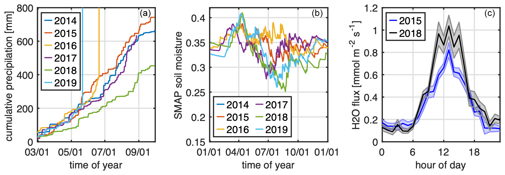
Figure 4 (a) Cumulative precipitation for the growing seasons of 2014–2019. (b) Annual SMAP satellite soil moisture of the root zone from 2014–2019. (c) Diurnal cycle of water fluxes measured in 2015 (blue) and 2018 (black).

3.4 Top-down flux and bottom-up isoprenoid emission ratios

Standardized top-down flux ratios were calculated to allow for a better comparison with bottom-up emission estimates based on literature values of branch-level emissions and a city tree inventory. Top-down (eddy covariance) ISO_S $/$ MT_S flux ratios were on the order of 5 in 2015 and 12 in 2018, again revealing a strong difference between the two years. Top-down MT_S $/$ SQT_S flux ratios were of the order of 30–40 before factoring in losses of sesquiterpenes due to reactions with ozone. Factoring in the upper bound of chemical loss correction, MT_S $/$ SQT_S flux ratios could have been as low as 12–16. Top-down ISO_S $/$ SQT_S flux ratios lay on the order of 190 in 2015 and 380 in 2018, which was mostly caused by the difference in ISO_S flux between the two years. The lower bounds of the ISO_S $/$ SQT_S flux ratios due to fast reaction of sesquiterpene with ozone were 80 and 150 for 2015 and 2018, respectively.

Branch-level standardized emissions are collected from the literature in Table 1 and used to calculate a bottom-up emission map shown in Fig. 5a–c. The 2018 footprint area (Fig. 1a) and therefore footprint density were different to 2015. Multiplying bottom-up emission estimates by footprint density functions, the theoretically expected ISO $/$ MT, MT $/$ SQT, and ISO $/$ SQT ratios in 2015 were 3.6, 5.1, and 18.7, respectively. Multiplying the 2018 footprint density, the values were slightly different at 4.2, 4.6, and 19.2 for ISO $/$ MT, MT $/$ SQT, and ISO $/$ SQT ratios, respectively.

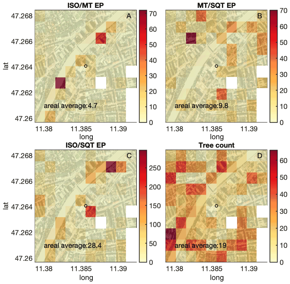
Figure 5 (a–c) Bottom-up estimates of standardized ISO $/$ MT, MT $/$ SQT, and ISO $/$ SQT emission ratios based on literature values (see Table 1). (d) Tree count. Maps were created in MATLAB (https://www.mathworks.com, last access: 1 August 2021) and are based on OpenStreetMap (https://www.openstreetmap.org/copyright, last access: 1 August 2021) under the CC BY 3.0 AT license.

The bottom-up ISO $/$ MT emission ratio was close to the top-down ratio of 2015. This again indicates that 2018 was an exceptional year. In contrast, the bottom-up MT $/$ SQT and ISO $/$ SQT emission ratios were significantly lower than the top-down measured flux ratios of both summers. Even after accounting for the chemical loss of sesquiterpene before it reached the point of measurement at the top of the building, the bottom-up estimates were still higher than the top-down measured flux ratios. Literature values for leaf-level sesquiterpene emissions are rare and were for many species estimated in Table 1. Further extensive studies on sesquiterpene standardized emissions for a large variety of plant species are needed to close the gap between bottom-up emission ratios and top-down flux ratio estimates.

4 Summary

In this study we found a strong correlation of isoprene fluxes with temperature as well as isoprene fluxes following the previously observed leaf-level light dependency. Assuming the same correlation between isoprene and benzene fluxes in early spring before the start of the vegetation period and the summer months results in a maximum of 20 %–30 % influence of anthropogenic sources on isoprene emissions during both the 2015 and 2018 summer measurement periods. A PMF analysis at this site (Karl et al., 2018) has previously revealed two biogenic factors: one light- and temperature-dependent for isoprene and a second mostly temperature-dependent including monoterpenes and sesquiterpenes. Bottom-up emission estimates based on a city tree inventory and emission factors from the literature showed reasonable agreement with standardized ISO $/$ MT flux ratios and an underestimation of standardized MT $/$ SQT and ISO $/$ SQT flux ratios. Interannual comparison of biogenic fluxes revealed up to 3 times higher isoprene fluxes in 2018, when a heat wave persisted, than in 2015. Monoterpene fluxes were an order of magnitude lower than isoprene fluxes, and sesquiterpene fluxes were another order of magnitude lower than monoterpene fluxes; however, both summer fluxes were comparable for these two terpenoid classes after standardization. Our findings show a higher interannual variability of isoprene emissions compared to monoterpenes and sesquiterpenes. Normalizing isoprene fluxes to standard light conditions did not fully remove the interannual difference but decreased the factor from 3 to 2.3. The difference increased with higher temperature and higher PAR values. Analysis of footprint, precipitation, a coarse-scale satellite-based soil moisture product as a proxy for plant water availability, and pruning activity differences of the two summers did not completely resolve the observed differences in isoprene fluxes. Detailed analysis using standard emission modeling concepts suggested a higher-than-expected variation of urban isoprene emission potentials during the heat wave in 2018. While water flux measurements did not indicate a severe drought in 2018, the effect of an intense heat wave in 2018 (2 K higher temperatures on average compared to 2015) likely resulted in enhanced isoprene emissions. Isoprene emissions during drought stress have been grouped into two distinct phases (Niinemets, 2010; Potosnak et al., 2014) and can be enhanced under pre-drought conditions (Seco et al., 2015; Otu-Larbi et al., 2019). Enhanced leaf temperatures (e.g., Potosnak et al., 2014) can explain part of the variance in isoprene emissions, but significant differences remained. In addition to the leaf temperature effect, Tattini et al. (2015) reported an upregulation of isoprene emissions during drought stress as antioxidant defense in Platanus x acerifolia plants. Here a change in T_opt towards a higher temperature optimum could explain another 50 % of the observed isoprene emission flux difference between 2015 and 2018. In conjunction with changes in flux footprints (24 %) these two effects could account for about ∼75 % of the difference. If generalized, our observations suggest distinct differences that urban trees experience, possibly due to significantly altered environmental conditions (e.g., stresses, light, and temperature environment). Vegetation in urban areas is exposed to a variety of different atmospheric conditions, for example the urban heat island effect, high levels of NO_y, heavy metal deposition, or high loadings of aerosols (e.g., black soot). Isoprene emissions have been linked to the plant's nitrogen metabolism (e.g., Rosenstiel et al., 2008); higher leaf nitrate can lead to lower isoprene emissions. Nitrogen dioxide concentrations have been falling in Innsbruck and were 20 % lower in 2018 than in 2015. Effects of air pollutants on leaf surface characteristics and senescence were also reported in the past (Jochner et al., 2015; Honour et al., 2009), but a quantitative understanding of the impacts on isoprene emissions remains unclear. Our observations suggest that more work is needed to improve our understanding of urban biogenic isoprene emissions.