the Creative Commons Attribution 4.0 License.
the Creative Commons Attribution 4.0 License.
 | 03 Jan 2022
Impact of non-ideality on reconstructing spatial and temporal variations in aerosol acidity with multiphase buffer theory
Guangjie Zheng
Siwen Wang
Andrea Pozzer
Aerosol acidity is a key parameter in atmospheric aqueous chemistry and strongly influences the interactions of air pollutants and the ecosystem. The recently proposed multiphase buffer theory provides a framework to reconstruct long-term trends and spatial variations in aerosol pH based on the effective acid dissociation constant of ammonia (). However, non-ideality in aerosol droplets is a major challenge limiting its broad applications. Here, we introduced a non-ideality correction factor (cni) and investigated its governing factors. We found that besides relative humidity (RH) and temperature, cni is mainly determined by the molar fraction of NO in aqueous-phase anions, due to different NH activity coefficients between (NH4)2SO4- and NH4NO3-dominated aerosols. A parameterization method is thus proposed to estimate cni at a given RH, temperature and NO fraction, and it is validated against long-term observations and global simulations. In the ammonia-buffered regime, with cni correction, the buffer theory can reproduce well the predicted by comprehensive thermodynamic models, with a root-mean-square deviation ∼ 0.1 and a correlation coefficient ∼ 1. Note that, while cni is needed to predict levels, it is usually not the dominant contributor to its variations, as ∼ 90 % of the temporal or spatial variations in are due to variations in aerosol water and temperature.
- Article
(7698 KB) - Full-text XML
-
Supplement
(1990 KB) - BibTeX
- EndNote


Aerosol acidity strongly influences the thermodynamics and chemical kinetics of atmospheric aerosols and is therefore one essential parameter in evaluating their environmental, health and climate effects (Pye et al., 2020; Zheng et al., 2020). However, direct measurements of aerosol pH in the real atmosphere are not available so far (Pye et al., 2020; Li et al., 2020). The fast equilibrium with ambient air, tiny volume, and high ionic strength and nucleation potential are the main challenges for measurements, especially online or in situ measurements. Several groups are developing new techniques for this purpose (Wei et al., 2018; Craig et al., 2018; Li et al., 2020; Ault, 2020). For example, Wei et al. (2018) developed an in situ Raman microscopy method for pH measurements in microdroplets (diameter ∼ 20 µm), with an uncertainty of ∼ 0.5 pH units. Craig et al. (2018) and Li et al. (2020) developed colorimetric analyses on pH-indicator papers for aerosol pH measurement, which exhibit uncertainties of around 0.4–0.5 pH units. These currently available techniques, however, still need to be developed further for real atmospheric applications.
Due to the lack of direct measurements, modeling tools have been intensively used to calculate the aerosol pH (Fountoukis and Nenes, 2007; Fountoukis et al., 2009; Clegg et al., 2001; Zuend et al., 2008). The results of thermodynamic models are subject to uncertainties in the input parameters (Fountoukis et al., 2009; Pye et al., 2020; Weber et al., 2016; Guo et al., 2016; Guo et al., 2018; Pye et al., 2018; Tao and Murphy, 2019; Hennigan et al., 2015; Guo et al., 2015; Peng et al., 2019). For example, Hennigan et al. (2015) revealed the importance of including gas-phase species in the input, in addition to the full aerosol composition measurements (Fountoukis et al., 2009). Guo et al. (2015) suggests overall uncertainties of ∼ 0.2–0.5 pH units related to aerosol composition. Pye et al. (2020) reviewed major thermodynamic models and showed that the estimated acidity among different models was on average 0.3 pH units but sometimes as much as 1 pH unit.
The recently proposed multiphase buffer theory shows that globally most of the populated urban areas are within the multiphase ammonia-buffered regime (Zheng et al., 2020). In the buffered regions and/or periods, p can serve as a proxy of aerosol pH, where is the effective acid dissociation constant of NH3 in multiphase systems (Sect. 2). Ideally, p is fully determined by aerosol water content (AWC) and temperature. However, the non-ideality in aerosols may introduce deviations from the ideal conditions. Here we investigated such deviation and derived a non-ideality correction factor for using p as a proxy of aerosol pH. Governing factors of the non-ideality correction factor in aerosol droplets are further explored and discussed, based on which a parameterization method to estimate the non-ideality correction factors is proposed. We also estimated that a constant correction factor of p is often good enough to predict pH over a period at a given site or to explain the global pH variations. We thereby provided a way for pH retrieval when chemical measurements are unavailable for the ammonia-buffered regions and periods.
2.1 Effective acid dissociation constant as a proxy of aerosol pH
2.1.1 Acid dissociation constant of NH3 in bulk solutions, Ka
The definition of acids and bases have been evolving over time. The pioneering Arrhenius theory defined a base as a substance that dissociates in water to form hydroxide (OH−) ions (Pfennig, 2015). Therefore, an Arrhenius base can be expressed as BAOH, which dissociates in water as
with the corresponding base dissociation constant Kb being
In combination with the water dissociation of
the corresponding acid dissociation constant, defined as , is thus (Eqs. 2–1)
The later Brønsted–Lowry theory defined a base as a proton acceptor (Pfennig, 2015) and is expressed as BBL here. In this sense, an Arrhenius base BAOH is not regarded as a Brønsted base but rather as salts. The dissociation reaction for a Brønsted base is expressed as
and the corresponding Ka is thus (Eqs. 2–4)
As NH3(aq) is actually the water adduct of NH3, it is often expressed equivalently as NH3(aq) = NH3•H2O(aq) = NH4OH(aq). In this sense, it can fit in the category of both definitions. In the Arrhenius definition, the base BAOH = NH4OH, namely BA= NH. Therefore, is (Eq. 3)
while with the Brønsted–Lowry definition, the base is BBL=NH3(aq), and is (Eq. 5)
which is the same as Eq. (6). Therefore, a different definition of bases for the ammonia family (BA= NH or BBL = NH3(aq)) will lead to the same expression of , as defined in Zheng et al. (2020). The same applies for other volatile weak bases.
2.1.2 Ideal multiphase acid dissociation constant of NH3
The multiphase effective acid dissociation constant of NH3 under ideal conditions, , depends only on AWC and temperature as (Zheng et al., 2020)
where AWC is in micrograms per cubic meters and is mainly determined by air particulate matter concentrations and RH. The ρw is water density in micrograms per cubic meter, and AWC ρw represents the aerosol water volume mixing ratio in the air in (m3 water)(m3 air). The [NH3(g)] represents equivalent molality (in mol kg−1) of gaseous NH3 in solution (see details in Zheng et al., 2020). The is Henry's law constant of NH3 in mol L−1 atm−1, R is the gas constant of 0.08205 atm L mol−1 K−1, and T is temperature in K.
For typical ambient conditions when AWC varies between 1 to 1000 µg m−3, the [NH3(g)] is usually 105 to 108 times larger than [NH3(aq)], and the above equation can be simplified into
Taking negative lognormal on both sides, we have a pH that is related to p (i.e., −log) as (Zheng et al., 2020)
The multiphase buffer capacity of the NH3–NH pair reached its local maximum when pH = p, namely when [NH3(g)] = [NH(aq)]. At a given AWC and T, is constant.
2.2 Influences of non-ideality on aerosol pH
For ambient aerosols, the ionic strength (I) is high, and the non-ideality must be considered. Under such non-ideal conditions, the multiphase equilibrium of NH3 should be expressed as (Zheng et al., 2020)
where γX is the activity coefficient for species X. Note that Eq. (8a) is the simplified expression of Eq. (9) under ideal conditions when all activity coefficients are unity.
Activity coefficients for gases, like , are usually treated as unity. Again, for typical ambient conditions [NH3(g)] is much larger than [NH3(aq)], and [NH3(aq)] can be omitted. Equation (9) can thus be simplified into
Under non-ideal conditions, pH is usually defined by the proton activity; i.e.,
However, in thermodynamic models that are most commonly applied in current global models (ISORROPIA II, MOSAIC, etc.), the pH is usually defined as free-H+ molality (Pye et al., 2020); i.e.,
The difference in activity- and molality-defined pH (i.e., pHa and pHF) has been discussed in a previous study (Pye et al., 2020), which shows that deviations of pHF from pHa are larger at lower RH and are usually within 1 unit when RH > 60 % (Pye et al., 2020). To be comparable with results in previous studies, the pH we discuss hereinafter follows the free-H+ molality definition. Discussion based on activity-defined pH is detailed in Appendices A and B.
Now we define the multiphase effective acid dissociation constant under non-ideal conditions, , as
which is related to the constant under ideal conditions, , by (Eqs. 9, 10, 12 and 13)
And the free-H+ molality pH is therefore (Eqs. 13a, b)
We now define the non-ideality correction factor cni to represent the difference in pH caused by non-ideality. Based on Eqs. (8b) and (13c), cni is therefore
And combining Eqs. (13b) and (14a), we have
Equation (14b) shows the intrinsic determining factors of cni, i.e., and . Major influencing factors of cni are therefore those influencing the activity coefficients (see Sect. 3.1).
When and are not available, the cni can be alternatively calculated by (Eq. 13a, b)
Equation (14c) is valid as [NH3], [NH] and [H+] concentrations will vary as a result of changing cni. Note that while [NH3] [NH] and pH variations can reflect the cni variations and therefore can be used to derive cni, they are not the determining factors of cni. As shown in Eq. (14b), cni is determined by and , which further depends mainly on RH, temperature and the fraction of NO in anions (see Sect. 3.1).
For some thermodynamics models that predict both the activity coefficients of ions and the gas–particle partitioning of species like the E-AIM model (Sect. 2.3), cni can be derived either from Eq. (14b) (activity-based) or Eq. (14c) (gas–particle partitioning based). However, current atmospheric chemical transport models usually adopted the more computation-efficient thermodynamic models (ISORROPIA II, MOSAIC, etc.), in which only the mean activity coefficient of an electrolyte species ij in water, γij, is derived, where i is a cation, while j is an anion (Pye et al., 2020; Fountoukis and Nenes, 2007; Zaveri et al., 2005). For these models, we cannot directly derive or , and cni is derived through Eq. (14c) (i.e., from the predicted [NH3], [NH], [H+] and AWC).
2.3 Model simulations
Thermodynamic models. Here we used the E-AIM model (model IV; http://www.aim.env.uea.ac.uk/aim/aim.php, last access: 18 November 2021) (Clegg et al., 1992; Wexler and Clegg, 2002; Friese and Ebel, 2010) to predict both the activity coefficients for individual ions and the gas–particle partitioning. The E-AIM model adopted the Pitzer–Simonson–Clegg model (Clegg et al., 1992, 1998) to calculate single-ion activity coefficients, which includes most comprehensive conditions and has been used as a benchmark (Clegg et al., 1992; Hennigan et al., 2015; Pye et al., 2020). Therefore, both the activity-based pH (pHa, Eq. 11) and the free-H+ molality pH (pHF, Eq. 12) can be derived (Appendix B). In addition, we also adopted the ISORROPIA v2.3 model (Fountoukis and Nenes, 2007) for comparison, which is computational effective and has been commonly adopted in global and regional models. To reduce the computational cost, the ISORROPIA model calculated only the binary activity coefficients γij using the Kusik–Meissner relationship and Bromley's formula (Fountoukis and Nenes, 2007). Therefore, only the free-H+ molality pH (pHF, Eq. 12) can be derived in ISORROPIA (Appendix D). For example, for a HCl droplet, both γH+(aq) and γCl-(aq) are calculated in E-AIM, while only the mean binary activity coefficient of is estimated in ISORROPIA.
Global models. Spatial variation in cni was studied based on the two global models. The global GEOS-Chem model simulations (v11-01) were conducted at a resolution of 2∘ latitude × 2.5∘ longitude with 47 vertical layers for 2016. Detailed model settings are provided elsewhere (Zheng et al., 2020). The global EMAC (ECHAM5/MESSy2 for Atmospheric Chemistry) model was run at a resolution of T63 (i.e., ∼ 1.8∘ × 1.8∘ at the Equator) with 31 vertical levels for 2016. Detailed EMAC model settings are provided in Appendix C.
3.1 Influencing factors of the non-ideality coefficient
All activity coefficients first depends on RH and temperature. In addition, for ammonium-buffered ambient aerosols, major anions paired with NH or H+ are NO and SO. The ratio of mean activity coefficients is therefore expected to differ when they are mainly combined with SO (i.e., ) or NO (i.e., ).
Figure 1 shows the dependence of cni under different systems (Appendix A), as predicted by the gas–particle portioning (Eq. 14c) with E-AIM (Fig. 1a, c, e) and ISORROPIA II (Fig. 1b, d, f). Based on both models, cni differs much between the NH3–H2SO4 system (Fig. 1a, b) and the NH3–HNO3–H2SO4 system (Fig. 1c, d), even at the same RH and temperature. The difference is still large when compared at the same ionic strength and temperature (Fig. A1), illustrating that the difference is mainly due to the ion-pair specific binary activity coefficients, (Zaveri et al., 2005; Fountoukis and Nenes, 2007; Clegg et al., 1992) (Appendix B; Fig. B1).

Figure 1The non-ideality correction factor, cni, estimated by E-AIM (a, c, e) and ISORROPIA (b, d, f) for different aerosol systems. (a, b) NH3–H2SO4–H2O system with aerosols dominated by (NH4)2SO4 at varying RH and temperature conditions; (c, d) NH3–HNO3–H2O system with aerosols dominated by NH4NO3 at varying RH and temperature conditions, and (e, f) Na+–NH3–HNO3–H2SO4–H2O system with varying chemical profiles at 288.15 K and RH of 73 %. The chemical profiles in (e) and (f) are characterized by the fraction of NO in anions(aq) and NVCs anions(aq), where the non-volatile cations (NVCs) are assumed to be Na+ only here. The assumed RH and T conditions in (e) and (f) are marked as blacked stars in (a)–(d), while the chemical profiles of (a)–(d) are marked by the corresponding letter in (e) and (f), respectively.
Due to the large difference in cni between NH4NO3 and (NH4)2SO4-dominated aerosols, the cni at a given RH and temperature conditions is therefore sensitive to the anion profiles, as characterized by the fraction of NO in anions(aq), , of
The is proportional to NOSO molar ratios when Cl− is negligible. In comparison, the cation profiles, or the relative abundances of non-volatile cations (NVCs; total cations from Na+, Ca2+, K+ and Mg2+), play a minor role as their influence is more indirect (Fig. 1e, f).
3.2 Comparison of cni estimated by E-AIM and ISORROPIA
As discussed in Sect. 2.2, for E-AIM cni can be estimated either by activity coefficients (Eq. 14b) or gas–particle portioning (Eq. 14c), and the results agreed perfectly (black lines in Fig. 2). Therefore, the cni estimation with E-AIM is calculated by the gas–particle portioning (Eq. 14c) hereinafter, the same as for ISORROPIA.
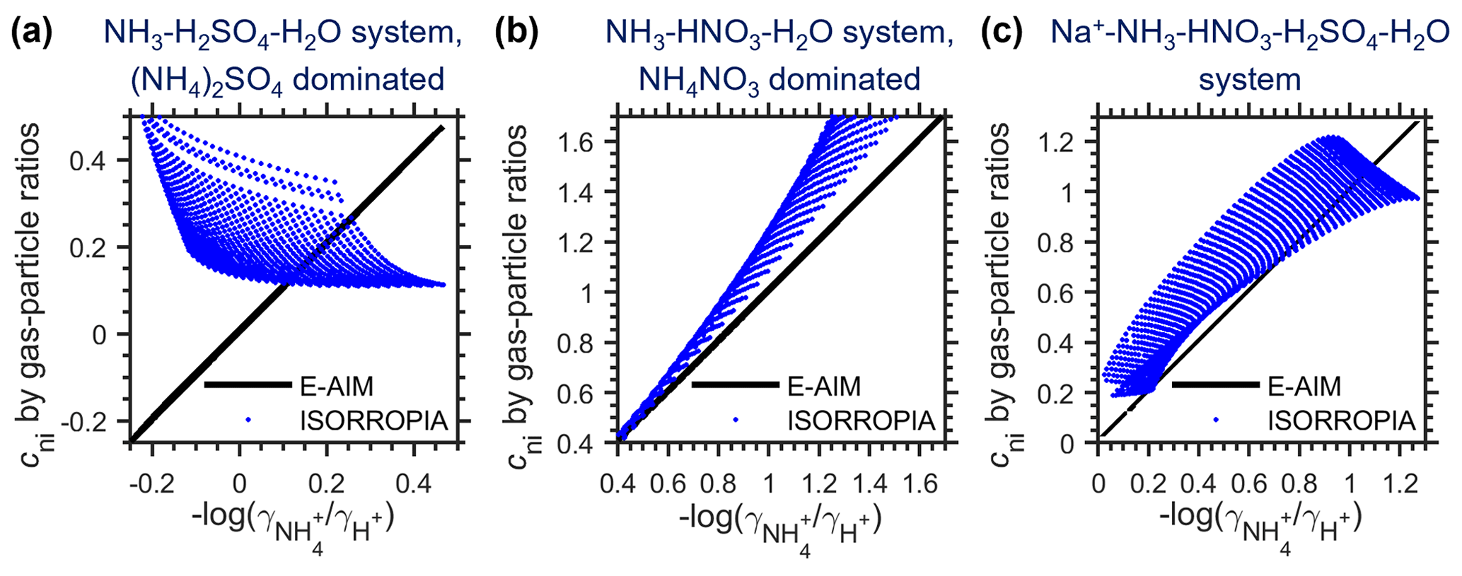
Figure 2Comparison of different cni estimation methods for three representative aerosol systems. The cni are compared under the same conditions (i.e., same RH, temperature and chemical profiles). The x values are cni estimated by activity coefficients (Eq. 14b) with the E-AIM model, and the y values include cni estimated by gas particle ratios (Eq. 14c) with the E-AIM (black lines) and ISORROPIA (blue dots) models. The systems are the same as in Fig. 1.
Although showing the same influencing factors, cni estimated by E-AIM and ISORROPIA is not identical (Fig. 1). Especially for the NH3–H2SO4–H2O system (i.e., (NH4)2SO4-dominated aerosols), E-AIM (Fig. 1a) and ISORROPIA (Fig. 1b) even predicted reversed trends in cni dependence on RH and temperature. This is more clearly shown in Fig. 2 (blue dots), where cni by E-AIM and ISORROPIA in the same conditions (i.e., same RH, temperature and chemical profiles) is compared. As shown in Fig. 2a, while cni predicted by E-AIM ranged −0.3 to 0.5 for (NH4)2SO4-dominated aerosols, that predicted by ISORROPIA was always larger than 0.1. This is mainly caused by the difference in calculated activity coefficients between ISORROPIA and E-AIM (Eq. 14b; see details in Appendix D, Figs. D1 and D2).
Despite the large difference in predicted cni for the NH3–H2SO4–H2O system, the E-AIM and ISORROPIA models generate similar predictions of AWC and therefore a similar ideal constant of (Fig. D1a). Combined with different cni, this would lead to a different prediction of [H+(aq)][NH3(g)][NH(aq)] by the two models (Eq. 14c). However, with the constraint of charge balance and mass conservations of ammonia (Appendix D), the disagreement in the predicted molar ratios of NH3(g)NH(aq) between these two models is relatively small (4 %–6 %; Fig. D1b), and most of the cni variations are allocated to the [H+], or pH, predictions (Fig. D1c).
Unlike the NH3–H2SO4–H2O system, cni estimated by ISORROPIA generally agrees well with E-AIM when HNO3 is present in the system (Fig. 2b, c), although it tends to be somewhat higher than E-AIM. This indicates that constraints from NH3–HNO3 equilibriums are quite important in estimating cni with ISORROPIA (see details in Appendix D). Under ambient conditions, there is barely places with negligible HNO3, thus the ISORROPIA-predicted cni generally agreed with E-AIM (Sect. 3.4).
With the known governing factors, here we propose a parameterization method to estimate cni at a given RH, temperature and , with lookup tables generated by comprehensive thermodynamic models, E-AIM and ISORROPIA (“AIM_molality” database and “ISORROPIA_molality” database as in Data S1). In addition, the parameterized cni for activity-based pH (Eq. 11; Appendix B; Fig. B1) is also available (“AIM_activity” database in Data S1). A Matlab code to get cni is also provided (Data S1). Example slices of this cni parameterization based on AIM_molality estimations are shown in Fig. 3. Note that this parameterization method is aimed at the NH3–HNO3–H2SO4–H2O system, assuming no NVCs. We will show that this assumption is acceptable under most cases in the following sections.
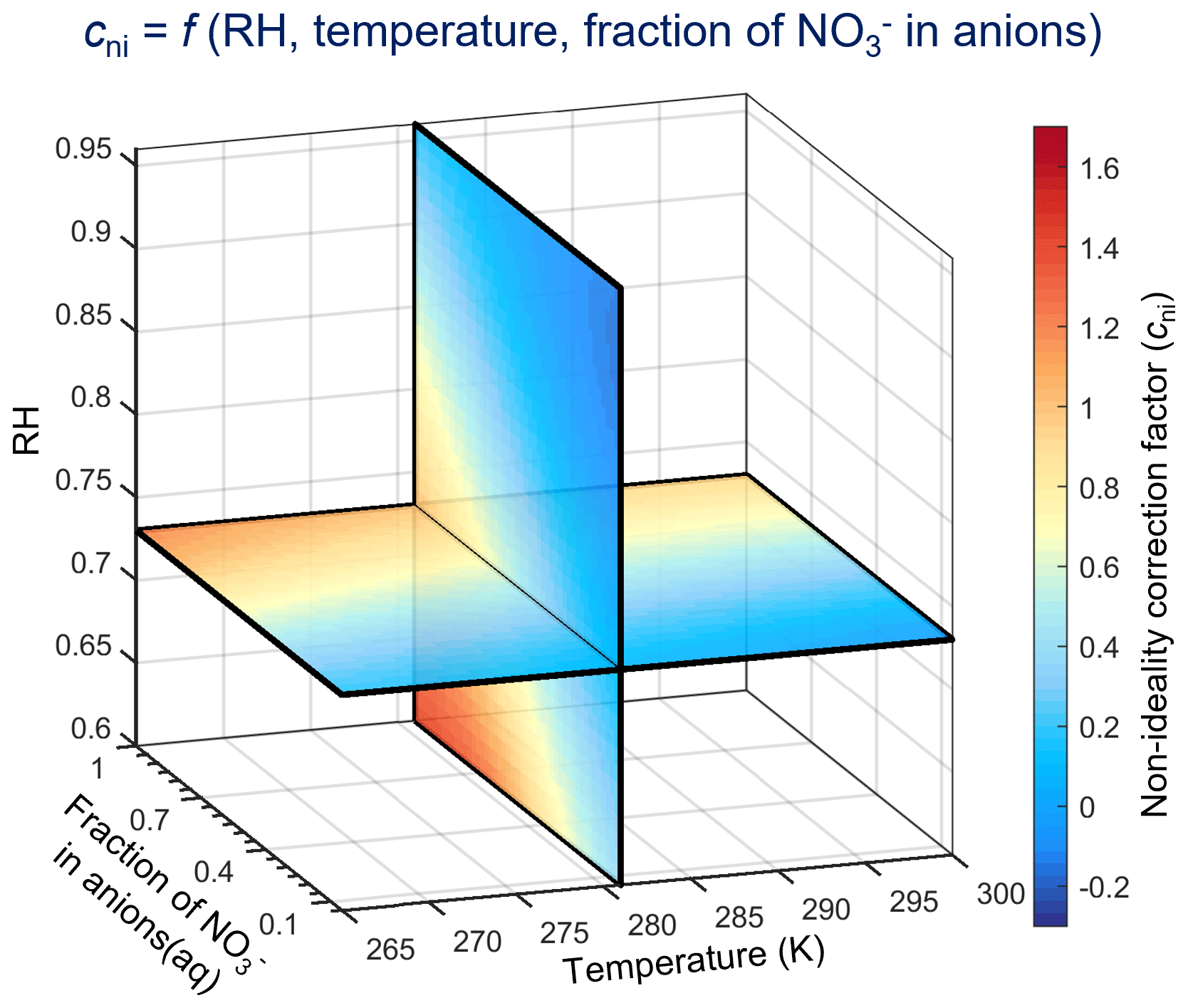
Figure 3Example slices of the cni parameterization based on “AIM_molality” estimations as given in Data S1 in the Supplement.
3.3 Validation and applications with long-term observations
To validate the cni parameterization method under actual ambient conditions, we here show an example application based on the long-term measurements in Toronto (Tao and Murphy, 2019) (Fig. 4). From 2007 to 2016, Toronto resides in the ammonia-buffered regime for ∼ 80 % of the time, and the model-predicted pH based on the measured chemical compositions follows nicely with the variation in actual p estimated by thermodynamic models (Eq. 14), for both E-AIM (Fig. 4a) and ISORROPIA (Fig. 4c). Parameterized cni agreed quite well with the actual ones for both models (Fig. 4b, d, black circles), with R2 being 0.99 in both cases and the both corresponding root-mean-square deviations (RMSDs) being ∼ 0.1.
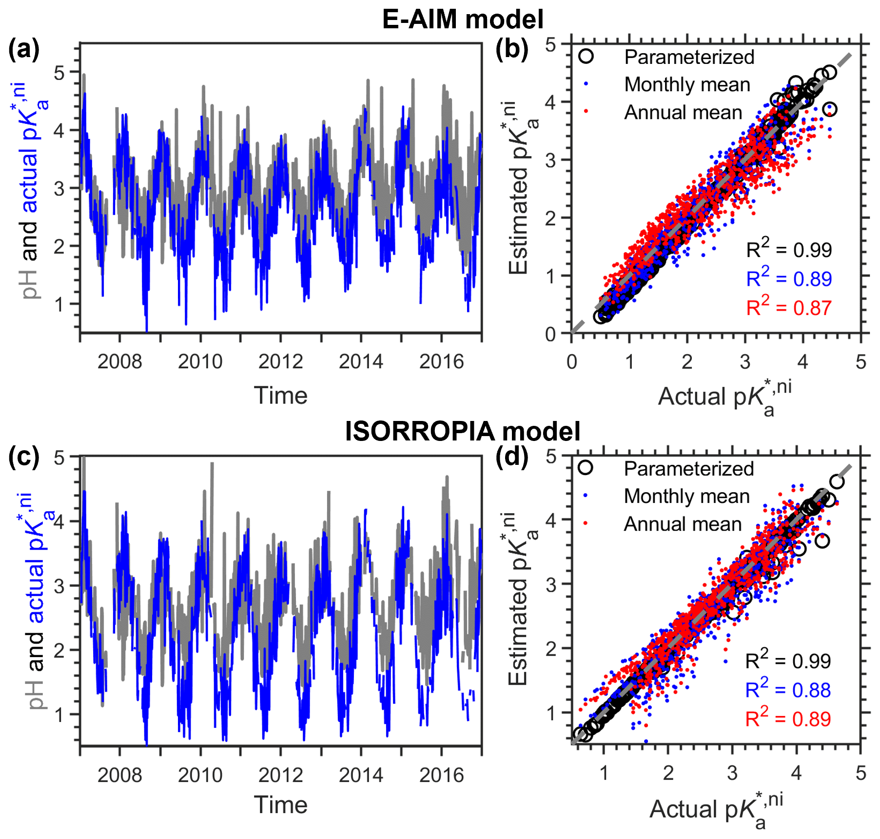
Figure 4Comparison of pH and actual and estimated p based on the 10-year observations in Toronto. Data were taken from Canada's National Air Pollution Surveillance (NAPS) Program, as detailed in Tao and Murphy (2019). Predications are based on (a–b) the E-AIM model and (c–d) the ISORROPIA model. The “parameterized” series in (b, d) are predicted by the parameterization method proposed with the input of the observed RH, temperature and model-predicted fraction of nitrates in anions. The annual mean and monthly mean are based on mean cni of an arbitrary example year of 2012.
Figure 4 also suggests that most of the variation in actual p comes from the variation in ideal constants (p), not the non-ideality. For example, now we assume the full aerosol and gas measurements were conducted only in a calibration year of 2012, based on which the annual mean and monthly mean cni can be derived (Fig. E1). Annual mean cni is 0.4 for E-AIM and 0.8 for ISORROPIA estimations. When we use the annual mean cni as a constant correction (i.e., estimated p p annual mean), fluctuation in the estimated p would actually all come from p. However, this estimated p can already explain ∼ 90 % of the variations in actual p (red dots in Fig. 4b, d), illustrating the dominance of p (i.e., AWC and temperature fluctuations) over non-ideality. In comparison, applying the month-dependent cni values (blue dots in Fig. 4b, d) makes little difference with the annual constant estimations (R2 differed only by 1 %).
Figures 4 and E1 illustrate that a constant cni is often good enough at a given site. Full aerosol species measurements for a whole year, or under periods representative of annual-average conditions (like spring or fall seasons for Toronto; Fig. E1), are recommended in determining the localized cni, which, together with AWC and temperature measurements, could already provide a good approximation of the aerosol pH. This is especially useful in retrieving the acidity variations when full chemical measurements are not available in the long run.
3.4 Validation and application against global model simulations
We further investigated the influence of non-ideality in explaining the spatial variations in aerosol acidity based on global model simulations. On the global scale, the fraction of NO in aqueous-phase anions depends on two factors: the total nitrate (gas + particle phase) to sulfate ratios and the partitioning of total nitrates. When total nitrate ≪ sulfates, the aerosols would be dominated by (NH4)2SO4 even if all the nitrates are partitioned into the particle phase. In this case, a non-ideality correction factor can be estimated from Fig. 1a and b at known RH and temperature. However, both GEOS-Chem and the EMAC results show that this criterion is barely met for the ammonia-buffered regions. Besides, for all the reported observation results we know of, only the summertime southeastern US (Weber et al., 2016) has a total nitrate that is < 5 % of the sulfate (charge ratios). Therefore, under most conditions, cni largely depends on the partitioning of total nitrates, and an estimation of is needed to derive the correction factor.
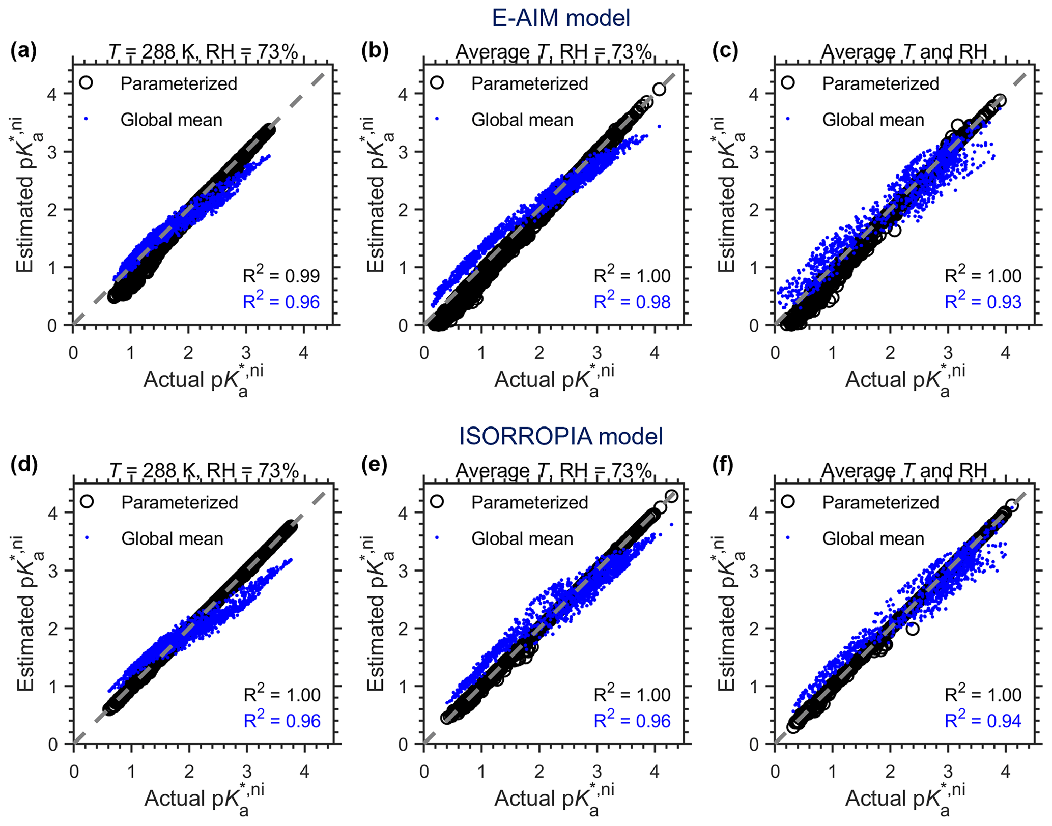
Figure 5Comparison of actual and estimated p based on the GEOS-Chem global simulations in 2016. Predications are based on (a–b) the E-AIM model and (c–d) the ISORROPIA model. The “parameterized” series are based on the parameterization method proposed in this study, while the global means are based on mean cni calculated from thermodynamic models under each scenario.
Figure 5 shows the estimated p against actual p based on GEOS-Chem simulations, and that based on EMAC simulations is shown in Fig. C1. Three scenarios are assumed to examine the sensitivity of p prediction with cni values: (a) constant temperature (T) of 288 K and RH of 73 %, (b) constant RH of 73 % but with annual-average temperatures for each site, and (c) annual-average T and RH for each site. For all scenarios, annual mean chemical compositions for the ammonia-buffered surface regions (Zheng et al., 2020) are used, and cni is estimated by both E-AIM and ISORROPIA II models. Similar to Fig. 4, in the “parameterized” series cni is estimated by the parameterization method proposed in this study with RH, T and at certain model grids, while in the “global mean” series, cni is assumed to be constant as the average of actual cni estimated by the thermodynamic models under each scenario, which is ∼ 0.6 for the E-AIM model and ∼ 0.8 for the ISORROPIA model.
Based on GEOS-Chem simulations, the parameterized cni (black dots in Fig. 5) work nicely in reproducing actual p, with R2 near 1 under all scenarios and the RMSD of < 0.03 for the ISORROPIA model and ∼ 0.1 for the AIM model. Again, we found that variations in cni are much smaller than the variation in p caused by particulate matter concentrations and temperatures. With a constant global-mean cni correction (i.e., assuming a global average ) (blue dots in Fig. 5), the estimated p can already explain over 93 % of the variations in actual p, with/without considering the influence of meteorology on non-ideality alike. Correspondingly, it can already explain ∼ 70 % of the aerosol pH variations (Zheng et al., 2020), where the pH is further subject to variations in NH3(g) and NVCs (Eq. 8; Zheng et al., 2020).
The EMAC simulations show similar patterns with GEOS-Chem results. Estimated p with the parameterized cni corrections agreed well with actual p, with R2 over 0.94 for the E-AIM model and over 0.91 for the ISORROPIA model (Fig. C1). This is somewhat lower than the Toronto site (Fig. 4) or the GEOS-Chem result (Fig. 5), which is due to the larger variations in the simulated chemical profiles (e.g., importance of NVCs and Cl−). The constant cni assumption (blue dots in Fig. C1) works similarly with the parameterized ones when the influence of meteorology is excluded (Fig. C1a, d) or when spatial variations in temperatures are considered (Fig. C1b, e). When spatial variations in both temperature and RH (Fig. C1c, f) are considered, the constant cni assumption works worse than the parameterized ones but is still acceptable (R2 being 0.75 for E-AIM and 0.69 for ISORROPIA).
Note that under all conditions, the global mean method tends to overestimate cni when the actual p of NH3 is smaller than 2 (Figs. 5, C1). That is caused by . The low p indicates low AWC levels (Zheng et al., 2020) and relatively low pH levels (Eq. 13). Under such conditions, HNO3 tends to stay in the gas phase (Nenes et al., 2020), corresponding to a low of ∼ 0. In comparison, the global-mean cni corresponds to the global-mean simulated of ∼ 0.4. As cni increases with increasing (Fig. 1e, f), the global-mean cni would tend to overestimate actual low p conditions (i.e., < ∼ 2).
Overall, we found that the non-ideality correction is needed for using p of NH3 as a proxy of aerosol pH in ammonia-buffered regimes. This correction factor, cni, generally ranges from 0.3–1.1 and mainly depends on RH, temperature and the fraction of nitration in aqueous-phase anions. E-AIM generally predicted a lower cni than the ISORROPIA model. We proposed a parameterization method to estimate the cni, which works quite well, as validated against both long-term observations and global simulations. Although the correction is needed in estimating the ammonia p levels, the variations in p is often much less sensitive to the non-ideality than to aerosol water content and temperature. Therefore, a constant correction factor of p is often good enough to predict pH over a period at a given site, or to explain the global pH variations. We thereby provided a way for pH retrieval when chemical measurements are unavailable for the ammonia-buffered regions.
In Figs. 1, 2, A1, B1, D1 and D2, we assumed three systems, with the settings detailed below.
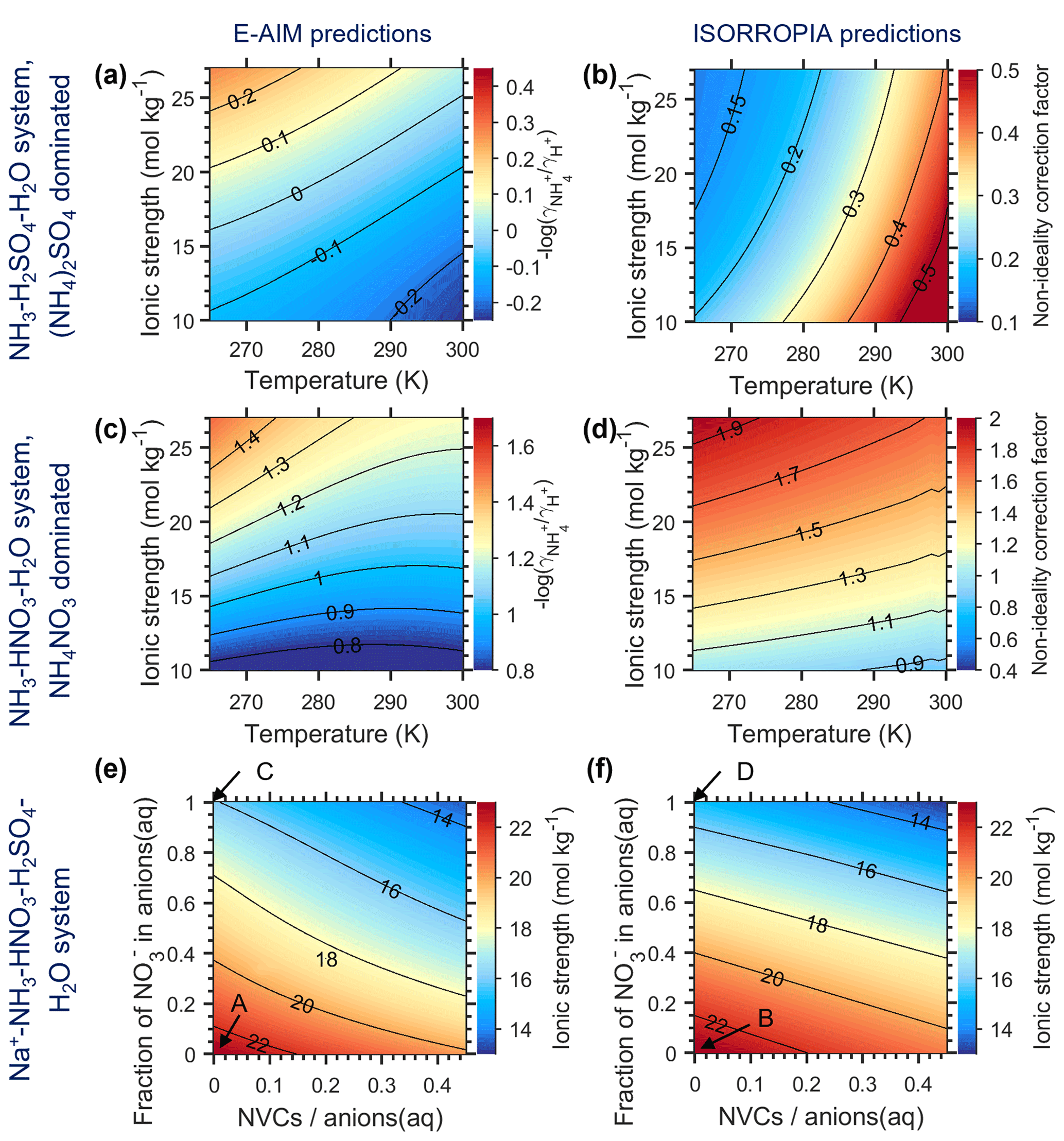
Figure A1Ionic strength (I) and the non-ideality correction factor, cni, as calculated by E-AIM (a, c, e) and ISORROPIA (b, d, f) under different aerosol systems. The systems are the same as in Fig. 1, while the RH in Fig. 1a–d and cni in Fig. 1e–f are replaced by I.
NH3–H2SO4–H2O system. For this system, we assumed a constant input with 0.5 µmol m−3 of total sulfate (i.e., 1 µeq m−3of anions) and 2 µmol m−3 of total ammonia. This ratio is to ensure that the system pH is around the maximum buffering capacity of ammonia. However, we found that for the ISORROPIA model, the solver with only ammonia and sulfate inputs is not stable, with the predicted pH often larger than 7. We thereby introduced 0.015 µmol m−3 of Na+ (3 % of the total sulfate molar concentrations or 1.5 % of the anions), which exerted little influence on the ionic environments (difference in E-AIM results less than 3 %) but will change the ISORROPIA subroutine solver called. The RH and temperature are then varied at different values to check the influence.
NH3–HNO3–H2O system. For this system, we assumed a constant input with 1 µmol m−3 of total nitrate (also 1 µeq m−3of anions) and 2 µmol m−3 of total ammonia and then varied the RH and temperatures to derive non-ideality correction factors.
Na+–NH3–HNO3–H2SO4–H2O system. For this system, we fixed the RH at 73 % and temperature at 288.15 K, 2 µmol m−3 of total ammonia and a fixed concentration of total anions of 1 µeq m−3. The nitrate sulfate ratios are then varied (but keeping their total charges the same) to get different nitrate fractions. For example, when the input sulfate is 0.25 µmol m−3 equalling 0.5 µeq m−3 of anions, the input total nitrate is then set to 0.5 µmol m−3, corresponding to a total anion of the system of 1 µeq m−3. Meanwhile, the ratio of NVCs (here assumed to be Na+ only) to anions is also varied and combined with the different nitrate sulfate ratios to generate different simulation conditions.

Figure B1Dependence of the non-ideality correction factor for activity-based pH definitions, cnia (i.e., −log(), as estimated by E-AIM. (a) NH3–HNO3–H2O system with aerosols dominated by NH4NO3 at varying RH and temperature conditions and (b) Na+–NH3–HNO3–H2SO4–H2O system with varying chemical profiles at 288.15 K and a RH of 73 %. Note that the cnia for the NH3–H2SO4–H2O system (i.e., (NH4)2SO4-dominated aerosols) is not shown, as it varied little (ranging 0.44–0.47) over all the RH and temperature ranges explored.
With an activity-based pH definition (i.e., pH ( [H+]), the multiphase buffer theory can be rewritten as
where is the multiphase effective acid dissociation constant under non-ideal conditions. The difference in pH caused by non-ideality, cnia, is therefore
That is, the non-ideality correction factor for activity-based pH is actually the , which can be calculated with the more comprehensive models like E-AIM. The E-AIM calculated mole-fraction-based activity coefficient (fi) that can be converted to the molality-based activity coefficient (γi) by (Pye et al., 2020; Peng et al., 2019)
where xi and mi are, respectively, the mole fraction and molality of species i and xw and Mw are, respectively, the mole fraction and molecular weight of water. All these variables are given in E-AIM outputs. Major influencing factors of cnia are also RH, temperature and the fraction of NO in anions in the aqueous phase (aq), as shown in Fig. B1.
In this section, we will only focus on the model settings for EMAC simulations, while for the GEOS-chem model settings, please refer to Zheng et al. (2020). We used the global ECHAM/MESSy Atmospheric chemistry – Climate (EMAC) model, which is a numerical chemistry and climate simulation system that includes submodels describing tropospheric and middle-atmosphere processes and their interaction with oceans, land and human influences (Jöckel et al., 2010). The core atmospheric model is the 5th generation European Centre Hamburg general circulation model (ECHAM5) (Roeckner et al., 2006), which has been modularized and which improved submodels and updates of boundary layer, radiation, cloud and convection routines have been introduced. The EMAC model development is coordinated within an international consortium: see https://www.messy-interface.org (last access: 18 November 2021). For the present study we applied EMAC (ECHAM5 version 5.3.02, MESSy version 2.54.0) in the T63L31 resolution, i.e., with a spherical truncation of T63 (corresponding to a quadratic Gaussian grid of approximately 1.8 by 1.8∘ in latitude and longitude) with 31 vertical hybrid terrain-following pressure levels up to 10 hPa in the lower stratosphere. Meteorological conditions as in ERA-Interim data from the European Centre for Medium- range Weather Forecasts (ECMWF) were simulated by the model by applying a “nudging” technique (Jöckel et al., 2006). EMAC simulates gas-phase and heterogeneous chemistry through the MECCA submodel, which accounts for the photochemical oxidation of natural and anthropogenic emissions, including a comprehensive account of volatile organic carbon compounds (Sander et al., 2019). Aerosol microphysical processes and gas–particle partitioning are simulated with the GMXe submodel (Pringle et al., 2010; Pozzer et al., 2012), which describes the aerosol size distribution by seven interacting lognormal modes (four hydrophilic and three hydrophobic). The aerosol composition can vary between these modes (externally mixed) and is uniform within each mode (internally mixed). The inorganic aerosol composition is computed with the ISORROPIA-II thermodynamic equilibrium submodel (Fountoukis and Nenes, 2007). It calculates the gas–liquid–solid equilibrium partitioning of inorganic compounds and water. The composition and atmospheric evolution of organic aerosol compounds is simulated with the ORACLE submodel, which represents volatility classes of organics through their effective saturation concentrations (Tsimpidi et al., 2018). For this work the anthropogenic emissions from EDGAR (Emissions Database for Global Atmospheric Research v4.3.2) (Crippa et al., 2018) were applied, as well as the GFAS (Global Fire Assimilation System, v1.0) (Kaiser et al., 2012) for biomass burning emissions. The EMAC results are shown in Fig. C1.
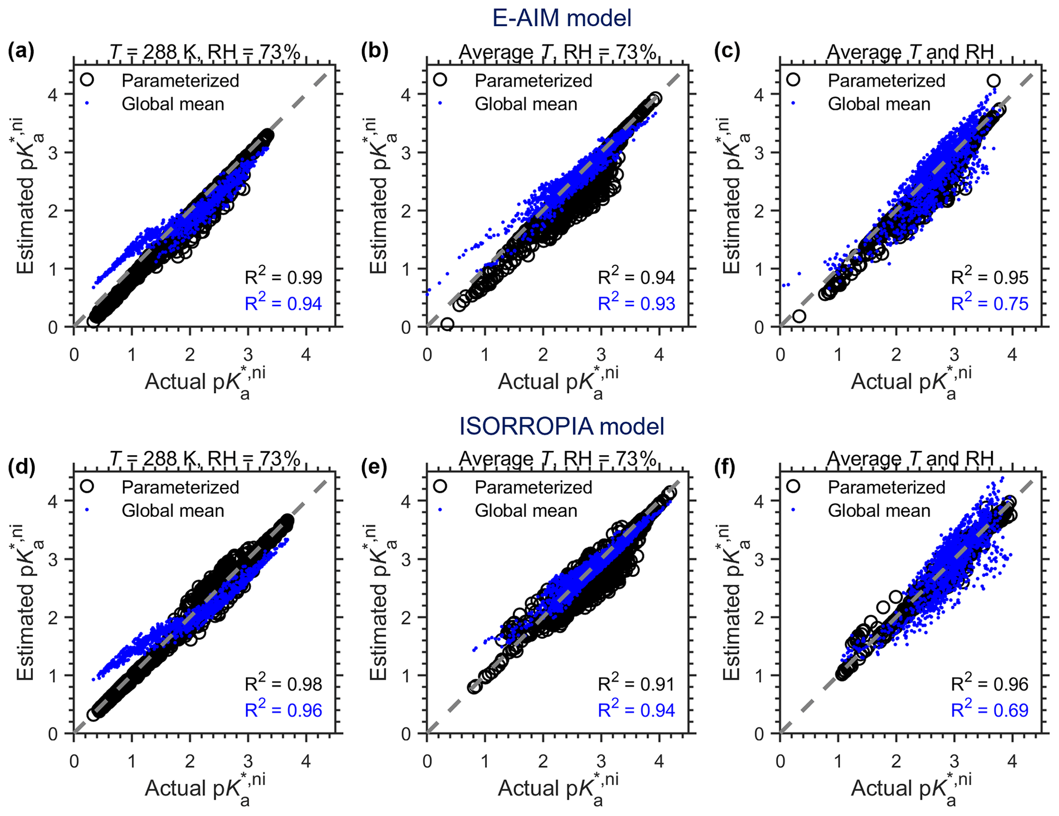
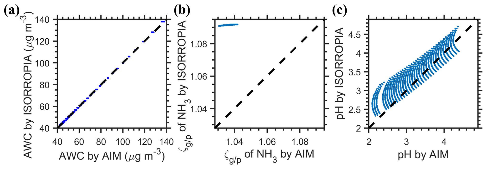
Figure D1Drivers of the difference in cni estimated by the ISORROPIA and E-AIM models for the NH3–H2SO4–H2O system. The of NH3 indicates the molar ratios of NH3(g) to particle-phase NH.
In this study, we applied ISORROPIA version 2.1 (Fountoukis and Nenes, 2007) and E-AIM (model IV; http://www.aim.env.uea.ac.uk/aim/aim.php, last access: 18 November 2021) (Clegg et al., 1992; Wexler and Clegg, 2002; Friese and Ebel, 2010), and the following description and discussion refer to these versions of the models. For the NH3–H2SO4–H2O system, we found that by assuming the same input of 0.5 µmol m−3 of total sulfate (i.e., 1 µeq m−3of anions) and 2 µmol m−3 of total ammonia and varying the RH (60 %–90 %) and temperatures (265–300 K), ISORROPIA predicted a very high aerosol pH of about 13 (12.6–13.2), while the E-AIM-predicted pH ranged from 2–5, which is obviously more realistic. However, by introducing only an small amount of Na+ (0.015 µmol m−3 or 3 % of the total sulfate), the ISORROPIA-predicted pH dropped dramatically to 2–5 (Fig. D1), while the E-AIM-predicted pH changed little compared to the no-Na+ predictions (pH increased systematically by 0.03 with both R2 and slope being 1). Besides, the predicted pH assuming only HNO3 and NH3 inputs (NH3–HNO3–H2O system) agreed well between ISORROPIA and E-AIM.

Figure D2Comparison of activity coefficients for different species. (a–c) Comparison of activity coefficients involved in ISORROPIA A2 subcase calculations, as predicted by ISORROPIA and E-AIM. (d) Comparison of activity coefficients involved in ISORROPIA D3 subcase calculations, as predicted by ISORROPIA and E-AIM. (e) Mean activity coefficients predicted by ISORROPIA that are involved in ISORROPIA G5 subcase calculations.
We found that the dramatic changes in ISORROPIA-predicted pH levels with or without small amounts of Na+ and NO additions are related to the different calculation procedures among subcases. Here we focused on subcases under the metastable and sulfate-poor (i.e., total potential cations, including total ammonia ([NH3]t) and NVCs, exceed twice the molar ratios of total sulfate ([H2SO4]t)) conditions.
In ISORROPIA, when there are only NH3 and H2SO4 (i.e., the “pure” NH3–H2SO4–H2O system), the corresponding subcase is “A2”. As detailed below, for this subcase, activity coefficients included in the final calculations are , and . As shown in Fig. D2a–c, for all these three values, there is a large difference between E-AIM and ISORROPIA estimations (note that log scales are used for and plots). Therefore, it is not surprising that there is a large discrepancy between the predicted pH from subcase A2 of ISORROPIA and E-AIM.
In comparison, the subcase would change to “D3” when HNO3 is introduced to the system. As detailed below, for this subcase, only is involved in the calculations. As shown in Fig. D2d, although ISORROPIA still shows a different trend than E-AIM, it is, however, at least on the same order of magnitude as the one predicted by E-AIM.
By introducing a small amount of Na+ into the NH3–H2SO4–H2O system, the calculation procedure of ISORROPIA would change from A2 to G5 (an Na+–NH3–H2SO4–HNO3–HCl–H2O aerosol system). For the G5 subcase, we noticed two issues: (1) although the total HNO3 is zero, the model still tried to predict and ; (2) as it was using Cl− as the x variable for the final solutions, a small amount of Cl− was always present, which was introduced by the model so the calculation procedures could go on. The relevant values are shown in Fig. D2e. In comparison, E-AIM predicted no NO or Cl−, and the activity coefficients of other relevant species change little with the no-Na+ case. Therefore, we could not perform a comparison between ISORROPIA and E-AIM for this case (as there is no or γCl in E-AIM). Based on the pH and non-ideality comparisons (Fig. D1), however, we could see that the NH3 partitioning estimated in this way is far more realistic than the A2 subcase.
Calculation principles for subcase A2 (an NH3–H2SO4–H2O aerosol system). For the subcase A2, the major constraining equations include the [SO][HSO] equilibriums, gas–particle partitioning of ammonia and charge balance:
With these three equations and known total ammonia ([NH3]t) and total sulfate ([H2SO4]t), we have
where , while . The only unknown is thus [H+], which can thus be solved by bisection solution processes. As shown in the equation, activity coefficients that matter in solving this system include in C1 and in C2S.
Calculation principles for subcase D3 (an NH3–H2SO4–HNO3–H2O aerosol system). For the subcase D3, the major equilibriums considered is the gas–particle partitioning of ammonia and nitrates of
Note that in subcase D3, is estimated by (, not ( as in subcase A2.
These two equilibriums are further combined to be
As to the charge balance, here only major species are regarded as
Combining Eqs. (D5a) and (D5b), at given total nitrate ([HNO3]t, namely [NO(aq)] + [HNO3(g)]) and [NH3]t (= [NH(aq)] + [NH3(g)]) levels, the solution function can be expressed as
where the only unknown is [NH(aq)] and can be solved through the bisection method. As shown in the equation, the only activity coefficient that matters in solving this system is ( in C3.
Calculation principles for subcase G5 (a Na+–NH3–H2SO4–HNO3–HCl–H2O aerosol system). For the subcase G5, the major equilibriums considered are the gas–particle partitioning of NH3, HNO3 and HCl, while sulfate is considered to exist mainly as [SO(aq)]. General derivation processes are similar with D3 and are also detailed in a previous study (Song et al., 2018). Briefly, the key equilibriums include that of HNO3 (Eq. D4) and HCl of
which can be combined into
Therefore [NO (aq)] and [HNO3(g)] (=[HNO3]t − [NO (aq)]) can be solved at known assumed [Cl−(aq)].
The [NH(aq)] associated with Cl−(aq) and NO(aq), [NH(aq)]NC, is solved by
where
where . And with [NH(aq)]NC, we have
The system then solves the equation sets through the bisection method by assuming a series of [Cl−(aq)] levels.
As shown in the equations above, activity coefficients that matter in solving this system (Eqs. D8–D9) include , γH−Cl and .
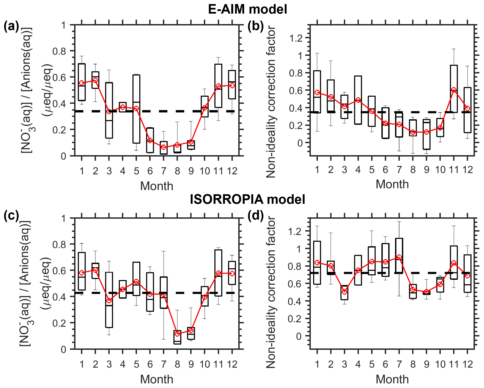
Figure E1Monthly variation in (a, c) NO3- fraction in anions(aq) and (b, d) the corresponding non-ideality correction factors for the Toronto site in 2012. The data are estimated by (a–b) the E-AIM model and (c–d) the ISORROPIA model. The black dash lines represent the annual mean levels. The box and whiskers represent the 10th, 25th, 50th, 75th and 90th percentiles, while the red markers represent the monthly means.
All data used in this study are described in the paper and Supplement.
The supplement related to this article is available online at: https://doi.org/10.5194/acp-22-47-2022-supplement.
YC, HS and GZ designed the study. GZ performed the study. SW provided GEOS-Chem model results. AP provided the global numerical EMAC model results. GZ, YC and HS wrote the paper with input from all coauthors.
The authors declare that they have no conflict of interest.
Publisher's note: Copernicus Publications remains neutral with regard to jurisdictional claims in published maps and institutional affiliations.
The research was supported by the Max Planck Society (MPG). Yafang Cheng acknowledges the Minerva Program of MPG. We would like to thank Ulrich Pöschl for the helpful discussion and support.
The article processing charges for this open-access publication were covered by the Max Planck Society.
This paper was edited by Veli-Matti Kerminen and reviewed by Yunhong Zhang and two anonymous referees.
Ault, A. P.: Aerosol Acidity: Novel Measurements and Implications for Atmospheric Chemistry, Accounts Chem. Res., 53, 1703–1714, https://doi.org/10.1021/acs.accounts.0c00303, 2020.
Clegg, S. L., Pitzer, K. S., and Brimblecombe, P.: Thermodynamics of multicomponent, miscible, ionic-solutions. 2. Mixtures including unsymmetrical electrolytes, J. Phys. Chem., 96, 9470–9479, https://doi.org/10.1021/j100202a074, 1992.
Clegg, S. L., Brimblecombe, P., and Wexler, A. S.: Thermodynamic model of the system H+-NH-Na+-SO-NO-Cl−-H2O at 298.15 K, J. Phys. Chem. A, 102, 2155–2171, https://doi.org/10.1021/jp973043j, 1998.
Clegg, S. L., Seinfeld, J. H., and Brimblecombe, P.: Thermodynamic modelling of aqueous aerosols containing electrolytes and dissolved organic compounds, J. Aerosol Sci., 32, 713–738, https://doi.org/10.1016/S0021-8502(00)00105-1, 2001.
Craig, R. L., Peterson, P. K., Nandy, L., Lei, Z., Hossain, M. A., Camarena, S., Dodson, R. A., Cook, R. D., Dutcher, C. S., and Ault, A. P.: Direct Determination of Aerosol pH: Size-Resolved Measurements of Submicrometer and Supermicrometer Aqueous Particles, Anal. Chem., 90, 11232–11239, https://doi.org/10.1021/acs.analchem.8b00586, 2018.
Crippa, M., Guizzardi, D., Muntean, M., Schaaf, E., Dentener, F., van Aardenne, J. A., Monni, S., Doering, U., Olivier, J. G. J., Pagliari, V., and Janssens-Maenhout, G.: Gridded emissions of air pollutants for the period 1970–2012 within EDGAR v4.3.2, Earth Syst. Sci. Data, 10, 1987–2013, https://doi.org/10.5194/essd-10-1987-2018, 2018.
Fountoukis, C. and Nenes, A.: ISORROPIA II: a computationally efficient thermodynamic equilibrium model for K+–Ca2+–Mg2+––Na+–––Cl−–H2O aerosols, Atmos. Chem. Phys., 7, 4639–4659, https://doi.org/10.5194/acp-7-4639-2007, 2007.
Fountoukis, C., Nenes, A., Sullivan, A., Weber, R., Van Reken, T., Fischer, M., Matías, E., Moya, M., Farmer, D., and Cohen, R. C.: Thermodynamic characterization of Mexico City aerosol during MILAGRO 2006, Atmos. Chem. Phys., 9, 2141–2156, https://doi.org/10.5194/acp-9-2141-2009, 2009.
Friese, E. and Ebel, A.: Temperature Dependent Thermodynamic Model of the System H+-NH-Na+-SO-NO-Cl−-H2O, J. Phys. Chem. A, 114, 11595–11631, https://doi.org/10.1021/jp101041j, 2010.
Guo, H., Xu, L., Bougiatioti, A., Cerully, K. M., Capps, S. L., Hite Jr., J. R., Carlton, A. G., Lee, S.-H., Bergin, M. H., Ng, N. L., Nenes, A., and Weber, R. J.: Fine-particle water and pH in the southeastern United States, Atmos. Chem. Phys., 15, 5211–5228, https://doi.org/10.5194/acp-15-5211-2015, 2015.
Guo, H., Sullivan, A. P., Campuzano-Jost, P., Schroder, J. C., Lopez-Hilfiker, F. D., Dibb, J. E., Jimenez, J. L., Thornton, J. A., Brown, S. S., Nenes, A., and Weber, R. J.: Fine particle pH and the partitioning of nitric acid during winter in the northeastern United States, J. Geophys. Res.-Atmos., 121, 10355–310376, https://doi.org/10.1002/2016JD025311, 2016.
Guo, H., Nenes, A., and Weber, R. J.: The underappreciated role of nonvolatile cations in aerosol ammonium-sulfate molar ratios, Atmos. Chem. Phys., 18, 17307–17323, https://doi.org/10.5194/acp-18-17307-2018, 2018.
Hennigan, C. J., Izumi, J., Sullivan, A. P., Weber, R. J., and Nenes, A.: A critical evaluation of proxy methods used to estimate the acidity of atmospheric particles, Atmos. Chem. Phys., 15, 2775–2790, https://doi.org/10.5194/acp-15-2775-2015, 2015.
Jöckel, P., Tost, H., Pozzer, A., Brühl, C., Buchholz, J., Ganzeveld, L., Hoor, P., Kerkweg, A., Lawrence, M. G., Sander, R., Steil, B., Stiller, G., Tanarhte, M., Taraborrelli, D., van Aardenne, J., and Lelieveld, J.: The atmospheric chemistry general circulation model ECHAM5/MESSy1: consistent simulation of ozone from the surface to the mesosphere, Atmos. Chem. Phys., 6, 5067–5104, https://doi.org/10.5194/acp-6-5067-2006, 2006.
Jöckel, P., Kerkweg, A., Pozzer, A., Sander, R., Tost, H., Riede, H., Baumgaertner, A., Gromov, S., and Kern, B.: Development cycle 2 of the Modular Earth Submodel System (MESSy2), Geosci. Model Dev., 3, 717–752, https://doi.org/10.5194/gmd-3-717-2010, 2010.
Kaiser, J. W., Heil, A., Andreae, M. O., Benedetti, A., Chubarova, N., Jones, L., Morcrette, J.-J., Razinger, M., Schultz, M. G., Suttie, M., and van der Werf, G. R.: Biomass burning emissions estimated with a global fire assimilation system based on observed fire radiative power, Biogeosciences, 9, 527–554, https://doi.org/10.5194/bg-9-527-2012, 2012.
Li, G., Su, H., Ma, N., Zheng, G., Kuhn, U., Li, M., Klimach, T., Pöschl, U., and Cheng, Y.: Multifactor colorimetric analysis on pH-indicator papers: an optimized approach for direct determination of ambient aerosol pH, Atmos. Meas. Tech., 13, 6053–6065, https://doi.org/10.5194/amt-13-6053-2020, 2020.
Nenes, A., Pandis, S. N., Weber, R. J., and Russell, A.: Aerosol pH and liquid water content determine when particulate matter is sensitive to ammonia and nitrate availability, Atmos. Chem. Phys., 20, 3249–3258, https://doi.org/10.5194/acp-20-3249-2020, 2020.
Peng, X., Vasilakos, P., Nenes, A., Shi, G., Qian, Y., Shi, X., Xiao, Z., Chen, K., Feng, Y., and Russell, A. G.: Detailed Analysis of Estimated pH, Activity Coefficients, and Ion Concentrations between the Three Aerosol Thermodynamic Models, Environ. Sci. Technol., 53, 8903–8913, https://doi.org/10.1021/acs.est.9b00181, 2019.
Pfennig, B. W.: Principles of inorganic chemistry, John Wiley & Sons, 2015.
Pozzer, A., de Meij, A., Pringle, K. J., Tost, H., Doering, U. M., van Aardenne, J., and Lelieveld, J.: Distributions and regional budgets of aerosols and their precursors simulated with the EMAC chemistry-climate model, Atmos. Chem. Phys., 12, 961–987, https://doi.org/10.5194/acp-12-961-2012, 2012.
Pringle, K. J., Tost, H., Message, S., Steil, B., Giannadaki, D., Nenes, A., Fountoukis, C., Stier, P., Vignati, E., and Lelieveld, J.: Description and evaluation of GMXe: a new aerosol submodel for global simulations (v1), Geosci. Model Dev., 3, 391–412, https://doi.org/10.5194/gmd-3-391-2010, 2010.
Pye, H. O. T., Zuend, A., Fry, J. L., Isaacman-VanWertz, G., Capps, S. L., Appel, K. W., Foroutan, H., Xu, L., Ng, N. L., and Goldstein, A. H.: Coupling of organic and inorganic aerosol systems and the effect on gas–particle partitioning in the southeastern US, Atmos. Chem. Phys., 18, 357–370, https://doi.org/10.5194/acp-18-357-2018, 2018.
Pye, H. O. T., Nenes, A., Alexander, B., Ault, A. P., Barth, M. C., Clegg, S. L., Collett Jr., J. L., Fahey, K. M., Hennigan, C. J., Herrmann, H., Kanakidou, M., Kelly, J. T., Ku, I.-T., McNeill, V. F., Riemer, N., Schaefer, T., Shi, G., Tilgner, A., Walker, J. T., Wang, T., Weber, R., Xing, J., Zaveri, R. A., and Zuend, A.: The acidity of atmospheric particles and clouds, Atmos. Chem. Phys., 20, 4809–4888, https://doi.org/10.5194/acp-20-4809-2020, 2020.
Roeckner, E., Brokopf, R., Esch, M., Giorgetta, M., Hagemann, S., Kornblueh, L., Manzini, E., Schlese, U., and Schulzweida, U.: Sensitivity of Simulated Climate to Horizontal and Vertical Resolution in the ECHAM5 Atmosphere Model, J. Climate, 19, 3771–3791, https://doi.org/10.1175/jcli3824.1, 2006.
Sander, R., Baumgaertner, A., Cabrera-Perez, D., Frank, F., Gromov, S., Grooß, J.-U., Harder, H., Huijnen, V., Jöckel, P., Karydis, V. A., Niemeyer, K. E., Pozzer, A., Riede, H., Schultz, M. G., Taraborrelli, D., and Tauer, S.: The community atmospheric chemistry box model CAABA/MECCA-4.0, Geosci. Model Dev., 12, 1365–1385, https://doi.org/10.5194/gmd-12-1365-2019, 2019.
Song, S., Gao, M., Xu, W., Shao, J., Shi, G., Wang, S., Wang, Y., Sun, Y., and McElroy, M. B.: Fine-particle pH for Beijing winter haze as inferred from different thermodynamic equilibrium models, Atmos. Chem. Phys., 18, 7423–7438, https://doi.org/10.5194/acp-18-7423-2018, 2018.
Tao, Y. and Murphy, J. G.: The sensitivity of PM2.5 acidity to meteorological parameters and chemical composition changes: 10-year records from six Canadian monitoring sites, Atmos. Chem. Phys., 19, 9309–9320, https://doi.org/10.5194/acp-19-9309-2019, 2019.
Tsimpidi, A. P., Karydis, V. A., Pozzer, A., Pandis, S. N., and Lelieveld, J.: ORACLE 2-D (v2.0): an efficient module to compute the volatility and oxygen content of organic aerosol with a global chemistry–climate model, Geosci. Model Dev., 11, 3369–3389, https://doi.org/10.5194/gmd-11-3369-2018, 2018.
Weber, R. J., Guo, H., Russell, A. G., and Nenes, A.: High aerosol acidity despite declining atmospheric sulfate concentrations over the past 15 years, Nat. Geosci., 9, 282-285, https://doi.org/10.1038/ngeo2665, 2016.
Wei, H., Vejerano, E. P., Leng, W., Huang, Q., Willner, M. R., Marr, L. C., and Vikesland, P. J.: Aerosol microdroplets exhibit a stable pH gradient, P. Natl. Acad. Sci. USA, 115, 7272–7277, https://doi.org/10.1073/pnas.1720488115, 2018.
Wexler, A. S. and Clegg, S. L.: Atmospheric aerosol models for systems including the ions H+, NH, Na+, SO, NO, Cl−, Br−, and H2O, J. Geophys. Res.-Atmos., 107, ACH 14-11–ACH 14-14, https://doi.org/10.1029/2001jd000451, 2002.
Zaveri, R. A., Easter, R. C., and Wexler, A. S.: A new method for multicomponent activity coefficients of electrolytes in aqueous atmospheric aerosols, J. Geophys. Res.-Atmos., 110, D12311, https://doi.org/10.1029/2004jd004681, 2005.
Zheng, G., Su, H., Wang, S., Andreae, M. O., Pöschl, U., and Cheng, Y.: Multiphase buffer theory explains contrasts in atmospheric aerosol acidity, Science, 369, 1374–1377, https://doi.org/10.1126/science.aba3719, 2020.
Zuend, A., Marcolli, C., Luo, B. P., and Peter, T.: A thermodynamic model of mixed organic-inorganic aerosols to predict activity coefficients, Atmos. Chem. Phys., 8, 4559–4593, https://doi.org/10.5194/acp-8-4559-2008, 2008.
- Abstract
- Introduction
- Methods
- Results and discussion
- Conclusions
- Appendix A: Scenario settings for different systems
- Appendix B: Non-ideality correction factor for activity-based pH definitions
- Appendix C: EMAC model settings
- Appendix D: Potential reasons for discrepancies in predicting aerosol pH by ISORROPIA and E-AIM for the NH3–H2SO4–H2O system
- Appendix E: Information for the assumed calibration year of 2012 in Toronto site (Fig. E1).
- Data availability
- Author contributions
- Competing interests
- Disclaimer
- Acknowledgements
- Financial support
- Review statement
- References
- Supplement