the Creative Commons Attribution 4.0 License.
the Creative Commons Attribution 4.0 License.
 | 08 Apr 2022
Impacts of three types of solar geoengineering on the Atlantic Meridional Overturning Circulation
Mengdie Xie
John C. Moore
Liyun Zhao
Michael Wolovick
Helene Muri
Climate models simulate lower rates of North Atlantic heat transport under greenhouse gas climates than at present due to a reduction in the strength of the Atlantic Meridional Overturning Circulation (AMOC). Solar geoengineering whereby surface temperatures are cooled by reduction of incoming shortwave radiation may be expected to ameliorate this effect. We investigate this using six Earth system models running scenarios from GeoMIP (Geoengineering Model Intercomparison Project) in the cases of (i) reduction in the solar constant, mimicking dimming of the sun; (ii) sulfate aerosol injection into the lower equatorial stratosphere; and (iii) brightening of the ocean regions, mimicking enhancing tropospheric cloud amounts. We find that despite across-model differences, AMOC decreases are attributable to reduced air–ocean temperature differences and reduced September Arctic sea ice extent, with no significant impact from changing surface winds or precipitation − evaporation. Reversing the surface freshening of the North Atlantic overturning regions caused by decreased summer sea ice sea helps to promote AMOC. When comparing the geoengineering types after normalizing them for the differences in top-of-atmosphere radiative forcing, we find that solar dimming is more effective than either marine cloud brightening or stratospheric aerosol injection.
- Article
(3788 KB) - Full-text XML
-
Supplement
(2837 KB) - BibTeX
- EndNote


Geoengineering, i.e., the deliberate and large-scale manipulation of the Earth's climate, has been proposed as a way to mitigate or offset some of the impacts of anthropogenic global warming (Keith, 2000). Solar radiation management (SRM) is one of the fundamental geoengineering methodologies, increasing Earth's albedo to reduce the net solar irradiance reaching Earth, thus balancing longwave greenhouse gas (GHG) forcing (Niemeier et al., 2013). Stratospheric aerosol injection (SAI), whereby aerosols aloft reflect incoming solar radiation, and marine cloud brightening (MCB), i.e., introducing aerosols into the marine boundary layer and thereby increasing cloud droplet numbers and hence their reflectivity (Jones et al., 2011; Ahlm et al., 2017), are the most commonly discussed methods. Another hypothesized method of SRM is simply blocking some incoming solar radiation before it reaches the Earth (Angel, 2006), known as solar dimming or sunshade geoengineering, and it has proven useful because of the climate response insights it provides. All three methods can cool global mean temperatures, but the tropospheric marine injection in MCB produces greater disparity in regional climate effects, such as on precipitation (Muri et al., 2018; Kravitz et al., 2018). This is not necessarily an inherent disadvantage relative to SAI since it is plausible that combining different SRM methods may deal with regionally specific deleterious impacts of climate change better than any one method alone (Cao et al., 2017).
The most comprehensive model simulations of climate under SRM scenarios to date come from the GeoMIP (Geoengineering Model Intercomparison Project; Kravitz et al., 2013, 2016). These experiments are highly idealized – for example, offsetting of a sudden quadrupling of CO2 concentrations by turning down the solar constant. The point of the experiments is to examine the mechanistic behavior of the climate system when subjected to different styles of SRM forcing in comparison to pure greenhouse gas (GHG) forcing. The global nature of the scenarios allows for sufficient signal-to-noise ratio to discern impacts on various parts of the climate system in a reasonable simulation period with Earth system models (ESMs). There are still technical barriers and risks to doing both MCB (Latham et al., 2012) and SAI (Smith and Wagner, 2018), while doing sunshade SRM is well beyond the bounds of likelihood (Angel, 2006). We are not advocating implementation anytime soon. Instead, our aim with this paper is to use the GeoMIP experiments to investigate the mechanistic effect that SRM and MCB has on an important and unique climate subsystem: the Atlantic Meridional Overturning Circulation (AMOC).
The AMOC describes an ocean circulation that is highly correlated with the poleward transport of heat in the subtropical North Atlantic (Johns et al., 2011). AMOC transports 90 % of the ocean meridional heat at 26.5∘ N (Johns et al., 2011). The upper branch of AMOC transports warm surface freshwater from the tropics northward where it loses heat, densifies and eventually descends in the North Atlantic deep convection regions. AMOC releases about 1.25 PW of heat from the sea to the atmosphere between 26 and 50∘ N, which warms the North Atlantic region and northern Europe, while the deep branch transports cold salty deep water southward that ultimately fills a large fraction of the global ocean basins (Buckley and Marshall, 2016; Chen and Tung, 2018). AMOC is mainly driven by global density gradients due to surface heat and freshwater fluxes (more details are available in McCarthy et al., 2019). Its potential for net northward heat transport is unique and plays an essential role in global climate and the redistribution of heat. Changes to the heat and salt fluxes carried by AMOC must produce various climatic effects, such as changes in tropical cyclone number and intensity (and hence hurricanes impacting its western boundaries) and changes in monsoonal rainfall in Africa and India (Buckley and Marshall, 2016). Therefore, any effects that SRM may have on AMOC have the potential to produce wide-ranging, societally relevant consequences.
It has proven very difficult to observe the magnitude of AMOC directly (McCarthy et al., 2019; Send et al., 2011), so the observational evidence for AMOC strength remains limited. It has been possible to accurately quantify the temporal variation of AMOC only since April 2004, when continuous observations of AMOC began at 26.5∘ N by the Rapid Climate Change–Meridional Overturning Circulation and Heat flux Array–Western Boundary Time Series (RAPID–MOCHA–WBTS) project in the North Atlantic (Smeed et al., 2018). The mean strength of AMOC from April 2004 to February 2017 was 17.0 Sv (sverdrup) with a standard deviation of 4.4 Sv (Frajka-Williams et al., 2019). The 26.5∘ N array observations provide information on the short-term interannual and seasonal variability of AMOC. Annually, AMOC ranges in strength from 4 to 35 Sv and also has seasonal characteristics (Frajka-Williams et al., 2019). AMOC intensity decreased significantly during 2004–2012 but was then statistically unchanged between 2012 and 2017 (Smeed et al., 2018). The decline is thought to be related to the Atlantic Multidecadal Oscillation and not to the long-term external climate forcing. The less than two-decade observational record is insufficient to detect the effect of external climate stress on AMOC (Roberts et al., 2014). Numerical climate models show a slight decline of AMOC in the historical period and predict that AMOC will continue to weaken in the 21st century (Cheng et al., 2013). Predicted AMOC decline is stronger in more recent models than in earlier ones, with modern ensemble mean estimates suggesting declines between 6 and 8 Sv (34 %–45 %) by 2100 (Weijer et al., 2020). Compared to the past 1500 years, AMOC has experienced an exceptional weakening in the past 150 years (Thornalley et al., 2018).
The external forcing factors that control AMOC intensity depend on the timescale being considered. On short timescales (monthly to seasonal), change in wind stress can be the main factor affecting its intensity (Zhao and Johns, 2014), but on long timescales (interannual to interdecadal) the seawater density affected by freshwater flux and sea–air heat flux are the main factors (Smeed et al., 2018).
To date, little research on the oceanic response at high northern latitudes under SRM has been published (Malik et al., 2020; Muri et al., 2018; Smyth et al., 2017). Some research has been done on AMOC under sunshade geoengineering (Hong et al., 2017) and under SAI (Muri et al., 2018; Moore et al., 2019; Tilmes et al., 2020). As with GHG forcing alone, these studies found a weakening of AMOC relative to the present day under sunshade geoengineering, mainly in response to the change of heat flux in the North Atlantic, with little influence from the changes of freshwater flux and wind stress (Hong et al., 2017). However, the AMOC is less weakened under sunshade geoengineering than with GHG forcing alone (Hong et al., 2017). Under SAI experiments, AMOC declines seen under greenhouse forcing are consistently reversed (Moore et al., 2019; Tilmes et al., 2020; Muri et al., 2018). All ESM simulation results agree that SAI mitigates weakening of the AMOC as compared to the GHG control experiments. Hence AMOC is closer to the present day with sunshade and SAI SRM than without, but very little research on AMOC under MCB experiments has yet been published (Muri et al., 2018).
Here, we evaluate and compare the potential for MCB to offset changes under GHG forcing to AMOC and its effectiveness and mechanistic behavior relative to SAI and sunshade geoengineering based on the same six ESMs (Table 1). We focus on the response of northward ocean heat transport, freshwater flux, sea–air heat flux, the AMOC strength, atmospheric wind stresses and Arctic sea ice extent.
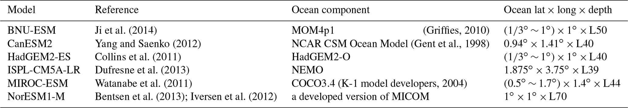
We analyze monthly output from all ESMs that participated in GeoMIP with sufficient data fields available (Table 1). The G1 and G1oceanAlbedo experiments are very idealized simulations where incoming solar radiation is reduced to balance the longwave radiative forcing of quadrupled CO2 relative to preindustrial concentrations. The G4 and G4cdnc experiments represent somewhat more real-world scenarios where the background greenhouse concentration rises as specified by the RCP4.5 scenario (Representative Concentration Pathway), while SRM is prescribed either by constant amounts for SAI (G4) or increased cloud condensation nuclei over the ocean (G4cdnc; see Sect. 2.1 for more information and Kravitz et al., 2011, 2013, for a full description of the experiment design). Hence there are three control simulations: (i) the standard piControl specifying preindustrial conditions, (ii) abrupt4×CO2 specifying the standard abrupt quadrupling of CO2 and (iii) the RCP4.5 scenario specified under the Climate Model Intercomparison Project Phase 5 (CMIP5; Taylor et al., 2012). Not all the ESMs we use have every simulated climate field that we would like; some lack heat and water flux data or sea ice extents (Table S1 in the Supplement).
The response of the oceans is expected to be much slower than the atmosphere. Typically, in the sunshade experiments which invoke abrupt and strong forcing, the first decade of the simulations has not been included in the analysis to mitigate this issue. It is of course unlikely that the deep ocean would be close to a steady state within centuries of beginning geoengineering experiments, but to be practical we assume that the scenario responses after the first decade are sufficiently different from each other to explore impacts. Most GeoMIP scenarios run for 50 years; while some GHG and control scenarios run longer, we limit the analysis of all scenarios to the same duration for statistical convenience. We test for significance at the 95 % level using the nonparametric Wilcoxon signed-rank test.
2.1 Experiments
Schematic representations of the experiments are shown in Fig. 1 and Table 2. G1oceanAlbedo is part of the phase-2 GeoMIP experiments (Kravitz et al., 2013, 2015) and designed to mimic the G1 solar dimming experiment (Kravitz et al., 2011). Both are based on the CMIP5 abrupt4×CO2 experiment and started from a stable preindustrial climate run, i.e., the CMIP5 experiment piControl (Taylor et al., 2012). In the G1 experiment, the radiative forcing from an abrupt quadrupling of CO2 concentrations above preindustrial levels is offset by a uniform insolation reduction, thereby mimicking sunshade geoengineering. In G1oceanAlbedo, the radiative forcing from abrupt4×CO2 is instead compensated for by using a uniform increase in albedo in the ESM ocean-covered grid cells (Fig. 1a). The G4 experiment, by contrast, starts with the RCP4.5 scenario as a baseline and then employs an injection rate of SAI (5 Tg of SO2 per year) into the equatorial lower stratosphere between the years 2020 and 2069 (Fig. 1c). The G4cdnc scenario is similar, except that the stratospheric aerosols are replaced by a 50 % increase in the cloud number droplet concentration in low clouds over the global ice-free oceans. In both G4 and G4cdnc, the amount of geoengineering is held fixed over time rather than being adjusted to balance the radiative forcing due to GHGs.
Table 2A summary of the four experiments included in this proposal.

In the following analysis, we make comparisons between G1oa and G1 and between G4 and G4cdnc separately as they do not use the same greenhouse gas forcing backgrounds (Table 2). But we are also interested in comparing the different geoengineering types, and doing this can be done with the ratios of their response, e.g., (G4-RCP4.5)(G1-Abrupt4×CO2). The different ESMs also have different climate sensitivities, and we also account for this by considering their top-of-atmosphere (TOA) radiative forcing.
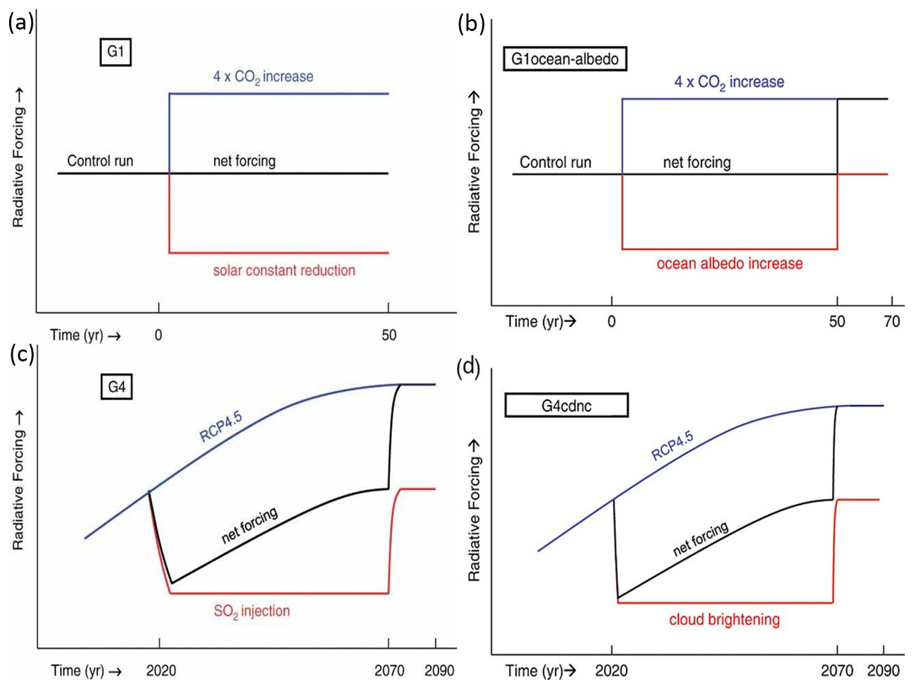
Figure 1Schematics of the four experiments outlined in this paper, based on Kravitz et al. (2011, 2013). (a) G1 is started from a preindustrial control run; longwave forcing (blue) from quadrupled GHG forcing is compensated by a fixed reduction in the solar constant (red) to leave net zero forcing (black); the experiment is for 50 years duration. (b) In G1oceanAlbedo the equivalent balance is obtained by an increase in ocean albedo. (c) G4 is started from 2020 and ends in 2069, branching from RCP4.5 with 5 Tg yr−1 SO2 injected into the equatorial lower stratosphere. (d) In G4cdnc the shortwave forcing comes from a constant 50 % increase in cloud droplet number concentration in oceanic low clouds.
2.2 AMOC index
The AMOC index (Cheng et al., 2013) is defined as the annual-mean maximum volume of the transport stream function at 30∘ N in the North Atlantic (in sverdrup (Sv)). The transport stream function is described by the integral of the meridional transport from the surface to the bottom depth at the given latitude (here 30∘ N):
where Ψ is the overall transport stream function, z is the bottom depth, lat is latitude, and λE and λW represent the eastern and western meridians, respectively. V is the meridional ocean velocity.
2.3 Northward heat transport
In this study, we use the ocean potential temperature and the ocean meridional velocity to calculate the northward heat transport, H (Stouffer et al., 2017):
where H(lat) is the ocean heat transport in the latitude, Cp is the ocean specific heat capacity, ρ is the ocean potential density, long is longitude and T is ocean potential temperature.
3.1 Experiments
Table 3Differences in average AMOC index, upward heat flux (W m−2), September sea ice extent (106 km2) and top-of-atmosphere radiation (W m−2) over the 40-year analysis period. Bold entries denote differences significant at the 95 % level in the Wilcoxon signed-rank test. G1oa refers to G1oceanAlbedo, and piC refers to piControl. Individual ESM results are shown in Tables S2–S5.
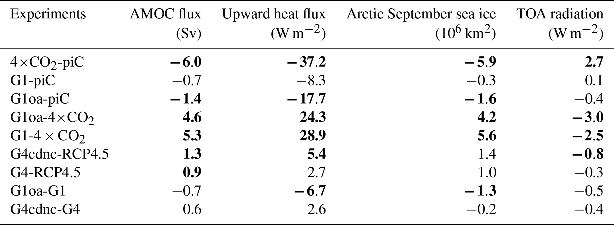
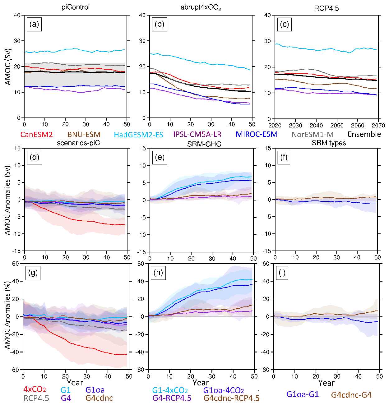
Figure 2The 11-year running annual means simulated by the six ESMs and the multimodel ensemble mean (black curve) of the AMOC strength (Sv) over the 40-year analysis period under (a) piControl, (b) abrupt4×CO2 and (c) RCP4.5. The gray band in (a) is the range of AMOC intensity (17.0 ± 4.4 Sv) measured by the RAPID- MOCHA (Frajka-Williams et al., 2019). Panels (d)–(f) show AMOC anomalies (Sv), and panels (g)–(i) show the percentage changes relative to the other scenarios: left column (d, g) relative to piControl; middle (e, h) relative to global warming scenarios (RCP4.5 and abrupt4×CO2); right (f, i) relative to other geoengineering scenarios (G1oa-G1; G4cdnc-G4). Colored bands in panels (d)–(i) represent the across-ESM spread. G1oa refers to G1oceanAlbedo, and piC refers to piControl.
Under the piControl scenario, the six ESM ensemble mean AMOC index is about 17.9 Sv, which is consistent with the average AMOC strength (17.7 ± 0.3 Sv) from the RAPID- MOCHA array (Weijer et al., 2020) (Fig. 2a). Under RCP4.5, the AMOC intensity decreases by about 2.4 Sv from 2020 to 2069 (Fig. 2c; Table 3), consistent with previously published ESM simulation results (Cheng et al., 2013; Weijer et al., 2020; Muri et al., 2018). Compared to piControl, the AMOC intensity in the 50th year of abrupt4×CO2 decreased by about 7.9 Sv (42 %) compared to a 15 % reduction under RCP4.5 (Fig. 2g), which is consistent with the lower GHG forcing under RCP4.5.
Under G1 and G1oceanAlbedo scenarios, the average AMOC strength over the 40-year analysis period increased by about 5.3 and 4.6 Sv relative to abrupt4×CO2 (Table 3). Compared to abrupt4×CO2, the AMOC intensity in the 50th year of G1 and G1oceanAlbedo increased by about 7.2 Sv (41 %) and 6.2 Sv (35 %) (Fig. 2e, h). The average AMOC intensity is insignificantly weaker under G1 but statistically significant and lower by 1.4 Sv under G1oceanAlbedo (p<0.05; Table 3) than under piControl. MIROC-ESM simulated a slightly stronger AMOC under G1oceanAlbedo than under G1 (Table S2), but the other five ESMs and the ensemble mean agree that AMOC under the G1 scenario is stronger than that under G1oceanAlbedo. Even though G1oceanAlbedo is designed to produce radiative forcing over ice-free oceans, it is significantly less effective at restoring AMOC to piControl levels than the global forcing applied under G1.
Both G4cdnc and G4 apply constant reductions to shortwave solar radiation, but in contrast with the abrupt4×CO2 scenario, the GHG concentrations continue to rise in these scenarios as specified by RCP4.5. Under the G4 and G4cdnc scenarios, the average AMOC strength over the 40-year analysis period increased by about 0.9 and 1.3 Sv relative to RCP4.5 (Table 3), both significantly different from RCP4.5 (Table 3). Five ESMs and the ensemble mean agree that the ocean-only forcing under G4cdnc is more effective than the global G4 forcing for restoring AMOC to present-day strength (Table S2).
We may thus conclude that the four geoengineering experiments mitigate AMOC weakening caused by the forcing of GHG, but the mitigation efficacies are different. Generally, mitigation of AMOC weakening under G4cdnc is more than with G4 but weaker than G1 solar dimming. G1oceanAlbedo is more effective than G4cdnc, but these scenarios were not designed to have identical forcing, so we shall discuss their relative efficacy later in the Discussion section.
3.2 Northward heat transport response
AMOC transports heat from low latitudes to high latitudes at the upper levels of the ocean. How will the northward heat transport change with the change of AMOC intensity under different styles of SRM?

Figure 3Meridional distribution of the average northward heat transport (PW) over the 40-year analysis period at Atlantic Ocean (depth 0–700 m) under (a) piControl, (b) abrupt4×CO2, and (c) RCP4.5. Panels (d)–(f) show northward heat transport anomalies relative to the other scenarios: left column (d) relative to piControl; middle (e) relative to global warming scenarios; right (f) relative to other geoengineering scenarios. Colored bands in panels (d)–(f) represent the across-ESM spread.
Under piControl, the six ESMs ensemble mean northward heat transport at 26.5∘ N in the Atlantic Ocean is about 1.27 PW (Fig. 3a), which is consistent with the estimate by Johns et al. (2011) of 1.25 PW for meridional heat transport in the Atlantic Ocean from 2004 to 2007.
Under the two global warming scenarios (RCP4.5 and 4×CO2), the northward heat transport at the Atlantic basin to the south of 60∘ N decreases significantly relative to piControl, particularly between 30 and 50∘ N, and increases between 60 and 70∘ N (Fig 3d). Under the abrupt4×CO2 and RCP4.5 scenarios, AMOC weakening reduces the heat transported northward by about 0.51 and 0.07 PW between 30 and 50∘ N relative to piControl.
Under G1 and G1oceanAlbedo scenarios, the northward heat transport increased by about 0.45 and 0.4 PW between 30 and 50∘ N relative to abrupt4×CO2 (Fig. 3e). The northward heat transport weakening between 30 and 50∘ N caused by GHGs is significantly mitigated by G1 and G1oceanAlbedo, but the northward heat transport between 30 and 50∘ N is still weaker by about 0.06 and 0.12 PW under G1 and G1oceanAlbedo than under piControl (Fig. 3d). The mitigation of northward heat transport weakening is consistent with the mitigation of AMOC weakening under G1 and G1oceanAlbedo. Northward heat transport weakening between 30 with 50∘ N caused by abrupt4×CO2 is more balanced under G1 than with G1oceanAlbedo, consistent with their relative AMOC performance.
Both G4 and G4cdnc significantly mitigate the reduction of northward heat transport between 30 and 50∘ N in the North Atlantic basin under RCP4.5 (Fig. 3e). Compared to the RCP4.5 scenario, the G4 and G4cdnc scenarios increase the northward heat transport by about 0.1 and 0.08 PW between 30 and 50∘ N. The mitigation of northward heat transport weakening between 30 and 50∘ N is stronger under G4 than G4cdnc, although differences between G4 and G4cdnc are generally not significant at the 95 % level. Changes in northward heat transport are thus more complex than their AMOC responses summarized in Table 3.
Three drivers of AMOC intensity change have been proposed: (i) wind stress at monthly to seasonal periods (Zhao and Johns, 2014) and at annual and decadal scales, (ii) changes in seawater density due to varying freshwater flux, and also (iii) changes in ocean–air heat exchange (Smeed et al., 2018). We consider each of these in relation to the different SRM experiments. We also look at how model dependent the drivers are.
4.1 Near-surface wind speed
We used six ESMs to calculate near-surface wind speed and wind direction under different scenarios. Under the abrupt4×CO2 scenario, the global wind speed has obvious changes compared to other scenarios, especially in the Southern Ocean subpolar westerlies (Fig. 4a). But there is no significant change of wind speed under other scenarios in the Atlantic high latitudes.
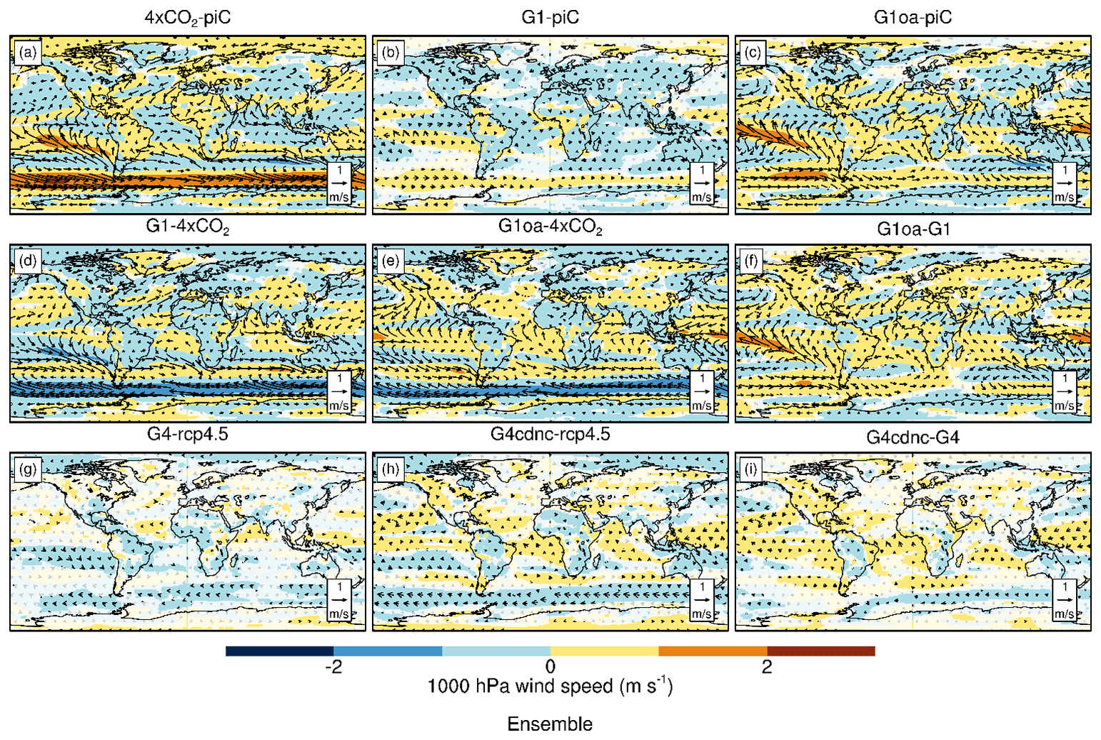
Figure 4Spatial distribution of six ESMs and ensemble mean 1000 hPa wind speed and wind direction (arrows) changes under different scenarios (11–50 years). Blue colors indicate decreased wind speed; the length of arrow in each panel's bottom right represents speeds of 1 m s−1. Translucent white overlay indicates regions where differences are not significant at the 95 % level according to the Wilcoxon signed-rank test.
There is a significant correlation between wind and AMOC when all models and scenarios except for HadGEM2-ES are selected (Fig. 5). AMOC intensity is significantly related to wind speed within the same scenario, as clearly shown for abrupt4×CO2 in red in Fig. 5, which lies on a relation parallel to, but above, the other scenarios. Similarly, for G1 and piControl points lie on a relation parallel to (but lower than) the mean regression. Similar results were obtained for winds only over the deep convection regions and for just the Atlantic north of 45∘ N (Fig. S2). This suggests that the wind speed is correlated with scenario as well as AMOC, but this analysis does not address causal relation between wind and AMOC. This is consistent with the observation that while wind stress clearly affects AMOC on short timescales it is not the main factor affecting AMOC intensity one long timescales (Zhao and Johns, 2014).
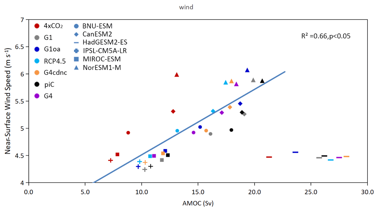
Figure 5ESM mean of wind speed (m s−1) over the 40-year analysis period in the whole North Atlantic (north of 30∘ S). All ESMs except HadGEM2-ES show a high correlation between near-surface wind speed and AMOC intensity. The solid line is the linear regression line of AMOC intensity and wind speed (area average of the whole North Atlantic) over the 40-year analysis period in the five ESMs excluding HadGEM2-ES.
4.2 Upward heat flux
AMOC transports heat from the tropics to high latitudes, releases heat in the deep convective regions of the North Atlantic, and then the surface water density increases and sinks to form cold water flowing southward. Under abrupt4×CO2 and RCP4.5 scenarios, GHG forcing reduces the temperature difference between ocean and atmosphere at high latitudes (Fig. 6b, c), resulting in reduced heat transfer from the ocean to the atmosphere in the deep convective regions (Fig. 7d). The reduction of upward heat flux impedes the release of heat from the seawater, weakening the densification process and the rate of sinking in the deep convective region and thus weakening AMOC.
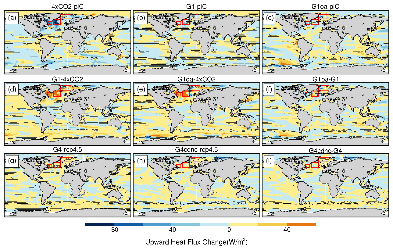
Figure 6Upward heat flux change (W m−2) in different scenarios (11–50 years). The red boxes mark the three deep convective regions in the northern North Atlantic (from left to right: Labrador Sea, Irminger Sea and Nordic Seas (often referred to as the Greenland–Iceland–Norwegian (GIN) Seas). Yellow to orange colors represent an increase in heat flux from the ocean to the atmosphere. Stippling indicates regions where differences are not significant at the 95 % level according to the Wilcoxon signed-rank test.
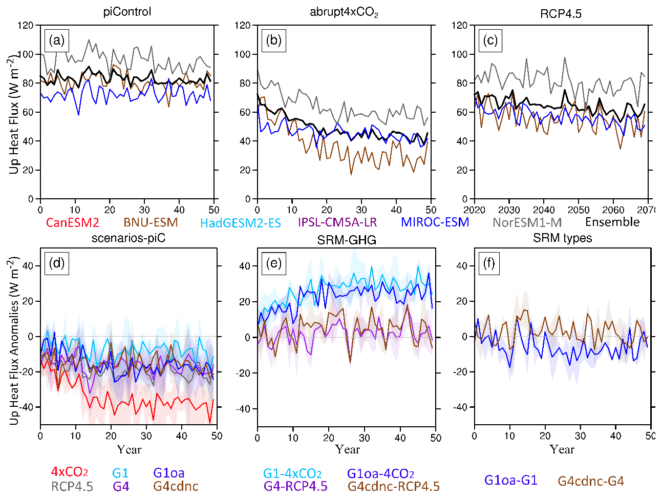
Figure 7The 11-year running annual means simulated by the six ESMs and their ensemble mean of the upward heat flux (W m−2) over the 40-year analysis period in the three deep convective regions outlined in Fig. 10 under (a) piControl, (b) abrupt4×CO2 and (c) RCP4.5. Panels (d)–(f) show AMOC anomalies, and panels (g)–(i) show the changes relative to the other scenarios: left column (d, g) relative to piControl; middle (e, h) relative to global warming scenarios; right (f, i) relative to other geoengineering scenarios. Colored bands in panels (d)–(i) represent the across-ESM spread. G1oa refers to G1oceanAlbedo, and piC refers to piControl.

Figure 8Model mean of upward heat flux (W m−2) over the 40-year analysis period in the three deep convective regions outlined in Fig. 6. Only heat flux data from BNU-ESM, MIROC-ESM and NorESM1-M are available. All three ESMs show a high correlation between upward heat flux (area average of the deep convective regions) and AMOC intensity. The solid line is the linear regression trend line of AMOC intensity and upward heat flux (area average of the deep convective regions) over the 40-year analysis period.
Under G1 and G1oceanAlbdedo, the upward heat flux is increased in the deep convective regions relative to abrupt4×CO2, but it is not as high as under the piControl scenario. The changes of upward heat flux in the deep convective region are consistent with those changes in AMOC intensity. AMOC intensity shows a significant correlation with upward heat flux in the three deep convective regions (Fig. 8), although only three models have data fields available. These results show that the change in upward heat flux caused by the modified ocean–atmosphere temperature difference is an important contributor in all ESMs to the change in AMOC intensity in the geoengineering scenarios.
4.3 Freshwater flux (precipitation − evaporation)
In the output data from ESM, the total freshwater flux into the North Atlantic includes precipitation, evaporation, runoff from river and freshwater flux caused by sea ice thermal dynamic change. Due to the lack of data of runoff and freshwater fluxes caused by sea ice and melting of the Greenland ice sheet, we separately analyze the impact of freshwater flux change caused by precipitation minus evaporation (P−E) on AMOC (Shu et al., 2017).
Relative to piControl, P−E increases by 134 and 51 mm yr−1 under abrupt4×CO2 and RCP4.5 scenarios, respectively. P−E under the four geoengineering scenarios we studied are decreased compared to their reference GHG forcing scenarios. Geoengineering methods mitigate the increase in P−E under GHG forcing. AMOC intensity has no significant correlation with freshwater flux in the three deep convective regions (Fig. 9), so P−E is not the main driver of AMOC change under the four geoengineering scenarios we studied.
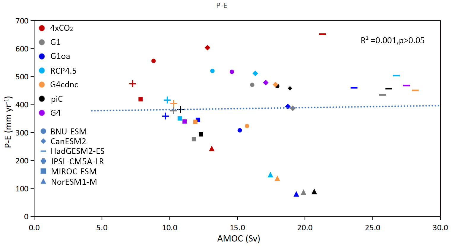
Figure 9Model mean of P−E (mm yr−1) over the 40-year analysis period in the three deep convective regions (outlined in Fig. 6). The dotted line is the linear regression trend line of AMOC intensity and upward heat flux (area average of the deep convective regions) over the 40-year analysis period in all six ESMs.
4.4 September sea ice extent
Arctic surface temperatures have risen 2–3 times faster than the global average level, leading to loss of Arctic sea ice (Dai et el., 2019). Stronger seasonal sea ice melting weakens the AMOC intensity by injecting freshwater and increasing its storage in the North Atlantic (Li and Fedorov, 2021). But sea ice cover also reduces heat transport from the sea to the air and hence inhibits ocean convection, which may weaken AMOC (Drijfhout et al., 2012). Therefore, we can analyze the relationship between AMOC intensity and the freshwater flux changes caused by Arctic sea ice thermodynamics via Arctic sea ice extent changes under the four geoengineering scenarios.
There is almost no September sea ice in the northern North Atlantic in any scenario (Fig. 10). The sea ice extent changes most in the northern seas along the Eurasian Arctic coast. Under both abrupt4×CO2 and RCP4.5 scenarios, Arctic sea ice area is greatly reduced (Fig. 10b, c).
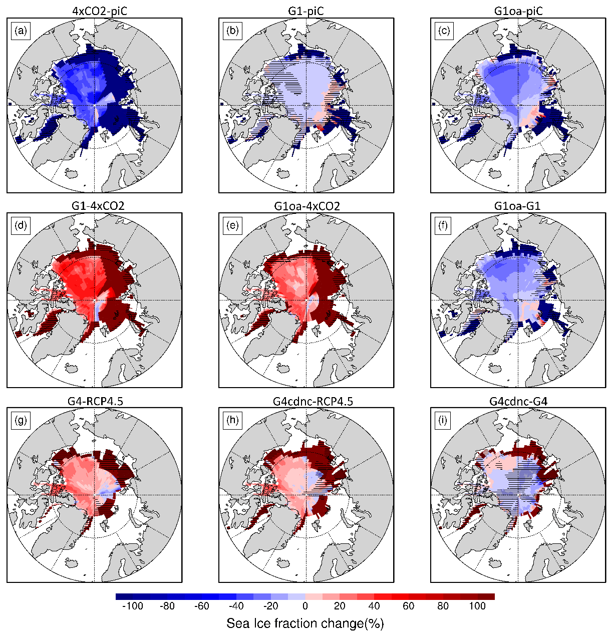
Figure 10Six ESMs and ensemble mean Arctic minimum sea ice fraction percentage changes (defined as the limit of the 15 % ice concentration region) in September in different scenarios (11–50 years). Stippling indicates regions where differences are not significant at the 95 % level according to the Wilcoxon signed-rank test.
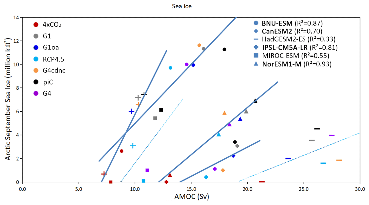
Figure 11Model mean Arctic September sea ice area (106 km2) over the 40-year analysis period (defined as the limit of 15 % ice concentration region). The lines are the linear regression trend lines of AMOC intensity and Arctic September Sea ice area over the 40-year analysis period for each ESM. Those significant at the 95 % level are shown as heavier lines, and the ESMs are labeled in bold in the legend.
Under the G1 scenario, the spatial pattern of September sea ice is changed relative to piControl, with extent changes of up to 20 % regionally and in total reduced by 3 % in an eight-model ensemble (Moore et al., 2014). In our study, relative to piControl, the ensemble mean of six ESMs sea ice area is decreased by about 9 % under G1 and 25 % under G1oceanAlbedo, which is consistent with their AMOC changes. Indeed, the sea ice of the Norwegian Sea is slightly increased under G1 and G1oceanAlbedo relative to piControl (Fig. 10b, c). Compared to abrupt4×CO2, September sea ice increases significantly under G1 by about 80 % and by about 64 % by G1oceanAlbedo. G1oceanAlbedo produces about 16 % less sea ice area than G1 (Table 3). This shows that G1oceanAlbedo and G1 can mitigate the reduction of Arctic September sea ice caused by GHG forcing, and the mitigation effect under G1 is stronger than G1oceanAlbedo.
Under G4 and G4cdnc, the September sea ice significantly increased by about 22 % and 28 % compared to RCP4.5. G4cdnc generally increases sea ice area by 6 % more than G4 (Table 3), consistent with AMOC behavior under the two scenarios. All six ESMs agree that the mitigation on the reduction of Arctic September sea ice area under solar dimming is stronger than with MCB and SAI. Mitigation of sea ice loss under G1oceanAlbedo is stronger than G4cdnc, which is all consistent with AMOC behavior under the four scenarios.
To examine the dependence of sea ice extent on AMOC, we plot the 40-year mean values for all models and all scenarios (Fig. 11). Such plots can determine how linear relations are, as well as their across-model differences. In four of the ESMs, AMOC is significantly correlated (p<0.05) with Arctic sea ice area, HadGem2-ES and MIROC-ESM being the ESM without a significant relationship. Although most ESMs do have significant relationships between minimum sea ice extent and AMOC strength, the models themselves show large differences in strength of the response, in part due to their AMOC strength in the control simulations but also in the changes in September ice extent across the scenarios as seen by the slope of the regression lines in Fig. 11.
There is no significant correlation between AMOC and P−E but significant correlation between AMOC and Arctic September sea ice area. This also shows that the freshwater changes caused by Arctic September sea ice is a key factor in AMOC changes under the four geoengineering experiments. The slopes of the regression lines in Fig. 11 are positive, meaning that greater AMOC strength is correlated with greater ice extent. However, Fig. 3e also shows that heat transport anomalies under the geoengineering scenarios change sign at about 60∘ N, with reductions in heat transport in the south coinciding with increases to the north of 60∘ N. But correlations of heat transport across 60∘ N with sea ice extent for separate ESM across scenarios are all insignificant and vary in sign (Fig. S3), in stark contrast to the regression lines in Fig. 11. For individual scenarios, there are significant anticorrelations only for the RCP4.5, G4 and G4cdnc scenarios (Fig. S4). In this respect, the behavior is similar, although less robust, as for wind forcing in Fig. 5, where scenario impacts as expected, but a consistent relation between scenarios simulated by each ESM is not present. The stronger sea ice correlation with increased AMOC suggests that sea ice may be driving changes in AMOC through the change in freshwater budget.
The mitigation of AMOC intensity, northward heat flux and sea ice extent changes caused by global warming under G1 is significantly stronger than under G1oceanAlbedo. The mitigation under G4cdnc is slightly stronger than G4. The radiative fluxes of the abrupt4×CO2 experiments are 7–8 times greater than those under the RCP4.5 scenarios, as are changes induced in mean and extreme temperatures (Ji et al., 2018). The relative change in AMOC under G4 compared to G1 relative to appropriate controls is similar at about 15 %. This compares with about 25 % effectivity for G4cdnc relative to G1 and 33 % relative to G1oceanAlbedo (Table S3). Heat content effectivity for G4 relative to G1 is around 25 %, and for G4cdnc the ensemble effectiveness is over 40 % of G1oceanAlbedo (Table S3). The changes in September sea ice extent effectiveness under G4 are about 30 % of those under G1 and 50 % for G4cdnc relative to G1oceanAlbedo. This might mean that specific measures under G4cdnc appear more effective than those simulated under G4 stratospheric aerosol injection, but the forcing applied under G4cdnc was not specifically designed to match the net radiative forcing of the G4 SAI.
We want to examine the differences in response to type of SRM as defined in the GeoMIP experiments we analyze. The ESMs have different sensitivities to climate forcing, so we normalize the model fields with top-of-atmosphere radiative forcing (TOA), e.g.,
which represents AMOC changes per unit change of the corresponding TOA radiation flux changes.
Because of the large differences in forcing magnitude between, for example, Abrupt4×CO2 and RCP4.5, we cannot simply look at anomalies, but instead we can compare the responses as a ratio; for example,
compares the SAI and the solar dimming anomalies.
Then we compare the efficacy of different mitigation experiments by the ratio of their sensitivity parameters; for example, the measure of efficacy in the example of comparing the SAI and the solar dimming anomalies above becomes
which we can calculate for upward heat flux and September sea ice extent in addition to AMOC, as well as for ratios indicative of the relative responses of MCB to solar dimming and SAI to MCB. The ensemble means indicate the typical differences in efficacy between type of geoengineering (Table 4).
Table 4Across-ESM ensemble mean relative efficacy ratios of geoengineering compared to their efficacy in changing TOA radiation. Where individual ESM have no data, the ensemble mean was used.
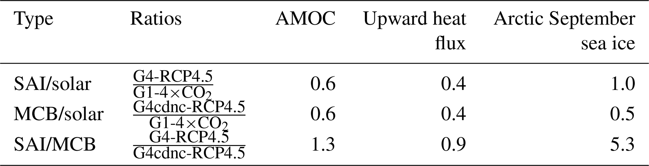
Table 4 shows that changes to AMOC and upward heat flux are less than for overall climate sensitivity measured as TOA since the ratios are all less than 1. The relative efficacy by SAI and MCB for AMOC and upward heat fluxes are about half those of solar dimming. Comparing MCB and SAI shows smaller differences, with relative efficacies closer to unity. Arctic September sea ice extent indicates larger differences between type of geoengineering, with SAI being more effective than MCB in the experiments analyzed here. Different ESMs have different responses to MCB and SAI, especially in the comparison between G4cdnc and G4. Individual model results are shown in Tables S6–S8.
Five out of six ESMs agree that SAI is more effective than MCB for AMOC (Table S6), with the outlier being HadGEM2-ES. This model is also the only one with greater AMOC intensity under the RCP4.5 and G4 scenarios than in piControl. HadGEM2-ES is also unique in displaying no correlation between wind speed and AMOC (Fig. 5), and along with MIROC-ESM it shows an insignificant relation between AMOC and September sea ice extent (Fig. 11).
There is lower consensus on which of SAI or MCB is more effective, with the ESM split three against three. In the case of upward heat flux (Table S7), the ESMs generally agree that solar dimming is more effective than either SAI or MCB with little to choose between SAI and MCB. For September sea ice (Table S8), SAI clearly outscores MCB in all but one (BNU-ESM) of the models and experiments we analyzed, while SAI and solar dimming are fairly similar in effectiveness across the ESMs.
The proximate factor from our analysis of the main drivers of changes under the different scenarios is the change in heat flux transported from ocean to atmosphere caused by the air–sea temperature difference changes in deep convective regions of the North Atlantic (Fig. 7). This is consistent with the analysis of the G1 experiment (Hong et al., 2017). All the geoengineering scenarios produce surface cooling, which partially restores the ocean–atmosphere temperature contrast altered by GHG forcing and thus increases the heat flux from ocean to atmosphere. In the three deep convection regions of the northern North Atlantic (Fig. 6), the ocean temperature is usually higher than the near-surface temperature, and the surface seawater originating from the tropics can release heat to the atmosphere and cool down. Global warming increases the near-surface air temperature, reducing the air–sea heat exchange. While geoengineering might be expected to ameliorate this problem by cooling the atmosphere, we found that the surface air temperatures in the deep convection regions of the North Atlantic remained higher than in piControl, even in scenarios in which the global radiative budget is balanced. Thus, the geoengineering scenarios had an intermediate amount of AMOC weakening, in between the preindustrial state and unmitigated global warming. The decrease of surface seawater density in the northern North Atlantic caused by the increase in surface seawater temperature weakens the surface seawater subsidence in this area under the four SRM geoengineering scenarios as compared to piControl.
While changes in upward heat flux over the three convective regions play a prominent role, the freshwater flux changes caused by Arctic sea ice melting may also affect AMOC changes under geoengineering. Sea ice melting releases large amounts of freshwater into the North Atlantic. In the deep convection regions of the North Atlantic, the injection of a large amount of freshwater reduces the density of surface seawater, hindering surface water sinking and weakening AMOC. Although the wintertime formation of Arctic sea ice increases the density of the surface water in the Arctic, promoting surface water sinking in the deep convection regions of the North Atlantic, the sustained decline in Arctic sea ice and strengthened seasonal cycle produces a gradual freshening of the upper Arctic Ocean (Li and Federov, 2021). Wang et al. (2019) note that sea ice decline is likely to have a remarkable influence on the ocean environment and that sea ice decline impacts on dynamical processes should be considered. Climate model sensitivity studies perturbing both sea ice and radiative forcing (Sévellec et al., 2017; Liu et al., 2018; Liu and Fedorov, 2019) elucidate how buoyancy anomalies may escape the Arctic into ocean deep convection regions, weakening the AMOC. The four geoengineering experiments may thus mitigate the AMOC weakening caused by GHG forcing through increasing the September Arctic sea ice area and reducing sea ice seasonality. The changes of Arctic sea ice area and AMOC are interactive, and the changes of Arctic September sea ice area are significantly correlated under different scenarios (except for HadGEM2-ES). However, the response is ESM dependent as the relationship between AMOC changes and Arctic sea ice area changes are different. A key uncertainty when it comes to the AMOC in the future is the melting of the Greenland ice sheet. More realistic modeling of the ice sheet, sensitivity studies (e.g., Swingedouw et al., 2015) or indeed interactive ice sheet modeling would be needed to address this, which is beyond the scope of this study.
Changes in near-surface wind speed are known to alter the speed of northward surface water transport and hence AMOC. The effects of wind speed appear on short timescales (Yang et al., 2016). Near-surface wind speed changes over North Atlantic are correlated with AMOC under many of the different scenarios, but they are not significantly correlated across scenarios simulated by each ESM. Thus, scenario impacts wind speed as expected, but a consistent relation between scenarios simulated by each ESM is not evident. Hence, near-surface wind speed is not the main factor of AMOC changes under different scenarios.
GHG forcing weakens AMOC intensity, reducing northward ocean heat transport. The three SRM methods we studied, solar dimming (G1), MCB (G1oceanAlbedo and G4cdnc) and SAI (G4) mitigate the AMOC weakening caused by GHG forcing. The mitigation effects of AMOC weakening under MCB are similar to SAI, but both are relatively less effective than solar dimming in these experiments. All four geoengineering scenarios demonstrate weakened AMOC compared to the piControl scenario. The drivers producing the changes in AMOC are dominated by the differences in surface air–ocean temperatures, with the radiative cooling produced by the SRM tending to reverse the GHG changes. We found no relationship between freshwater flux due to river flow or imbalance in precipitation − evaporation and changes in AMOC, but there is a significant correlation between September sea ice extent and AMOC intensity. The bigger the decline in sea ice extent, the stronger the reduction in AMOC intensity. The strong statistical relationship for most models across scenarios suggests that AMOC is not directly driving sea ice reduction since a lower AMOC means less ocean heat transport. Instead, it supports modeling studies that indicate freshening mechanisms in the deep convection regions associated with greater sea ice seasonality that may act to reduce AMOC as summer sea ice is removed.
All data used in this study, except for parts of the data of NorESM1-M and IPSL-CM5A-LR, are available from the Coupled Model Intercomparison Project 5 (CMIP5) network https://esgf-node.llnl.gov/search/cmip5/, established by the World Climate Research Programme (WCRP) the Working Group on Coupled Modelling (WGCM), 2022). The NorESM1-M and IPSL-CM5A-LR data are archived by the modeling team.
The supplement related to this article is available online at: https://doi.org/10.5194/acp-22-4581-2022-supplement.
JCM and MX conceived and designed the analysis. MX mainly collected all the data and performed the analysis. MX wrote the paper, and JCM, LZ, MW and HM provided critical suggestions and revised the paper. All authors contributed to the discussion.
The contact author has declared that neither they nor their co-authors have any competing interests.
Publisher's note: Copernicus Publications remains neutral with regard to jurisdictional claims in published maps and institutional affiliations.
This article is part of the special issue “Resolving uncertainties in solar geoengineering through multi-model and large-ensemble simulations (ACP/ESD inter-journal SI)”. It is not associated with a conference.
This study is supported by the National Key Research and Development Program of China (grant nos. 2021YFB3900105, 2018YFC1406104), the National Natural Science Foundation of China (grant no. 41941006), and Finnish Academy COLD Consortium (grant no. 322430). We thank two anonymous reviewers that made many suggestions to help improve the paper.
This research has been supported by the National Key Research and Development Program of China (grant nos. 2021YFB3900105, 2018YFC1406104), the National Natural Science Foundation of China (grant no. 41941006), and Finnish Academy COLD Consortium (grant no. 322430).
This paper was edited by Hailong Wang and reviewed by two anonymous referees.
Ahlm, L., Jones, A., Stjern, C. W., Muri, H., Kravitz, B., and Kristjánsson, J. E.: Marine cloud brightening – as effective without clouds, Atmos. Chem. Phys., 17, 13071–13087, https://doi.org/10.5194/acp-17-13071-2017, 2017.
Angel, R.: Feasibility of cooling the Earth with a cloud of small spacecraft near the inner Lagrange point (L1), P. Natl. Acad. Sci. USA., 103, 17184–17189, 2006.
Bentsen, M., Bethke, I., Debernard, J. B., Iversen, T., Kirkevåg, A., Seland, Ø., Drange, H., Roelandt, C., Seierstad, I. A., Hoose, C., and Kristjánsson, J. E.: The Norwegian Earth System Model, NorESM1-M – Part 1: Description and basic evaluation of the physical climate, Geosci. Model Dev., 6, 687–720, https://doi.org/10.5194/gmd-6-687-2013, 2013.
Buckley, M. W. and Marshall, J.: Observations, inferences, and mechanisms of the Atlantic Meridional Overturning Circulation: A review, Rev. Geophys., 54, 5–63, https://doi.org/10.1002/2015RG000493, 2016.
Cao, L., Duan, L., Bala, G., and Caldeira, K.: Simultaneous stabilization of global temperature and precipitation through cocktail geoengineering, Geophys. Res. Lett., 44, 7429–7437, https://doi.org/10.1002/2017GL074281, 2017.
Chen, X. and Tung, K. K.: Global surface warming enhanced by weak Atlantic overturning circulation, Nature, 559, 387–391, https://doi.org/10.1038/s41586-018-0320-y, 2018.
Cheng, W., Chiang, J. C. H., and Zhang, D.: Atlantic Meridional Overturning Circulation (AMOC) in CMIP5 Models: RCP and Historical Simulations, J. Climate, 26, 7187–7197, https://doi.org/10.1175/JCLI-D-12-00496.1, 2013.
Collins, W. J., Bellouin, N., Doutriaux-Boucher, M., Gedney, N., Halloran, P., Hinton, T., Hughes, J., Jones, C. D., Joshi, M., Liddicoat, S., Martin, G., O'Connor, F., Rae, J., Senior, C., Sitch, S., Totterdell, I., Wiltshire, A., and Woodward, S.: Development and evaluation of an Earth-System model – HadGEM2, Geosci. Model Dev., 4, 1051–1075, https://doi.org/10.5194/gmd-4-1051-2011, 2011.
Dai, A., Luo, D., Song, M., and Liu, J.: Arctic amplification is caused by sea-ice loss under increasing CO2, Nature Commun., 10, 1–13, https://doi.org/10.1038/s41467-018-07954-9, 2019.
Drijfhout, S., Oldenborgh, G. T., and Cimatoribus, A.: Is a Decline of AMOC Causing the Warming Hole above the North Atlantic in Observed and Modeled Warming Patterns?, J. Climate, 25, 8373–8379, https://doi.org/10.1175/JCLI-D-12-00490.1, 2012.
Dufresne, J.-L., Foujols, M.-A., Denvil, S., Caubel, A., Marti, O., Aumont, O., Balkanski, Y., Bekki, S., Bellenger, H., Benshila, R., Bony, S., Bopp, L., Braconnot, P., Brockmann, P., Cadule, P., Cheruy, F., Codron, F., Cozic, A., Cugnet, D., de Noblet, N., Duvel, J.-P., Ethe, C., Fairhead, L., Fichefet, T., Flavoni, S., Friedlingstein, P., Grandpeix, J.-Y., Guez, L., Guilyardi, E., Hauglustaine, D., Hourdin, F., Idelkadi, A., Ghattas, J., Joussaume, S., Kageyama, M., Krinner, G., Labetoulle, S., Lahellec, A., Lefebvre, M.-P., Lefevre, F., Levy, C., Li, Z. X., Lloyd, J., Lott, F., Madec, G., Mancip, M., Marchand, M., Masson, S., Meurdesoif, Y., Mignot, J., Musat, I., Parouty, S., Polcher, J., Rio, C., Schulz, M., Swingedouw, D., Szopa, S., Talandier, C., Terray, P., Viovy, N., and Vuichard, N.: Climate change projections using the IPSL-CM5 Earth System Model: from CMIP3 to CMIP5, Clim. Dynam., 40, 2123–2165, https://doi.org/10.1007/s00382-012-1636-1, 2013.
Frajka-Williams, E., Ansorge, I. J., Baehr, J., Bryden, H. L., Chidichimo, M. P., Cunningham, S. A., Danabasoglu, G., Dong, S., Donohue, K. A., Elipot, S., Heimbach, P., Holliday, N. P., Hummels, R., Jackson, L. C., Karstensen, J., Lankhorst, M., Le Bras, I. A., Lozier, M. S., McDonagh, E. L., Meinen, C. S., Mercier, H., Moat, B. I., Perez, R. C., Piecuch, C. G., Rhein, M., Srokosz, M. A., Trenberth, K. E., Bacon, S., Forget, G., Goni, G., Kieke, D., Koelling, J., Lamont, T., McCarthy, G. D., Mertens, C., Send, U., Smeed, D. A., Speich, S., van den Berg, M., Volkov, D., and Wilson, C.: Atlantic Meridional Overturning Circulation: Observed Transport and Variability, Front. Mar. Sci., 6, 260, https://doi.org/10.3389/fmars.2019.00260, 2019.
Gent, P. R., Bryan, F. O., Danabasoglu, G., Doney, S. C., Holland, W. R., Large, W. G., and McWilliams, J. C.: The NCAR Climate System Model Global Ocean Component, J. Climate, 11, 1287–1306, https://doi.org/10.1175/1520-0442(1998)011<1287:TNCSMG>2.0.CO;2, 1998.
Griffies, S. M.: Elements of MOM4p1, GFDL Ocean Group Technical Report No. 6, NOAA/Geophysical Fluid Dynamics Laboratory, 444 pp., 2010.
Hong, Y., Moore, J. C., Jevrejeva, S., Ji, D., Phipps, S. J., Lenton, A., Tilmes, S., Watanabe, S., and Zhao, L.: Impact of the GeoMIP G1 sunshade geoengineering experiment on the Atlantic meridional overturning circulation, Environ. Res. Lett., 12, 034009, https://doi.org/10.1088/1748-9326/aa5fb8, 2017.
Iversen, T., Bentsen, M., Bethke, I., Debernard, J. B., Kirkevåg, A., Seland, Ø., Drange, H., Kristjansson, J. E., Medhaug, I., Sand, M., and Seierstad, I. A.: The Norwegian Earth System Model, NorESM1-M – Part 2: Climate response and scenario projections, Geosci. Model Dev., 6, 389–415, https://doi.org/10.5194/gmd-6-389-2013, 2013.
Ji, D., Wang, L., Feng, J., Wu, Q., Cheng, H., Zhang, Q., Yang, J., Dong, W., Dai, Y., Gong, D., Zhang, R.-H., Wang, X., Liu, J., Moore, J. C., Chen, D., and Zhou, M.: Description and basic evaluation of Beijing Normal University Earth System Model (BNU-ESM) version 1, Geosci. Model Dev., 7, 2039–2064, https://doi.org/10.5194/gmd-7-2039-2014, 2014.
Ji, D., Fang, S., Curry, C. L., Kashimura, H., Watanabe, S., Cole, J. N. S., Lenton, A., Muri, H., Kravitz, B., and Moore, J. C.: Extreme temperature and precipitation response to solar dimming and stratospheric aerosol geoengineering, Atmos. Chem. Phys., 18, 10133–10156, https://doi.org/10.5194/acp-18-10133-2018, 2018.
Johns, W. E., Baringer, M. O., Beal, L. M., Cunningham, S. A., Kanzow, T., Bryden, H. L., Hirschi, J. J. M., Marotzke, J., Meinen, C. S., Shaw, B., and Curry, R.: Continuous, Array-Based Estimates of Atlantic Ocean Heat Transport at 26.5∘ N, J. Climate, 24, 2429–2449, https://doi.org/10.1175/2010JCLI3997.1, 2011.
Jones, A., Haywood, J., and Boucher, O.: A comparison of the climate impacts of geoengineering by stratospheric SO2 injection and by brightening of marine stratocumulus cloud, Atmos. Sci. Let., 12, 176–183, https://doi.org/10.1002/asl.291, 2011.
K-1 Model Developers: K-1 Coupled GCM (MIROC) description, K-1 Tech Report No. 1. Center for Climate System Research, University of Tokyo, National Institute for Environmental Studies, Frontier Research Center for Global Change, edited by: edited by Hasumi, H., and Emori, S., https://ccsr.aori.u-tokyo.ac.jp/~hasumi/miroc_description.pdf#:~:text=The%20Model%20for%20Interdisciplinary%20Research%20on%20Climate%20%28MIROC%29%2C,interacts%20with%20the%20land%20and%20sea%20ice%20components (last access: 4 April 2022), 2004.
Keith, D. W.: Geoengineering the climate: History and prospect, Annu. Rev. Energ. Env., 25, 245–284, https://doi.org/10.1146/annurev.energy.25.1.245, 2000.
Kravitz, B., Robock, A., Boucher, O., Schmidt, H., Taylor, K. E., Stenchikov, G., and Schulz, M.: The Geoengineering Model Intercomparison Project (GeoMIP), Atmos. Sci. Let., 12, 162–167, https://doi.org/10.1002/asl.316, 2011.
Kravitz, B., Forster, P. M., Jones, A., Robock, A., Alterskjær, K., Boucher, O., Jenkins, A. K. L., Korhonen, H., Kristjánsson, J. E., Muri, H., Niemeier, U., Partanen, A. I., Rasch, P. J., Wang, H., and Watanabe, S.: Sea spray geoengineering experiments in the geoengineering model intercomparison project (GeoMIP): Experimental design and preliminary results, J. Geophys. Res.-Atmos., 118, 11175–11186, https://doi.org/10.1002/jgrd.50856, 2013.
Kravitz, B., Robock, A., Tilmes, S., Boucher, O., English, J. M., Irvine, P. J., Jones, A., Lawrence, M. G., MacCracken, M., Muri, H., Moore, J. C., Niemeier, U., Phipps, S. J., Sillmann, J., Storelvmo, T., Wang, H., and Watanabe, S.: The Geoengineering Model Intercomparison Project Phase 6 (GeoMIP6): simulation design and preliminary results, Geosci. Model Dev., 8, 3379–3392, https://doi.org/10.5194/gmd-8-3379-2015, 2015.
Kravitz, B., MacMartin, D. G., Wang, H., and Rasch, P. J.: Geoengineering as a design problem, Earth Syst. Dynam., 7, 469–497, https://doi.org/10.5194/esd-7-469-2016, 2016.
Kravitz, B., Rasch, P. J., Wang, H., Robock, A., Gabriel, C., Boucher, O., Cole, J. N. S., Haywood, J., Ji, D., Jones, A., Lenton, A., Moore, J. C., Muri, H., Niemeier, U., Phipps, S., Schmidt, H., Watanabe, S., Yang, S., and Yoon, J.-H.: The climate effects of increasing ocean albedo: an idealized representation of solar geoengineering, Atmos. Chem. Phys., 18, 13097–13113, https://doi.org/10.5194/acp-18-13097-2018, 2018.
Latham, J., Bower, K., Choularton, T., Coe, H., Connolly, P., Cooper, G., Craft, T., Foster, J., Gadian, A., Galbraith, L., Iacovides, H., Johnston, D., Launder, B., Leslie, B., Meyer, J., Neukermans, A., Ormond, B., Parkes, B., Rasch, P., Rush, J., Salter, S., Stevenson, T., Wang, H., Wang, Q., and Wood, R.: Marine cloud brightening, Philos. T. R. Soc. A., 370, 4217–4262, https://doi.org/10.1098/rsta.2012.0086, 2012.
Li, H. and Fedorov, A. V.: Persistent freshening of the Arctic Ocean and changes in the North Atlantic salinity caused by Arctic sea ice decline, Clim. Dynam., 57, 2995–3013, https://doi.org/10.1007/s00382-021-05850-5, 2021.
Liu, W. and Fedorov, A. V.: Global impacts of Arctic sea ice loss mediated by the atlantic meridional overturning circulation, Geophys. Res. Lett., 46, 944–952, https://doi.org/10.1029/2018GL080602, 2019.
Liu, W., Fedorov, A., and Sevellec, F.: The mechanisms of the Atlantic Meridional Overturning Circulation slowdown induced by Arctic sea ice decline, J. Climate, 32, 977–996, https://doi.org/10.1175/JCLI-D-18-0231.1, 2018.
Malik, A., Nowack, P. J., Haigh, J. D., Cao, L., Atique, L., and Plancherel, Y.: Tropical Pacific climate variability under solar geoengineering: impacts on ENSO extremes, Atmos. Chem. Phys., 20, 15461–15485, https://doi.org/10.5194/acp-20-15461-2020, 2020.
McCarthy, G. D., Brown, P. J., Flagg, C. N., Goni, G., Houpert, L., Hughes, C. W., Hummels, R., Inall, M., Jochumsen, K., Larsen, K. M. H., Lherminier, P., Meinen, C. S., Moat, B. I., Rayner, D., Rhein, M., Roessler, A., Schmid, C., and Smeed, D. A.: Sustainable Observations of the AMOC: Methodology and Technology, Rev. Geophys., 58, e2019RG000654, https://doi.org/10.1029/2019RG000654, 2019.
Moore, J. C., Rinke, A., Yu, X., Ji, D., Cui, X., Li, Y., Alterskjær, K., Kristjánsson, J. E., Muri, H., Boucher, O., Huneeus, N., Kravitz, B., Robock, A., Niemeier, U., Schulz, M., Tilmes, S., Watanabe, S., Yang, S.: Arctic sea ice and atmospheric circulation under the GeoMIP G1 scenario, J. Geophys. Res.-Atmos., 119, 567–583, https://doi.org/10.1002/2013JD021060, 2014.
Moore, J. C., Yue, C., Zhao, L., Guo, X., Watanabe, S., and Ji, D.: Greenland Ice Sheet Response to Stratospheric Aerosol Injection Geoengineering, Earth's Future., 7, 1451–1463, https://doi.org/10.1029/2019EF001393, 2019.
Muri, H., Tjiputra, J., Otterå, O. H., Adakudlu, M., Lauvset, S. K., Grini, A., Schulz, M., Niemeier, U., and Kristjánsson, J. E.: Climate response to aerosol geoengineering: A multimethod comparison, J. Climate, 31, 6319–6340, https://doi.org/10.1175/JCLI-D-17-0620.1, 2018.
Niemeier, U., Schmidt, H., Alterskjær, K., and Kristjánsson, J. E.: Solar irradiance reduction via climate engineering: Impact of different techniques on the energy balance and the hydrological cycle, J. Geophys. Res.-Atmos., 118, 11905–11917, https://doi.org/10.1002/2013JD020445, 2013.
Roberts, C. D., Jackson, L., and McNeall, D.: Is the 2004–2012 reduction of the Atlantic meridional overturning circulation significant?, Geophys. Res. Lett., 41, 3204–3210, https://doi.org/10.1002/2014GL059473, 2014.
Send, U., Lankhorst, M., and Kanzow, T.: Observation of decadal change in the Atlantic meridional overturning circulation using 10 years of continuous transport data, Geophys. Res. Lett., 38, L24606, https://doi.org/10.1029/2011GL049801, 2011.
Sévellec, F., Fedorov, A. V., and Liu, W.: Arctic sea-ice decline weakens the Atlantic Meridional Overturning Circulation, Nat. Clim. Change, 7, 604–610, https://doi.org/10.1038/nclimate3353, 2017.
Shu, Q., Qiao, F., Song, Z., and Xiao, B.: Effect of increasing Arctic river runoff on the Atlantic meridional overturning circulation: a model study, Acta Oceanol. Sin., 36, 1–7, https://doi.org/10.1007/s13131-017-1009-z, 2017.
Smeed, D. A., Josey, S. A., Beaulieu, C., Johns, W. E., Moat, B. I., Frajka-Williams, E., Rayner, D., Meinen, C. S., Baringer, M. O., Bryden, H. L., and McCarthy, G. D.: The North Atlantic Ocean Is in a State of Reduced Overturning, Geophys. Res. Lett., 45, 1527–1533, https://doi.org/10.1002/2017GL076350, 2018.
Smith, W. and Wagner, G.: Stratospheric aerosol injection tactics and costs in the first 15 years of deployment, Environ. Res. Lett., 13, 124001, https://doi.org/10.1088/1748-9326/aae98d, 2018.
Smyth, J. E., Russotto, R. D., and Storelvmo, T.: Thermodynamic and dynamic responses of the hydrological cycle to solar dimming, Atmos. Chem. Phys., 17, 6439–6453, https://doi.org/10.5194/acp-17-6439-2017, 2017.
Stouffer, R. J., Eyring, V., Meehl, G. A., Bony, S., Senior, C., Stevens, B., and Taylor, K. E.: CMIP5 scientific gaps and recommendations for CMIP6, B. Am. Meteorol. Soc., 98, 95–105, https://doi.org/10.1175/BAMS-D-15-00013.1, 2017.
Swingedouw, D., Rodehacke, C. B., Olsen, S. M., Menary, M., Gao, Y., Mikolajewicz, U., and Mignot, J.: On the reduced sensitivity of the Atlantic overturning to Greenland ice sheet melting in projections: a multi-model assessment, Clim. Dynam., 44, 3261–3279, https://doi.org/10.1007/s00382-014-2270-x, 2015.
Taylor, K. E., Stouffer, R. J., and Meehl, G. A.: An overview of CMIP5 and the experiment design, B. Am. Meteorol. Soc., 93, 485–498, https://doi.org/10.1175/BAMS-D-11-00094.1, 2012.
Thornalley, D. J. R., Oppo, D. W., Ortega, P., Robson, J. I., Brierley, C. M., Davis, R., Hall, I. R., Moffa-Sanchez, P., Rose, N. L., Spooner, P. T., Yashayaev, I., and Keigwin, L. D.: Anomalously weak Labrador Sea convection and Atlantic overturning during the past 150 years, Nature, 556, 227–230, https://doi.org/10.1038/s41586-018-0007-4, 2018.
Tilmes, S., MacMartin, D. G., Lenaerts, J. T. M., van Kampenhout, L., Muntjewerf, L., Xia, L., Harrison, C. S., Krumhardt, K. M., Mills, M. J., Kravitz, B., and Robock, A.: Reaching 1.5 and 2.0 °C global surface temperature targets using stratospheric aerosol geoengineering, Earth Syst. Dynam., 11, 579–601, https://doi.org/10.5194/esd-11-579-2020, 2020.
Watanabe, S., Hajima, T., Sudo, K., Nagashima, T., Takemura, T., Okajima, H., Nozawa, T., Kawase, H., Abe, M., Yokohata, T., Ise, T., Sato, H., Kato, E., Takata, K., Emori, S., and Kawamiya, M.: MIROC-ESM 2010: model description and basic results of CMIP5-20c3m experiments, Geosci. Model Dev., 4, 845–872, https://doi.org/10.5194/gmd-4-845-2011, 2011.
Wang, Q., Wekerle, C., Danilov, S., Sidorenko, D., Koldunov, N., Sein, D., Rabe, B., and Jung, T.: Recent Sea Ice Decline Did Not Significantly Increase the Total Liquid Freshwater Content of the Arctic Ocean, J. Climate, 32, 15–32, 2019.
Weijer, W., Cheng, W., Garuba, O. A., Hu, A., and Nadiga, B. T.: CMIP6 Models Predict Significant 21st Century Decline of the Atlantic Meridional Overturning Circulation, Geophys. Res. Lett., 47, e2019GL086075, https://doi.org/10.1029/2019GL086075, 2020.
World Climate Research Programme (WCRP) the Working Group on Coupled Modelling (WGCM): Coupled Model Intercomparison Project 5 (CMIP5) network, https://esgf-node.llnl.gov/search/cmip5/, last access: 4 April 2022.
Yang, D. and Saenko, O. A.: Ocean heat transport and its projected change in CanESM2, J. Climate, 25, 8148–8163, https://doi.org/10.1175/JCLI-D-11-00715.1, 2012.
Yang, H., Wang, K., Dai, H., Wang, Y., and Li, Q.: Wind effect on the Atlantic meridional overturning circulation via sea ice and vertical diffusion, Clim. Dynam., 46, 3387–3403, https://doi.org/10.1007/s00382-015-2774-z, 2016.
Zhao, J. and Johns, W.: Wind-forced interannual variability of the Atlantic meridional overturning circulation at 26.5∘ N, J. Geophys. Res.-Oceans, 119, 2403–2419, https://doi.org/10.1002/2013JC009407, 2014.