Atmospheric rivers and associated precipitation patterns during the ACLOUD and PASCAL campaigns near Svalbard (May–June 2017): case studies using observations, reanalyses, and a regional climate model

Recently, a significant increase in the atmospheric moisture content has been documented over the Arctic, where both local contributions and poleward moisture transport from lower latitudes can play a role. This study focuses on the anomalous moisture transport events confined to long and narrow corridors, known as atmospheric rivers (ARs), which are expected to have a strong influence on Arctic moisture amounts, precipitation, and the energy budget. During two concerted intensive measurement campaigns – Arctic CLoud Observations Using airborne measurements during polar Day (ACLOUD) and the Physical feedbacks of Arctic planetary boundary layer, Sea ice, Cloud and AerosoL (PASCAL) – that took place at and near Svalbard, three high-water-vapour-transport events were identified as ARs, based on two tracking algorithms: the 30 May event, the 6 June event, and the 9 June 2017 event. We explore the temporal and spatial evolution of the events identified as ARs and the associated precipitation patterns in detail using measurements from the French (Polar Institute Paul Emile Victor) and German (Alfred Wegener Institute for Polar and Marine Research) Arctic Research Base (AWIPEV) in Ny-Ålesund, satellite-borne measurements, several reanalysis products (the European Centre for Medium-Range Weather Forecasts (ECMWF) Re-Analysis (ERA) Interim (ERA-Interim); the ERA5 reanalysis; the Modern-Era Retrospective analysis for Research and Applications, version 2 (MERRA-2); the Climate Forecast System version 2 (CFSv2); and the Japanese 55-Year Reanalysis (JRA-55)), and the HIRHAM regional climate model version 5 (HIRHAM5). Results show that the tracking algorithms detected the events differently, which is partly due to differences in the spatial and temporal resolution as well as differences in the criteria used in the tracking algorithms. The first event extended from western Siberia to Svalbard, caused mixed-phase precipitation, and was associated with a retreat of the sea-ice edge. The second event, 1 week later, had a similar trajectory, and most precipitation occurred as rain, although mixed-phase precipitation or only snowfall occurred in some areas, mainly over the coast of north-eastern Greenland and the north-east of Iceland, and no differences were noted in the sea-ice edge. The third event showed a different pathway extending from the north-eastern Atlantic towards Greenland before turning south-eastward and reaching Svalbard. This last AR caused high precipitation amounts on the east coast of Greenland in the form of rain and snow and showed no precipitation in the Svalbard region. The vertical profiles of specific humidity show layers of enhanced moisture that were concurrent with dry layers during the first two events and that were not captured by all of the reanalysis datasets, whereas the HIRHAM5 model misrepresented humidity at all vertical levels. There was an increase in wind speed with height during the first and last events, whereas there were no major changes in the wind speed during the second event. The accuracy of the representation of wind speed by the reanalyses and the model depended on the event. The objective of this paper was to build knowledge from detailed AR case studies, with the purpose of performing long-term analysis. Thus, we adapted a regional AR detection algorithm to the Arctic and analysed how well it identified ARs, we used different datasets (observational, reanalyses, and model) and identified the most suitable dataset, and we analysed the evolution of the ARs and their impacts in terms of precipitation. This study shows the importance of the Atlantic and Siberian pathways of ARs during spring and beginning of summer in the Arctic; the significance of the AR-associated strong heat increase, moisture increase, and precipitation phase transition; and the requirement for high-spatio-temporal-resolution datasets when studying these intense short-duration events.

1 Introduction

The Arctic is a region of major interest due to its high sensitivity to global warming with significant implications for both the regional climate and the global climate system (McGuire et al., 2006). Thus, changes in the Arctic might have implications beyond the region, influencing the mid-latitude climate and weather. For instance, changes during the summer, including a weakening of the storm tracks, a meridional shift in jet position, and an amplification of quasi-stationary waves, can increase the persistence of summer hot and dry extremes at mid-latitudes (Coumou et al., 2018). On the contrary, some studies point to an increase in the probability of the occurrence of severe weather during winter in the mid-latitudes (e.g. central Eurasia – Mori et al., 2019; the eastern US – Cohen et al., 2018), due to the Arctic warming.

A significant increase in the atmospheric moisture content has been documented over the Arctic in the recent years (Rinke et al., 2019; Screen and Simmonds, 2010). This is partially explained by the reduction in sea-ice cover, which enhances local evaporation (Bintanja and Selten, 2014). However, others argue that the predominant reason is the enhanced poleward moisture flux during recent decades (Zhang et al., 2013), which is expected to continuously increase in the future (Bengtsson et al., 2011; Bintanja and Selten, 2014; Kattsov et al., 2007; Skific and Francis, 2013). This might be due to several factors or a combination of them, such as changes in the atmospheric circulation patterns, increased moisture transport intensity, and/or higher evaporation rates in the lower-latitude moisture source regions (Gimeno et al., 2015). However, in their review, Gimeno et al. (2019) reason that there is no agreement in the calculated trends in atmospheric moisture transport to the Arctic.

Extreme poleward moisture transport events towards the Arctic are known as moisture intrusions. Woods et al. (2013) identified an average of 14 moisture intrusions per season, for boreal winters from 1990 to 2010, with a typical duration of 2 to 4 d, corresponding to 28 % of the total poleward moisture transport across 70^∘ N. These moisture intrusions have a filamentary structure, showing similar features to a phenomena known as atmospheric rivers (ARs) (Baggett et al., 2016).

Our study focuses on the ARs, which are recognized by anomalous moisture transport confined to long, narrow, transient corridors. ARs are characterized by a filament of high specific humidity, which is fuelled by the transport of moisture from (sub-)tropical to higher latitudes and/or the moisture convergence along the pre-cold frontal low-level jet of an extratropical cyclone, which is part of the warm conveyor belt (WCB) (Ralph et al., 2004). Extratropical cyclones are low-pressure systems associated with cold, warm, and occluded surface fronts. The water vapour arising from the warm sector of the cyclone converges along the cold front, characterized by cool and dry air, which catches up with the warm front. As a result, a narrow band of high water vapour content is formed ahead of the cold front at the base of the WCB, associated with strong low-level winds.

Multiple studies have analysed the increase in poleward moisture transport into the Arctic region and the associated impacts, including warming (Johansson et al., 2017), decrease in the sea-ice concentration (Lee et al., 2017; Park et al., 2015; Yang and Magnusdottir, 2017), increase in precipitation (Bintanja et al., 2020; Gimeno-Sotelo et al., 2018), and changes in the cloudiness and cloud radiative heating (Johansson et al., 2017). Although ARs have mostly been studied for the western coast of North America and Europe, they have a remarkable importance for the high latitudes. Previous studies have shown that ARs have a strong influence on both Arctic and Antarctic mass and the energy budget of ice sheets (Gorodetskaya et al., 2014, 2020; Mattingly et al., 2018; Nash et al., 2018; Neff et al., 2014; Wille et al., 2019; Woods et al., 2013; Woods and Caballero, 2016).

In the Arctic latitudes, the enhanced poleward moisture transport is related to an increase in precipitation (Bintanja et al., 2020; Kattsov et al., 2007; Zhang et al., 2013). The precipitation phase (rain and/or snow) might influence the sea ice. While fresh snow increases surface albedo in spring–summer, thereby helping to maintain a colder surface and reducing ice melting, it enhances the thermal insulation and reduces ice growth in late autumn–winter. Rainfall strongly decreases the surface albedo enhancing the melting of the snow/ice (Räisänen, 2008). In conclusion, the precipitation phase induces different feedback mechanisms, due to changes in the surface albedo, and consequent adaptation of the surface energy budget (Callaghan et al., 2011). Furthermore, ARs in the polar regions also increase the downward longwave radiation (mostly due to the cloud radiative forcing), which increases the surface temperature and can enhance the retreat of sea-ice extent (Hegyi and Taylor, 2018; Komatsu et al., 2018; Wille et al., 2019) and Greenland ice sheet melt (Bennartz et al., 2013; Mattingly et al., 2020; Neff, 2018; Neff et al., 2014).

Shields et al. (2018) aimed to understand and quantify the uncertainties of detecting ARs based only on tracking algorithms and the differences in their results. AR characteristics such as frequency, duration, and intensity were analysed in the above-mentioned study, and although it only comprised a period of 1 month (February 2017), the results already point to differences in these characteristics depending on the algorithms' formulation. The work of Shields et al. (2018) was extended by Rutz et al. (2019) for a longer period (January 1980 to June 2017), which highlighted a wide range of frequency, duration, and seasonality results amongst the algorithms, although their meridional distribution through selected coastal transects (North American and European west coasts) was similar across algorithms. With the purpose of addressing the differences and uncertainties resulting from the application of different tracking algorithms, two detection methods – the global algorithm by Guan et al. (2018) and the algorithm developed for Antarctica by Gorodetskaya et al. (2014, 2020) – were applied in this study and are explained later in further detail.

Here, we present a detailed analysis of three ARs identified in May–June 2017 during two coordinated field campaigns along Svalbard: the Arctic CLoud Observations Using airborne measurements during polar Day (ACLOUD) (Ehrlich et al., 2019; Wendisch et al., 2019), and the Physical feedbacks of Arctic planetary boundary layer, Sea ice, Cloud and AerosoL (PASCAL) (Macke and Flores, 2018; Neggers et al., 2019; Wendisch et al., 2019). We explore their temporal and spatial evolution as well as the associated precipitation patterns using several reanalysis products. Reanalysis-based estimates are compared with the ground-based remote sensing and radiosonde measurements at Ny-Ålesund using the intensive observational period during the ACLOUD and PASCAL campaigns as well as satellite-borne measurements. Concurrently, state-of-the-art Arctic regional climate model simulations are evaluated. This study assesses the differences between different reanalysis datasets, their agreement with measurements, and the discrepancies between the model and the reanalyses and measurements. Further, we apply these various observational and modelling products for investigating the development and evolution of ARs, their role in the poleward moisture transport (reaching and affecting Svalbard and Greenland), and the associated precipitation characteristics. Another purpose of this study is to adapt the AR tracking algorithm by Gorodetskaya et al. (2020), developed originally for Antarctica, to the Arctic region in order to evaluate how well it identifies ARs and to identify the most suitable reanalysis dataset to analyse this type of event. Building on this detailed case study analysis, it will be possible to extend this work to longer time periods from the recent past (using reanalyses) and into the future.

2 Data

2.1 In situ and remote sensing measurements

We used observations from the French (Polar Institute Paul Emile Victor) and German (Alfred Wegener Institute for Polar and Marine Research) Arctic Research Base (AWIPEV), located in Ny-Ålesund (http://www.awipev.eu/, last access: 15 November 2021), which consist of a suite of near-surface and ground-based remote sensing long-term observations. In this study, we used data from radiosondes, the Humidity And Temperature PROfiler (HATPRO) microwave radiometer, and the Global Navigation Satellite System (GNSS) ground station.

Radiosondes have been regularly launched in Ny-Ålesund: once per day since November 1992 (Maturilli and Kayser, 2017). Since April 2017, the regular sounding is done with Vaisala RS41-SGDP sondes. During the period covering the ACLOUD and PASCAL campaigns, additional radiosondes were launched on a 6-hourly basis, providing vertical profiles of temperature, relative humidity, pressure, and wind (Maturilli, 2017a, b). From these high-resolution atmospheric parameters, it is possible to derive integrated variables for the atmospheric column, such as the integrated water vapour (IWV) and integrated vapour transport (IVT).

HATPRO is a ground-based microwave radiometer capable of measuring brightness temperatures along a vertical column of air. This instrument operates in two different reception bands: 22.235–31.400 GHz (seven channels in the water vapour band, sensitive to humidity) and 51.26–58.00 GHz (seven channels in the oxygen band, influenced by temperature), with a temporal resolution of 1–2 s (Nomokonova et al., 2019, 2020; Rose et al., 2005). The brightness temperatures are then used to retrieve vertical profiles of humidity and IWV. A quality flag that characterizes the instrument and retrieval performance was applied.

The GNSS ground station, installed in Ny-Ålesund, has a 15 min temporal resolution and retrieves the IWV content along the zenith path (Bevis et al., 1992). These data were obtained from GeoForschungsZentrum Potsdam (GFZ), which runs the European Plate Observing System (EPOS) software to process the data in near-real time (Dick et al., 2001; Ge et al., 2006; Gendt et al., 2004).

Satellite remote sensing measurements from the MetOp polar orbiting satellites provide information on the spatial coverage of the AR. The IASI L2 PPFv6 dataset used in this study combines measurements by the Infrared Atmospheric Sounding Interferometer (IASI; Blumstein et al., 2004) and two microwave instruments, i.e. the Advanced Microwave Sounding Unit (AMSU) and the Microwave Humidity Sounder (MHS). Temperature and humidity vertical profiles are retrieved from which IWV is derived.

2.2 Reanalysis datasets

Several reanalysis products were used: (i) the European Centre for Medium-Range Weather Forecasts (ECMWF) Re-Analysis (ERA) Interim (ERA-Interim), (ii) the ERA5 reanalysis, (iii) the Modern-Era Retrospective analysis for Research and Applications, version 2 (MERRA-2), (iv) the Climate Forecast System version 2 (CFSv2), and (v) the Japanese 55-Year Reanalysis (JRA-55). A detailed description of the different reanalysis products is presented in Table 1.

Table 1 Description of the reanalysis products used in this study.

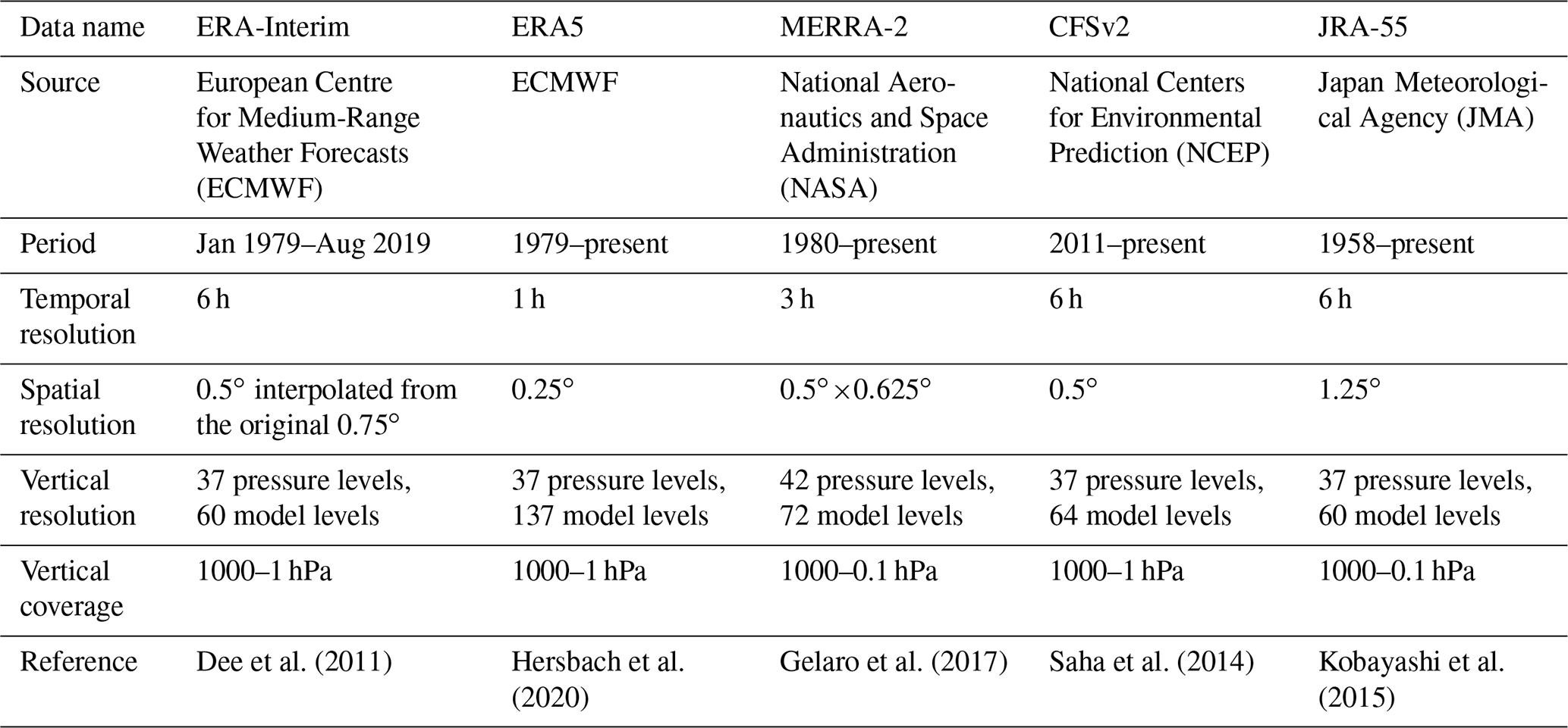
Reanalysis data were downloaded for a period covering the ACLOUD and PASCAL campaigns. To detect the ARs, specific humidity, temperature, and meridional and zonal components of the wind were acquired from 1000 to 300 hPa. Except for MERRA-2, all reanalyses were downloaded for 20 pressure levels, with vertical steps of 25 hPa, from 1000 to 750 hPa, and vertical steps of 50 hPa onwards. In the case of MERRA-2, the variables were downloaded for 21 pressure levels, from 1000 to 700 hPa, with vertical steps of 25 hPa, and from 650 hPa onwards, with vertical steps of 50 hPa. As the majority of the reanalysis datasets, with the exception of MERRA-2, have the first pressure levels below the surface, we applied a procedure similar to Gorodetskaya et al. (2020) that uses the variable surface pressure to exclude these layers. To ensure a full assessment of the events, mean sea level pressure, potential temperature (at 2 potential vorticity units – PVU), geopotential (at 700 hPa), sea-ice area fraction, total precipitation, and snowfall data were also obtained.

2.3 Regional climate model

The detected ARs and related precipitation were compared to the output of the state-of-the-art atmospheric regional climate model HIRHAM5 (Christensen et al., 2007; Sommerfeld et al., 2015), which participated in recent model intercomparisons within Arctic CORDEX (Inoue et al., 2021; Sedlar et al., 2020). Furthermore, HIRHAM5 has been thoroughly evaluated and applied for a wide range of Arctic climate studies, which include, for example, the quantification of the freshwater input in south-west Greenland (Langen et al., 2015), cyclone activity in the Arctic (Akperov et al., 2018), Arctic 2 m air temperature (Zhou et al., 2019), and clouds and radiation processes over the Arctic Ocean (Inoue et al., 2021; Sedlar et al., 2020).

This model includes the physical parameterizations of the general circulation model ECHAM5 (Roeckner et al., 2003). Relevant for this paper, the stratiform cloud scheme consists of prognostic equations for the vapour, liquid, and ice phase respectively; a cloud microphysical scheme (Lohmann and Roeckner, 1996); and a diagnostic relative-humidity-based cloud cover scheme (Sundqvist et al., 1989). For precipitation, all relevant microphysical processes and conversions are parameterized; for details, we refer the reader to Roeckner et al. (2003).

The applied domain comprises the entire Arctic for latitudes higher than approximately 65^∘ N, with a horizontal resolution of 0.25^∘ and 40 vertical levels until 10 hPa and 10 vertical levels in the lowest first kilometre. A more detailed description of the model and its parameterizations can be found in the given references.

ERA-Interim was used to initialize and force HIRHAM5. ERA-Interim fields are used as the lower boundary conditions, namely daily sea surface temperature and sea-ice concentration and the 6 hourly lateral boundary forcing for the prognostic variables (surface pressure and profiles of air temperature, horizontal wind components, specific humidity, cloud water, and ice). A grid point nudging (e.g. Omrani et al., 2012) was applied with a relaxation scale equivalent to a 1 % nudging in all model levels to constrain the large-scale dynamics.

3 Methodology

3.1 IWV and IVT

IWV and IVT were calculated for the entire duration of the ACLOUD and PASCAL campaigns, between the first near-surface level (equal to or less than 1000 hPa) and 300 hPa. IWV is derived from specific humidity (q) based on the following equation:

$$\begin{array}{}\text{(1)}& \mathrm{IWV}=-{\displaystyle \frac{\mathrm{1}}{g}}{\int }_{\mathrm{1000}\mathrm{hPa}}^{\mathrm{300}\mathrm{hPa}}q\mathrm{d}p,\end{array}$$

where g is the acceleration due to the gravity. IVT is based on q and horizontal wind (V) as follows:

$$\begin{array}{}\text{(2)}& \mathbf{IVT}=-{\displaystyle \frac{\mathrm{1}}{g}}{\int }_{\mathrm{1000}\mathrm{hPa}}^{\mathrm{300}\mathrm{hPa}}q\mathit{V}\mathrm{d}p.\end{array}$$

3.2 Detection of atmospheric rivers

The AR detection consists of applying tracking algorithms defined by specific criteria, such as minimum areas, with specific width and length, where IWV and/or IVT reach or exceed specific threshold values. Shields et al. (2018) presented an extensive list of tracking algorithms, with different criteria to identify ARs. The majority of the algorithms are applied on the western US (e.g. Dettinger, 2013; Gershunov et al., 2017; Rutz et al., 2014). Only few tracking algorithms were developed and applied for the polar regions, specifically to Antarctica (Gorodetskaya et al., 2014, 2020; Wille et al., 2019), and Greenland (Mattingly et al., 2018).

Two tracking algorithms were used to identify ARs: the Gorodetskaya et al. (2014, 2020) algorithm, developed and applied for Antarctica, and the Guan et al. (2018) global algorithm. Gorodetskaya et al. (2014) determined an AR when IWV (calculated from 900 to 300 hPa) is equal to or higher than a minimum threshold value near the Antarctic coast (within the 20^∘ W and 90^∘ E longitudinal sector) and continuous at all latitudes for at least 20^∘ equatorward (length >2000 km) within a limited width of 30^∘ longitude (∼ 1000 km at 70^∘ S increasing equatorward). This zonal mean threshold is based on saturated IWV and on an AR coefficient that determines the strength of the AR, which is explained in detail by Gorodetskaya et al. (2014). A second version of the algorithm included some updates, namely the computation of IWV from the first near-surface level with pressure equal to or less than 1000 to 300 hPa and the longitude width of 40^∘ in order to include zonally oriented ARs (Gorodetskaya et al., 2020).

We adapted this formulation for the Arctic, considering the ARs reaching and crossing 70^∘ N (within the 50^∘ W and 110^∘ E longitudinal sector, according to the considered campaign domain) and continuous at all latitudes for at least 2000 km within a maximum width of 40^∘ longitude. The axis of an AR is defined as the maximum value of IWV at each latitude. In this study, we explored the sensitivity of the AR identification in the Arctic to both the threshold and various geometric criteria and have also included the potential AR events (pAR) when IWV is equal to or higher than the threshold (as defined in Gorodetskaya et al., 2020). If the geometrical criteria are also met, this event is classified as an AR. This algorithm will be hereafter referred as “Gorodetskaya2020”. ERA-Interim, ERA5, CFSv2, MERRA-2, and JRA-55 reanalysis were used to identify pARs and ARs, whereas the HIRHAM5 model was only used to identify pARs, due to its limitation with respect to spatial coverage (approximately north of 65^∘ N), both based on Gorodetskaya2020.

The second tracking algorithm, based on IVT, is fully described in Guan and Waliser (2015) (V1.0). In this case, the identification of an AR is based on several conditions. First, an IVT threshold for each grid cell is calculated, which results from the combination of a defined percentile and a fixed lower limit value. As the polar regions are characterized by low values of IVT, mainly due to lower moisture values, the threshold is defined using the 85th percentile and a lower limit value of 100 kg m⁻¹ s⁻¹. If the objects exceed this limit, the IVT direction is evaluated such that the coherence in IVT direction, the object mean meridional IVT, and the consistency between object mean IVT direction and overall orientation are checked. A filter for the length (minimum 2000 km) and the length / width ratio of each object (higher than 2) is then applied.

In this study, we used a refined version of this tracking algorithm, described in Guan et al. (2018) (V2.0), which, instead of applying a fixed IVT threshold (85th percentile), includes the application of successively increasing IVT percentile thresholds (from the 85th to 95th percentile, by 2.5 percentile steps). This algorithm will be referred as “Guan2018” in the following sections. Only MERRA-2 reanalysis, covering a period from 1980 to 2019, was used to calculate IVT and to detect the ARs based on Guan2018. This database was provided by Bin Guan (https://ucla.box.com/ARcatalog; Guan, 2017).

3.3 Air mass trajectories

The HYbrid Single-Particle Lagrangian Integrated Trajectory (HYSPLIT) back trajectory model from the National Oceanic and Atmospheric Administration (NOAA) (Draxler and Hess, 1998) was used in order to track multiple air masses and establish possible moisture sources. This model computes simple air parcel trajectories, complex transport, dispersion, chemical transformation, and deposition simulations (Rolph et al., 2017; Stein et al., 2015), based on gridded meteorological data archives. For this study, we used the NCEP Global Data Assimilation System (GDAS) model with a horizontal resolution of 0.5^∘. Amongst the datasets available from the online platform, this was the most suitable for our study due to its finer spatial resolution. The dates when the ARs reached Ny-Ålesund were used to compute an ensemble of 5 d back trajectories with 27 members. The calculation of each member consists of adding an offset to the meteorological data (one grid point and 0.01 sigma units in the vertical).

4 Results

4.1 AR detection during the ACLOUD and PASCAL campaigns

A synoptic overview of ACLOUD and PASCAL has been presented by Knudsen et al. (2018) in which four events with substantial water vapour transport were identified: the 30 May event, the 6 June event, the 9 June event, and the 13 June event (see their Fig. A1). Here, we take a closer look at these events using high-temporal-resolution IWV measurements by HATPRO in Ny-Ålesund and using IWV and IVT from the ERA5 reanalysis during the complete period of the ACLOUD and PASCAL campaigns; the latter data depict strong IWV and IVT variability including distinct IWV maxima on these days (Fig. 1). Following this, these events and their possible association with ARs are analysed.

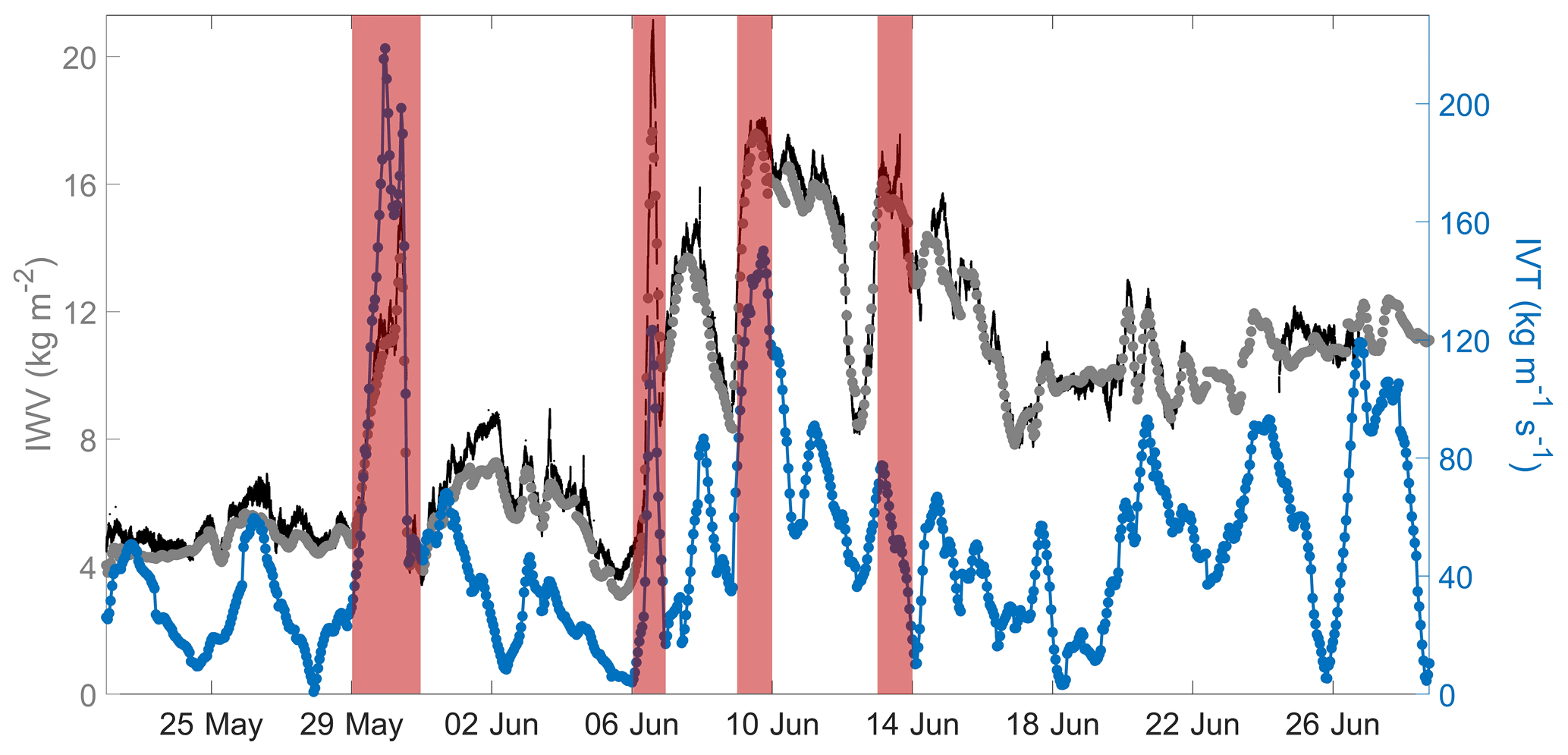
Figure 1 Time series of integrated water vapour (IWV, kg m⁻²), based on HATPRO measurements at Ny-Ålesund (black line) and ERA5 reanalysis at the closest grid (grey dots), and integrated vapour transport (IVT, kg m⁻¹ s⁻¹, blue dotted line), based on ERA5 reanalysis, for the ACLOUD and PASCAL campaigns (22 May–28 June 2017). Red bars show anomalous IWV and/or IVT at Ny-Ålesund.

For the times of the highest IWV at Ny-Ålesund during each event, we investigate the spatial IWV structure for three reanalysis datasets (ERA-Interim, ERA5, and MERRA-2) with different temporal and spatial resolution, HIRHAM5 model, and satellite measurements (Fig. 2). To find which events were identified as pARs or ARs, the Gorodetskaya2020 tracking algorithm was applied to the reanalysis and model fields. Note that polar orbiting satellite measurements with limited swath width are not suitable to detect ARs because the application of the tracking algorithms implies using a complete gridded data. The ARs detected by the Guan2018 database (only applied to MERRA-2 reanalysis) were also included to compare the differences between both tracking algorithms. The area covered by these pARs or ARs and the periods 24 h before and after these times are shown in Fig. 3.

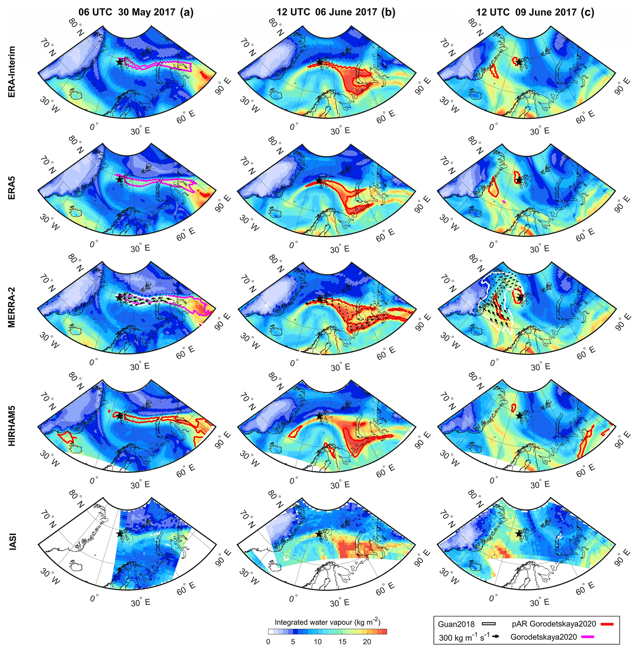
Figure 2 Maps of the integrated water vapour (IWV, kg m⁻², coloured shading) for the times with the highest IWV values in Ny-Ålesund during the 30 May event (first column, a), the 6 June event (second column, b), and the 9 June event (third column, c) based on reanalyses (ERA-Interim, ERA5, and MERRA-2), the HIRHAM5 model, and IASI observations. The magenta line shows the AR shape (based on Gorodetskaya2020), and the red line shows the shape of pARs (IWV≥IWV_thres, based on Gorodetskaya2020). The white line shows the AR shape (based on Guan2018), and black arrows show the integrated vapour transport (IVT, kg m⁻¹ s⁻¹), both based only on MERRA-2 reanalysis. Note that the AR shape based on Gorodetskaya2020 might overlap with the pAR shape in some cases. The black star shows the Ny-Ålesund location. Figures S1, S2, and S3 show the complete temporal evolution of the events for all datasets.

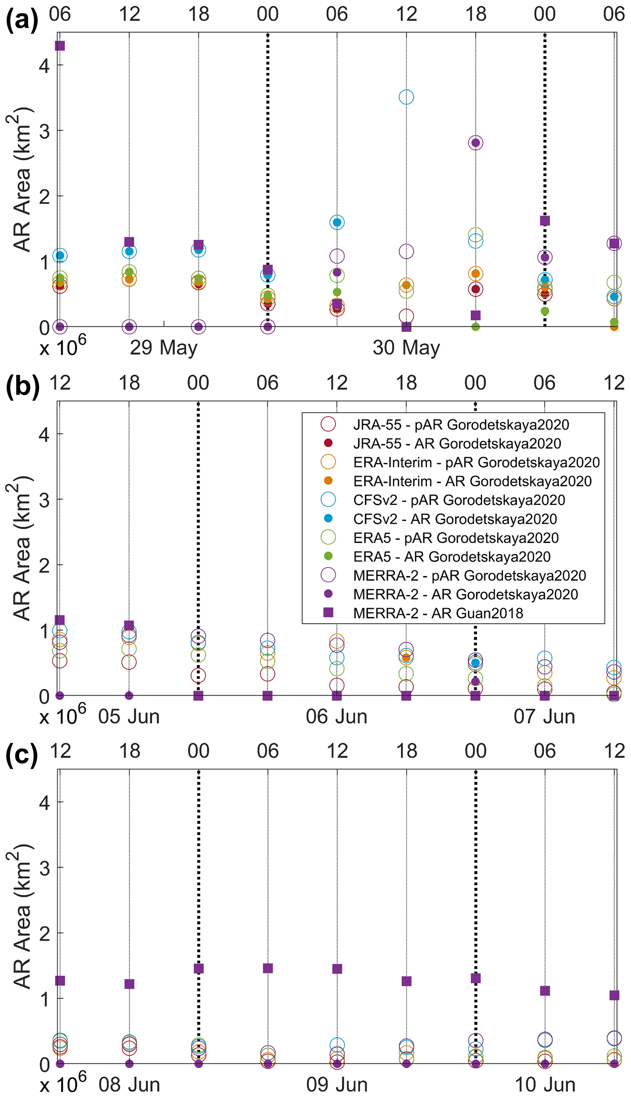
Figure 3 Time series of the area of the AR shape (based on Gorodetskaya2020), of the shape of pARs (IWV≥IWV_thres, based on Gorodetskaya2020), and of the AR shape (based on Guan2018, only for MERRA-2 reanalysis) during the 30 May event (a), the 6 June event (b), and the 9 June event (c) based on reanalyses (ERA-Interim, MERRA-2, ERA5, CFSv2, and JRA-55).

After applying the Gorodetskaya2020 tracking algorithm, two of the four events were detected as pARs: 30 May and 6 June (Fig. 2a, b – red lines; Fig. 3a, b – coloured circles). With the inclusion of the geometrical criteria, only the first event was identified as an AR (Fig. 2a – magenta line; Fig. 3a – coloured dots), as the current geometrical criteria prevent the 6 June event from being identified as an AR (explained later). The Guan2018 detection algorithm identified two ARs on 30 May and 9 June (Fig. 2a, c – white lines; Fig. 3a, c – purple squares). The fourth event, on 13 June, was not identified by any tracking algorithm as an AR (and, thus, is not shown in this paper).

The first event, on 30 May, identified as an AR by both tracking algorithms, was associated with a long and narrow band with high IWV extending westward from western Siberia (around 60^∘ N, 90^∘ E) to the Svalbard archipelago (around 80^∘ N, 15^∘ E) (Fig. 2a). The AR had a similar shape in all reanalysis datasets, although it extended further south-east in MERRA-2 and CFSv2 products, which was possibly related to higher values of IWV in these reanalyses over the region (Fig. S1 in the Supplement), resulting in a larger area covered by the pAR and AR shapes (Fig. 3a). Focusing only on MERRA-2 reanalysis in order to compare the two algorithms, both show overlapping contours (Fig. 2a). While the Gorodetskaya2020 shape was more elongated and extended to lower latitudes, until continental Siberia, covering a larger area (Fig. 3a), the Guan2018 shape was confined to the ocean area due to lower values of IVT over land (not shown in the paper).

One week later, on 6 June, the second event identified as a pAR by Gorodetskaya2020 made landfall in Ny-Ålesund (Fig. 2b). This AR resulted from two long and narrow filaments with high IWV, also extending from western Siberia, converging into one wider filament near Novaya Zemlya. The pAR shape was similar in ERA-Interim and ERA5, but it extended further south-east for MERRA-2 and CFSv2 due to the higher values of IWV over continental Siberia compared with ERA-Interim, ERA5, and JRA-55 reanalyses (Fig. S2). No major differences were noticed in the area of the pAR/AR shapes (Fig. 3b). Events like this, with a strong zonal component, are not identified as ARs by both algorithms due to limitations in the definition of the tracking algorithm; however, the Gorodetskaya2020 algorithm identifies it as pAR before applying geometrical criteria. Due to the strong zonal component and complex shape of this pAR, the event was not identified as a full AR by the strict geometrical criteria in the Gorodetskaya2020 algorithm. Currently the geometric criteria in the Gorodetskaya2020 algorithm are being adapted such that zonal events must be taken into account in future studies when applying this and other algorithms to long-term analysis.

Three days later, on 9 June, the third event was identified by the Guan2018 tracking algorithm as an AR, whereas it did not fulfil the criteria defined by the Gorodetskaya2020 algorithm. Although small pAR areas were also identified using the latter algorithm, as there was no consecutive shape inferred, the adaptation of the geometrical criteria used in the algorithm would still not include these areas as a full AR (Figs. 2c, 3c). Note that the Guan2018 global algorithm is generally much less restrictive than the polar-specific algorithms (Rutz et al., 2019). In the case of this event, this might be due to the lower values of IWV, which compromise the identification of the event as an AR by Gorodetskaya2020, and high IVT values in coastal Greenland (not shown), which allowed the identification of the event as an AR by Guan2018. However, the use of a different type of threshold to identify ARs might play an important role in the restrictiveness of the algorithms. In the case of Guan2018, which is based on an absolute threshold (based on percentiles), it can be less restrictive in the polar regions than Gorodetskaya2020, which is based on a zonal mean threshold of saturated IWV, that seems to be more suitable to identify ARs in polar regions. This event reached Ny-Ålesund extending north-westward from the north-eastern Atlantic (near the Scandinavian Peninsula) towards Greenland, passing over the north-eastern region of Greenland, and then turning south-eastward before eventually reaching Svalbard from the north. A similar IWV pattern was found in all reanalyses.

These bands of high IWV were observed in all reanalysis datasets and the HIRHAM5 model, despite some differences in the amount of IWV and in the shape of the pARs and ARs. These discrepancies might be related to different spatial and temporal resolutions as well as data assimilation of the reanalysis products and the model. In general, the comparison of the reanalysis datasets and the HIRHAM5 model with IASI measurements shows similar amounts and locations of the bands of high moisture content. A more quantitative assessment of different IWV datasets including further satellite products has been carried out by Crewell et al. (2021).

The complete spatio-temporal evolution of the three events, including the maps for 6 h before and after the IWV peaks and all of the reanalysis products, is shown in Figs. S1, S2, and S3. Comparing the events, the first two events extended from western Siberia, whereas the last event extended from Scandinavia; however, despite these differences, the three events were intense short-duration events.

In the following sections, we provide a detailed analysis of the three events detected as pARs/ARs.

4.2 Synoptic conditions during ARs affecting Svalbard

To understand which meteorological conditions triggered the detected events (pARs and ARs), we performed a detailed analysis of the synoptic conditions using ERA5 reanalysis, due to its high temporal and spatial resolution.

Figure 4 (Figs. S4 and S5 for temporal evolution) shows the mean sea level pressure (MSLP), the geopotential height at 700 hPa, and potential temperature (θ) at 2 PVU, which is commonly used to define the height of the dynamical tropopause (Hoskins et al., 1985; Juckes, 1994; Wilcox et al., 2012; Woollings et al., 2018), providing an analysis of the upper-level flow. The combination of these variables is used to study the atmospheric blocking, which has previously been associated with ARs (Benedict et al., 2019; Francis et al., 2020; Rabinowitz et al., 2018; Wille et al., 2019). Atmospheric blocking leads to persistent weather conditions, playing an important role in directing ARs poleward. This phenomenon has a wide range of consequences, ranging from persistent high/low temperatures to hydrological impacts (Woollings et al., 2018). Knudsen et al. (2018) mentioned that moderate negative Arctic Oscillation index values were found, which are related to more frequent blocking high-pressure events, during the warm period of the ACLOUD and PASCAL campaigns (from 30 May to 12 June).

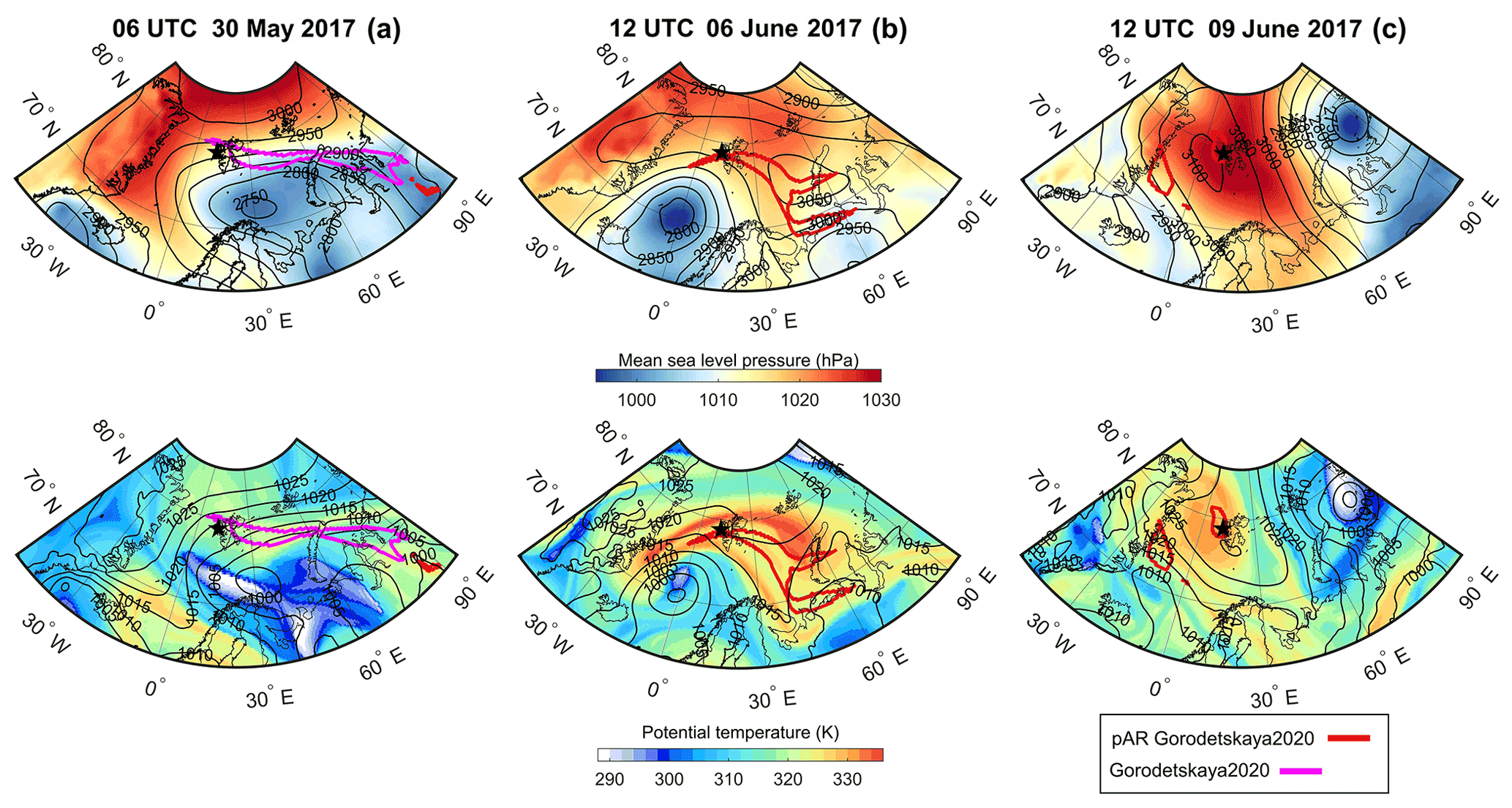
Figure 4 Maps of mean sea level pressure (hPa, coloured shading) and geopotential height at 700 hPa (m, contours) (top row) and maps of potential temperature at 2 PVU (K, coloured shading) and mean sea level pressure (hPa, contours) (bottom row) based on ERA5 reanalysis during the peak of the 30 May event (a), the 6 June event (b), and the 9 June event (c). The magenta line shows the AR shape (based on Gorodetskaya2020), and the red line shows the shape of pARs (IWV≥IWV_thres, based on Gorodetskaya2020). The black star shows the Ny-Ålesund location. Figures S4 and S5 show the complete temporal evolution of the synoptic conditions during the events.

During the first event, a low-pressure system was centred over the Barents Sea, with a blocking high-pressure ridge in the polar latitudes (Fig. 4a). These systems remained almost stationary, although the cyclone moved slightly south-westward and weakened (Fig. S4a). Simultaneously, low potential temperatures were found in the location of the low-pressure system (Fig. S5a), as expected, following the slow cyclone propagation south-westward (Fig. S4a). In the region of the AR, relative high values of potential temperatures were noticed, associated with the vertical advection of potential temperature (Fig. S5a). This displacement directed the moisture transport and the associated AR westward from the lower latitudes in Siberia towards higher latitudes around Svalbard, followed by a small shift in the south-westward direction.

One week later, a stronger low-pressure system affected the southern region of the Svalbard archipelago along with a high-pressure system at higher latitudes; this was less pronounced than the previous event (Fig. 4b). The cyclone progressed north-westward from northern Scandinavia and slowly moved towards Greenland with no intensity changes (Fig. S4b). At the same time, a second weaker low-pressure system located in northern Russia caused the tilt of one of the pAR branches in a zonal direction. These near-stationary systems, associated with atmospheric blocking, directed the moisture transport from western Siberia to southern Svalbard. In the region of the pAR and north of its shape, even higher potential temperature values were found than in the previous AR (Fig. S5b).

Three days later, a low-pressure system was located over the Kara Sea, while a high-pressure system was centred over Svalbard with decreasing pressure values towards Greenland (Fig. 4c), where the AR only identified by Guan2018 was located (Fig. 2c). Again, the pressure systems remained almost stationary, propagating slowly north-eastward (Fig. S4c) and leading to the curvature of the AR from northern Greenland towards northern Svalbard (Fig. S3c). In the meantime, high potential temperature values were found from the Scandinavia Peninsula to the coast of Greenland, along the shape of the AR (Fig. 4c), which were more intense in the region of the AR tilt towards Svalbard. These values slowly decreased with increasing curvature of the AR towards Svalbard (Fig. S5c).

4.3 AR impacts at Svalbard

4.3.1 Variability of IWV and IVT

After analysing the spatio-temporal evolution of the events, it is also important to investigate them at a local scale. An analysis of the ARs focusing on Ny-Ålesund was performed using all reanalysis datasets in synergy with in situ measurements (radiosonde), ground-based remote sensing (HATPRO and GNSS), satellite-based measurements (IASI L2 PPFv6), and the HIRHAM5 model. From the reanalyses and model, the nearest grid point to Ny-Ålesund is used for the comparison with the station data. The landfall time is based on the IWV peaks in Ny-Ålesund (06:00–12:00 UTC on 30 May and 12:00 UTC on 6 and 9 June).

Firstly, we assessed the temporal evolution of the IWV and IVT during the events (Fig. 5). Further information about the root mean square error (RSME) and bias between the reanalyses, observations, and model is shown in Table S1. We used the radiosondes as a reference (6 h steps) for a 48 h period (24 h before and after the AR reached Ny-Ålesund). On the day before the arrival of the first event at Ny-Ålesund, the measurements, reanalyses, and model showed low IWV and IVT values, which slowly increased until the beginning of the next day (Fig. 5a). During the first 6 h, the IWV continued to increase slowly. Conversely, radiosondes showed a slight decrease in IVT, which was not represented by the MERRA-2 reanalysis and HIRHAM5 model. During landfall (between 06:00 and 12:00 UTC), there was a slight increase in IWV from 11 to 15 kg m⁻², which was missed by the ERA-Interim, CFSv2, and JRA-55 reanalysis, due to low temporal resolution (6 h), along with an increase in IVT. Both IVT peaks were poorly represented by the reanalyses, with the exception of ERA5 (Table S1, smaller bias). After landfall, IVT and IWV decreased sharply, which was properly represented by all datasets.

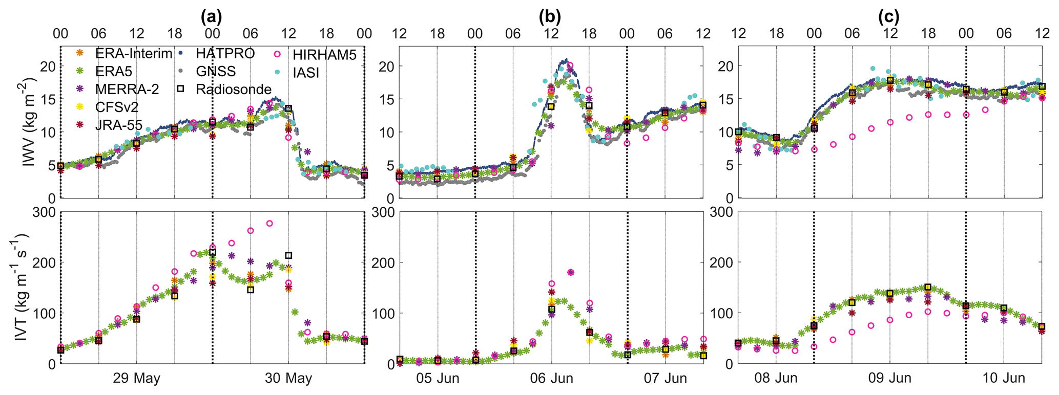
Figure 5 Time series of integrated water vapour (IWV, kg m⁻², top row) and integrated vapour transport (IVT intensity, kg m⁻¹ s⁻¹, bottom row), based on reanalyses (ERA-Interim, ERA5, MERRA-2, CFSv2, and JRA-55), radiosonde, ground-based remote sensing (HATPRO and GNSS) and satellite measurements (IASI), and the HIRHAM5 model, at Ny-Ålesund during the 30 May event (a), the 6 June event (b), and the 9 June event (c).

On the day prior to the landfall of the second event, persistent low values of IWV and IVT were represented by all datasets (Fig. 5b). During the 6 h before the maximum IWV occurred at Ny-Ålesund, IWV and IVT sharply increased from 6 to about 20 kg m⁻² and from 5 to more than 120 kg m⁻¹ s⁻¹ respectively (Table S2, IWV and IVT amplitude). The IWV and IVT peaks lasted around 12 h. For IWV, the peak was misrepresented by CFSv2, JRA-55, ERA-Interim, and the radiosondes due to the low temporal resolution of 6 h, whereas similar behaviour to the first event could be noted for the IVT peak, with an overestimation of MERRA-2 and HIRHAM5 (Table S2, IVT integrated during the event). IVT differences can amount to up to 35 % (between ERA5 and MERRA-2) during the phase of decreasing IVT.

On the day prior to the third event, a slight decrease in IWV and IVT was noticed in all datasets, with the exception of MERRA-2 (Fig. 5c). High IWV and IVT values were observed during the whole day of the event, even after landfall, although the HIRHAM5 model underestimated these values by up to 55 % when compared with the radiosondes (Table S1). A previous study by Sedlar et al. (2020) showed large IWV biases based on the HIRHAM5 model for events with strong IWV. On the following day, IVT slowly decreased, whereas IWV remained unchanged. Contrary to the previous events, no prominent peak in IWV or IVT was observed.

For all the events, ERA5 seems to more realistically represent the maximum and minimum values of IWV and IVT, when compared with GNSS, HATPRO, and radiosondes (Table S1), due to its high temporal and spatial resolution. Note that even amongst the observation datasets there are minor differences (Table S1). However, previous studies showed that IWV differences are not significant in Ny-Ålesund with an RMSE lower than 1 kg m⁻² (Nomokonova, 2020).

During the first two events, the periods when the HIRHAM5 model overestimated the IVT might be explained by changes in the wind components, as the HIRHAM5 results were similar to the reanalyses and observations for IWV (based on the specific humidity). An analysis of the spatial evolution of IVT based on HIRHAM5 and ERA-Interim (which was used to force the model) showed some differences in the IVT values, which were higher in the HIRHAM5 model (Figs. S6, S7). As the beginning of the edge of the band of high IVT is located around Ny-Ålesund in the first event (Fig. S6) and the end of this band is located near Ny-Ålesund in the second event (Fig. S7), a minor difference in its location (e.g. due to slight shifts of the low- and high-pressure systems) induces large changes in IVT at Ny-Ålesund.

4.3.2 Variability of vertical profiles of humidity and wind

The vertical structure of the ARs is also an important component when studying these types of events. Figure 6 shows the vertical profiles of specific humidity and wind speed, based on reanalyses, radiosonde measurements, and the HIRHAM5 model, during the peaks of the events in Ny-Ålesund. The complete temporal evolution of the vertical profiles is presented in Fig. 7 and in Figs. S8 and S10 in the Supplement. For an easier comparison of the performance of each dataset, the bias and RMSE between each reanalysis and model and the radiosondes are shown in Fig. S9.

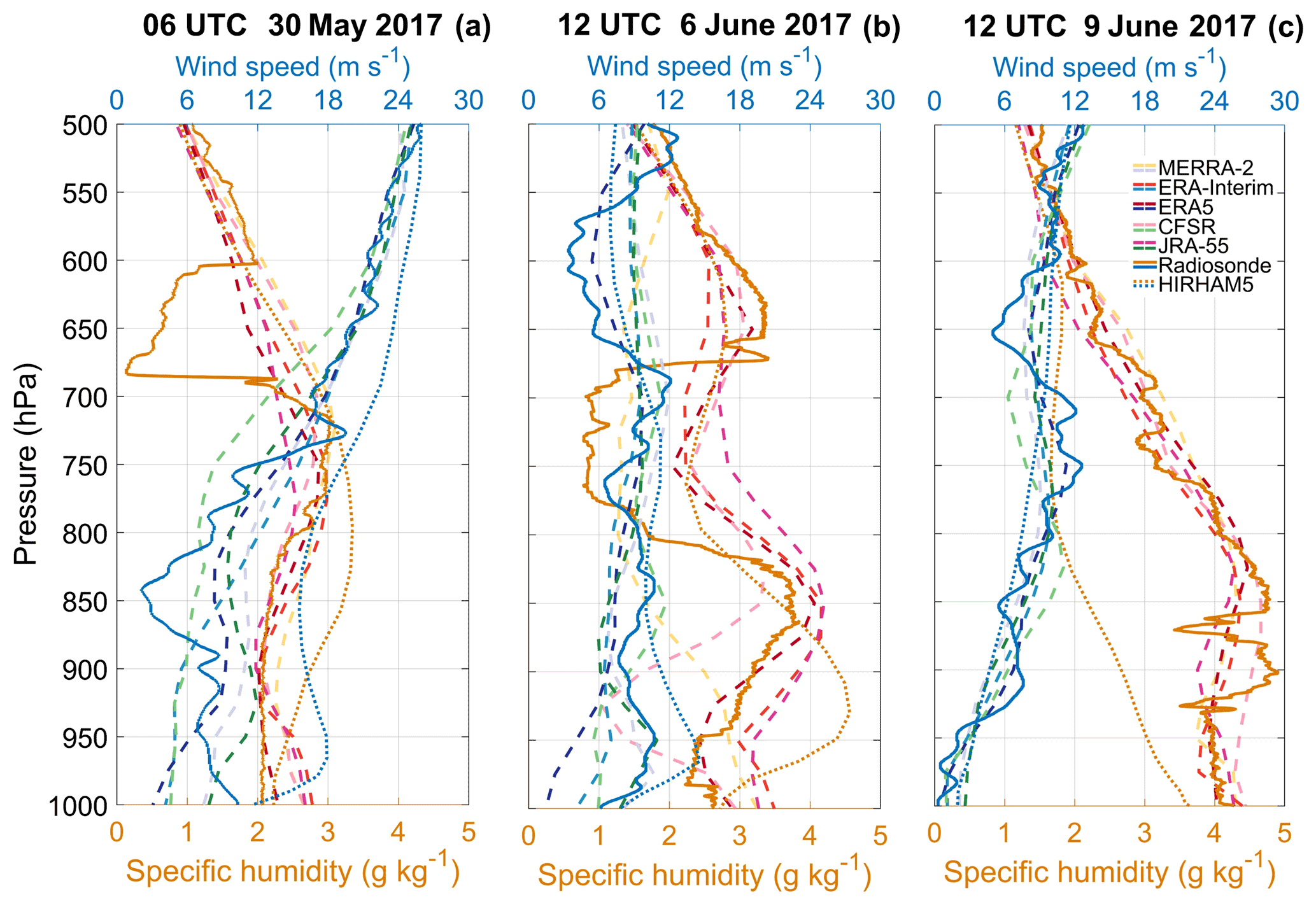
Figure 6 Vertical profiles of specific humidity (g kg⁻¹, pink/orange colours) and wind speed (m s⁻¹, blue/green colours) at Ny-Ålesund, based on radiosonde (solid lines), reanalyses (ERA-Interim, ERA5, CFSv2, JRA-55, and MERRA-2; dashed lines), and the HIRHAM5 model (dotted lines), during the 30 May event (a), the 6 June event (b), and the 9 June event (c). Figure S8 shows the complete temporal evolution of the vertical profiles, and Figure S9 shows the bias and RMSE of each reanalysis and model compared to the radiosondes (reference).

During the first event, on 30 May, the radiosonde shows a layer of enhanced specific humidity between 1000 and 700 hPa, which was overestimated by the HIRHAM5 model (Figs. 6a, S8a, S9). This layer was followed by a dry layer until 600 hPa, which was only captured by the radiosonde. Wind speed values were not well represented from the surface until 650 hPa by all of the reanalyses when compared with the radiosonde, as a difference of a factor of 2 occurs at some levels. The HIRHAM5 model largely overestimated the wind speed values along the entire column, with differences varying from 15 % at 1000 hPa, to around 80 % at 850 hPa, and, finally, to almost 0 % at 500 hPa.

One week later, on 6 June, with the approach of the second event, a complex vertical structure with two maxima in specific humidity of about 4 g kg⁻¹ at 850 hPa and 3.5 g kg⁻¹ at 650 hPa with a pronounced dry layer with less than 1 g kg⁻¹ was observed by the radiosondes. However, compared with the first event, where all datasets failed to reproduce the dry layer, the reanalyses and model show a dry layer here, although it is much weaker when compared with the radiosondes. It is possible that, in this case, the formation of the dry layer was explained by other mechanisms which the reanalyses were able to reproduce more accurately. Furthermore, below this layer, only ERA5 represented similar values of specific humidity to the radiosondes (Figs. 6b, S8b, S9): CFSv2 and MERRA-2 are too dry and the others are too wet, and CFSv2, MERRA-2, and HIRHAM5 strongly misinterpret the vertical profile. Compared with the first event, only minor differences were noticed in the wind speed, despite an overestimation from HIRHAM5 below 850 hPa (Fig. S9). A total of 6 h later, the dry layer was still present, with even lower values of specific humidity, and its base moved upwards (Fig. S8b). A study performed by Neggers et al. (2019) analysed data from radiosondes launched from the Polarstern research vessel during the period from 5 to 7 June 2017. In the above-mentioned study, similar dry layers were identified in western Svalbard on 6 June at 04:00 and 10:00 UTC at respective heights of around 2.5 and 2 km.

Three days later, during the third event, on 9 June, the radiosondes captured a layer with high specific humidity values of up to 5 g kg⁻¹ below 800 hPa, which was represented by all reanalysis datasets (Figs. 6c, S8c, S9). The HIRHAM5 model largely underestimated the specific humidity until 600 hPa and showed an unrealistic decrease in humidity with height. The wind speed profiles were properly represented by all datasets, with the calmest situation of all events in the lower tropopause.

The vertical profiles are in agreement with Fig. 5, as the reanalyses/model overestimation (underestimation) of specific humidity in some or all vertical levels lead to higher (lower) values of IWV. Furthermore, the overestimation of the HIRHAM5 wind speed during the first two events, mainly near the surface, and differences in the amounts of specific humidity might explain the major differences in HIRHAM5 IVT noticed in Figs. S6 and S7. Moreover, the underestimation of HIRHAM5 specific humidity in the last event explains the major differences in IWV and IVT observed in Fig. 5c.

The temporal evolution of specific humidity vertical profiles during the three events based on radiosondes, reanalyses, and the HIRHAM5 model is illustrated in Fig. 7. On the day prior to the first event, the radiosondes show low values of specific humidity. Associated with the approaching event, specific humidity showed a sharp increase, with a moist layer extending from the surface until 675 hPa with a peak around 800 hPa. These observations also captured a dry layer present above the moisture peak (from 700 to 600 hPa) at 06:00 UTC. Maximum moisture values were observed at 12:00 UTC and were followed by a sharp decrease. Overall, the height of the maximum increase in specific humidity (around 675 hPa) was well captured by all of the reanalyses and by the model, although MERRA-2 and CFSv2 (Fig. S10a) showed a more extended layer of moist air. Furthermore, JRA-55 and ERA-Interim showed lower amounts of specific humidity in the peak of the moisture layer (800 hPa; Fig. S10a). The dry layer was not properly represented by any of the reanalyses or the model, which might be due to its narrow vertical extent of about 85 hPa. It is also interesting to note that the observed reduced moisture within the whole column after the event is not fully realistic in the reanalyses; only ERA5 and HIRHAM5 also showed the reduction in the low layers near the surface.

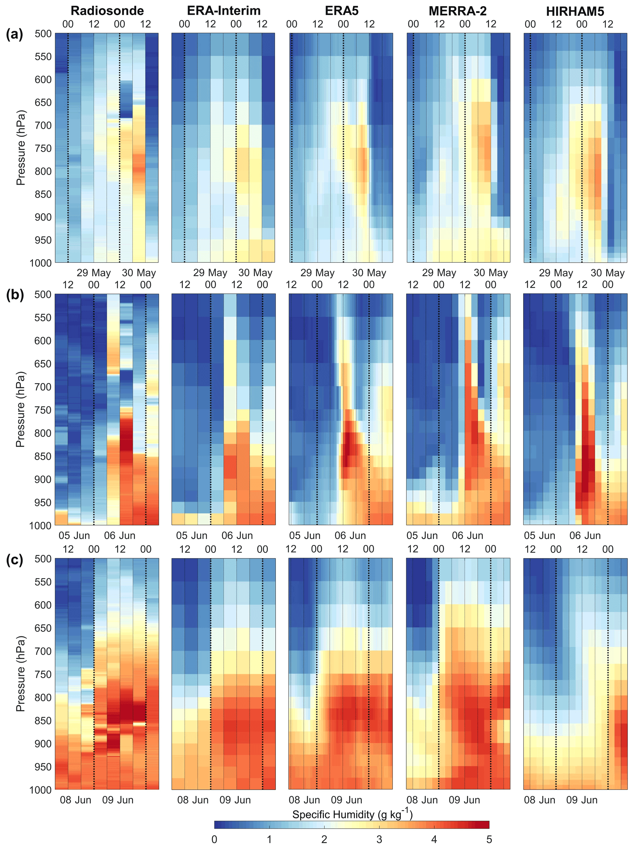
Figure 7 Temporal evolution of vertical profiles of specific humidity (g kg⁻¹) at Ny-Ålesund, based on radiosondes, reanalyses (ERA-Interim, ERA5, and MERRA-2), and the HIRHAM5 model, during the 30 May event (a), the 6 June event (b), and the 9 June event (c). Time steps on the x axis mark the end of the observations/reanalyses/model. Figure S10 shows all datasets.

One week later, a stronger moisture intrusion associated with the second event reached Ny-Ålesund. Before its approach, low specific humidity values were found, followed by an intense and rapid increase in moisture. Before the peak of the event, there was a moist layer from the surface until 800 hPa that was situated below a dry layer which extended until 700 hPa. At the peak, this moist layer extended upward until 750 hPa, followed by a sharp decrease in the moisture amount. By the end of the day, high amounts of specific humidity were still captured below 850 hPa in Ny-Ålesund. The reanalyses and model satisfactorily represented the timing and height of the elevated moisture intrusion associated with the event. Overall, the amount of specific humidity was well represented by the reanalyses and model, despite the underestimation by ERA-Interim, CFSv2, and JRA-55 (Fig. S10b). However, the dry layer was not captured well by the reanalyses or model, with the exception of the highest-resolution reanalysis, ERA5, which showed the moisture inversion, despite the fact that its intensity was strongly underestimated.

Two days later, high amounts of specific humidity were captured by the radiosondes below 800 hPa. On the following day, with the arrival of the third event, the moisture amounts increased and were accompanied by the expansion of the height of the maximum specific humidity until 650 hPa. After the event, high amounts of humidity were still noticed, and the height of maximum specific humidity remained unchanged until the following day. The reanalyses properly represented the height of maximum specific humidity, despite underestimating the amounts of specific humidity. The more pronounced differences were noticed in HIRHAM5 model, which misrepresented the height of maximum humidity and underestimated the amount of specific humidity. Previous studies by Inoue et al. (2021) and Sedlar et al. (2020) have shown that the largest specific humidity errors in HIRHAM5 occur across the mid-troposphere to lower troposphere, with the RMSE peak at around 850–925 hPa, which is in agreement with our results. Furthermore, Sedlar et al. (2020) showed that the bias of the vertical profiles of specific humidity vary temporally, and the largest values were found during events of warm, moist air intrusions.

4.4 Precipitation patterns during ARs

ARs are usually associated with intense precipitation events, which might occur in the form of rain or snow in the Arctic. Prior studies have associated extreme precipitation events with ARs in Svalbard (Kelder et al., 2020), with nearly half of the 15 largest precipitation events in Ny-Ålesund from 1979 to 2014 due to ARs (Serreze et al., 2015). Evidence of the influence of ARs on the sea-ice loss to the Arctic region has also been shown (Wang et al., 2020). However, an assessment of the sea-ice retreat or expansion mechanisms is beyond the scope of this study.

In this section, we performed a spatial analysis of the precipitation patterns related to the identified ARs as well as of the associated changes in the sea-ice edge using reanalysis data and the HIRHAM5 model (Fig. 8). The analysis was completed by the discrimination of the precipitation phase, in terms of snowfall and rainfall (Figs. 9, S11, S12, S13). This analysis was based on the accumulated amounts of precipitation during 48 h periods (24 h before and after the events reached Ny-Ålesund). A similar procedure was applied to the outline of the ARs that were previously identified by the tracking algorithms. Thus, the total AR shapes shown in Figs. 8, 9, and S11–13 correspond to the total area occupied by each pAR/AR shape during the 48 h periods (similar to precipitation), as these shapes moved and evolved during each event.

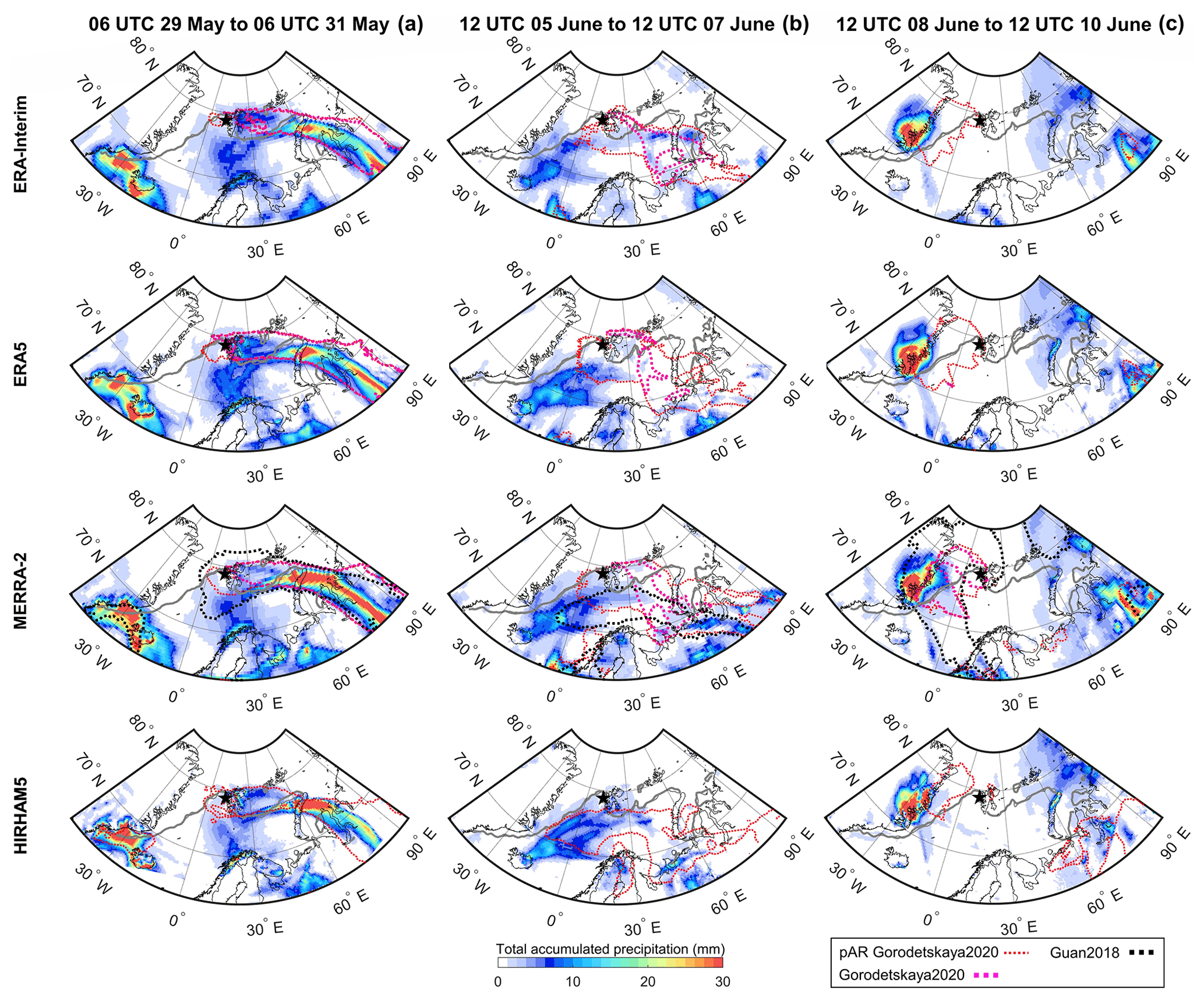
Figure 8 Maps of the total accumulated precipitation (mm, coloured shading) for the 30 May event (first column, a), the 6 June event (second column, b), and the 9 June event (third column, c) during a 48 h period (24 h before and after the AR reaches Ny-Ålesund, shown by the black star) based on reanalyses (ERA-Interim, ERA5, and MERRA-2) and the HIRHAM5 model. The grey lines show the sea-ice fraction using a 15 % threshold (the thin line represents 24 h before the event, and the thick line represents 24 h after the event). The magenta and red lines show the respective AR and pAR shapes based on Gorodetskaya2020. The black line shows the AR shape based on Guan2018 (available only for MERRA-2). Here, the AR shape lines encompass the total area of the ARs/pARs during the 48 h period. Figures S11, S12, and S13 show the discrimination of the precipitation phase (snowfall and rainfall) for all datasets.

Figure 9 Maps of the accumulated snowfall (mm, coloured shading, top row) and rainfall (mm, coloured shading, bottom row) for the 30 May event (a), the 6 June event (b), and the 9 June event (c) during a 48 h period (24 h before and after the AR reaches Ny-Ålesund, shown by the black star) based on ERA5 reanalysis. The grey lines show the sea-ice fraction using a 15 % threshold (the thin line represents 24 h before the event, and the thick line represents 24 h after the event). The magenta and red lines show the respective AR and pAR shapes based on Gorodetskaya2020. Here, the AR shape lines encompass the total area of the ARs/pARs during the 48 h period. Figures S11, S12, and S13 show the discrimination of the precipitation phase (snowfall and rainfall) for all datasets.

During the first event, all reanalyses show an enhanced band of precipitation within the pAR/AR shape from western Siberia to the Barents Sea (Figs. 8a, S11a). However, ERA-Interim and ERA5 show localized high values of precipitation (>25 mm accumulated during 48 h) in mainland Russia and in northern Novaya Zemlya and the adjacent region of the Kara Sea, whereas the MERRA-2, CFSv2, and JRA-55 reanalyses show a continuous band of high amounts of precipitation (maximum total precipitation values >40 mm during 48 h) from western Siberia extending through the Kara Sea to Novaya Zemlya (Figs. 8a, S11a). Simultaneously, the HIRHAM5 model has a similar pattern to the reanalyses, but high precipitation values are restricted to the Kara Sea and northern Novaya Zemlya (maximum precipitation of 90 mm during 48 h). This island, characterized by its high orography, mainly in the northern latitudes (maximum ∼ 1500 m), caused the orographic enhancement of precipitation. Thus, from Novaya Zemlya towards Svalbard, precipitation amounts were reduced, despite the fact that (depending on the reanalysis dataset) some smaller amounts of precipitation (<10 mm accumulated during 48 h) were noticed, and this might be mainly related to the föhn effect. Compared with the precipitation climatology of the Svalbard region (from 1979 to 2018) that varies from 31 mm at Svalbard Airport station, to 127 mm at Barentsburg station, and, finally, to 89 mm at Ny-Ålesund station and accumulated during spring (March to May) (Førland et al., 2020), the amount of precipitation reaching this region during the event is small. If we look at a monthly climatology of May in more detail (from 1951 to 1980), where precipitation at Barentsburg station was 25 mm during an average of 14 d (Aleksandrov et al., 2005), the amount of precipitation associated with the AR (accumulated over 2 d) was around 1 mm, which is less than the climatological amounts. The same climatology for Cape Zhelaniya station (northern region of Novaya Zemlya) shows that the average precipitation during May was 23 mm during 17 d (Aleksandrov et al., 2005), which, compared with the precipitation amounts verified in this region during the AR (in some datasets >10 mm during 2 d), shows that this event was more or less significant depending on the dataset (MERRA-2 provides a value of 11.7 mm during 2 d, corresponding to ∼ 50 % of the monthly climatological precipitation, and ERA5 provides a value of 0.3 mm during 2 d). For the Dikson Island station (located in northern Russia), the climatology shows an average precipitation of 26 mm during 18 d in May (Aleksandrov et al., 2005), while precipitation amounts reached 11.5 mm (MERRA-2 reanalysis) over 2 d during the AR, representing a significant amount of precipitation in this region (44 % of the climatological monthly precipitation). However, it is important to note that precipitation in this region in the ERA5 reanalysis was around 0.6 mm.

The majority of the precipitation was confined to the AR shape, but precipitation also occurred outside the AR associated with the extratropical cyclone in southern Svalbard. During this AR event, mixed-phase precipitation occurred, showing both snow and rain within the AR, and major differences were noticed across the reanalyses and model (Figs. 9a, S11b, S11c). ERA-Interim and JRA-55 were the only datasets with rainfall in the Svalbard region, whereas the CFSv2, MERRA-2, and ERA5 reanalyses as well as the HIRHAM5 model only showed rainfall in western Siberia and the adjacent coastal region (Fig. S11b). CFSv2 shows the highest amount of rainfall (>25 mm accumulated during 48 h) along western Siberia and a small portion of the Kara Sea during the 48 h period; ERA-Interim, MERRA-2, ERA5, and JRA-55 only have this amount of rainfall in the inner western Siberian region; and the HIRHAM5 model does not show such rainfall values in this region at all (Fig. S11b). Simultaneously, snowfall reached regions further north, extending from western Siberia towards Svalbard (Fig. S11c). The higher amounts of snowfall were noted in the Kara Sea and Novaya Zemlya (>40 mm during 48 h, with the exception of the ERA-Interim reanalysis), with their accentuated decrease north-westward of this island. The highest amounts of snowfall and rainfall were found in the southern part of the AR and south of the sea-ice edge in all datasets. However, smaller amounts of snowfall occurred over the sea ice, whereas rainfall was confined to regions south of the sea-ice edge, over the open sea, with the exception of ERA-Interim and JRA-55.

A full analysis of the total and mean precipitation amounts and discrimination of the precipitation phase within the pAR shape by Gorodetskaya2020 and within the AR shapes by Gorodetskaya2020 and Guan2018 is shown in Table 2. Overall, the area of the AR and pAR shapes was similar across all of the reanalyses. The exception was the AR shape by Guan2018, based on MERRA-2 reanalysis, which was more than 2 and 3 times larger than the respective pAR and AR shapes by Gorodetskaya2020 due to the different criteria used by the algorithms. These were associated with higher total amounts of total precipitation, mostly in the form of rainfall. Furthermore, one can notice that the AR shapes by Gorodetskaya2020 have higher mean values of total precipitation, rainfall, and snowfall than the pAR shapes, which is explained by the AR shapes being more restrictive, containing only higher amounts of precipitation. In particular, CFSv2 and JRA-55 show higher values of total and mean total precipitation, mainly due to higher values of rainfall when compared with the remaining reanalyses.

Table 2 Total and mean total precipitation, snowfall, and rainfall amounts within the pAR/AR shapes by Gorodetskaya2020 and Guan2018 (mm during 48 h) based on reanalyses (ERA-Interim, ERA5, MERRA-2, CFSv2, and JRA-55) during the 30 May 2017 event.

The sea-ice edge showed a retreat, mainly in the northern Barents Sea region north of Novaya Zemlya (Figs. 8a, S11), which might be explained by different mechanisms, such as high wind speed with a north-westward direction in the region of Novaya Zemlya, as mentioned previously (Figs. 2a, S1a, S6). This intense wind blowing over the limit of the sea-ice edge, which is defined by areas with at least 15 % ice cover, meaning it is already fragile, might have pushed the sea ice further north, causing its retreat.

Despite the similarities to the first event described in the previous sections, the second event, only 1 week later, on 6 June, was completely different in terms of precipitation patterns, with low amounts of precipitation within the AR shape (<15 mm accumulated over the 48 h period) (Figs. 8b, S12a). The majority of precipitation occurred south-west of the AR shape, directed towards Iceland, although precipitation occurred partially within the pAR shape in CFSv2 reanalysis, and the AR shape by Guan2018 extended more towards Iceland in MERRA-2 reanalysis, partially including precipitation, which was also noticed in the pAR shape by Gorodetskaya2020 in the HIRHAM5 model, including precipitation from this region (Figs. 8b, S12a). All reanalyses and the HIRHAM5 model show similar total precipitation patterns, although ERA-Interim has the lowest amounts of precipitation (maximum of 15 mm during 48 h south of the pAR/AR shapes). Most of the total precipitation occurred in the form of rain (Figs. 9b, S12b), with the exception of some areas where mixed-phase precipitation or only snowfall occurred (Figs. 9c, S12c), mainly near the coast of Greenland and in the north-east of Iceland. Precipitation mainly occurred over ice-free ocean with the exception of the area in south and east of Svalbard, where low values of rainfall were noted (<5 mm accumulated during 48 h), and reduced amounts of snowfall (<10 mm accumulated during 48 h) near the coastline of Greenland. No differences were noted in the sea-ice edge, possibly due to the reduced amounts of precipitation over the sea ice (rain or snow) and low values of IVT, and consequently wind speed, over the sea ice (Fig. S7).

During the third event, 3 days later, on 9 June, no precipitation was noticed in Svalbard, which was located at the edge of the pAR/AR (Fig. 8c). At the same time, high amounts of precipitation occurred on the east coast of Greenland, in the mountainous region of Scoresby Land (>20 mm accumulated during 48 h period), confined within the AR shape defined by Guan2018 and on the edge of the pAR shape defined by Gorodetskaya2020 algorithm. In this region, total precipitation amounts were similar in all reanalyses and the HIRHAM5 model (Fig. S13a); however, the discrimination of the precipitation phase shows major differences (Figs. 9c, S13b, S13c). With the exception of MERRA-2, all datasets show high amounts of rainfall in the coastal region of Greenland, over the sea ice (maximum of 64 and 110 mm during 48 h in the JRA-55 reanalysis and the HIRHAM5 model respectively), and high amounts of snow in the adjoining continental area (maximum of 80 and 200 mm during 48 h in the CFSv2 reanalysis and the HIRHAM5 model respectively). MERRA-2 presents low values of rainfall in coastal Greenland (maximum of 11 mm during 48 h) and high amounts of snow in the continental and coastal regions (maximum of 75 mm during 48 h). As observed in the last event, there were no major changes in the sea-ice extent.

A previous study by Boisvert et al. (2018) pointed to major differences in the precipitation amount and phase over the Arctic Ocean among eight reanalyses datasets, in which ERA-Interim, MERRA-2, and JRA-55 (analysed in our study) are included. The largest annual differences were found in East Greenland, the Kara Sea, and the Barents Sea, which might be explained by the influence of the storm track and how the reanalyses assimilate those events. The monthly analysis of the cumulative precipitation during May and June over this region shows no major discrepancies between the three reanalyses used in our study. The discrimination between snowfall and rainfall showed large differences amongst the reanalyses. As observed in our study, MERRA-2 showed higher amounts of snowfall over the Barents and Kara seas and coastal Greenland in comparison with ERA-Interim and JRA-55. The variability of rainfall between reanalyses is larger along the east coast of Greenland, and, as in our study, MERRA-2 has the lowest amounts of rainfall compared with the other reanalyses.

Finally, we performed an analysis of the air mass trajectories during the AR events using the HYSPLIT model (Fig. S14). The start date to calculate an ensemble of the back trajectories for the 5 previous days was defined based on the IWV peaks in Ny-Ålesund (06:00 UTC on 30 May and 12:00 UTC on 6 and 9 June). The trajectories were initiated at 800 hPa height at Ny-Ålesund. During the first AR, the trajectories showed low variance until 24 h prior to the initial date, with a mean trajectory path over the Barents and Kara seas before reaching the Ny-Ålesund site. Over the continent, the trajectories showed a higher variability, with the majority of the variability being confined to western Siberia (Fig. S14 – left panel). The second event showed that the majority of trajectories passed over the Kara and Barents seas before reaching Svalbard. After reaching the continent over western Siberia, some trajectories passed over the Baltic Sea, but the majority were limited to the region west of the Ural Mountains (Fig. S14 – middle panel). Few trajectories showed Greenland and northern Canada as a possible air mass path. The last event had a distinct behaviour, with the air mass trajectories passing over the Norwegian and Greenland seas before reaching Ny-Ålesund (Fig. S14 – right panel). The trajectories extended over the Norwegian Sea towards the North Sea. Here, we only show air mass trajectories, but further analysis of the moisture sources and links to precipitation patterns is needed in order to investigate possible moisture uptake along the trajectory of the ARs over time; however, this is beyond the scope of this study.

5 Summary and conclusions

This study comprises the analysis of three anomalous water vapour transport events in the Arctic identified during the ACLOUD and PASCAL campaigns, which took place from 22 May to 28 June 2017, at and near Svalbard. Five reanalysis products (ERA5, ERA-Interim, MERRA-2, CFSv2, and JRA-55) were used to analyse the events and were compared with the measurements at AWIPEV (in Ny-Ålesund; HATPRO, GNSS, and radiosondes), satellite-borne measurements (IASI), and a regional climate model intensively used for Arctic climate studies (HIRHAM5). The events took place on 30 May, 6 June, and 9 June 2017 and were identified as atmospheric rivers by either one or both AR algorithms: Gorodetskaya2020 and Guan2018. These AR events explained three out of four anomalous values of IWV and IVT observed at Ny-Ålesund during the ACLOUD and PASCAL campaigns.

The first AR event reaching Svalbard on 30 May was associated with a band of high IWV values extending from western Siberia to Svalbard. The impacts of this event included a band of enhanced mixed-phase precipitation, showing both snow and rain confined to the AR shape. Although snowfall occurred over the sea ice, the higher amounts occurred south of the sea-ice edge, while rainfall was confined to the open sea. Concurrently, a retreat of the sea-ice extent was mainly noticed in the Barents Sea, which might be explained by the high wind speed in this region. One week later, on 6 June, the second AR event affected Svalbard and was composed of two bands of enhanced moisture extending from western Siberia, converging into one wider filament near Novaya Zemlya, with an outstanding zonal component. This event caused low amounts of precipitation, mainly south-west of the AR shape, in the form of rain over the ice-free portion of the ocean, associated with no major differences in the sea-ice edge. This AR event with a predominant zonal component was detected as potential AR by the Gorodetskaya2020 algorithm and was not detected as an AR by the global Guan2018 algorithm, where the meridional poleward moisture is emphasized. Following these results, current work aims at adapting the Gorodetskaya2020 algorithm in order to include ARs with a strong zonal component and reduced meridional component. Three days later, on 9 June, the third AR event extended from the north-eastern Atlantic towards Greenland, turning south-eastward and reaching Svalbard, with a strong meridional component. This event caused no precipitation in Svalbard, although high amounts of precipitation occurred on the coast of Greenland, with snow and rain confined to the continental and coastal regions. No major changes in the sea-ice extent were found during this event.

The five reanalysis products and the HIRHAM5 model properly represented the spatial IWV patterns when compared with satellite measurements (IASI L2 PPFv6). However, the horizontal and temporal resolution of the reanalysis fields, the physical parameterizations of the model, and the data assimilation (Rinke et al., 2019) can have a determinant role on the identification and shape of the AR. Furthermore, total precipitation amounts were distinct amongst the five reanalyses and the HIRHAM5 model, along with major differences in the discrimination of the precipitation phase. A study by Boisvert et al. (2018), which included the analysis of precipitation based on eight different reanalysis products from 2000 to 2016, also pointed to discrepancies in the precipitation phase.

Following the spatial analysis of the ARs, we investigated their impacts at Ny-Ålesund (Svalbard), particularly on the temporal evolution of the IWV and IVT and the vertical structure of the ARs, based on the profiles of specific humidity and wind speed. Overall, the temporal evolution of the IWV and IVT was properly represented by the reanalyses and the HIRHAM5 model. Differences were found in the IWV during the first and second events, where the ERA-Interim, CFSv2, and JRA-55 reanalyses missed the peaks, due to low temporal resolution, and MERRA-2 and HIRHAM5 overestimated the IVT. During the third event, both IWV and IVT were underestimated by HIRHAM5. IWV and IVT values differed significantly depending on the event. The (mean maximum and minimum) values of IWV and IVT (based on the five reanalyses) during the 30 May event ranged from 3 to 13 kg m⁻² and from 30 and 196 kg m⁻¹ s⁻¹ respectively; during the 6 June event, they varied from 3 to 17 kg m⁻² and from 2 and 137 kg m⁻¹ s⁻¹ respectively; and during the 9 June event, they fluctuated from 8 to 17 kg m⁻² and from 37 to 140 kg m⁻¹ s⁻¹ respectively. A previous study by Sedlar et al. (2020) referred to HIRHAM5 IWV biases, mainly during events of warm, moist air intrusions. Focusing on the vertical profiles of specific humidity, the radiosondes simultaneously identified layers of enhanced moisture, which were well represented by the reanalyses, and dry layers during the first two events, which were not captured by all of the reanalysis datasets. HIRHAM5 overestimated humidity during the first two events, whereas the specific humidity was largely underestimated during the third event. An earlier study by Sedlar et al. (2020) found large errors in the HIRHAM5 vertical profiles of specific humidity. Regarding the wind speed, the first and last events showed an increase in values from the lower to upper layers, whereas there were no major changes in the wind speed with height during the second event, but a low-level wind jet formed. In the first event, the wind speed was misrepresented by all of the reanalyses and by HIRHAM5, whereas there was a decrease in these differences in the second event, and all of the reanalyses and HIRHAM5 represented the wind speed well in the third event. For all of the events, ERA5 seemed to more appropriately represent the maximum and minimum values of the IWV, IVT, and the vertical profiles of specific humidity and wind compared with the reference datasets (GNSS, HATPRO, and radiosondes), due to its high temporal and spatial resolution; however, a high-resolution climate model has shown increased accuracy in the spatial and vertical structure compared with ERA5 (Bresson et al., 2022).

In conclusion, during a short period of time (less than 2 weeks), three intense and short-duration AR events affecting Svalbard were identified. Despite being consecutive, they had different moisture amounts and transport, vertical structure, precipitation amounts and phase, and moisture sources. Although the results show a reasonable comparison between the reanalysis datasets, a regional climate model, and in situ and remote sensing measurements, this study shows the importance of using datasets with the appropriate spatial and temporal resolution when assessing extreme short-duration events, such as ARs. The temporal and/or spatial resolution of the reanalysis datasets and measurements directly influences both the IWV and IVT and, consequently, the identification of ARs. Thus, one should use reanalyses and model simulations with high spatial and temporal resolution, such as ERA5, along with measurements obtained during short time intervals.

In this study, we focused on understanding the mechanisms of ARs in the Arctic and their relation to changes in moisture amounts and precipitation in this region. As a future work, we plan to extend this analysis to longer time periods from historical to future periods, using reanalyses and global climate models, in order to understand their importance and magnitude in terms of moisture transport and the associated precipitation amounts due to climate change.