the Creative Commons Attribution 4.0 License.
the Creative Commons Attribution 4.0 License.
 | 12 Jan 2022
Observed slump of sea land breeze in Brisbane under the effect of aerosols from remote transport during 2019 Australian mega fire events
Lixing Shen
Xingchuan Yang
Yikun Yang
Ping Zhou
The 2019 Australian mega fires were unprecedented considering their intensity and consistency. There has been much research on the environmental and ecological effects of these mega fires, most of which focused on the effect of huge aerosol loadings and the ecological devastation. Sea land breeze (SLB) is a regional thermodynamic circulation closely related to coastal pollution dispersion, yet few have looked into how it is influenced by different types of aerosols transported from either nearby or remote areas. Mega fires provide an optimal scenario of large aerosol emissions. Near the coastal site of Brisbane Archerfield during January 2020, when mega fires were the strongest, reanalysis data from Modern-Era Retrospective analysis for Research and Applications version 2 (MERRA-2) showed that mega fires did release huge amounts of aerosols, making aerosol optical depth (AOD) of total aerosols, black carbon (BC) and organic carbon (OC) approximately 240 %, 425 % and 630 % of the averages in other non-fire years. Using 20 years' wind observations of hourly time resolution from a global observation network managed by the National Oceanic and Atmospheric Administration (NOAA), we found that the SLB day number during that month was only 4, accounting for 33.3 % of the multi-years' average. The land wind (LW) speed and sea wind (SW) speed also decreased by 22.3 % and 14.8 % compared with their averages respectively. Surprisingly, fire spot and fire radiative power (FRP) analysis showed that heating effects and aerosol emission of the nearby fire spots were not the main causes of the local SLB anomaly, while the remote transport of aerosols from the fire centre was mainly responsible for the decrease of SW, which was partially offset by the heating effect of nearby fire spots and the warming effect of long-range transported BC and CO2. The large-scale cooling effect of aerosols on sea surface temperature (SST) and the burst of BC contributed to the slump of LW. The remote transport of total aerosols was mainly caused by free diffusion, while the large-scale wind field played a secondary role at 500 m. The large-scale wind field played a more important role in aerosol transport at 3 km than at 500 m, especially for the gathered smoke, but free diffusion remained the major contributor. The decrease of SLB speed boosted the local accumulation of aerosols, thus making SLB speed decrease further, forming a positive feedback mechanism.
- Article
(10060 KB) - Full-text XML
- BibTeX
- EndNote


Aerosols play an important role in balancing the Earth's radiation budget, through their direct or indirect effects (Albrecht, 1989; Garrett and Zhao, 2006; IPCC, 2013; McCoy and Hartmann, 2015). There are different types of aerosols from various sources which have different climatological forcing effects (Charlson et al., 1992; Yang et al., 2016). Aerosols differ in radiative forcing effects as their physical and chemical properties vary, some of which may affect the earth–atmosphere system by bringing changes to the lifespan of clouds (Albrecht, 1989; Zhao and Garrett, 2015).
Carbonaceous aerosol contains black carbon (BC) and organic carbon (OC) and serves as a major radiation-influencing aerosol which mainly originates from biomass burning (Vermote et al., 2009; Yang et al., 2021). There have been studies addressing the importance of BC on atmospheric warming and that of OC on weakening in situ downwelling solar radiation (Jacobson, 2001; Ramana et al., 2010). There are also some studies that try to quantify the average radiative forcing effects of BC and OC, while they also emphasize the potential uncertainties with respect to the specific values (Zhang et al., 2017). At a planetary scale, the change of aerosols brings many uncertainties to the radiation balance, thus further influencing the magnitude of atmospheric circulation (Wang et al., 2015; Zhao et al., 2020). At a synoptic scale, aerosols can affect tropical cyclones by enlarging their rainfall area, which is also related to their radiative properties (Zhao et al., 2018). At a regional scale, Han et al. (2020) discussed in detail the radiative forcing effect of aerosols on the speed of the urban heat island (UHI) in different seasons.
As mentioned above, biomass burning is an important source of aerosols, especially for carbonaceous aerosols. Adequate amounts of fire-emitted aerosols would bring perturbations to the balanced Earth's climate system through both direct and indirect effects (Jacobson, 2014). There has been much research discussing the characteristics of wild fire aerosols and their effect around the world (Grandey et al., 2016; Mitchell et al., 2006). For example, Portin et al. (2012) investigated the characterization of burning aerosols in eastern Finland during Russian wild fires in the summer of 2010. Kloss et al. (2019) pointed out that wild fires could bring plumes of smoke that ascend very high and pollute remote areas with the help of a monsoon. Grandey et al. (2016) quantified the radiative effect of the total fire-induced aerosols over the globe, which was estimated to be −1.0 W/m2 on average. The fire-induced aerosols could have more significant radiative effects with clouds than under clear-sky conditions through cloud–aerosol interaction, whose global forcing effect could reach −1.16 W/m2 (Chuang et al., 2002).
Australia is one of the areas where wild fires occur frequently (Yang et al., 2021). An area of nearly 550 000 km2 of tropical and arid savanna is burnt each year in Australia, contributing to about 6 %–8 % of global carbon emissions from biomass burning (van der Werf et al., 2006; Meyer et al., 2008). Particularly, there have been many studies concentrating on wild fires' association with enhancing aerosol loadings and air pollution events in Australia, some of which included the discussion on the combined effect from background meteorological conditions (Mitchell et al., 2006; Luhar et al., 2008; Meyer et al., 2008; Mitchell et al., 2013; Mallet et al., 2017). The 2019 Australian wild fires from December 2019 to February 2020 were unprecedented in recent decades in terms of the magnitude and consistency, so they have attracted the attention of the world in a short time. Since their outbreak, numerous studies have been carried out to investigate them from different aspects. For example, Yang et al. (2021) examined the statistical properties of aerosol properties associated with the 2019 Australian mega fire events in both horizontal and vertical directions. Torres et al. (2020) investigated the aerosol emissions during the mega fires happening in New South Wales, Australia, and found a great amount of carbonaceous aerosols in the stratosphere. Ohneiser et al. (2020) traced wildfire smoke in one of the most severely burnt areas in southeastern Australia and found that smoke could even travel across the Pacific, which was detected by an observation site at Punta Arenas in South America.
Sea land breeze (SLB) is a common circulation over coastal areas whose direct cause is the regional temperature difference between land and sea (TDLS). Many studies have investigated this regional circulation. On the one hand, the complicated influencing factors of SLB have been studied from different perspectives (Miller et al., 2013). Our previous studies pointed out that the change of TDLS is highly related to the change of in situ downwelling solar radiation (Shen et al., 2021a, b; Shen and Zhao, 2020). We also found that the continuous increase of surface roughness in cities can reduce the SLB speed in the long term (Shen et al., 2019). The long-term significance and trends of SLBs over the globe are driven by climate regimes which are related to climatological differences in both in situ downwelling solar radiation and background wind fields. There are also many other studies on the influencing factors of SLB in short periods. For example, based on the case analysis, Sarker et al. (1998) found that the UHI magnitude has a great impact on the encroachment range of sea wind (SW) frontal surface. Using regional model simulation, Ma et al. (2013) found that the UHI effect can greatly enhance TDLS, which would result in strengthened SLB circulation in a great metropolis. Miller et al. (2013) reviewed the studies on SLB and pointed out that local topography such as the shape of the coastline is another important influencing factor of SLB. On the other hand, SLB's effect has also been extensively investigated. For example, SLB has been reported as a direct controller of air pollutants which transports air pollutants inland or to the vast ocean with the help of the background meteorological field (Nai et al., 2018; Shen and Zhao, 2020). SLB is also essential to the modification of the meteorological conditions and local climate (Rajib and Heekwa, 2010). Moreover, SLB is a determinant factor of the diurnal variation of the precipitation on the island since its direction and magnitude can affect the location and magnitude of convective systems (Zhu et al., 2017).
Over the years, the cause and effect of aerosols, wild fires in typical areas and SLBs have been learned in detail. The relationship between aerosols and other small-scale circulations such as UHI circulation has also been investigated from many aspects (Han et al., 2020). However, few studies have investigated the effects of different types of aerosols on SLBs or looked into how local and remote aerosol emissions during mega fires would affect local SLB with the help of the meteorological background field or other potential mechanisms. There was an updated and important study calling for attention of the record-breaking aerosol emissions during the 2019 Australian mega fires which led to a significant cooling effect on ocean temperature (Hirsch and Koren, 2021). Since in situ downwelling solar radiation and sea surface temperature (SST), which are both important influential factors of SLB, are deeply affected by different types of aerosols due to their different radiative properties, it is interesting to examine in detail how the record-breaking mega fires would influence SLB by releasing large amounts of aerosols.
The paper is organized as follows. Section 2 describes the observation site, data and analysis methods. Section 3 illustrates the characteristics of SLB, the variation of SLB days, the distribution and fire radiative power (FRP) of wild fire spots, the anomaly of observed SW speed, land wind (LW) speed and air temperature, the effects of different aerosols on SLB's variation, the analysis on background wind field and the comparison between local fire spots' and the remote fire centre's contributions. Section 4 summarizes and discusses the findings of the study and proposes a mechanism of aerosol–SLB interaction during the peak of the 2019 Australian mega fires.
2.1 Site
The 2019 Australian mega fires occurred mainly in the eastern and southeastern coastal areas of Australian continent (Yang et al., 2021). The southeastern parts, including the state of Victoria and the southeastern part of the state of New South Wales, belong to a marine climate, where obvious existence of SLB (OE-SLB) is not clearly verified because of the influence of strong westerlies and water vapour accompanied with westerlies from the ocean (Shen et al., 2021). Note that OE-SLB means that SLB is significant from a climatological perspective. In other words, the SLB can be found during most time of the year. Details of the definition of OE-SLB can be found in Shen et al. (2021) and are not repeated here. Meanwhile, the wild fire events there were the most severe with a great density according to numerous reports, which could possibly have caused fire-induced complex flows and circulation in the form of fire–atmosphere interactions in the vicinity of a fire (Sun et al., 2019). Based on previous observation during mega fire events, the concentrated fire spots changed the local air pressure field and added a regional temperature-pressure field, bringing uncertainties to local wind speed and wind direction (Jia et al., 1987; Li et al., 2016). On the one hand, this could further interrupt the formation of SLB since it might make the background wind field more complicated. On the other hand, the detected SLB might not be accurate since it is likely to contain other wind disturbances at a small regional scale.
As shown in Fig. 1, we selected an urban site in Brisbane along the eastern coast of Australia as the study site, which was due to several considerations. First, alongside the eastern coastal areas of Australia which belong to monsoon climate, including Brisbane and areas to its south but to the north of the fire centre, the Australian monsoon system is not strong, so the OE-SLB can be verified from a climatological perspective, which also means integrated SLB circulation can be found during all seasons. Second, compared to rural sites, there are longer periods of high-time-resolution observation data at urban sites, which is necessary for the extraction of SLB signals. Third, the urban area of Brisbane is relatively small and is not very far from vast areas of forests which provide stable combustion environment, ensuring the persistent effect of wild fires. Fourth, the UHI effect, which could possibly interrupt SLB and bring errors when calculating SLB magnitude, should be small for the study region considering the small scale of urban areas. Also, the wild fires near suburban areas could further eliminate the UHI effect, even if it could exist through their heating impact on these areas. In contrast, the forest site is surrounded by or within great amounts of flora where the majority of solar radiation is absorbed and scattered by leaves, prohibiting the surface heating by solar radiation and then the formation and detection of SLB. Actually, due to the existence of photosynthesis, the endothermic process of leaves from solar radiation and the temperature rise of the “leaf surface” are different from those of Earth's surface. As a result, the traditional mechanism of SLB formation is not necessarily applicable when the site is in the forest or quite close to clusters of flora. Coastal sites to the north of Brisbane are too far from the fire centre, and they are mostly rural sites covered with flora as well. Considering all of this, we chose the site of Brisbane Archerfield located on the eastern coast of the state of Queensland (Fig. 1) as the study site.
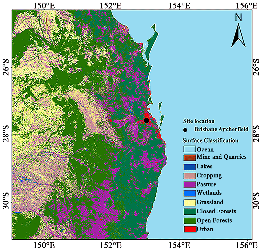
Figure 1The map of eastern Australia with land-cover types. The observation site is marked by a black dot.
2.2 Data
Several types of data have been used in this study, including land-cover-type data, Modern-Era Retrospective analysis for Research and Applications version 2 (MERRA-2) data, Moderate Resolution Imaging Spectroradiometer (MODIS) data, ground site observation data, the Fifth Version of European Centre for Medium-Range Weather Forecasts (ECMWF) ReAnalysis (ERA5) data, fire spot and FRP data and Global Data Assimilation System (GDAS) data. The detailed data information is described below one by one.
Land-cover-type data. The land-cover-type data of Australia are from the Dynamic Land Cover Dataset (DLCD) with Version 2.1 provided by Geoscience Australia. In this study, the DLCD land-cover-type data were used to reveal the surrounding landscape of Brisbane Archerfield. The spatial resolution of the data is 0.002∘ × 0.002∘, which is based on the annual mean of satellite observations from 2014 to 2015.
MERRA-2 data. MERRA-2 belongs to the global atmospheric reanalysis product managed by the National Aeronautics and Space Administration (NASA). It is produced by the Global Modeling and Assimilation Office (GMAO), and the assimilation system of Goddard Earth Observing System (GEOS-5) is used to ensure the quality of this dataset. At major ground sites over Australia, Yang et al. (2021) compared the monthly aerosol optical depth (AOD) product with Aerosol Robotic Network (AERONET) observations and found their root mean square errors (RMSEs) were all smaller than 0.05. Thus, MERRA-2 should be reliable to be used for the analysis of the large-scale spatial distribution of AOD in Australia. Yang et al. (2021) also denoted that the 2019 Australian mega fires were the strongest in January 2020. Correspondingly, we used the monthly AOD in January at 550 nm from 2002 to 2020 to check the AOD difference between the mega fire year and years with no mega fires. The spatial resolution of MERRA-2 AOD data is 0.625∘ × 1∘.
MODIS data. The MODIS instrument is performed on Aqua and Terra platforms. In this study, we used the MODIS cloud product which belongs to the dataset of MCD06COSP_M3_MODIS. The cloud information includes cloud optical depth (COD) and cloud fraction for all January months during the period from 2003 to 2020 with a monthly time resolution. The Brisbane Archerfield site is located at 153.008∘ E, 27.57∘ S. So we used COD and cloud fraction data whose space range and resolution are 152.5–153.5∘ E × 28.5–26.5∘ S and 1∘ × 1∘ respectively. This spatial range covers the whole Brisbane area and the normal encroaching distance of SLB, which is about tens of kilometres (Rajib and Heekwa, 2010; Shen et al., 2019). In this study, their spatial averages were calculated to represent the local COD and cloud fraction every January from 2003 to 2020. Also, we used the MODIS monthly AOD product for comparison with that of MERRA-2, which belongs to the dataset of MOD08_M3. The spatial resolution of MODIS AOD data is 1∘ × 1∘, and the time range is the same as that of MERRA-2.
Ground site observation data. The wind and air temperature observation data are from National Oceanic and Atmospheric Administration (NOAA) global observation network at the site of Brisbane Archerfield (153.008∘ E, 27.57∘ S). We used data in January from 2001 to 2020 in this study. The time resolution is every 3 h at 02:00, 05:00, 08:00, 11:00, 14:00, 17:00, 20:00 and 23:00 UTC on most days. The continuity of the observation data is ensured; there are observations on each day in January throughout the whole study period, with only one missing observation data on each day of a small fraction time (approximately 3.5 %). The wind information includes wind speed and wind direction. The air temperature is measured in Fahrenheit, and we have converted it into Celsius. The observation data were the main data used in this study to show the variations of both SLB and air temperature during the fire.
ERA5 data. The monthly mean U wind (zonal) speed and V wind (meridional) speed in January 2020 from the ERA5 were used in this study to reveal the background meteorological field so as to assess its effect on aerosol transport. The spatial resolution is 0.250∘ × 0.250∘ at pressure levels of 1000, 975, 950, 925, 900, 875, 850, 825, 800, 775, 750 and 700 hPa.
Fire spot and FRP data. Fire spot and FRP data are from the MODIS product (MCD14). This product can catch and locate the active fire hotspots based on thermal anomalies of 1 km pixel resolution (Giglio et al., 2016). The time resolution is daily, and we used the monthly averages for January from 2002 to 2020 to look into the fire situations over the years in detail.
GDAS data. The GDAS data were used to perform the back-trajectory analysis from the Hybrid Single-Particle Lagrangian Integrated Trajectory (HYSPLIT). The spatial resolution of GDAS data is 1∘ × 1∘ with daily time resolution. The levels of GDAS data chosen in this study to help to perform HYSPLIT analysis were 500 m and 3 km respectively. The time range set in this study was the whole of January 2020.
2.3 Methods
2.3.1 Extracting SLB signal
The verification of OE-SLB and extraction of SLB signals from original wind observation over monsoon areas were carried out through the method of the separation of the regional wind field (SRWF). The definition of OE-SLB, the details of SRWF method and the criterion for verification were detailed in our previous studies and are not repeated here (Shen et al., 2019; Shen and Zhao, 2020; Shen et al., 2021). Briefly speaking, SRWF calculates the vector difference between observed wind vector and daily average wind vector for each observation time. Then, the vector difference is considered to be the local wind. The criterion of OE-SLB requires that there are intersection sets among the range of SW, the range of LW and the range of hourly average of wind angle in a diurnal period (HAWADP). Also, the intersection set between the range of SW (LW) and the range of HAWADP only exists during daytime (night-time). Then the local wind can be thought as the SLB signal as long as the OE-SLB is verified at that site. Based on HAWADP and specific sea–land distribution, we further defined the prevailing time of sea wind (PTS) and prevailing time of land wind (PTL). Briefly speaking, during PTS (PTL) the local wind keeps blowing from sea (land), and the wind angle keeps rotating towards the direction of vast sea (inland). The HAWADP at Brisbane Archerfield is shown in Fig. 2. As shown, the HAWADP of local wind was close to sinusoid, which conformed to previous findings in other monsoon areas (Shen et al., 2021; Yan and Anthes, 1987). According to the sea–land distribution shown in Fig. 1, we first defined the ranges of SW and LW, and then the OE-SLB of Brisbane Archerfield was verified using these criteria. We further selected the PTS (PTL) based on the rules above.
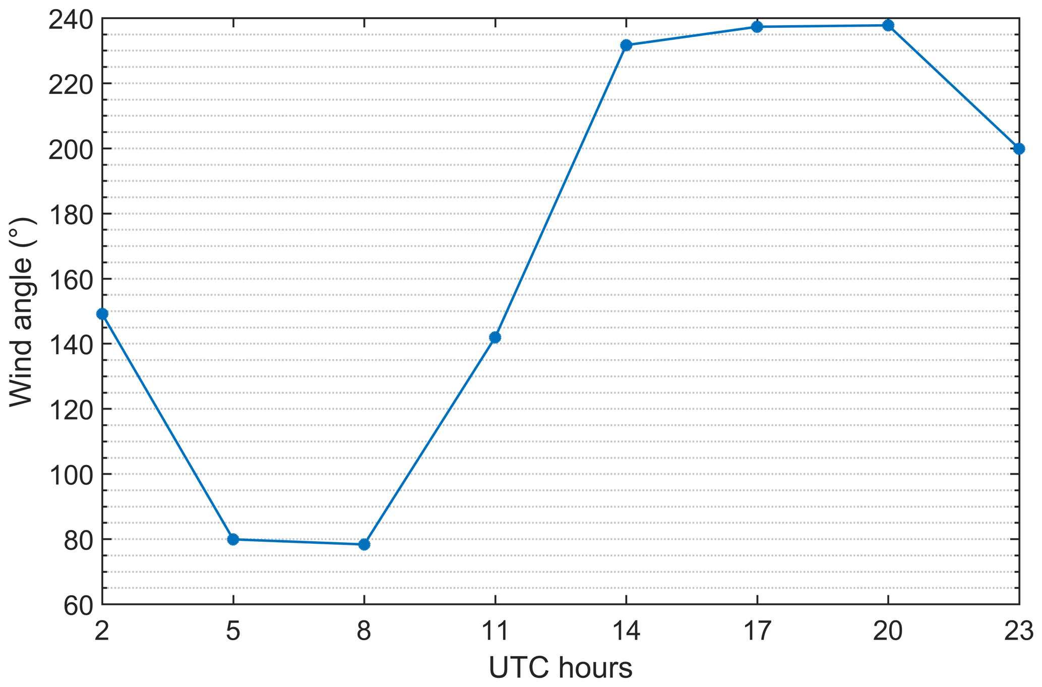
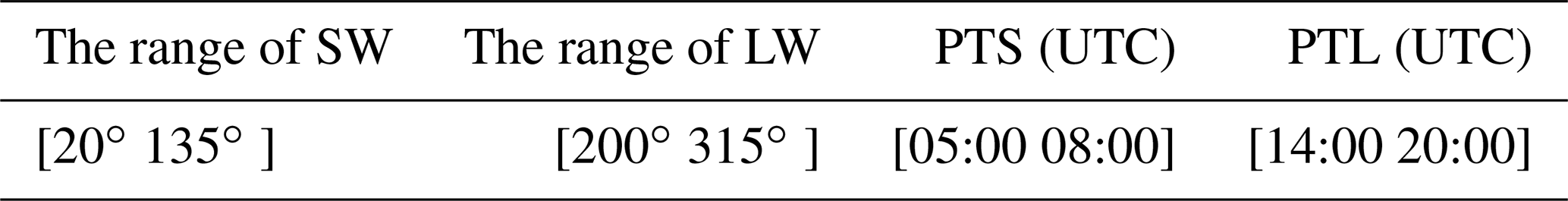
To make it clear, we summarize the range of SW, LW, PTS and PTL in Table 1. The ranges of SW and LW refer to specific sea–land distribution. Notably, there are few mountains within the ranges of SW and LW based on the accurate site location and detailed landscape nearby, which helps to exclude potential interruption from other small-scale circulations like mountain–valley wind. Note that the actual PTS (PTL) may be longer than what we defined here because the time resolution is 3 h instead of hourly in this study. As a result, we cannot know the exact threshold of time when the wind angle meets the criteria mentioned above. For instance, it is possible that the wind angle is within the range of SW before 05:00 UTC. However, it is still certain that the SW (LW) develops vigorously during 05:00–08:00 UTC (14:00–20:00 UTC) based on Fig. 2, which means that 05:00–08:00 UTC and 14:00–20:00 UTC are within the real PTS and PTL respectively, even if they are not the exact PTS or PTL. Thus, the PTS (PTL) defined in this study is reliable. The aim of defining PTS (PTL) is to find the time period when SW (LW) develops most vigorously so as to ensure further exclusion of winds from synoptic scales when trying to extract real SLB signals after applying the SRWF method (Shen and Zhao, 2020; Shen et al., 2021; Cuxart et al., 2014).
Table 1Summary of information for the verification of OE-SLB at Brisbane Archerfield.
2.3.2 Definition of the SLB day
The SLB day is the day when SLB circulation is most significant (Xue et al., 1995). To some extent, the number of SLB days reveals the activity level of SLB. Different criteria have been adopted when defining the SLB day. Here we referred to our previous study (Shen et al., 2019) to adopt the criteria based on the minimum times of successful detection of winds coming from the range of SW (LW) during PTS (PTL). Since the time interval between two adjacent observations is 3 h, which makes the number of total observation times less than the total hours during prevailing time, we modified the criteria slightly as follows: when the offshore land winds occur in the period of 14:00–20:00 UTC with a total occurrence time of no fewer than three times, and the onshore sea winds occur in the period of 05:00–08:00 UTC with a total occurrence time of no fewer than two times, the day is counted as a SLB day.
2.3.3 The calculation of monthly SW and LW speeds
After defining PTS, PTL and SLB day, we could finally calculate the monthly SW and LW speeds. First, we picked up SLB days in every January from 2001 to 2020. Second, we picked up local wind speed during PTS (PTL) on SLB days and calculated the monthly average of SW (LW) speed in every January from 2001 to 2020.
Based on GDAS data throughout the whole of January 2020, the back trajectories of the lower atmosphere at Brisbane Archerfield were simulated using the HYSPLIT model, which could help analyse the effect of background wind fields on aerosol transport at this site. The simulated levels at the site were 500 m and 3 km since the lower level of the atmosphere (500 m) was closer to fire spots, and there was also accumulated smoke at 3 km in the southeastern parts of Australia during the exact same month (Yang et al., 2021). The TrajStat module of Meteoinfo version 2.4.1 was also used to cluster the back trajectories based on the Euclidean distance method, whose details and source code can be found on its official website (http://meteothink.org/docs/trajstat/index.html, last access: 31 January 2021).
2.3.4 The calculation of monthly temperature during daytime and night-time
After defining the SLB day, PTS and PTL, we calculated the monthly mean temperature during daytime and night-time using the similar method as SW and LW speeds. First we selected the temperature on SLB days. Second, we calculated the monthly average of temperature during PTS (PTL) to represent monthly average temperature during daytime (night-time) in January. Actually, temperature during daytime (night-time) represents land temperature when SW (LW) prevails. In order to make it clear and concise, we call it temperature during PTS (PTL) or land temperature during daytime (night-time) in this study.
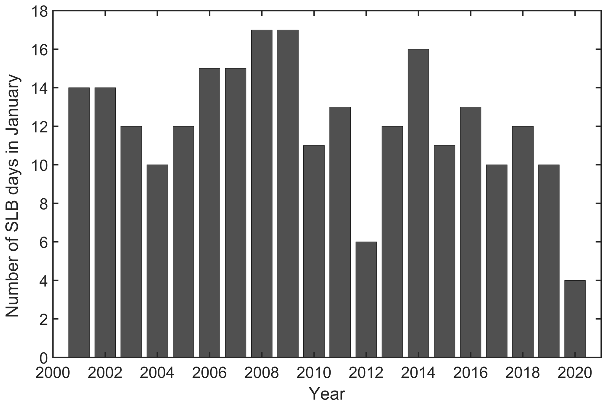
3.1 The variation of SLB day number
Figure 3 shows the SLB day number in January from 2001 to 2020. As shown, the SLB day number in January was normally larger than 10. Among these 20 years, there were 25 % of the years whose SLB days in January accounted for more than half of the month. Note that it does not necessarily mean that there is no SLB on days that are not SLB days. It is obvious that there was a slump in the number of SLB days in 2020. The total SLB day number dropped to only 4 during mega fires, accounting for only 33.33 % of the average SLB day number during the past 20 years. Also, the year 2012 witnessed a low SLB day number (6 d) in January. There are a lot of potential influencing factors for SLB frequency, such as the background wind field (Miller et al., 2013) and the interruption of other small-scale circulations (Kusaka et al., 2000). Among all the influencing factors, cloud is one of the most important because it has a significant effect on in situ solar radiation, which is the direct cause of TDLS. We will discuss this in the following sections.
3.2 The trends in SW and LW speeds and local air temperature
The monthly mean SW and LW speeds in January from 2001 to 2020 are shown in Fig. 4a. As can be seen, there were fluctuations in the trends of both SW and LW speeds. The SW speed was higher than LW speed, which conformed to many previous findings (Miller et al., 2013; Zhu et al., 2017). The averages were calculated as 3.70 m/s for SW speed and 2.86 m/s for LW speed, respectively. Figure 4b and c show the anomalies of both SW and LW speeds. In general, LW speed fluctuated more significantly than SW speed did. This is due to its lower level of kinetic energy which can make it more sensitive to any potential interruptions from the background meteorological field (Shen and Zhao, 2020). The negative anomalies of LW speed happened in 2001, 2004, 2008, 2010, 2011, 2015, 2016, 2017, 2018 and 2020. Different from other years, it is obvious that the negative anomaly in 2020 was higher than 0.6 m/s, which was beyond the multi-years' oscillation range. The anomaly accounted for 22.3 % of the multi-years' average LW speed. The negative anomalies of SW speed happened in 2004, 2008, 2009, 2010, 2011, 2013, 2014, 2015, 2017 and 2020 (Fig. 4c). For SW speed, the negative anomaly in 2020 was also obvious, but its value was still within the multi-year oscillation range. It was higher than 0.5 m/s, accounting for 14.8 % of the multi-years' average. It is interesting to find that there were obvious positive anomalies of both SW and LW speeds in 2003, whereas their absolute values were not the highest. Also, the SLB day number in 2003 was near the average. We will discuss this further, along with the aerosol emissions during that year, in the following sections.
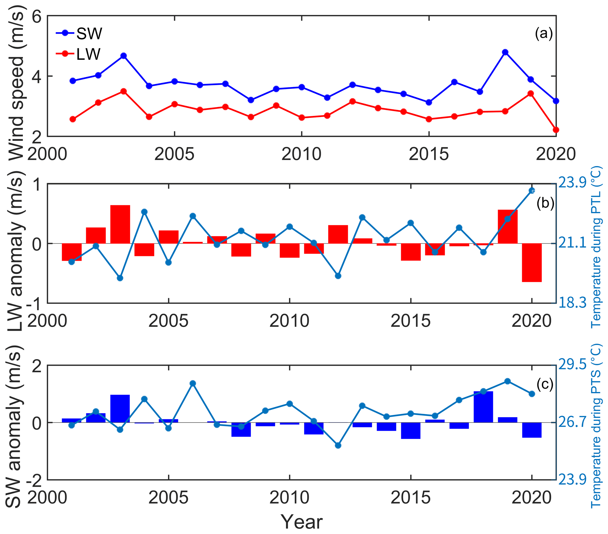
Figure 4The trends of SW and LW speeds (a), the LW speed anomaly and land temperature during night-time (b) and the SW speed anomaly and land temperature during daytime (c) based on their monthly average during January from 2001 to 2020.
It can be seen in Fig. 4b that there were also significant fluctuations in night-time land temperature over the years. There was a soar in land temperature during night-time in 2020 which approached nearly 24 ∘C. It was nearly 3 ∘C higher than the multi-years' average, exceeding the range of multi-years' oscillation. The fluctuation in land temperature during daytime was less significant than that during night-time. There was an obvious positive anomaly in 2020, indicating that the daytime land temperature was higher than that in normal years. Meanwhile, it was still within the range of multi-years' oscillation, though the positive anomaly was obvious. Fire spots have a heating effect on the nearby environment through either shortwave radiation of light from fires or heat conduction caused by a temperature gradient. It can be inferred that the mega wild fires in January 2020 contributed to the positive temperature anomalies during PTS (PTL) through the heating effect of fires, though they might not be the only cause. The heating effect during mega fires was more significant during night-time than during daytime, which is probably due to a colder background temperature field during night-time.
Basically, the decreased SW (LW) speed revealed that the TDLS during PTS (PTL) decreased. To be more specific, the temperature difference between the small regions where the upward stream and downward stream of SLB circulation lie became smaller during January 2020. Based on Fig. 4b and c, temperature during PTL seems to be generally negatively related to LW speed anomaly, while it is obvious that temperature during PTS does not show any corresponding relationship with SW anomaly.
In order to be more accurate, we carried out linear regression between temperature during PTL and LW anomaly and found that they had a negative linear relationship (p<0.02) with each other (Fig. 5). As the temperature increased by 10 ∘C, the LW speed anomaly decreased by 1.52 m/s. The correlation coefficient R was 0.52, which was at the medium level. However, considering the significance level as well as low level of sample number, it can be concluded that the LW speed is generally negatively correlated with night-time land temperature. Moreover, their R and significance level could be 0.69 and 0.0012 respectively if we excluded the only one abnormal point in 2019, which might be caused by some potential disturbances on coastal SST where the vertical stream of SLB lies. Considering all these, it can be concluded that the LW speed anomaly is generally negatively correlated with night-time land temperature. During night-time, the land is colder than the sea. As the land temperature increases, the TDLS decreases if the SST of the area where the upward stream of SLB lies remains relatively stable; the LW speed does too. Briefly, the good linear relationship reveals that the variation of temperature during PTL (night-time land temperature) could generally represent the variation of TDLS during PTL, while the daytime land temperature variation could not represent the TDLS variation during PTS. In our previous study, we also found through observation that the daily lowest temperature (DLT) was clearly negatively related to LW speed, while the SW speed was more related to in situ downwelling solar radiation rather than merely land temperature (Shen et al., 2021), which was similar to the findings here. It could be inferred that although the land temperature during daytime increased during mega fire events, TDLS was still narrowed during fire events. If we only consider the land temperature, the SW speed should have increased during fire events because SW circulation is formed due to warmer land and colder sea. Consequently, there should be other factors which could cause decreased TDLS during PTS, which is the direct cause of decreased SW speed. We would investigate this in the following sections.

Figure 5The relationship between LW anomaly and temperature during PTL based on their monthly average during January from 2001 to 2020.
3.3 The distribution and FRP of fire spots
Since the heating effect depends largely on the distance between the area heated and the heat centre, it is necessary to examine the distribution of fire spots in January over the years, which is shown in Fig. 6. It can be seen that fire spots are scattered all over the eastern part of Australia in January over the years. January is the middle of Australian summer, which is the season when wild fires happen most frequently (Yang et al., 2021). Apart from 2020, other years also witnessed considerable scattered fire spots all over the coastal and inland regions. It is obvious that there was an extreme fire centre in the southeastern corner of Australia with a great density of fire spots in January 2020. This was exactly the region where the 2019 Australian mega fires mainly happened. To be specific, it was the eastern corner of the state of Victoria and the southeastern corner of the state of New South Wales, which is in agreement with many reports in the media. There was also a great fire centre in the southeastern corner in 2003, although the scale was smaller than that in 2020. Considering the distribution of fire spots near the site, the density of fire spots nearby was not higher than in other years. Instead, there seems to be more fire spots nearby the site in 2003, 2005, 2006, 2010 and 2013 in the figure. If we restrained the nearby region to areas of smaller scales, the year 2003 and 2013 rather than 2020 would have the most nearby fire spots.
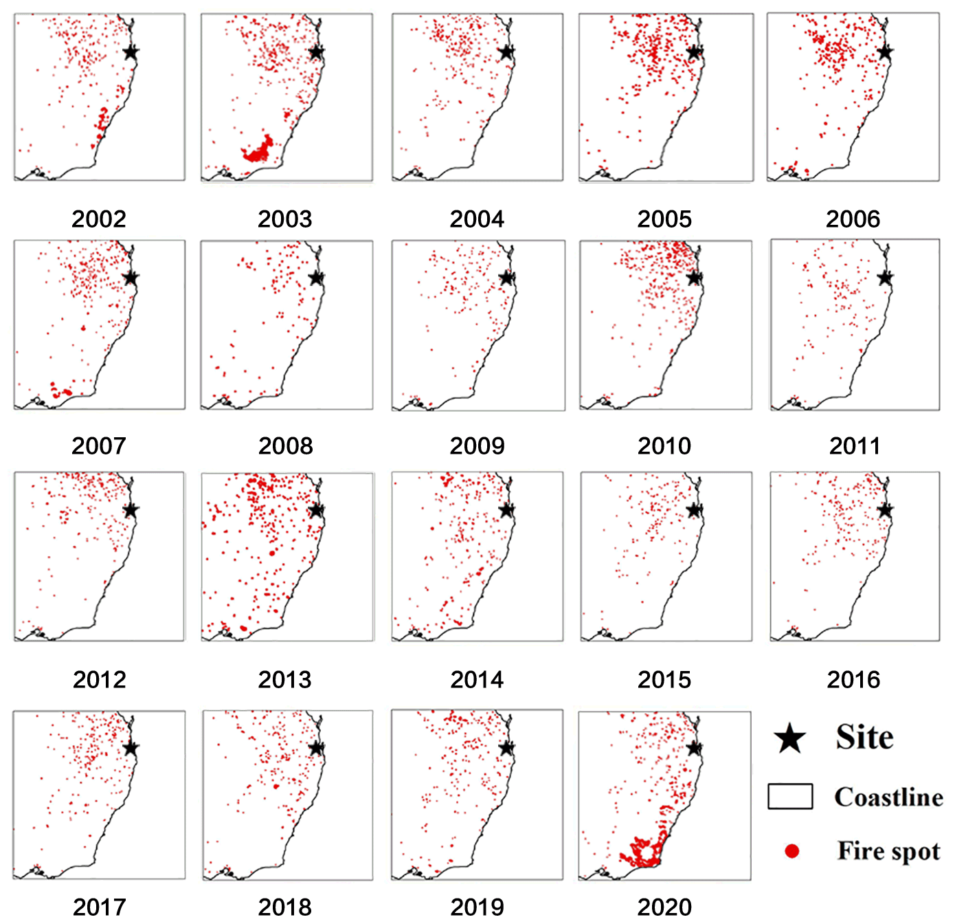
Figure 6The fire spot distribution in eastern Australia during January from 2002 to 2020.
There is another possibility that although the fire spots nearby the site were not more concentrated with great density in 2020 than in other years, the FRP of fire spots in 2020 was higher. This means that the fire was greater regardless of the ordinary density of spots, which could also result in more fire-induced aerosol emissions. So we further examined the FRP of fire spots in 2020 and those in other years. In order to make it comparable and verifiable, the time period of data chosen here was the same as that in Fig. 6. As shown in Fig. 7a, both the nearby and local fire spots in 2020 were mostly within the lowest FRP range, which was less than 235 MW. There were some sparse fire spots with greater FRP (235–863 MW) scattered all over the eastern part of Australia. The FRP of the fire centre was higher than the FRP of other fire spots; there were many fire spots with greater FRP which belonged to the range of 235–863 MW or 863–2194 MW. Figure 7b shows the FRP of all fire spots from 2002–2019. The FRP of nearby or local fire spots also had the lowest values. As the number of years increased, the density of fire spots with higher FRP (235–863 MW) increased significantly, most of which were located in inland areas of the Australian continent. This indicates that scattered wild fires with low or medium FRP are common in Australia, but concentrated mega fires are not so common. There were also some fire spots which belonged to the range of 235–863 MW or 863–2194 MW in 2003, yet the number was less, and the distribution areas were smaller. Based on Fig. 7, one important point we found is that there was no discrepancy between FRP of nearby or local fire spots in 2020 and that of nearby or local fire spots in other years. So the possibility mentioned above was discarded.
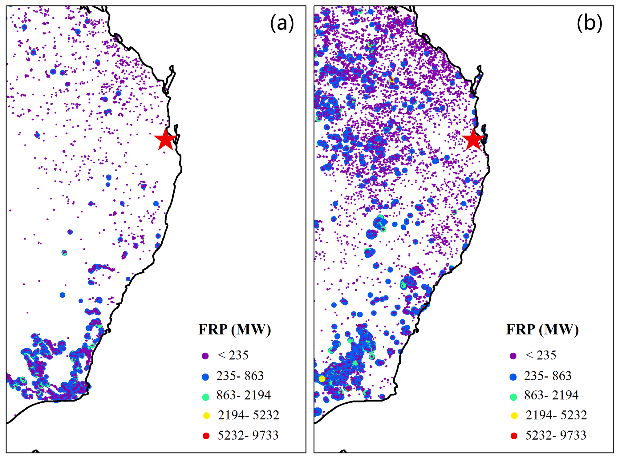
Figure 7The fire radiative power (FRP) of total fire spots in eastern Australia during January 2020 (a) and January from 2002 to 2019 (b).
Based on the analysis above, the nearby fire spot density and FRP in 2020 were both at the same level as in other years for local regions near the site. This implies that the heating effect of nearby fire spots did exist in 2020, contributing to the increase of land temperature to some extent (especially night-time land temperature), but it was not likely the major cause of the land temperature anomaly. Fluctuation in land temperature might be caused by combined mechanisms, including some other potential factors. In other words, the heating effect of fire spots does not necessarily correspond to the observed air temperature increase. For example, Fig. 4b and c show that there were negative land temperature anomalies in 2003, but actually this year witnessed a greater density of nearby or local fire spots. In a real situation, the scale of SLB is quite small. The fire spots might be quite a long distance away from the area where the vertical stream of SLB lies, as a result of which the heating effect is weak.
3.4 The spatial distribution of aerosols
Large fires have great aerosol emissions which affect the in situ solar radiation and then the radiation budget. Based on the basic physical mechanism of SLB formation, the observed decreased SW and LW speeds demonstrated the decreased TDLS. As mentioned above, the heating effect of nearby fire spots was weak and did not become more significant in 2020. So the more important factors bringing about the decrease of SW and LW speeds should be more closely related to TDLS rather than the land temperature only. The TDLS during SLB formation is highly related to the in situ downwelling solar radiation. As the shortwave radiation increases, the TDLS becomes larger due to the different heat capacities between land and sea. SW forms and prevails when TDLS is enough to drive this thermodynamic circulation. During night-time, the land–sea system is a “heater” for the upper atmosphere as the land and sea both give out heat and undergo energy loss in the form of longwave radiation. As the outgoing longwave radiation increases, the TDLS also becomes larger due to the different heat capacities between the land and sea. Then the LW forms in a similar way to SW.
Based on discussions above, in situ downwelling solar radiation is a crucial influencing factor of SW speed. Considering that aerosol is an important factor affecting in situ downwelling solar radiation, it is necessary for us to check the temporal and spatial variations of aerosols over the years. Figures 8 and 9 show the spatial distribution of AOD of total aerosols (TA-AOD) over the years using MERRA-2 and MODIS aerosol products, respectively. It shows that except for a little overestimation of AOD in the fire centre in 2020, the overall distribution and value of AOD revealed by MERRA-2 agreed well with those revealed by MODIS. Both MERRA-2 and MODIS show that there was a burst of aerosols in the fire centre during January 2003 and 2020, and the latter was much more severe. Especially for the site learned in this study, the difference of AODs between MERRA-2 (approximately 0.26) and MODIS (approximately 0.29) was very small. Thus, MERRA-2 agreed well with both MODIS and AERONET in terms of AOD during mega fires, and it has higher spatial resolution than MODIS. Considering all these aspects and the focus of the study, we used the MERRA-2 product in the analysis on local aerosol variations in the following sections. Figure 8 shows that the background level of TA-AOD was generally low in Australia over the years, implying that Australia was less polluted as a result of human activities. The TA-AOD in 2020 increased significantly compared with the average level. It can be seen that there was a maximum value centre in the southeast corner, which overlapped the region of the fire spots' centre (Fig. 6). The peripheral area of the maximum value centre was covered with isopleths, showing the characteristics of free diffusion of aerosols in the air. There was also a maximum value centre in 2003 whose scale was smaller, overlapping the smaller region of the fire centre in 2003. Based on findings from these three aspects, it can be concluded that the mega fire centre was the main source of the large amounts of aerosols around the site location. In general, the TA-AOD was about 240 % of the multi-years' average level at the site, while the TA-AOD in the fire centre was at a more astonishing level, accounting for more than 420 % of that at the local site of Brisbane. Aerosol could significantly affect the in situ downwelling solar radiation through direct radiative forcing. Turnock et al. (2015) calculated the relationship between AOD and surface solar radiation (SSR) and found that when the background value is low over the years, the SSR increases by 10 % as AOD varies from 0.32 to 0.16. In this study, the TA-AOD increased even more significantly (240 %), considering the low background value. Normally, when we talk about the radiative forcing of aerosols in the form of SSR difference, it means the instantaneous radiative forcing. However, the formation of SLB is the result of different levels of radiation accumulations between the land and sea. So the effect of aerosols on the total in situ downwelling solar radiation can further accumulate in the process of SLB formation and results in even more significant impacts on the change of surface temperature.
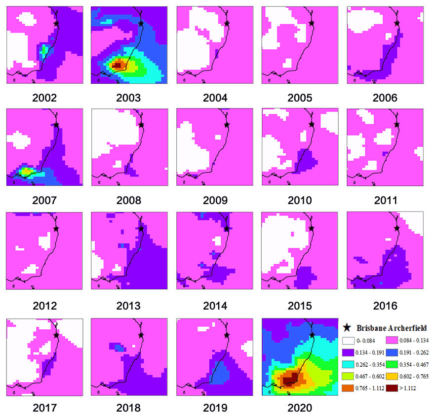
Figure 8The spatial distribution of aerosol optical depth (AOD) of total aerosols in eastern Australia during January from 2002 to 2020 using the Modern-Era Retrospective analysis for Research and Applications version 2 (MERRA-2) AOD product.
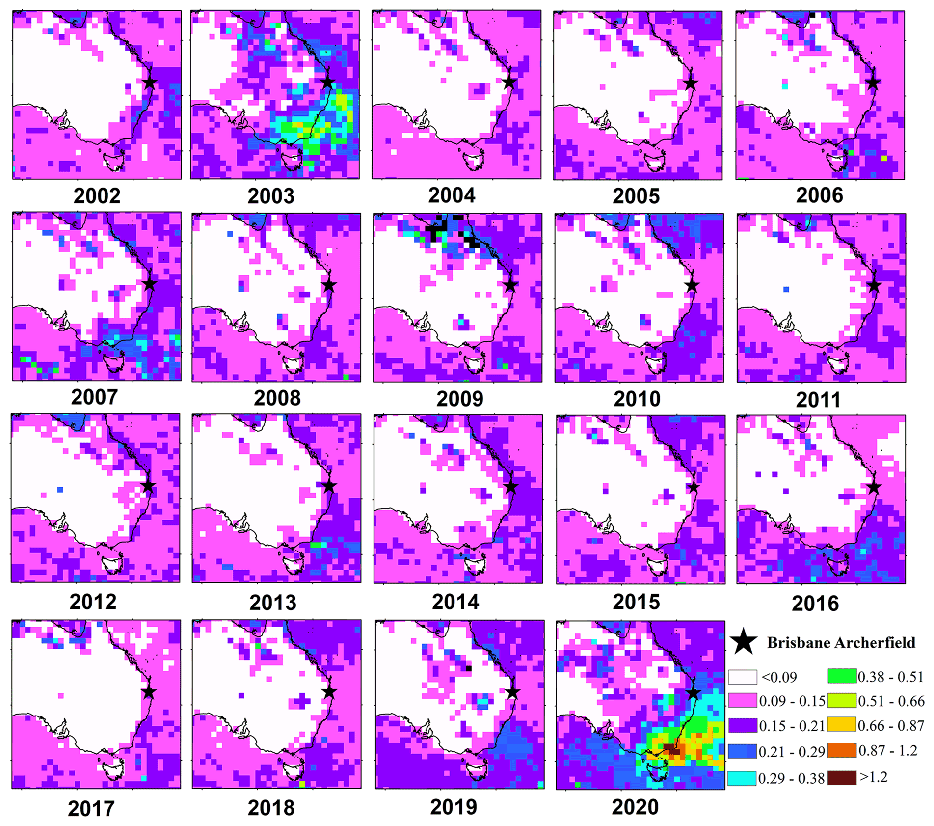
Figure 9The spatial distribution of aerosol optical depth (AOD) of total aerosols in eastern Australia during January from 2002 to 2020 using the Moderate Resolution Imaging Spectroradiometer (MODIS) AOD product.
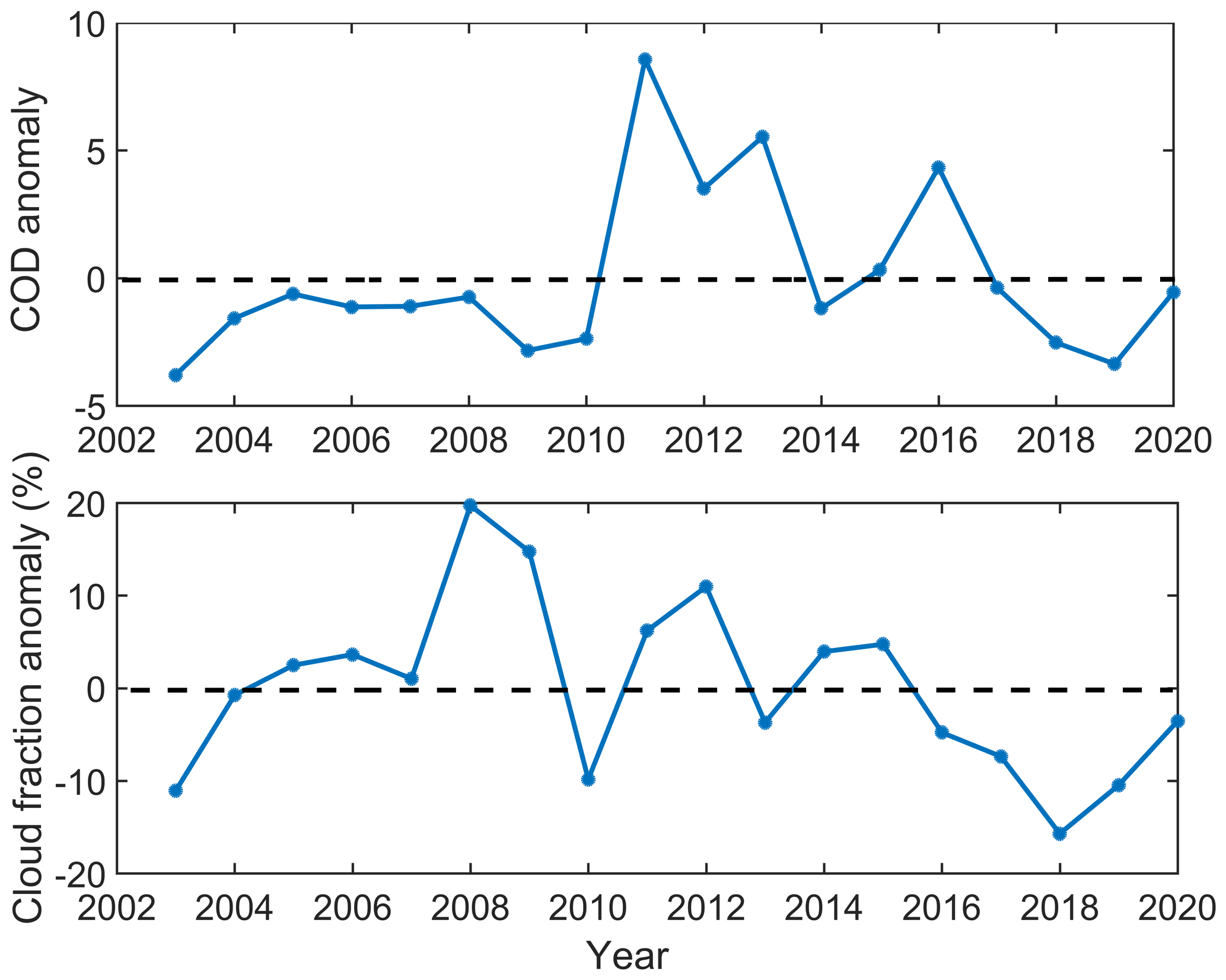
Figure 10The monthly cloud optical depth (COD) anomaly and cloud fraction anomaly at Brisbane Archerfield during January from 2003 to 2020.
Apart from aerosols, clouds could play an even more important role in the radiation budget. The COD and cloud fraction anomaly at this site are shown in Fig. 10. The time range was from 2003 to 2020 due to data availability. It can be seen that both the cloud fraction and COD in 2003 were at an obvious low level, while both the cloud fraction and COD in 2020 showed a tiny negative anomaly. Based on the spatial distribution of TA-AOD, both 2003 and 2020 witnessed a soar in TA-AOD at the site, while TA-AOD increased more significantly in 2020. Figure 3 shows that there was a slump in SLB number in 2020 but not in 2003, while Fig. 4 shows that there were positive anomalies of both SW and LW speeds in 2003. Many previous studies on SLB have pointed out that a high level of in situ downwelling solar radiation is favourable for SLB formation and SLB speed increase (Shen and Zhao, 2020; Shen et al., 2021b; Miller et al., 2013). Our previous study in a monsoon climate region also showed that there was a positive linear relationship between in situ downwelling solar radiation and SW speed (Shen and Zhao, 2020). As we know, the in situ downwelling solar radiation is determined by both cloud and aerosols through their combined “umbrella effect”. The finding shown in Figs. 3 and 4 could be explained by the radiative cooling effects of aerosols and clouds. Although there was a positive anomaly of TA-AOD in 2003, the COD and cloud fraction were less than the average, offsetting the aerosols' negative radiative forcing effect. In situ downwelling solar radiation of the regional sea–land system was still ensured so that the SLB happened with a normal frequency (Fig. 3) and with an even larger speed (Fig. 4). The in situ downwelling solar radiation in January 2020 should be lower than the average, considering the tiny negative anomaly in both COD and cloud fraction and the significant increase in TA-AOD. The increased radiative forcing effect of TA-AOD was accumulated during the formation of SW. In conclusion, during daytime, the negative radiative forcing effect of total aerosols was the determinant factor to weaken the in situ downwelling solar radiation, resulting in lower level of TDLS and then decreased SW speed.
Mega fire events are significant in the way that they emit large amounts of carbonaceous aerosols, which include OC and BC. The OC is a very good scatter to solar radiation. Thus, among all the aerosols, OC could be an important contributor to the weakened TDLS during SW formation. Figure 11 shows the spatial distribution of OC over the years. The spatial distribution of OC was also similar to the fire spot distribution, which further confirmed that the source of great aerosol emissions was the mega fire centre. There were extreme value centres in the fire centre in both 2003 and 2020. The same as what we found earlier, it can be seen that the large values spread further in 2020 than 2003, indicating that the fire events were more severe in 2020 than in 2003. Similarly, the background value of OC at the site was low on average. The specific value of organic carbon AOD (OC-AOD) at the Brisbane site in 2020 was about 630 % of the multi-years' average, which was even higher than that of total aerosol. This is easy to understand because the fire centre is also covered with plants and trees, and their combustion can result in significant amounts of carbonaceous aerosols. Zhang et al. (2017) estimated the radiative forcing of OC globally using the BCC_AGCM2.0_CUACE/Aero model, which showed that Brisbane was within the large value area, with high levels of negative radiative forcing at the top of atmosphere. They also attributed this to biomass combustion. Thus, both total aerosol and OC made great contributions to the SW speed decrease by decreasing in situ downwelling solar radiation in January 2020.
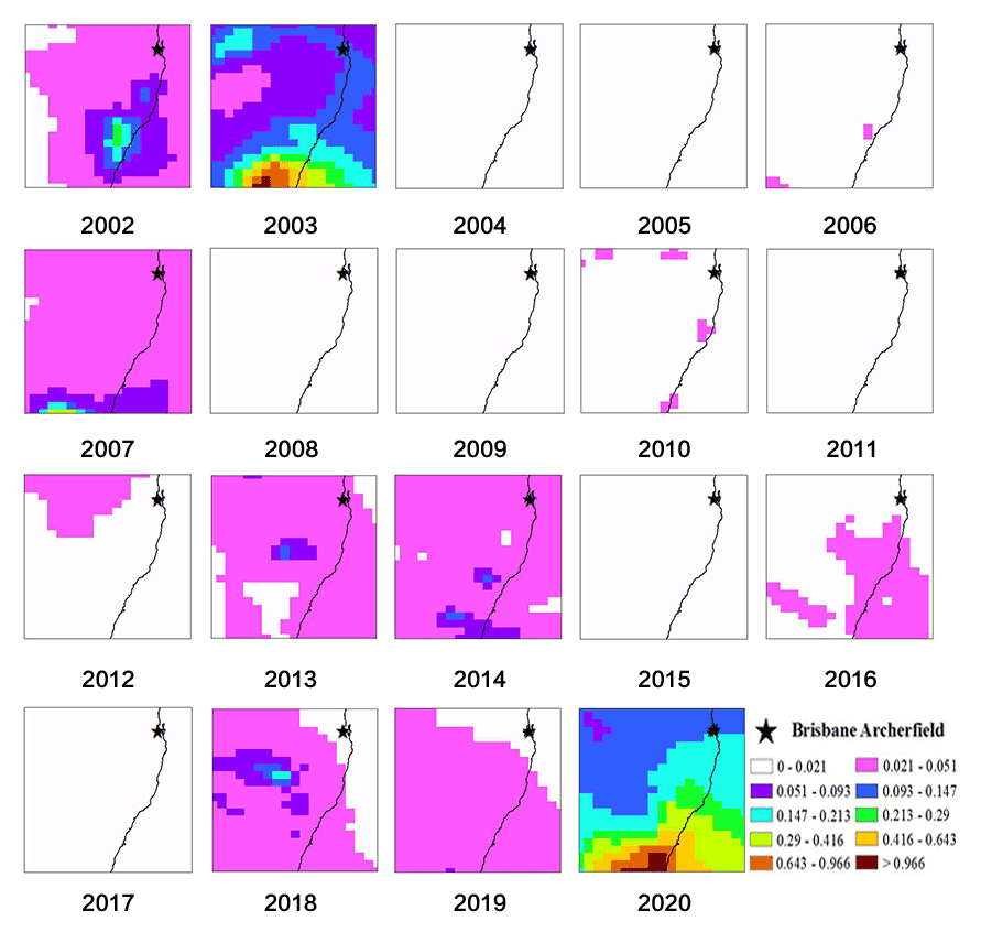
Figure 11The spatial distribution of aerosol optical depth (AOD) of organic carbon (OC) in eastern Australia during January from 2002 to 2020.

Figure 12The spatial distribution of aerosol optical depth (AOD) of black carbon (BC) in eastern Australia during January from 2002 to 2020.
The result above is analysed based on the impacts of aerosols on solar radiation. However there is almost no shortwave radiation during night-time. Then one question pops up: why was the slump of LW speed more significant? This indicated that the TDLS was significantly weakened at night in January 2020. While the heating effect of fire spots on night-time land temperature did exist, which was more significant than that during daytime, it was not likely the main cause of weakened TDLS based on FRP and fire spot distribution analysis. We next investigated the spatial distribution of BC over the years in Fig. 12. It shows that the black carbon AOD (BC-AOD) at the site was about 425 % of the multi-years' average level, with the extreme value centre overlapping the area of that of fire spots' density. Similar to the distribution of TA-AOD and OC-AOD, the peripheral areas of the maximum value centre are covered with isopleths, showing the characteristics of free diffusion. BC is well known as a kind of absorbing aerosol, which is reported to have a wider range of absorbing band than greenhouse gases, which can absorb broadband radiation from visible light to infrared wavelength (Zhang et al., 2017). During the daytime, it can absorb solar radiation, longwave radiation from the warmer land and shortwave radiation from local fires. During night-time, it has a warming effect on both the atmosphere and Earth's surface through longwave radiation. As a result, it has a warming effect on the Earth–atmosphere system, including the surface of the regional land–sea system, so there is a soaring of temperature, shown in Fig. 4b. The soaring BC during the mega fire heated the local atmosphere, which was like adding a heater in the air. The heater then gave out downward longwave radiation to the regional land–sea system. Just like the Sun during daytime, this could trigger a SW circulation anomaly, weakening LW circulation. Considering the BC burst during mega fires, there is nothing weird about its dominant role in the local land temperature increase during night-time. The mechanism proposed above can be summarized as follows. During night-time, the formation of LW originates from the process of heat release from both land and sea. As they both lose heat at different paces due to different heat capacities, the TDLS is enlarged. During the mega fires, the upper atmosphere of the regional land–sea system is heated, so that the vertical temperature gradient is weakened, which is unfavourable for heat release from both sea and land surfaces. As a result, the TDLS is significantly weakened.
Another potential contributing accelerator is CO2, which is also the product of fires due to the combustion of plants and trees. CO2 is a kind of greenhouse gas which is likely to be engaged in the same mechanism as BC to reduce TDLS during night-time, except that CO2 cannot affect the downwelling solar radiation. Details about this are not repeated again. However we should note that the effect of CO2 is based on theoretical analysis rather than observational verification due to the lack of accurate observation data. Both BC and CO2's warming effects increase TDLS during daytime, which partially offsets the strong negative radiative forcing effect of total aerosols, but their combined warming effect is more significant during night-time than during daytime. That is most likely the reason (at least partially) that SW speed had a negative anomaly but was less significant than LW speed.
What we discussed above are all factors whose influences were restrained to a small scale. Although SLB is a small-scale system, it can still be affected by the variations of signals on a large scale, since the local temperature is affected by both regional forcing and the variation of the large-scale background temperature field. In our previous study, we weighed their contributions qualitatively (Shen et al., 2019). In this study, we simply discuss the potential effect of the change in large-scale SST. Hirsch and Koren (2021) emphasized the effect of record-breaking aerosol emission from this mega fire on the cooling of the oceanic areas. On a large scale, its average radiative forcing on sea surface was −1.0 ± 0.6 W/m2. The temperature decrease of large-scale sea surface could have negative forcing on the SST at a regional scale, though the specific temperature variation of the sea surface where the SLB vertical stream lies might not be the same.
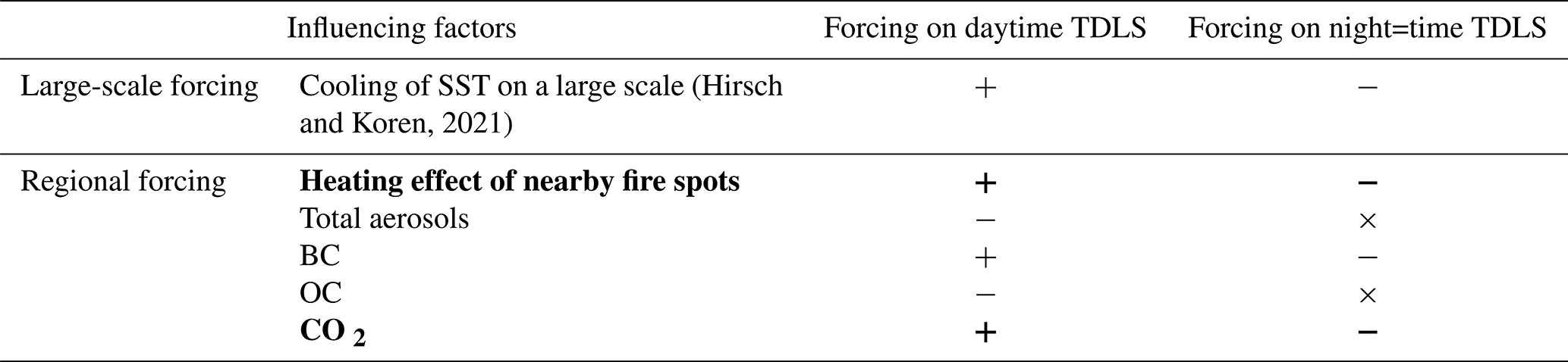
We summarized all the influencing factors of TDLS at both regional and large scales in Table 2. Among all these factors, aerosols, BC, OC and CO2 had direct forcing on TDLS by changing the solar radiation reaching the regional sea–land system. In contrast, the heating effect of fire spots and large-scale SST signal had forcing on land temperature and regional SST respectively, thus further having different forcing effects on TDLS during daytime and night-time. During the 2019 Australian mega fires, TDLS during daytime and night-time both decreased under their combined forcing effects, which could be inferred from the anomalies of SLB speed. Clearly, the directions of all forcing effects of different factors were the same during night-time. That was why LW speed decreased much more significantly than SW speed did. The negative radiative forcing effect of total aerosols was the determinant cause for TDLS decrease during daytime, which could only be partially offset by other factors.
Table 2Summary of the effect of different factors on TDLS. Factors marked in bold represent that they are either a weak factor or a potential factor derived from theoretical analysis but not verified by observation.
3.5 Source of aerosols
3.5.1 Fire centre's emission
As indicated earlier, the year 2020 did not have advantages over other years in terms of local and nearby fire spot density and FRP in January. Note that certain land-cover types could also increase the aerosol emissions. For example, if there was more combustible land cover such as forests or plants, the fires could emit more carbonaceous aerosols in the form of smoke. Considering this possibility, we further checked the latest version of land cover in Australia online (http://maps.elie.ucl.ac.be/CCI/viewer/index.php, last access: 1 April 2021). It was updated to 2019, which overlapped with the starting time of the 2019 Australian mega fires. It showed that the areas and density of flora near the site were stable over the years, implying that the soaring in local aerosols during mega fires was not likely caused by the change of land cover either.
As Figs. 6, 8, 11 and 12 show, the distributions of fire spots, TA-AOD, BC-AOD and OC-AOD were quite similar to each other. In the fire centre, both the density and FRP of fire spots were much higher in January 2020 than in January of other years, which are all based on distribution characteristics at a large scale. In order to show the fire situation at the fire centre more accurately, we magnified the FRP map to restrain the areas to merely the fire centre, which is shown in Fig. 13. As shown, the fire spot density was quite high in this region, especially along coastal areas. Compared with other areas, the fire centre had much more fire spots with higher FRP. The spots with FRP from 235 to 864 MW were evenly distributed in all fire areas, surrounded by low FRP spots with high density. There were quite a few spots with even higher FRP ranging from 864 to 2194 MW, which could not be found in other peripheral areas (Fig. 7a). In some areas at the fire centre, we could even find fire spots with FRP ranging from 2194 to 5232 MW. All these distribution characteristics of fire spots suggest the possibility of large amounts of aerosols including smoke being emitted into the atmosphere, after which a great concentration gradient in the horizontal direction is formed between the fire centre and farther areas. Based on basic chemistry law, irreversible free diffusion would happen in this process. As the concentration gap increases, the diffusion efficiency also increases. The distribution of contour lines in Figs. 8, 11 and 12 also shows the characteristics of free diffusion. A similar mechanism works out for the spatial distribution of CO2 during the fire events.

Figure 13The detailed distribution of fire spots and their FRP in the fire centre during January 2020.
3.5.2 Analysis on the background wind field
Apart from free diffusion, wind is crucial for pollution transport including aerosols (Walcek, 2002). Also, wind is a key factor of the near-surface CO2 distribution (Cao et al., 2017). Zhang et al. (2017) confirmed that BC could be transported over long distances in mid-latitude areas. The transport distance of OC was even longer than that of BC. It is necessary for us to look into the background wind field in order to know the likely aerosol transport from the fire centre to the site. Yang et al. (2021) retrieved the average status of the vertical distribution of various aerosols in southeastern Australia during the 2019 Australian mega fires and found most of them accumulated under 3 km, which is about 700 hPa. Figure 14 shows the monthly average background wind field based on wind information at pressure levels from 1000 to 700 hPa in January 2020. The red cross symbols represent the fire spots in this figure. The average background wind field clearly revealed the existence of the Southern Hemisphere's westerlies and a subtropical high. The fire centre was approximately located at the intersection of the northern boundary of the westerlies and the southwestern boundary of the subtropical high. Since January is the middle month of Australian summer, the subtropical high developed quite vigorously, some of which stretched into the eastern part of the Australian continent. It covered the areas where most fire spots were located. At a large scale, this caused quite a hot and dry background meteorological field, which was favourable for the development and persistence of wild fires. Based on the average status of wind fields at different pressure levels, the subtropical high and westerlies together formed a background wind field blowing from the site to the fire centre, which was unfavourable for the aerosol transport from the fire centre to the site. However, we should notice that this figure merely describes the monthly average status; it ignores the status of wind flows at a more accurate fine timescale. In other words, it is still possible that aerosols from the fire centre were transported to the site within some short periods in January 2020, contributing to the significant positive anomalies in AODs shown in Figs. 8, 9, 11 and 12. Based on the specific dates of SLB days during mega fires identified in the previous section, which were 4, 14, 20 and 28 January respectively, we divided January 2020 into five short time periods by excluding the identified SLB days. These five short time periods were all named the “no-SLB period”. We did the backward trajectory analysis during each no-SLB period to see if the aerosols from the fire centre were transported to the site with the help of the background wind field, thus further confirming this period to be a no-SLB period through all the mechanisms mentioned above. It is easy to understand that the near-surface concentration of aerosol should be at a high level in general, not only because it was near the fire spots, but also because it was within the boundary layer. Considering these aspects, the backward trajectory analysis was carried out at 500 m over the site. Figure 15a–e show the wind backward trajectories at this site during the five no-SLB periods respectively. During the no-SLB periods of (a), (c), (d) and (e), the winds mainly came from the southern Pacific to the east of Australia continent, which could not transport aerosols from the fire centre. There were winds coming from the fire centre merely during period (b). The northern edge of the wind flow beam was quite near the fire centre, and then it went further towards the northeastern direction in the southern Pacific. When it reached the general position of the subtropical high, it turned back to the direction of northwest before finally reaching the site. The high-pressure gradient between the centre and edge of the subtropical high was opposite to its moving direction, which might be the cause of its abrupt turning. Although the southwestern edge of the subtropical high itself had wind flows whose directions were away from the Australian continent at a monthly average (Fig. 14), the wind flows from the northern edge of the Southern Hemisphere's westerlies could still move along its southwestern edge as soon as they intersected with each other if a smaller timescale and a single level were considered (Fig. 15b). Figure 15f showed the contributions of the main backward trajectories based on the whole month's statistics. The main backward trajectories were calculated after the clustering of all trajectories, whose number was based on a certain mathematical method like the calculation of total spatial variation (TSV). More details of this clustering method and contribution calculation can be found on the official website of this software (http://meteothink.org/docs/trajstat/cluster_cal.html, last access: 31 March 2021). It can be seen that the wind flows which could potentially bring aerosols from the fire centre still had a little contribution, which accounted for 9.32 % (2.87 % + 6.45 %). In contrast, winds coming from the Pacific to the east and northeast of the Australian continent dominated the wind field at the site, whose contributions were 25.09 % and 54.12 % respectively. Thus, the contribution of wind transport to increasing local aerosols should be limited, which was only found during one period with a time length less than 10 d in January 2020. From the perspective of multi-layers of the atmosphere (0–3 km), the multi-layers of the background wind fields as a whole did not contribute to the aerosol and CO2 transport from the fire centre to the site. Therefore, the soaring of aerosols including BC and OC at the site should mainly be caused by the combined effect of combustion in the fire centre and great free diffusion caused by a significant concentration gradient, with a likely relatively weak contribution of the wind transport.
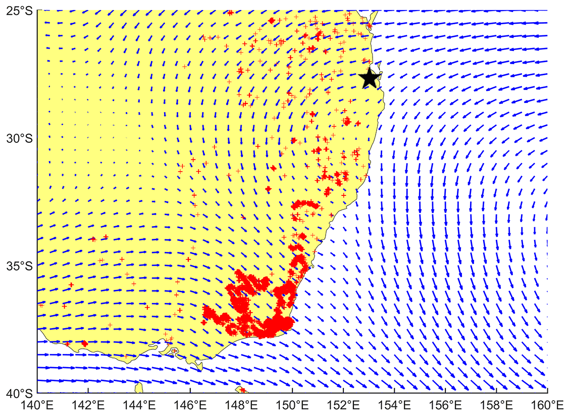
Figure 14Monthly average background wind field based on wind information at pressure levels from 100 to 700 hPa in January 2020. The red crosses present fire spots, and the black star represents the site location.
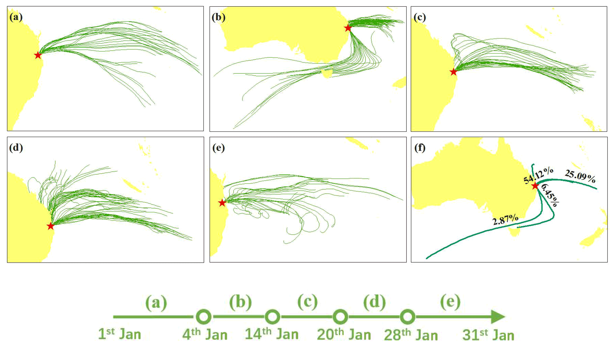
Figure 15The site's wind backward trajectories at 500 m during January 2020. The wind backward trajectories during the first no-SLB period from 1 to 3 January (a), the wind backward trajectories during the second no-SLB period from 5 to 13 January (b), the wind backward trajectories during the third no-SLB period from 15 to 19 January (c), the wind backward trajectories during the fourth no-SLB period from 21 to 27 January (d), the wind backward trajectories during the fifth no-SLB period from 29 to 31 January (e) and the contribution of the four main wind clusters based on the wind backward trajectories during the whole month of January 2020 (f).
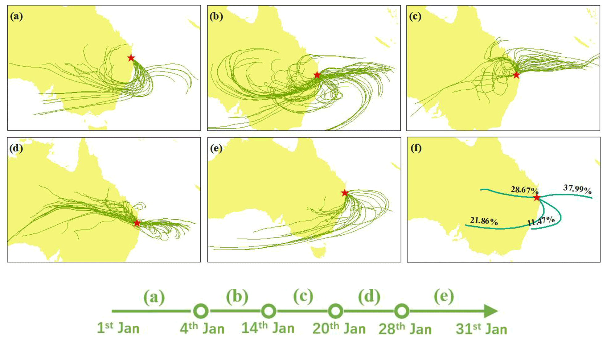
Figure 16The site's wind backward trajectories at 3 km during January 2020. The wind backward trajectories during the first no-SLB period from 1 to 3 January (a), the wind backward trajectories during the second no-SLB period from 5 to 13 January (b), the wind backward trajectories during the third no-SLB period from 15 to 19 January (c), the wind backward trajectories during the fourth no-SLB period from 21 to 27 January (d), the wind backward trajectories during the fifth no-SLB period from 29 to 31 January (e) and the contribution of the four main wind clusters based on the wind backward trajectories during the whole month of January 2020 (f).
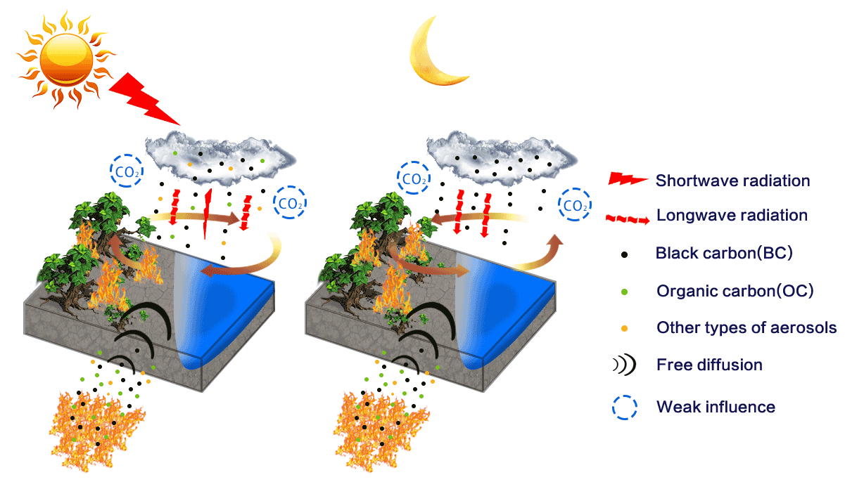
Figure 17The summary of mechanisms containing influencing factors of local SLB during daytime and night-time. The larger fire cluster represents the centre of mega fires with a higher concentration of all types of aerosols. During the Australian mega fires, aerosols were transported to the local site by means of free diffusion, which was caused by the great concentration gap of aerosols between the fire centre and the local site. The width of arrows of “shortwave radiation” represents the magnitude of shortwave radiation.
Most aerosols are generally within the atmospheric boundary layer under normal conditions, while this might be different under the situation during mega fires considering the boost of vertical movement due to the great heat release from fires and astonishing amounts of aerosol emissions. Smoke, as a kind of unique aerosol emission produced in great amounts during fire events, could be essential to SW and LW speed anomalies due to its absorptive radiative properties, making it particularly valuable to examine its transport individually. Yang et al. (2021) analysed the vertical distribution of smoke on southeastern parts of Australia, which included the fire centre and the site, and found that the smoke accumulated at 3 km generally. Considering this aspect, we also did the backward trajectory analysis at 3 km, whose time division was the same as that at 500 m. The results are shown in Fig. 16. As shown, the wind flow scattered more evenly at 3 km than at 500 m. There were more wind flows coming from the southwestern direction of the site. This is probably due to the fact that the magnitude and stretching area of westerlies are larger in the upper atmosphere than in layers closer to the surface. During period (a), (b) and (e), there were clusters of wind flows coming from the fire centre or near the fire centre, which could bring aerosols to the site. Specifically, there were wind flows penetrating the fire centre directly during period (a) and (e), while the wind flows during period (b) are only adjacent to the north edge of fire centre. Since the period (b) was the longest among all no-SLB periods, it did not necessarily mean that the wind's aerosol transport effect during this period was less than that during other periods, although the wind flows were not directly from the fire centre. Their moving paths were similar to those of wind flows in Fig. 15b, which all showed an abrupt turn on the Pacific to the southeast of the site. This is probably because the Southern Hemisphere's subtropical high developed to be quite strong during the middle of summer, making the pressure gradient exist both at 500 m and 3 km (Fig. 14). Figure 16f shows the contribution of wind flows on monthly average, whose clustering number was also 4. There were four main directions of wind flows, whose contributions were 28.67 %, 21.86 %, 11.47 % and 37.99 % respectively. For clarity, we define these four main wind flows as wind flow clusters. The wind flow clusters with contributions of 21.86 % and 11.47 % were generally adjacent to the north edge of the fire centre, which contained a contribution of wind flows from the fire centre. Due to the clustering limitation of Meteoinfo, we could not extract the specific contributions of wind flows blowing directly from the fire centre from the total contributions of wind flow clusters (21.86 % and 11.47 %). But based on analysis from shorter time periods, their contributions were larger than those at 500 m because there were more no-SLB periods with wind flows blowing from the fire centre.
In this study, the SLB day number, SLB speed, daytime temperature and night-time temperature at Brisbane Archerfield in January were calculated from 2001 to 2020 using observation data from automatic meteorological stations. We have taken three steps in total to exclude the interference of winds from synoptic-scale systems in order to extract the real SLB signals. First, we used a SRWF method to verify the OE-SLB and then extracted the SLB signal from original observation. Second, we defined the SLB days as when the whole SLB circulation is most significant and integrated. Finally, we used SLB signals during PTS (PTL) on SLB days to calculate the monthly average of SW (LW) speed. In the corresponding months over the years, regional cloud fraction, COD, fire spot and FRP distribution in Australia were revealed using the MODIS product. Comparison with MODIS and site observations confirmed the good quality of the MERRA-2 product to reveal the variation of aerosols during mega fires. Consequently, aerosols' distributions in eastern Australia were revealed in the form of AOD using the MERRA-2 product, including that of total aerosols, OC and BC. Furthermore, the background wind field and backward wind trajectory were analysed using the ERA5 product and HYSPLIT respectively. The main findings of this study are as follows.
-
There was a significant slump in SLB day number (33.3 % of the average level) and LW speed (decreased by 22.3 % of the average level) at the site. While SW speed also decreased by 14.8 % of the average level, it was not significant.
-
There was a burst of aerosols at the site, with TA-AOD, BC-AOD and OC-AOD being approximately 240 %, 425 % and 630 % of the multi-years' averages. TDLS is a direct cause of SLB, while other factors influence SLB through their effects on TDLS. The variation of night-time land temperature could generally represent the variation of TDLS during night-time, while TDLS during daytime could not be simply represented by daytime land temperature. Specifically, the significant aerosol burst was mainly responsible for the decrease of SW speed. The burst of BC at the site, as well as the large-scale SST decrease during mega fires, was mainly responsible for the slump of LW speed. CO2 emitted by nearby fire spots or transmitted from the fire centre was a potential and weak factor of the slump of LW speed. The heating effect of nearby fires on TDLS was weak during both daytime and night-time.
-
Emissions from the fire centre were mainly responsible for the local positive aerosol anomaly during mega fires. On average, the background wind fields from the near surface to 3 km were unfavourable for aerosol and CO2 transport. But there was likely aerosol and CO2 transport through a large-scale wind field at single levels during shorter periods within January 2020. Specifically, the wind flow transport at 3 km was stronger than that at 500 m, which was particularly important for smoke transport since the smoke from fires gathered at the same level. In general, free diffusion due to a large concentration gradient was mainly responsible for aerosol transport and the potential CO2 transport, while the effect of background wind field played a secondary role.
In order to make the influencing factors of SLB clear and concise, we summarized their potential mechanisms in a local sea–land system (Fig. 17). During the daytime, a negative anomaly of SW speed was found at the site in January 2020 when the Australian mega fires were most intense. The local cloud fraction and COD were almost on an average level, while there were significantly more aerosols during mega fires, which mainly came from the fire centre by free diffusion. They significantly weakened the in situ downwelling solar radiation, thus further narrowing the TDLS, which was the direct cause of SW speed decrease. BC and CO2 heated the atmosphere and warmed the earth–atmosphere system by longwave radiation from the heated atmosphere. The warming effect of BC and CO2, the decrease of SST at a large scale and the weak heating effect of nearby fire spots partially offset the effect of aerosols on narrowing TDLS, making the negative SW speed anomaly not exceed the multi-years' oscillation range. During night-time, the heating effect of nearby fire spots was still weak but more significant than that during daytime. The warming effect of BC and CO2 was like adding a heater in the atmosphere, which triggered a SW circulation anomaly, thus resulting in a slump in LW speed. The decrease of SST at a large scale further boosted the decrease of LW speed. The slumps in both SLB speed and SLB day number could help to accumulate the local aerosols (Shen and Zhao, 2020), which further catalysed the physical processes mentioned in the mechanism and finally formed a positive feedback mechanism under a scenario of mega fires.
Essentially, a narrowed TDLS was the direct cause of SLB speed decrease, which was affected by various factors in the form of either shortwave radiation or longwave radiation. It not only weakened the SLB speed, but also brought about a slump in the SLB day number. The in situ radiation, including both longwave and shortwave radiation reaching the ground, has a direct impact on the TDLS considering the basic physical mechanism of SLB formation. Note that the specific weather condition, cloud fraction, COD and the type of clouds and aerosols could all affect the in situ radiation. Apart from in situ radiation, the heat release in urban areas, heat waves, heating effect of nearby heat sources, large-scale signals of SST and land surface temperature variation could all affect TDLS by changing either the local land temperature or SST. The large-scale signals of temperature variations could be caused by either natural variability or human variability. Normally, SLB forms when the TDLS is obvious and the background wind field is mild. So the condition of a large-scale wind field such as a monsoon is also an important influencing factor of SLB. Apart from the slump in both SLB day number and LW speed during mega fire events, there were smaller fluctuations in both of their trends, which need to be studied further in future.
The Dynamic Land Cover Dataset (DLCD) can be accessed thorough Geoscience Australia (http://www.ga.gov.au/scientific-topics/earth-obs/accessing-satellite-imagery/landcover, Lymburner et al., 2015). MERRA-2 Reanalysis data can be accessed through the NASA Global Modeling and Assimilation Office (https://gmao.gsfc.nasa.gov/reanalysis/MERRA-2/, Global Modeling and Assimilation Office (GMAO), 2015). MODIS observation data can be accessed through the Earthdata centre managed by NOAA (https://earthdata.nasa.gov/search?q=MCD06, MODIS Atmosphere Science Team, 2015; http://earthdata.nasa.gov/search?q=MOD08, Hubanks et al., 2015). GDAS data used in HYSPLIT data are accessible through the NOAA READY website (http://www.ready.noaa.gov, NOAA, 2016). Fire spot and FRP data can be accessed from the MODIS MCD14 product managed by NOAA (https://earthdata.nasa.gov/search?q=MCD14, The Land, Atmosphere Near real-time Capability for EOS MODIS (LANCEMODIS) Team, 2015). The wind and temperature observation data from the NOAA global observation network can be accessed on NOAA's official website (http://www1.ncdc.noaa.gov/pub/data/noaa/, Baldwin et al., 2020). The ERA5 data can be accessed through the official website of the Copernicus project (https://climate.copernicus.eu/climate-reanalysis, Hersbach et al., 2021).
CZ and LS developed the ideas and designed the study. LS, XY, YY and PZ contributed to collection and analyses of data. LS and XY performed the analysis and prepared the manuscript. CZ supervised and modified the manuscript. All authors made substantial contributions to this work.
The contact author has declared that neither they nor their co-authors have any competing interests.
Publisher's note: Copernicus Publications remains neutral with regard to jurisdictional claims in published maps and institutional affiliations.
This work was supported by the Ministry of Science and Technology of China National Key Research and Development Program (2019YFA0606803), the National Natural Science Foundation of China (41925022), the State Key Laboratory of Earth Surface Processes and Resources Ecology and the Fundamental Research Funds for the Central Universities.
This research has been supported by the National Key Research and Development Program of China (grant no. 2019YFA0606803) and the National Outstanding Youth Science Fund Project of the National Natural Science Foundation of China (grant no. 41925022).
This paper was edited by Jianping Huang and reviewed by two anonymous referees.
Albrecht, B. A.: Aerosols, Cloud Microphysics, and Fractional Cloudiness, Science, 245, 1227–1230, https://doi.org/10.1126/science.245.4923.1227, 1989.
Baldwin, R., Wright, V., Anders, D. D., Brinegar, D., Lott, N., Jones, P., Smith, F., and Boreman, B.: The FCC Integrated Surface Hourly Database, A New Resource of Global Climate Data [data set], Data center of NOAA, available at: http://www1.ncdc.noaa.gov/pub/data/noaa/ (last access: 31 March 2021), 2020.
Cao, L. Z., Chen, X., Zhang, C., Kurban, A., Yuan, X. L., Pan, T., and Maeyer, P.: The temporal and spatial distributions of the near-surface CO2 concentrations in central Asia and analysis of their controlling factors, Atmosphere, 8, 1–14, https://doi.org/10.3390/atmos8050085, 2017.
Charlson, R. J., Schwartz, S. E., Hales, J. M., Cess, R. D., Coakley, J. A., Hansen, J. E., and Hofmann, D. J.: Climate forcing by anthropogenic aerosols, Science, 255, 423–430, 1992.
Chuang, C. C., Penner, J. E., Prospero, J. M., Grant, K. E., Rau, G. H., and Kawamoto, K.: Cloud susceptibility and the first aerosol indirect forcing: Sensitivity to black carbon and aerosol concentrations, J. Geophys. Res.-Atmos., 107, 4564, https://doi.org/10.1029/2000JD000215, 2002.
Cuxart, J., Jiménez, M. A., Prtenjak, M. T., and Grisogono, B.: Study of a sea-breeze case through momentum, temperature, and turbulence budgets, J. Appl. Meteorol. Climatol., 53, 2589–2609, 2014.
Garrett, T. J. and Zhao, C.: Increased Arctic cloud longwave emissivity associated with pollution from mid-latitudes, Nature, 440, 787–789, https://doi.org/10.1038/nature04636, 2006.
Giglio, L., Schroeder, W., and Justice, C. O.: The collection 6 MODIS active fire detection algorithm and fire products, Remote Sens. Environ., 178, 31–41, https://doi.org/10.1016/j.rse.2016.02.054, 2016.
Global Modeling and Assimilation Office (GMAO): MERRA-2 tavgM_2d_aer_Nx: 2d, Monthly mean, Time-averaged, Single-Level, Assimilation, Aerosol Diagnostics V5.12.4, Greenbelt, MD, USA, Goddard Earth Sciences Data and Information Services Center (GES DISC) [data set], https://doi.org/10.5067/FH9A0MLJPC7N, 2015.
Grandey, B. S., Lee, H.-H., and Wang, C.: Radiative effects of interannually varying vs. interannually invariant aerosol emissions from fires, Atmos. Chem. Phys., 16, 14495–14513, https://doi.org/10.5194/acp-16-14495-2016, 2016.
Han, W., Li, Z., Wu, F., Zhang, Y., Guo, J., Su, T., Cribb, M., Fan, J., Chen, T., Wei, J., and Lee, S.-S.: The mechanisms and seasonal differences of the impact of aerosols on daytime surface urban heat island effect, Atmos. Chem. Phys., 20, 6479–6493, https://doi.org/10.5194/acp-20-6479-2020, 2020.
Hersbach, H., Bell, B., Berrisford, P., Biavati, G., Horányi, A., Muñoz Sabater, J., Nicolas, J., Peubey, C., Radu, R., Rozum, I., Schepers, D., Simmons, A., Soci, C., Dee, D., and Thépaut, J.-N.: ERA5 monthly averaged data on single levels from 1979 to present, Copernicus Climate Change Service (C3S) Climate Data Store (CDS) [data set], available at: https://climate.copernicus.eu/climate-reanalysis (last access: 31 March 2021), 2019.
Hirsch, E. and Koren, I.: Record-breaking aerosol levels explained by smoke injection into the stratosphere, Science, 371, 1269–1274, https://doi.org/10.1126/science.abe1415, 2021.
Hubanks, P., Platnick, S., King, M., and Ridgway, B.: MODIS Atmosphere L3 Monthly Product. NASA MODIS Adaptive Processing System, Goddard Space Flight Center [data set], USA, https://doi.org/10.5067/MODIS/MOD08_M3.061, 2015.
IPCC: Intergovernmental Panel on Climate Change, Climate Change 2013: The Physical Science Basis, Contribution of Working Group I to the Fifth Assessment Report of the Intergovernmental Panel on Climate Change, Cambridge Univ. Press, Cambridge, UK, and New York, 1535 pp., 2013.
Jacobson, M. Z.: Strong radiative heating due to the mixing state of black carbon in atmospheric aerosols, Nature, 409, 695–697, 2001.
Jacobson, M. Z.: Effects of biomass burning on climate, accounting for heat and moisture fluxes, black and brown carbon, and cloud absorption effects, J. Geophys. Res.-Atmos., 119, 8980–9002, https://doi.org/10.1002/2014jd021861, 2014.
Jia, S. Q., Jing, J. L., Ju, E. D., and Chi, W. B.: Discussions on the temperature and pressure fields in a mega forest fire zone, J. Nort. Fore. Uni., 15, 226–232, https://doi.org/10.13759/j.cnki.dlxb.1987.s4.028, 1987.
Kloss, C., Berthet, G., Sellitto, P., Ploeger, F., Bucci, S., Khaykin, S., Jégou, F., Taha, G., Thomason, L. W., Barret, B., Le Flochmoen, E., von Hobe, M., Bossolasco, A., Bègue, N., and Legras, B.: Transport of the 2017 Canadian wildfire plume to the tropics via the Asian monsoon circulation, Atmos. Chem. Phys., 19, 13547–13567, https://doi.org/10.5194/acp-19-13547-2019, 2019.
Kusaka, H., Kimura, F., Hirakuchi, H., and Mizutori, M.: The effects of land-use alteration on the sea breeze and daytime heat island in the Tokyo metropolitan area, J. Meteorol. Soc. Jpn., 78, 405–420, https://doi.org/10.2151/jmsj1965.78.4_405, 2000.
Li, J. W., Yang, L. Q., Li, X. W., and Zheng, H. R.: Visualization of local wind field based forest-fire's forecast modeling for transportation planning, Multimed. Tools. Appl., 1, 1–15, https://doi.org/10.1007/s11042-016-3357-7, 2016.
Luhar, A. K., Mitchell, R. M., Meyer, C. P., Qin, Y., Campbell, S., Gras, J. L., and Parry, D.: Biomass burning emissions over northern Australia constrained by aerosol measurements: II–Model validation, and impacts on air quality and radiative forcing, Atmos. Environ., 42, 1647–1664, https://doi.org/10.1016/j.atmosenv.2007.12.040, 2008.
Lymburner, L., Tan, P., McIntyre, A., Thankappan, M., and Sixsmith, J.: Dynamic Land Cover Dataset Version 2.1. Geoscience Australia, Canberra, available at: http://pid.geoscience.gov.au/dataset/ga/83868 (last access: 31 January 2021), 2015.
Ma, Y., Gao, R. Z., and Miao, S. G.: Impacts of urbanization on summer-time SLB circulation in Qingdao, Acta. Sci. Circumst., 33, 1690–1696, https://doi.org/10.13671/j.hjkxxb.2013.06.030, 2013.
Mallet, M. D., Desservettaz, M. J., Miljevic, B., Milic, A., Ristovski, Z. D., Alroe, J., Cravigan, L. T., Jayaratne, E. R., Paton-Walsh, C., Griffith, D. W. T., Wilson, S. R., Kettlewell, G., van der Schoot, M. V., Selleck, P., Reisen, F., Lawson, S. J., Ward, J., Harnwell, J., Cheng, M., Gillett, R. W., Molloy, S. B., Howard, D., Nelson, P. F., Morrison, A. L., Edwards, G. C., Williams, A. G., Chambers, S. D., Werczynski, S., Williams, L. R., Winton, V. H. L., Atkinson, B., Wang, X., and Keywood, M. D.: Biomass burning emissions in north Australia during the early dry season: an overview of the 2014 SAFIRED campaign, Atmos. Chem. Phys., 17, 13681–13697, https://doi.org/10.5194/acp-17-13681-2017, 2017.
McCoy, D. T. and Hartmann, D. L.: Observations of a substantial cloud-aerosol indirect effectduring the 2014–2015 Bárðarbunga-Veiðivötnssure eruption in Iceland, Geophys. Res. Lett., 42, 10409–10414, https://doi.org/10.1002/2015GL067070, 2015.
Meyer, C. P., Luhar, A. K., and Mitchell, R. M.: Biomass burning emissions over northern Australia constrained by aerosol measurements: I – Modelling the distribution of hourly emissions, Atmos. Environ., 42, 1629–1646, https://doi.org/10.1016/j.atmosenv.2007.10.089, 2008.
Miller, S. T. K., Keim, B. D., Talbot, R. W., and Mao, H.: Sea breeze: Structure, forecasting, and impacts, Rev. Geophys., 41, 1011, https://doi.org/10.1029/2003RG000124, 2013.
Mitchell, R. M., O'Brien, D. M., and Campbell, S. K.: Characteristics and radiative impact of the aerosol generated by the Canberra firestorm of January 2003, J. Geophys. Res.-Atmos., 111, D02204, https://doi.org/10.1029/2005jd006304, 2006.
Mitchell, R. M., Forgan, B. W., Campbell, S. K., and Qin, Y.: The climatology of Australian tropical aerosol: Evidence for regional correlation, Geophys. Res. Lett., 40, 2384–2389, https://doi.org/10.1002/grl.50403, 2013.
MODIS Atmosphere Science Team: MODIS Cloud Properties Level 3 Monthly Product, NASA MODIS Adaptive Processing System, Goddard Space Flight Center [data set], USA, https://doi.org/10.5067/MODIS/MCD06COSP_M3_MODIS.061, 2015.
Nai, F. B., Zhao, L. N., and Wu, J. R.: Impacts of sea-land and mountain-valley circulations on the air pollution in Beijing-Tianjin-Hebei: a case study, Environ. Pollut., 234, 429–438, https://doi.org/10.1016/j.envpol.2017.11.066, 2018.
NOAA: GDAS – Daily Tar Files (1∘ by 1∘), NCEI's NOAA National Operational Model Archive and Distribution System (NOMADS) [data set], available at: ftp://ftp.arl.noaa.gov/pub/archives/gdas1 (last access: 31 March 2021), 2016.
Ohneiser, K., Ansmann, A., Baars, H., Seifert, P., Barja, B., Jimenez, C., Radenz, M., Teisseire, A., Floutsi, A., Haarig, M., Foth, A., Chudnovsky, A., Engelmann, R., Zamorano, F., Bühl, J., and Wandinger, U.: Smoke of extreme Australian bushfires observed in the stratosphere over Punta Arenas, Chile, in January 2020: optical thickness, lidar ratios, and depolarization ratios at 355 and 532 nm, Atmos. Chem. Phys., 20, 8003–8015, https://doi.org/10.5194/acp-20-8003-2020, 2020.
Portin, H., Mielonen, T., Leskinen, A., Arola, A., Pärjälä, E., Romakkaniemi, S., Laaksonen, A., Lehtinen, K. E. J., and Komppula, M.: Biomass burning aerosols observed in Eastern Finland during the Russian wildfires in summer 2010 e Part 1: In-situ aerosol characterization, Atmos. Environ., 47, 269–278, http:// https://doi.org/10.1016/j.atmosenv.2011.10.067, 2012.
Rajib, P. and Heekwa, L.: Estimation of the effective zone of sea/land breeze in a coastal area, Atmos. Pollut. Res., 2, 106–115, https://doi.org/10.5094/APR.2011.013, 2010.
Ramana, M. V., Ramanathan, V., Feng, Y., Yoon, S. C., Kim, S. W., Carmichael, G. R., and Schauer, J. J.: Warming influenced by the ratio of black carbon to sulphate and the black-carbon source, Nat. Geosci., 1, 542–545, https://doi.org/10.1038/NGEO918, 2010.
Sarker, A., Saraswat, R. S., Chandrasekar, A.: Numerical study of the effects of urban heat island on the characteristic features of the sea breeze circulation, P. Indian As.-Eng. Sci., 107, 127–137, 1998.
Shen, L. X. and Zhao, C. F.: Dominance of Shortwave Radiative Heating in the Sea-Land Breeze Amplitude and its Impacts on Atmospheric Visibility in Tokyo, Japan, J. Geophys. Res.-Atmos., 125, 1–19, https://doi.org/10.1029/2019jd031541, 2020.
Shen, L. X., Zhao, C. F., Ma, Z. S., Li, Z. Q., Li, J. P., and Wang, K. C.: Observed decrease of summer sea-land breeze in Shanghai from 1994 to 2014 and its association with urbanization, Atmos. Res., 227, 198–209, https://doi.org/10.1016/j.atmosres.2019.05.007, 2019.
Shen, L. X., Zhao, C. F., and Yang, X. C.: Insight Into the Seasonal Variations of the Sea-Land Breeze in Los Angeles With Respect to the Effects of Solar Radiation and Climate Type, J. Geophys. Res.-Atmos., 126, 1–21, https://doi.org/10.1029/2019jd033197, 2021a.
Shen, L. X., Zhao, C. F., and Yang, X. C.: Climate-Driven Characteristics of Sea-Land Breezes Over the Globe, Geophys. Res. Lett., 48, 1–10, https://doi.org/10.1029/2020GL092308, 2021b.
Sun, R. Y., Krueger, S. K., Jenkins, M. A., Zulauf, M. A., and Charney, J. J.: The importance of fire–atmosphere coupling and boundary-layer turbulence to wildfire spread, Int. J. Wildland Fire., 18, 50–60, https://doi.org/10.1071/WF07072, 2009.
The Land, Atmosphere Near real-time Capability for EOS MODIS (LANCEMODIS) Team: MODIS/Aqua Terra Thermal Anomalies/Fire locations 1 km FIRMS V006 NRT (Vector data), NASA MODIS Adaptive Processing System, Goddard Space Flight Center [data set], USA, https://doi.org/10.5067/FIRMS/MODIS/MCD14DL.NRT.006, 2015.
Torres, O., Jethva, H., Ahn, C., Jaross, G., and Loyola, D. G.: TROPOMI aerosol products: evaluation and observations of synoptic-scale carbonaceous aerosol plumes during 2018–2020, Atmos. Meas. Tech., 13, 6789–6806, https://doi.org/10.5194/amt-13-6789-2020, 2020.
Turnock, S. T., Spracklen, D. V., Carslaw, K. S., Mann, G. W., Woodhouse, M. T., Forster, P. M., Haywood, J., Johnson, C. E., Dalvi, M., Bellouin, N., and Sanchez-Lorenzo, A.: Modelled and observed changes in aerosols and surface solar radiation over Europe between 1960 and 2009, Atmos. Chem. Phys., 15, 9477–9500, https://doi.org/10.5194/acp-15-9477-2015, 2015.
van der Werf, G. R., Randerson, J. T., Giglio, L., Collatz, G. J., Kasibhatla, P. S., and Arellano Jr., A. F.: Interannual variability in global biomass burning emissions from 1997 to 2004, Atmos. Chem. Phys., 6, 3423–3441, https://doi.org/10.5194/acp-6-3423-2006, 2006.
Vermote, E., Ellicott, E., Dubovik, O., Lapyonok, T., Chin, M., Giglio, L., and Roberts, G. J.: An approach to estimate global biomass burning emissions of organic and black carbon from MODIS fire radiative power, J. Geophys. Res.-Atmos., 114, D18205, https://doi.org/10.1029/2008jd011188, 2009.
Walcek, C. J.: Effects of wind shear on pollution dispersion, Atmos. Environ., 36, 511–517, https://doi.org/10.1016/s1352-2310(01)00383-1, 2002.
Wang, Y., Jiang, J. H., and Su, H.: Atmospheric responses to the redistribution of anthropogenic aerosols, J. Geophys. Res.-Atmos., 120, 9625-9641, https://doi.org/10.1002/2015JD023665, 2015.
Xue, D. Q., Zheng, Q. L., and Qian, X. Z.: Features of sea-land circulation with its influence over Shandong Peninsula, J. Nanjing Inst. Meteorol., 18, 293–299, https://doi.org/10.13878/j.cnki.dqkxxb.1995.02.021, 1995.
Yan, H. and Anthes, R. A.: The effect of latitude on the sea breeze, Mon. Weather Rev., 115, 936–956, 1987.
Yang, X., Zhao, C. F., Zhou, L., Wang, Y., and Liu, X.: Distinct impact of different types of aerosols on surface solar radiation in China, J. Geophys. Res. Atmos., 121, 6459-6471, https://doi.org/10.1002/2016JD024938, 2016.
Yang, X., Zhao, C., Yang, Y., Yan, X., and Fan, H.: Statistical aerosol properties associated with fire events from 2002 to 2019 and a case analysis in 2019 over Australia, Atmos. Chem. Phys., 21, 3833–3853, https://doi.org/10.5194/acp-21-3833-2021, 2021.
Zhang, H., Wang, Z. L., and Zhao, S. Y.: Atmospheric aerosols and their climatological effect, China Meteorological Press, Beijing, China, ISBN: 978-7-5029-6676-8, 2017.
Zhao, C. and Garrett, T. J.: Effects of Arctic haze on surface cloud radiative forcing, Geophys. Res. Lett., 42, 557–564, https://doi.org/10.1002/2014gl062015, 2015.
Zhao, C., Lin, Y., Wu, F., Wang, Y., Li, Z., Rosenfeld, D., and Wang, Y.: Enlarging rainfall area of tropical cyclones by atmospheric aerosols, Geophys. Res. Lett., 45, 8604–8611, https://doi.org/10.1029/2018GL079427, 2018.
Zhao, C. F., Yang, Y. K., Fan, H., Huang, J. P., Fu, Y. F., Zhang, X. Y., Kang, S. C., Cong, Z. Y., Husi, L., and Menenti, M.: Aerosol characteristics and impacts on weather and climate over Tibetan Plateau, Nat. Sci. Rev., 7, 492–495, https://doi.org/10.1093/nsr/nwz184, 2020.
Zhu, L., Meng, Z., Zhang, F., and Markowski, P. M.: The influence of sea- and land-breeze circulations on the diurnal variability in precipitation over a tropical island, Atmos. Chem. Phys., 17, 13213–13232, https://doi.org/10.5194/acp-17-13213-2017, 2017.