the Creative Commons Attribution 4.0 License.
the Creative Commons Attribution 4.0 License.
 | 29 Mar 2022
Impact of biomass burning and stratospheric intrusions in the remote South Pacific Ocean troposphere
Nikos Daskalakis
Laura Gallardo
Maria Kanakidou
Johann Rasmus Nüß
Camilo Menares
Roberto Rondanelli
Anne M. Thompson
Mihalis Vrekoussis
The ozone mixing ratio spatiotemporal variability in the pristine South Pacific Ocean is studied, for the first time, using 21-year-long ozone (O3) records from the entire southern tropical and subtropical Pacific between 1994 and 2014. The analysis considered regional O3 vertical observations from ozonesondes, surface carbon monoxide (CO) observations from flasks, and three-dimensional chemistry-transport model simulations of the global troposphere. Two 21-year-long numerical simulations, with and without biomass burning emissions, were performed to disentangle the importance of biomass burning relative to stratospheric intrusions for ambient ozone levels in the region. Tagged tracers of O3 from the stratosphere and CO from various biomass burning regions have been used to track the impact of these different regions on the southern tropical Pacific O3 and CO levels. Patterns have been analyzed based on atmospheric dynamics variability.
Considering the interannual variability in the observations, the model can capture the observed ozone gradients in the troposphere with a positive bias of 7.5 % in the upper troposphere/lower stratosphere (UTLS) as well as near the surface. Remarkably, even the most pristine region of the global ocean is affected by distant biomass burning emissions by convective outflow through the mid and high troposphere and subsequent subsidence over the pristine oceanic region. Therefore, the biomass burning contribution to tropospheric CO levels maximizes in the UTLS. The Southeast Asian open fires have been identified as the major contributing source to CO from biomass burning in the tropical South Pacific, contributing on average for the study period about 8.5 and 13 ppbv of CO at Rapa Nui and Samoa, respectively, at an altitude of around 12 km during the burning season in the spring of the Southern Hemisphere. South America is the second-most important biomass burning source region that influences the study area. Its impact maximizes in the lower troposphere (6.5 ppbv for Rapa Nui and 3.8 ppbv for Samoa). All biomass burning sources contribute about 15–23 ppbv of CO at Rapa Nui and Samoa and account for about 25 % of the total CO in the entire troposphere of the tropical and subtropical South Pacific. This impact is also seen on tropospheric O3, to which biomass burning O3 precursor emissions contribute only a few ppbv during the burning period, while the stratosphere–troposphere exchange is the most important source of O3 for the mid troposphere of the South Pacific Ocean, contributing about 15–20 ppbv in the subtropics.
- Article
(8772 KB) - Full-text XML
-
Supplement
(549 KB) - BibTeX
- EndNote


Ozone (O3) is one of the major and most abundant oxidants in the Earth's atmosphere and a driver of tropospheric chemistry (Monks et al., 2015). Due to its oxidative power, O3 is also toxic for ecosystems and affects human health (Fleming et al., 2018; Jerrett et al., 2009; Mills et al., 2018; Pöschl and Shiraiwa, 2015). Tropospheric O3 is itself a greenhouse gas, capturing part of the Earth's outgoing longwave radiation, thus warming the atmosphere (Bowman et al., 2013; Lacis et al., 1990) and contributing about 25 % to the greenhouse gas forcing due to human activities (Monks et al., 2009; Myhre et al., 2013). The radiative forcing (RF) of O3 has been calculated based on the Climate Model Intercomparison Project phase 6 (CMIP6) simulations to be 0.28±0.17 W m−2 for the period 1850–2000 (Checa-Garcia et al., 2018). This value is considerably higher (about 80 %) than the previous Climate Model Intercomparison Project (CMIP5) estimates (Stevenson et al., 2013). Moreover, it was found that the RF of tropospheric O3 maximizes near the tropopause (Lacis et al., 1990; Monks et al., 2015; Stevenson et al., 2013). Both the outgoing longwave radiation and the contribution of O3 to this emission of radiation maximize over the tropics, which, due to their location, also receive most of the solar radiation (Charlson, 2000; Stevenson et al., 2013). Therefore, to improve climate change projections, it is important to understand and simulate the tropospheric O3 behavior and sources over the tropical oceans, including the tropical South Pacific Ocean, which is considered the most pristine remaining marine environment.
Ozone is a secondary pollutant with no primary sources in the atmosphere. Tropospheric O3 trends and variability have been mainly attributed to changes in O3 precursor emissions and atmospheric dynamics, including stratosphere–troposphere exchanges (STEs) (Stevenson et al., 2013; Sudo and Akimoto, 2007). The contribution of precursor emissions to the calculated O3 forcing has been evaluated at 44 %±12 % for methane (CH4), 31 %±9 % for nitrogen oxides (), 15 %±3 % for carbon monoxide (CO), and 9 %±2 % for non-methane volatile organic compound (NMVOC) emissions (Stevenson et al., 2013).
Sudo and Akimoto (2007) used tagged tracers for O3 to conclude that the STE of O3 contributes about 23 % to the global net source of tropospheric O3; the remaining 77 % is controlled by photochemistry in the troposphere, with the remote and polluted regions contributing 29 % and 48 % of the global net source of tropospheric O3, respectively. Reanalysis data from the European Centre for Medium-Range Weather Forecasts (ECMWF) for the period 1979–2011, i.e., ERA-Interim, have shown that the downward flux from the stratosphere to the troposphere has increased in the past 3 decades (Škerlak et al., 2014). They also show that the downward O3 flux maximizes in the summer of each hemisphere, and STE reaching the boundary layer is maximum in spring. Projections for 2100 estimate a 53 % increase in the influx of stratospheric O3 into the troposphere since 2000 under the representative concentration pathway of 8.5 W m−2 forcing (RCP8.5) scenario and a smaller change (about 42 %) under the moderate RCP6.0 emission scenario (Meul et al., 2018). However, the relative contribution of the STE to the tropospheric O3 levels is similar for both emission scenarios due to the resulting changes in O3 production, which was estimated to increase by 15 % in the RCP8.5 scenario and decrease by 17 % in RCP6.0 (Kawase et al., 2011). The projected increasing trend in STE O3 flux has been attributed to two factors, first, the decreasing levels in O3-depleting substances (ODS) that affect stratospheric O3 levels and second the increasing greenhouse gas (GHG) concentrations that intensify stratospheric circulation and affect chemistry through changes in temperature and water vapor levels (Meul et al., 2018). The change in STE O3 flux due to the ODS impact is stronger in the Southern Hemisphere (SH) than in the Northern Hemisphere (NH), while that due to GHG effects is higher in the NH than in the SH. For the period 2000–2100, the STE contribution to O3-level changes in the SH has been estimated to be less than 40 % during austral summer (Meul et al., 2018). During austral winter, climate change and the increase in stratospheric O3 and its influx to the troposphere contribute almost equally to the surface O3 increase (Zeng et al., 2010).
Large-scale irregular-period variabilities in the atmospheric circulation and sea surface temperatures and precipitation patterns like the El Niño–Southern Oscillation (ENSO) and the Quasi-Biennial Oscillation (QBO) have been shown to affect tropospheric O3 amounts and variability (Lee et al., 2010; Logan et al., 2008; Randel and Thompson, 2011; Thompson et al., 2011). QBO additionally influences the Madden–Julian Oscillation (MJO), which induces changes in altitude of the subtropical tropopause affecting STE and deep convection areas (Nishimoto and Yoden, 2017; Sun et al., 2014; Young et al., 2018).
Multiple studies have addressed the impact of dynamical variability modes, mainly ENSO, on ozone and other atmospheric tracers in the tropical Pacific (Ebojie et al., 2016; Huang et al., 2014; Inness et al., 2015; Logan et al., 2008; Nath et al., 2017; Oman et al., 2011; Thompson et al., 2011; Zeng and Pyle, 2005; Ziemke et al., 2010; Ziemke and Chandra, 2003). ENSO induces both changes in atmospheric dynamics, i.e., STE and transport patterns, and changes in emissions, particularly biomass burning, that affect photochemical production of O3. Atmospheric circulation changes during El Niño and La Niña years result in strong changes in STE; anomalously large STE O3 fluxes are found to follow an El Niño year (with about 6 months' time lag), while La Niña events result in a decrease in STE (Zeng and Pyle, 2005). During intense El Niño events, emission changes dominate O3 variability, whereas, in less intense El Niño events, dynamical changes dominate (Inness et al., 2015). During the El Niño years, the large-scale dipole area of low and high pressure over the tropical Pacific, which drives the Walker circulation, weakens. In addition, the low-pressure convective area over the maritime continent moves towards the central Pacific, resulting in large-scale changes over the whole Pacific Ocean such as those intensifying wildfires over Indonesia (Logan et al., 2008; Thompson et al., 2001). Because these large patterns of climate variability are systematically repeated over the years, Ziemke and Chandra (2003) suggested that the decadal variability of the tropospheric column of O3 in the tropics is driven by the combined effect of La Niña and El Niño. More specifically, O3 increases over the western Pacific and decreases over the central and eastern Pacific after an El Niño (Logan et al., 2008; Oman et al., 2011; Zeng and Pyle, 2005; Ziemke and Chandra, 2003). Zeng and Pyle (2005) simulated a mid-troposphere O3 increase by more than 10 ppbv in the western Pacific and a decrease in the eastern Pacific after the 1997 El Niño, in agreement with observations, clearly showing differences in the response of the western and eastern Pacific to environmental changes. Similarly, Oman et al. (2011) evaluated the sensitivity of O3 from the surface to the upper troposphere to ENSO anomalies over a period of 25 years. They found a positive response to positive anomalies in El Niño in the western Pacific and the Indian Ocean at all altitudes and a negative response in the eastern and central Pacific.
However, the interannual change in tropospheric O3 due to ENSO is smaller than the combined impact of intraseasonal MJO and shorter timescale variability that drives the non-ENSO variability (Ziemke et al., 2015). Satellite data, sometimes in combination with model simulations, have provided a fruitful ground to study this intraseasonal variability that follows from the eastward propagation of the MJO – i.e., anomalous tropical deep convection, winds, and surface pressure from the equatorial Indian Ocean to the Pacific Ocean (Tweedy et al., 2020; Ziemke et al., 2015). Also, data collected in near-surface platforms highlight the pervasive impact of MJO on the air composition of the tropics and subtropics (Barrett et al., 2012; Barrett and Raga, 2016; Langley DeWitt et al., 2013).
Available surface observations and ozonesondes in the tropical Pacific show a significant increase in surface O3 at Mauna Loa Observatory of 0.16 ppbv yr−1 since 1974, while in American Samoa, the observed trend of 0.01 ppbv yr−1 (from 1976 to 2010) is statistically insignificant (Oltmans et al., 2013). The increase observed in the early part of the O3 record (1981–2010) has leveled off from 1991 to 2010 (Oltmans et al., 2013). The most recent evaluation of free tropospheric ozone over Samoa, from 1998 to 2019, shows no significant change (Thompson et al., 2021). Gallardo et al. (2016) report a significant trend of 0.15 ppbv yr−1 (1994–2014) for near-surface ozone at Rapa Nui in the eastern Pacific. Analysis of 6 years (1997–2003) of data from ozonesondes at four locations in the South Pacific has shown that, for the western Pacific, the seasonal displacement of the South Pacific Convergence Zone (SPCZ) is affecting transport patterns. Both photochemistry and transport patterns control the variability and seasonality in surface O3 levels (Chandra et al., 2014). On the other hand, O3 observations at the high-altitude (2.2 km) station of El Tololo in Chile have shown a clear increasing trend from 1995 to 2010 that is strongly related to stratospheric O3 influx to the troposphere, with maxima in spring that are shifted during recent years to earlier times than before (Anet et al., 2017). At the South Pole, the decreasing surface O3 trend over the first part of the 1991–2010 period has been reversed in recent years, and O3 levels have recovered. The Northern Hemisphere mid-latitude O3 changes are most likely due to the O3 precursor emission controls (Oltmans et al., 2013).
Because all tropospheric O3 precursors have significant anthropogenic and biomass burning emissions, the baseline levels of the tropospheric ozone have increased since the preindustrial era. Jaffe and Wigder (2012) used estimates of the CO emissions from wildfires and molar ratios of 0.4 for the tropics and 0.2 for the other regions to estimate that the global tropospheric O3 production by wildfires is about 170 Tg O3 yr−1 (i.e., about 3.5 % of all global tropospheric O3 production). They also estimated that about 30 % of this amount is produced south of 10∘ S. Global simulations have also shown that wildfires increase the tropospheric loads of O3 by 3 %, CO by 13 %, particulate organic carbon by 30 %, and black carbon by 35 % (Daskalakis et al., 2015).
While O3 is of secondary origin and, thus, its variability is impacted by changes in precursors' emissions and dynamical effects (long-range transport and troposphere–stratosphere exchanges), CO concentrations are strongly affected by its emissions (Daskalakis et al., 2015; Inness et al., 2015). The dispersion and transport patterns of biomass burning emissions vary with the location of the sources (Oltmans et al., 2001; Thompson et al., 2003). Tropical emissions are affected by the Hadley circulation with strong upward convective flow at the intertropical convergence zone (Tosca et al., 2013). This transport mechanism brings pollution to the mid and high troposphere, which is further advected northward or southward, affecting even remote marine locations in the tropical Pacific (Anderson et al., 2016). Distant biomass burning emissions emanating from southern Africa, Southeast Asia, and South America have been shown to be the main contributors to the tropospheric pollution of CO and O3 in the western Pacific. This conclusion was based on tropospheric column measurements by Fourier transform infrared (FTIR) and daily ozonesondes during a ship cruise in a north–south transit in the western Pacific and further analysis of these data with the help of global modeling of tagged CO and O3 from six continental regions (Ridder et al., 2012).
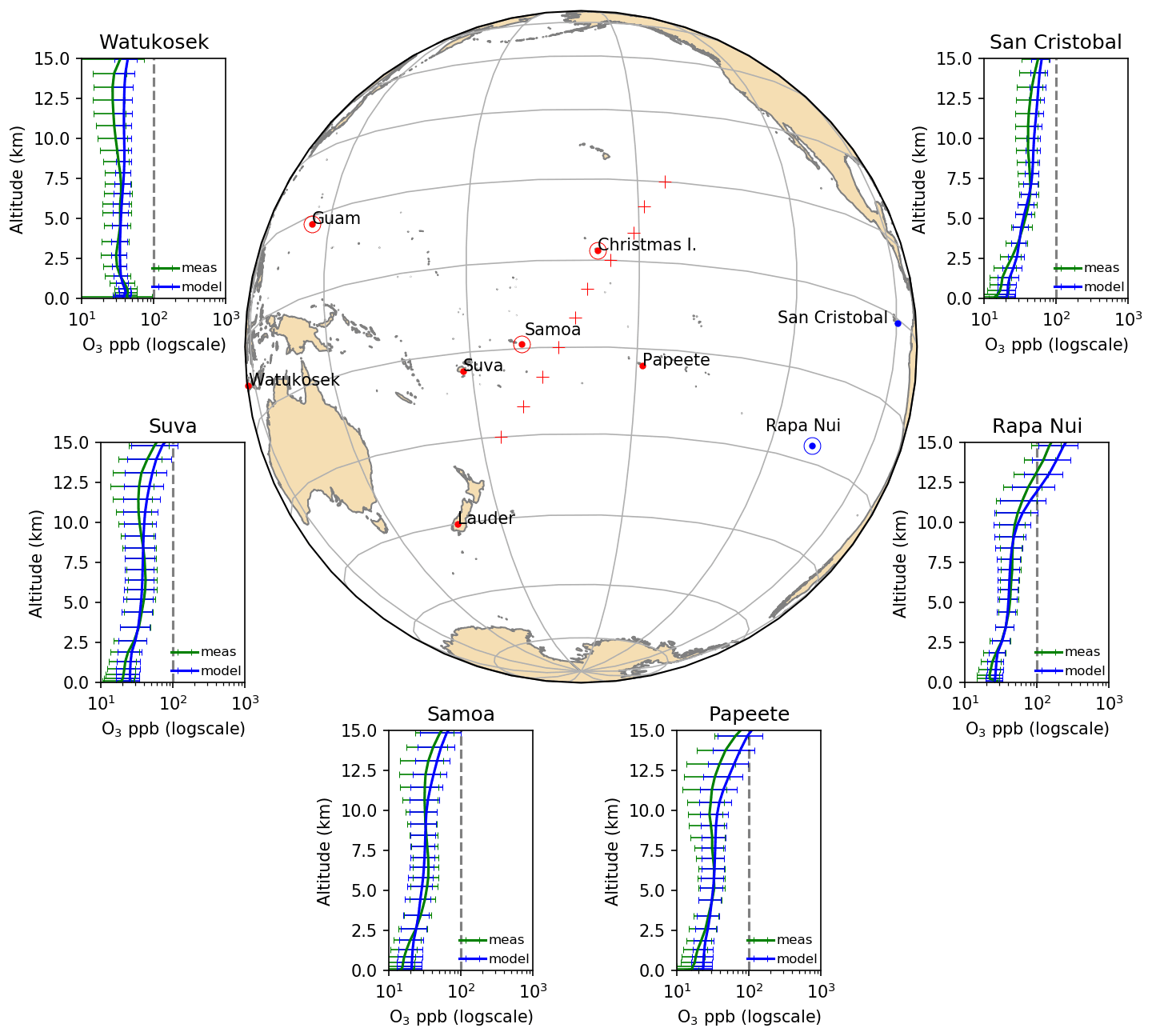
Figure 1Area of study and ozone profile climatologies (1994–2014) as derived from the observations and simulations for six sites in the remote Pacific (red dots). The location of the stations is shown on the map. Also shown are the stations where surface CO measurements were considered (red + symbol). Ozone measurements are shown in green and simulations in blue. The error bars correspond to 1 standard deviation of the mean. The vertical grey line represents the chemical tropopause (100 ppb for the Southern Hemisphere, Prather et al., 2011). The Rapa Nui and Samoa stations, where both O3 and CO observations are available, are marked with a dot and circle. Ozone data were obtained from https://tropo.gsfc.nasa.gov/shadoz/ (last access: 4 December 2018), except for Rapa Nui, which was accessed at http://www.cr2.cl/datos-ozonosonda/ (last access: 23 March 2018). CO data come from https://www.esrl.noaa.gov/gmd/dv/data/ (last access: 2 May 2020).
Despite the above-mentioned progress made in our understanding of tropospheric ozone abundances and precursors in the tropical South Pacific Ocean, no systematic long-term study exists in the literature that integrates the O3 variability over the entire tropical and subtropical South Pacific from west to east. This is important because the western tropical, eastern tropical, and subtropical pristine Pacific areas are affected by air masses originating from multiple distant sources and atmospheric dynamics.
Hence, the present study takes into consideration the entire tropical and subtropical South Pacific Ocean to (a) understand tropospheric O3 variability in this region, (b) understand the drivers of O3 changes due to dynamics (STE and transport) and sources (emissions) and their relative importance, and (c) attribute and quantify the CO enhancement by biomass burning to specific source regions. To pursue the above, ozone observations from ozonesondes and in situ ground-based observations for CO (Fig. 1), alongside satellite observations for both trace gases and a global three-dimensional chemistry-transport model (CTM), were used. The CTM was driven by year-specific assimilated meteorology (ECMWF ERA-Interim for the years 1980–2014) and accounted for tagged CO tracers from biomass burning from the 13 different regions defined by the Hemispheric Transport of Air Pollution (HTAP) task force (HTAP, 2010).
2.1 Modeling
2.1.1 Model description
The model used here is the well-documented, global three-dimensional, offline chemistry and transport model TM4-ECPL. The version of the model used for the present study has been described in detail by Daskalakis et al. (2015, 2016). Thus, hereafter we provide only information that is directly relevant to the present study. The model is driven by the ECMWF ERA-Interim meteorology (Dee et al., 2011), updated every 3 h, and runs at a horizontal resolution of (longitude × latitude), with 34 hybrid vertical layers up to 10 hPa (approximately 65 km).
Most of the model's vertical layers (between 20 and 25, depending on surface pressure) lie in the troposphere, allowing for comprehensive tropospheric calculations. In the stratosphere, the model uses an oversimplified chemical scheme. To account for proper upper-boundary conditions, the O3 concentrations above 50 hPa altitude are nudged to monthly mean observations from the Microwave Scanning Radiometer (MSR) satellite instrument for the years 1980–2008 and the Global Ozone Monitoring Experiment (GOME2) for the years 2009 onwards, interpolated to the model levels by the Royal Netherlands Meteorological Institute (KNMI) (Van Der A et al., 2010). Using the stratospheric ozone concentration, the model calculates nitric acid in the troposphere by applying a ratio derived by the Upper Atmosphere Research Satellite (UARS). The methane (CH4) concentration in the stratosphere is forced to the Halogen Occultation Experiment (HALOE) CH4 climatology (Huijnen et al., 2010). In addition, tagging of stratospheric ozone is performed using a stratospheric O3 tracer that is transported from the stratosphere to the troposphere; within the troposphere the tracer is destroyed by the same photochemical reactions with tropospheric O3 and is also subject to dry deposition (Roelofs et al., 1997).
The model accounts for year-specific emissions of gases and aerosols from anthropogenic and biomass burning sources from the Atmospheric Chemistry and Climate Intercomparison Project (ACCMIP) emission database (Lamarque et al., 2013) up to the year 2000 and from RCP6.0 (Fujino et al., 2006; van Vuuren et al., 2011) from 2001 onwards. In particular, biomass burning emissions vary monthly, and their injection height follows the Aerosol Comparison between Observations and Models (AEROCOM) recommendations (Dentener et al., 2006).
2.1.2 Simulations
To assess the atmospheric composition of the tropical and subtropical Pacific Ocean and its drivers, three simulations were performed. For the first one, the base case simulation, the model runs continuously from 1980 to 2014, saving gridded monthly averaged concentrations of 120 trace gases and aerosol components and hourly gridded three-dimensional fields for selected pollutants (O3, NOx, CO). A spin-up time of 14 years is used to bring the model into dynamic equilibrium between sources and atmospheric concentrations for all species. Therefore, the model output analysis is limited to 21 years, from 1994 to 2014. To assess the impact of large-scale wildfires, a second simulation with omitted biomass burning emissions was performed that was identical to the base simulation in every other aspect.
A third simulation, identical to the base simulation but with the addition of tagged species for biomass burning CO, was used to determine the impact of open fires from different regions on CO levels in the study area. For this, we split the globe into 13 source regions based on the source regions of the HTAP task force (Galmarini et al., 2017; HTAP, 2010). The regions are Europe, northern Africa, southern Africa, Russia, central Asia, Saudi Arabia, India, China, Southeast Asia, Oceania, North America, and South America. For each of the regions, a tracer was added in the model with the same regional biomass burning emissions and the same removal processes as CO through wet and dry deposition and oxidation by hydroxyl radical (OH) but without impacting the concentrations of OH and other chemicals in the model.
2.2 Observations
For the validation of the model results, a set of observations was used to compare the simulated concentrations against. In situ measurements for O3 were obtained from the European Monitoring and Evaluation Programme (EMEP) network for Europe and from the National Oceanic and Atmospheric Administration (NOAA) and the World Data Center for Greenhouse Gases (WDCGG) for the rest of the world. Ozonesonde data were obtained from the Southern Hemisphere ADditional OZonesondes (SHADOZ) database, extended with data for Rapa Nui (Sect. 2.2.1). Carbon monoxide surface measurements were also obtained from NOAA and WDCGG (Sect. 2.2.1). Since the model version used in the present study has been validated against the surface O3 (R=0.48, NMB=17 % with a sample of 2417 measurements globally) and CO (R=0.41, % with a sample of 229 measurements globally) observations around the globe (Daskalakis et al., 2016), the focus here is on the South Pacific regions.
Table 1Ozone sounding stations in the Pacific Ocean considered in this study. Data were obtained from Southern Hemisphere ADditional OZonesondes (SHADOZ, https://tropo.gsfc.nasa.gov/shadoz/, last access: 4 December 2018) and from Rapa Nui from https://www.cr2.cl/datos-ozonosonda/ (last access: 23 March 2018).

∗ m a.s.l.: meters above sea level.
2.2.1 In situ data
We use the SHADOZ database, which is extensively described in the literature (Stauffer et al., 2018; Thompson et al., 2017; Witte et al., 2017, 2018). The focus area is the tropical and subtropical South Pacific, and the measurement sites are shown in Fig. 1. For the present study, 20 years of ozone soundings collected by the Chilean Weather Office at Rapa Nui (Gallardo et al., 2016) have also been taken into account. The locations of the stations (also shown in Fig. 1), together with the number of soundings considered in this study, are summarized in Table 1. For optimal comparison of the modeled data to ozonesonde measurements between 1994 and 2014, hourly model values were sampled for a 3 h period covering each ozonesonde flight, while the measurements were averaged over height to fit the model's vertical resolution for the specific time and date of each ozonesonde flight.
Carbon monoxide (CO) has been measured in flasks collected weekly at several sites around the world over the last 2 decades by NOAA (Novelli, 2014; Petron et al., 2018). These data were recently revised and calibrated, providing a consistent database including weekly and monthly averaged values. Out of this collection, we focus on the analysis of data from Samoa and Rapa Nui in the western and eastern Pacific, respectively. These two sites have long time series for both O3 and CO and are representative of the eastern South Pacific (Samoa) and western South Pacific (Rapa Nui).
2.2.2 Satellite data
The model results are compared to the tropospheric ozone column (TOC) derived from the Ozone Monitoring Instrument (OMI) and the Microwave Limb Sounder (MLS) ozone measurements described by Ziemke et al. (2011). Both the OMI and MLS instruments are on board the Aura satellite with an overpass at 13:30 LT and typical spatial resolutions of 13 km×25 km and 5 km×500 km (×3 km vertically), respectively. These data have been available at https://acd-ext.gsfc.nasa.gov/Data_services/cloud_slice/new_data.html (last access: 21 October 2020) since October 2004.
The Measurements of Pollution In The Troposphere (MOPITT) satellite instrument on board the Terra satellite has been providing data (with a typical spatial resolution of 22 km×22 km at 10:30 and 22:30 LT), including tropospheric CO columns, for nearly 20 years (Deeter et al., 2017). The data product used here is the V7 (Deeter et al., 2019). It contains monthly averaged CO columns for the period April 2000 until the present. These data were obtained from the National Aeronautics and Space Administration (NASA) Langley Research Center Atmospheric Science Data Center (NASA-Langley, 2018).
2.2.3 Assessing trends and variability modes
We assessed the ENSO-driven variability by exploring the linear correlation of deseasonalized and detrended time series of CO and ozone with the bimonthly Multivariate ENSO Index (MEI.v2) (Wolter and Timlin, 2011). This index considers the combined expression of ENSO on sea level pressure (SLP), sea surface temperature (SST), surface zonal winds (U), surface meridional winds (V), and outgoing longwave radiation (OLR) for ENSO conditions from 1979 to the present (https://www.psl.noaa.gov/enso/mei/, last access: May 2021). We chose this multivariate index to account for the multiple processes affecting the whole Pacific Ocean rather than one single aspect during diverse ENSO events. Also, MEI filters out shorter-period variability, such as MJO, which is precluded by the weekly sampling of CO and ozone observations. It is also worth noting that ENSO patterns and teleconnections (impacts) have been subject to changes over the last few decades, which makes the choice of more robust ENSO indices particularly difficult (Capotondi et al., 2014; Hu et al., 2020).
To assess trends, we used the Lamsal et al. (2015) method. This method uses a regression model to split the signal into three components: the seasonal component (harmonic functions), the linear trend component, and the residual component. The method also accounts for an error that considers auto-correlation and length of the monthly time series, as reported by Tiao (1990). To avoid the variability due to the MJO, we consider a bimonthly running average of O3 and CO mixing ratios when estimating trends.
3.1 Climatology for the period 1994–2014
The overall performance of the TM4-ECPL model in its current configuration has been previously thoroughly evaluated (e.g., Daskalakis et al., 2015, 2016; Kanakidou et al., 2012; Quennehen et al., 2016). Here we show and assess the model performance over the study region, namely, the remote South Pacific. To this end, we first describe relevant large-scale circulation patterns, i.e., those capable of transporting the biomass burning outflow to the remote Pacific. Secondly, we characterize how the model reproduces ozone profiles collected over this area of the world for the period 1994–2014. Model-calculated tropospheric columns of ozone and carbon monoxide are then compared to satellite observations.
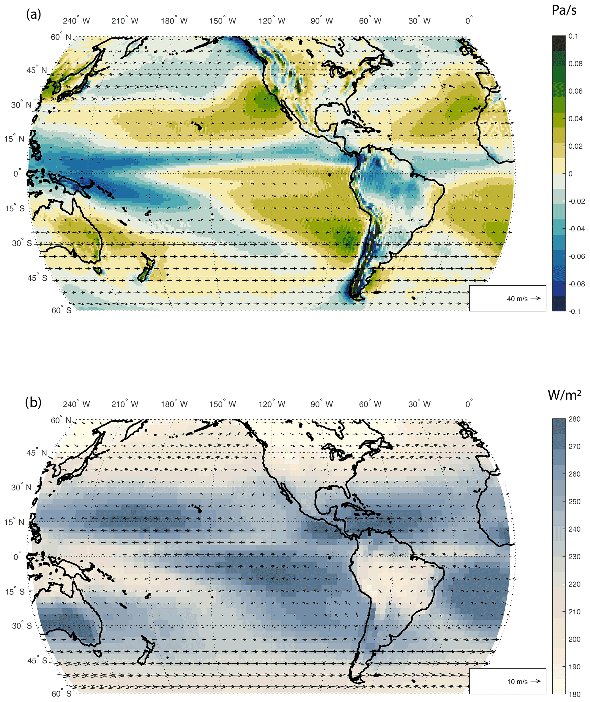
Figure 2(a) Climatological mean of omega vertical velocity (colors in Pa s−1) and 200 hPa winds (vectors) from ERA-Interim reanalysis for the period between 1990 and 2009. (b) NOAA-interpolated outgoing longwave radiation from 1981 to 2010 in W m−2 (colors) and 850 hPa winds (vectors) from ERA-Interim (https://www.ecmwf.int/en/forecasts/datasets/reanalysis-datasets/era-interim, last access: May 2021).
3.1.1 Circulation patterns affecting the remote Pacific Ocean
The main feature of the tropical atmosphere is the Inter-tropical Convergence Zone (ITCZ), which for most of the South Pacific is climatologically located in the Northern Hemisphere (Wodzicki and Rapp, 2016). Therefore, near-surface tropical circulation in the southeastern Pacific is characterized by cross-equatorial northeasterly trade winds. However, since the ITCZ remains mostly over the Northern Hemisphere in the Pacific, the near-surface atmospheric circulation in the tropical and subtropical South Pacific is dominated by the South Pacific Convergence Zone (SPCZ), which consists of a mainly zonal tropical convergence zone and a diagonal subtropical branch that extends from Indonesia down to the mid latitudes of the southeastern Pacific (Brown et al., 2020). The SPCZ is a reverse-oriented monsoon trough that marks the preferential path of energy export from the warm Pacific pool in the tropics to mid latitudes. The SPCZ axis also marks the maxima of the 500 hPa upward vertical motion and the minimum in OLR (Fig. 2a and b). The SPCZ is located at the maximum of low-level convergence and separates the wet warm pool region from the dry subtropical southeastern Pacific, which features the largest values of OLR over the Pacific (Fig. 2b). The SPCZ axis location varies intraseasonally following the MJO, interannually due to ENSO, as well as on interdecadal and longer timescales (e.g., Lintner and Boos, 2019; Vincent, 1994; Vincent et al., 2011). The SPCZ shifts equatorward and becomes more zonal during strong ENSO events (e.g., Brown et al., 2020). In addition, winds blow towards the SPCZ from the northeast in the eastern tropical Pacific and weakly from the west in the western tropical Pacific (Fig. 2b). The upper-level circulation is rather weak in the tropical band and features upper-level divergence which establishes an anticyclone associated with the main tropical convection in the warm pool. South of about 15∘ S, climatological upper-level circulation is mostly zonal with a strong maximum south of the warm pool region where the meridional temperature gradient is at a maximum (Fig. 2a). On a shorter timescale, SPCZ variability is affected by mid-latitude Rossby waves and by tropical waves, in particular by the MJO. MJO phase and intensity have a significant effect on the tropical and extratropical South Pacific weather (through teleconnections) and are responsible for short-term (weekly) changes in weather patterns. Both ENSO and MJO weather patterns affect atmospheric circulation in the South Pacific and thus the transport of pollution into the region.
3.1.2 Climatology of vertical ozone profiles
Figure 1 shows 20-year ozone-sounding climatologies from six sites in the Pacific derived from observations and model outputs. Overall, there is good agreement between observed and simulated ozone profiles when accounting for the temporal variability, while small positive biases are found in the boundary layer (BL) and the upper troposphere (UT) above 8 km when comparing the average values over the entire 20-year period (up to 50 % and 25 %, respectively). Note that the atmosphere above remote oceans is relatively well mixed – due to lack of anthropogenic activity or any natural source presenting large variability, which justifies the comparison of point measurements to the results in the coarse model grid. The lack of halogen chemistry in the current model version may explain the BL bias, in line with modeling studies that show the importance of halogens for O3 depletion in the marine boundary layer (Pechtl and von Glasow, 2007; Sherwen et al., 2016). The UT bias may be attributed to the treatment of the upper-boundary conditions for ozone. In general, the model reproduces the variability of the measurements well (expressed as the standard deviation normalized by the mean), except at Watukosek (Java), where the model variability is much smaller than the one observed (average of 9 ppbv across all altitudes and times for the model against 16 ppb for the measurements). We attribute this mismatch to the vicinity of large and variable sources in Southeast Asia and Australia that result in ozone formation events, the variability of which cannot be captured by the climatological (monthly mean) emissions of ozone precursors used in the model. Another factor contributing to this bias could be the relatively coarse model resolution () that limits the accuracy in the representation of the synoptically driven ozone intrusions. However, the use of reanalysis meteorological data by the model is minimizing this potential bias, and the model is a powerful tool to understand O3 climatology in the study region.
3.1.3 Tropospheric columns of O3 and CO
To further evaluate the model's ability to simulate the long-term variability in tropospheric O3 and CO amounts, we compare the model results to the retrieved tropospheric columns from the OMI for ozone for the period 2004–2014 and total column of CO from MOPITT for the period 2000–2014. To optimize this comparison, we sampled the model at the satellites' overpass times, i.e., at 13:30 LT for O3 and at 10:30 and 22:30 LT for CO. The OMI/MLS product for O3 is publicly available and provided as monthly mean gridded values on a lat–long grid, while for the MOPITT CO product, daily overpasses are available at a 22 km×22 km resolution (at most two per day).
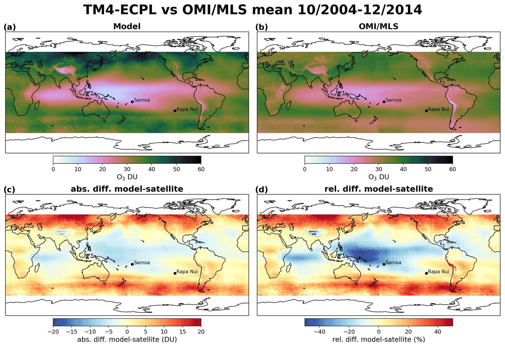
Figure 3Model–satellite comparison between TM4-ECPL and OMI/MLS mean tropospheric ozone column between October 2004 and December 2014. Panel (a) shows the average modeled tropospheric ozone column for the period, panel (b) the average observed tropospheric ozone column, panel (c) the absolute difference between model and satellite (DU), and panel (d) the relative difference (%) between model and satellite in the grid of the OMI. The black dots show the location of Samoa (left) and Rapa Nui (right).
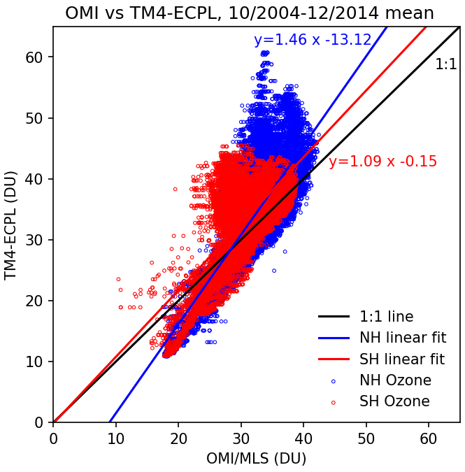
Figure 4Mean tropospheric ozone column of model results versus observations (DU) for the period between October 2004 and December 2014 for all grid cells of shown in Fig. 3. Blue points are NH locations, and red points are SH locations. The black line is the 1:1 line. The red line is the linear fit of all the SH data with the fit equation in red text, where the blue line is the linear fit of the NH data with the fit equation in blue text.
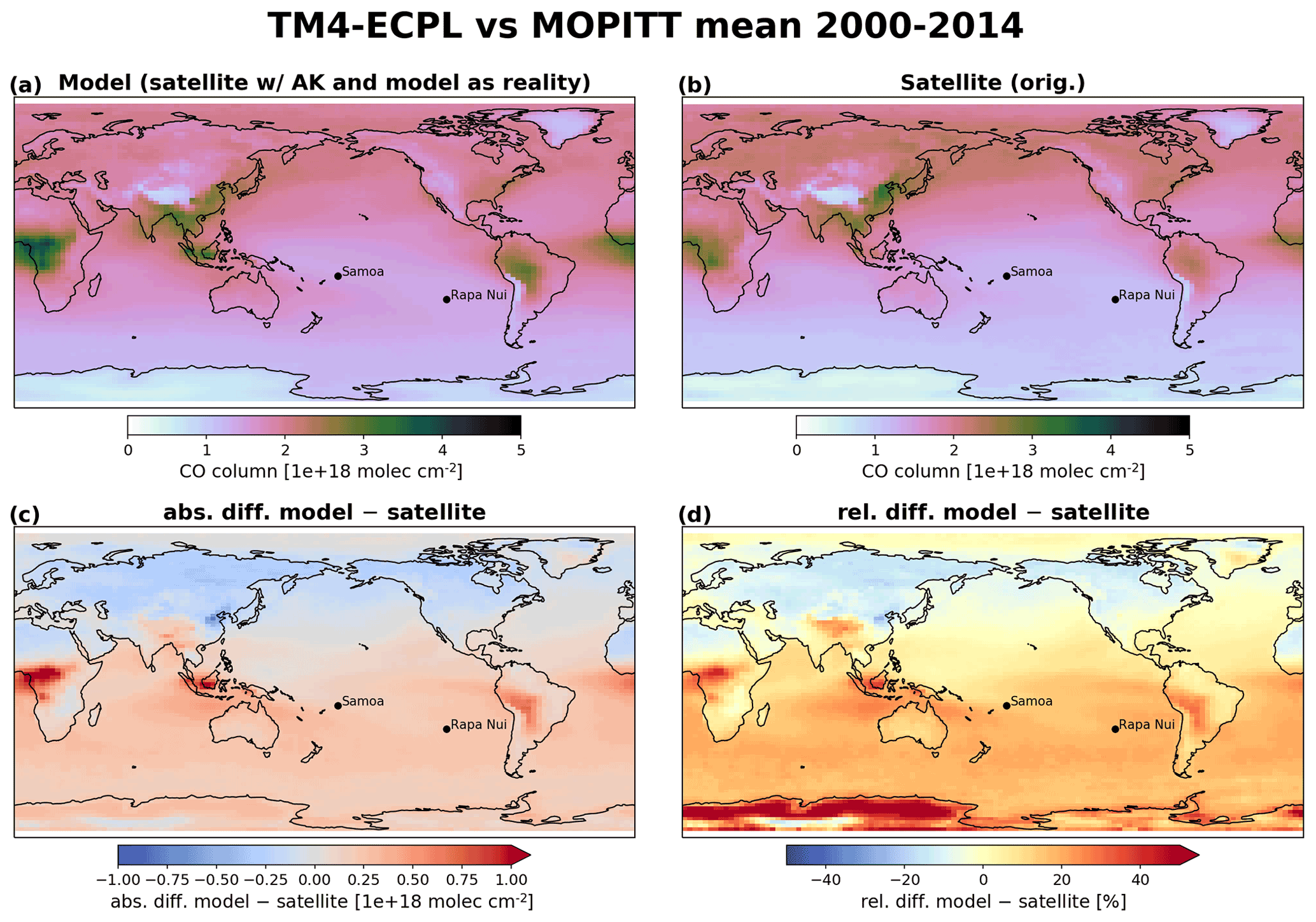
Figure 5Model–satellite comparison between TM4-ECPL and MOPITT for CO total columns averaged from 2000 to 2014 (1018 ). (a) Modeled data sampled following the satellite track and the overpass times and averaged over the period, (b) satellite data averaged over the period, (c) absolute difference (1018 ), and (d) relative difference (%) between the mean values of model results and satellite in the 22 km×22 km grids of MOPITT. The black dots show the locations of Samoa (left) and Rapa Nui (right).
For O3, the model is sampled at the time and location of the satellite overpass and then averaged over the month. For a proper comparison to the OMI product, the tropospheric data are extracted from the model results by calculating the tropopause height based on a lapse-rate threshold as described in Reichler et al. (2003). This way a proper validation of the model against O3 satellite observations (Fig. 3) is achieved. Unfortunately, no information is available on the quality control applied to the OMI/MLS O3 product or for potential missing values. Therefore, the full model dataset at the satellite overpass times (13:30 LT) is extracted, sampled, and used to calculate monthly means for comparison to the satellite observations. Figure 3 shows good agreement between the simulated tropospheric O3 columns and the satellite product which corresponds to a Pearson correlation of 0.66 and a slope of 1.09 for the SH and a Pearson correlation of 0.76 and a slope of 1.46 for the NH (Fig. 4). The main discrepancies are found in highly polluted areas (Beijing region, northern India, eastern USA), where the model calculates higher tropospheric O3 columns by up to 20 DU. These can be attributed to the model's vertical resolution that might not always accurately resolve the tropopause level but also to the fact that the model seems to generally slightly overestimate surface O3 (by about 17 % globally, Daskalakis et al., 2016). Nonetheless, the model seems to capture the climatology of the global tropospheric ozone column, simulating high ozone in the vicinity of polluted areas as well as in the pollution outflows (e.g., southern Africa) that are of interest for the present study. Focusing on the area of interest (5∘ N–40∘ S and 165∘ E–85∘ W), the model seems to perform even better when compared to OMI/MLS, with a Pearson correlation of 0.94, a slope of 1.7, and a normalized mean bias of −3.9 %, showing an underestimation by the model over this region.
For the comparison to the CO MOPITT data, after sampling the model at the time and place of the observation, the results are weighted by the averaging kernel used for the MOPITT CO retrievals. This method leads to a model-derived product directly comparable to the satellite product and is shown in Fig. 5. Thus, the model is validated against daily CO data. CO data from MOPITT are compared against the modeled tropospheric CO column (Fig. 5). The calculated tropospheric CO columns derived using the averaging kernel of the observed data on the simulated data correspond to what the satellite would have observed if the model were an accurate representation of the reality. The model results are collocated to the observations, applying a quality control filter to both the modeled and observed data so that the comparison is accurate (i.e., we disregard values where the model surface pressure has a difference of more than 5 hPa compared to the retrieved data, and we disregard all the retrieved data that are flagged as anomalous, meaning that these data should either be ignored or used cautiously). The comparison gives a very good agreement between model and satellite observations at spatial resolution, with a Pearson correlation of 0.93 and a slope of 0.8 for the period between 2000 and 2014 (15 years of daily collocated data) globally. Over the area of interest (5∘ N–40∘ S and 165∘ E–85∘ W), the model performs well with a Pearson correlation of 0.91 and a slope of 1.0. Further investigation of the differences between the observed and simulated CO concentrations reveals that the model overestimates CO over large wildfire regions of the Southern Hemisphere (southern Africa, South America, Indonesia), where differences between satellite and model tropospheric columns can reach up to 30 %. Over the subtropical Pacific Ocean, these differences are below 10 %. However, CO long-term variability is captured by the model, as shown by Daskalakis et al. (2016) for continental sites and as discussed further for the South Pacific region (Sect. 3.2.2).
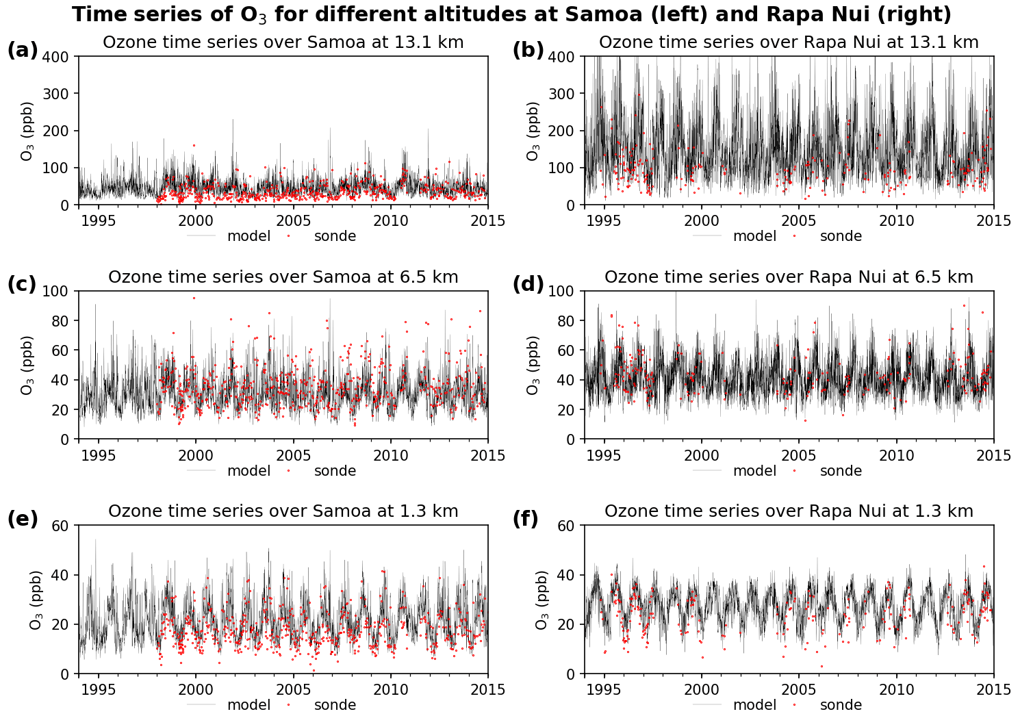
Figure 6Time series of ozone in the boundary layer (1.3 km, e and f), mid troposphere (6.5 km, c and d), and upper troposphere and lower stratosphere (13.1 km, a and b) as derived from the model (black lines) and ozonesonde measurements (red dots). Data correspond to the period between 1994 and 2014 at Samoa (a, c, e) and Rapa Nui (b, d, f).
3.2 Variability and trends
In the previous section, we analyzed the climatology (long-term averages) of ozone and carbon monoxide. Here, we address seasonal and interannual variability patterns and to what extent the simulations capture them. The main drivers of variability are the temporal variations of emissions and photochemistry and atmospheric dynamics that affect long-range transport and downward flux from the stratosphere. In the case of ozonesondes, the comparison is made for daily data, whereas in the case of CO, we use monthly averaged data.
3.2.1 Ozone variability as shown by ozonesondes
For this analysis, we choose one representative station on each side of the Pacific Ocean, where there is an abundance of measurements to assess the observed and simulated ozone variability in the region. Figure 6 shows the comparison between model and ozone soundings over the eastern and western Pacific, represented by stations Rapa Nui and Samoa, respectively. We show the time series at 1.3 km (Fig. 6e and f), 6.5 km (Fig. 6c and d), and 13.1 km (Fig. 6a and b) altitude as representative of the boundary layer, mid-troposphere, and upper-troposphere/lower-stratosphere (UTLS) regions, respectively. The positive model bias near the surface and in the UTLS shown in Fig. 1 is also evident here. However, the overall variability of the time series is well captured by the model, particularly in the mid and lower troposphere, with Pearson correlations between 0.69 and 0.91 (Table 2). Only over Rapa Nui does the upper-boundary condition translate into a poorer model performance with a normalized mean bias of 67 %. Both stations show a marked seasonal cycle, with maxima (minima) in spring (fall) at all levels, as well as interannual variability.
Table 2Error statistics for model simulation versus observations of monthly averaged O3 for Rapa Nui and Samoa in the remote Pacific at three altitude levels. We show Pearson correlation (R), root mean square (rms – ppbv), normalized mean bias (NMB – %), and index of agreements (IA). The number of data points considered is also indicated. Calculations were made according to Brasseur and Jacob (2017).
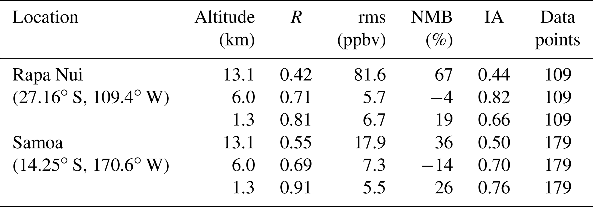
Table 3Estimated decadal ozone trends (ppbv per decade) at different altitudes over Rapa Nui and Samoa in the Pacific Ocean according to observations and simulations for the period 1994–2014. Trends based on model values are calculated using all data points (“Model”) and only those for which there are concurrent observations (“Model∗”). Trends are calculated following Lamsal et al. (2015) and errors as in Tiao (1990). The number of data points (N) considered is also indicated. Trends and errors are in ppbv per decade.

Using the Lamsal et al. (2015) approach, we estimated trends for observed and simulated ozone soundings on a bimonthly basis (see Table 3). Over Rapa Nui, one finds a clear positive trend (0.5±0.1 ppbv per decade) in the boundary layer observations, which is consistent with previous results (Gallardo et al., 2016). The model, on the other hand, indicates either a clear negative trend ( ppbv per decade) when considering all data points or a negligible or statistically insignificant trend when considering only months with concurrent observations. This finding suggests that local pollution – not represented in the model – may in fact be affecting near-surface ozone as proposed by Gallardo et al. (2016). However, other factors cannot be ruled out. In the mid troposphere, the observations indicate a marginally negative trend where the model shows decreasing ozone values ( ppbv per decade). A negative trend is expected in connection with the widening and weakening of the Hadley circulation in a warming climate (Hu et al., 2018; Lu et al., 2019). However, the magnitude of the decline is obscured by the possibly overestimated role of STE in the upper troposphere in the model simulations. Interestingly, the model results concurrent to observations at 13.1 km are quite similar, although an improvement in the performance of the model is found towards lower altitudes (see Tables 2 and 3). Furthermore, the intermittence of ozone soundings over the southeastern Pacific in this period hampers a definite assessment.
Observations over Samoa show marginally declining trends in near-surface ( ppbv per decade) and a declining non-significant trend in mid-tropospheric ozone ( ppbv per decade). These changes are in line with the recent findings by Thompson et al. (2021) for the period 1998–2019. TM4-ECPL reproduces the sign of the trend in the mid troposphere but overestimates the magnitude when considering all data points as well as for the data points with concurrent observations (see Table 3). It performs well at 1.3 km when compared to concurrent observations (see Tables 2 and 3). In the upper troposphere, the observations show a strong increasing trend (2.6±0.3 ppbv per decade), larger than the trend computed by Thompson et al. (2021). There, depending on the number of data points considered, TM4-ECPL calculates either a marginally positive trend (all model data) or a negative trend (concurrent data only), the reason probably being the different number of ENSO occurrences covered by the two model datasets. An explicit representation of stratospheric chemistry in the chemistry-transport model as well as longer observed and simulated time series of O3 would enable a more accurate estimate of the trends in UTLS O3 as well as of the influence of ENSO.
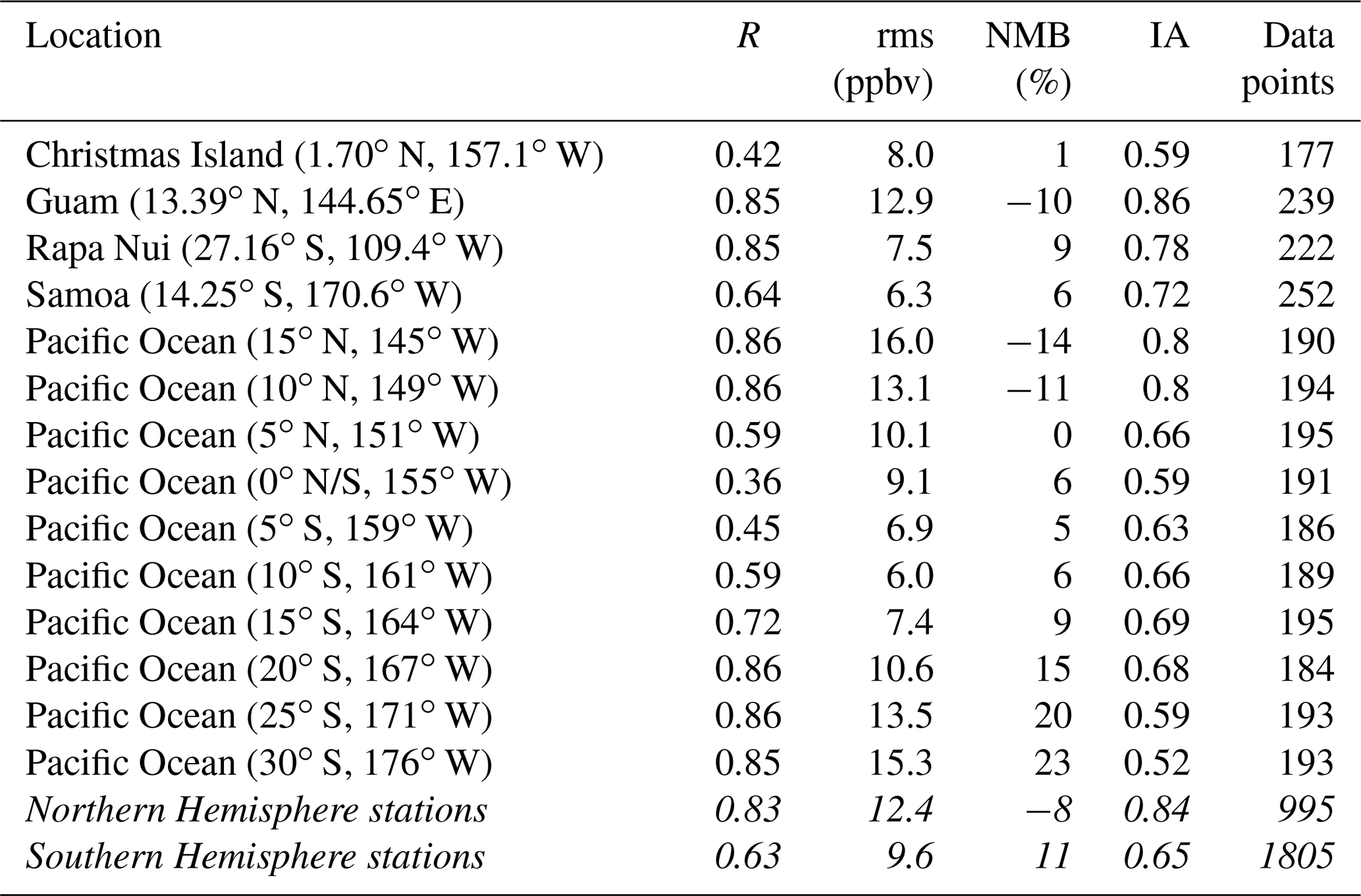
Table 4Error statistics for model simulation versus observations of CO for 14 stations in the remote Pacific. Per definition, these indexes are calculated for data points where both observations and simulations are available over the period 1994–2014. Symbols are as in Table 2.
With respect to the ENSO-driven variability as expressed by the correlation with the MEIv2 index, observations of mid-atmospheric ozone over Rapa Nui show a positive correlation during La Niña years (+0.36); however, the correlation is not statistically significant at a 90 % confidence level. This positive correlation is nevertheless consistent with a strengthened South Pacific high and increased subsidence. There are very few observations at 6 km during El Niño years, which hampers our analysis. The model, on the other hand, shows a negative but significant correlation (−0.30) during La Niña and a positive and significant but weak correlation during El Niño (0.22) (at a 90 % confidence level). The latter is expected as the South Pacific high, and thus subsidence, weakens in El Niño years. The former may be due to too strong an influence of photochemistry compared to that of dynamics in the model despite the model's positive bias in the UTLS.
Over Samoa, where O3 levels are dominated by photochemistry, the observations show a positive correlation (0.33) during El Niño years linked to increased precursor emissions from biomass burning originating mostly from Southeast Asia and a small negative correlation (−0.13) during La Niña years in connection with lesser emissions of ozone precursors in the Southern Hemisphere. However, this is not statistically significant (at a 90 % confidence level), stressing the need to consider long time series to assess ENSO variability robustly. The model evidences a weaker but still positive and significant correlation during El Niño (0.23) and a clear negative correlation during La Niña.
3.2.2 CO variability as shown by flask measurements
The comparison between CO in situ observations and model results (Fig. 7) evidences a general overestimate of CO mixing ratios from the model in the South Pacific Ocean and a general underestimate of CO observations in the North Pacific Ocean. The corresponding mean bias is 7.6 ppbv (8 %) and −6.4 ppbv (−11 %) for the South Pacific and North Pacific Ocean stations, respectively. Both observations and model results show lower mixing ratios in the SH than in the NH. These features are illustrated in a scatter plot in Fig. 7, where models versus observations at 14 stations (see Fig. 1) are summarized. Further error statistics are shown in Table 4. Except for the root mean square error, the model performance is better for stations in the Northern Hemisphere than in the Southern Hemisphere of the remote Pacific.
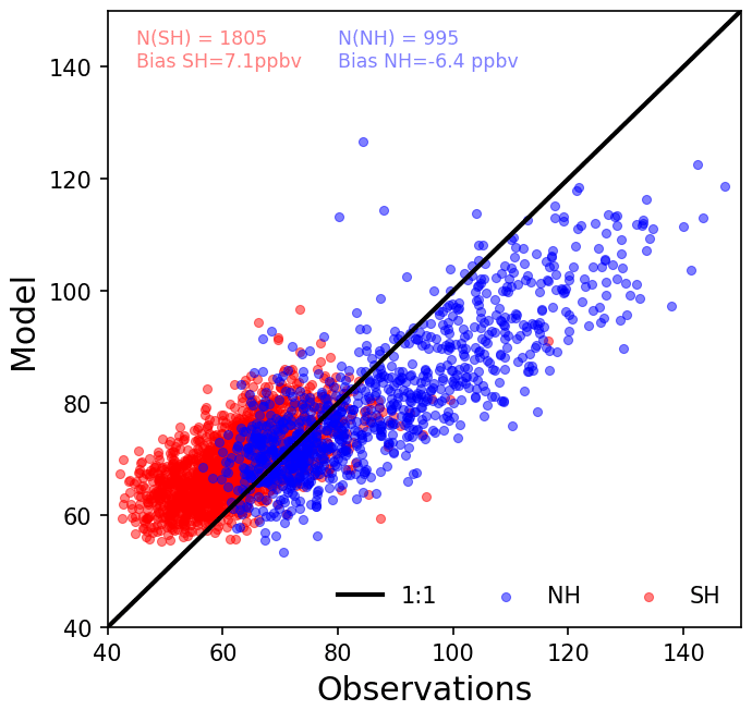
Figure 7Comparison between monthly averages of simulated and observed surface CO at 14 stations in the Pacific (see Table 4). We show in red stations in the Southern Hemisphere (SH) and in blue stations in the Northern Hemisphere (NH). Also shown are the model bias over the SH and the NH and the number of data points considered. For reference, we draw the line 1:1.
Figure 8 shows the monthly mean time series of CO at Samoa (western South Pacific) and Rapa Nui (eastern South Pacific). The model reproduces the seasonality and the interannual variability of the CO observations, albeit with positive biases of 6 % for Samoa and 9 % for Rapa Nui, particularly in the low values of the austral spring. Pearson correlation is better at Rapa Nui than in Samoa (0.85 and 0.64, respectively), whereas the root mean square errors are somewhat smaller for Samoa than for Rapa Nui (6.3 for Samoa and 7.5 for Rapa Nui). This might be linked to inaccuracies in the biomass burning emissions, as revealed from the comparison to satellite observations (see Sect. 3.1.3).
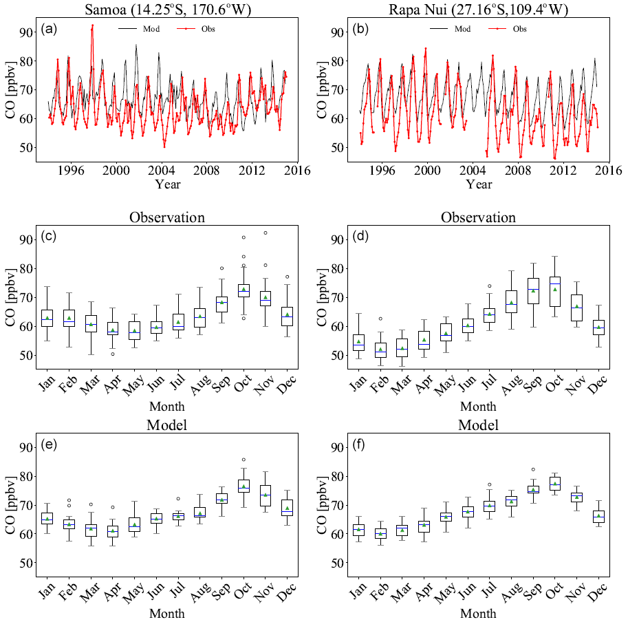
Figure 8Time series (a, b) of observed (red line) and simulated (blue line) CO volume mixing ratios for Samoa (left) and Rapa Nui (right). The seasonal variability is depicted in box plots as shown by observations (c, d) and the simulation (e, f) for CO for the same stations. Boxes show the 25th to 75th percentiles of the data. Whiskers show the 0th and 100th percentiles, excluding outliers. Circles show outliers, the green triangle is the average, and the blue line is the median of each monthly distribution.
The variability of observed surface mixing ratios of CO over the Pacific is not strongly modulated by ENSO over the period 1994–2014 (see Table 5). An exception is Guam (13.4∘ N, 144.7∘ E), which is closest to the outflow of biomass burning from Indonesia. In Guam, ENSO explains ca. 60 % of the observations' and model's variability in the period 1994–2014. There, during El Niño years, positive CO anomalies are found due to increased emissions from fires in Indonesia. The opposite happens during La Niña years. All other stations show a weak correlation with ENSO in the observations. This behavior is coherent with the findings of previous studies, according to which CO variability is mainly driven by emission changes, and with relatively localized impacts (Inness et al., 2015).
Table 5Pearson correlation (R) and number of data points (N) for bimonthly averaged CO values versus the MEIv2 index. In the “Observations” column, we show the calculation for observed CO versus MEIv2. Under “Model”, we show the corresponding calculation considering the continuous series of CO values simulated with the model. Under “Model∗”, we consider model outputs only for those cases when there are CO observations.
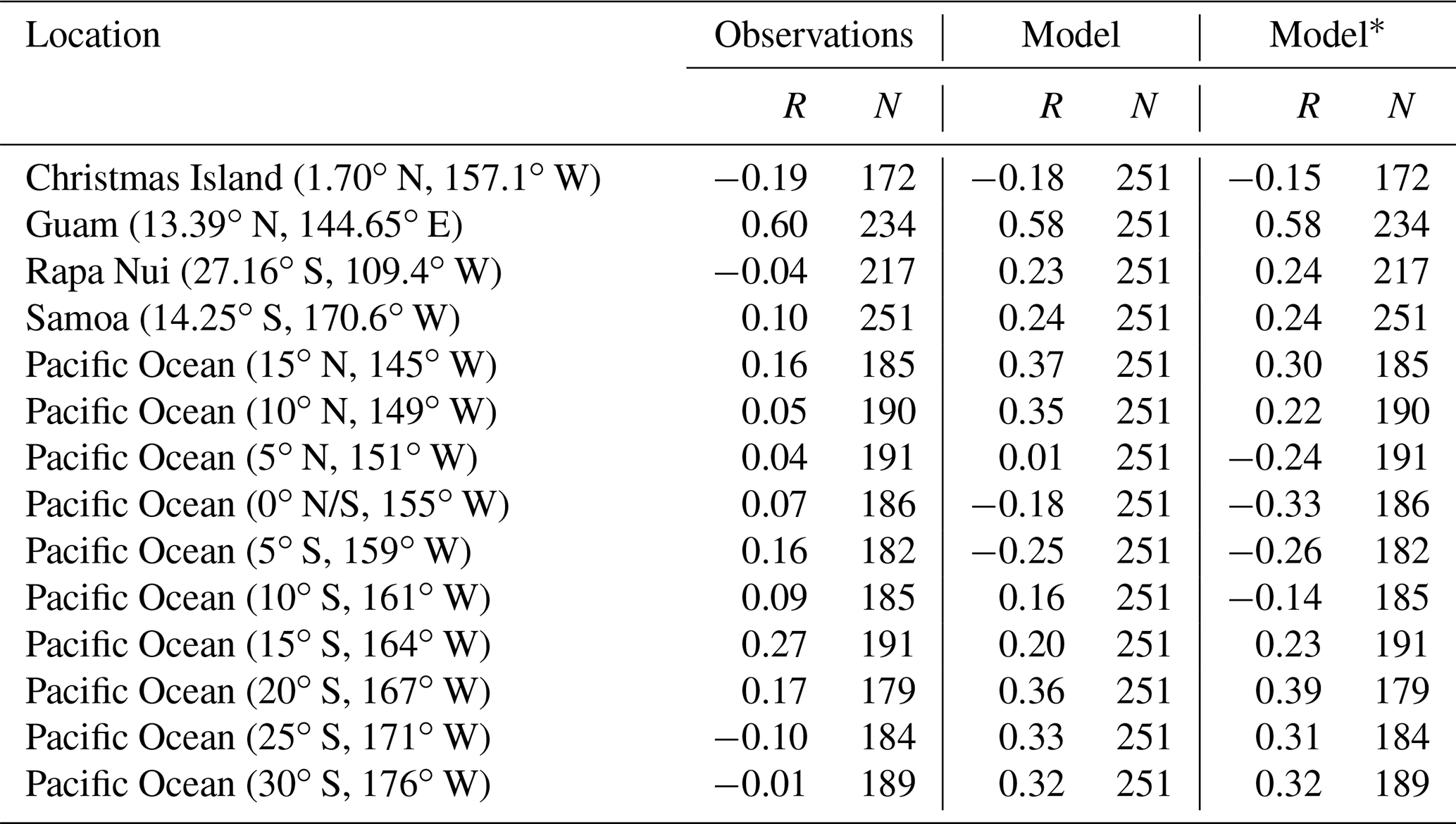
On the other hand, the simulated CO shows higher ENSO modulation than the observations as shown by the Pearson correlations in Table 5. The Pearson correlation between observed CO and MEIv2 is generally weaker than that found between simulated CO and the ENSO index. We hypothesized that this might be due to under-/over-representing the number of ENSO occurrences in the observations over the period 1994–2014. However, the simulated CO still shows a stronger Pearson correlation than the observations when considering the same months when there are observations, except in the mid-Pacific stations – 15∘ N, 145∘ W; 10∘ N, 149∘ W; 5∘ N, 151∘ W; 0 N/S, 155∘ W – where considering fewer data points brings relatively large changes in Pearson correlation. Thus, the relatively weaker Pearson correlation calculated over the observations than over simulated CO indicates other reasons at play. Since we are using reanalysis meteorology, we attribute this mismatch to an ENSO-driven variability in emissions that is not fully captured by the model or to shortcomings in the transport of those emissions.
Table 6Estimated trends of surface CO in the Pacific Ocean according to observations and model outputs for the period 1994–2014. Trends are calculated following Lamsal et al. (2015) and errors as in Tiao (1990). The number of data points (N) considered is also indicated. Trends and errors are in ppbv per decade.
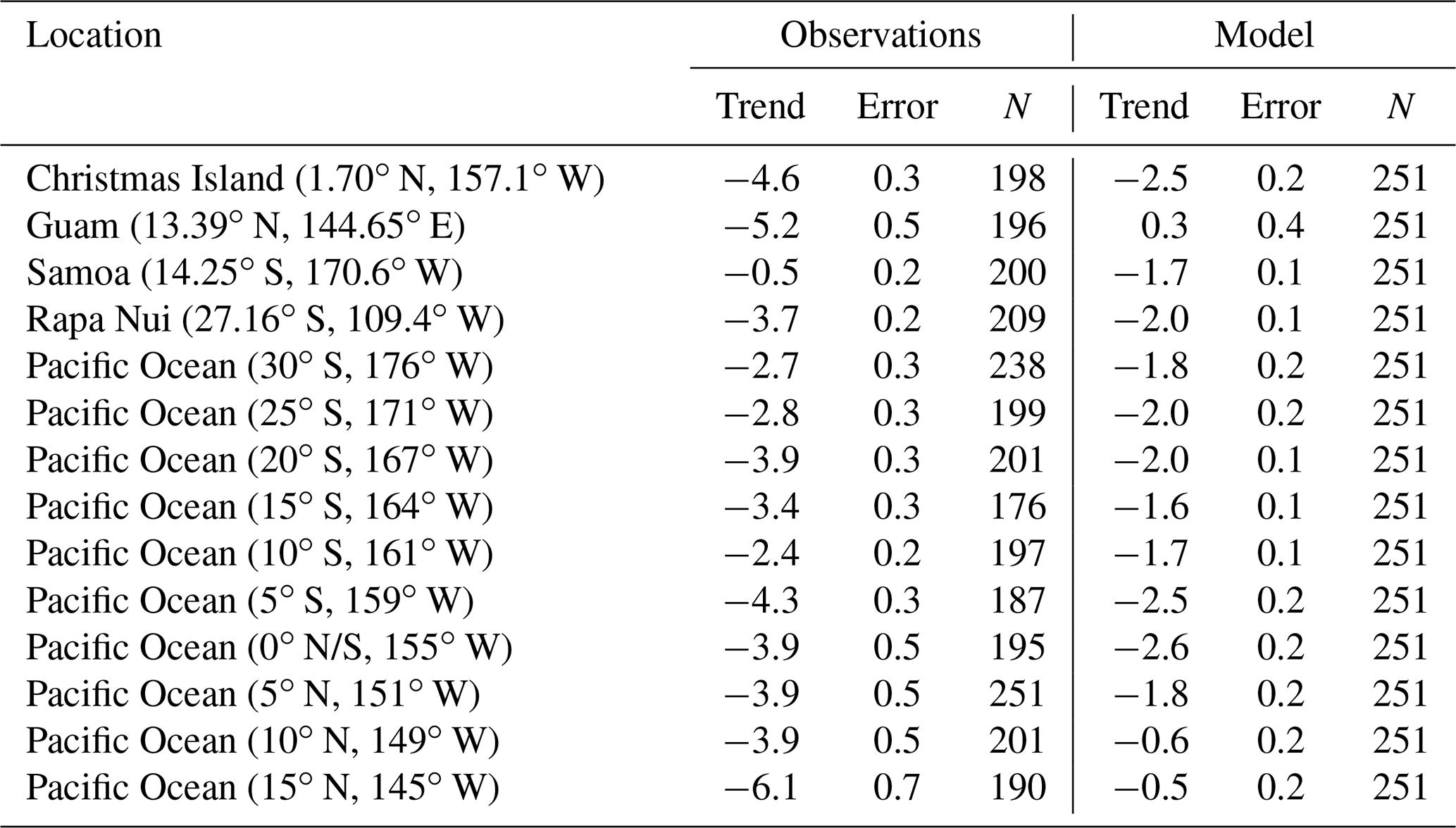
The observations show statistically significant decreasing trends in surface CO for all stations over the period 1994–2014 (see Table 6), except for Samoa, where the trend is marginally significant. The simulated CO also shows decreasing trends but with weaker rates, typically half of those observed. In the northwestern Pacific, model trends are small and marginally significant. The overall decreasing trends are expected in light of the reduction of anthropogenic emissions of CO due to applied legislation for clean air as well as the associated changes in hydroxyl radical concentrations and CO production by methane oxidation (Daskalakis et al., 2016; Gaubert et al., 2017).
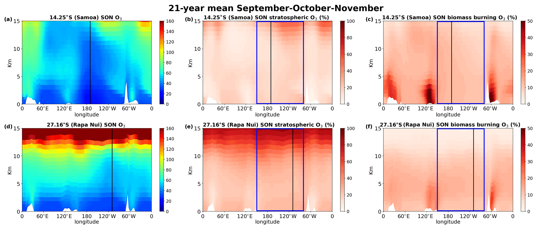
Figure 9Cross section of the 1994–2014 average atmospheric concentration of O3 at the latitude of Samoa (a–c) and Rapa Nui (d–f) for Southern Hemisphere spring (September–October–November) as calculated by the TM4-ECPL. The left column shows the O3 mixing ratio, the middle column the percentage of O3 originating from the stratosphere, and the right column the percentage contribution of biomass burning to the O3 concentrations (note that the third column scale is up to 50 %). The black vertical lines indicate the location of Samoa in the upper panels and Rapa Nui in the lower panels, and the blue rectangle encloses the region of interest.
3.2.3 Stratospheric intrusions, biomass burning impact, and transport pathways
Figure 9 shows the cross section (longitude over height) at 14∘ S (Samoa, tropics, a–c) and 27∘ S (Rapa Nui, subtropics, d–f) for the 21-year mean O3 concentrations (a and d), the stratospheric O3 contribution (b and e), and the biomass burning contribution to O3 (c and f) for the burning period of the SH (September, October, November; SON), highlighting the region of interest with the blue rectangle. The stratospheric O3 is a tagged species in the model tracing the ozone that originates from the stratosphere. The biomass burning contribution is derived as the difference between the base simulation and the simulation without biomass burning emissions (deltaO3). In Fig. 9a (14∘ S), the chemical tropopause (O3 of about 100 ppbv for the SH, Prather et al., 2011) is not evident, while in Fig. 9d (27∘ S), the tropopause is seen at around 13 km. This difference in tropopause altitude between the two locations is expected since 14∘ S (Fig. 9a) is in the tropics closer to the ITCZ, the region where the tropopause is highest (i.e., around 16 km, which is beyond the scale of the figure). In addition, in Fig. 9d, a difference in the tropopause height is observed between the western (around 150∘–170∘ E) and eastern (around 110∘–80∘ W) Pacific (about 2 km lower in the west). The tropopause height also impacts the quantities of ozone penetrating from the stratosphere to the troposphere (Fig. 9b and e), which are almost double at 27∘ S compared to 14∘ S. The 27∘ S is affected by the downward branch of the Hadley cell, resulting in an enrichment of the mid troposphere by about 15–20 ppbv of stratospheric O3. By contrast, in the tropical South Pacific, this enrichment of the mid troposphere is about 7–10 ppbv. During the high burning season (SON), the O3 produced by the chemical aging of biomass burning emissions is higher in the tropics than in the subtropics. However, focusing on the Pacific Ocean region (longitudes between 150∘ E and 80∘ W), we can see that there is a higher contribution of biomass burning to O3 levels (about 3 ppbv more) in the subtropics (Fig. 9f) than in the tropics (Fig. 9c). This enhancement is most evident over the entire subtropical South Pacific except for the BL of the eastern South Pacific. This is caused by the transport patterns of the region that are driven by the tropical Hadley cell circulation with an upward convective flow at the ITCZ and downward fluxes in the subtropics. Southern westerlies dominate air flow at these latitudes. Figure 10 is the same as Fig. 9 but for the low burning period of the South Pacific region (March, April, May; MAM) showing the importance of STE for O3 concentrations, which is larger at Rapa Nui than in Samoa as for SON.
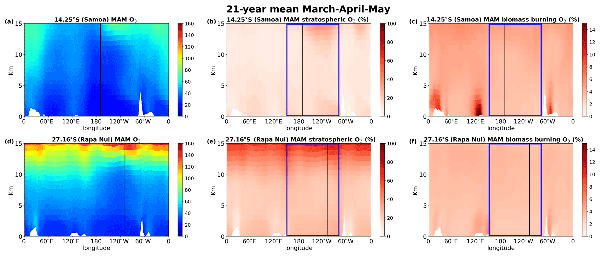
Figure 10As in Fig. 10 but for Southern Hemisphere fall (March–April–May). Note that the third column scales up to 15 %.
Overall, STE is more important than the biomass burning contribution to O3 levels in the free troposphere over the tropical and subtropical Pacific Ocean. However, during SON biomass burning is almost as important as STE in the subtropical boundary layer. During the low burning period, the influence of biomass burning is seen in the high troposphere due to atmospheric transport patterns, as further discussed.
The use of tagged CO tracers enables the identification of biomass burning source areas that contribute to the CO levels in the South Pacific during the intensive burning period (SON) in the region. Figure 11 depicts the simulated vertical profiles of CO at the Samoan and Rapa Nui islands from the surface to 15 km altitude for the high burning period (SON) over the 21-year period studied here. It also shows the contribution to the atmosphere above the islands from all biomass burning sources and the major individual biomass burning source regions to the CO levels in these remote regions in the South Pacific. From this analysis, it is evident that open fires from Southeast Asia are the major contributors to CO from biomass burning at around 12 km, both over Samoa and over Rapa Nui. At lower altitudes, open fires from South America and southern Africa also directly influence the local CO levels. Notably, South America and southern Africa have a larger influence on CO at Rapa Nui than at Samoa. This influence maximizes in the lower troposphere (i.e., at about 3–4 km). Overall, the biomass burning sources contribute 13 % to 27 % to CO concentrations at Rapa Nui and 13 % to 30 % at Samoa, depending on altitude. More specifically, according to the simulations, biomass burning is responsible for a median contribution of 16 % of surface CO over Rapa Nui and Samoa. Interestingly, over both sites, the largest contribution (ca. 40 % of total biomass burning CO) emanates from southern Africa due to circulation patterns connecting the African outflow with the subtropical westerly flow over the Pacific. The second-largest contributing biomass burning source area is Southeast Asia, which is responsible for 33 % of biomass burning CO in Samoa and 21 % in Rapa Nui. Transport from this source region to the South Pacific occurs in connection with the Equator-crossing flow and uplifting associated with the SPCZ. South American biomass burning affects both Rapa Nui (17 %) and Samoa (12 %). Over Rapa Nui, the contribution occurs mainly in connection with the tropical high-altitude easterly flow after convective uplifting over tropical South America. Over Samoa, this contribution emerges from the Atlantic outflow of the South American continent, followed by its confluence with westerly flow at higher latitudes.
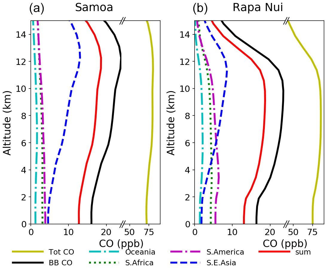
Figure 11Vertical distribution of CO from different source regions (see legend) in Samoa (a) and Rapa Nui (b) for the high burning period (September–October–November). Total CO represents the contribution of all sources of CO, whereas biomass burning (BB) CO represents the sum of all biomass burning sources. The line in red (sum) indicates the sum of all individual BB contributions shown.
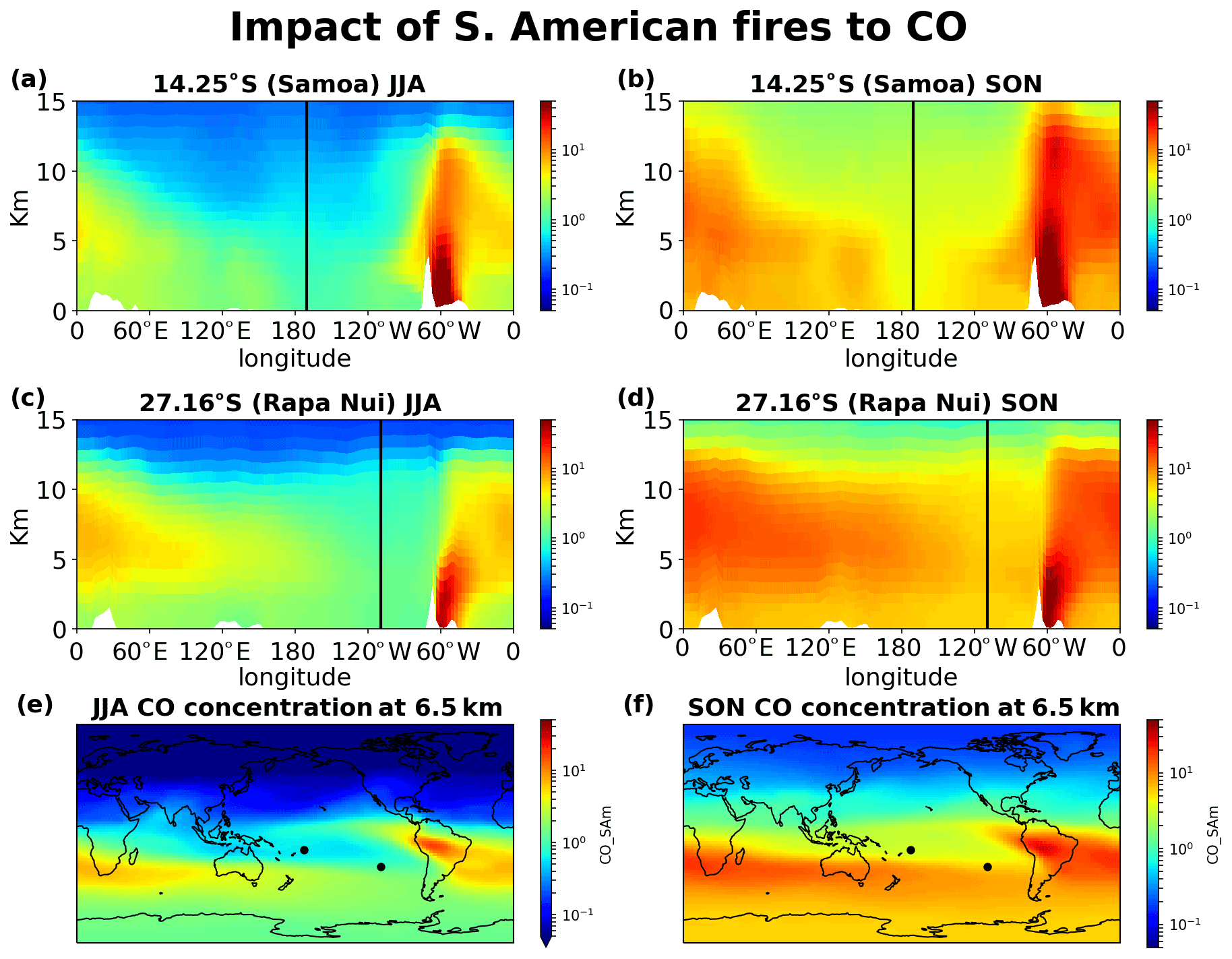
Figure 12Impact of South American fires on CO concentrations. (a) JJA and (b) SON 20-year mean impact at the cross section of Samoa, (c) JJA and (d) SON at the cross section of Rapa Nui, and (e) JJA and (f) SON horizontal distribution of the contribution at 6.5 km altitude.
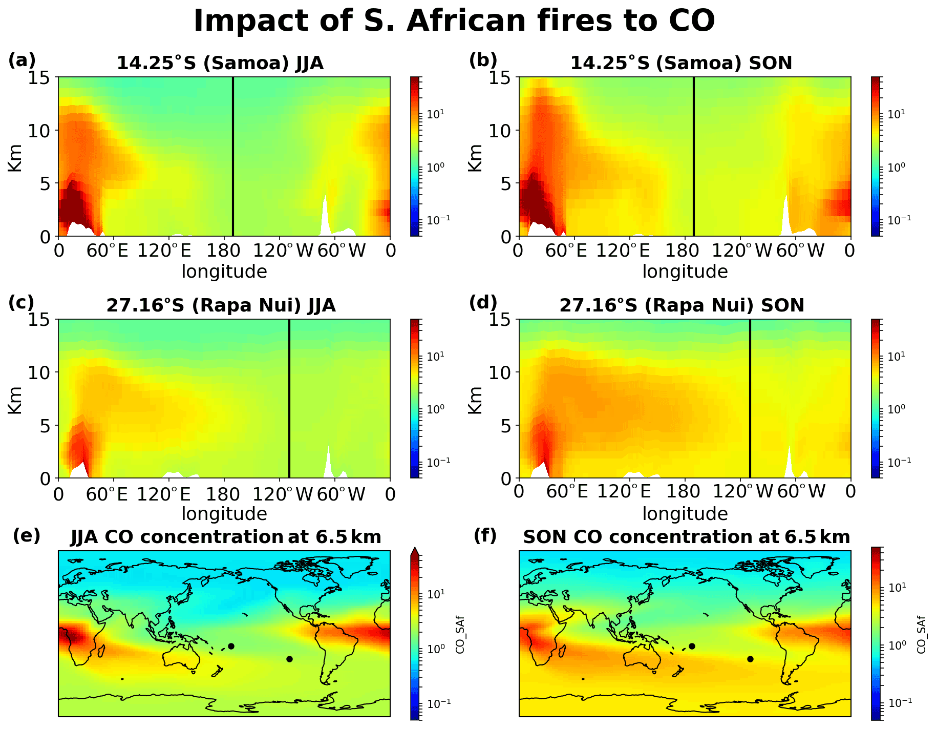
Figure 13Impact of southern African fires on CO concentrations. (a) JJA and (b) SON 20-year mean impact at the cross section of Samoa, (c) JJA and (d) SON at the cross section of Rapa Nui, and (e) JJA and (f) SON horizontal distribution of the contribution at 6.5 km altitude.
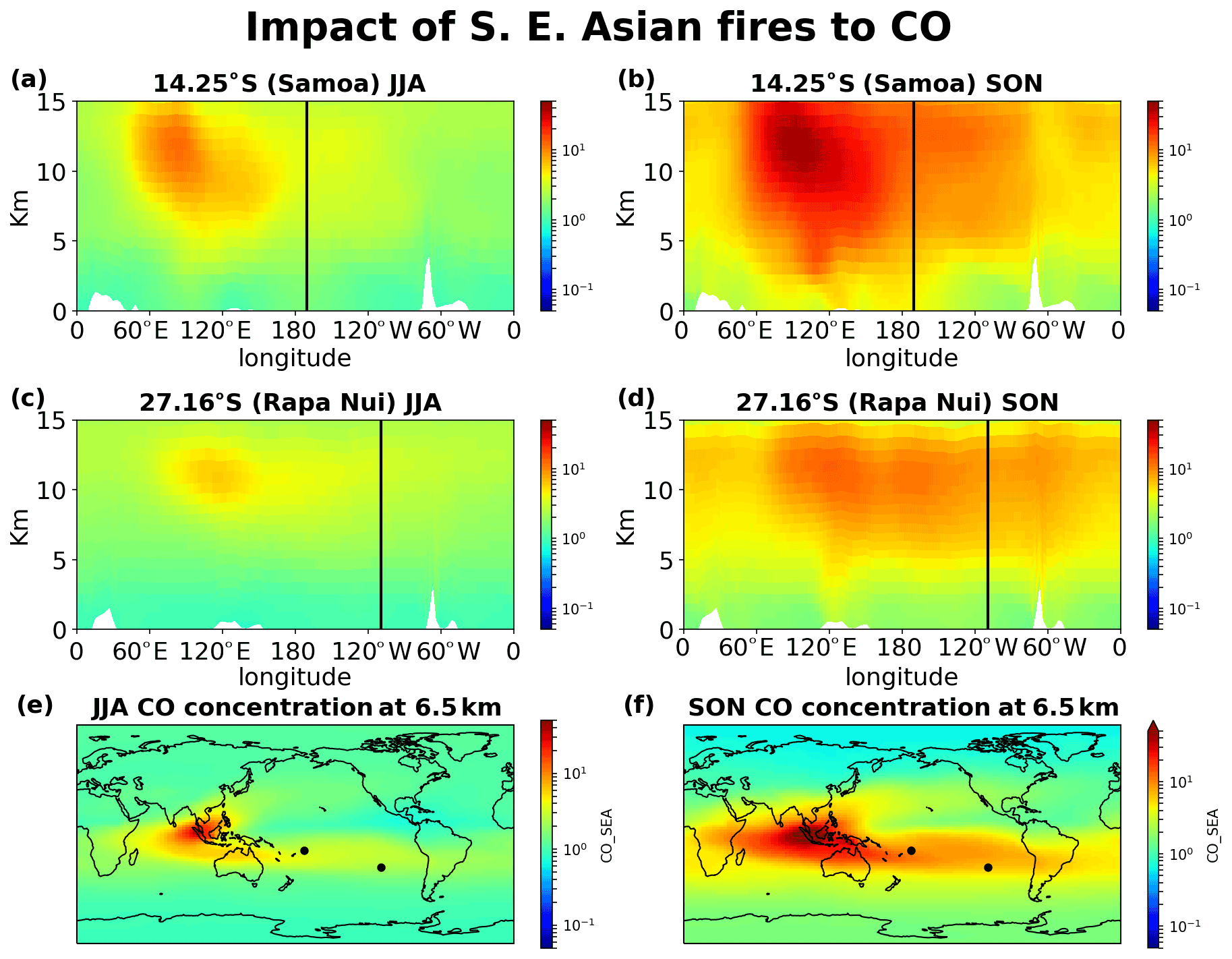
Figure 14Impact of Southeast Asian fires on CO concentrations. (a) JJA and (b) SON 20-year mean impact at the cross section of Samoa, (c) JJA and (d) SON at the cross section of Rapa Nui, and (e) JJA and (f) SON horizontal distribution of the contribution at 6.5 km altitude.
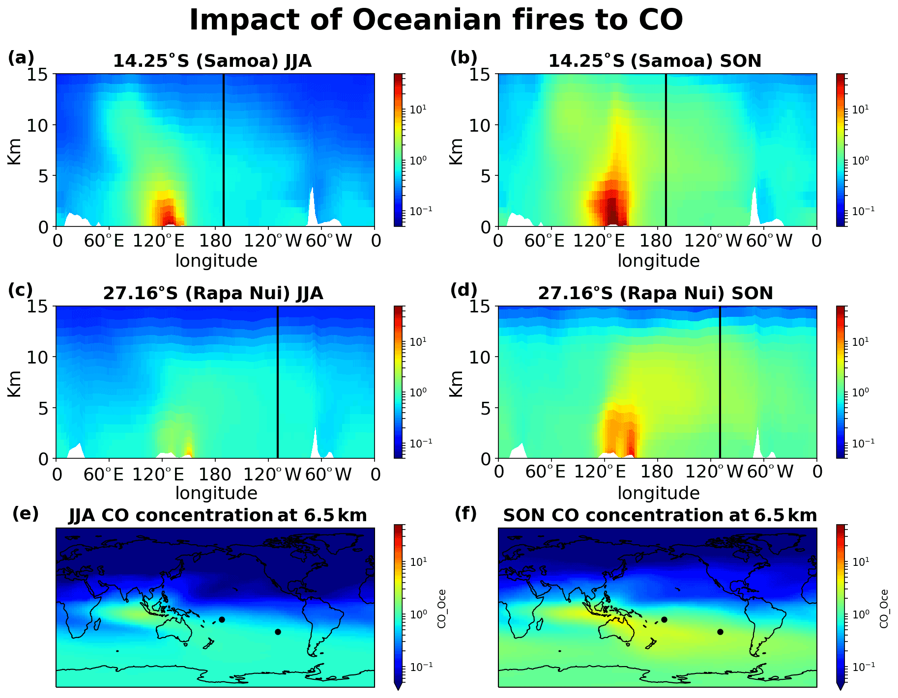
Figure 15Impact of Oceanian fires on CO concentrations. (a) JJA and (b) SON 20-year mean impact at the cross section of Samoa, (c) JJA and (d) SON at the cross section of Rapa Nui, and (e) JJA and (f) SON horizontal distribution of the contribution at 6.5 km altitude.
Figures 12–15 demonstrate the global impact of biomass burning sources. They depict the contribution of biomass burning from the main source regions affecting the tropical South Pacific Ocean free troposphere and UTLS region (5–12 km height) for June, July, August (JJA) and September, October, November (SON), when the impact of the fires maximizes. They also show that wildfires close to the ITCZ have a dual outflow. South American fires are transported westward and affect the tropical eastern Pacific (Fig. 12). Eastward, through transport over the Atlantic and then the southern Indian Ocean, they reach the western subtropical Pacific (Samoa) and, finally, the eastern Pacific (Rapa Nui), thus affecting the entire Southern Hemisphere ocean. Similarly, the fires in southern Africa present a dual (northwestern and southeastern) outflow, affecting (i) the tropical eastern Pacific after crossing the Atlantic Ocean and (ii) the South Pacific after traveling over the Indian Ocean and the Pacific Ocean (Fig. 13). Fires over Southeast Asia will affect both westward the Indian Ocean and eastward the South Pacific (Fig. 14). Lastly, the outflow of fires over Oceania also splits northwestward to the Indian Ocean and southeastward to the Pacific Ocean (Fig. 15). The two different airflow corridors (northward and southward) from these regions are due to the location of the ITCZ and the SPCZ. Figures 12–14 demonstrate that biomass burning CO reaches the South Pacific through mid-tropospheric transport.
CO from Africa is lifted by convection, getting into the westerlies' flow that enables the CO transport from Africa to the remote Pacific. Similarly, CO from open fires in Southeast Asia (Indonesia) is lifted by convection in the warm pool and then splits into an eastward and a westward flow. The eastward convective outflow influences the entire South Pacific Ocean, driven by the counter trade winds in the upper troposphere. As the flow moves to the east, it starts subsiding over the eastern Pacific. CO from Oceania is lifted to lower altitudes than that from Southeast Asia, leaving the bulk of the emissions subject to transport by the winds in the lower troposphere (Fig. 15). The fraction that is uplifted above 5 km is drawn into the Walker circulation, leading to trans-Pacific transport and affecting the mid-troposphere over the eastern Pacific. CO from South American open fires in the lower troposphere is separated into two branches seen clearly in Fig. 12f, one small part, blowing towards the Pacific from South America by convective uplifting over the Andes and following easterly winds, and another drawn into the southward low-level jet, which brings biomass burning CO to the westerly, with a characteristic outflow over the South Atlantic (Freitas et al., 2005). The fraction uplifted over the tropical South Atlantic is also separated into two branches. The larger one is transported eastward by the counter trade winds (Fig. 12).
By combining in situ and satellite observations of O3 and CO with a global three-dimensional model of tropospheric chemistry for a 21-year period (1994 to 2014), we have been able to show the importance of stratospheric influx for O3 levels in the pristine marine environment of the tropical and subtropical South Pacific. This contribution of about 15–20 ppbv of O3 in the mid troposphere is larger at Rapa Nui (close to the subtropical eastern Pacific) than in Samoa (tropical western Pacific). To increase the accuracy of ozone simulations requires an explicit representation of stratospheric chemistry as well as halogen chemistry and higher spatial resolution than used in the present study.
We have also shown that biomass burning emissions by convective updraft over emission regions, followed by transport through the mid and high troposphere, subside over the eastern subtropical Pacific, affecting O3 and CO levels. Biomass burning contribution to O3 levels is estimated to maximize in the subtropical South Pacific (about 3 ppbv) over the entire free troposphere during the high burning period.
Over Rapa Nui, ca. 24 % of CO in the free troposphere originates from biomass burning. Distant biomass burning areas contribute 80 % of the total CO from biomass burning. These are Southeast Asia, mainly contributing to CO in the UTLS region, and South America, southern Africa, and Oceania, affecting the entire tropospheric column. Over Samoa, we find a similar result, i.e., 26 % of total CO and 80 % of total biomass burning; however, the apportionment of sources is different. The dominant source throughout the tropospheric column is Southeast Asia, with its influence maximizing in the UTLS region (at about 13 ppbv). Therefore, biomass burning emissions affect even the most pristine region of the world, that is, the tropical and subtropical South Pacific.
The version of the model used for the simulations presented in this work can be found here: https://doi.org/10.5281/zenodo.6368301 (Daskalakis and Kanakidou, 2022a).
Data used in this manuscript can be found here: https://doi.org/10.5281/zenodo.6391170 (Daskalakis and Kanakidou, 2022b).
The supplement related to this article is available online at: https://doi.org/10.5194/acp-22-4075-2022-supplement.
ND, LG, MK contributed to the conceptualization, methodology, data interpretation and writing of the original draft. ND performed all the simulations presented. ND, RN, CM, RR did the data analysis and processing. ND, LG, RN, CM, RR created the figures. MK, LG and MV contributed with funds acquisition. All authors have contributed with scientific discussions to data interpretation, read and agreed to the published version of the manuscript.
One of the authors is a member of the editorial board of Atmospheric Chemistry and Physics. The peer-review process was guided by an independent editor, and the authors also have no other competing interests to declare.
Publisher's note: Copernicus Publications remains neutral with regard to jurisdictional claims in published maps and institutional affiliations.
The simulations and part of the analysis of data were performed on the HPC cluster Aether at the University of Bremen, financed by the DFG, within the scope of the Excellence Initiative.
Nikos Daskalakis is funded by the Deutsche Forschungsgemeinschaft (DFG, German Research Foundation) under Germany´s Excellence Strategy (University Allowance, EXC 2077, University of Bremen). Maria Kanakidou acknowledges support by Greek General Secretariat of Research and Technology and the European Union Horizon 2020 project FORCeS under grant agreement no. 821205. Laura Gallardo, Roberto Rondanelli, and Camilo Menares were supported by ANID FONDAP 15110009.
The article processing charges for this open-access publication were covered by the University of Bremen.
This paper was edited by Christopher Cantrell and reviewed by two anonymous referees.
Anderson, D. C., Nicely, J. M., Salawitch, R. J., Canty, T. P., Dickerson, R. R., Hanisco, T. F., Wolfe, G. M., Apel, E. C., Atlas, E., Bannan, T., Bauguitte, S., Blake, N. J., Bresch, J. F., Campos, T. L., Carpenter, L. J., Cohen, M. D., Evans, M., Fernandez, R. P., Kahn, B. H., Kinnison, D. E., Hall, S. R., Harris, N. R. P., Hornbrook, R. S., Lamarque, J. F., Le Breton, M., Lee, J. D., Percival, C., Pfister, L., Pierce, R. B., Riemer, D. D., Saiz-Lopez, A., Stunder, B. J. B., Thompson, A. M., Ullmann, K., Vaughan, A., and Weinheimer, A. J.: A pervasive role for biomass burning in tropical high ozone/low water structures, Nat. Commun., 7, 10267, https://doi.org/10.1038/ncomms10267, 2016.
Anet, J. G., Steinbacher, M., Gallardo, L., Velásquez Álvarez, P. A., Emmenegger, L., and Buchmann, B.: Surface ozone in the Southern Hemisphere: 20 years of data from a site with a unique setting in El Tololo, Chile, Atmos. Chem. Phys., 17, 6477–6492, https://doi.org/10.5194/acp-17-6477-2017, 2017.
Barrett, B. S. and Raga, G. B.: Variability of winter and summer surface ozone in Mexico City on the intraseasonal timescale, Atmos. Chem. Phys., 16, 15359–15370, https://doi.org/10.5194/acp-16-15359-2016, 2016.
Barrett, B. S., Fitzmaurice, S. J., and Pritchard, S. R.: Intraseasonal variability of surface ozone in Santiago, Chile: Modulation by phase of the Madden–Julian Oscillation (MJO), Atmos. Environ., 57, 55–62, https://doi.org/10.1016/j.atmosenv.2012.04.040, 2012.
Bowman, K. W., Shindell, D. T., Worden, H. M., Lamarque, J. F., Young, P. J., Stevenson, D. S., Qu, Z., de la Torre, M., Bergmann, D., Cameron-Smith, P. J., Collins, W. J., Doherty, R., Dalsøren, S. B., Faluvegi, G., Folberth, G., Horowitz, L. W., Josse, B. M., Lee, Y. H., MacKenzie, I. A., Myhre, G., Nagashima, T., Naik, V., Plummer, D. A., Rumbold, S. T., Skeie, R. B., Strode, S. A., Sudo, K., Szopa, S., Voulgarakis, A., Zeng, G., Kulawik, S. S., Aghedo, A. M., and Worden, J. R.: Evaluation of ACCMIP outgoing longwave radiation from tropospheric ozone using TES satellite observations, Atmos. Chem. Phys., 13, 4057–4072, https://doi.org/10.5194/acp-13-4057-2013, 2013.
Brasseur, G. P. and Jacob, D. J.: Modeling of Atmospheric Chemistry, Cambridge University Press, Cambridge, ISBN 9781316544754, https://doi.org/10.1017/9781316544754, 2017.
Brown, J. R., Lengaigne, M., Lintner, B. R., Widlansky, M. J., van der Wiel, K., Dutheil, C., Linsley, B. K., Matthews, A. J., and Renwick, J.: South Pacific Convergence Zone dynamics, variability and impacts in a changing climate, Nat. Rev. Earth Environ., 1, 530–543, https://doi.org/10.1038/s43017-020-0078-2, 2020.
Capotondi, A., Wittenberg, A. T., Newman, M., Di Lorenzo, E., Yu, J.-Y., Braconnot, P., Cole, J., Dewitte, B., Giese, B., Guilyardi, E., Jin, F.-F., Karnauskas, K., Kirtman, B., Lee, T., Schneider, N., Xue, Y., and Yeh, S.-W.: Understanding ENSO Diversity, B. Am. Meteorol. Soc., 96, 921–938, https://doi.org/10.1175/BAMS-D-13-00117.1, 2014.
Chandra, A., Koshy, K., and Maata, M.: Surface ozone profiles at selected South Pacific sites, South Pacific J. Nat. Appl. Sci., 32, 47, https://doi.org/10.1071/sp14008, 2014.
Charlson, R. J.: 7 – The Atmosphere, in: Earth System Science, vol. 72, edited by: Jacobson, M. C., Charlson, R. J., Rodhe, H., and Orians, G. H., Academic Press, 132–158, https://doi.org/10.1016/S0074-6142(00)80113-8, 2000.
Checa-Garcia, R., Hegglin, M. I., Kinnison, D., Plummer, D. A., and Shine, K. P.: Historical Tropospheric and Stratospheric Ozone Radiative Forcing Using the CMIP6 Database, Geophys. Res. Lett., 45, 3264–3273, https://doi.org/10.1002/2017GL076770, 2018.
Daskalakis, N. and Kanakidou, M.: TM4-ECPL global Chemistry Transport Model with marked CO tracers, Zenodo [code], https://doi.org/10.5281/zenodo.6368301, 2022a.
Daskalakis, N. and Kanakidou, M.: Data of publication “Impact of biomass burning and stratospheric intrusions in the remote South Pacific Ocean troposphere” by N. Daskalakis et al., Zenodo [data set], https://doi.org/10.5281/zenodo.6391170, 2022b.
Daskalakis, N., Myriokefalitakis, S., and Kanakidou, M.: Sensitivity of tropospheric loads and lifetimes of short lived pollutants to fire emissions, Atmos. Chem. Phys., 15, 3543–3563, https://doi.org/10.5194/acp-15-3543-2015, 2015.
Daskalakis, N., Tsigaridis, K., Myriokefalitakis, S., Fanourgakis, G. S., and Kanakidou, M.: Large gain in air quality compared to an alternative anthropogenic emissions scenario, Atmos. Chem. Phys., 16, 9771–9784, https://doi.org/10.5194/acp-16-9771-2016, 2016.
Dee, D. P., Uppala, S. M., Simmons, A. J., Berrisford, P., Poli, P., Kobayashi, S., Andrae, U., Balmaseda, M. A., Balsamo, G., Bauer, P., Bechtold, P., Beljaars, A. C. M., van de Berg, L., Bidlot, J., Bormann, N., Delsol, C., Dragani, R., Fuentes, M., Geer, A. J., Haimberger, L., Healy, S. B., Hersbach, H., Hólm, E. V., Isaksen, L., Kållberg, P., Köhler, M., Matricardi, M., Mcnally, A. P., Monge-Sanz, B. M., Morcrette, J. J., Park, B. K., Peubey, C., de Rosnay, P., Tavolato, C., Thépaut, J. N., and Vitart, F.: The ERA-Interim reanalysis: Configuration and performance of the data assimilation system, Q. J. Roy. Meteor. Soc., 137, 553–597, https://doi.org/10.1002/qj.828, 2011.
Deeter, M. N., Edwards, D. P., Francis, G. L., Gille, J. C., Martínez-Alonso, S., Worden, H. M., and Sweeney, C.: A climate-scale satellite record for carbon monoxide: the MOPITT Version 7 product, Atmos. Meas. Tech., 10, 2533–2555, https://doi.org/10.5194/amt-10-2533-2017, 2017.
Deeter, M. N., Edwards, D. P., Francis, G. L., Gille, J. C., Mao, D., Martínez-Alonso, S., Worden, H. M., Ziskin, D., and Andreae, M. O.: Radiance-based retrieval bias mitigation for the MOPITT instrument: the version 8 product, Atmos. Meas. Tech., 12, 4561–4580, https://doi.org/10.5194/amt-12-4561-2019, 2019.
Dentener, F., Kinne, S., Bond, T., Boucher, O., Cofala, J., Generoso, S., Ginoux, P., Gong, S., Hoelzemann, J. J., Ito, A., Marelli, L., Penner, J. E., Putaud, J.-P., Textor, C., Schulz, M., van der Werf, G. R., and Wilson, J.: Emissions of primary aerosol and precursor gases in the years 2000 and 1750 prescribed data-sets for AeroCom, Atmos. Chem. Phys., 6, 4321–4344, https://doi.org/10.5194/acp-6-4321-2006, 2006.
Ebojie, F., Burrows, J. P., Gebhardt, C., Ladstätter-Weißenmayer, A., von Savigny, C., Rozanov, A., Weber, M., and Bovensmann, H.: Global tropospheric ozone variations from 2003 to 2011 as seen by SCIAMACHY, Atmos. Chem. Phys., 16, 417–436, https://doi.org/10.5194/acp-16-417-2016, 2016.
Fleming, Z. L., Doherty, R. M., Von Schneidemesser, E., Malley, C. S., Cooper, O. R., Pinto, J. P., Colette, A., Xu, X., Simpson, D., Schultz, M. G., Lefohn, A. S., Hamad, S., Moolla, R., Solberg, S., and Feng, Z.: Tropospheric Ozone Assessment Report: Present-day ozone distribution and trends relevant to human health, Elementa, 6, 12, https://doi.org/10.1525/elementa.273, 2018.
Freitas, S. R., Longo, K. M., Silva Dias, M. A. F., Silva Dias, P. L., Chatfield, R., Prins, E., Artaxo, P., Grell, G. A., and Recuero, F. S.: Monitoring the transport of biomass burning emissions in South America, Environ. Fluid Mech., 5, 135–167, https://doi.org/10.1007/s10652-005-0243-7, 2005.
Fujino, J., Nair, R., Kainuma, M., Masui, T., and Matsuoka, Y.: Multi-gas mitigation analysis on stabilization scenarios using aim global model, Energ. J., 27, 343–353, https://doi.org/10.5547/ISSN0195-6574-EJ-VolSI2006-NoSI3-17, 2006.
Gallardo, L., Henríquez, A., Thompson, A. M., Rondanelli, R., Carrasco, J., Orfanoz-Cheuquelaf, A., and Squez, P. V.: The first twenty years (1994–2014) of ozone soundings from Rapa Nui (27∘ S, 109∘ W, 51 m a.s.l.), Tellus B, 68, 29484, https://doi.org/10.3402/tellusb.v68.29484, 2016.
Galmarini, S., Koffi, B., Solazzo, E., Keating, T., Hogrefe, C., Schulz, M., Benedictow, A., Griesfeller, J. J., Janssens-Maenhout, G., Carmichael, G., Fu, J., and Dentener, F.: Technical note: Coordination and harmonization of the multi-scale, multi-model activities HTAP2, AQMEII3, and MICS-Asia3: simulations, emission inventories, boundary conditions, and model output formats, Atmos. Chem. Phys., 17, 1543–1555, https://doi.org/10.5194/acp-17-1543-2017, 2017.
Gaubert, B., Worden, H. M., Arellano, A. F. J., Emmons, L. K., Tilmes, S., Barré, J., Martinez Alonso, S., Vitt, F., Anderson, J. L., Alkemade, F., Houweling, S., and Edwards, D. P.: Chemical Feedback From Decreasing Carbon Monoxide Emissions, Geophys. Res. Lett., 44, 9985–9995, https://doi.org/10.1002/2017GL074987, 2017.
HTAP: Hemispheric Transport of Air Pollution 2010, Part A: Ozone and Particulate Matter, Economic C., edited by: Dentener, H., Keating, F., and Akimoto, T., United Nations Publication, Geneva, Switzerland, http://htapold.kaskada.tk/publications/2010_report/2010_Final_Report/HTAP 2010 Part A 110407.pdf (last access: 18 March 2022), 2010.
Hu, Y., Huang, H., and Zhou, C.: Widening and weakening of the Hadley circulation under global warming, Sci. Bull., 63, 640–644, https://doi.org/10.1016/j.scib.2018.04.020, 2018.
Hu, Z.-Z., Kumar, A., Huang, B., Zhu, J., L'Heureux, M., McPhaden, M. J., and Yu, J.-Y.: The Interdecadal Shift of ENSO Properties in 1999/2000: A Review, J. Climate, 33, 4441–4462, https://doi.org/10.1175/JCLI-D-19-0316.1, 2020.
Huang, L., Fu, R., and Jiang, J. H.: Impacts of fire emissions and transport pathways on the interannual variation of CO in the tropical upper troposphere, Atmos. Chem. Phys., 14, 4087–4099, https://doi.org/10.5194/acp-14-4087-2014, 2014.
Huijnen, V., Williams, J., van Weele, M., van Noije, T., Krol, M., Dentener, F., Segers, A., Houweling, S., Peters, W., de Laat, J., Boersma, F., Bergamaschi, P., van Velthoven, P., Le Sager, P., Eskes, H., Alkemade, F., Scheele, R., Nédélec, P., and Pätz, H.-W.: The global chemistry transport model TM5: description and evaluation of the tropospheric chemistry version 3.0, Geosci. Model Dev., 3, 445–473, https://doi.org/10.5194/gmd-3-445-2010, 2010.
Inness, A., Benedetti, A., Flemming, J., Huijnen, V., Kaiser, J. W., Parrington, M., and Remy, S.: The ENSO signal in atmospheric composition fields: emission-driven versus dynamically induced changes, Atmos. Chem. Phys., 15, 9083–9097, https://doi.org/10.5194/acp-15-9083-2015, 2015.
Jaffe, D. A. and Wigder, N. L.: Ozone production from wildfires: A critical review, Atmos. Environ., 51, 1–10, https://doi.org/10.1016/j.atmosenv.2011.11.063, 2012.
Jerrett, M., Burnett, R. T., Arden Pope, C., Ito, K., Thurston, G., Krewski, D., Shi, Y., Calle, E., and Thun, M.: Long-term ozone exposure and mortality, New Engl. J. Med., 360, 1085–1095, https://doi.org/10.1056/NEJMoa0803894, 2009.
Kanakidou, M., Duce, R. A., Prospero, J. M., Baker, A. R., Benitez-Nelson, C., Dentener, F. J., Hunter, K. A., Liss, P. S., Mahowald, N., Okin, G. S., Sarin, M., Tsigaridis, K., Uematsu, M., Zamora, L. M., and Zhu, T.: Atmospheric fluxes of organic N and P to the global ocean, Global Biogeochem. Cy., 26, GB3026, https://doi.org/10.1029/2011gb004277, 2012.
Kawase, H., Nagashima, T., Sudo, K., and Nozawa, T.: Future changes in tropospheric ozone under Representative Concentration Pathways (RCPs), Geophys. Res. Lett., 38, L05801, https://doi.org/10.1029/2010GL046402, 2011.
Lacis, A. A., Wuebbles, D. J., and Logan, J. A.: Radiative forcing of climate by changes in the vertical distribution of ozone, J. Geophys. Res., 95, 9971–9981, https://doi.org/10.1029/JD095iD07p09971, 1990.
Lamarque, J.-F., Shindell, D. T., Josse, B., Young, P. J., Cionni, I., Eyring, V., Bergmann, D., Cameron-Smith, P., Collins, W. J., Doherty, R., Dalsoren, S., Faluvegi, G., Folberth, G., Ghan, S. J., Horowitz, L. W., Lee, Y. H., MacKenzie, I. A., Nagashima, T., Naik, V., Plummer, D., Righi, M., Rumbold, S. T., Schulz, M., Skeie, R. B., Stevenson, D. S., Strode, S., Sudo, K., Szopa, S., Voulgarakis, A., and Zeng, G.: The Atmospheric Chemistry and Climate Model Intercomparison Project (ACCMIP): overview and description of models, simulations and climate diagnostics, Geosci. Model Dev., 6, 179–206, https://doi.org/10.5194/gmd-6-179-2013, 2013.
Lamsal, L. N., Duncan, B. N., Yoshida, Y., Krotkov, N. A., Pickering, K. E., Streets, D. G., and Lu, Z.: U. S. NO2 trends (2005–2013): EPA Air Quality System (AQS) data versus improved observations from the Ozone Monitoring Instrument (OMI), Atmos. Environ., 110, 130–143, https://doi.org/10.1016/j.atmosenv.2015.03.055, 2015.
Langley DeWitt, H., Coffman, D. J., Schulz, K. J., Alan Brewer, W., Bates, T. S., and Quinn, P. K.: Atmospheric aerosol properties over the equatorial Indian Ocean and the impact of the Madden-Julian Oscillation, J. Geophys. Res.-Atmos., 118, 5736–5749, https://doi.org/10.1002/jgrd.50419, 2013.
Lee, S., Shelow, D. M., Thompson, A. M., and Miller, S. K.: QBO and ENSO variability in temperature and ozone from SHADOZ, 1998–2005, J. Geophys. Res.-Atmos., 115, 18105, https://doi.org/10.1029/2009JD013320, 2010.
Lintner, B. R. and Boos, W. R.: Using atmospheric energy transport to quantitatively constrain South Pacific convergence zone shifts during ENSO, J. Climate, 32, 1839–1855, https://doi.org/10.1175/JCLI-D-18-0151.1, 2019.
Logan, J. A., Megretskaia, I., Nassar, R., Murray, L. T., Zhang, L., Bowman, K. W., Worden, H. M., and Luo, M.: Effects of the 2006 El Niño on tropospheric composition as revealed by data from the Tropospheric Emission Spectrometer (TES), Geophys. Res. Lett., 35, 1–5, https://doi.org/10.1029/2007GL031698, 2008.
Lu, X., Zhang, L., Zhao, Y., Jacob, D. J., Hu, Y., Hu, L., Gao, M., Liu, X., Petropavlovskikh, I., McClure-Begley, A., and Querel, R.: Surface and tropospheric ozone trends in the Southern Hemisphere since 1990: possible linkages to poleward expansion of the Hadley circulation, Sci. Bull., 64, 400–409, https://doi.org/10.1016/j.scib.2018.12.021, 2019.
Meul, S., Langematz, U., Kröger, P., Oberländer-Hayn, S., and Jöckel, P.: Future changes in the stratosphere-to-troposphere ozone mass flux and the contribution from climate change and ozone recovery, Atmos. Chem. Phys., 18, 7721–7738, https://doi.org/10.5194/acp-18-7721-2018, 2018.
Mills, G., Pleijel, H., Malley, C. S., Sinha, B., Cooper, O. R., Schultz, M. G., Neufeld, H. S., Simpson, D., Sharps, K., Feng, Z., Gerosa, G., Harmens, H., Kobayashi, K., Saxena, P., Paoletti, E., Sinha, V., and Xu, X.: Tropospheric ozone assessment report: Present-day tropospheric ozone distribution and trends relevant to vegetation, Elementa, 6, 47, https://doi.org/10.1525/elementa.302, 2018.
Monks, P. S., Granier, C., Fuzzi, S., Stohl, A., Williams, M. L., Akimoto, H., Amann, M., Baklanov, A., Baltensperger, U., Bey, I., Blake, N., Blake, R. S., Carslaw, K., Cooper, O. R., Dentener, F., Fowler, D., Fragkou, E., Frost, G. J., Generoso, S., Ginoux, P., Grewe, V., Guenther, A., Hansson, H. C., Henne, S., Hjorth, J., Hofzumahaus, A., Huntrieser, H., Isaksen, I. S. A., Jenkin, M. E., Kaiser, J., Kanakidou, M., Klimont, Z., Kulmala, M., Laj, P., Lawrence, M. G., Lee, J. D., Liousse, C., Maione, M., McFiggans, G., Metzger, A., Mieville, A., Moussiopoulos, N., Orlando, J. J., O'Dowd, C. D., Palmer, P. I., Parrish, D. D., Petzold, A., Platt, U., Pöschl, U., Prévôt, A. S. H., Reeves, C. E., Reimann, S., Rudich, Y., Sellegri, K., Steinbrecher, R., Simpson, D., ten Brink, H., Theloke, J., van der Werf, G. R., Vautard, R., Vestreng, V., Vlachokostas, C., and von Glasow, R.: Atmospheric composition change – global and regional air quality, Atmos. Environ., 43, 5268–5350, https://doi.org/10.1016/j.atmosenv.2009.08.021, 2009.
Monks, P. S., Archibald, A. T., Colette, A., Cooper, O., Coyle, M., Derwent, R., Fowler, D., Granier, C., Law, K. S., Mills, G. E., Stevenson, D. S., Tarasova, O., Thouret, V., von Schneidemesser, E., Sommariva, R., Wild, O., and Williams, M. L.: Tropospheric ozone and its precursors from the urban to the global scale from air quality to short-lived climate forcer, Atmos. Chem. Phys., 15, 8889–8973, https://doi.org/10.5194/acp-15-8889-2015, 2015.
Myhre, G., Shindell, D., Bréon, F.-M., Collins, W., Fuglestvedt, J., Huang, J., Koch, D., Lamarque, J.-F., Lee, D., Mendoza, B., Nakajima, T., Robock, A., Stephens, G., Takemura, T., and Zhang, H.: Anthropogenic and natural radiative forcing, in Climate Change 2013 the Physical Science Basis: Working Group I Contribution to the Fifth Assessment Report of the Intergovernmental Panel on Climate Change, vol. 9781107057, edited by: Stocker, T. F., Qin, D., Plattner, G.-K., Tignor, M., Allen, S. K., Boschung, J., Nauels, A., Xia, Y., Bex, V., and Midgley, P. M., Cambridge University Press, Cambridge, United Kingdom and New York, NY, USA, 659–740, https://doi.org/10.1017/CBO9781107415324.018, 2013.
NASA-Langley: Level 3 MOPITT CO gridded monthly means (Near and Thermal Infrared Radiances) V008. Version 8, [data set], https://doi.org/10.5067/TERRA/MOPITT/MOP03JM_L3.008, 2018.
Nath, D., Chen, W., Graf, H. F., Lan, X., and Gong, H.: Contrasting subtropical PV intrusion frequency and their impact on tropospheric Ozone distribution over Pacific Ocean in El-Niño and La-Niña conditions, Sci. Rep., 7, 11987, https://doi.org/10.1038/s41598-017-12278-7, 2017.
Nishimoto, E. and Yoden, S.: Influence of the stratospheric quasi-biennial oscillation on the Madden-Julian oscillation during austral summer, J. Atmos. Sci., 74, 1105–1125, https://doi.org/10.1175/JAS-D-16-0205.1, 2017.
Novelli, P. C.: Atmospheric Carbon Monoxide Dry Air Mole Fractions from the NOAA ESRL Carbon Cycle Cooperative Global Air Sampling Network, 1988–2013, Version: 2 July 2014, ftp://aftp.cmdl.noaa.gov/data/trace_gases/co/flask/surface/ (last access: 2 May 2020), 2014.
Oltmans, S. J., Johnson, B. J., Harris, J. M., Vömel, H., Thompson, A. M., Koshy, K., Simon, P., Bendura, R. J., Logan, J. A., Hasebe, F., Shiotani, M., Kirchhoff, V. W. J. H., Maata, M., Sami, G., Samad, A., Tabuadravu, J., Enriquez, H., Agama, M., Cornejo, J., and Paredes, F.: Ozone in the Pacific tropical troposphere from ozonesonde observations, J. Geophys. Res.-Atmos., 106, 32503–32525, https://doi.org/10.1029/2000JD900834, 2001.
Oltmans, S. J., Lefohn, A. S., Shadwick, D., Harris, J. M., Scheel, H. E., Galbally, I., Tarasick, D. W., Johnson, B. J., Brunke, E. G., Claude, H., Zeng, G., Nichol, S., Schmidlin, F., Davies, J., Cuevas, E., Redondas, A., Naoe, H., Nakano, T., and Kawasato, T.: Recent tropospheric ozone changes – A pattern dominated by slow or no growth, Atmos. Environ., 67, 331–351, https://doi.org/10.1016/j.atmosenv.2012.10.057, 2013.
Oman, L. D., Ziemke, J. R., Douglass, A. R., Waugh, D. W., Lang, C., Rodriguez, J. M., and Nielsen, J. E.: The response of tropical tropospheric ozone to ENSO, Geophys. Res. Lett., 38, L13706, https://doi.org/10.1029/2011GL047865, 2011.
Pechtl, S. and von Glasow, R.: Reactive chlorine in the marine boundary layer in the outflow of polluted continental air: A model study, Geophys. Res. Lett., 34, L11813, https://doi.org/10.1029/2007GL029761, 2007.
Petron, G., Crotwell, A. M., Lang, P. M., and Dlugokencky, E.: Atmospheric Carbon Monoxide Dry Air Mole Fractions from the NOAA ESRL Carbon Cycle Cooperative Global Air Sampling Network, 1988–2017, Version: 17 October 2018, ftp://aftp.cmdl.noaa.gov/data/trace_gases/co/flask/surface/ (last access: 2 May 2020), 2018.
Pöschl, U. and Shiraiwa, M.: Multiphase Chemistry at the Atmosphere-Biosphere Interface Influencing Climate and Public Health in the Anthropocene, Chem. Rev., 115, 4440–4475, https://doi.org/10.1021/cr500487s, 2015.
Prather, M. J., Zhu, X., Tang, Q., Hsu, J., and Neu, J. L.: An atmospheric chemist in search of the tropopause, J. Geophys. Res.-Atmos., 116, D04306, https://doi.org/10.1029/2010JD014939, 2011.
Quennehen, B., Raut, J.-C., Law, K. S., Daskalakis, N., Ancellet, G., Clerbaux, C., Kim, S.-W., Lund, M. T., Myhre, G., Olivié, D. J. L., Safieddine, S., Skeie, R. B., Thomas, J. L., Tsyro, S., Bazureau, A., Bellouin, N., Hu, M., Kanakidou, M., Klimont, Z., Kupiainen, K., Myriokefalitakis, S., Quaas, J., Rumbold, S. T., Schulz, M., Cherian, R., Shimizu, A., Wang, J., Yoon, S.-C., and Zhu, T.: Multi-model evaluation of short-lived pollutant distributions over east Asia during summer 2008, Atmos. Chem. Phys., 16, 10765–10792, https://doi.org/10.5194/acp-16-10765-2016, 2016.
Randel, W. J. and Thompson, A. M.: Interannual variability and trends in tropical ozone derived from SAGE II satellite data and SHADOZ ozonesondes, J. Geophys. Res.-Atmos., 116, 7303, https://doi.org/10.1029/2010JD015195, 2011.
Reichler, T., Dameris, M., and Sausen, R.: Determining the tropopause height from gridded data, Geophys. Res. Lett., 30, 2042, https://doi.org/10.1029/2003GL018240, 2003.
Ridder, T., Gerbig, C., Notholt, J., Rex, M., Schrems, O., Warneke, T., and Zhang, L.: Ship-borne FTIR measurements of CO and O3 in the Western Pacific from 43∘ N to 35∘ S: an evaluation of the sources, Atmos. Chem. Phys., 12, 815–828, https://doi.org/10.5194/acp-12-815-2012, 2012.
Roelofs, G. J., Lelieveld, J., and Van Dorland, R.: A three-dimensional chemistry/general circulation model simulation of anthropogenically derived ozone in the troposphere and its radiative climate forcing, J. Geophys. Res.-Atmos., 102, 23389–23401, https://doi.org/10.1029/97JD02210, 1997.
Sherwen, T., Schmidt, J. A., Evans, M. J., Carpenter, L. J., Großmann, K., Eastham, S. D., Jacob, D. J., Dix, B., Koenig, T. K., Sinreich, R., Ortega, I., Volkamer, R., Saiz-Lopez, A., Prados-Roman, C., Mahajan, A. S., and Ordóñez, C.: Global impacts of tropospheric halogens (Cl, Br, I) on oxidants and composition in GEOS-Chem, Atmos. Chem. Phys., 16, 12239–12271, https://doi.org/10.5194/acp-16-12239-2016, 2016.
Škerlak, B., Sprenger, M., and Wernli, H.: A global climatology of stratosphere–troposphere exchange using the ERA-Interim data set from 1979 to 2011, Atmos. Chem. Phys., 14, 913–937, https://doi.org/10.5194/acp-14-913-2014, 2014.
Stauffer, R. M., Thompson, A. M., and Witte, J. C.: Characterizing Global Ozonesonde Profile Variability From Surface to the UT/LS With a Clustering Technique and MERRA-2 Reanalysis, J. Geophys. Res.-Atmos., 123, 6213–6229, https://doi.org/10.1029/2018JD028465, 2018.
Stevenson, D. S., Young, P. J., Naik, V., Lamarque, J.-F., Shindell, D. T., Voulgarakis, A., Skeie, R. B., Dalsoren, S. B., Myhre, G., Berntsen, T. K., Folberth, G. A., Rumbold, S. T., Collins, W. J., MacKenzie, I. A., Doherty, R. M., Zeng, G., van Noije, T. P. C., Strunk, A., Bergmann, D., Cameron-Smith, P., Plummer, D. A., Strode, S. A., Horowitz, L., Lee, Y. H., Szopa, S., Sudo, K., Nagashima, T., Josse, B., Cionni, I., Righi, M., Eyring, V., Conley, A., Bowman, K. W., Wild, O., and Archibald, A.: Tropospheric ozone changes, radiative forcing and attribution to emissions in the Atmospheric Chemistry and Climate Model Intercomparison Project (ACCMIP), Atmos. Chem. Phys., 13, 3063–3085, https://doi.org/10.5194/acp-13-3063-2013, 2013.
Sudo, K. and Akimoto, H.: Global source attribution of tropospheric ozone: Long-range transport from various source regions, J. Geophys. Res.-Atmos., 112, D12302, https://doi.org/10.1029/2006JD007992, 2007.
Sun, W., Hess, P., and Tian, B.: The response of the equatorial tropospheric ozone to the Madden–Julian Oscillation in TES satellite observations and CAM-chem model simulation, Atmos. Chem. Phys., 14, 11775–11790, https://doi.org/10.5194/acp-14-11775-2014, 2014.
Thompson, A. M., Witte, J. C., Hudson, R. D., Guo, H., Herman, J. R., and Fujiwara, M.: Tropical Tropospheric Ozone and Biomass Burning, Science, 291, 2128–2132, https://doi.org/10.1126/SCIENCE.291.5511.2128, 2001.
Thompson, A. M., Witte, J. C., McPeters, R. D., Oltmans, S. J., Schmidlin, F. J., Logan, J. A., Fujiwara, M., Kirchhoff, V. W. J. H., Posny, F., Coetzee, G. J. R., Hoegger, B., Kawakami, S., Ogawa, T., Johnson, B. J., Vömel, H., and Labow, G.: Southern Hemisphere Additional Ozonesondes (SHADOZ) 1998–2000 tropical ozone climatology 1. Comparison with Total Ozone Mapping Spectrometer (TOMS) and ground-based measurements, J. Geophys. Res.-Atmos., 108, 8238, https://doi.org/10.1029/2001JD000967, 2003.
Thompson, A. M., Allen, A. L., Lee, S., Miller, S. K., and Witte, J. C.: Gravity and Rossby wave signatures in the tropical troposphere and lower stratosphere based on Southern Hemisphere Additional Ozonesondes (SHADOZ), 1998–2007, J. Geophys. Res.-Atmos., 116, D05302, https://doi.org/10.1029/2009JD013429, 2011.
Thompson, A. M., Witte, J. C., Sterling, C., Jordan, A., Johnson, B. J., Oltmans, S. J., Fujiwara, M., Vömel, H., Allaart, M., Piters, A., Coetzee, G. J. R., Posny, F., Corrales, E., Diaz, J. A., Félix, C., Komala, N., Lai, N., Ahn Nguyen, H. T., Maata, M., Mani, F., Zainal, Z., Ogino, S. Y., Paredes, F., Penha, T. L. B., da Silva, F. R., Sallons-Mitro, S., Selkirk, H. B., Schmidlin, F. J., Stübi, R., and Thiongo, K.: First reprocessing of southern hemisphere additional ozonesondes (SHADOZ) ozone profiles (1998–2016): 2. comparisons with satellites and ground-based instruments, J. Geophys. Res.-Atmos., 122, 13000–13025, https://doi.org/10.1002/2017JD027406, 2017.
Thompson, A. M., Stauffer, R. M., Wargan, K., Witte, J. C., Kollonige, D. E., and Ziemke, J. R.: Regional and Seasonal trends in tropical ozone from SHADOZ profiles: Reference for models and satellite products, J. Geophys. Res., 126, e2021JD034691, https://doi.org/10.1029/2021JD034691, 2021.
Tiao, G. C.: Effects of autocorrelation and temporal sampling schemes on estimates of trend and spatial correlation, J. Geophys. Res., 95, 20507–20517, https://doi.org/10.1029/JD095iD12p20507, 1990.
Tosca, M. G., Randerson, J. T., and Zender, C. S.: Global impact of smoke aerosols from landscape fires on climate and the Hadley circulation, Atmos. Chem. Phys., 13, 5227–5241, https://doi.org/10.5194/acp-13-5227-2013, 2013.
Tweedy, O. V., Oman, L. D., and Waugh, D. W.: Seasonality of the MJO Impact on Upper Troposphere–Lower Stratosphere Temperature, Circulation, and Composition, J. Atmos. Sci., 77, 1455–1473, https://doi.org/10.1175/JAS-D-19-0183.1, 2020.
van der A, R. J., Allaart, M. A. F., and Eskes, H. J.: Multi sensor reanalysis of total ozone, Atmos. Chem. Phys., 10, 11277–11294, https://doi.org/10.5194/acp-10-11277-2010, 2010.
van Vuuren, D. P., Edmonds, J., Kainuma, M., Riahi, K., Thomson, A., Hibbard, K., Hurtt, G. C., Kram, T., Krey, V., Lamarque, J.-F., Masui, T., Meinshausen, M., Nakicenovic, N., Smith, S. J., and Rose, S. K.: The representative concentration pathways: an overview, Climatic Change, 109, 5, https://doi.org/10.1007/s10584-011-0148-z, 2011.
Vincent, D. G.: The South Pacific convergence zone (SPCZ): a review, Mon. Weather Rev., 122, 1949–1970, https://doi.org/10.1175/1520-0493(1994)122<1949:TSPCZA>2.0.CO;2, 1994.
Vincent, E. M., Lengaigne, M., Menkes, C. E., Jourdain, N. C., Marchesiello, P., and Madec, G.: Interannual variability of the South Pacific Convergence Zone and implications for tropical cyclone genesis, Clim. Dynam., 36, 1881–1896, https://doi.org/10.1007/s00382-009-0716-3, 2011.
Witte, J. C., Thompson, A. M., Smit, H. G. J., Fujiwara, M., Posny, F., Coetzee, G. J. R., Northam, E. T., Johnson, B. J., Sterling, C. W., Mohamad, M., Ogino, S. Y., Jordan, A., and da Silva, F. R.: First reprocessing of Southern Hemisphere ADditional OZonesondes (SHADOZ) profile records (1998–2015): 1. Methodology and evaluation, J. Geophys. Res., 122, 6611–6636, https://doi.org/10.1002/2016JD026403, 2017.
Witte, J. C., Thompson, A. M., Smit, H. G. J., Vömel, H., Posny, F., and Stübi, R.: First Reprocessing of Southern Hemisphere ADditional OZonesondes Profile Records: 3. Uncertainty in Ozone Profile and Total Column, J. Geophys. Res.-Atmos., 123, 3243–3268, https://doi.org/10.1002/2017JD027791, 2018.
Wodzicki, K. R. and Rapp, A. D.: Long-term characterization of the Pacific ITCZ using TRMM, GPCP, and ERA-Interim, J. Geophys. Res.-Atmos., 121, 3153–3170, https://doi.org/10.1002/2015JD024458, 2016.
Wolter, K. and Timlin, M. S.: El Niño/Southern Oscillation behaviour since 1871 as diagnosed in an extended multivariate ENSO index (MEI.ext), Int. J. Climatol., 31, 1074–1087, https://doi.org/10.1002/joc.2336, 2011.
Young, P. J., Naik, V., Fiore, A. M., Gaudel, A., Guo, J., Lin, M. Y., Neu, J. L., Parrish, D. D., Rieder, H. E., Schnell, J. L., Tilmes, S., Wild, O., Zhang, L., Ziemke, J., Brandt, J., Delcloo, A., Doherty, R. M., Geels, C., Hegglin, M. I., Hu, L., Im, U., Kumar, R., Luhar, A., Murray, L., Plummer, D., Rodriguez, J., Saiz-Lopez, A., Schultz, M. G., Woodhouse, M. T., and Zeng, G.: Tropospheric ozone assessment report: Assessment of global-scale model performance for global and regional ozone distributions, variability, and trends, Elementa, 6, 10, https://doi.org/10.1525/elementa.265, 2018.
Zeng, G. and Pyle, J. A.: Influence of El Niño Southern Oscillation on stratosphere/ troposphere exchange and the global tropospheric ozone budget, Geophys. Res. Lett., 32, 1–4, https://doi.org/10.1029/2004GL021353, 2005.
Zeng, G., Morgenstern, O., Braesicke, P., and Pyle, J. A.: Impact of stratospheric ozone recovery on tropospheric ozone and its budget, Geophys. Res. Lett., 37, 1–5, https://doi.org/10.1029/2010GL042812, 2010.
Ziemke, J. R. and Chandra, S.: La Nina and El Nino – Induced variabilities of ozone in the tropical lower atmosphere during 1970–2001, Geophys. Res. Lett., 30, 42-1–42-4, https://doi.org/10.1029/2002GL016387, 2003.
Ziemke, J. R., Chandra, S., Oman, L. D., and Bhartia, P. K.: A new ENSO index derived from satellite measurements of column ozone, Atmos. Chem. Phys., 10, 3711–3721, https://doi.org/10.5194/acp-10-3711-2010, 2010.
Ziemke, J. R., Chandra, S., Labow, G. J., Bhartia, P. K., Froidevaux, L., and Witte, J. C.: A global climatology of tropospheric and stratospheric ozone derived from Aura OMI and MLS measurements, Atmos. Chem. Phys., 11, 9237–9251, https://doi.org/10.5194/acp-11-9237-2011, 2011.
Ziemke, J. R., Douglass, A. R., Oman, L. D., Strahan, S. E., and Duncan, B. N.: Tropospheric ozone variability in the tropics from ENSO to MJO and shorter timescales, Atmos. Chem. Phys., 15, 8037–8049, https://doi.org/10.5194/acp-15-8037-2015, 2015.