the Creative Commons Attribution 4.0 License.
the Creative Commons Attribution 4.0 License.
 | 24 Mar 2022
Influence of total ozone column (TOC) on the occurrence of tropospheric ozone depletion events (ODEs) in the Antarctic
Le Cao
Linjie Fan
Simeng Li
Shuangyan Yang
The occurrence of tropospheric ozone depletion events (ODEs) in the Antarctic can be influenced by many factors, such as the total ozone column (TOC). In this study, we analyzed the observational data obtained from ground observation stations and used two numerical models (TUV and KINAL), to discover the relationship between the TOC and the occurrence of ODEs in the Antarctic. A sensitivity analysis was also performed on ozone and major bromine species (BrO, HOBr and HBr) to find out key photolysis reactions determining the impact on the occurrence of tropospheric ODEs brought by TOC. From the analysis of the observational data and the numerical results, we suggest that the occurrence frequency of ODEs in the Antarctic is negatively associated with TOC, after screening out the impact on ODEs caused by the solar zenith angle (SZA). This negative impact of TOC on the occurrence of ODEs was suggested to be exerted through altering the solar radiation reaching the ground surface and changing the rates of photolysis reactions. Moreover, major ODE accelerating reactions (i.e., photolysis of tropospheric ozone, H2O2 and HCHO) and decelerating reactions (i.e., photolysis of BrO and HOBr), which heavily control the start of ODEs, were also identified. We found that when TOC decreases, the major ODE accelerating reactions significantly speed up. In contrast, the major ODE decelerating reactions are only slightly affected. As a result of the different impacts of TOC on photolysis reactions, the occurrence of ODEs depends negatively on TOC.
- Article
(1725 KB) - Full-text XML
- Companion paper
-
Supplement
(650 KB) - BibTeX
- EndNote


Ozone is a short-lived trace gas in the atmosphere, with about 90 % located in the stratosphere and 10 % in the troposphere (Seinfeld and Pandis, 2006; Akimoto, 2016). In the stratosphere, ozone plays a role in absorbing the ultraviolet (UV) radiation from the sun, thus protecting humans and other living creatures on the earth. In contrast, ozone in the troposphere is a pollutant. At high concentrations it causes eye irritations and disorders of the lung function of human beings (Lippmann, 1991). Moreover, ozone in the troposphere also acts as a greenhouse gas, contributing to the global warming (Seinfeld and Pandis, 2006). It was suggested by Fishman and Crutzen (1978) that the tropospheric ozone mostly originates from two sources: downward transport from the stratosphere and photochemical reactions occurring in the troposphere. Thus, the amount of ozone in the troposphere can be affected by many factors, such as the variation of the stratospheric ozone.
Ozone in polar regions is always a focus of the scientific community. Due to the special geographical location and the unique environment, polar regions are also called the “natural laboratory” of the earth (Heinemann, 2008). Moreover, because polar regions especially the Antarctic are hardly affected by anthropogenic activities, the climate of polar regions is capable of reflecting the global change of the climate (Prather and Jaffe, 1990). In the 1980s, an extraordinary event, i.e., an ozone hole, was found occurring over the Antarctic (Farman et al., 1985). This event refers to a continuous decline in the total ozone amount over the Antarctic during the springtime of every year. Because the majority of ozone in the atmosphere resides in the stratosphere, the Antarctic ozone hole mostly represents a depletion of the stratospheric ozone. After the discovery of the ozone hole, large efforts were made to reveal the reasons causing the emergence of this event, such as discovering the role of chlorofluorocarbons (CFCs) from human activities (Molina and Rowland, 1974; Bedjanian and Poulet, 2003), heterogeneous reactions on the surface of polar stratospheric clouds (PSC) and photolysis of the ClO dimer, i.e., ClOOCl at polar nighttime (Finlayson-Pitts and Pitts, 1999; Brasseur and Solomon, 2005). Features of the ozone loss were also revealed using total column measurements from ground-based stations in the Antarctic (Kuttippurath et al., 2010).
Similar to the ozone hole phenomenon representing a depletion of the stratospheric ozone, in the 1980s, an ozone depletion event (ODE) was also observed in the troposphere of polar regions (Oltmans, 1981). It was first reported that during the Arctic springtime, the surface ozone drops from a normal level (∼40 ppb) to less than 1 ppb within a few hours or 1–2 d. After that, the tropospheric ODE was also reported occurring in the coastal areas of the Antarctic (Kreher et al., 1997; Frieß et al., 2004; Wagner et al., 2007). Subsequent studies suggested that the tropospheric ODE is a common phenomenon that occurs in the atmospheric boundary layer during the springtime of both the Arctic and the Antarctic. It was also reported by Roscoe and Roscoe (2006) that the tropospheric ODE has occurred in the Antarctic since as early as the 1950s. Following studies suggested that the occurrence of the tropospheric ODE is driven by an autocatalytic reaction cycle involving bromine species at polar sunrise during polar spring, as follows (Simpson et al., 2007):
This bromine-related reaction cycle includes heterogeneous reactions occurring on substrates, such as the snow and ice-covered ground surface and the suspended aerosols. Through reaction cycle (I), bromide ions (Br−) are activated from the substrates and then released into the atmosphere in the form of Br2. In the presence of sunlight, Br2 is photolyzed to Br atoms, which then consumes ozone near the ground, leading to the occurrence of the tropospheric ODEs. Thus, the net effect of reaction cycle (I) is converting the surface ozone in polar regions into O2. Meanwhile, due to the activation of bromine ions from the substrates, the total bromine amount in the troposphere is also exponentially elevated, which is thus called a “bromine explosion mechanism” (Platt and Janssen, 1995; Platt and Lehrer, 1997; Wennberg, 1999). Therefore, necessary conditions required for the occurrence of ODEs include the existence of substrates, such as the snow and ice-covered surfaces, the suspended aerosols and the presence of sunlight (Lehrer et al., 2004).
Apart from the bromine chemistry, the occurrence of the tropospheric ODE was also found to be determined by many factors. (1) Temperature. Tarasick and Bottenheim (2002) examined historical ozonesonde records at three Canadian stations over the time period 1966–2000. They suggested that a low temperature ( ∘C) is probably a necessary condition for the occurrence of ODEs, because heterogeneous reactions that activate bromide from substrates and the formation of frost flowers are favored under this cold condition. However, in a later analysis of ozone data obtained from a transpolar drift, Bottenheim et al. (2009) found the temperature to be well above −20 ∘C during the most persistent ODE period over the Arctic Ocean. It was also reported by Koo et al. (2012) that there is no observational evidence for the threshold value of temperature for the occurrence of ODEs. Instead, they suggested the variability of temperature to be a potentially important factor for the occurrence of ODEs. (2) Passing of pressure systems. By analyzing the values of ozone mixing ratio and meteorological parameters from balloon-borne sondes during the 1994 Polar Sunrise Experiment (PSE94), Hopper et al. (1998) suggested that the occurrence of ODEs in the Arctic is strongly correlated with high-pressure systems. This dependence of the ozone decline on pressure systems was also confirmed by Jacobi et al. (2010) who proposed that mesoscale synoptic systems are able to transport air masses with low ozone mixing ratio to the observational site, leading to the detection of ODEs at the Arctic coastal stations. It was also suggested by Boylan et al. (2014) that the transport caused by synoptic patterns acts as the major factor for the occurrence of ODEs at Barrow, Alaska, rather than the change in local meteorological parameters. In contrast, Jones et al. (2006) analyzed the observational data of ozone and meteorological parameters obtained at the Halley station in coastal Antarctica, and they found that in Antarctica, the occurrence of ODEs is highly associated with low-pressure systems, denoting the remarkable differences in the atmospheric system between the Arctic and the Antarctic. (3) Formation of fresh sea ice. By analyzing the data of bromine monoxide (BrO) and the sea ice coverage from satellite observations, Kaleschke et al. (2004) and Jacobi et al. (2006) suggested that the regions covered by fresh sea ice on which frost flowers possibly grow are the possible source of bromine causing the bromine explosion mechanism and subsequent tropospheric ozone destruction. After that, based on sea ice maps obtained from satellite detection, Bottenheim et al. (2009) identified regions of the Arctic Ocean as the origin of the tropospheric ozone depletion. In these regions, open leads, polynyas and fresh sea ice are frequently formed, which favors the release of bromine and thus the depletion of the tropospheric ozone. These ODE-originating regions proposed by Bottenheim et al. (2009) are also consistent with the “cold spots” discovered in a previous study of Bottenheim and Chan (2006), where the depletion of the tropospheric ozone possibly initiates and develops. The connection between the ODE occurrence and the formation of fresh sea ice was also identified by Jones et al. (2006) by revealing that the air masses causing rapid ODEs at Halley station originate in a region where a large amount of fresh sea ice is formed. (4) Other factors. ODEs were also found to be impacted by the presence of mixed-phase clouds in the boundary layer due to the cloud-top radiative cooling (Hu et al., 2011) and regional climate variability, such as the Western Pacific (WP) teleconnection pattern (Koo et al., 2014).
Although there exist many studies discussing the determining factors for the occurrence of the tropospheric ODEs, the impact caused by the stratospheric ozone on the occurrence of the tropospheric ODEs has not yet been thoroughly investigated. In previous studies, ozone in the stratosphere and the tropospheric ODEs were most often investigated separately. However, ODEs can be strongly influenced by the stratospheric ozone. For example, the variation of the stratospheric ozone would lead to a change in the solar radiation reaching the ground surface, thus affecting the rates of photolysis reactions in the troposphere. As a result, the lifetimes of many atmospheric constituents in the troposphere and the occurrence frequency of the tropospheric ODEs can be altered. However, the exact mechanism of how the stratospheric ozone affects the tropospheric ODEs is still unclear. Therefore, in this study, we combined the observational data from ground observation stations with two numerical models, to discover the impact on the occurrence of tropospheric ODEs in the Antarctic brought about by the total ozone amount including the stratospheric ozone. A concentration sensitivity analysis was also performed to reveal photolysis reactions heavily responsible for this impact on the tropospheric ODEs.
The structure of the paper is as follows. In Sect. 2, observational data analyzed in the present study are described. The numerical models and the governing equations are also presented in this section. In Sect. 3, results obtained from the analysis of the observational data and the computations of the numerical models are shown and discussed. Finally, in Sect. 4, conclusions achieved in this study are summarized, and studies to be made in the future are also described.
In the present study, we first analyzed the observational data of ozone obtained from ground observation stations, and then tried to discover the relationship between the total ozone column (TOC) and the occurrence of tropospheric ODEs. Then we applied two numerical models, the TUV model and KINAL box model, to capture the temporal variations of ozone and major bromine species in the troposphere during ODEs. Sensitivity tests were also performed in these models to discover the influence exerted by TOC on the time variations of these air constituents (i.e., tropospheric ozone and bromine species). Then the most influential photolysis reactions were identified through a concentration sensitivity analysis on these air constituents.
2.1 Observational data of ozone
Two different types of ozone data were used in the present study. One is the total ozone column (TOC) obtained from ground-based observations. This kind of data mainly indicate the total ozone amount in a vertical column extending from the ground surface to the top of the atmosphere. Because approximately 90 % of ozone in the atmosphere resides in the stratosphere, TOC can heavily reflect the amount of the stratospheric ozone. The other type of ozone data are from the near-surface ozone mixing ratio recorded at ground observation stations, and it can partly represent the ozone concentration in the atmospheric boundary layer. The details of these ozone data are given below.
2.1.1 Total ozone column (TOC)
The TOC data used in this study were obtained from the World Ozone and Ultraviolet Radiation Data Center of Canada (WOUDC, https://woudc.org/home.php, last access: 1 March 2022) for all the registered stations in the Antarctic. These TOC data were observed using a Dobson instrument (Balis et al., 2007), and cover a time span from the year 2000 to 2016. The time resolution of these data is 1 d. After filtering out stations that possess only outdated or incomplete data, we picked out the Halley station (75.52∘ S, 26.73∘ W), which has the most complete TOC data, for the present investigation. Moreover, TOC data from the Faraday-Vernadsky (FAD) station (65.25∘ S, 64.27∘ W) were also used for comparison. The FAD station is located in the Antarctic Peninsula area, which is to the northwest of the Halley station. Thus, TOC detected at the FAD station is more capable of reflecting the conditions of the Weddell Sea, which is between the Halley station and the FAD station. In order to guarantee the representativeness of the TOC data from these stations, we also compared the TOC recorded at the Halley station with that obtained at a station nearby, Belgrano II (77.88∘ S, 34.63∘ W) (see Table S1 in the Supplement). It can be seen from Table S1 that the correlation coefficients between the TOCs obtained at the Halley station and the Belgrano II station mostly possess a value above 0.9, indicating that the TOC obtained at the Halley station can represent the typical TOC variation surrounding Halley. Moreover, we also validated the observed TOC obtained at the FAD station using the observations from Marambio station (64.24∘ S, 56.62∘ W), which is located on the northeast side of the Antarctic Peninsula, and we found the correlation between these two data high (also see Table S1 in the Supplement), which ensures the validity of the TOC observed at the FAD station. In addition, we calculated the correlation coefficient between TOCs observed at the Halley station and the FAD station, and the value of the correlation coefficient mostly resides in a range of 0.3–0.8. The difference between the observed TOCs at these two stations might be caused by atmospheric dynamics.
2.1.2 Surface ozone
After choosing the Halley station as an example for the present investigation, we adopted the surface ozone data at the Halley station from the World Data Center for Greenhouse Gases (WDCGG, https://gaw.kishou.go.jp, last access: 15 March 2022). The surface ozone data used in this study can also be found in the section “Code and data availability” of this paper and from the data archive provided by the World Data Centre for Reactive Gases (WDCRG, https://www.gaw-wdcrg.org, last access: 20 March 2022). These data have also been used in many previous investigations, such as that of Kumar et al. (2021). The time span of the provided surface ozone data for the Halley station is from the year 2007 to 2019, and we adopted the data from the years 2007–2013 in the present study. The time resolution of the surface data is 1 h. Because the tropospheric ODE, which we focused on in the present study, mostly occurs in the springtime of every year, we thus only analyzed the surface ozone data during the springtime of the Halley station (from 1 September to 30 November).
We then picked out time points representing the occurrence of tropospheric ODEs at the Halley station for each month, based on the daily surface ozone. However, at present, the definition of the ODE occurrence is still under debate. In some previous studies (Tarasick and Bottenheim, 2002; Koo et al., 2012), the occurrence of ODEs was recognized by the surface ozone mixing ratio. When the surface ozone drops to lower than 20 ppb, it is called partial ODEs. Moreover, when the surface ozone declines to a level lower than 10 ppb, it is called major or severe ODEs. In contrast, the ODEs can also be judged by the variation of the ozone mixing ratio. This method was suggested by Bian et al. (2018) to indicate uncommon variations of the surface ozone in polar regions. In the present study, we picked out the time points representing the occurrence of ODEs from the observational data based on the method of Bian et al. (2018), when the instantaneous ozone at these time points fulfills the following criterion:
where [O3]i is the instantaneous ozone at the ith time point, and is the mean ozone value over 1 month. σ in Eq. (1) is the standard deviation. The constant α in Eq. (1) is set to 1.5 in the present study so that many partial ODEs during the springtime can also be identified. By using Eq. (1), we defined the occurrence of ODEs as the period when the surface ozone drops remarkably instead of the time when ozone is lower than a certain level. The identified ODEs using this selection criterion are shown in Fig. S1 in the Supplement, and from the results we feel that the method identifying ODEs used in the present study is acceptable.
2.2 Numerical methods
Two numerical models, a tropospheric ultraviolet and visible (TUV) radiation model (Madronich and Flocke, 1997, 1999) and a chemical box model (KInetic aNALysis of reaction mechanics, KINAL) (Turányi, 1990), were used in this study. The TUV model was used to estimate the photolytic rates of atmospheric constituents in the troposphere of the Antarctic. The KINAL box model was used to capture the variations of these constituents, such as ozone in the boundary layer over time. KINAL was also used to compute the sensitivity of these constituents to each photolysis reaction in the chemical mechanism.
2.2.1 TUV model
The TUV model, provided by the National Center for Atmospheric Research (NCAR), is able to calculate the tropospheric photodissociation coefficient (Madronich and Flocke, 1997, 1999) based on input parameters, such as the TOC. The vertical ozone profile assumed in the model is taken from the US standard atmosphere 1976 (Krueger and Minzner, 1976). A total of 112 photolysis reactions are implemented in the TUV model.
The photolytic rate constant jp (unit: s−1) for each photolysis reaction is calculated by the TUV model as follows:
In Eq. (2), σ(λ) represents the absorption cross section at the wavelength λ. Φ(λ) denotes the photolytic quantum yield. F in Eq. (2) is the actinic flux, and is determined by many factors, such as the presence of clouds and TOC. The input parameters of the TUV model are listed in Table S2 in the Supplement, among which TOC and the date vary on different days. A 4-stream discrete ordinate method (van Oss and Spurr, 2002) with a step length of 1 nm is implemented in TUV, calculating the photolytic rate constants.
Thus, in the present study we implemented the observed TOC and other weather conditions into the TUV model, to estimate the actinic flux F reaching the boundary layer and the rates of photolysis reactions for different time periods. Then we used the chemical box model KINAL to capture the temporal evolution of ozone and bromine species in the process of the tropospheric ODE under different photolytic conditions. By doing that, the influence of the total amount of ozone, i.e., TOC, on the occurrence of the tropospheric ODE can be revealed.
2.2.2 KINAL model
After obtaining the photolytic dissociation rates of many atmospheric constituents using the TUV model, we then applied the chemical box model KINAL (Turányi, 1990) to capture the temporal evolution of chemical species, such as ozone and many bromine species in the troposphere. Moreover, sensitivities of these chemical species to each photolysis reaction in the chemical mechanism were also computed using KINAL.
The governing equation describing the temporal evolution of chemical species in the KINAL model is as follows (Turányi, 1990):
with the initial condition , where c represents a vector of chemical species concentrations. k in Eq. (3) is a vector of rate constants of chemical reactions and t denotes time. E indicates the near-surface source emissions, and is the temporal evolution of chemical species such as ozone. In the present study, a chemical mechanism including the bromine and chlorine chemistry was adopted from previous box model studies (Cao et al., 2014, 2016a, c; Zhou et al., 2020), and the reaction rate constants were updated with the latest chemical kinetic data (Atkinson et al., 2006). There are in total 49 species and 141 chemical reactions included in the latest version of the chemical mechanism, which are listed in Table S3 in the Supplement. Among these reactions, there are 23 photolysis reactions of which the rates are associated with TOC, and these photolysis reactions are listed in Table 1 along with the reaction numbers in the mechanism. Among these photolysis reactions, some of them can enhance the occurrence of ODEs, while others will retard it.
Table 1List of photolysis reactions in the chemical mechanism of the KINAL model, the rates of which vary with TOC. The reaction numbers correspond to those listed in Table S3 in the Supplement.
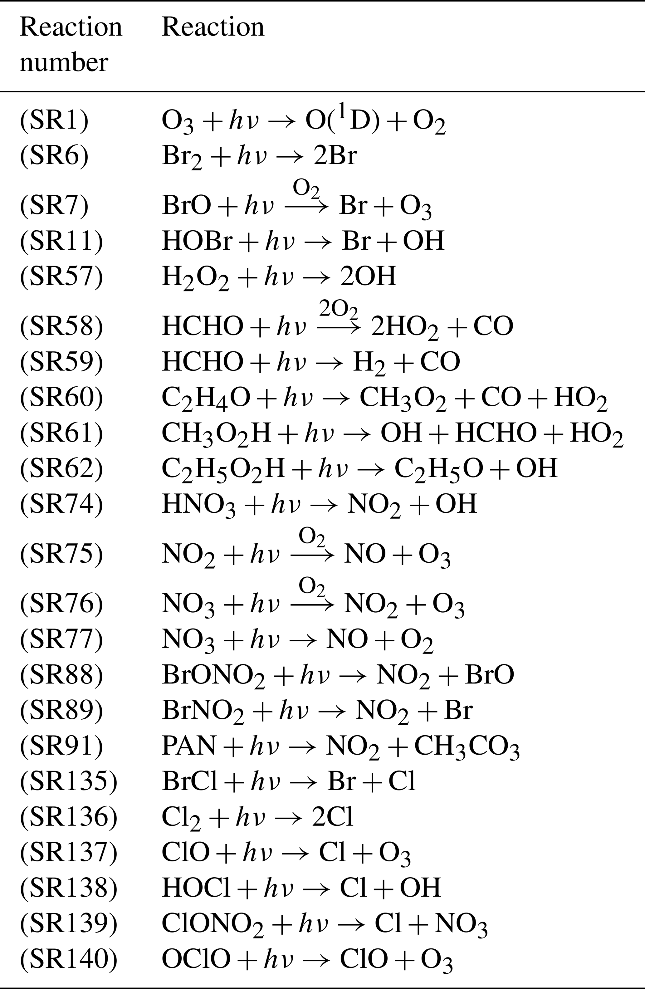
Table 2Initial atmospheric composition in the boundary layer of the Antarctic (ppm = parts per million, ppb = parts per billion, ppt = parts per trillion) (Piot, 2007), and the prescribed intensities of emission fluxes from the ground surface (units: molec. cm−2 s−1) (Hutterli et al., 2004; Riedel et al., 2005; Jones et al., 2011), assumed in the model.

In the KINAL model, it is also assumed that bromide stored in the ice and snow-covered ground surface is inexhaustible. As a result, the rates of heterogeneous reactions such as , which are responsible for the bromine explosion, only depend on the availability of HOBr in the atmosphere in model calculations. The rates of these heterogeneous reactions, v, are estimated as
In Eq. (4), [HOBr] and [Br2] are the concentrations of HOBr and Br2 in the boundary layer, respectively. L is the boundary layer height, and vd is the dry deposition velocity of HOBr at the ice/snow surface. The estimation of vd depends on the values of three resistances (i.e., ra, rb and rc), which are associated with the wind speed and the roughness of the ground surface (Seinfeld and Pandis, 2006). The wind speed was assumed as 8 m s−1 (Beare et al., 2006), which is a typical wind speed in polar regions. In addition, the roughness of the ice/snow surface is set to 10−5 m (Stull, 1988), and the height of the polar boundary layer is assumed to be 200 m because the typical thickness of the boundary layer in polar regions is about 100–500 m (Simpson et al., 2007; Anderson and Neff, 2008). Details of the parameterization of the heterogeneous reactions can be found in previous publications (Lehrer et al., 2004; Cao et al., 2014, 2016b). Aside from this parameterization, we also assumed that the loss of chemical species caused by dry deposition is equivalent to the flux brought by the entrainment from the free atmosphere into the boundary layer, which is similar to the treatment of Michalowski et al. (2000). By doing that, in the absence of chemistry, the concentrations of chemical species are able to remain in the balance of the dry deposition and the entrainment. The initial atmospheric composition used in the model is listed in Table 2, which represents a typical air composition in the Antarctic (Piot, 2007). Constant emission fluxes from the ground surface were also prescribed in the model according to observations (Hutterli et al., 2004; Riedel et al., 2005; Jones et al., 2011), and the prescribed intensities of the emission fluxes are also presented in Table 2.
2.2.3 Concentration sensitivity analysis
After obtaining the temporal evolution of ozone and major bromine species, relative concentration sensitivities of these species to different photolysis reactions in the chemical mechanism were computed to reveal the dependence of these species on each photolysis reaction of the mechanism. The relative concentration sensitivity Sij is calculated by
which shows the importance of the j-th reaction for the concentration change in the i-th chemical species. In Eq. (5), i is the index of chemical species, and j is the index of chemical reactions in the mechanism. ci is the concentration of the i-th species, and kj is the rate constant of the j-th reaction. Sij, an element of the relative sensitivity matrix, indicates the change in the i-th species concentration resulted from a small perturbation in the j-th reaction rate. The evaluation of the concentration sensitivity is helpful for discovering the importance of specific reactions in the chemical mechanism for the concentration change of the focused species.
In the following section, the computational results are presented and discussed.
In this section, we first show the connection between TOCs detected at two monitoring stations (i.e., Halley station and FAD station) and the tropospheric ODE observed at the Halley station. Later, we present the computational results of ODEs for a time period of 29 September–8 October 2008 as an example to show the time series of ozone and major bromine compounds in the troposphere during ODEs. The depletion rate of tropospheric ozone and the temporal evolution of bromine species under different conditions are then displayed to indicate the influence caused by TOC on the ozone depletion and the bromine activation. Finally, a concentration sensitivity analysis was performed to see which photolysis reactions play important roles in the connection between TOC and the occurrence of ODEs.
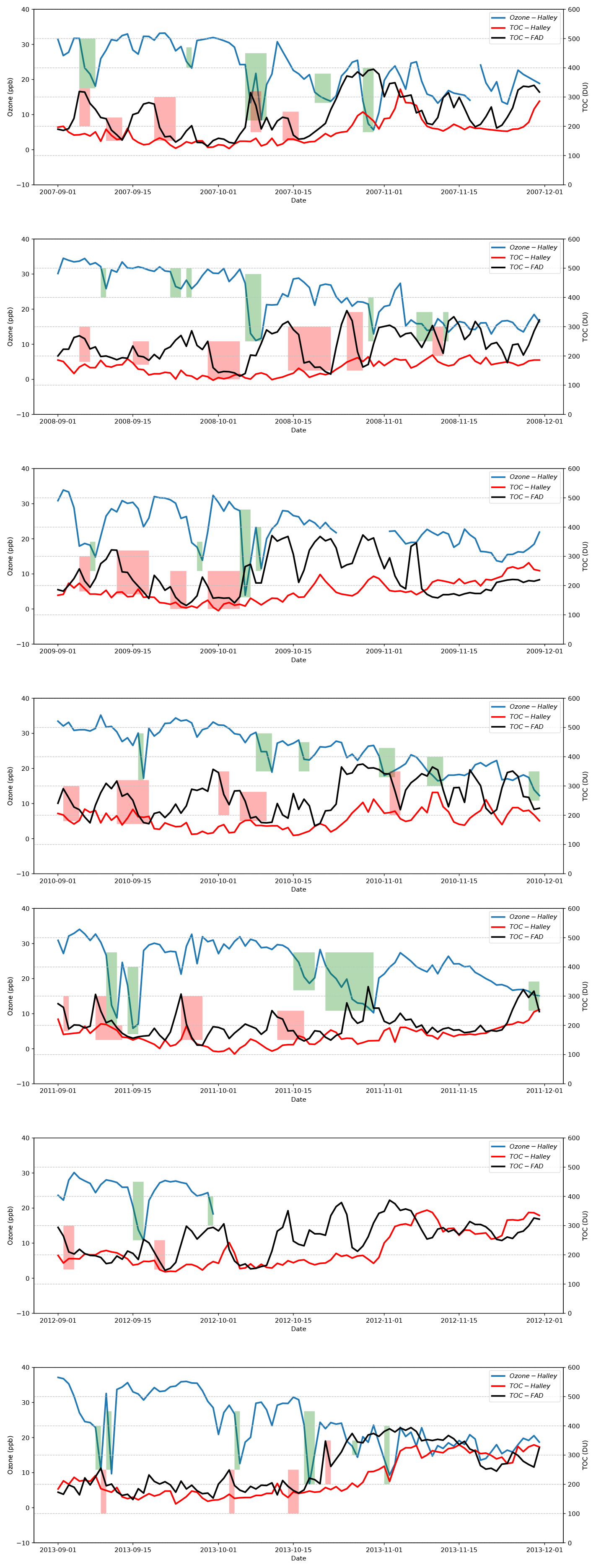
Figure 1Time series of TOCs belonging to the Halley station and the Faraday-Vernadsky (FAD) station as well as the surface ozone detected at the Halley station during the springtime of years 2007–2013 (the observational data of the surface ozone for October and November in the year 2012 are missing). The green-shaded areas in the figure indicate the periods identified as the occurrence of ODEs at Halley in the present study, and the red-shaded areas represent the significant decline in TOC at FAD, which might be associated with the occurrence of ODEs at Halley.
3.1 Relationship between the TOCs and the tropospheric ODE
The time series of the daily TOCs detected at the Halley station and the FAD station as well as the surface ozone of the Halley station during the springtime of years 2007–2013 are presented in Fig. 1. From the temporal evolution of the surface ozone, we found that at Halley, the occurrence frequency of ODEs in November is substantially lower than that in September or October. Moreover, by comparing the surface ozone of Halley with the TOC detected at Halley, we did not find any obvious correlation between them, except that the ODEs occurred more frequently in a relatively low TOC condition. However, from the comparison between the surface ozone of Halley and the TOC detected at the FAD station, we found that the ODEs observed at Halley usually followed a decline in TOC at the FAD station (see the shaded areas in Fig. 1). This suggests that the decrease of TOC surrounding FAD possibly favors the occurrence of ODEs at the Halley station. As the FAD station is located to the northwest of the Halley station and near the Weddell Sea, the TOC detected at this station is more capable of reflecting conditions of the Weddell Sea. Thus, we suggest that the possible mechanism is the decline in TOC over the area of the Weddell Sea that favors the tropospheric ozone depletion in this region. Then the ozone-lacking air was transported from the sea to the Halley station, leading to the detection of ODEs at this site. Thus, there exists a lag time between the TOC decline observed at the FAD station and the detection of ODEs at the Halley station, and the length of the lag time depends on the weather conditions during that period. In previous studies, the source of ODEs observed at Halley has also been discussed by Jones et al. (2006), who found that air masses causing rapid ODEs at Halley originated in the southern Weddell Sea. Our findings are consistent with the conclusions of Jones et al. (2006).
In order to further clarify the role of TOC in affecting the occurrence of ODEs, we then took the year 2008 as an example and used the models (i.e., TUV and KINAL) with the input of TOC observed at the FAD station. The reason we chose the year 2008 is that the TOC variation at the FAD station in this year is more stable than those in other years (see Fig. S2 in the Supplement).
3.2 Temporal behavior of tropospheric ozone and bromine species during ODEs in October 2008
The temporal profiles of tropospheric ozone and bromine species simulated by models implementing the daily variation of TOC observed at the FAD station from 29 September to 8 October 2008 are shown in Fig. 2. We chose this period because during this time a significant drop in TOC from 250 to 131 DU was observed at the FAD station (see Fig. S2 in the Supplement). From the temporal behavior of these chemical species, we can better understand the interconversion of bromine species and the reasons causing the depletion of ozone in the troposphere. Because similar results have been shown and discussed in previous publications (Cao et al., 2014, 2016a), we only briefly describe them here.

Figure 2Temporal profiles of tropospheric ozone and major bromine species during the ODE from 29 September to 8 October 2008.
It can be seen in Fig. 2 that the whole process of the ODE can be divided into four time stages, according to the types of bromine species in the troposphere. The first stage is the beginning of ODEs, in which the concentration of bromine is low, and ozone is only slightly depleted. This time stage would last for about 5 d in the present simulation (see Fig. 2). Subsequently, in the second time stage, Br2 released from substrates, such as the ice and snow-covered surface due to the bromine explosion mechanism is continuously photolyzed, forming Br atoms. The Br atoms then react with ozone and form BrO:
A part of BrO then becomes oxidized and converted to HOBr:
Thus, in the second time stage, the major bromine species are BrO and HOBr. In contrast, the concentration of Br is almost zero due to the presence of ozone. Under this high-HOBr environment a large amount of bromide is activated from substrates, so that ozone is rapidly consumed by the massive amount of bromine in the atmosphere. Thus, this second time stage is also the key time period that the majority of the tropospheric ozone is depleted, and this time stage lasts for about 1 d, in which the majority of ozone is depleted at a rate of 0.5–1.0 ppb h−1.
When the mixing ratio of ozone drops to less than 5 ppb, this event enters the third stage. In this time stage, the depletion of ozone continues, but the formation of BrO and HOBr are retarded, because of the low ozone in the atmosphere. The major bromine species at this time is Br, formed by the photodecomposition of BrO and HOBr in the atmosphere. Then the last stage comes, in which ozone in the troposphere is almost completely consumed. At this time stage, BrO and HOBr are all photolyzed to Br, and therefore do not exist in the atmosphere. Meanwhile, the Br formed is eliminated by aldehydes and HOx free radicals in the atmosphere, and is converted into HBr. As a result, at this last stage, a complete depletion of ozone in the troposphere is achieved, and the major bromine species is HBr, which is in accordance with previous observations (Langendörfer et al., 1999).
3.3 Impact of TOC on the occurrence of ODEs
We then compared the model results for different months of the springtime of 2008. The adopted time periods representing the 3 months for the present investigation are 1–10 September, 29 September–8 October and 1–10 November. The TOC variations in these three months can be found in Fig. S2 in the Supplement. However, it should be noted that aside from the difference in TOC, the value of the solar zenith angle (SZA) also varies between these months, which may significantly affect the radiation fluxes reaching the boundary layer and thus the rates of photolysis reactions.
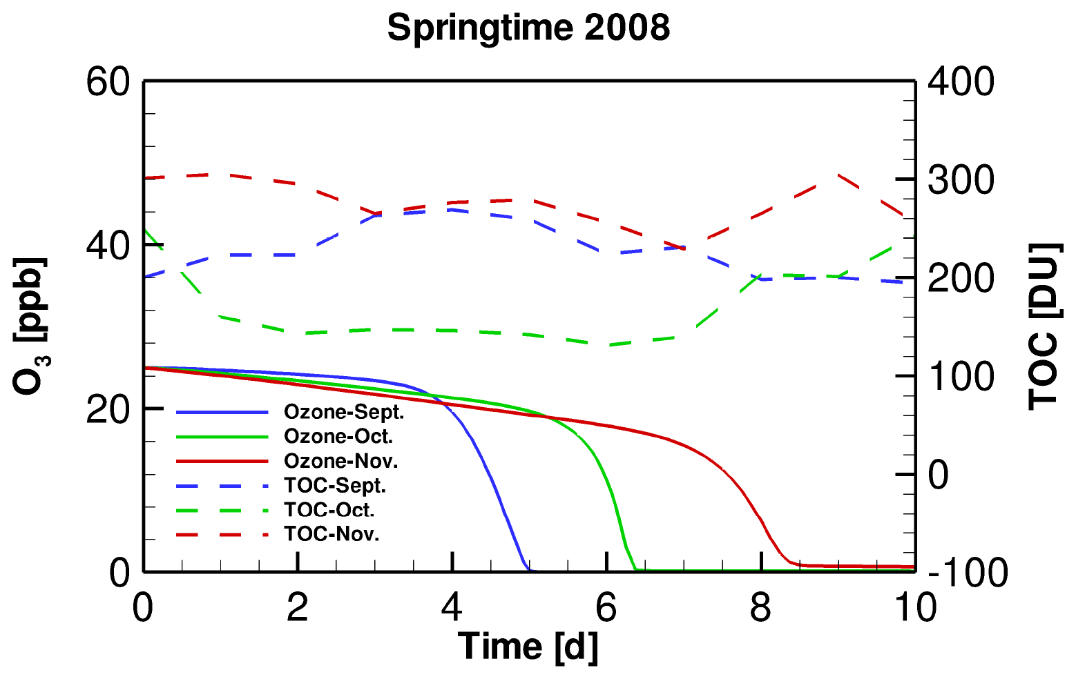
Figure 3Temporal profiles of TOC in different months of the springtime of 2008 and the simulated surface ozone during ODEs.
The temporal profiles of tropospheric ozone during ODEs under the conditions of different months of 2008 are shown in Fig. 3. It is seen that compared with the situation in September, the decline of ozone in November is delayed. Moreover, the depletion rate in November was also found to be lower than that in September. It suggests that under the weather conditions of November 2008, the occurrence of ODEs is more difficult to achieve, compared with that in September 2008. This result is also consistent with the relatively lower occurrence frequency of ODEs observed in November shown above. However, as mentioned above, although TOC differs between these months, it does not guarantee that the difference in the ODE occurrence between these simulations is caused by the use of different TOCs, because the SZA also varies, which may heavily influence the radiation fluxes reaching the ground surface and thus the occurrence frequency of ODEs. Therefore, we designed two sensitivity tests in the present study, to discover the role of SZA and TOC in affecting the ODEs separately.
In order to clarify the role of SZA in determining the occurrence of ODEs, we designed a sensitivity test by replacing the input TOC variation in September and November simulations with that belonging to October. By performing this test, we were able to discover the influence on the occurrence of ODEs solely by SZA. Figure 4 shows the temporal evolution of the surface ozone in this sensitivity test. It can be seen that when applying a same TOC variation in these simulations, the ozone depletion in September occurs remarkably earlier than that in November. It denotes that the decline of SZA leads to a retardation of ODEs. Thus, the ozone depletion is more difficult to achieve when SZA becomes smaller. The reasons for this positive association between SZA and the occurrence frequency of ODEs will be discussed in a later context.
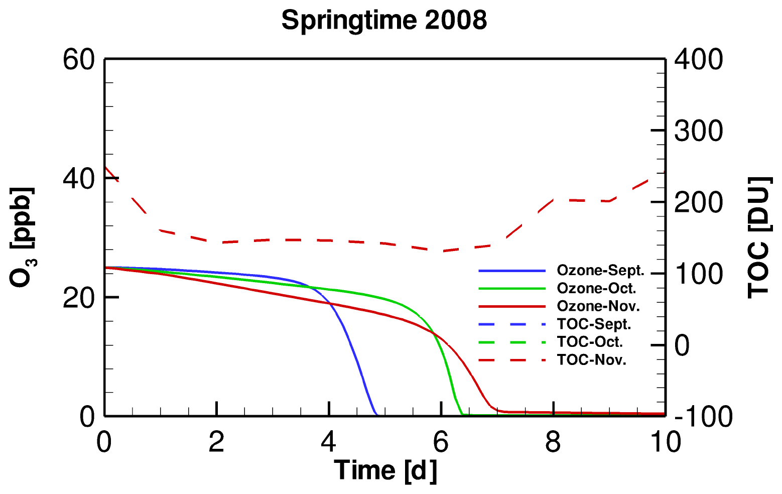
Figure 4Temporal evolution of tropospheric ozone during ODEs in different months of the springtime of 2008, using a same TOC temporal profile. Note that in this figure, the TOC profiles belonging to September, October and November overlap, because they are identical in this sensitivity test.
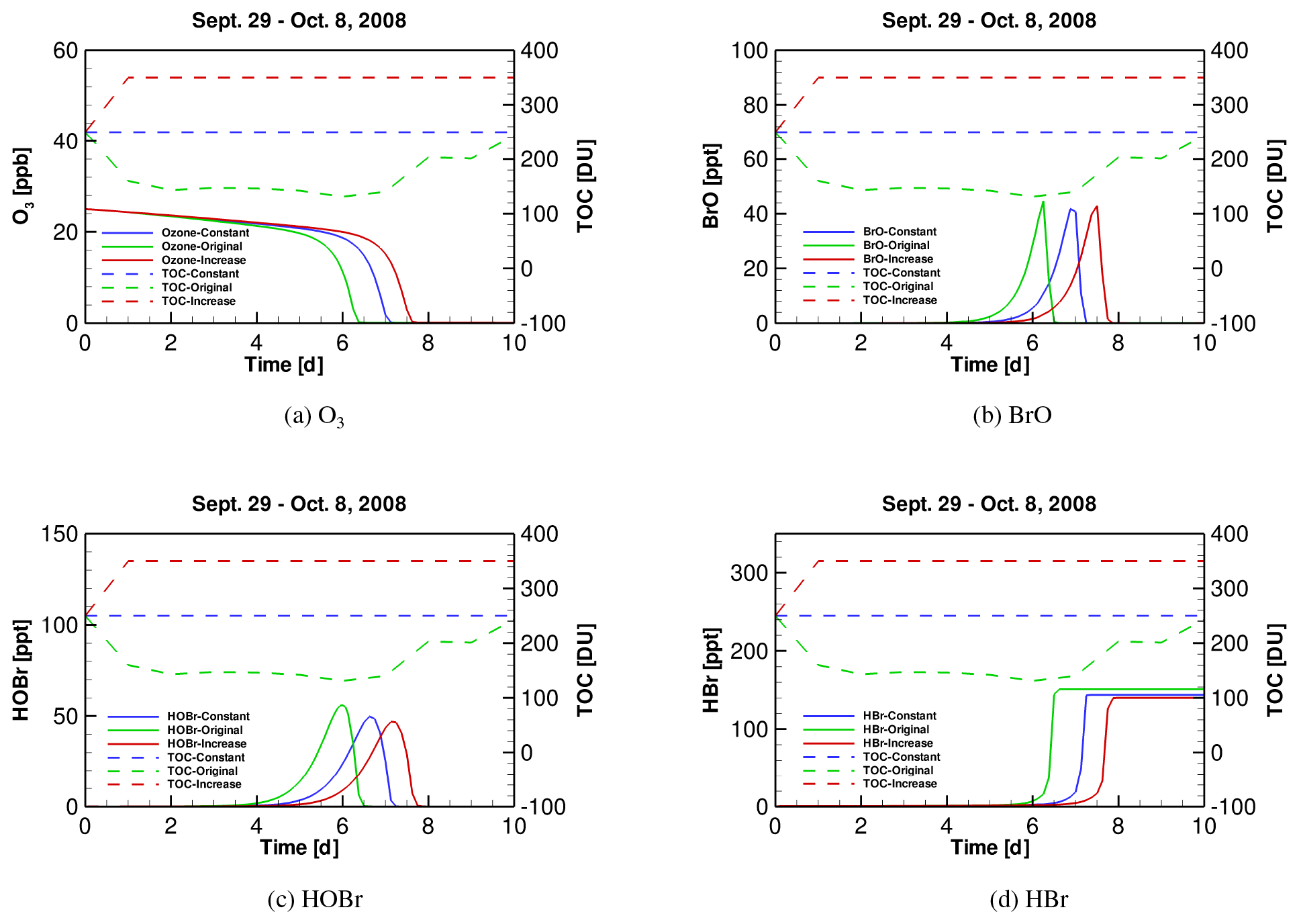
Figure 5Time series of (a) tropospheric ozone, (b) BrO, (c) HOBr and (d) HBr during ODEs under the conditions of October 2008, implementing three different TOC profiles (i.e., original, “constant” and “increase”).
After clarifying the role of SZA, we continued to discover the role of TOC in affecting ODEs. We thus implemented different temporal profiles of TOC in the October simulation. As mentioned above, in October TOC at the FAD station drops sharply from 250 DU on 29 September to 131 DU on 4 October. In this sensitivity test, we first assumed that the TOC keeps as a constant 250 DU instead of dropping, and we named this simulation scenario as the “constant” scenario. Next, we performed another simulation in which the TOC increases sharply from 250 to 350 DU from the beginning of the simulation rather than decreasing, and this scenario was named as “increase” in the following context. Thus, in these simulation scenarios, the TOC level in the original scenario is the lowest, while the TOC level in the “increase” scenario is the highest. In contrast, the values of SZA and other meteorological parameters are similar in these scenarios. By doing this, we were able to find out the impact on the occurrence of ODEs exerted by only TOC using TUV and KINAL models.
The temporal profiles of tropospheric ozone and major bromine species are presented in Fig. 5. It can be seen in Fig. 5a that when TOC in October is lower (i.e., the situation in the original simulation), the depletion of ozone is accelerated and the depletion rate becomes higher than those in the other two scenarios. It denotes that it takes less time for the ozone to be completely depleted under a lower TOC. Moreover, it can be found from Fig. 5b–d that the peaks of BrO, HOBr and HBr in the original simulation scenario occur earlier than those in the other two scenarios. In addition, it can be seen from Fig. 5d that the total amount of bromine in the atmosphere (i.e., in the form of HBr) at the end of ODEs in the original scenario is slightly higher than those in the other two scenarios. Thus, from the model results, the decrease of TOC enhances the occurrence of the tropospheric ODEs and the bromine release. This simulation result also partly supports our previous suggestion that the decline in TOC possibly favors the tropospheric ozone depletion in the analysis of the observational data.
The mechanism we proposed is that when TOC decreases, a larger amount of solar radiation would reach the troposphere, leading to an acceleration of a part of photochemical reactions associated with the ozone depletion and the bromine activation in the troposphere. As a result, the formation of major bromine species, such as BrO and HOBr as well as the bromine activation become faster, and the occurrence of ODEs is also accelerated.
However, it is still unclear through which photolysis reactions the variation of TOC deeply affects the occurrence of tropospheric ODEs. Thus, we continued to analyze the photochemical reactions using the concentration sensitivity analysis, as presented below.
3.4 Sensitivities of tropospheric ozone and major bromine species to photolysis reactions
In the present study, the impact on ODEs caused by TOC in the models is exerted through 23 photolysis reactions, which are listed in Table 1. In order to discover which photolysis reactions are the most important ones during the ODE process, we performed a concentration sensitivity analysis on tropospheric ozone and major bromine species for the simulation of October 2008 (i.e., the simulation presented in Sect. 3.2), so that the dependence of tropospheric ozone and bromine species on these photolysis reactions can be revealed.
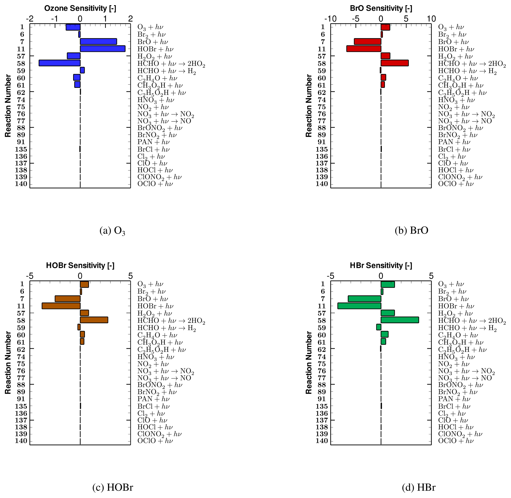
Figure 6Relative sensitivities of (a) tropospheric ozone, (b) BrO, (c) HOBr and (d) HBr to photolysis reactions on day 5.8, which resides in the time period when the strongest ozone depletion occurs.
The relative concentration sensitivities of tropospheric ozone and major bromine species (i.e., BrO, HOBr and HBr) to all the 23 photolysis reactions on day 5.8, which resides in the second time stage of ODEs when the strongest ozone depletion occurs (see Fig. 2), are shown in Fig. 6. From Fig. 6a, it can be seen that reactions (SR7) and (SR11):
possess the largest positive sensitivities for the mixing ratio of ozone. It means that the rate increase of these two photolysis reactions leads to an elevation of the ozone value during ODEs and thus a retardation of ODEs. These two reactions are thus named “major ODE decelerating reactions” in the following context. The reason for the delayed impact on ODEs brought by reaction (SR7) is that in this reaction, BrO is photolyzed, forming Br. As a result, the formation of HOBr by the oxidation of BrO is decelerated due to the reduction of the available BrO. Thus, the heterogeneous bromine activation process, i.e., bromine explosion mechanism that HOBr participates in, is retarded, leading to a slowing down of the bromine activation and the ozone depletion. Apart from that, additional ozone is also formed through reaction (SR7). With respect to reaction (SR11), HOBr is photodecomposed through this reaction. Thus, the heterogeneous bromine activation also gets suppressed by the strengthening of this reaction, resulting in a delay of the ozone depletion.
In contrast, reactions (SR1), (SR57), and (SR58),
are largely negatively correlated with the change in ozone (see Fig. 6a). It denotes that when these three reactions speed up, the level of ozone drops, which represents an acceleration of the tropospheric ODE. These three reactions are thus named “major ODE accelerating reactions”. For reaction (SR1), it is not surprising as this reaction is the direct photolysis of the tropospheric ozone. Moreover, reaction (SR1) also serves as a major formation pathway of OH radicals. OH radicals are important for the occurrence of ODEs and the bromine explosion mechanism, as they are involved in reaction (SR18):
In reaction (SR18), not only the Br atoms are generated by the conversion from the released Br2, but also the formation of HOBr is strengthened, leading to an acceleration of the bromine activation. As a result, an enhancement of reaction (SR1) would lead to a speeding up of the ozone depletion. Regarding reaction (SR57), the occurrence of this reaction also strengthens the occurrence of ODEs, because this reaction also forms OH radicals, which are critical for the bromine explosion mechanism as mentioned above. With respect to reaction (SR58), it possesses the most negative ozone sensitivity (see Fig. 6a), which means that this reaction heavily controls the depletion of ozone. This is because this reaction reinforces the formation of HO2. As HO2 is the key oxidant for the formation of HOBr through reaction:
the enhancement of reaction (SR58) thus favors the release of bromine and the depletion of ozone.
From Fig. 6b–d, it can be seen that the sensitivities of major bromine species (i.e., BrO, HOBr and HBr) to photolysis reactions mostly have an opposite sign, compared with those corresponding to ozone (shown in Fig. 6a). This is because the bromine species in the atmosphere are mostly responsible for the ozone depletion in the troposphere during ODEs. Within these photolysis reactions, reactions (SR7) and (SR11) have the largest negative sensitivities as they strongly decelerate the bromine explosion mechanism. In contrast, reactions (SR1), (SR57) and (SR58) exert a positive impact on the change in bromine species. This is because the speeding up of these three reactions can reinforce the bromine explosion mechanism as mentioned above, thus leading to a positive dependence of these bromine-containing compounds on these three reactions.
The results of the sensitivity analysis help to explain the impact on the occurrence of ODEs exerted by SZA in previous discussions. First, in the comparison of the simulation results corresponding to different months of 2008 (see Figs. 3 and 4 in Sect. 3.3), it was found that the tropospheric ODE is more difficult to achieve in November than in September due to a smaller SZA in November. From the sensitivity analysis, we were able to discover the reason for the retardation of ODEs caused by the smaller SZA. Due to the shift in SZA, solar radiation with all the wavelengths that reach the ground surface is strengthened in November. Consequently, although the TOC value in November is higher than that in September, both the major ODE accelerating reactions (i.e., reactions SR1, SR57 and SR58) and the major ODE decelerating reactions (i.e., reactions SR7 and SR11) are promoted in November. From Fig. 6a, it can be seen that the ozone level during ODEs is more sensitive to the major ODE decelerating reactions than the major ODE accelerating reactions. As a result, the outcome of the SZA decline in November is that the occurrence of ODEs is retarded. In this situation, TOC only plays a minor role in affecting the occurrence of ODEs.
In contrast, in the comparison of the ODE occurrence belonging to October using different TOC profiles (see Fig. 5 in Sect. 3.3), because the values of the SZA are similar in these scenarios, the change in ODEs is mainly determined by the difference in TOC between these simulations. In a lower TOC environment, the intensity of the solar radiation reaching the atmospheric boundary layer, especially the ultraviolet radiation in a wavelength range of 200–320 nm (i.e., UV-B and UV-C), is significantly enhanced, as ozone has strong absorption bands in 200–320 nm (i.e., Hartley bands). Moreover, solar radiation in 320–350 nm also becomes moderately elevated under a low TOC condition, because of the absorption bands of ozone in 320–350 nm with a vibrational structure (i.e., Huggins bands). On the contrary, solar radiation in other wavelength ranges would not be significantly affected by the decrease of TOC. In this situation, the major ODE accelerating reactions, i.e., photolysis of ozone, H2O2 and HCHO in the boundary layer, are remarkably promoted. The reasons are as follows: (1) the photolysis of ozone in the troposphere that forms O(1D) depends heavily on the strength of the solar radiation in 295–360 nm (Akimoto, 2016). Thus, the decrease in TOC would significantly accelerate the photolysis of ozone in the troposphere, i.e., reaction (SR1). (2) The absorption cross-section of H2O2 decreases monotonically from the wavelength of 190 to 350 nm (Vaghjiani and Ravishankara, 1989), which overlaps the wavelength range that the TOC change strongly affects. Thus, the photodecomposition of H2O2 (i.e., reaction SR57) also becomes strongly promoted when TOC decreases. (3) The absorption spectrum of HCHO spreads from 260 to 360 nm, with many vibrational structures (Rogers, 1990). As a result, the decline of TOC substantially enhances the photolysis of HCHO (i.e., reaction SR58).
On the contrary, for the major ODE decelerating reactions, i.e., photolysis of BrO and HOBr, the rates are only slightly influenced by the decrease of TOC. This is because BrO has an absorption spectrum in the range of 290–380 nm, peaking at approximately 330 nm (Wilmouth et al., 1999). The strengthening of the solar radiation especially in 200–320 nm due to the decline of TOC thus only exerts a small influence on the photolysis of BrO (i.e., reaction SR7). Regarding HOBr, its photolysis rate relies more on the strength of the UV-A radiation (i.e., in 320–400 nm) reaching the boundary layer, as it has a broad absorption spectrum between 200 and 400 nm (Burkholder et al., 2015). Therefore, the influence caused by TOC on the photolysis of HOBr is also weak.
Hence, it can be concluded that when TOC decreases, the rates of major ODE accelerating reactions (i.e., reactions SR1, SR57 and SR58) significantly increase, while the rates of major ODE decelerating reactions (i.e., reactions SR7 and SR11) are hardly changed. Consequently, the ODEs are accelerated under a low TOC condition, and vice versa, resulting in a negative association between TOC and the occurrence frequency of ODEs as presented above.
In this study, we investigated the connection between the total ozone column (TOC) and the occurrence of the tropospheric ozone depletion events (ODEs) in the Antarctic. Photolysis reactions dominating this connection were also identified using a concentration sensitivity analysis. Major conclusions achieved in the present study are as follows.
Based on the analysis of the observational data from the years 2007–2013, we suggested that the decrease of TOC surrounding the Faraday-Vernadsky (FAD) station possibly favors the occurrence of the tropospheric ODEs at the Halley station. Then, the model results with the implementation of different TOC profiles also indicate that the occurrence of ODEs would be accelerated when TOC decreases. Moreover, key photolysis reactions that dominate the production and the consumption of tropospheric ozone during ODEs, i.e., major ODE accelerating reactions and major ODE decelerating reactions, were also discovered. It was found that when TOC varies, the rates of major ODE accelerating reactions are substantially altered, while the rates of major ODE decelerating reactions mostly remain unchanged, leading to the negative association between TOC and the occurrence frequency of ODEs.
Improvements can be made to the present study. For instance, many other factors that are able to influence the occurrence of ODEs, such as the type of sea ice and the existence of frost flowers, should be considered in future work. Unfortunately, currently we still lack these observational data. Apart from that, a study for Arctic conditions should also be conducted, so that the conclusions obtained in the present study can be compared and verified, which will be covered in a future publication.
The observational data used in this study and the source code of the models as well as the computational results shown in this article can be acquired from the link https://faculty.nuist.edu.cn/caole/en/kyxm/72647/content/17580.htm#kyxm (Cao, 2022).
The supplement related to this article is available online at: https://doi.org/10.5194/acp-22-3875-2022-supplement.
LC conceived the idea of the article and extended the KINAL model. LF processed the observational data, performed the computations, and wrote the paper together with LC. SL revised the chemical mechanisms and SY gave valuable suggestions on the improvement of the manuscript. All the authors listed have read and approved the final manuscript.
The contact author has declared that neither they nor their co-authors have any competing interests.
Publisher’s note: Copernicus Publications remains neutral with regard to jurisdictional claims in published maps and institutional affiliations.
The numerical calculations in this paper have been done on the high performance computing system in the High Performance Computing Center, Nanjing University of Information Science and Technology.
This research has been supported by the National Natural Science Foundation of China (grant no. 41705103).
This paper was edited by Marc von Hobe and reviewed by two anonymous referees.
Akimoto, H.: Atmospheric Reaction Chemistry, in: Springer Atmospheric Sciences, edition no. 1, Springer, Japan, https://doi.org/10.1007/978-4-431-55870-5, 2016. a, b
Anderson, P. S. and Neff, W. D.: Boundary layer physics over snow and ice, Atmos. Chem. Phys., 8, 3563–3582, https://doi.org/10.5194/acp-8-3563-2008, 2008. a
Atkinson, R., Baulch, D. L., Cox, R. A., Crowley, J. N., Hampson, R. F., Hynes, R. G., Jenkin, M. E., Rossi, M. J., Troe, J., and IUPAC Subcommittee: Evaluated kinetic and photochemical data for atmospheric chemistry: Volume II – gas phase reactions of organic species, Atmos. Chem. Phys., 6, 3625–4055, https://doi.org/10.5194/acp-6-3625-2006, 2006. a
Balis, D., Kroon, M., Koukouli, M. E., Brinksma, E. J., Labow, G., Veefkind, J. P., and McPeters, R. D.: Validation of Ozone Monitoring Instrument total ozone column measurements using Brewer and Dobson spectrophotometer ground-based observations, J. Geophys. Res.-Atmos., 112, D24S46, https://doi.org/10.1029/2007JD008796, 2007. a
Beare, R., Macvean, M., Holtslag, A., Cuxart, J., Esau, I., Golaz, J.-C., Jimenez, M., Khairoutdinov, M., Kosovic, B., Lewellen, D., Lund, T., Lundquist, J., Mccabe, A., Moene, A., Noh, Y., Raasch, S., and Sullivan, P.: An intercomparison of large-eddy simulations of the stable boundary layer, Boundary Layer Meteorol., 118, 247–272, https://doi.org/10.1007/s10546-004-2820-6, 2006. a
Bedjanian, Y. and Poulet, G.: Kinetics of Halogen Oxide Radicals in the Stratosphere, Chem. Rev., 103, 4639–4656, https://doi.org/10.1021/cr0205210, pMID: 14664627, 2003. a
Bian, L., Ye, L., Ding, M., Gao, Z., Zheng, X., and Schnell, R.: Surface Ozone Monitoring and Background Concentration at Zhongshan Station, Antarctica, Atmospheric and Climate Sciences, 8, 1–14, https://doi.org/10.4236/acs.2018.81001, 2018. a, b
Bottenheim, J. W. and Chan, E.: A trajectory study into the origin of spring time Arctic boundary layer ozone depletion, J. Geophys. Res.-Atmos., 111, D19301, https://doi.org/10.1029/2006JD007055, 2006. a
Bottenheim, J. W., Netcheva, S., Morin, S., and Nghiem, S. V.: Ozone in the boundary layer air over the Arctic Ocean: measurements during the TARA transpolar drift 2006–2008, Atmos. Chem. Phys., 9, 4545–4557, https://doi.org/10.5194/acp-9-4545-2009, 2009. a, b, c
Boylan, P., Helmig, D., Staebler, R., Turnipseed, A., Fairall, C., and Neff, W.: Boundary layer dynamics during the Ocean-Atmosphere-Sea-Ice-Snow (OASIS) 2009 experiment at Barrow, AK, J. Geophys. Res.-Atmos., 119, 2261–2278, https://doi.org/10.1002/2013JD020299, 2014. a
Brasseur, G. and Solomon, S.: Aeronomy of the Middle Atmosphere: Chemistry and Physics of the Stratosphere and Mesosphere, Edition no. 3, Springer, https://doi.org/10.1007/1-4020-3824-0, 2005. a
Burkholder, J., Sander, S., Abbatt, J., Barker, J., Huie, R., Kolb, C., Kurylo, M., Orkin, V., Wilmouth, D., and Wine, P.: Chemical Kinetics and Photochemical Data for Use in Atmospheric Studies, Evaluation Number 18, Tech. rep., JPL Publication 15-10, Jet Propulsion Laboratory, Pasadena, https://doi.org/10.13140/RG.2.1.2504.2806, 2015. a
Cao, L.: The observational data and the source code of the models as well as the computational results for “Influence of Total Ozone Column (TOC) on the Occurrence of Tropospheric Ozone Depletion Events (ODEs) in the Antarctic”, NUIST Information Platform [code and data set], https://faculty.nuist.edu.cn/caole/en/kyxm/72647/content/17580.htm#kyxm, last access: 14 February 2022. a
Cao, L., Sihler, H., Platt, U., and Gutheil, E.: Numerical analysis of the chemical kinetic mechanisms of ozone depletion and halogen release in the polar troposphere, Atmos. Chem. Phys., 14, 3771–3787, https://doi.org/10.5194/acp-14-3771-2014, 2014. a, b, c
Cao, L., He, M., Jiang, H., Grosshans, H., and Cao, N.: Sensitivity of the Reaction Mechanism of the Ozone Depletion Events during the Arctic Spring on the Initial Atmospheric Composition of the Troposphere, Atmosphere, 7, 124, https://doi.org/10.3390/atmos7100124, 2016a. a, b
Cao, L., Platt, U., and Gutheil, E.: Role of the boundary layer in the occurrence and termination of the tropospheric ozone depletion events in polar spring, Atmos. Environ., 132, 98–110, https://doi.org/10.1016/j.atmosenv.2016.02.034, 2016b. a
Cao, L., Wang, C., Mao, M., Grosshans, H., and Cao, N.: Derivation of the reduced reaction mechanisms of ozone depletion events in the Arctic spring by using concentration sensitivity analysis and principal component analysis, Atmos. Chem. Phys., 16, 14853–14873, https://doi.org/10.5194/acp-16-14853-2016, 2016c. a
Farman, J. C., Gardiner, B. G., and Shanklin, J. D.: Large losses of total ozone in Antarctica reveal seasonal ClOx NOx interaction, Nature, 315, 207–210, https://doi.org/10.1038/315207a0, 1985. a
Finlayson-Pitts, B. and Pitts, J.: Chemistry of the Upper and Lower Atmosphere: Theory, Experiments and Applications, Edition no. 1, Academic Press, San Deigo, https://doi.org/10.1016/B978-0-12-257060-5.X5000-X, 1999. a
Fishman, J. and Crutzen, P. J.: The origin of ozone in the troposphere, Nature, 274, 855–858, 1978. a
Frieß, U., Hollwedel, J., König-Langlo, G., Wagner, T., and Platt, U.: Dynamics and chemistry of tropospheric bromine explosion events in the Antarctic coastal region, J. Geophys. Res., 109, D06305, https://doi.org/10.1029/2003JD004133, 2004. a
Heinemann, G.: The polar regions: a natural laboratory for boundary layer meteorology a review, Meteorologische Z., 17, 589–601, https://doi.org/10.1127/0941-2948/2008/0327, 2008. a
Hopper, J. F., Barrie, L. A., Silis, A., Hart, W., Gallant, A. J., and Dryfhout, H.: Ozone and meteorology during the 1994 Polar Sunrise Experiment, J. Geophys. Res., 103, 1481–1492, https://doi.org/10.1029/97JD02888, 1998. a
Hu, X.-M., Zhang, F., Yu, G., Fuentes, J. D., and Wu, L.: Contribution of mixed-phase boundary layer clouds to the termination of ozone depletion events in the Arctic, Geophys. Res. Lett., 38, L21801, https://doi.org/10.1029/2011GL049229, 2011. a
Hutterli, M. A., McConnell, J. R., Chen, G., Bales, R. C., Davis, D. D., and Lenschow, D. H.: Formaldehyde and hydrogen peroxide in air, snow and interstitial air at South Pole, Atmos. Environ., 38, 5439–5450, https://doi.org/10.1016/j.atmosenv.2004.06.003, 2004. a, b
Jacobi, H.-W., Kaleschke, L., Richter, A., Rozanov, A., and Burrows, J. P.: Observation of a fast ozone loss in the marginal ice zone of the Arctic Ocean, J. Geophys. Res.-Atmos., 111, D15309, https://doi.org/10.1029/2005JD006715, 2006. a
Jacobi, H.-W., Morin, S., and Bottenheim, J. W.: Observation of widespread depletion of ozone in the springtime boundary layer of the central Arctic linked to mesoscale synoptic conditions, J. Geophys. Res., 115, D17302, https://doi.org/10.1029/2010JD013940, 2010. a
Jones, A. E., Anderson, P. S., Wolff, E. W., Turner, J., Rankin, A. M., and Colwell, S. R.: A role for newly forming sea ice in springtime polar tropospheric ozone loss? Observational evidence from Halley station, Antarctica, J. Geophys. Res.-Atmos., 111, D08306, https://doi.org/10.1029/2005JD006566, 2006. a, b, c, d
Jones, A. E., Wolff, E. W., Ames, D., Bauguitte, S. J.-B., Clemitshaw, K. C., Fleming, Z., Mills, G. P., Saiz-Lopez, A., Salmon, R. A., Sturges, W. T., and Worton, D. R.: The multi-seasonal NOy budget in coastal Antarctica and its link with surface snow and ice core nitrate: results from the CHABLIS campaign, Atmos. Chem. Phys., 11, 9271–9285, https://doi.org/10.5194/acp-11-9271-2011, 2011. a, b
Kaleschke, L., Richter, A., Burrows, J., Afe, O., Heygster, G., Notholt, J., Rankin, A. M., Roscoe, H. K., Hollwedel, J., Wagner, T., and Jacobi, H.-W.: Frost flowers on sea ice as a source of sea salt and their influence on tropospheric halogen chemistry, Geophys. Res. Lett., 31, L16114, https://doi.org/10.1029/2004GL020655, 2004. a
Koo, J.-H., Wang, Y., Kurosu, T. P., Chance, K., Rozanov, A., Richter, A., Oltmans, S. J., Thompson, A. M., Hair, J. W., Fenn, M. A., Weinheimer, A. J., Ryerson, T. B., Solberg, S., Huey, L. G., Liao, J., Dibb, J. E., Neuman, J. A., Nowak, J. B., Pierce, R. B., Natarajan, M., and Al-Saadi, J.: Characteristics of tropospheric ozone depletion events in the Arctic spring: analysis of the ARCTAS, ARCPAC, and ARCIONS measurements and satellite BrO observations, Atmos. Chem. Phys., 12, 9909–9922, https://doi.org/10.5194/acp-12-9909-2012, 2012. a, b
Koo, J.-H., Wang, Y., Jiang, T., Deng, Y., Oltmans, S. J., and Solberg, S.: Influence of climate variability on near-surface ozone depletion events in the Arctic spring, Geophys. Res. Lett., 41, 2582–2589, https://doi.org/10.1002/2014GL059275, 2014. a
Kreher, K., Johnston, P. V., Wood, S. W., Nardi, B., and Platt, U.: Ground-based measurements of tropospheric and stratospheric BrO at Arrival Heights, Antarctica, Geophys. Res. Lett., 24, 3021–3024, https://doi.org/10.1029/97GL02997, 1997. a
Krueger, A. J. and Minzner, R. A.: A mid-latitude ozone model for the 1976 U.S. Standard Atmosphere, J. Geophys. Res., 81, 4477–4481, https://doi.org/10.1029/JC081i024p04477, 1976. a
Kumar, P., Kuttippurath, J., Gathen, P., Petropavlovskikh, I., Johnson, B., McClure-Begley, A., Cristofanelli, P., Bonasoni, P., Barlasina, M., and Sánchez, R.: The Increasing Surface Ozone and Tropospheric Ozone in Antarctica and Their Possible Drivers, Environ. Sci. Technol., 55, 8542–8553, https://doi.org/10.1021/acs.est.0c08491, 2021. a
Kuttippurath, J., Goutail, F., Pommereau, J.-P., Lefèvre, F., Roscoe, H. K., Pazmiño, A., Feng, W., Chipperfield, M. P., and Godin-Beekmann, S.: Estimation of Antarctic ozone loss from ground-based total column measurements, Atmos. Chem. Phys., 10, 6569–6581, https://doi.org/10.5194/acp-10-6569-2010, 2010. a
Langendörfer, U., Lehrer, E., Wagenbach, D., and Platt, U.: Observation of filterable bromine variabilities during Arctic tropospheric ozone depletion events in high (1 h) time resolution, J. Atmos. Chem., 34, 39–54, https://doi.org/10.1023/A:1006217001008, 1999. a
Lehrer, E., Hönninger, G., and Platt, U.: A one dimensional model study of the mechanism of halogen liberation and vertical transport in the polar troposphere, Atmos. Chem. Phys., 4, 2427–2440, https://doi.org/10.5194/acp-4-2427-2004, 2004. a, b
Lippmann, M.: Health effects of tropospheric ozone, Environ. Sci. Technol., 25, 1954–1962, https://doi.org/10.1021/es00024a001, 1991. a
Madronich, S. and Flocke, S.: Theoretical Estimation of Biologically Effective UV Radiation at the Earth's Surface, in: Solar Ultraviolet Radiation, NATO ASI Series, vol. 52, edited by: Zerefos, C. S. and Bais, A. F., Springer, Berlin, Heidelberg, 23–48, https://doi.org/10.1007/978-3-662-03375-3_3, 1997. a, b
Madronich, S. and Flocke, S.: The Role of Solar Radiation in Atmospheric Chemistry, in: Environmental Photochemistry. The Handbook of Environmental Chemistry, vol. 2/2L, edited by: Boule, P., Springer, Berlin, Heidelberg, 1–26, https://doi.org/10.1007/978-3-540-69044-3_1, 1999. a, b
Michalowski, B. A., Francisco, J. S., Li, S.-M., Barrie, L. A., Bottenheim, J. W., and Shepson, P. B.: A computer model study of multiphase chemistry in the Arctic boundary layer during polar sunrise, J. Geophys. Res.-Atmos., 105, 15131–15145, https://doi.org/10.1029/2000JD900004, 2000. a
Molina, M. J. and Rowland, F. S.: Stratospheric sink for chlorofluoromethanes: chlorine atom-catalysed destruction of ozone, Nature, 249, 810–812, 1974. a
Oltmans, S. J.: Surface ozone measurements in clean air, J. Geophys. Res., 86, 1174–1180, https://doi.org/10.1029/JC086iC02p01174, 1981. a
Piot, M.: Modeling Halogen Chemistry during Ozone Depletion Events in Polar Spring: A Model Study, PhD thesis, University of Heidelberg, Germany, https://doi.org/10.11588/heidok.00007876,, 2007. a, b
Platt, U. and Janssen, C.: Observation and role of the free radicals NO3, ClO, BrO and IO in the troposphere, Faraday Discuss., 100, 175–198, https://doi.org/10.1039/FD9950000175, 1995. a
Platt, U. and Lehrer, E.: Arctic tropospheric ozone chemistry, ARCTOC, no. 64 in Air pollution research report, European Commission Directorate-General, Science, Research and Development, Luxembourg, ISBN 92-828-2350-4, 1997. a
Prather, M. and Jaffe, A. H.: Global impact of the Antarctic ozone hole: Chemical propagation, J. Geophys. Res.-Atmos., 95, 3473–3492, https://doi.org/10.1029/JD095iD04p03473, 1990. a
Riedel, K., Allan, W., Weller, R., and Schrems, O.: Discrepancies between formaldehyde measurements and methane oxidation model predictions in the Antarctic troposphere: An assessment of other possible formaldehyde sources, J. Geophys. Res.-Atmos., 110, D15308, https://doi.org/10.1029/2005JD005859, 2005. a, b
Rogers, J. D.: Ultraviolet absorption cross sections and atmospheric photodissociation rate constants of formaldehyde, J. Phys. Chem., 94, 4011–4015, https://doi.org/10.1021/j100373a025, 1990. a
Roscoe, H. K. and Roscoe, J.: Polar tropospheric ozone depletion events observed in the International Geophysical Year of 1958, Atmos. Chem. Phys., 6, 3303–3314, https://doi.org/10.5194/acp-6-3303-2006, 2006. a
Seinfeld, J. and Pandis, S.: Atmospheric chemistry and physics: from air pollution to climate change, 2nd Edn., Wiley-Intersciencie publications, Wiley, Hoboken, NJ, USA, ISBN 978-1-119-22117-3, 2006. a, b, c
Simpson, W. R., von Glasow, R., Riedel, K., Anderson, P., Ariya, P., Bottenheim, J., Burrows, J., Carpenter, L. J., Frieß, U., Goodsite, M. E., Heard, D., Hutterli, M., Jacobi, H.-W., Kaleschke, L., Neff, B., Plane, J., Platt, U., Richter, A., Roscoe, H., Sander, R., Shepson, P., Sodeau, J., Steffen, A., Wagner, T., and Wolff, E.: Halogens and their role in polar boundary-layer ozone depletion, Atmos. Chem. Phys., 7, 4375–4418, https://doi.org/10.5194/acp-7-4375-2007, 2007. a, b
Stull, R. B.: An Introduction to Boundary Layer Meteorology, Edition no. 1, Springer, Dordrecht, https://doi.org/10.1007/978-94-009-3027-8, 1988. a
Tarasick, D. W. and Bottenheim, J. W.: Surface ozone depletion episodes in the Arctic and Antarctic from historical ozonesonde records, Atmos. Chem. Phys., 2, 197–205, https://doi.org/10.5194/acp-2-197-2002, 2002. a, b
Turányi, T.: KINAL – a program package for kinetic analysis of reaction mechanisms, Comput. Chem., 14, 253–254, 1990. a, b, c
Vaghjiani, G. L. and Ravishankara, A. R.: Absorption cross sections of CH3OOH, H2O2, and D2O2 vapors between 210 and 365 nm at 297 K, J. Geophys. Res.-Atmos., 94, 3487–3492, https://doi.org/10.1029/JD094iD03p03487, 1989. a
van Oss, R. F. and Spurr, R. J.: Fast and accurate 4 and 6 stream linearized discrete ordinate radiative transfer models for ozone profile retrieval, J. Quant. Spectrosc Ra., 75, 177–220, https://doi.org/10.1016/S0022-4073(01)00246-1, 2002. a
Wagner, T., Ibrahim, O., Sinreich, R., Frieß, U., von Glasow, R., and Platt, U.: Enhanced tropospheric BrO over Antarctic sea ice in mid winter observed by MAX-DOAS on board the research vessel Polarstern, Atmos. Chem. Phys., 7, 3129–3142, https://doi.org/10.5194/acp-7-3129-2007, 2007. a
Wennberg, P.: Atmospheric chemistry: Bromine explosion, Nature, 397, 299–301, https://doi.org/10.1038/16805, 1999. a
Wilmouth, D. M., Hanisco, T. F., Donahue, N. M., and Anderson, J. G.: Fourier Transform Ultraviolet Spectroscopy of the A Transition of BrO, J. Phys. Chem. A, 103, 8935–8945, https://doi.org/10.1021/jp991651o, 1999. a
Zhou, J., Cao, L., and Li, S.: Influence of the Background Nitrogen Oxides on the Tropospheric Ozone Depletion Events in the Arctic during Springtime, Atmosphere, 11, 344, https://doi.org/10.3390/atmos11040344, 2020. a