Characterization of transport from the Asian summer monsoon anticyclone into the UTLS via shedding of low potential vorticity cutoffs

Air mass transport within the summertime Asian monsoon circulation provides a major source of anthropogenic pollution for the upper troposphere and lower stratosphere (UTLS). Here, we investigate the quasi-horizontal transport of air masses from the Asian summer monsoon anticyclone (ASMA) into the extratropical lower stratosphere and their chemical evolution. For that reason, we developed a method to identify and track the air masses exported from the monsoon. This method is based on the anomalously low potential vorticity (PV) of these air masses (tropospheric low PV cutoffs) compared to the lower stratosphere and uses trajectory calculations and chemical fields from the Chemical Lagrangian Model of the Stratosphere (CLaMS). The results show evidence of frequent summertime transport from the monsoon anticyclone to midlatitudes over the North Pacific, even reaching the high-latitude regions of Siberia and Alaska. Most of the low PV cutoffs related to air masses exported from the ASMA have lifetimes shorter than 1 week (about 90 %) and sizes smaller than 1 % of the Northern Hemisphere (NH) area. The chemical composition of these air masses is characterized by carbon monoxide, ozone, and water vapour mixing ratios at an intermediate range between values typical for the monsoon anticyclone and the lower stratosphere. The chemical evolution during transport within these low PV cutoffs shows a gradual change from the characteristics of the monsoon anticyclone to characteristics of the lower stratospheric background during about 1 week, indicating continuous mixing with the background atmosphere.

1 Introduction

The Asian summer monsoon anticyclone (ASMA) is the dominant circulation pattern in the summertime upper troposphere and lower stratosphere (UTLS; Randel and Jensen, 2013). The anticyclonic circulation develops as a response to diabatic heating associated with convection over South Asia (Gill, 1980; Rodwell and Hoskins, 1995) and lasts from around June to August but with strong year-to-year variability (Santee et al., 2017). Moreover, considerable sub-seasonal variability exists in the strength of the anticyclone, which is largely linked to variability in convection (Randel and Park, 2006). Transport of polluted air masses from the boundary layer through the ASMA circulation into the UTLS has a significant impact on the chemical composition of the UTLS and even the deep stratosphere, as shown from satellite observations of hydrogen cyanide (HCN; Randel et al., 2010) and balloon-borne measurements of water vapour, ozone, and aerosols (Brunamonti et al., 2018). It is the combination of strong pollution sources in Southeast Asia, intense convection over this region, and confinement in the anticyclonic UTLS flow which makes this transport particularly efficient as a pathway for pollution into the UTLS.

From a large-scale perspective, the polluted air masses in the ASMA have been shown to take the following two main pathways: a fast one into the extratropical lowermost stratosphere and a slow one into the tropical lower stratosphere, from where the air may further ascend deep into the stratosphere (Ploeger et al., 2017). In more detail, convective uplift reaches to about 370 K potential temperature (Tzella and Legras, 2011; Bergman et al., 2012), with contributions from very different source regions (Tissier and Legras, 2016), and it largely abates below the local tropopause (von Hobe et al., 2021). Subsequent upward transport across the monsoon tropopause is related to slow upwelling and positive diabatic heating rates of around 1 K d⁻¹ (von Hobe et al., 2021) and is in the horizontal plane characterized by an anticyclonic spiralling motion (Vogel et al., 2019). In this vertical range, anomalous trace gas distributions indicate confinement in the ASMA (Park et al., 2009), with tracer anomalies correlating well with low potential vorticity (PV) anomalies, both in the time–mean climatology and with regard to day-to-day variability (Garny and Randel, 2013). The fact that the PV field shows a clear minimum in the monsoon UTLS can be used to define the edge of the ASMA core as the maximum horizontal gradient of PV when going from inside the ASMA to the outside (Ploeger et al., 2015).

However, the confinement in the monsoon anticyclone is not perfect, and some horizontal exchange occurs between the ASMA and its surroundings (Garny and Randel, 2016; Legras and Bucci, 2020). Export of air from the ASMA frequently occurs when smaller-scale eddies are shed from the main anticyclone, i.e. the so-called eddy shedding events (Hsu and Plumb, 2000; Popovic and Plumb, 2001; Siu and Bowman, 2020). Idealized shallow-water models indicate different dynamical regimes for the eddy shedding to occur (Amemiya and Sato, 2018; Rupp and Haynes, 2021). These studies discuss westward and eastward eddy shedding from the anticyclone. However, the relation to observed monsoon flow characteristics is still unclear. Here, we focus mostly on the eastward transport, which is frequently observed in reanalysis data (e.g. Vogel et al., 2014; Fadnavis et al., 2018). Eastward and poleward transport was also related to PV streamers next to the ASMA by Kunz et al. (2015). Air masses exported from the ASMA are typically characterized by anomalously low PV with respect to their surrounding background. It has been suggested that the air mass transport from the ASMA into the middle- and high-latitude extratropical stratosphere may be grouped into (i) direct transport, related to streamers along the ASMA edge, and (ii) zonal export, from the anticyclone into the upper troposphere, and subsequent transport, to the extratropical stratosphere by Rossby wave breaking along the subtropical jet, even when remote from the ASMA region (Vogel et al., 2014; Kunz et al., 2015).

The fact that the air masses exported from the ASMA are characterized by anomalously low PV values, and to first order materially conserved on isentropic levels, offers an opportunity to identify these air masses and to investigate their pathways into the stratosphere. In this sense, air masses with anomalously low PV in the lowermost stratosphere (low PV cutoffs) indicate air transported from the troposphere into the stratosphere. In principle, this transport may be reversible if PV was perfectly conserved and the low PV cutoff returned to the tropospheric reservoir a few days later. If, however, the low PV cutoff slowly erodes due to diabatic processes that increase its PV value, then irreversible troposphere-to-stratosphere transport occurs, which is associated with the mixing of the original ASMA air with the stratospheric environment. Equivalent approaches for identifying low PV cutoffs have been used to study the stratosphere–troposphere exchange (STE) across the extratropical tropopause (e.g. Wernli and Sprenger, 2007; Homeyer and Bowman, 2013). In many past studies, the term cutoff has been related to stratospheric air with high PV in the troposphere, and we emphasize here that, in the present paper, cutoff refers to the opposite process, i.e. tropospheric air of low PV in the stratosphere. An algorithm for tracking these cutoffs was recently developed by Portmann et al. (2021). In this study, PV streamers and cutoffs are identified with reference to a chosen critical PV contour on an isentrope, representing the tropopause. Furthermore, Kunz et al. (2011) showed that the dynamical tropopause on an isentrope is even better characterized by the maximum PV gradient (with respect to equivalent latitude) than a fixed value. This concept was further applied for diagnosing STE by Kunz et al. (2015). Their study showed a particularly high frequency of PV streamers over the eastern North Pacific in summer, indicating strong STE likely related to the monsoon anticyclone.

Here, we extend the method of Kunz et al. (2015) and further investigate the pathways of air masses from the ASMA into the extratropical lower stratosphere, motivated by the following two questions: (i) what are the main pathways of isentropic, quasi-horizontal air mass transport from the monsoon anticyclone into the extratropical UTLS? (ii) What is the chemical composition of the air masses exported from the ASMA, and how does the composition evolve during transport to the extratropics? For scope of these questions, we carry out complementary PV cutoff detection calculations for different PV values corresponding to the ASMA edge, the annual mean dynamical PV-gradient-based extratropical tropopause, and an even larger PV value characterizing the summertime PV-gradient-based tropopause. Each of the cutoffs represents a stage during the transport of air masses from the ASMA into the remote UTLS.

In Sect. 2, we explain the methodology to identify and track low PV cutoffs in the lower stratosphere and how cutoffs are related to the ASMA with a filtering method. Section 3.1 presents the global distribution and seasonality of the cutoffs, Sect. 3.2 the distribution of ASMA-related cutoffs, and Sect. 3.3 their characterization (e.g. lifetime and size). Section 4 presents an analysis of the chemical composition in terms of CO, O₃, and H₂O mixing ratios. Finally, we conclude with a discussion of uncertainties of the methodology and potential implications for measurement campaigns in Sect. 5.

2 Data and methods

2.1 ERA-Interim reanalysis and CLaMS

For our study, we use Lagrangian transport calculations that are driven by reanalysis data. The used Chemical Lagrangian Model of the Stratosphere (CLaMS) is a full chemical transport model with a fourth-order Runge–Kutta scheme for advection and a parameterization of sub-grid-scale atmospheric mixing processes, based on deformations in the large-scale flow (see McKenna et al., 2002). CLaMS can be used for full-blown chemical transport model multi-annual simulations of the chemical composition of the UTLS (see Pommrich et al., 2014) and pure trajectory calculations. The model numerics are calculated in hybrid vertical coordinates which are orography following at the ground and transform smoothly into potential temperature above, such that, throughout the stratosphere, transport is calculated in a diabatic framework, with the vertical velocity deduced from the reanalysis diabatic heating rate.

In this paper, we consistently use the ERA-Interim reanalysis from the European Centre for Medium-Range Weather Forecasts (ECMWF) for chemical transport calculations, covering the period 2008 to 2018, and for cutoff detection and cutoff tracking. The ERA-Interim reanalysis offers 6 h wind fields with a horizontal resolution of 79 km and 60 vertical levels up to 10 Pa (Dee et al., 2011). For this study, the reanalysis has been interpolated to the 380 K isentrope, which is a representative level for the ASMA in the UTLS and where the ASMA can be diagnosed best from PV contours.

2.2 General approach

We consider cutoffs as air masses with tropospheric origin that are characterized by anomalously low PV embedded in the lower stratosphere. In addition, we particularly focus on cutoffs that can be traced back to the ASMA. Such a cutoff can be described by a closed PV contour of a specific value encircling the low PV air mass. The PV contour that defines the ASMA is found to be around 4.0 PVU (Ploeger et al., 2015). The climatological annual mean tropopause on the 380 K isentrope corresponds to the 6.5 PVU contour and the climatological tropopause during JJA to 7.5 PVU (see Sect. 2.3 for details).

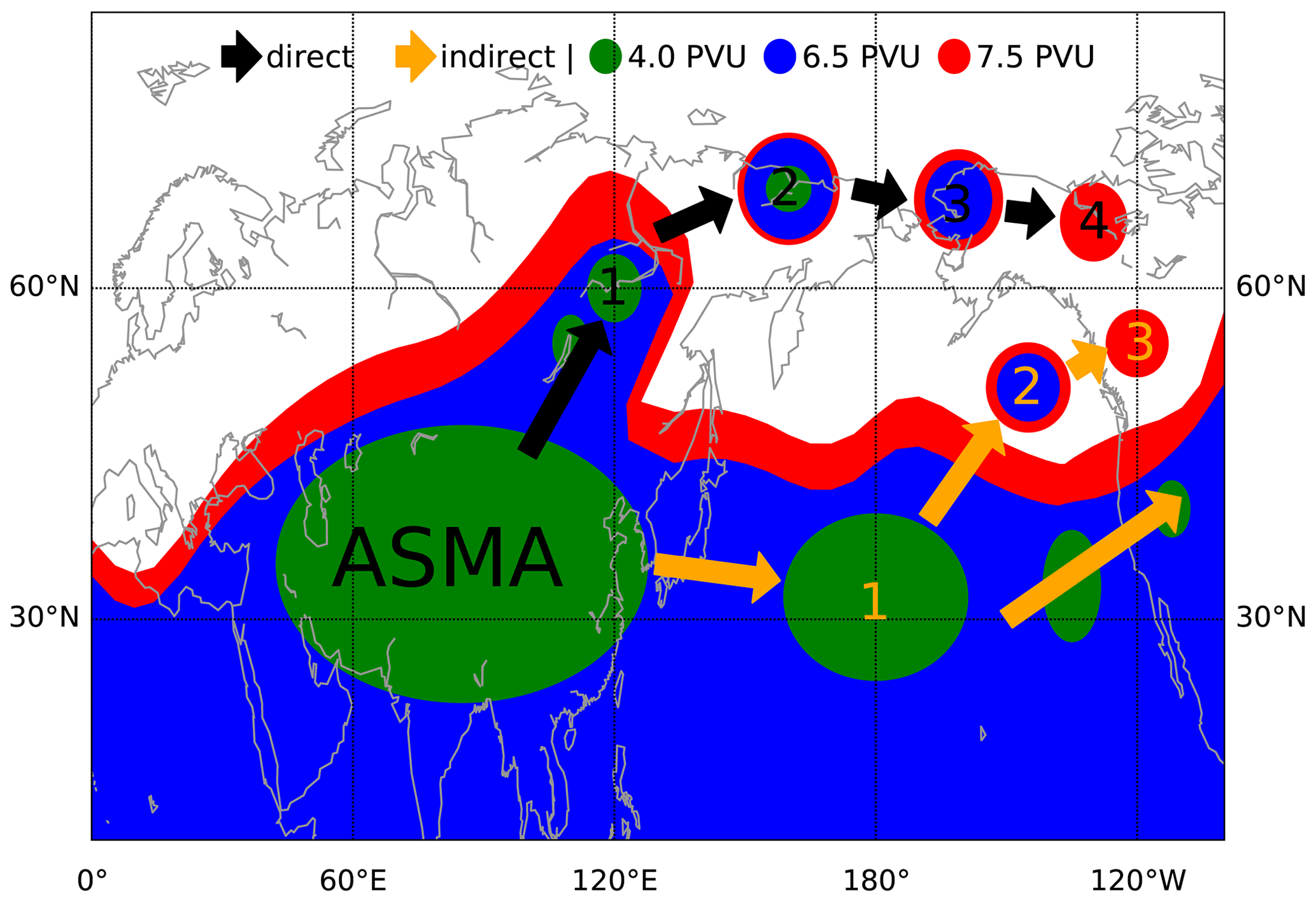
Figure 1 Schematic of the two idealized transport pathways from the ASMA into the stratosphere and the role of low PV cutoffs on 380 K for each of the pathways. Green areas mark cutoffs with PV ≤ 4.0 PVU, and blue marks areas with 4.0 PVU < PV < 6.5 PVU. Red shows areas with 6.5 PVU < PV < 7.5 PVU. The black arrows indicate the direct transport pathway, and the orange arrows indicate the indirect pathway. Numbers denote the temporal evolution of the cutoff evolution.

Figure 1 schematically illustrates the transport from the ASMA into the lower stratosphere and the role of low PV cutoffs for this transport along two characteristic pathways. The two pathways were chosen based on a manual analysis of shedding events and in accordance with former transport studies (e.g. Vogel et al., 2014; Kunz et al., 2015). The first pathway is characterized by the poleward shedding of PV cutoffs with fast transport into the stratosphere, including elongated streamers. The second pathway is characterized by a more zonal shedding from the ASMA into the tropical troposphere, with subsequent slower transport into the stratosphere. It remains an open question as to whether the underlying dynamical processes also differ. The first indirect transport pathway from the ASMA to the stratosphere starts with the shedding of a large-scale cutoff at the eastern flank of the ASMA (4 PVU cutoffs; see Fig. 1; the orange arrow from the ASMA to a cutoff is denoted with 1). After the shedding process, the cutoff moves eastward over the North Pacific and decays into smaller low PV cutoffs, all of which happens within the troposphere. During this process, air masses of the decaying eddy can be transported across the tropopause into the stratosphere (see the orange arrows from 1 to 3). The second direct transport pathway frequently starts at the northeastern side of the ASMA, with a strong bulging of the ASMA and the development of a low PV streamer (see the black arrow from the ASMA to a cutoff denoted with a black 1). The bulging of the ASMA is visible as a deformation of the 4.0 PVU contour, while the streamers are mostly visible as the deformation of the 6.5 PVU contour. As illustrated in the schematic, the streamers may contain 4.0 PVU cutoffs that are transported poleward. In the next phase, the streamer detaches as a 6.5 PVU cutoff (see the black arrow from 1 to 2). Subsequently, mixing processes further increase the PV value in these air masses such that they are only detectable as a 7.5 PVU cutoff and, finally, entirely mix with the background, thus causing troposphere-to-stratosphere transport (TST; see the black arrows from 2 to 4). Hence, the full life cycle of a low PV cutoff involves the sequence of air masses enclosed by 4.0, 6.5, and 7.5 PVU when being transported from the ASMA to high latitudes. In the following, we will investigate cutoffs with respect to these three PV thresholds to gain information about the cutoff life cycle from the detachment from the monsoon anticyclone to the mixing with the lower stratospheric background.

2.3 Cutoff detection and tracking

Figure 2 presents the generation of cutoffs during the first week of July 2017 as an example of the direct pathway. On 1 July, the PV contours encircling the ASMA start to bulge at the northeastern edge of the ASMA (around 45^∘ N, 100^∘ E; see Fig. 2a). During the next 3 d, a low PV streamer develops in that region that extends beyond 60^∘ N and covers parts of eastern Russia (Fig.2b–d). This streamer also contains small 4 PVU cutoffs (Fig. 2c, d). After 4 July, the streamer breaks up into several cutoffs. These cutoffs decay during the next 3 d (not shown). The magenta and yellow lines show the tracks of the low PV anomalies, as determined from the 4.0 PVU (yellow) and 6.5 PVU cutoffs (magenta). The tracks show the trace of the geometrical centre of a cutoff from its formation to the given sampling time. More precisely, we consider cascades which sometimes consist of multiple cutoffs at the same time, and we chose one arbitrary cutoff of the cascade for each time step. For strongly diverging cascades, spurious jumps can appear. To reduce the jumps in cascades with many, but relatively close, cutoffs, the geometrical centre of all cutoffs in the cascade is chosen.

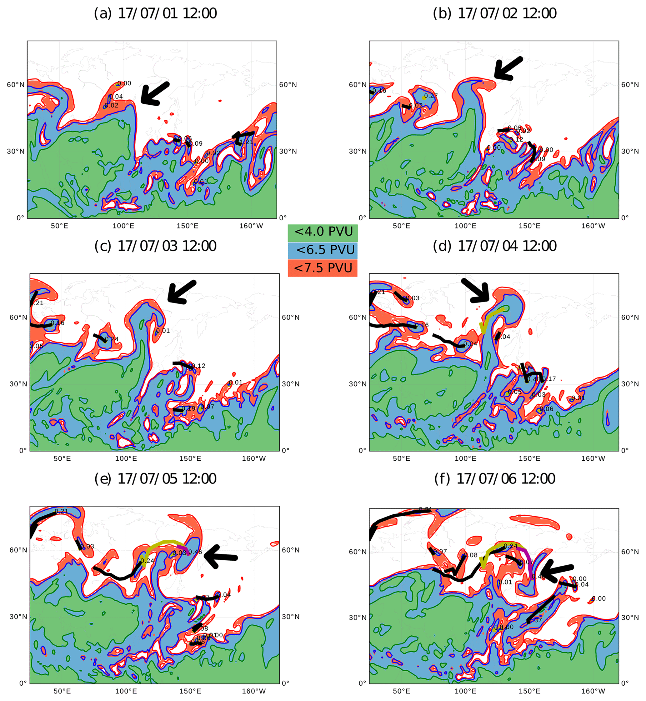
Figure 2 Example of the direct transport pathway from the ASMA into the lower stratosphere by cutoffs at 380 K in early July 2017 (see the dates at the top of panels). The black arrows point to the relevant streamers and cutoffs. The track of a small 4.0 PVU cutoff is shown in yellow, and the track of the subsequent 6.5 PVU cutoff is shown in magenta. The blue area marks the tropical troposphere (PV ≤ 6.5 PVU), and the green area marks the ASMA and the equatorial region (PVU ≤ 4.0 PVU). Red areas mark the mean tropical tropopause in JJA (June–August; PVU ≤ 7.5 PVU). Black lines show tracks of the 6.5 PVU cutoffs, and the text shows the maximum size of the cutoff in percent of the Northern Hemisphere.

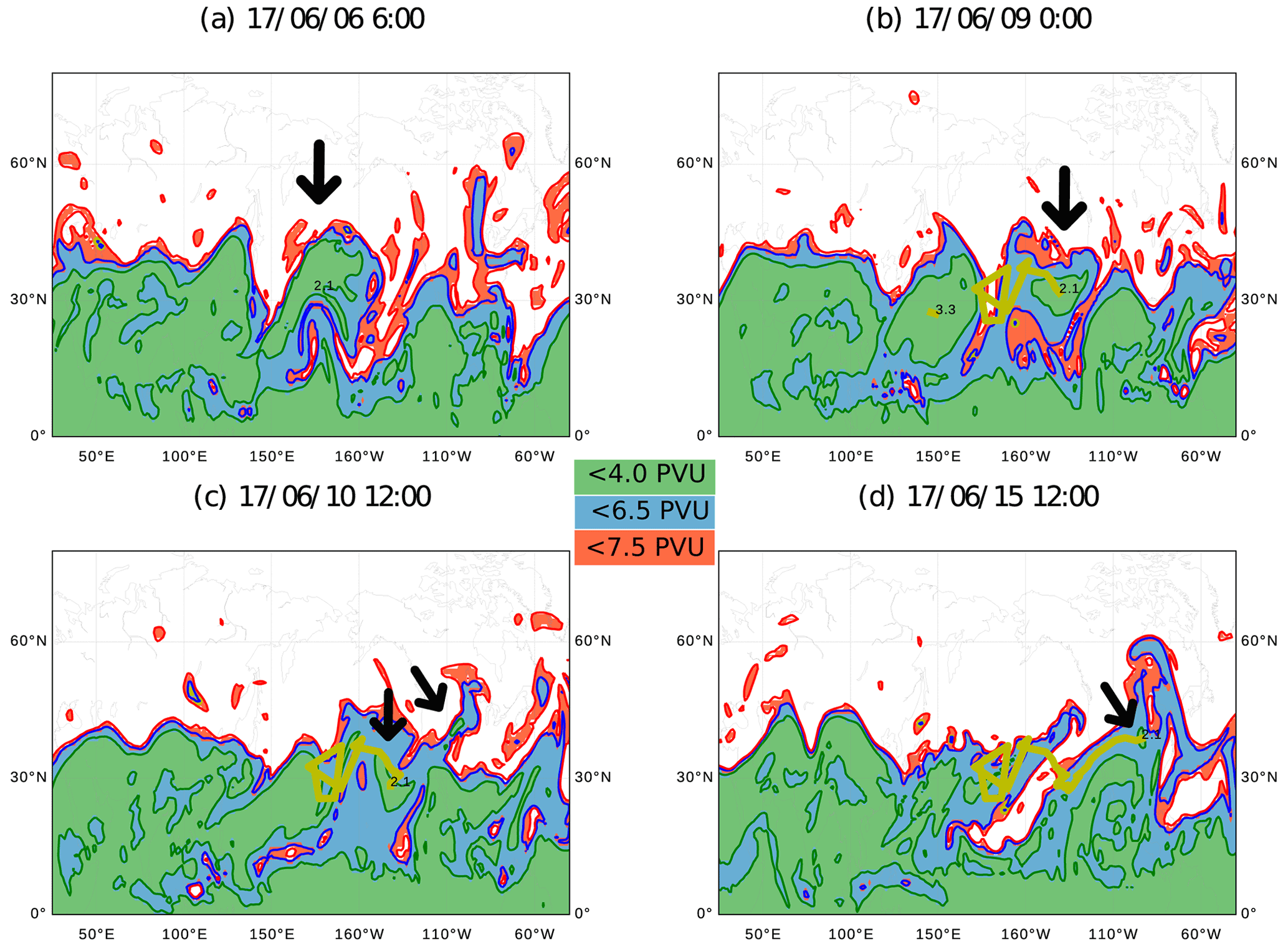
Figure 3 Example of the indirect transport pathway from the ASMA into the lower stratosphere by two eastward shed cutoffs from the ASMA at 380 K. Colours are as in Fig. 2. Yellow lines show tracks of the 4.0 PVU cutoffs. The largest cutoff (3.26 % of NH area) remains for only a very short time over the western Pacific. The smaller cutoff (2.12 % of the NH area) has a very long lifetime of about 1 week and travels to North America.

Examples for the indirect transport pathways, eastward eddy shedding, or ASMA splitting events can be found when considering the 4.0 PVU contours. These cutoffs are shed at the eastern edge of the ASMA and propagate eastward within the upper troposphere to Japan and the North Pacific (equatorward of the 6.5 PVU tropopause contour). Figure 3 shows the case of a cutoff that is shed from the ASMA (with respect to the 4 PVU contour) on 6 July 2017. After separating from the ASMA, the cutoff moves eastward over the North Pacific on the tropospheric side of the dynamical tropopause (7.5 PVU). Animations of the examples in this study can be found in the Supplement. The animations follow the structure of the Figs. 2, 3, and 10.

To extend the identification and the analysis of the cutoffs to climatological periods, we developed a dedicated algorithm. The general structure of the algorithm is illustrated in Fig. A1a. It consists of a part to determine the PV gradient tropopause, a part that detects the cutoffs, and a part that tracks the cutoffs. The cutoff identification and tracking in this paper is based on ERA-Interim reanalysis PV and wind data (see Sect. 2.1).

The tropopause detection algorithm is based on the work of Kunz et al. (2011). Therefore, the tropopause is defined as that PV contour where the gradient, with respect to the equivalent latitude of the product between zonal wind and PV, has its maximum. These tropopause PV contours are used to determine cutoffs exported from the tropical troposphere. The tropopause detection algorithm was used to identify the annual mean and the summer mean (JJA) tropopauses at the 380 K isentropic surface, which were found to be located along the 6.5 and 7.5 PVU contours, respectively.

The low PV cutoff detection algorithm was built upon the ideas of Wernli and Sprenger (2007). It essentially consists of a flood-fill algorithm that is applied step by step to all points in the PV field. Those coherent areas in the field with a PV value lower than a given threshold are marked with a unique number. The output of the algorithm is a field that marks grid points within cutoffs with the corresponding cutoff number, and the remaining areas of the stratosphere and tropical troposphere are marked with specific numbers. For the following analysis on the 380 K isentrope, the thresholds were set to 4.0, 6.5, and 7.5 PVU, representing the anticyclone edge, annual mean, and summertime mean tropopauses, respectively.

The tracking algorithm extends the methodology by Wernli and Sprenger (2007) and makes use of 2D​​​​​​​ Lagrangian trajectory calculations based on the Chemical Lagrangian Model of the Stratosphere (CLaMS; McKenna et al., 2002). A similar algorithm was recently developed by Portmann et al. (2021). The principal idea is to initialize air parcels within the detected cutoffs at time t₀, carry out a forward calculation of their trajectories over the time step Δt, and subsequently compare the new positions with the detected cutoffs at time $t_{\mathrm{1}}=t_{\mathrm{0}}+\mathrm{\Delta }t$. The time step Δt is here chosen as 6 h, which is equal to the analysis time step in ERA-Interim.

The tracking calculation from time t₀ to time t₁ needs the two cutoff index fields at these times, which are created by the detection algorithm. For each cutoff at time t₀, air parcels are initialized at the grid points within the cutoffs. These air parcels are calculated forward on the 380 K isentrope, using the CLaMS trajectory module (based on fourth-order Runge–Kutta scheme; see McKenna et al., 2002). For typical lifetimes of a few days for tropospheric cutoffs in the lower stratosphere, diabatic motions can be neglected, and a 2D isentropic trajectory calculation for the tracking is a valid approximation. After the advection time step Δt, the new positions are compared with the cutoff field at time t₁. In total, four different cases for a given cutoff are possible. First, the cutoff can persist so that some of the trajectories end within the same cutoff one time step later. Second, the cutoff may vanish during the time step or reconnect to the troposphere. In that case, the forward trajectories will not match a cutoff at time t₁. The third possibility is the splitting of the cutoff into two or more cutoffs. A fourth and last possibility is the merging of existing cutoffs into one new cutoff. In that case, the algorithm arbitrarily selects one of the previous cutoffs as the predecessor of the new cutoff. All these processes together can lead to complex connections between different cutoffs over multiple time steps, particularly if a large cutoff breaks down into many smaller ones. In the following, we will call a set of related cutoffs a cutoff cascade.

Finally, the chemical composition of the cutoffs is studied using chemical fields (H₂O, CO, and O₃) from simulations with the full-blown chemical transport model CLaMS. These simulations cover the period 2009–2018 and are driven with ERA-Interim reanalysis, such that the underlying meteorology is consistent with the detected PV cutoffs.

2.4 Filtering Asian monsoon cutoffs

This section presents the method to filter those cutoffs that transport air from the ASMA into the UTLS. This filtering method needs to take into account the existence of the two dominant pathways of low PV cutoffs from the ASMA, as presented earlier. ASMA-related cutoffs are distinguished from unrelated cutoffs with the help of the lifetimes, sizes, and locations of the cutoffs. The filter parameters were empirically chosen to fit results from a visual inspection of the relevant cutoffs during the period July–September 2017, as further detailed below.

Figure 2 shows an example for the direct transport pathway from the ASMA into the lowermost stratosphere (black arrows point to the cutoffs and streamers relevant for transport). During the event, several smaller 6.5 PVU cutoffs are found which propagate from western Russia or northern Europe into the ASMA region. Clearly, these cutoffs are not related to transport from the ASMA into the lowermost stratosphere. Such cutoffs unrelated to the ASMA often start westward of 45^∘ E and have maximum sizes below 0.3 % of the Northern Hemisphere area during their lifetime. Hence, we use a westward longitude boundary of 45^∘ E and a minimum size of 0.3 % of the Northern Hemisphere area to distinguish ASMA cutoffs from those unrelated to transport from the ASMA.

Figure 3 further presents an example for the indirect transport pathways, showing large eddies shedding eastward and remaining equatorward of the tropopause during the first days after detachment from the ASMA. The detailed analysis of cutoffs in June and July 2017 shows that the sizes of these eddies are between 0.5 % and 3.3 % of the Northern Hemisphere (NH) area. In contrast, the size of the observed ASMA varies between 5 % and 10 % of the NH area during this time. Therefore, a critical size of 3.5 % of the NH area was chosen to distinguish the ASMA itself from these cutoffs during June and July. In late August and September, the filtering by size does not work efficiently because of the decrease in the ASMA intensity and the frequent splitting of the 4.0 PVU contour. Eventually, the ASMA region inside the 4.0 PVU contour can be connected with the tropospheric reservoir. The ASMA then no longer appears as a 4.0 PVU cutoff, and no filtering is needed. To further constrain the filters, the initialization of the tracking calculation was restricted to the region between 25 and 180^∘ E and between 15 and 90^∘ N, where the ASMA is located, and the cutoffs of interest originate inside this region.

Table 1 Used filter criteria for the cutoffs in the ASMA region, based on the case study.

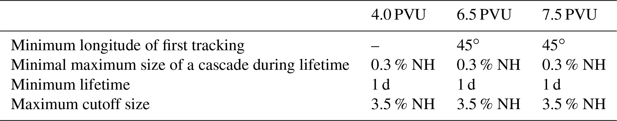
In summary, the following filter criteria are used to distinguish the cutoffs that are related to the ASMA from other cutoffs (see also Table 1). To filter cutoffs that propagate from far upstream into the ASMA region, we removed all cutoffs whose tracks start at longitudes westward of 45^∘ E. This filter was used for 6.5 and 7.5 PVU cutoffs. It is not used for 4.0 PVU cutoffs because they hardly originate so far upstream. To avoid small cutoffs that are not related to the ASMA, a minimum size of 0.3 % of the NH area during the cutoff lifetime and a minimum lifetime of 1 d has been chosen.

Although the presented case study already underpins the chosen filters, we additionally validated the filtering method with the help of additional trajectory calculations. For this purpose, backward trajectories have been initialized inside all detected ASMA cutoffs in summer (June–September – JJAS) 2017 to trace the cutoff air masses backwards in time and investigate whether they indeed originated in the ASMA. As a result, 93 % of the filtered 4.0 PVU cutoffs, 79 % of the 6.5 PVU cutoffs, and 96 % of the 7.5 PVU cutoffs were identified as being of ASMA origin and also in the backward trajectory calculation, further corroborating the filtering approach. Further details of the validation are discussed in the Appendix C.

3 Diagnosis of troposphere-to-stratosphere transport associated with low PV cutoffs

3.1 Seasonality in the extratropical UTLS

To interpret transport by low PV cutoffs from the ASMA within a global context, we first consider the global frequency distributions of all low PV cutoffs (PV < 6.5 PVU) on 380 K in all seasons (Fig. 4) and also include those low PV cutoffs that are not related to the ASMA. Following Wernli and Sprenger (2007), the presented seasonal mean frequency quantifies the fraction of times (relative to all time steps in a season) when a grid point is covered by a cutoff. For example, a value of 1 % indicates that, during 1 % of the time, this point is covered by a cutoff.

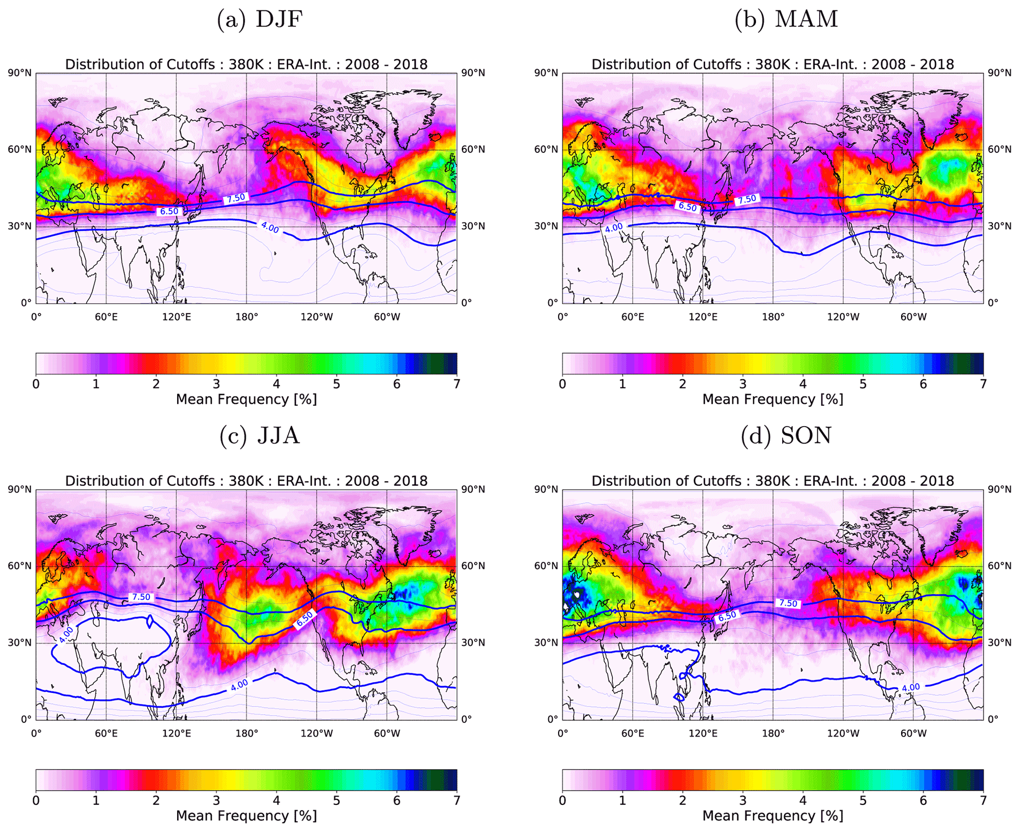
Figure 4 Global climatological frequency distribution of 6.5 PVU cutoffs in the four seasons. A 1 % mean frequency means that, in 1 % of the time steps during a season, a cutoffs covers the point.

From autumn to spring (September–November, SON, December–February, DJF, and March–May, MAM), similar patterns can be observed which are characterized by a band of high cutoff activity that extents from the west coast of North America over the Atlantic and Europe to central Asia. Transport activity, as measured here by the cutoff frequency, peaks in the Atlantic–European region and is strongest during autumn (SON). Furthermore, during autumn, winter, and spring, only weak transport activity related to low PV cutoffs can be found over the Pacific. These patterns agree well with results from past studies by Kunz et al. (2015).

During boreal summer, the cutoff frequency distribution changes significantly. A strong peak in the low PV cutoff frequency emerges over the central North Pacific at about 30–50^∘ N. The location of that peak downstream of the ASMA region and the weak gradients in the PV distribution between the peak and Southeast Asia suggest that these cutoffs are likely related to transport from the Asian monsoon. This Pacific region with high cutoff frequency extents northward to Siberia and Alaska, indicating long-range transport from low to high latitudes. Hence, the Asian monsoon appears to strongly affect the distribution of low PV cutoffs in the NH and related transport, with air masses exported from the ASMA preferentially affecting the stratosphere over the North Pacific.

3.2 Asian-monsoon-related transport

In the following, we focus on low PV cutoffs on the 380 K isentrope that are directly related to the ASMA. Section 2 explained how these cutoffs were identified and that it is meaningful to identify low PV cutoffs related to the ASMA with PV threshold values of 4.0, 6.5, and 7.5 PVU, respectively.

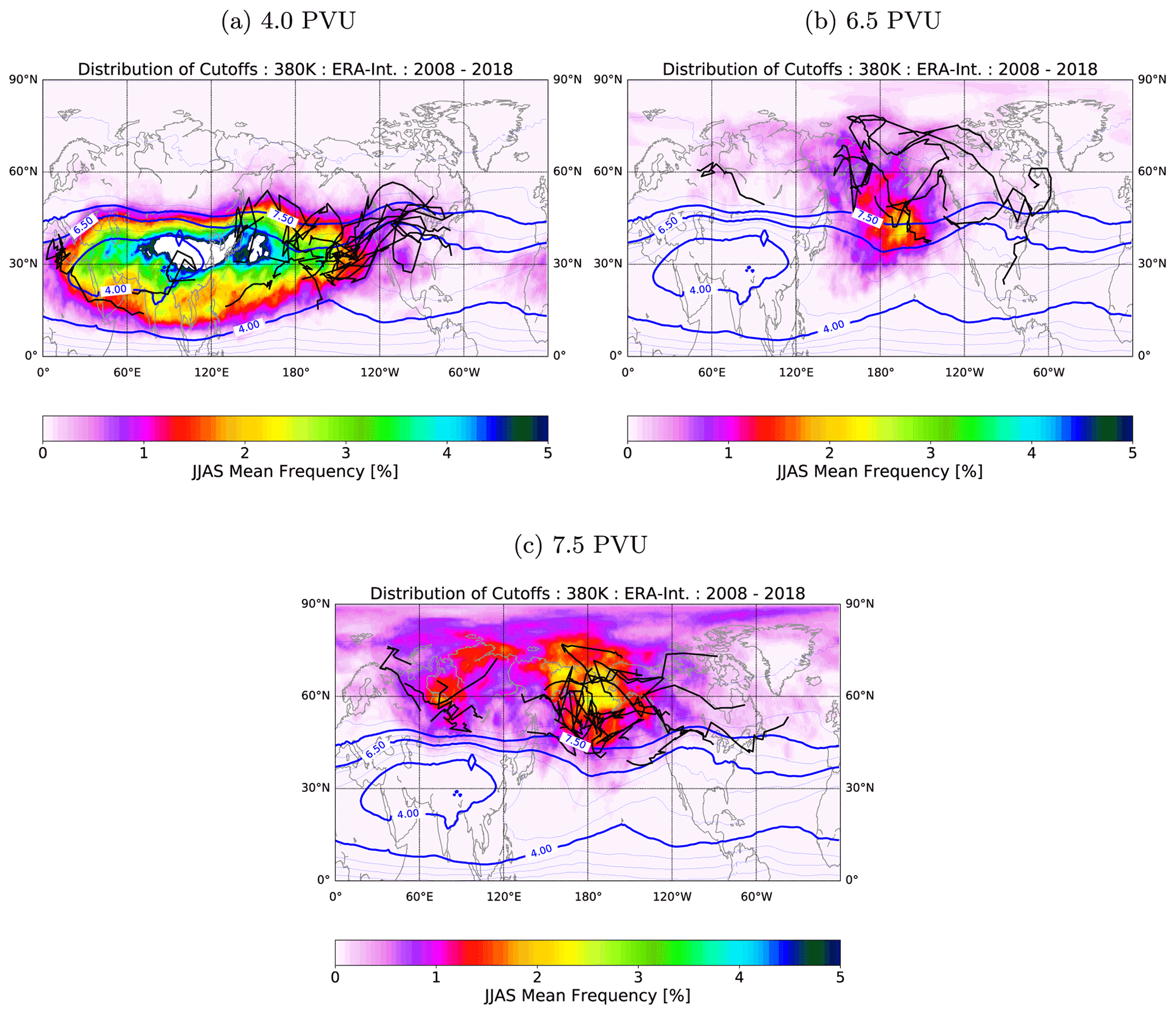
Figure 5 Climatological frequency of ASMA-related cutoffs during JJAS, for (a) 4.0 PVU cutoffs, (b) 6.5 PVU cutoffs, and (c) 7.5 PVU cutoffs. The blue lines indicate particular PV contours. A subset of the identified tracks with a lifetime of at least 4 d is plotted with black lines. Here, 1 % means that a point is covered with a cutoff in 1 % of the time steps in JJAS. Frequencies higher than 5 % are coloured white.

Figure 5a shows the JJAS distribution of ASMA cutoffs on 380 K with respect to the 4.0 PVU contour. The frequency distribution indicates the transport of air masses exported from the anticyclone. These ASMA–cutoffs mainly leave the anticyclone above eastern China and then move downstream of the ASMA along about 35^∘ N latitude, reaching Japan and the Pacific region. Some of the cutoffs propagate even to North America. The peak in monsoon air over Japan in this season has recently been found in an independent analysis and has been described as a particular mode of the anticyclone (Honomichl and Pan, 2020). The zonal and eastward transport also resembles the eastward eddy shedding found in theoretical studies (e.g. Rupp and Haynes, 2021). The westward transport from the ASMA is comparably low, but weak cutoff activity extends zonally, even to Morocco, possibly indicating westward shedding (e.g. Hsu and Plumb, 2000; Popovic and Plumb, 2001). However, since the climatological ASMA and westward shed eddies can overlap, our method misses some cutoffs in this region. Overall, the ASMA cutoffs mainly distribute between the 6.5 PVU tropopause on 380 K and the 4.0 PVU contour near the Equator, showing that the related transport is mainly zonal and restricted to the troposphere.

The frequency distribution of cutoffs with PV < 6.5 PVU indicates the transport of air from the ASMA across the subtropics into the middle latitudes (Fig. 5b). As already indicated by the seasonal plots in Fig. 4, the cutoffs are most frequent above Siberia and the North Pacific. The location of the peak intensity just downstream of the maximum frequency of the ASMA cutoffs indicates the relation between the two types of detected cutoffs, with 6.5 PVU cutoffs likely representing a later stage and the 4.0 PVU cutoffs representing an earlier stage of the cutoff life cycle.

Finally, the cutoff distribution with PV < 7.5 PVU indicates the transport of ASMA air further into NH middle and high latitudes (Fig. 5c). Peak intensity occurs above the North Pacific just north of the frequency peak of the 6.5 PVU cutoffs. This indicates that the 7.5 PVU cutoffs represent again a later transport stage when the ASMA air moves to even higher latitudes with continuously increasing PV, as compared to the 6.5 PVU cutoffs. In addition to the peak over the North Pacific, enhanced cutoff frequency also occurs above Siberia, and a few 7.5 PVU cutoffs even reach the pole. The 7.5 PVU cutoff frequency is higher than the frequency of the 6.5 PVU cutoffs due to the larger extent of the former cutoffs.

Furthermore, the frequency distribution of ASMA cutoffs shows considerable sub-seasonal variability. ASMA cutoff activity starts in June and becomes strongest during July and August (see Appendix Fig. B1). Also, September still shows frequent ASMA cutoffs, with the highest occurrence above Alaska.

For the transport to Siberia (around 80^∘ E) the cutoff stages at 4.0 and 6.5 PVU appear not to be relevant, but only the 7.5 PVU stage is considered relevant (see Fig. 5). On the other hand, our validation with 30 d backward trajectories establishes a clear relation to the ASMA. Also, the jet is very strong at 60^∘ E but still has sporadic cutoffs, presumably due to the Rossby wave breaking (RWB) that could be created there. One possible explanation for high 7.5 PVU cutoff frequencies over Siberia could be that air encircles the ASMA in a clockwise manner in its outer areas, possibly ranging far west, and subsequently merges with the jet stream on its way back. When there is RWB between 30 and 60^∘ E (see Fig. 4; JJA), the air mass could be transported into the stratosphere.

3.3 Characterization of cutoffs in time and space

Cutoff characteristics, like their lifetime, size, and the maximum latitude reached, are closely related to the transport and atmospheric composition. Figure 6 presents the probability density functions (PDFs) and cumulative density functions (CDFs) of these properties for the cutoffs related to the ASMA, with the individual distributions shown for the three cutoff stages (4.0, 6.5, and 7.5 PVU), respectively.

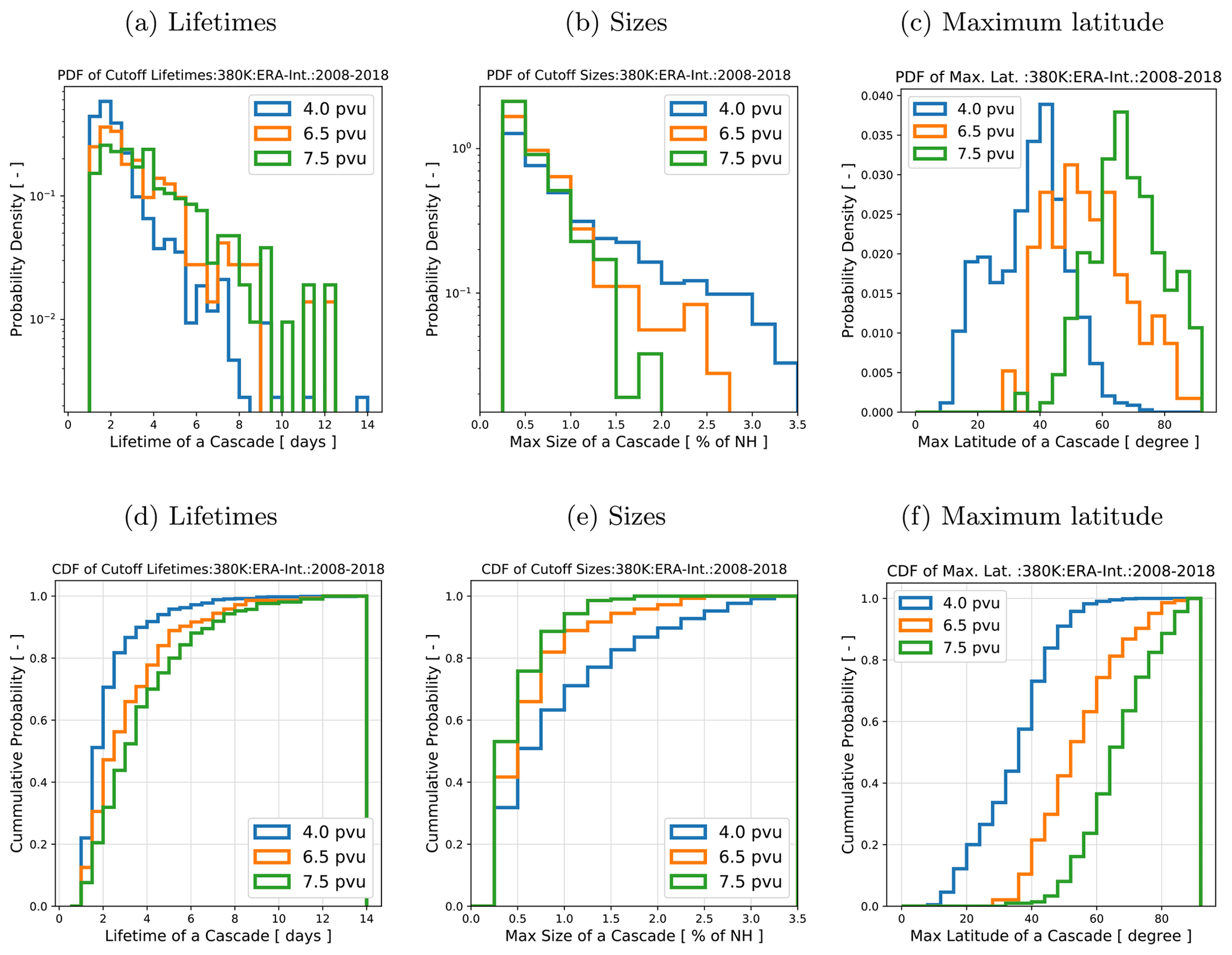
Figure 6 PDFs (a–c) and CDFs (d–f) for the lifetime, size, and maximum latitude of ASMA-related cutoffs at 380 K between 2008 and 2018. The frequencies are determined from the number of cutoffs.

The probability distribution of lifetimes is shown in Fig. 6a and d (note the logarithmic scale). The distributions are similar for the three stages and characterized by a high frequency of short lifetimes and a low frequency of long lifetimes. Between 90 % and 98 % of the cutoffs exist for less than 1 week. Most of the cutoffs have a very short lifetime between 1–3 d, and the distribution shows a long tail with rare events with lifetimes up to 2 weeks. The tail of the distribution is somewhat stronger for the cutoffs at later stages (6.5 and 7.5 PVU), indicating more long-lived events for these categories.

A probability distribution of the maximum sizes in a cutoff cascade is shown in Fig. 6b and e (note the logarithmic scale). More than 50 % of the cutoffs have a size between 0.3 % and 0.75 % of the NH area. The distributions have a strong tail up to sizes of about 2.0 % (7.5 PVU), 2.7 % (6.5 PVU), and 3.5 % (4.0 PVU) of the NH area, and they all peak at the smallest bin size considered. Larger cutoffs appear to contribute more significantly to the ASMA cutoffs directly after detachment from the anticyclone (4.0 PVU cutoffs), compared to the cutoffs detected at later stages (6.5 and 7.5 PVU). Hence, the ASMA is a source of large-scale cutoffs, likely originating from shedding processes or even splitting of the ASMA. Splitting events happen mainly in August and September when the ASMA weakens, and this presumably explains most of the largest cutoffs.

A view of the distributions of the maximum latitude a cutoff reaches (Fig. 6c, f) shows that the ASMA cutoffs are mainly restricted to latitudes below 50^∘ N, stressing the fact that they contribute mainly to zonal transport in the troposphere. On the other hand, the frequency of maximum latitudes for cutoffs at a later stage (tropospheric 6.5 PVU cutoffs) peaks near 50^∘ N. This again emphasizes the importance of considering the later stage of cutoff events for long-range meridional transport.

As the low PV cutoffs decay, i.e. their PV increases to typical stratospheric background values, they become smaller and mix with stratospheric air. Figure 7 shows the evolution of the size of the tropospheric 6.5 PVU cutoffs with a lifetime longer than 5 d (note the logarithmic scale). In contrast to the size of the largest cutoff within a cascade (as in Fig. 6b, e), here the individual sizes of all cutoffs within a cascade are shown as a function of a lifetime. Hence, intermediate sizes below the filter criteria of 0.3 % are possible, as long as the size of one cutoff in the full cascade at some point exceeds the threshold. On average, the cutoff size decreases gradually over time, showing an approximately exponential decay with a half-lifetime of around 3 d. For some cutoffs, their size stays nearly constant for a while and then suddenly decreases – or even increases. This behaviour is in accordance with the variability in the cutoff pathways and with the physical processes that affect PV and, therefore, the size of the cutoff along these pathways. A sudden decay, for example, can appear if a cutoff crosses the tropopause, while a strong interim increase in size can result from the collision and merging of two cutoffs.

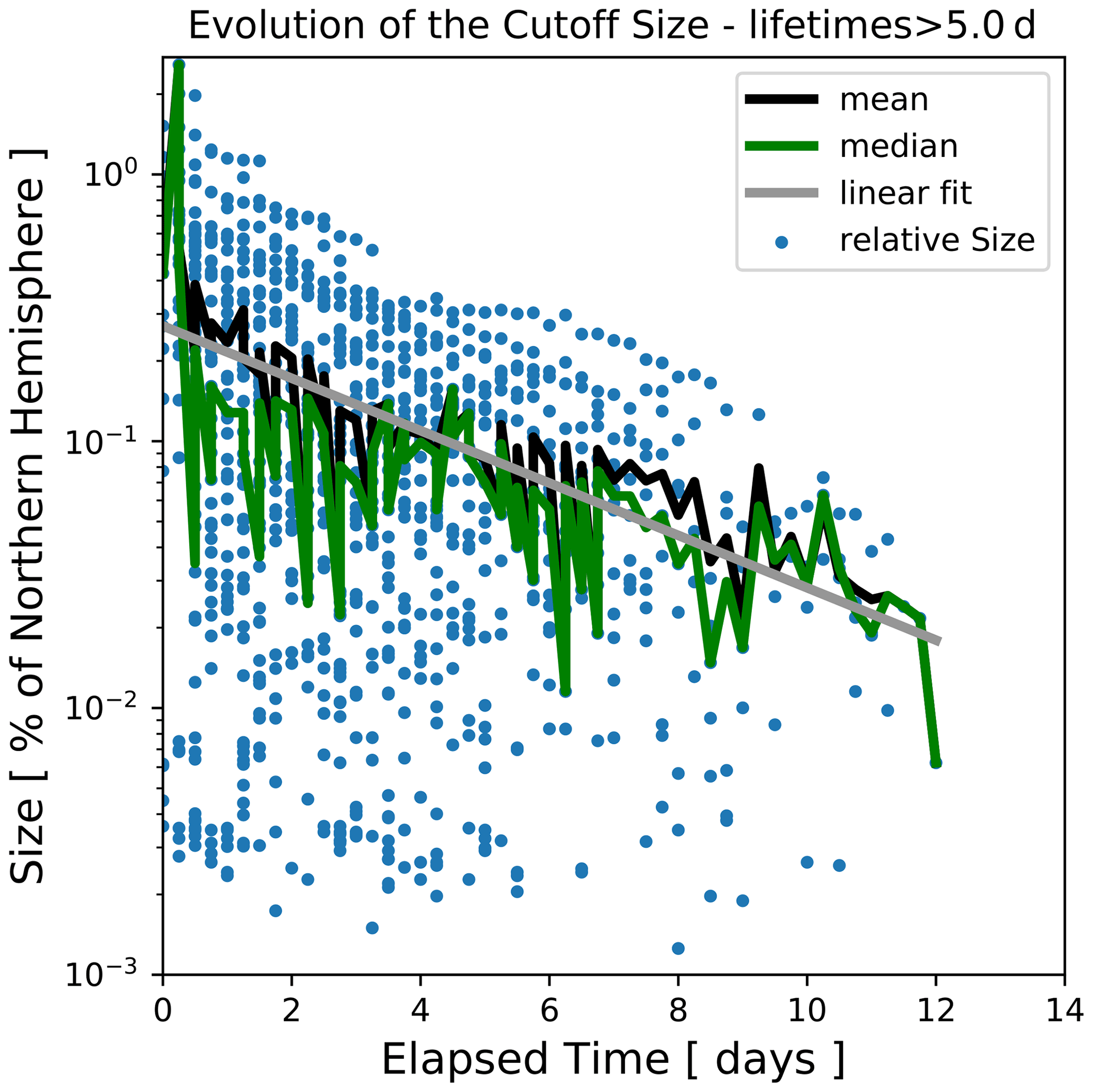
Figure 7 Decay of cascades of 6.5 PVU cutoffs, for cascades that live longer than 5 d. The blue dots show the relative sizes in percent of the NH of each cutoff within the cascade. Note that a cutoff of a cascade can have sizes below 0.3 % of the NH, while the largest cutoff of the cascade can still exceed the threshold of 0.3 % at some time.

4 Chemical composition

The low PV cutoffs separated from the Asian monsoon anticyclone are characterized by anomalous tracer concentrations, indicating young tropospheric and highly polluted air masses. Hence, such cutoffs provide a pathway for polluted tropospheric air into the lowermost stratosphere. To further investigate the chemical evolution within the cutoff air, we analyse the mixing ratios for CO, H₂O, and O₃ in the cutoffs and compare them with the typical values for the entire troposphere and stratosphere, respectively.

Figure 8 Chemical composition of the ASMA and tropospheric cutoffs at 380 K. Shown are histograms and PDFs of the mixing ratio of (a) CO, (b) H₂O, and (c) O₃, which are all simulated with CLaMS. The histograms are plotted with dotted lines. The related axis is always on the left. The histograms show the frequency of the mixing ratios within the different spheres of the atmosphere. Additionally, PDFs are shown with solid lines. The related axis is on the right. The probability density shows the frequency of the mixing rations during the different stages of the cutoffs.

Figure 8 shows the mixing ratio distributions for CO, H₂O, and O₃. First, the calculated dynamical tropopause appears to be in good agreement with the chemical separation between the stratosphere and the troposphere, as mixing ratios for air masses characterized by PV values above and below the tropopause value clearly differ. As indicated in Fig. 8, the mixing ratio distributions for CO and O₃ for the entire atmosphere show a clear bimodal structure. The peak with high CO and low O₃ mixing ratios is related to the upper troposphere, while the low CO and high O₃ peak is related to the lower stratosphere. For H₂O, the separation between upper tropospheric and lower stratospheric mixing ratios in the global distribution appears less clear due to a large overlap between the two peaks. This overlap is likely related to the fact that, for H₂O, the chemical separation is better described by the cold point tropopause than the dynamical tropopause used here.

The mixing ratios of air masses just exported from the ASMA are represented by the distributions for the 4.0 PVU cutoffs. These distributions show evidence that the ASMA contains the highest CO, the lowest ozone, and the highest water vapour mixing ratios, corroborating the role of the ASMA as a source for tropospheric, highly polluted air.

The chemical evolution in the cutoff air masses becomes clear from a comparison of the ASMA cutoffs at different stages during their life cycle (4.0, 6.5, and 7.5 PVU cutoffs). At the later stage (6.5 and 7.5 PVU), the cutoffs show relatively broad mixing ratio distributions that maximize between the tropospheric and the stratospheric peaks. These intermediate chemical characteristics of the cutoffs between troposphere and stratosphere are consistent with the evolution of the cutoffs during transport from the ASMA into the lower stratosphere and related mixing with the surroundings. At the latest stage during the cutoff life cycle (7.5 PVU), just before mixing with the lower stratospheric background, the cutoffs are characterized by mixing ratios with the strongest stratospheric character. For these cutoffs, the CO mixing ratios are lower and O₃ mixing ratios are higher, compared to the 6.5 PVU cutoffs, and already close to the background values in the lower stratosphere.

In the following, we further analyse the chemical evolution in the cutoffs over the cutoff life cycle.

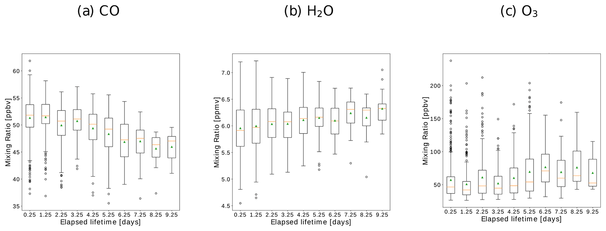
Figure 9 Chemical evolution of the chemical species of (a) CO, (b) H₂O, and (c) O₃ within the exemplary PV cutoff of Fig. 3. The box-and-whisker plots show the upper and lower quantile, the median (orange line), and the average (green pyramid) of the mixing ratios for each time step during the lifetime of the PV cutoff cascade. The black dots show the outliers.

To illustrate the early stage of the cutoff life cycle, Fig. 3 shows a cutoff that is shed from the ASMA (with respect to the 4.0 PVU contour) on 6 July 2017. After separating from the ASMA, the cutoff moves eastward over the North Pacific on the tropospheric side of the dynamical tropopause (7.5 PVU). The chemical composition in the cutoff changes continuously during the eastward propagation, without large steps (Fig. 9). CO shows a strong decrease in mixing ratio, caused by mixing with stratospheric background air and chemical loss, while O₃ mixing ratios are increasing during eastward propagation. The water mixing ratio shows only a small positive trend.

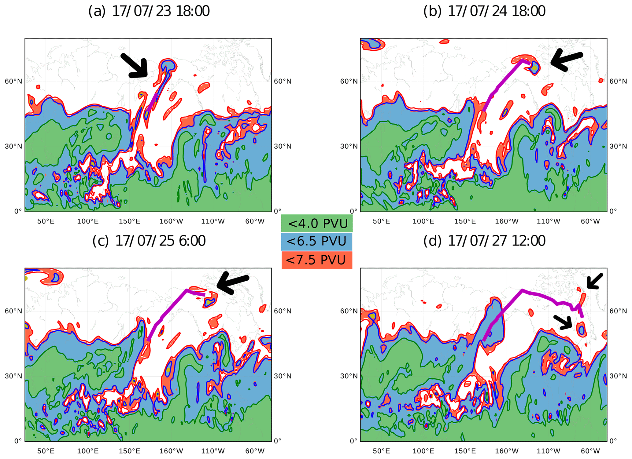
Figure 10 Example of an eastward shed 7.5 PVU cutoff from the ASMA at 380 K. Colours are as in Fig. 2. The violet line shows the track of the moving 7.5 PVU cutoff.

Figure 11 Chemical evolution of the chemical species of (a) CO, (b) H₂O, and (c) O₃ along the exemplary PV cutoff shown in Fig. 10. Box-and-whisker plots are as in Fig. 9.

The final stage of the cutoff life cycle before mixing with the stratospheric background is illustrated by showing an example of a 7.5 PVU cutoff in Fig. 10. The small 7.5 PVU cutoff forms around 23 July 2017 above the North Pacific and moves further northeastward until 27 July. This cutoff moves fast over a long distance and transports tropospheric air deep into the high-latitude stratosphere. Also, the cutoff contains well-defined 6.5 PVU cutoffs (closed contours) for some time. After passing over Alaska and parts of Canada, the cutoff finally mixes with stratospheric air and disappears. As shown in Fig. 11, the CO and H₂O mixing ratios slightly decrease over about the first 5 d, while the O₃ mixing ratios weakly increase. After the fifth day, stronger mixing ratio changes occur, which is likely related to interaction with other cutoffs and mixing over the eastern part of North America.

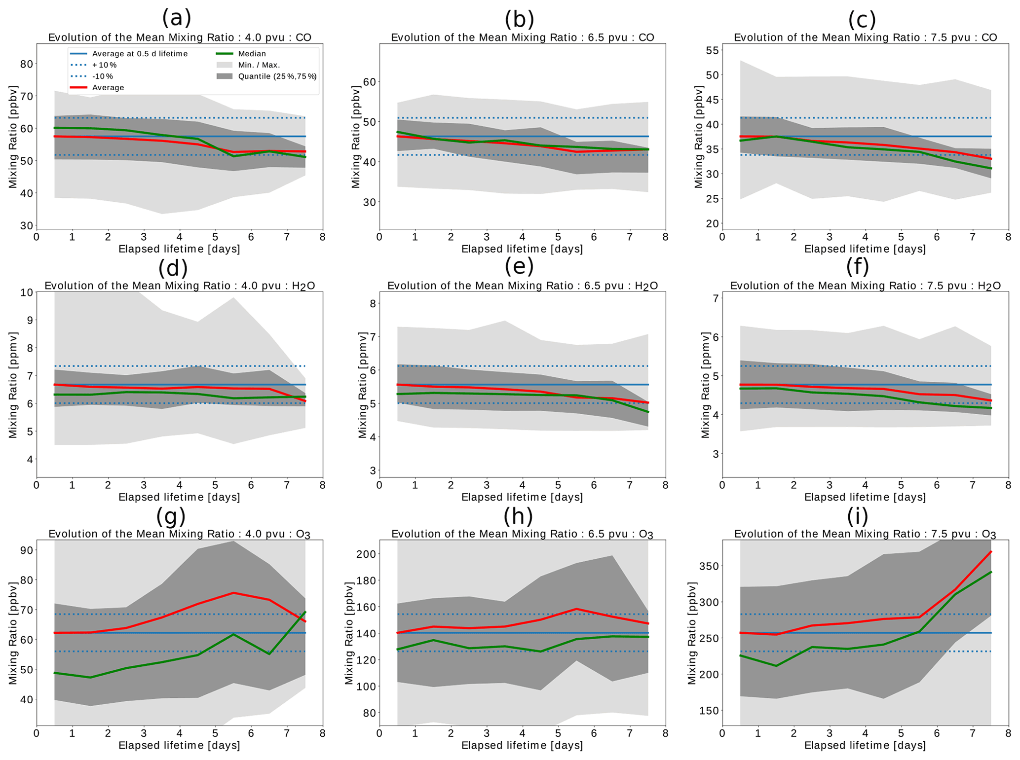
Figure 12 Mean evolution of CO (a–c), H₂O (d–f), and O₃ (g–i) mixing ratios with respect to the 4.0 PVU cutoffs (a, d, g), 6.5 PVU cutoffs (b, e, h), and 7.5 PVU cutoffs (c, f, i). The mean evolution has been calculated by averaging over all cutoffs with a minimum lifetime of 3 d from 2008 to 2018. The red line shows the mean value and the green line the median for every time step. Dark grey areas show the range between the upper and lower quantile, and the light grey areas show the minimum–maximum range. The blue solid lines indicate the average at day 0.5 and the dotted blue lines the ±10 % range from this average.

A statistical analysis of the chemical evolution in all cutoffs during 2008 to 2018 is presented in Fig. 12. The figure shows the mean evolution of CO, H₂O, and O₃ mixing ratios in the 4.0, 6.5 and 7.5 PVU cutoffs over 1 week (cutoffs with lifetimes of at least 3 d are included). For CO, the mean mixing ratio in ASMA cutoffs is about 60 ppbv (parts per billion by volume). Over 1 week, the mean CO mixing ratio decreases by about 10 % (Fig. 12a–c). A similar percentage change occurs for the 6.5 and 7.5 PVU cutoffs over the same period. This similar mean decrease rate for the different cutoffs is related to gradual mixing of the cutoffs with stratospheric air masses and chemical decay (the chemical lifetime of CO in the UTLS is about 2–3 months).

For H₂O, the mean mixing ratio in the 4.0 PVU cutoffs stays largely constant and is related to the fact that H₂O is controlled by processes mainly at the tropopause. Indeed, for the 6.5 and 7.5 PVU cutoffs, which represent cross-tropopause transport, the H₂O mean mixing ratio also changes. However, this mean H₂O change is very weak (about 10 % over 1 week) compared to H₂O changes at the tropical tropopause, related to the fact that the extratropical stratospheric H₂O distribution is only very weakly affected by subtropical tropopause temperatures (Hoor et al., 2010), such that mixing with background air controls the composition of the cutoffs. The stratospheric tracer O₃ shows increasing mixing ratios in the cutoff air masses over the cutoff life cycle (Fig. 12g–i). The strongest O₃ increase occurs in the 7.5 PVU cutoffs, when mixing with the high-ozone stratospheric background air occurs. This mixing changes the mean mixing ratio from about 250 to 375 ppbv, which is about 50 %.

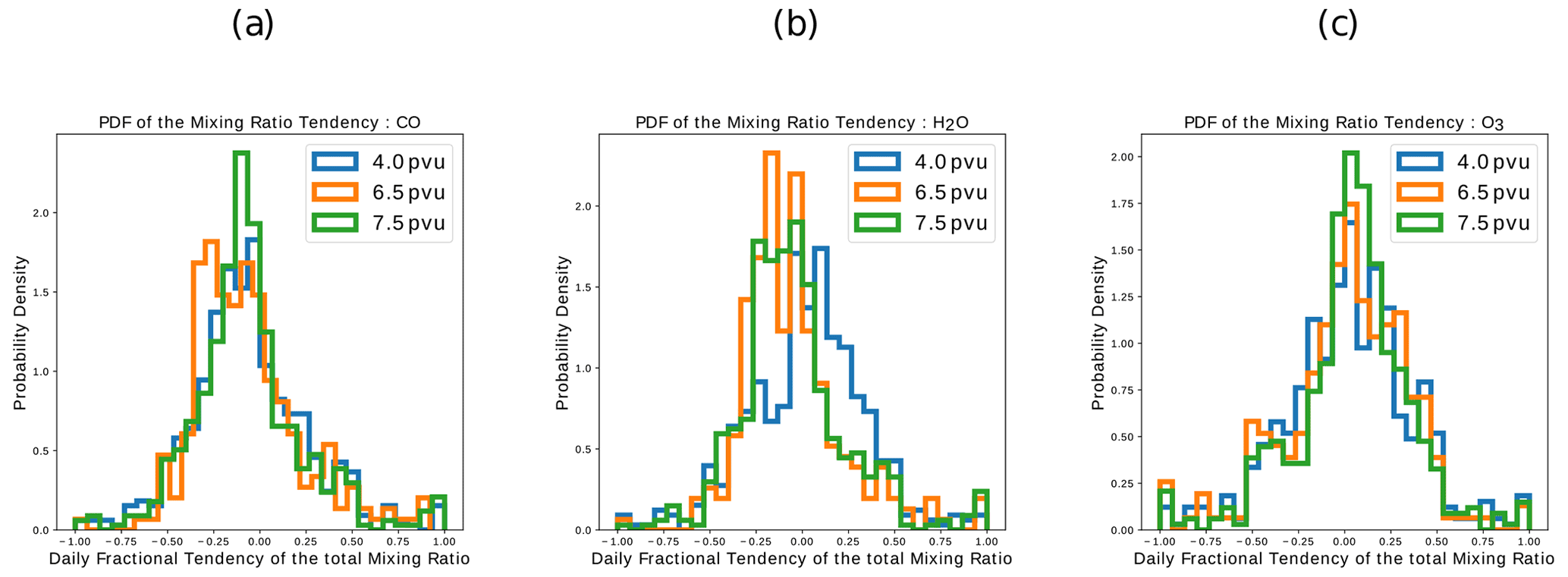
Figure 13 PDFs of the daily tendencies of the mixing ratios averaged within ASMA-related PV cutoffs. The tendencies – changes in mixing ratio per day – were normalized to the minimum–maximum mixing ratio range of each cascade. Only cascades with lifetimes of 3 d or longer are included.

The mixing of the cutoff with the stratospheric background and the related change in chemical composition can occur either gradually over the cutoff life cycle, or in strong individual events (e.g. sudden break-up of the cutoff). To further investigate the respective roles of these two possibilities, Fig. 13 shows the PDFs of the mixing ratio changes (daily change relative to the net change over the entire lifetime) for CO, H₂O, and O₃ and for the 4.0, 6.5, and 7.5 PVU cutoffs. For all species, the distributions peak close to zero. For CO and H₂O, the peak occurs at weakly negative tendencies, consistent with the general decrease in mixing ratios over the life cycle. For O₃, on the other hand, the peak occurs at slightly positive mixing ratios, consistent with a general mixing ratio increase caused by mixing with stratospheric background air. The existence of these strong peaks at very small changes shows the dominant role of slow and gradual processing in the cutoffs, which is related to continuous mixing with stratospheric background air, and the additional effects of chemistry (decay for CO and production for O₃). However, strong singular mixing events are not entirely negligible for the chemical composition change in the cutoffs, as the apparent tails of the PDFs show. The non-zero PDF values at ±1 show a non-vanishing probability for the entire mixing ratio change in a cutoff to occur within 1 d, and this can be related to a sudden cutoff decay or the merging of different cutoffs.

5 Discussion and conclusions

In this study, we investigated low PV cutoffs that transport air masses from the ASMA into the extratropical lower stratosphere. A new cutoff detection and tracking method was developed to identify the cutoffs in the Northern Hemisphere PV field and to calculate their tracks. Spatial and temporal filters have been applied to relate the cutoffs to the ASMA.

In total, two dominant pathways for transport from the ASMA to the stratosphere have been identified, which we termed the direct and indirect pathway, respectively. In both cases, the transport starts with cutoffs that shed as 4.0 PVU contours from the ASMA. These cutoffs show distinct high CO, low O₃, and high H₂O anomalies in the upper troposphere. In case of the indirect pathway and in the early stage of the cutoff life cycle, the cutoffs are mainly located near the ASMA over Japan. These cutoffs are relatively large and propagate eastward. During eastward propagation, the cutoffs decay and break up into smaller cutoffs. The remaining smaller cutoffs are transported further towards North America and even further away. Subsequently, the cutoffs decrease in size, and their chemical characteristics change gradually towards lower CO and higher O₃ mixing ratios, likely related to continuous mixing with stratospheric background air that is not of ASMA origin.

In the case of the direct pathway and in the early stage of the life cycle, the cutoffs emerge from streamers at the northeastern flank of the ASMA. These air masses can be identified as 4.0 PVU cutoffs within 6.5 PVU streamers and are of small to medium size. A few days later, the 6.5 PVU streamers break up, and the PV of the cutoffs increases. Consequently, the remaining PV anomalies can only be identified with the criterion PV ≤ 6.5 PVU (not 4.0 PVU anymore). In this stage, the cutoffs are located typically over eastern Russia or the North Pacific and still contain polluted air of ASMA origin. Later, the PV of the 6.5 PVU cutoffs again increases further, such that the cutoffs at an even later stage can only be identified as anomalies with PV ≤ 7.5 PVU, i.e. they form tropospheric cutoffs embedded in the lower stratosphere (recall that 7.5 PVU is the dynamical tropopause on 380 K). The transition from 6.5 PVU cutoffs to 7.5 PVU cutoffs takes place during the eastward transport above the North Pacific. At the same time, the chemical composition of the cutoffs approaches stratospheric background values with decreasing water vapour and CO and increasing O₃.

Overall, the highest frequency of horizontal transport from the anticyclone across the tropopause occurs over the North Pacific from July to August, such that this region and season appears most promising for measuring such air masses.

All types of cutoffs show skewed PDFs for their lifetimes and sizes, revealing the existence of a multitude of small-scale, short-lived cutoffs and only a few larger-scale and long-lived cutoffs. The temporal characterization of the cutoffs reveals an average lifetime of the cutoffs of around 3 d. Moreover, more than 90 % of the cutoffs have a lifetime shorter than 1 week. Larger cutoffs are more frequent during the early stage than during later stages of the overall transport process. The cutoff size decreases approximately exponentially, with a half-life of around 3 d. However, there is large case-by-case variability.

We found that cutoffs contribute to the transport from the ASMA to the stratosphere and, hence, to the troposphere-to-stratosphere mass flux. This leads to a few new questions with regard to their role for TST, namely (i) how large is the irreversible mass flux in relation to other irreversible TST processes? (ii) What types of cutoffs contribute mostly to the mass flux (i.e. a few large or many small cutoffs)? (iii) How do the transport processes change (e.g. in terms of lifetimes and frequency distributions of the cutoffs) with changing background conditions, such as a changing jet stream or a changing thermal forcing of the ASMA?

Moreover, the correct representation of the life cycle of cutoffs from the ASMA and their coupling to chemistry is important for climate models to correctly represent the transport of anthropogenic pollution into the lower stratosphere. Therefore, the development of detailed diagnostics for evaluating the sources, transport, and chemical composition of the cutoffs, as presented in this study, is crucial.

Appendix A: Cutoff tracking schematic

The tracking algorithm relates cutoffs at the two consecutive time steps of t₀ and t₁. Therefore, air parcels are initialized at t₀ within all found cutoffs. Subsequently, the trajectories of the air parcels are calculated forward for 6 h. The new positions of the parcels are compared with the position of the cutoffs at time step t₁. Where there is overlap between a cutoff and the forward-calculated air parcels, the cutoffs are assumed to be related. For the case of merging, forward-calculated parcels of multiple cutoffs end up in one cutoff. In this situation, an arbitrary cutoff is chosen to be the parent of the merged one. Other cutoffs are ignored. Figure A1a gives an overview of the structure of the programme, and Fig. A1b shows how the programme handles different kinds of cascades.

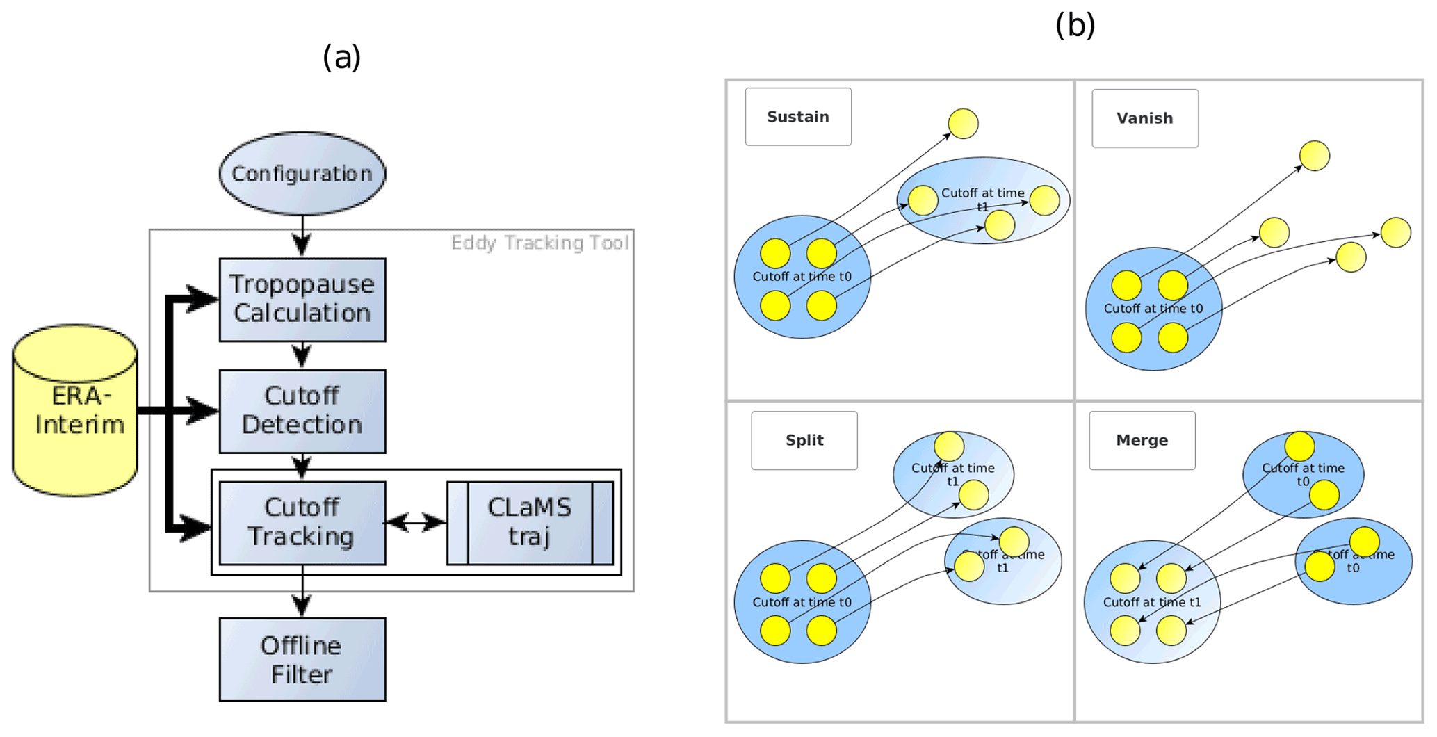
Figure A1 (a) Structure of the PV cutoff tracking tool and (b) a schematic of different evolutions of PV cutoffs. A cutoff can remain, vanish, split, or merge. The blue circles without and with a colour gradient illustrate cutoffs at times of t₀ and t₁. Yellow circles show individual air parcels.

Appendix B: Monthly differences in cutoff transport

Figure B1 shows the cutoff frequency for each month of the JJAS period. In all months, we found high activity over the North Pacific, with the highest activity in JJA and decreased activity in September. Depending on the month, other regions also show high frequencies of cutoffs. The peak over Siberia is the strongest in June and weakens until September. It needs more investigation to estimate how much of this signal can still be related to cutoffs that are transported from Europe in an eastward direction and how much of this signal can be related to the ASMA. The most promising region and time for measurements of transported anticyclonic air masses that cross the tropopause is the North Pacific from July to August.

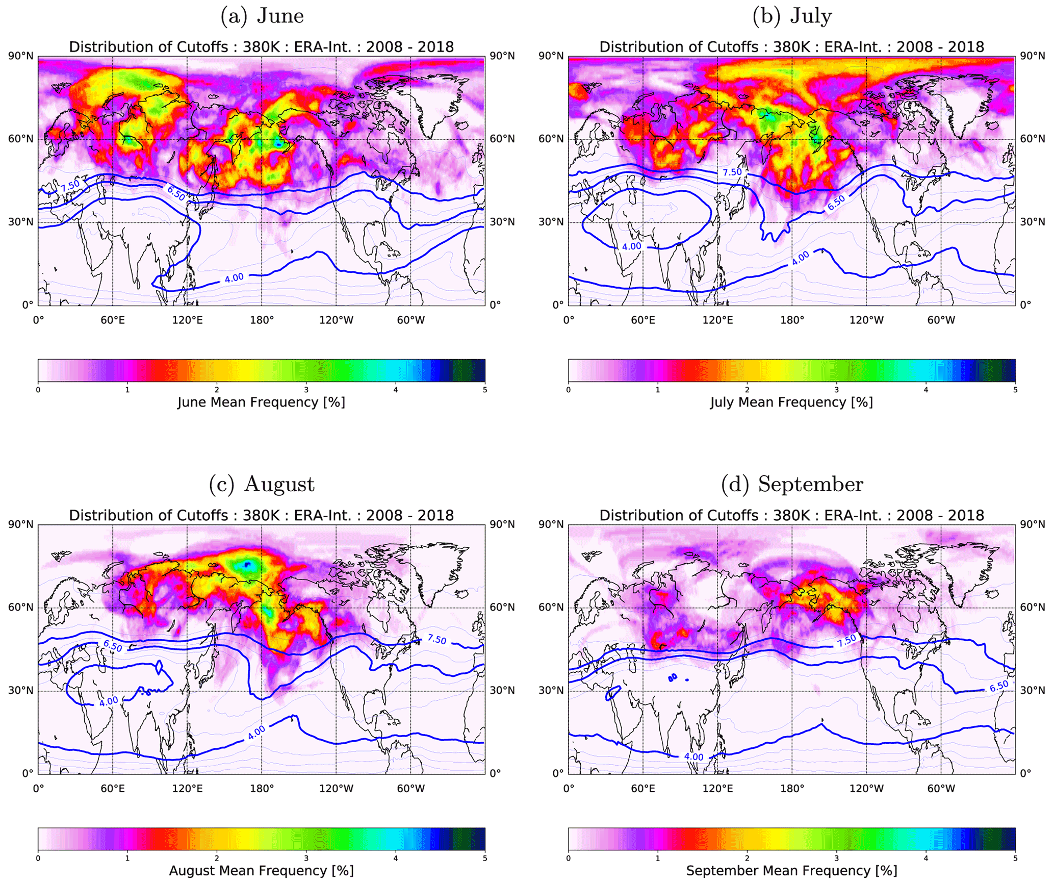
Figure B1 Global climatological frequency distribution of ASMA-related 7.5 PVU cutoffs for each month in JJAS.

Appendix C: Validation of filter via backward calculations

To verify the applied filter method, we initialized air parcel backward trajectories inside filtered cutoffs and analysed whether they indeed originated in the ASMA for the summer monsoon season in 2017. The backward trajectories for 4.0 and 6.5 PVU cutoffs were chosen to have a length of 14 d, and we chose 30 d for 7.5 PVU cutoffs. A length of 14 d is suitable for the 4.0 and 6.5 PVU cutoffs, as the maximum lifetime of those was shown to be around 2 weeks. For 7.5 PVU cutoffs, a trajectory length of 30 d was chosen, as these cutoffs often form in the decay phase of a 6.5 PVU cutoff (see Fig. 1) and, therefore, may exist for up to 14 d longer. To define the contact with the ASMA, we set a rectangular box that corresponds to the climatological position and extent of the ASMA as similarly suggested in other studies (e.g. Garny and Randel, 2016). The box is defined to span the range between longitudes of 20 and 120^∘ E and latitudes of 10 and 50^∘ N. A trajectory is defined to be in contact with the ASMA if it was located within the ASMA box for at least 1 d (four reanalysis time steps). For each cutoff, we calculated the ratio of trajectories that originated in the ASMA. If this ratio was ≥ 0.3 – at least about one-third of the air came from the ASMA – then the cutoff was identified as a cutoff originating in the ASMA. As a result, 93 % of the 4.0 PVU cutoffs, 79 % of the 6.5 PVU cutoffs, and 96 % of the 7.5 PVU cutoffs were identified as being of ASMA origin. The lower frequency for 6.5 PVU compared to 7.5 PVU cutoffs is likely related to the shorter trajectory calculation time of 6.5 PVU cutoffs (14 d vs. 30 d for 7.5 PVU cutoffs) and the related neglection of the longest transport pathways (e.g. to Siberia). In summary, during summer 2017, both the backward trajectory method and the empirical filter method provide very similar results, corroborating the usage of the filter method in this study.

Some limitations of this validation should be noticed. First, the exact definition of the ASMA box can slightly modify the number of trajectories that are related to the monsoon. However, as shown by Garny and Randel (2016), the simplification of a rectangular box versus a more physical PV contour for the ASMA extent does not substantially change the results concerning trajectory origins. Second, backward calculations were limited to the 380 K level; hence, vertical transport was not included. On the considered timescales of a few days to weeks, we also deem this approximation reasonable.