Intricate relations among particle collision, relative motion and clustering in turbulent clouds: computational observation and theory

Considering turbulent clouds containing small inertial particles, we investigate the effect of particle collision, in particular collision–coagulation, on particle clustering and particle relative motion. We perform direct numerical simulation (DNS) of coagulating particles in isotropic turbulent flow in the regime of small Stokes number (St=0.001–0.54) and find that, due to collision–coagulation, the radial distribution functions (RDFs) fall off dramatically at scales r∼d (where d is the particle diameter) to small but finite values, while the mean radial component of the particle relative velocity (MRV) increases sharply in magnitude. Based on a previously proposed Fokker–Planck (drift-diffusion) framework, we derive a theoretical account of the relationship among particle collision–coagulation rate, RDF and MRV. The theory includes contributions from turbulent fluctuations absent in earlier mean-field theories. We show numerically that the theory accurately accounts for the DNS results (i.e., given an accurate RDF, the theory could produce an accurate MRV). Separately, we also propose a phenomenological model that could directly predict MRV and find that it is accurate when calibrated using fourth moments of the fluid velocities. We use the model to derive a general solution of RDF. We uncover a paradox: the past empirical success of the differential version of the theory is theoretically unjustified. We see a further shape-preserving reduction of the RDF (and MRV) when the gravitational settling parameter (S_g) is of order O(1). Our results demonstrate strong coupling between RDF and MRV and imply that earlier isolated studies on either RDF or MRV have limited relevance for predicting particle collision rate.

1 Introduction

The motion and interactions of small particles in turbulence have fundamental implications for atmospheric clouds; specifically, they are relevant for the timescale of rain formation, particularly in warm clouds (Falkovich et al., 2002; Wilkinson et al., 2006; Grabowski and Wang, 2013) (a similar problem also applies to planet formation in astrophysics; Johansen et al., 2007). They are also important for engineers who are designing future, greener combustion engines, as this is a scenario they wish to understand and control in order to increase fuel efficiency (Karnik and Shrimpton, 2012). Cloud particles or droplets, due to their inertia, are known to be ejected from turbulent vortices and thus form clusters – regions of enhanced particle density (Wood et al., 2005; Bec et al., 2007; Saw et al., 2008; Karpińska et al., 2019); this together with droplet collision is of direct relevance for the mentioned applications. Due to the technical difficulty of obtaining extensive and systematic experimental or field data on particle/droplet collision in turbulent cloud, many of the recent studies rely on direct numerical simulation (DNS), examples of which can be found in, e.g., Onishi and Seifert (2016) and Wang et al. (2008), and reference therein. Up until now, we have not had definitive answers to basic questions such as how to calculate the particle collision rate from basic turbulence-particle parameters and what the exact relation between collision and particle clustering and/or motions is, for, as we shall see, our work reveals that collision–coagulation causes profound changes in particle relative velocity statistics and particle clustering, questioning earlier understanding of the problem. The difficulty of this problem is in part related to the fact that turbulence is, even by itself, theoretically virtually intractable due to its nonlinear and complex nature.

The quest for a theory of particle collision in turbulence started in 1956 when Saffman and Turner (1956) derived a mean-field formula for the collision rate of finite-size, inertia-less particles. In another landmark work (Sundaram and Collins, 1997), a general relation among the collision rate (R_c), particle clustering and mean particle relative radial velocity was presented: $R_c/\left(n_{\mathrm{1}}{n}_{\mathrm{2}}V\right)=\mathrm{4}\mathit{\pi }{d}^{\mathrm{2}}g\left(d\right)\langle w_r\left(d\right){\rangle }_{\ast }$, where g(r) is the particle radial distribution function (RDF), w_r is the radial component of relative velocity between two particles, $\langle \cdot {\rangle }_{\ast }$ denotes averaging over particle pairs, 〈w_r(d)〉_∗ is the mean radial component of relative particle velocity (MRV), n_i denotes the global averages of particle number density, V is the spatial volume of the domain and d is the particle diameter. The remarkable simplicity of this finding inspired a “separation paradigm”, which is the idea that one could study the RDF or MRV separately (which is technically easier), and the independent results from the two may be combined to accurately predicts R_c (an idea that we subsequently challenge). Another work of special interest here is the drift-diffusion model by Chun et al. (2005) (hereafter CK theory) (note that there are other similar theories: Balkovsky et al., 2001; Zaichik and Alipchenkov, 2003). The CK theory, derived for non-colliding particles in the limit of a vanishing particle Stokes number, St (a quantity that reflects the importance of the particle's inertia in dictating its motion in turbulence), correctly predicted the power-law form of the RDF (Reade and Collins, 2000; Saw et al., 2008) and has seen remarkable successes over the years, including the accurate account of the modified RDF of particles interacting electrically (Lu et al., 2010) and hydrodynamically (Yavuz et al., 2018).

Here, we first present results on RDF and MRV for particles undergoing collision–coagulation¹. The data are obtained via direct numerical simulation (DNS), which is the gold-standard computational method in terms of accuracy and completeness for solving the most challenging fluid dynamics problem i.e., turbulent flows. It is worth noting that the focus of our work is on the fundamental relationship between collision, RDF and MRV and on highlighting differences from the case with non-colliding particles (Chun et al., 2005). To that end, we have designed the DNS to have an idealized setup similar to what was done in Chun et al. (2005), which would allow us to identify the effects of particle collision–coagulation without doubt. As a result, this limits the direct applicability to real systems (these limitations are detailed in Sect. 4.5).

Analysis of the DNS results is followed by a theoretical account of the relations between collision rate, RDF and MRV, which includes mean-field contributions (Saffman and Turner, 1956; Sundaram and Collins, 1997) and contributions from turbulent fluctuations (absent from earlier theories, Saffman and Turner, 1956; Sundaram and Collins, 1997). The theory is derived from the Fokker–Planck (drift-diffusion) framework first introduced in the CK theory (Chun et al., 2005). We shall see that the main effect of collision–coagulation is the enhanced asymmetry in the particle relative velocity distribution² and that this leads to nontrivial outcomes.

2 Direct numerical simulation (DNS)

To observe how particle collision–coagulation affects RDF and MRV, we performed direct numerical simulation (DNS) of steady-state isotropic turbulence embedded with particles of finite but sub-Kolmogorov size. We solve the incompressible Navier–Stokes equations (Eq. 1) using the standard pseudo-spectral method (Rogallo, 1981; Pope, 2000; Mortensen and Langtangen, 2016) inside a triply periodic cubic box.

$$\begin{array}{ll}{\displaystyle }& {\displaystyle \frac{\partial \mathbf{u}}{\partial t}}+\mathbf{u}\cdot \mathrm{\nabla }\mathbf{u}=-{\displaystyle \frac{\mathrm{1}}{\mathit{\rho }}}\mathrm{\nabla }p+\mathit{\nu }{\mathrm{\nabla }}^{\mathrm{2}}\mathbf{u}+\mathbf{f}(\mathbf{x},t),\\ \text{(1)}& {\displaystyle }& {\displaystyle }\mathrm{\nabla }\cdot \mathbf{u}=\mathrm{0},\end{array}$$

where ρ, p, ν and f are the fluid mass density, pressure, kinematic viscosity and imposed forcing respectively. The velocity field is discretized on a 256³ grid. Aliasing resulting from Fourier transform of truncated series is removed via a $\mathrm{2}/\mathrm{3}$ dealiasing rule (Rogallo, 1981). A statistically stationary and isotropic turbulent flow is achieved by continuously applying random forcing to the lowest wave numbers until the flow's energy spectrum is in steady state (Eswaran and Pope, 1988). Second-order Runge–Kutta time stepping was employed. Further details of such a standard turbulence simulator can be found in, e.g., Pope (2000), Rogallo (1981) and Mortensen and Langtangen (2016). The accuracy of DNS for turbulent flows has been experimentally validated for decades (see, e.g., the compilation of results in Pope, 2000).

Table 1 Values of the parameters in the DNS. (Note that dm denotes decimeters.) From the left, we have the Taylor-scale Reynolds number, kinematic viscosity of the fluid, root-mean-square of fluid velocity, kinetic energy dissipation rate, Kolmogorov length scale and timescale, length of the simulation cube and particle diameters considered. We have introduced d_∗ to represent the specific value $\mathrm{9.49}\times {\mathrm{10}}^{-\mathrm{4}}$ dm (more details in the text). We choose the units of the length scale (timescale) in the DNS to be in decimeters (seconds), such that ν is nearly its typical value in the atmosphere.

Particles in the simulations are advected via a viscous Stokes drag force (Maxey and Riley, 1983):

$$\mathrm{d}\mathbf{v}/\mathrm{d}t=(\mathbf{u}-\mathbf{v})/{\mathit{\tau }}_p,$$

where u and v are the local fluid and particle velocity respectively, and τ_p is the particle inertia response time, defined as ${\mathit{\tau }}_p=\frac{\mathrm{1}}{\mathrm{18}}({\mathit{\rho }}_p/\mathit{\rho }-\mathrm{1})(d^{\mathrm{2}}/\mathit{\nu })$, where ρ_p is the particle mass density, and d is the particle diameter. As mentioned, this work focuses on the fundamental relationship between collision–coagulation, RDF and MRV, as well as on addressing the validity of the theory (to be described). It is thus, beneficial to keep the DNS setting idealized (and in the regime relevant for the theory) for the sake of clarity when interpreting results. To that end, the DNS does not include inter-particle hydrodynamic interactions (HDIs) and gravitational settling, nor does it consider the effects of temperature and humidity variation and phase transitions. Such practice is not uncommon in studies designed to isolate and address fundamental issues related to particles dynamics in turbulence; examples that are closely related to the current setup and/or problem include Sundaram and Collins (1997), Chun et al. (2005), Bec et al. (2007), Salazar et al. (2008), Wang et al. (2008), Woittiez et al. (2009) and Voßkuhle et al. (2013). However, such an approach certainly limits the direct applicability of our results to some realistic problems in the atmosphere; these limitations will be detailed in Sect. 4.5, where a discussion of the effects of gravity and HDI is also given.

In this context, the particle Stokes number, defined as ${\mathit{\tau }}_p/{\mathit{\tau }}_{\mathit{\eta }}$, where τ_η is the Kolmogorov timescale, can be expressed as $\mathit{\text{St}}=\frac{\mathrm{1}}{\mathrm{18}}({\mathit{\rho }}_p/\mathit{\rho }-\mathrm{1})(d/\mathit{\eta }{)}^{\mathrm{2}}$, where η is the Kolmogorov length scale. Time stepping of the particle motion is done using a second-order modified Runge–Kutta method with an “exponential integrator” that is accurate, even for τ_p much smaller than the fluid's time step (Ireland et al., 2013). The particles introduced into the simulation are spherical and are of the same size, the initial number of particles is 10⁷ and they are randomly distributed in space. Particles collide when their volumes overlap and a new particle is formed conserving volume and momentum (Bec et al., 2016). We continuously, randomly, inject new particles so that the system is in a steady state after some time. Statistical analysis is done at steady state on monodisperse particles (i.e., particles with the same St). Experimental validation of the accuracy of such a particle simulation scheme in DNS can be found in Salazar et al. (2008), Saw et al. (2012, 2014) and Dou et al. (2018).

Values of key parameters of the DNS are given in Table 1. Values of other parameters and further details can be found in the Supplement.

3 Elements of the drift-diffusion theory

As described in Chun et al. (2005), in the limit of St≪1, particle motions are closely tied to the fluid velocity and, to leading order, completely specified by the particle position and fluid velocity gradients. We consider the Fokker–Planck equation which is closed and deterministic (see, e.g., Appendix J in Pope, 2000):

$$\begin{array}{}\text{(2)}& {\displaystyle \frac{\partial P}{\partial t}}+{\displaystyle \frac{\partial \left(W_{i}P\right)}{\partial r_i}}=\mathrm{0},\end{array}$$

where $P\equiv P(r_i,t|{\mathrm{\Gamma }}_{ij}\left(t\right))$ is the (per volume) probability density function (PDF) for a secondary particle to be at vector position r_i relative to a primary particle at time t, conditioned on a fixed and known history of the velocity gradient tensor along the primary particle's trajectory Γ_ij(t), and W_i is the mean velocity of secondary particles relative to the primary, under the same condition. Note that W_i is a conditional average, while w_i denotes a realization of relative velocity between two particles.

From this, one could derive an equation for 〈P〉:

$$\begin{array}{}\text{(3)}& {\displaystyle \frac{\partial \langle P\rangle }{\partial t}}+{\displaystyle \frac{\partial }{\partial r_i}}(\langle W_i\rangle \langle P\rangle +\langle W_i{P}^{\prime }\rangle )=\mathrm{0},\end{array}$$

where 〈.〉 implies ensemble averaging over primary particle histories (note that 〈W_r〉≡ unconditional mean of w_r, averaged over all particle pairs, i.e., the MRV). This equation, however, is not closed due to the correlation between the fluctuating terms W_i and $P^{\prime }\equiv P-\langle P\rangle$. The correlation 〈W_iP^′〉 can be written in terms of a drift flux and diffusive flux (detailed derivation is well described in Chun et al., 2005), such that we have

$$\begin{array}{}\text{(4)}& {\displaystyle \frac{\partial \langle P\rangle }{\partial t}}+{\displaystyle \frac{\partial }{\partial r_i}}(q_i^d+q_i^D)+{\displaystyle \frac{\partial (\langle W_i\rangle \langle P\rangle )}{\partial r_i}}=\mathrm{0},\end{array}$$

where the drift flux is

$$\begin{array}{}\text{(5)}& q_i^d=-\underset{-\mathrm{\infty }}{\overset{t}{\int }}〈W_i(\mathbf{r},t){\displaystyle \frac{\partial W_l}{\partial r_l^{\prime }}}({\mathbf{r}}^{\prime },t^{\prime })〉\langle P\rangle ({\mathbf{r}}^{\prime },t^{\prime })\mathrm{d}{t}^{\prime },\end{array}$$

and the diffusive flux is

$$\begin{array}{}\text{(6)}& q_i^D=-\underset{-\mathrm{\infty }}{\overset{t}{\int }}〈W_i(\mathbf{r},t)W_j({\mathbf{r}}^{\prime },t^{\prime })〉{\displaystyle \frac{\partial \langle P\rangle }{\partial r_j^{\prime }}}({\mathbf{r}}^{\prime },t^{\prime })\mathrm{d}{t}^{\prime },\end{array}$$

where r^′ satisfies a characteristic equation: $\partial r_i^{\prime }/\partial t^{\prime }=W_i({\mathbf{r}}^{\prime },t^{\prime })$, with boundary condition $r_i^{\prime }=r_i$ at $t^{\prime }=t$.

Finally we note that since particles are allowed to collide–coagulate in our theory, we use the conventional definition of MRV: $\langle W_r\rangle \equiv \langle w_r{\rangle }_{\ast }$. In some works that consider non-colliding (ghost) particles, the conditional mean $\langle w_r|w_r\le \mathrm{0}{\rangle }_{\ast }$ must be used for the purpose of calculating the mean collision rate, since $\langle w_r{\rangle }_{\ast }=\mathrm{0}$ in isotropic turbulence (Chun et al., 2005).

4 DNS results, theory and discussion

We compute the RDF via $g\left(r\right)=N_{\text{pp}}\left(r\right)/\left[\frac{\mathrm{1}}{\mathrm{2}}N\right(N-\mathrm{1})\mathit{\delta }{V}_r/V]$, where N_pp(r) is the number of particle pairs found to be separated by distance r, and δV_r is the volume of a spherical shell of radius r and infinitesimal thickness δr.

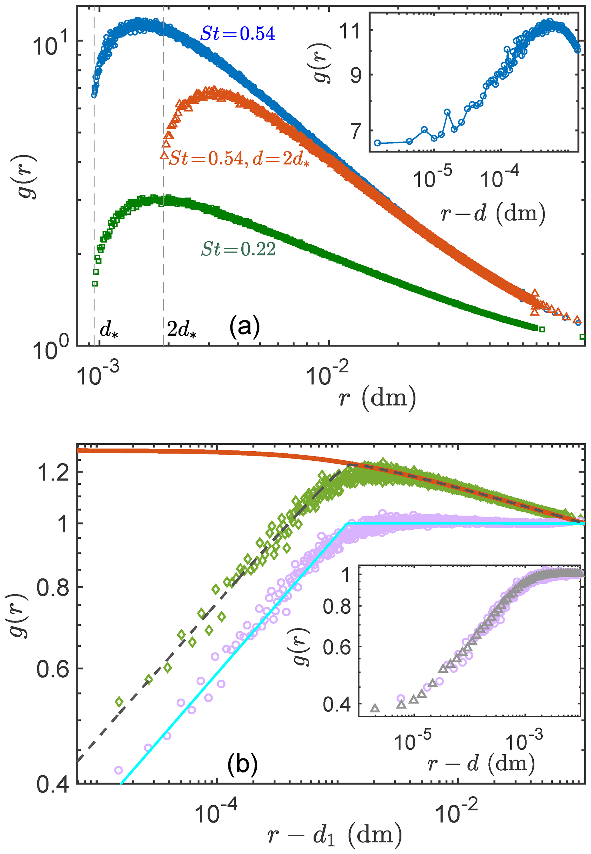
Figure 1 RDFs (g(r)) of particles that coagulate upon collision. (a) g(r) for various cases of Stokes numbers and particle diameters (d). □: St=0.22, $d=d_{\ast }$, ◦: St=0.54, $d=d_{\ast }$, △: St=0.54, $d=\mathrm{2}{d}_{\ast }$. All g(r) values drop off exponentially when r→d (details in text). Inset: g(r) versus r−d for the ◦ case. This exemplifies the fact that ${lim}_{r\to d}g\left(r\right)$ is nonzero. (b) RDFs versus r−d₁ (where d₁=0.99d) for the case of St=0.054, $d=d_{\ast }$. ◇: the raw DNS-produced RDF (g_DNS(r)). Red line: power-law fit to g_DNS(r) (i.e., the ◇ plot) in the large r regime (the fit result is 0.890r^−0.0535). It is equivalent to g_s(r) in the ansatz g_a(r)=g₀(r)g_s(r); i.e., it is the expected RDF for non-colliding particles under the same conditions. ◦: the compensated RDF, i.e., $g_{\text{DNS}}\left(r\right)/g_s\left(r\right)$ (note that g_s(r) is the red line described earlier); this essentially gives us g₀(r), which may be understood as a “modulation” on the RDF due to collision–coagulation. Cyan line: two-piece power-law fits to the compensated RDF (the ◦ plot) in the small and large r−d₁ regimes respectively (fit results: 4.17(r−d₁)^0.212, $\mathrm{1.00}(r-d_{\mathrm{1}}{)}^{-\mathrm{2}\times {\mathrm{10}}^{-\mathrm{4}}}$); this is an estimate for g₀(r). Dashed black line: g₀(r)g_s(r), (cyan line × red line); this shows that the ansatz accurately reproduces g_DNS(r). Inset: RDFs versus r−d. ◦: compensated g(r) for St=0.054, $d=d_{\ast }$, equivalent to the ◦ plot in the panel's main figure; △: compensated RDF for case St=0.001, $d=d_{\ast }$, i.e., finite size, almost zero St particles (in this case, the compensated and raw RDFs are the identical). This inset suggests that g₀(r) has negligible St dependence.

Figure 1 shows the RDFs obtained for monodisperse particles of various Stokes numbers and sizes. Two cases (St=0.22 and 0.54) are shown in panel a, and two more (St=0.054 and 0.001) are shown in panel b. In this work, we focus on the smaller values of St since the theory which we shall consider is also only applicable in the St≪1 regime. However, we have included the St=0.54 case to demonstrate that the observations to be described also extends to finite St. In all cases, except one, the particles are of the same size $d=d_{\ast }$, where d_∗ represents the specific value of $d_{\ast }=\mathrm{9.49}\times {\mathrm{10}}^{-\mathrm{4}}$ dm, chosen so that the particle sizes are about O(0.1) times the Kolmogorov scale (η), thus allowing us to still observe a regime (3d≲r≲30η) of power-law RDFs. To shows the effect of changing particle size, panel a also includes a case of $\mathit{\text{St}}=\mathrm{0.54},d=\mathrm{2}{d}_{\ast }$ for comparison. Looking at panel a, apart from the apparent power-law behavior of the RDFs at intermediate values of r, the most striking feature of these RDFs for colliding–coagulating particles is that they fall off dramatically in the r∼d regime. This is very different from what was seen in earlier studies of non-colliding particles, where g(r) are simple power laws (Chun et al., 2005; Saw et al., 2008). We also see that as r approaches d, the steepness of the curve (see, e.g., the blue circles) increases as g(r) drops off; this and the fact that the abscissa is logarithmic implies that $\partial g/\partial r$ is increasing exponentially in the process. As a consequence, it is difficult to discern from these plots if the limit of g(r) at particle contact (r→d) is still nonzero. This is an important question as ${lim}_{r\to d}\left[g\right(r\left)\right]=\mathrm{0}$ implies that the mean-field formula of Sundaram and Collins (1997) has zero contribution towards R_c; i.e., the collision rate is solely due to turbulent fluctuations. It is only by re-plotting g(r) versus r−d (see insets in Fig. 1) and using a remarkable resolution that is 10³ finer than d that we see a convincing trend supporting a finite g(r→d). Also clear in panel a is the observation that with changing particle size (d), the location of the sharp fall-off merely shifts to where the new value of d is.

The strong effect of particle collision on the RDF (also on MRV as we shall see later) challenges the validity of the separation paradigm. We note that similar fall-off of RDF was previously observed (Sundaram and Collins, 1997), but a complete analysis and theoretical understanding were lacking. Also, a study on multiple collisions (Voßkuhle et al., 2013) had hinted at the potential problem with the separation paradigm.

Another observation is that in the power-law regime (3d≲r≲30η), the RDFs appear (as expected) as straight lines with slopes (i.e., power-law exponents) that increase with St and are numerically consistent with those found for non-colliding particles (see, e.g., Saw et al., 2012).

4.1 Theoretical account via drift-diffusion theory

To theoretically account for the new findings, we make some derivations that are partially similar to the ones in Chun et al. (2005) but under a new constraint due to coagulations: at contact (r=d), the radial component of the particle relative velocities can not be positive³, while with increasing r the constraint is gradually relaxed. The first consequence of this is that the distribution of the radial component of the relative particle velocity (W_r) is highly asymmetric at r≈d; i.e., the PDFs of positive W_r values are very small (this constitutes the “enhanced asymmetry” mentioned earlier). Thus for r≈d, 〈W_r〉 must be negative. In Sect. 3, we showed that in the St≪1 limit, one could derive a master equation (Eq. 4), reproduced here for clarity:

$${\displaystyle \frac{\partial \langle P\rangle }{\partial t}}+{\displaystyle \frac{\partial }{\partial r_i}}(q_i^d+q_i^D)+{\displaystyle \frac{\partial (\langle W_i\rangle \langle P\rangle )}{\partial r_i}}=\mathrm{0},$$

where $q_i^d$ is the drift flux (of probability due to turbulent fluctuation) defined in Eq. (5), and $q_i^D$ is the diffusive flux defined in Eq. (6).

We then expand W_i, $\partial W_l/\partial r_l$ and (consequentially) the fluxes as perturbation series with St as the small parameter (details in the Supplement or Chun et al., 2005). The coagulation constraint affects the values of the coefficients of these series. For the drift flux, the leading-order terms (in powers of St) are

$$\begin{array}{}\text{(7)}& q_i^d=-\langle P\rangle \left(\mathbf{r}\right)r_k\underset{-\mathrm{\infty }}{\overset{t}{\int }}\left[a_{ik}^{\left(\mathrm{1}\right)}\mathit{\text{St}}+a_{ki}^{\left(\mathrm{2}\right)}{\mathit{\text{St}}}^{\mathrm{2}}\right]\mathrm{d}{t}^{\prime },\end{array}$$

with $a_{ik}^{\left(\mathrm{1}\right)}={\mathit{\tau }}_{\mathit{\eta }}\langle {\mathrm{\Gamma }}_{ik}\left(t\right){\mathrm{\Gamma }}_{lm}\left(t^{\prime }\right){\mathrm{\Gamma }}_{ml}\left(t^{\prime }\right)\rangle$ and $a_{ki}^{\left(\mathrm{2}\right)}={\mathit{\tau }}_{\mathit{\eta }}^{\mathrm{2}}\langle {\mathrm{\Gamma }}_{ij}\left(t\right){\mathrm{\Gamma }}_{jk}\left(t\right){\mathrm{\Gamma }}_{lm}\left(t^{\prime }\right){\mathrm{\Gamma }}_{ml}\left(t^{\prime }\right)\rangle$, where Γ_ij is the ijth component of the fluid's velocity gradient tensor at the particle position (the a_ik values are thus related to two time correlations of moments of velocity gradients; Chun et al. (2005) showed that $a_{ik}^{\left(\mathrm{2}\right)}\propto \stackrel{\mathrm{‾}}{S^{\mathrm{2}}}-\stackrel{\mathrm{‾}}{R^{\mathrm{2}}}$, where $(\stackrel{\mathrm{‾}}{S^{\mathrm{2}}},\stackrel{\mathrm{‾}}{R^{\mathrm{2}}})$ denotes the average fluid (strain rate tensor, rotation rate tensor) squared at particle positions). As explained earlier, coagulation constraint causes the PDF of relative particle velocities to become highly asymmetric for r∼d; thus $a_{ik}^{\left(\mathrm{1}\right)}$ is nonzero at this scale. This is very different from the case of non-colliding particles (Chun et al., 2005), where $a_{ik}^{\left(\mathrm{1}\right)}$ is always zero due to statistical isotropy. Under the constraint, DNS gives ${\int }_{-\mathrm{\infty }}^t{a}_{ik}^{\left(\mathrm{1}\right)}\mathrm{d}{t}^{\prime }\approx -\mathrm{0.18}$ s⁻¹ and ${\int }_{-\mathrm{\infty }}^t{a}_{ki}^{\left(\mathrm{2}\right)}\mathrm{d}{t}^{\prime }\approx \mathrm{2.45}$ s⁻¹ (more in the Supplement). Thus for r∼d, the drift flux is negative for large St but becomes positive⁴ when St is below the value of ≈0.07; and in the limit of St→0, it is dominated by the first term in Eq. (7).

The term $q_i^D$ is a “nonlocal” diffusion caused by fluctuations and can be estimated using a model that assumes the particle relative motions are due to a series of random uniaxial straining flows (Chun et al., 2005). Chun et al. (2005) showed that, generally, $q_i^D$ has an integral form (due to non-locality), and only in the special case where g(r) is a power law may it be cast into a differential form (similar to a local diffusion). In view of the nontrivial g(r) observed here, we must proceed with the integral form:

$$\begin{array}{ll}{\displaystyle }{q}_r^D& {\displaystyle }=c_{\mathit{\text{st}}}r\int \mathrm{d}\mathrm{\Omega }\underset{\mathrm{0}}{\overset{\mathrm{\infty }}{\int }}\mathrm{d}{t}_{f}F\left(t_f\right)\\ {\displaystyle }& {\displaystyle }\times \underset{d/r}{\overset{\mathrm{\infty }}{\int }}\mathrm{d}{R}_{\mathrm{0}}{R_{\mathrm{0}}}^{\mathrm{2}}\langle P\rangle \left(r{R}_{\mathrm{0}}\right)f_I(R_{\mathrm{0}},\mathit{\mu },t_f),\end{array}$$

where $R_{\mathrm{0}}\equiv r_{\mathrm{0}}/r$, with r₀ as the initial separation distance of a particle pair before a straining event. F is the probability density function for the duration of each event, f_I is determined by relative prevalence of extensional versus compressional strain events (more details in the Supplement or Chun et al., 2005) and Ω is the solid angle for the axis of the straining flow. Note that due to coagulation, the R₀ integration starts from $d/r$. We differ crucially from the CK theory via the introduction of the (positive) factor c_st, which can be shown to be equal to $\left|c_{\mathrm{1}}\right|$, where c₁ is the power-law exponent of the RDF the particles would have assuming they are non-colliding (details in the Supplement).

By definition, g(r)≡α〈P〉. Periodic boundaries in our DNS imply that α=V (more in the Supplement). Using this and the fact that the problem only has radial (r) dependence, we rewrite Eq. (4) as

$$\begin{array}{}\text{(8)}& r^{\mathrm{2}}{\displaystyle \frac{\partial g(r,t)}{\partial t}}+{\displaystyle \frac{\partial }{\partial r}}\left[r^{\mathrm{2}}\mathit{\alpha }(q_i^d+q_i^D)+r^{\mathrm{2}}\langle W_r\rangle g(r,t)\right]=\mathrm{0},\end{array}$$

where the content inside [.] gives the total flux. For a system in steady state, the first term in Eq. (8) is zero, and upon integrating with limits [d,r], we have

$$\begin{array}{ll}{\displaystyle }{c}_{\mathit{\text{st}}}{r}^{\mathrm{3}}\int \mathrm{d}\mathrm{\Omega }& {\displaystyle }\underset{\mathrm{0}}{\overset{\mathrm{\infty }}{\int }}\mathrm{d}{t}_{f}F\left(t_f\right)\underset{d/r}{\overset{\mathrm{\infty }}{\int }}\mathrm{d}{R}_{\mathrm{0}}{R}_{\mathrm{0}}^{\mathrm{2}}g\left(r{R}_{\mathrm{0}}\right)f_I(R_{\mathrm{0}},\mathit{\mu },t_f)\\ \text{(9)}& {\displaystyle }& {\displaystyle }+g\left(r\right)\left[r^{\mathrm{2}}\langle W_r\rangle -A_{\mathit{\tau }}{r}^{\mathrm{3}}\right]=-R_c^{*},\end{array}$$

where we have identified the total flux at contact (r=d) as the negative of the (always positive) normalized collision rate $R_c^{*}\equiv R_c/\left(\mathrm{4}\mathit{\pi }\left[N\right(N-\mathrm{1})/\mathrm{2}]/V\right)$, and comparing with Eq. (7), we see that

$$\begin{array}{}\text{(10)}& A_{\mathit{\tau }}\equiv \mathit{\text{St}}\underset{-\mathrm{\infty }}{\overset{t}{\int }}{a}_{ik}^{\left(\mathrm{1}\right)}\mathrm{d}{t}^{\prime }+{\mathit{\text{St}}}^{\mathrm{2}}\underset{-\mathrm{\infty }}{\overset{t}{\int }}{a}_{ki}^{\left(\mathrm{2}\right)}\mathrm{d}{t}^{\prime },\end{array}$$

with the specific values of the t^′ integrals already given above. For clarity, we reiterate that on the left side of Eq. (9), we have the diffusive flux ($q_r^D$), mean-field flux (r²g(r)〈W_r〉) and drift flux ($q_r^d$), while on the right, the total flux is given in terms of the normalized collision rate ($R_c^{*}$). We note that this equation embodies the full relationship among RDF, MRV and collision rate.

4.2 Ansatz and accuracy of the theory

Simple analytical solutions to Eq. (9) may be elusive due to its integral nature (a consequence of the non-local diffusive flux). However, one could gain insights into it and test its accuracy via numerical solutions. To that end, we begin with a simple ansatz for g(r), then we curve-fit the ansatz to the DNS-produced RDF (g_DNS(r)). This enables us to, firstly, verify that the ansatz could accurately represent g_DNS(r) and, secondly, to obtain a “calibrated” ansatz that is a numerically accurate representation of g_DNS(r). We then show that Eq. (9), supplied with the calibrated ansatz, could numerically predict 〈W_r〉(r) (i.e., MRV) that agrees well with the DNS-produced MRV. In short, we will show that given a “correct” g(r), Eq. (9) produces the “correct” 〈W_r〉(r).

The ansatz has the form g_a(r)=g₀(r)g_s(r), with $g_s\left(r\right)=c_{\mathrm{0}}{r}^{-c_{\mathrm{1}}}$, i.e., the RDF form for non-colliding particles (Chun et al., 2005) under the same conditions. As a first-order analysis, we let g₀, which embodies the effects of collision, take the simplest form that could still capture the main features of the RDFs seen in Fig. 1. Specifically, we let $g_{\mathrm{0}}\left(r\right)=c_{\mathrm{00}}(r-d_{\mathrm{1}}{)}^{c_{\mathrm{10}}}$, where c₀₀(r) and c₁₀(r) are each piecewise constant quantities that switch from their small r to large r values at a crossover-scale r_c (of the order of d); i.e., g₀ is a two-piece power law of r−d₁. (Note that our earlier finding of $g(r\to d)>\mathrm{0}$ implies that d₁<d.)

From a given DNS-produced RDF (g_DNS(r)), we first obtain a calibrated g_s by fitting $c_{\mathrm{0}}{r}^{-c_{\mathrm{1}}}$ to g_DNS(r) in the power-law regime d≪r≲10η (see the red line in Fig. 1b). Next, we compute the DNS estimate of g₀ via $g_{\mathrm{0}}^{\text{DNS}}=g_{\text{DNS}}\left(r\right)/g_s\left(r\right)$, which is essentially a compensated RDF (see the ◦ plot in Fig. 1b). To get a calibrated g₀, we then fit the general form of g₀ given above to $g_{\mathrm{0}}^{\text{DNS}}$ (see the cyan line in Fig. 1b; note that each time, two pieces of power laws are fitted to one $g_{\mathrm{0}}^{\text{DNS}}$, and r_c results naturally from the intersection of the two). Figure 1b shows the calibrated ansatz for the case of St=0.054 and verifies its accuracy (the red line is g_s(r), the cyan line is g₀(r) and the dashed black line (g₀⋅g_s) accurately reproduces g_DNS(r)). The inset in Fig. 1b shows that $g_{\mathrm{0}}^{\text{DNS}}\left(r\right)$ (i.e., $g_{\text{DNS}}\left(r\right)/g_s\left(r\right)$) is roughly St-independent for St≪1.

Next, we numerically evaluate the integral in the first term of Eq. (9). The St≪1 assumption allows us to approximate g(r,St) inside the integral by its zero-St cousin $g(r,\mathit{\text{St}}\to \mathrm{0})$ (Chun et al., 2005). In practice, we replace g(r,St) with the ansatz fitted to the DNS result of $g(r,\mathit{\text{St}}=\mathrm{0.001})$. Next, we use the DNS data to estimate A_τ and compute $R_c^{*}$ and c_st (for this case, DNS gives $R_c^{*}=\mathrm{9.69}\times {\mathrm{10}}^{-\mathrm{10}}{\mathrm{dm}}^{\mathrm{3}}{\mathrm{s}}^{-\mathrm{1}}$; $c_{\mathit{\text{st}}}=\left|c_{\mathrm{1}}\right|$ as mentioned earlier). Finally we use Eq. (9) to predict 〈W_r〉(r).

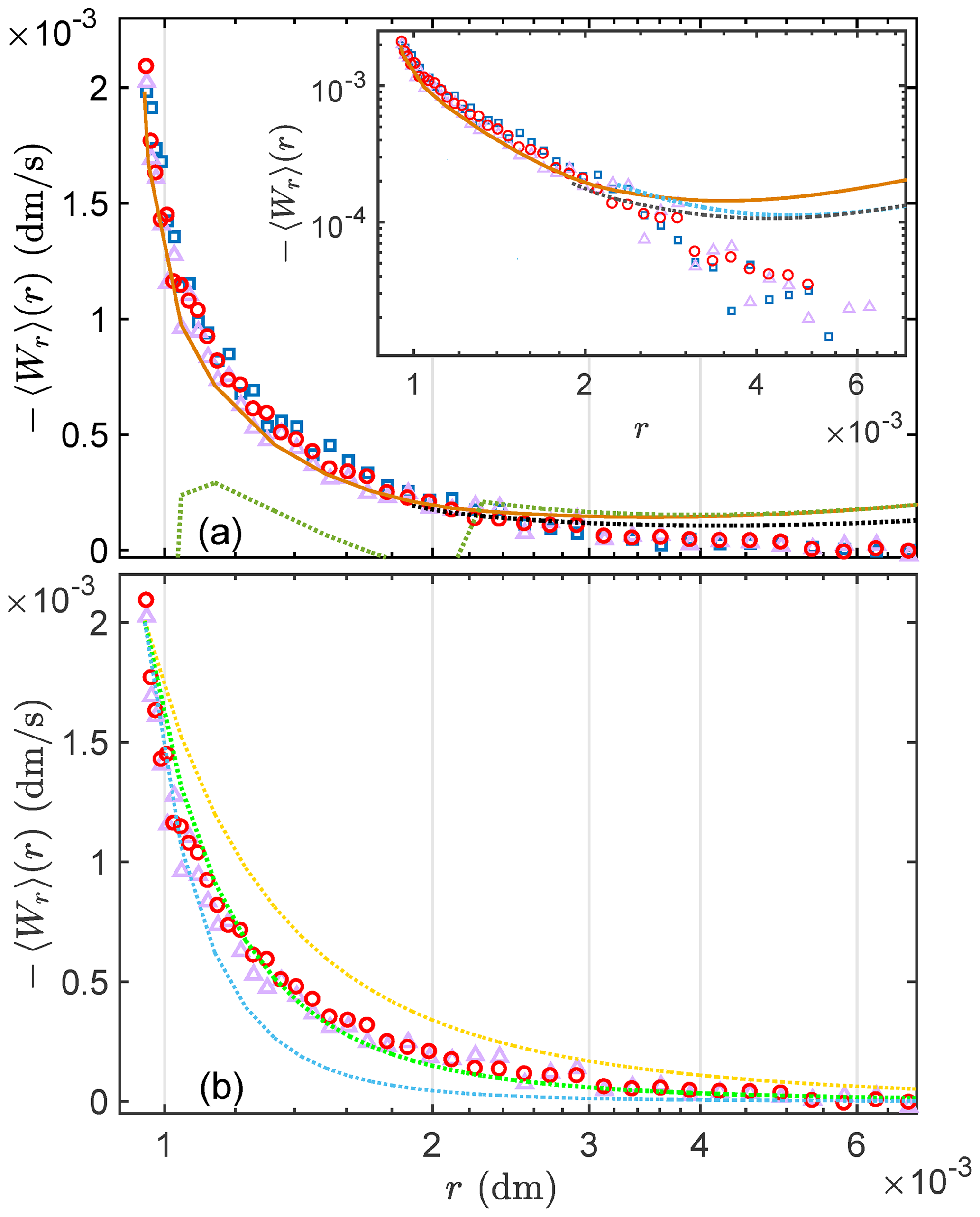
Figure 2 Mean radial component of relative velocity (MRV) for particles of specific Stokes numbers and some theoretic numerical predictions. (a) Symbols are DNS results with △: St=0.001; ◦: St=0.054; □: St=0.11. The lines are the numerical predictions by the theories (Eqs. 9 or 13) using the ansatz (details in text). Orange line: $\langle W_r{\rangle }_{r\sim d,\mathit{\text{St}}=\mathrm{0.054}}^{\text{theory}}$, i.e., the numerical prediction via the integral version of the theory (Eq. 9) for the small r regime (r∼d). Black line: $\langle W_r{\rangle }_{r\gg d,\mathit{\text{St}}=\mathrm{0.054}}^{\text{theory}}$, same as the previous but for the large r regime (r≫d). Green line: prediction of the differential version of the theory (Eq. 13) for the r∼d regime. Inset: a repeat of the main figure in log–log axes. Exception: cyan line is the prediction of the differential version of the theory but for the r≫d regime. (b) MRV compared with predictions via the phenomenological model of particle approach angles (Eqs. 11 and 12). DNS results: △: St=0.001; ◦: St=0.054. Dotted lines are model predictions of 〈W_r〉_St=0 using Eqs. (11) and (12) with variance K obtained by matching the model's and DNS's transverse-to-longitudinal ratio of structure functions (TLR) of a certain order (from the top: yellow line – order 2, green line – order 4, cyan line – order 6).

Comparison of the predicted 〈W_r〉(r) with the values obtained directly from the DNS is shown in Fig. 2. The prediction shown was made for the case of St=0.054, to be compared with its DNS counterpart (the ◦ symbols). (We also show the DNS result for St=0.001 and 0.11 to highlight an observation that 〈W_r〉(r) is almost St-independent in this small St regime.) We showed earlier that for r∼d, A_τ is given by Eq. (10). However, as stated earlier, as r increases, the (statistical) asymmetry induced by collision–coagulation gradually becomes subdominant to the isotropy of turbulent fluctuation. Statistical isotropy implies $a_{ik}^{\left(\mathrm{1}\right)}=\mathrm{0}$ (Chun et al., 2005), a fact our DNS data confirm. Thus, for r≫d, A_τ equals the order St² term in Eq. (10), exactly the same as the results of Chun et al. (2005) for non-colliding particles. For this reason, we show two versions of the prediction: $\langle W_r{\rangle }_{r\sim d}^{\text{theory}}$ and $\langle W_r{\rangle }_{r\gg d}^{\text{theory}}$, which are respectively obtained by setting A_τ to its small r and large r limits ($-\mathrm{2.6}\times {\mathrm{10}}^{-\mathrm{3}}$ s⁻¹, $\mathrm{7.1}\times {\mathrm{10}}^{-\mathrm{3}}$ s⁻¹) respectively. The agreement between DNS and the predictions is noteworthy, especially for small r. At r≈2d, the DNS result shows a weak tendency to first follow the upward trend of $\langle W_r{\rangle }_{r\sim d}^{\text{theory}}$ and then drops off significantly at r≳2.5d. The latter is consistent with the fact that $\langle W_r{\rangle }_{r\gg d}^{\text{theory}}$ is below $\langle W_r{\rangle }_{r\sim d}^{\text{theory}}$, but the drop is sharper than predicted.

4.3 Phenomenological model of MRV

Alternatively, Eq. (9) may be solved for the correct g(r), if 〈W_r〉 is given. As we are assuming St≪1, particle velocity statistics may be approximated by their fluid counterparts (Chun et al., 2005); i.e., we may replace 〈W_r〉 with 〈W_r〉_St=0, the latter being the MRV of fluid particles. Hence, if 〈W_r〉_St=0 is known, it may be used, together with Eq. (9), to predict RDF of any finite but small St. Figure 2a shows that 〈W_r〉_St>0 from the DNS do not change significantly for $\mathit{\text{St}}\in [\mathrm{0.001},\mathrm{0.1}]$, supporting this approach⁵.

Here we provide a simple, first-order model for 〈W_r〉_St=0. We limit ourselves to the regime of small particles (d≪η) and anticipate that 〈W_r〉 is non-trivial (nonzero) only for r∼d, a fact observable in Fig. 2a. We also assume that the relative trajectories of particles are rectilinear at such small scales. The coagulation constraint then implies that: in the rest frame of a particle (call it P1), a second particle nearby must move in such a way that the angle (θ) between its relative velocity and relative position (seen by P1) must satisfy ${\sin }^{-\mathrm{1}}(d/r)\le \mathit{\theta }\le \mathit{\pi }$, under the convention of ${\sin }^{-\mathrm{1}}\left(x\right)\in [-\frac{\mathit{\pi }}{\mathrm{2}},\frac{\mathit{\pi }}{\mathrm{2}}]$ (more in the Supplement). We can thus write (by treating negative and positive w_r separately, applying the K41 theory (Kolmogorov, 1941) and the bounds on θ, details in the Supplement), for St≪1, that

$$\begin{array}{ll}{\displaystyle }\langle W_r\rangle & {\displaystyle }\equiv \langle w_r{\rangle }_{\ast }=p_{\text{–}}\langle w_r|w_r<\mathrm{0}{\rangle }_{\ast }+p_{\text{+}}\langle w_r|w_r\ge \mathrm{0}{\rangle }_{\ast }\\ \text{(11)}& {\displaystyle }& {\displaystyle }\approx -p_{\text{–}}{\mathit{\xi }}_{\text{–}}r+p_{\text{+}}{\mathit{\xi }}_{\text{+}}r\left[\mathrm{1}+{\displaystyle \frac{{\int }_{{\mathit{\theta }}_m}^{\mathrm{0}}{P}_{\mathit{\theta }}^{+}\left({\mathit{\theta }}^{\prime }\right)\cos \left({\mathit{\theta }}^{\prime }\right)\mathrm{d}{\mathit{\theta }}^{\prime }}{{\int }_{\mathrm{0}}^{\frac{\mathit{\pi }}{\mathrm{2}}}{P}_{\mathit{\theta }}^{+}\left({\mathit{\theta }}^{\prime }\right)\cos \left({\mathit{\theta }}^{\prime }\right)\mathrm{d}{\mathit{\theta }}^{\prime }}}\right],\end{array}$$

where $\langle .{\rangle }_{\ast }$ denotes averaging over particle pairs, p₊ (p₋) is the probability of a realization of w_r being positive (negative), and $P_{\mathit{\theta }}^{+}$ is a conditional PDF such that $P_{\mathit{\theta }}^{+}\equiv P\left(\mathit{\theta }|w_r\ge \mathrm{0}\right)\equiv P\left(\mathit{\theta }|\mathit{\theta }\in [\mathrm{0},\frac{\mathit{\pi }}{\mathrm{2}}]\right)$, θ_m is the lower bound of θ described above. For a first-order account, we neglect skewness in the distribution of particle relative velocities and set $p_{\pm }=\mathrm{0.5}$. Following Kolmogorov (1941), we have set $\langle w_r|w_r<\mathrm{0}{\rangle }_{\ast }={\mathit{\xi }}_{\text{–}}r$, where ${\mathit{\xi }}_{\pm }=C_s\sqrt{\mathit{\epsilon }/\left(\mathrm{15}\mathit{\nu }\right)}$, (C_s is a Kolmogorov constant, we found C_s=0.76 by matching ξ_–r to the first-order fluid velocity structure-function from the DNS).

A simple phenomenological model for P(θ) may be constructed using the (statistical) central-limit theorem by assuming that the angle of approach θ at any time is the sum of many random-incremental rotations in the past, thus we write

$$\begin{array}{}\text{(12)}& P\left(\mathit{\theta }\right)=N\exp \left[K\cos \right(\mathit{\theta }-{\mathit{\mu }}_{\mathit{\theta }}\left)\right]\sin \left(\mathit{\theta }\right),\end{array}$$

where Nexp […] is the circular normal distribution, i.e., analog of Gaussian distribution for angular data; sin (θ) results from integration over azimuthal angles (ϕ). We set ${\mathit{\mu }}_{\mathit{\theta }}=\frac{\mathit{\pi }}{\mathrm{2}}$ (neglect skewness in fluid's relative velocity PDF) and obtain K by matching the transverse to longitudinal ratio of structure functions (TLR) of the particle relative velocities with the ones via the DNS data; N is determined via normalization of P(θ). Figure 2b shows the 〈w_r〉_∗ derived via Eqs. (11) and (12), using K calibrated with TLR of second-, fourth-, and sixth-order structure functions respectively. The results have a correct qualitative trend of vanishing values at large r that increase sharply as r approaches d, with the fourth-order's result giving the best agreement with DNS. Currently we do not have a satisfactory rationale to single out the fourth order. The TLR of different orders giving differing results may imply that our first-order model may be incomplete, possibly due to over-simplification in Eq. (12) or to the inaccuracy of the rectilinear assumption ($d/\mathit{\eta }$ in the DNS may be insufficiently small).

4.4 Differential version of the theory, its validity and its solution

We now discuss an important but precarious theoretical issue. Chun et al. (2005) clearly showed that the non-local diffusion ($q_r^D$) may only be converted from its general integral form into a differential version when the underlying RDF is a simple power law. However, Lu et al. (2010) and Yavuz et al. (2018), working in two very different scenarios, found that their predictions using the differential form of the theory agree well with experiments, even when the RDFs involved were clearly not power laws. We shall attempt to remedy this apparent paradox in future work. To examine how well this albeit unjustified method works here, we recast Eq. (9) into its differential form (Chun et al., 2005):

$$\begin{array}{}\text{(13)}& -{\mathit{\tau }}_{\mathit{\eta }}^{-\mathrm{1}}{B}_{nl}{r}^{\mathrm{4}}{\displaystyle \frac{\partial g}{\partial r}}+g\left(r\right)[r^{\mathrm{2}}\langle W_r\rangle -A_{\mathit{\tau }}{r}^{\mathrm{3}}]=-R_c^{*},\end{array}$$

where B_nl=0.0397 (this value is computed from our DNS), and B_nl is expected to depend on flow characteristics, e.g., R_λ and τ_η (more in the Supplement). Using Eq. (13), the same g_sg₀ ansatz, we make another prediction for 〈W_r〉_St=0.054, which is plotted in Fig. 2a (dashed green line). This prediction is far from the DNS at r∼d but performs as well as the integral version at r≫d (the jump in the curve is just an artifact from the kink in the ansatz).

One advantage of Eq. (13) is that it allows for a general solution, which we now give, assuming 〈W_r〉 is given by Eqs. (11) and (12):

$$\begin{array}{}\text{(14)}& g\left(r\right)={\displaystyle \frac{\mathrm{1}}{\mathit{\beta }\left(r\right)}}\left[\int \mathit{\beta }\left(r\right)q\left(r\right)\mathrm{d}r+C\right],\end{array}$$

with $q\left(r\right)=R_c^{*}{\mathit{\tau }}_{\mathit{\eta }}/\left(B_{nl}{r}^{\mathrm{4}}\right)$, $\mathit{\beta }\left(r\right)=\exp \left[\int p\left(r\right)\mathrm{d}r\right]$ and $p\left(r\right)=\left[A_{\mathit{\tau }}r-\langle w_r{\rangle }_{\ast }\right]{\mathit{\tau }}_{\mathit{\eta }}/\left(B_{nl}{r}^{\mathrm{2}}\right)$ (more in the Supplement).

4.5 Effects of gravity and other limitations

Thus far, we have not considered the effects of gravity on the particles. Here we provide a glimpse into the role of gravity (a detailed analysis is beyond the scope of the present study). In keeping with the scope of current work, we restrict ourselves to the case of monodisperse particles only. For this, we rerun the DNS cases of St=0.054 and 0.54 with gravity (to be compared with the zero-gravity case). The new particle advection equation is $\mathrm{d}\mathbf{v}/\mathrm{d}t=(\mathbf{u}-\mathbf{v})/{\mathit{\tau }}_p+\mathit{g}$ (all other details of the DNS remain unchanged). We choose to have the particle settling parameter $S_g\equiv {\mathit{\tau }}_{p}g/u_{\mathit{\eta }}$ (where u_η is the Kolmogorov velocity scale) be in the range O(0.1)−O(1) (this is achieved by letting $\left|\mathit{g}\right|=\mathrm{10}$ dm s⁻²). As a result, the range of S_g and St explored here is well aligned with measured values in natural clouds (Siebert et al., 2010). For the case of St=0.054 (S_g=0.49), we find no discernible difference for both RDF and MRV between the “with gravity” and zero-gravity results (corresponding figures in the Supplement). For the St=0.54 (S_g=4.9) case, Fig. 3 shows the effects of gravity on the RDF and MRV. We see that the slope (exponent of g(r) in the range $d\ll r<\mathrm{20}\mathit{\eta }$) of the RDF in the gravitational case is reduced by about 15 % compared to the zero-gravity case (S_g=0). However, the shape of the RDF in the collision regime (r∼d) is approximately preserved, suggesting that a construct of the form g_collision×g_gravity may be a good first-order model for the full RDF (close examination of the compensated RDFs gives substantial support for this idea, details in the Supplement). These observations imply that as S_g increases from O(0.1) to O(1), the effects of gravity on RDF grow from negligible to significant but not dominant; the main effect is the reduction of the exponent while the collision-related “modulation” (g_collision) remains largely intact. The inset of Fig. 3 shows that the MRV is also weakened by gravity, though the statistical noise limits the strength of this conclusion. Lastly, it is worth noting that in the complementary DNS by Woittiez et al. (2009) that included gravity but not actual collisions, a much stronger gravitational effect was found on the statistics of bidisperse particles relative to the monodisperse case.

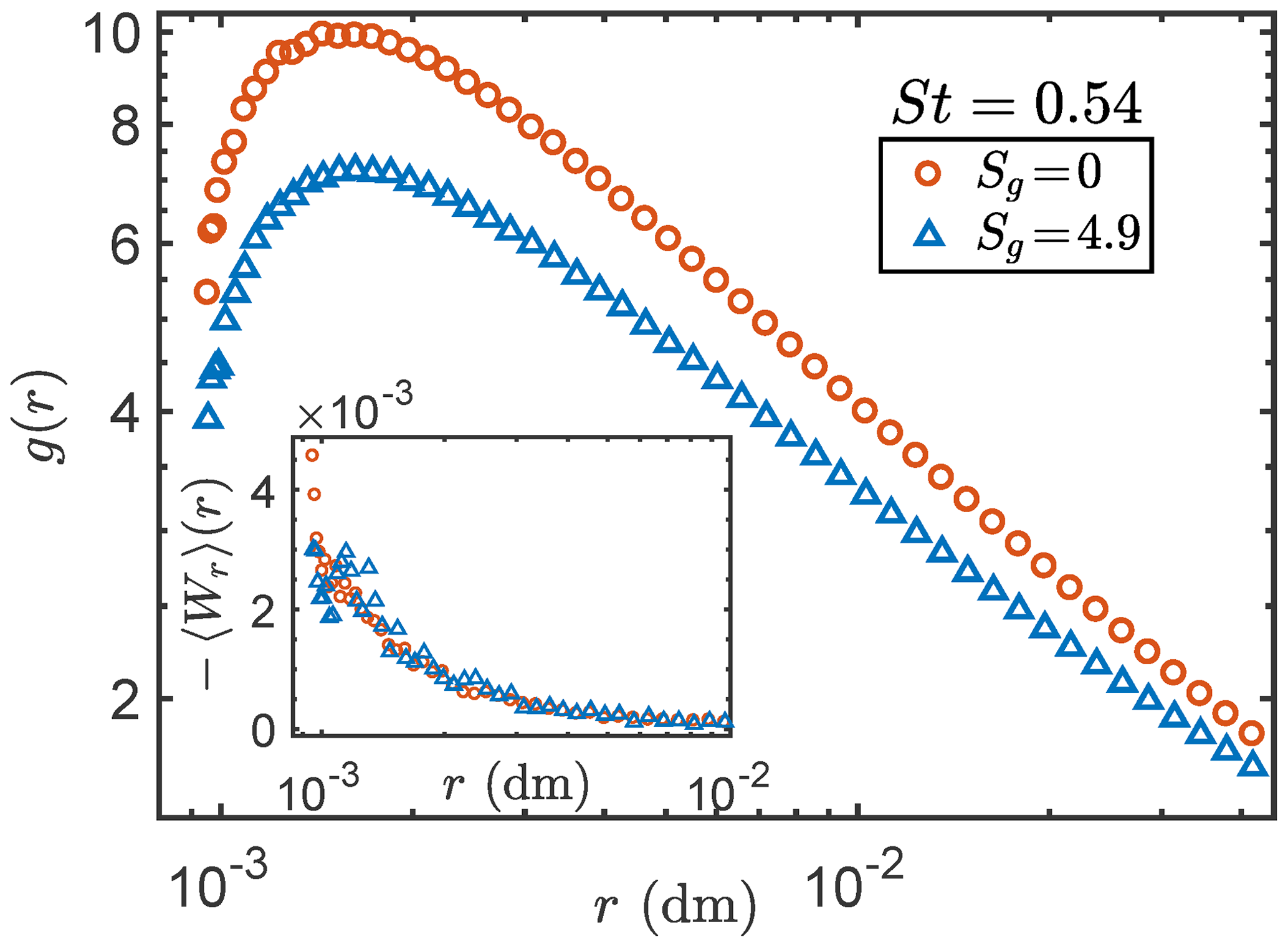
Figure 3 RDFs of particles (St=0.54) subject to action of turbulence and collision–coagulation with and without gravity. Circles: S_g=0 (zero gravity); triangles: S_g=4.9 (nonzero gravity). The latter shows a reduced slope in the power-law regime, while the shape of the two curves is largely similar in the collision regime (r∼d). Inset: MRVs of the same cases as in the main figure. Gravity weakens the MRV of the particles.

As mentioned, the fundamental focus of our work precludes the DNS and theory from considering a number of complexities relevant to some applications. As a result, this limits the direct quantitative applicability of our results to some realistic problems (e.g., in clouds). Besides gravity, another neglected factor is the hydrodynamic inter-particle force (HDI). Recent works, e.g., Yavuz et al. (2018); Bragg et al. (2022) found that the HDI also has a strong impact on RDF for r∼d. For monodisperse particles with small to moderate St, the HDI is expected to be more important than gravity. While we expect that the HDI should not alter the qualitative trend that g(r) should fall towards a small value at r→d (the same applies to the observed trend of MRV), it is likely that the HDI and collision would affect RDF and MRV in a coupled manner.

Also neglected is the influence of temperature, humidity and the vapor–liquid phase transition, which are important in the atmospheric clouds. These factors have a substantial impact on the polydispersity of small droplets (see, e.g., Kumar et al., 2012, 2014). However, for monodisperse statistics considered here, they are likely to play a minor role (they will be more important when future works consider the full polydisperse problem).

One limitation of the theory stems from the assumption of St≪1 and its corollary that particle velocity statistics in this regime are St-independent (Chun et al., 2005), which limits the theory's applicability to real systems. This implies that MRV should be St-independent in this regime. Our DNS results (spanning 2 orders of magnitude in St) shown in Fig. 2 give some support to the latter. However, unlike the theoretical prediction for MRV of case St=0.054 (Fig. 2), we have found that the prediction for St=0.11 is discernibly below the DNS result (figure in the Supplement). This could be due to the finite St effect not captured by the theory or could be for other reasons (details in the Supplement). Hence, a finite St extension of the theory is desirable to improve its applicability to real systems.

5 Conclusions

To conclude, we observed that collision strongly affects the RDF and MRV and imposes strong coupling between them⁶. This challenges the efficacy of a “separation paradigm” and suggests that results from any studies that preclude particle collision have limited relevance for predicting collision statistics. We have presented a theory for particle collision–coagulation in turbulence (based on a Fokker–Planck framework) that explains the above observations and verified its accuracy by showing that 〈W_r〉 could be accurately predicted using a sufficiently accurate RDF. The theory accounts for the full collision–coagulation rate, which includes contributions from mean field and fluctuations, and as such, our work complements and completes earlier mean-field theories (Saffman and Turner, 1956; Sundaram and Collins, 1997). We showed that a simple model of particle approach angles could capture the main features of 〈W_r〉 and used it to derive a general solution for RDF from the differential version of the theory. We uncovered a possible paradox regarding the past empirical successes of the differential drift-diffusion equation (see Sect. 4.4). Further shape-preserving reduction of the RDF and MRV was observed when the gravitational settling parameter (S_g) is of order O(1). Our findings provide new perspectives of particle collision and its relation with clustering and relative motion, which have implications for atmospheric clouds or generally for systems involving colliding particles in unsteady flows.