Quantifying albedo susceptibility biases in shallow clouds

The evaluation of radiative forcing associated with aerosol–cloud interactions remains a significant source of uncertainty in future climate projections. The problem is confounded by the fact that aerosol particles influence clouds locally and that averaging to larger spatial and/or temporal scales carries biases that depend on the heterogeneity and spatial correlation of the interacting fields and the nonlinearity of the responses. Mimicking commonly applied satellite data analyses for calculation of albedo susceptibility S_o, we quantify S_o aggregation biases using an ensemble of 127 large eddy simulations of marine stratocumulus. We explore the cloud field properties that control this spatial aggregation bias and quantify the bias for a large range of shallow stratocumulus cloud conditions manifesting a variety of morphologies and ranges of cloud fractions. We show that S_o spatial aggregation biases can be on the order of hundreds of percent, depending on the methodology. Key uncertainties emanate from the typically applied adiabatic drop concentration N_d retrieval, the correlation between aerosol and cloud fields, and the extent to which averaging reduces the variance in cloud albedo A_c and N_d. S_o biases are more often positive than negative and are highly correlated with biases in the liquid water path adjustment. Temporal aggregation biases are shown to offset spatial aggregation biases. Both spatial and temporal biases have significant implications for observationally based assessments of aerosol indirect effects and our inferences of underlying aerosol–cloud–radiation effects.

1 Introduction

Shallow liquid clouds are a poorly quantified component of the climate system and one of the greatest sources of uncertainty for climate projections (e.g., Bony and Dufresne, 2005; Bony et al., 2017). The problem is multifaceted and encompasses fundamental understanding of how these clouds are affected by the thermodynamic structure of the atmosphere, how they might change in a warmer world, how they are influenced by the atmospheric aerosol, and how all of these components are represented in climate models. The difficulty in quantifying the radiative effects of shallow clouds emanates, to a large extent, from the large range of spatiotemporal scales involved: aerosol–cloud interaction processes need to be understood and resolved at the scale of centimeters (e.g., Hoffmann et al., 2019), while cloud fields and their organization are driven by larger-scale circulations at scales of hundreds to thousands of kilometers (e.g., Norris and Klein, 2000). Importantly, aerosol–cloud interactions acting at scales on the order of 100 m need to be resolved, (a) because they can lead to fundamental changes in the radiative state of a cloud system by changing the cloud albedo, cloud fraction, and spatial distribution of condensate (e.g., Sharon et al., 2006; Stevens et al., 2005; Wang and Feingold, 2009) and (b) because nonlinearities in aerosol–cloud–radiation interactions mean that the methodology of averaging small-scale properties to larger scales might generate biases in the radiative response.

This paper focuses on the ramifications of small-scale processes for cloud albedo susceptibility and cloud liquid water path adjustments (changes in liquid water path in response to changes in aerosol concentration) within the context of how they are treated in satellite-based analyses. Two key aspects are addressed: the first relates to spatial averaging from the level of the satellite pixel (order 1 km) to commonly used aggregation scales on the order of tens to hundreds of kilometers, and the second relates to temporal aggregation from the individual scene snapshot up to a timeframe on the order of months. Large-scale analyses often aggregate data both spatially and temporally into data sets that might cover, e.g., $\mathrm{4}{}^{\circ }\times \mathrm{4}{}^{\circ }$ and 5 years (Chen et al., 2014), or a range of scales from kilometers to tens of kilometers for cloud microphysics, liquid water path, and radiation, $\mathrm{1}{}^{\circ }\times \mathrm{1}{}^{\circ }$ for aerosol, and 3-month seasonal responses (Lebsock et al., 2008). While it is impractical not to aggregate to some degree, e.g., to smooth noisy retrievals or extract signals from a noisy background, the implications for quantifying aerosol–cloud interactions are still not well understood.

In the following, we will use the terms “aggregation” and “averaging” synonymously; “aggregation” tends to be used when speaking more broadly about including data from a larger range of spatial and temporal scales, whereas “averaging” is used in more of a mathematical sense.

We quantify aerosol–cloud interactions using the albedo susceptibility metric (Platnick and Twomey, 1994) defined here as

$$\begin{array}{}\text{(1)}& S_{\mathrm{o}}={\displaystyle \frac{d\ln A_{\mathrm{c}}}{d\ln N_{\mathrm{d}}}}={\displaystyle \frac{\left(\mathrm{1}-A_{\mathrm{c}}\right)}{\mathrm{3}}}\left[\mathrm{1}+{\displaystyle \frac{\mathrm{5}}{\mathrm{2}}}{\displaystyle \frac{d\ln \mathcal{L}}{d\ln N_{\mathrm{d}}}}\right],\end{array}$$

where A_c is the cloud albedo, N_d is the drop concentration, and ℒ is the liquid water path. The expression comprises the cloud brightening or Twomey component $(\mathrm{1}-A_{\mathrm{c}})/\mathrm{3}$ and the adjustment term ${\mathcal{L}}_{\mathrm{o}}=d\ln \mathcal{L}/d\ln N_{\mathrm{d}}$ and assumes no changes in drop distribution width (e.g., Feingold and Siebert, 2009). The factor of $\mathrm{5}/\mathrm{2}$ suggests a potentially strong but uncertain contribution from ℒ adjustments; even the sign of this term varies from positive for precipitating clouds to negative for non-precipitating clouds (Christensen and Stephens, 2011; Glassmeier et al., 2021).

Using satellite-based observation systems, e.g., the MODerate Imaging Spectroradiometer (MODIS; Salomonson et al., 1998), one can derive a drop concentration N_d,a, based on adiabatic assumptions, from retrieved visible cloud optical depth τ and cloud-top drop effective radius r_e:

$$\begin{array}{}\text{(2)}& N_{\mathrm{d},\mathrm{a}}={\displaystyle \frac{\sqrt{\mathrm{5}}}{\mathrm{2}\mathit{\pi }k}}{\left({\displaystyle \frac{f_{\mathrm{ad}}{c}_{\mathrm{w}}(T,P)\mathit{\tau }}{Q_{\mathrm{ext}}{\mathit{\rho }}_{\mathrm{w}}{r}_{\mathrm{e}}^{\mathrm{5}}}}\right)}^{\mathrm{1}/\mathrm{2}},\end{array}$$

where c_w(T,P) is related to the condensation rate and is a known function of cloud-base temperature T and pressure P, f_ad is the adiabatic fraction (assumed in this paper to be 0.8), Q_ext is the extinction coefficient (≈2 in the visible part of the spectrum), ρ_w is the density of liquid water, and k is a factor that is inversely proportional to the width of the drop size distribution (assumed to be 0.8). When f_ad=1, N_d,a is the adiabatic drop concentration.

Liquid water path ℒ is derived from MODIS data as

$$\begin{array}{}\text{(3)}& \mathcal{L}={\displaystyle \frac{\mathrm{5}}{\mathrm{9}}}{f}_{\mathrm{ad}}{r}_{\mathrm{e}}\mathit{\tau }.\end{array}$$

Further details of these derivations can be found in Brenguier et al. (2000) and Grosvenor et al. (2018). A_c can be derived from τ using a simple two-stream approximation for a plane-parallel cloud (Bohren, 1987):

$$\begin{array}{}\text{(4)}& A_{\mathrm{c}}={\displaystyle \frac{\mathit{\tau }}{\mathit{\gamma }+\mathit{\tau }}},\end{array}$$

where γ depends on the degree of forward scattering. Equation (4) also assumes an overhead sun, no absorption, and a dark underlying surface. We do not consider three-dimensional radiative transfer.

As an example of how averaging of data can affect the quantification of derived variables, we note that Eq. (4) is a concave function, which, following Jensen's inequality, means that for an inhomogeneous cloud field, $f\left(\stackrel{\mathrm{‾}}{\mathit{\tau }}\right)>\stackrel{\mathrm{‾}}{f\left(\mathit{\tau }\right)}$. Thus, calculating τ based on large length-scale-averaged cloud properties and then calculating $A_{\mathrm{c}}=f\left(\stackrel{\mathrm{‾}}{\mathit{\tau }}\right)$ using Eq. (4) will generate a high bias in A_c that is inherently a function of the inhomogeneity of the cloud field. Because this well-known albedo bias (e.g., Cahalan et al., 1994; Oreopoulos and Davies, 1998) is not the topic of this paper, we will assume in all calculations that A_c is measured directly by an instrument like Clouds and the Earth's Radiant Energy System (CERES) at the desired measurement length scale and therefore does not suffer from an averaging bias. Instead, we explore similar biases that affect quantification of S_o. For example, Eq. (2) is a highly nonlinear function of τ and r_e so that whether one elects to calculate N_d,a before or after averaging of component variables τ and r_e will potentially have a strong effect on S_o.

McComiskey and Feingold (2012) analyzed large eddy simulation (LES) output of three cloud fields characterized by different degrees of inhomogeneity and showed that an aerosol–cloud interaction metric, $d\ln \mathit{\tau }/d\ln N_{\mathrm{d}}$, increased as a result of averaging – more so for heterogeneous fields than for homogeneous fields. To put the topic on firmer footing, we first establish a theoretical framework for assessing the biases. We then use a large number of LESs (127) as proxy data, which we use to simulate satellite retrievals. We apply typical methodologies used in satellite retrievals, as well as variants, to assess the provenance of the S_o bias. Both spatial and temporal aggregation scales are considered, with a focus on the former. Because of the limited domain size available to LES, we concern ourselves with the effects of spatial averaging from scales on the order of 1 to 10 km. The multiple snapshots of different scenarios available from the LES output provide the basis for temporal aggregation. We note that Grandey and Stier (2010) also looked at the effect of aggregation scale on quantification of aerosol indirect effects (the radiative forcing of aerosol–cloud interactions). Their analysis addressed much larger scales (1, 4, and 60^∘) in climate models. Here we focus on a model framework that explicitly resolves aerosol–cloud interactions at the cloud scale.

2 Theory

2.1 Spatial aggregation of variables derived from nonlinear functions

The two fundamental geophysical variables associated with aerosol–cloud interactions are N (a generic concentration or drop or aerosol number concentration, which are well correlated) and ℒ. In the case of homogeneous aerosol and cloud fields, averaging of data to different scales has no effect on derived quantities such as N_d, ℒ, A_c, and S_o, and the order of calculation of these fields is of no consequence. In reality, however, cloud fields exhibit different degrees of inhomogeneity: condensation of cloud water responds to local updrafts and, to some extent, availability of cloud condensation nuclei. Drop concentration depends on aerosol concentration – typically a less variable field than cloud water – as well as local supersaturation driven by updrafts. Under these conditions, the quantification of aerosol–cloud interaction metrics like S_o and the influence of averaging could be far more important.

The theoretical framework for addressing this question is well known from similar examples in the atmospheric sciences, notably biases in rain formation processes that result from large-scale averaging of the cloud water and drop concentration terms in expressions for autoconversion and accretion (e.g., Lebsock et al., 2013; Zhang et al., 2019). In the interest of completeness, we repeat the key equations here. Assuming a lognormal probability distribution function (PDF) of quantity x,

$$\begin{array}{}\text{(5)}& P\left(x\right)={\displaystyle \frac{\mathrm{1}}{\sqrt{\mathrm{2}\mathit{\pi }}x\ln {\mathit{\sigma }}_{\mathrm{g},x}}}\exp \left[-\left(x-x_{\mathrm{g}}\right)/\left(\mathrm{2}{\ln }^{\mathrm{2}}{\mathit{\sigma }}_{g,x}\right)\right],\end{array}$$

where the lognormal parameters are geometric mean (or median) x_g and geometric standard deviation σ_g,x. Quantity x represents A_c or ℒ and N. Using well-known integral properties of the lognormal function (e.g., Feingold and Levin, 1986), it is easy to show that the bias in a moment $x^{{\mathit{\beta }}_x}$ associated with averaging can be written as

$$\begin{array}{}\text{(6)}& B_x={\displaystyle \frac{\stackrel{\mathrm{‾}}{x^{{\mathit{\beta }}_x}}}{{\stackrel{\mathrm{‾}}{x}}^{{\mathit{\beta }}_x}}}={\left(D_x^{\mathrm{2}}+\mathrm{1}\right)}^{\frac{{\mathit{\beta }}_x^{\mathrm{2}}-{\mathit{\beta }}_x}{\mathrm{2}}},\end{array}$$

with the relative dispersion D_x, the ratio of the standard deviation to the mean, defined as

$$\begin{array}{}\text{(7)}& D_x={\left(\stackrel{\mathrm{‾}}{(x-\stackrel{\mathrm{‾}}{x}{)}^{\mathrm{2}}}\right)}^{\mathrm{1}/\mathrm{2}}/\stackrel{\mathrm{‾}}{x}.\end{array}$$

If the two interacting fields, e.g., ℒ and N, are assumed to follow a bivariate lognormal distribution, the bias associated with the covariance between ℒ and N is

$$\begin{array}{}\text{(8)}& B_{\mathrm{cov}}=\exp \left(r\right(\mathcal{L},N)\cdot {\mathit{\beta }}_{\mathcal{L}}\cdot {\mathit{\beta }}_N\cdot {\mathit{\sigma }}_{\mathrm{g},\mathcal{L}}\cdot {\mathit{\sigma }}_{\mathrm{g},N}),\end{array}$$

where r(ℒ,N) is the spatial correlation between ℒ and N. (Note that we elect to present the theory in terms of ℒ and N rather than A_c and N because A_c includes compounded dependence on N via τ. Since ℒ and A_c are highly correlated, this choice does not affect the general framework for discussion.)

The overall bias associated with averaging for two covarying fields is then given by

$$\begin{array}{}\text{(9)}& B=B_{\mathcal{L}}\cdot B_N\cdot B_{\mathrm{cov}}.\end{array}$$

The equations allow theoretical calculation of the S_o biases associated with two covarying fields ℒ and N, each characterized by its own heterogeneity D_ℒ and D_N, respectively.

To apply this analysis to biases in S_o associated with interacting ℒ and N fields, we make a number of assumptions. In the absence of an analytical form for the ℒ adjustment, we assume it is negligible. We also assume that A_c depends linearly on τ, which holds over a large range of τ. S_o is then approximated as being proportional to 1−τ (Eq. 1). Note that because the percent bias in 1−τ is equivalent to the percent bias in τ, we can apply

$$\begin{array}{}\text{(10)}& \mathit{\tau }=c{\mathcal{L}}^{\mathrm{5}/\mathrm{6}}{N}^{\mathrm{1}/\mathrm{3}}\end{array}$$

(e.g., Brenguier et al., 2000), where c is a constant that does not require specification for the purpose of the current analysis. Then, with ${\mathit{\beta }}_{\mathcal{L}}=\mathrm{5}/\mathrm{6}$ and ${\mathit{\beta }}_N=\mathrm{1}/\mathrm{3}$, Eq. (9) can be calculated for given values of D_ℒ, D_N, and r(ℒ, N). These are shown in Fig. 1 in D_ℒ; D_N space for three values of r(ℒ, N). We note that large positive and negative biases can result from averaging; for negative r(ℒ, N), biases are positive and on the order of 20 %–60 %, whereas for positive values of r(ℒ,N), biases are negative and on the order of −20 % to −70 %. When correlation between the fields is zero, biases are 10 %–20 %. The central role of r(ℒ, N) is further illuminated by plotting the bias in S_o as a function of r(ℒ, N) for specified D_ℒ and D_N combinations (Fig. 2).

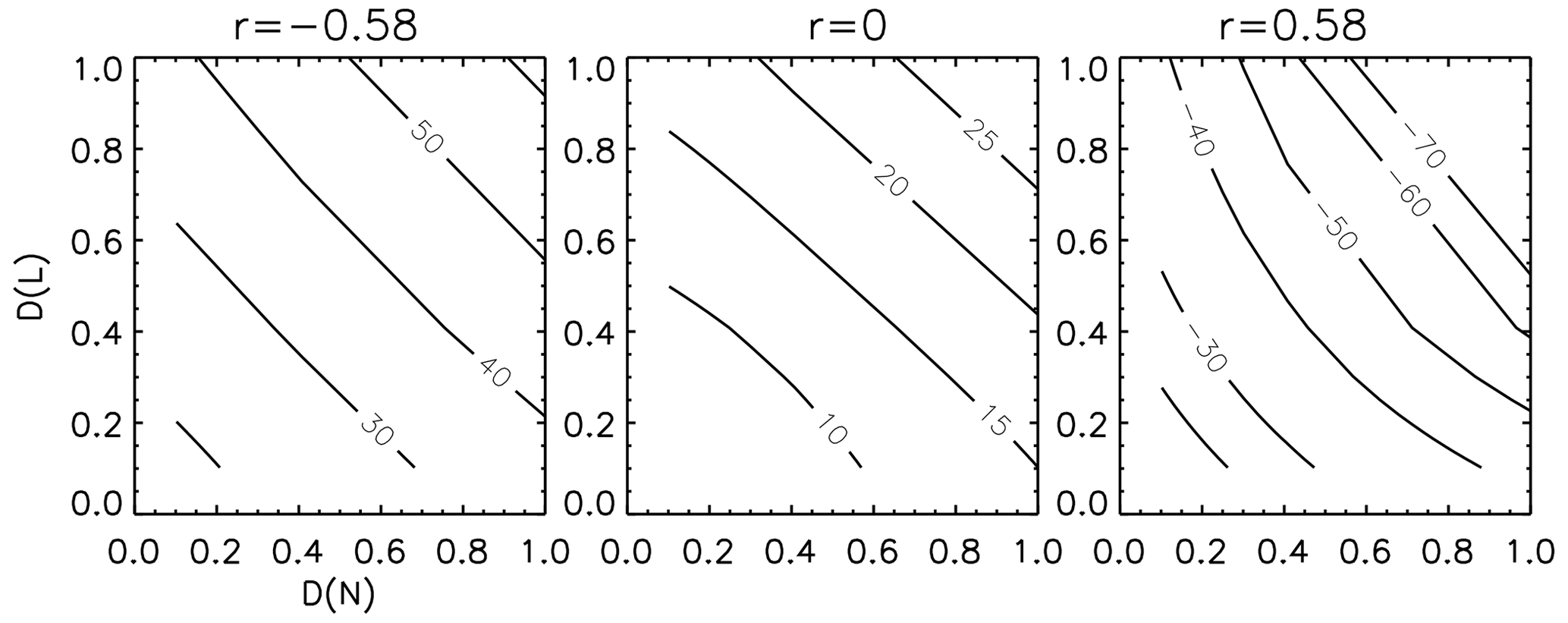
Figure 1 Theoretical calculations of the albedo susceptibility bias (%) for a range of relative dispersions in ℒ and N (D(ℒ) and D(N), respectively) for three different correlations (r) between ℒ and N. Note the values of large positive and negative biases.

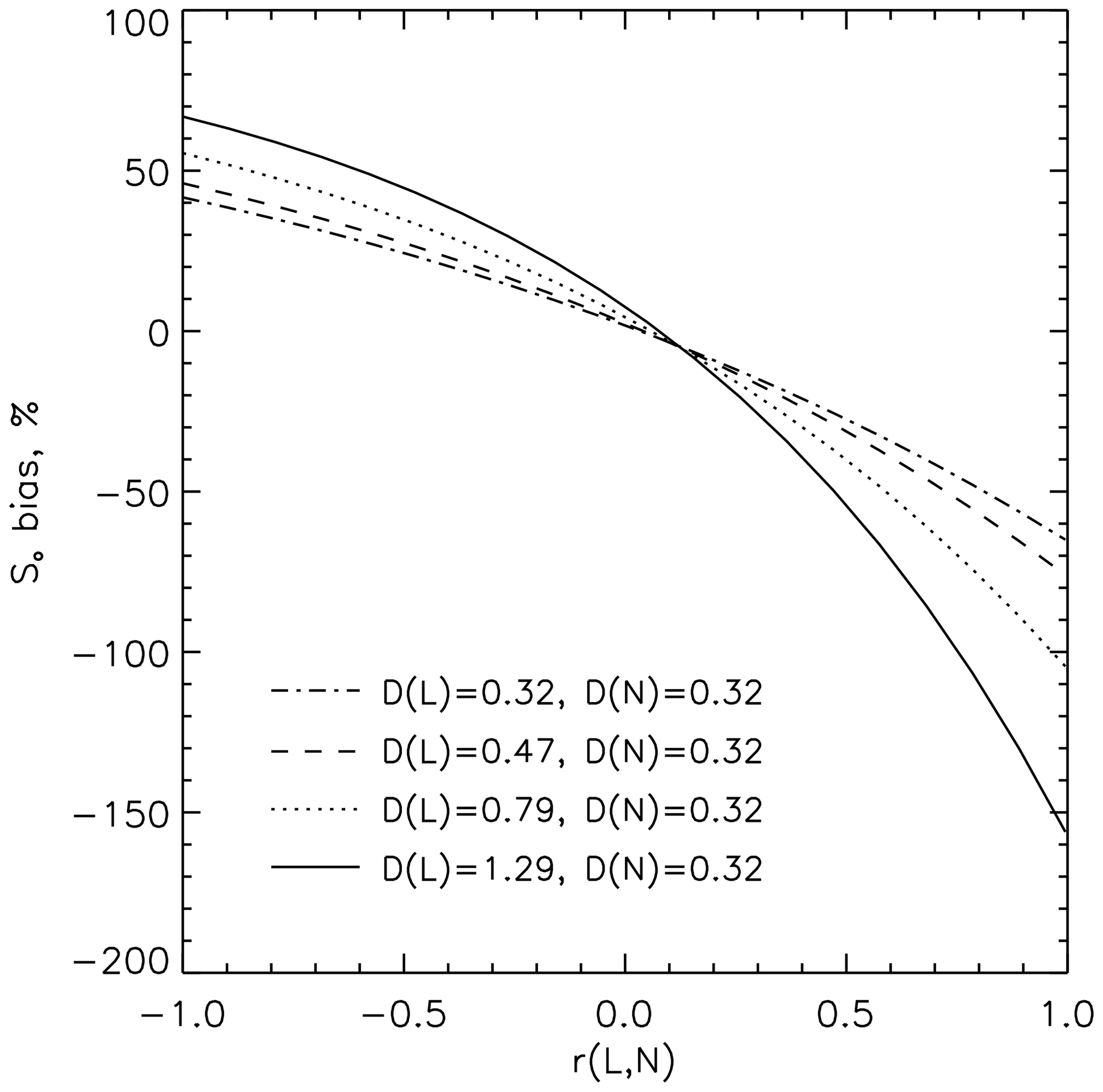
Figure 2 As in Fig. 4 but for the S_o bias as a function of the spatial correlation between ℒ and N for a range of relative dispersions in ℒ (D(ℒ)) and fixed D(N). Of note is that for the conditions shown the biases are large and range from about −150 % (positive r, large D(ℒ)) to +70 % (negative r, large D(ℒ)).

Note that the assumption of a bivariate lognormal distribution is common when dealing with geophysical fields. Another cautionary note is that, given the various assumptions applied to generate the results in Figs. 1 and 2, they should be considered illustrative; i.e., they are primarily intended to highlight key variables that control aggregation bias. When we embark on our analysis of LES output, we will assume that τ and r_e are known exactly, and quantitative comparison with Figs. 1 and 2 should be avoided.

2.2 Effects of spatial and temporal averaging on variance, and correlation between fields

The second framework for assessment of biases derives from the basic definition of the linear regression fit:

$$\begin{array}{}\text{(11)}& \widehat{b}=r_{x,y}{\displaystyle \frac{{\mathit{\sigma }}_y}{{\mathit{\sigma }}_x}},\end{array}$$

where $\widehat{b}$ is the regression slope and σ_x is the standard deviation of field x. In our case, x is aerosol or drop concentration (we will use N_d) and y is the cloud variable (A_c or ℒ). As shown by McComiskey and Feingold (2012), averaging increases r(x,y) but decreases σ_x and σ_y to varying degrees. Of interest is therefore the extent to which averaging changes r(x,y) and the ratio ${\mathit{\sigma }}_y/{\mathit{\sigma }}_x$.

3 Large eddy simulation as a data source

We calculate S_o biases using output from 127 large eddy simulations of marine stratocumulus under a range of conditions from fairly homogeneous overcast to broken open-cellular structures.

Simulations are generated by the System for Atmospheric Modeling (SAM; Khairoutdinov and Randall, 2003). Input conditions are derived from ERA-5 reanalysis in the stratocumulus regime off the coast of California. The model setup is similar to Feingold et al. (2016) and Glassmeier et al. (2021), with initial meteorological and aerosol conditions sampled using the Latin hypercube method. Simulations are nocturnal and of 12 h duration. The first 5 h of output from each simulation is discarded to avoid cloud scenes that are not fully developed. The domain size is 48 km × 48 km × 2.5 km with a 500 m damping layer below the model top at 2.5 km. The profile is extended up to 35 km (5 hPa) for radiation calculations. Grid spacings are $\mathrm{d}x=\mathrm{d}y=\mathrm{200}$ m and dz=10 m. A two-moment bulk microphysical method that calculates all warm cloud processes (including supersaturation and activation) is applied (Feingold et al., 1998). The simulations differ from Glassmeier et al. (2021) in one key respect, namely, that surface fluxes are calculated interactively. Resultant cloud fields exhibit varying degrees of heterogeneity, including closed-, open-, and transitions from closed- to open-cellular convection.

The LES output provides microphysical fields of drop number concentration and liquid water content as three-dimensional prognostic variables under the assumption of a bimodal lognormal distribution of cloud drops and raindrops with fixed distribution width (σ_g=1.2 for both). However, to mimic satellite retrievals, we work with the derived model variables τ and cloud-top r_e to calculate N_d and ℒ based on Eqs. (2) and (3). Both cloud water and rainwater contribute to τ and r_e. Cloud top is calculated based on a liquid water mixing ratio threshold (0.01 g kg⁻¹). Because these clouds are strongly capped, the first grid point exceeding this value (when working from above and downward towards the cloud top) almost always exceeds the threshold significantly, providing a maximum or near-maximum r_e in each model column. A_c is calculated based on the modeled value of τ (Eq. 4), is then averaged, and therefore does not suffer from averaging bias. S_o is calculated directly for each scene based on the definition ($S_{\mathrm{o}}=d\ln A_{\mathrm{c}}/d\ln N_{\mathrm{d}}$) using least squares regression to the natural logarithms of A_c and N_d.

3.1 Spatial aggregation

3.1.1 Level-2 analysis

The standard averaging method follows the MODIS level-2 (L2) methodology in the sense that calculations are performed at high resolution prior to averaging. In the current work, Eqs. (2) and (3) are calculated based on the native 200 m model mesh (n=1) and then averaged to n×n tiles. Results will be shown for n=30 vs. n=4, i.e., 6 km × 6 km boxes vs. 800 m × 800 m boxes. These choices result from a desire for a reasonable number of regression points (n=30) and for some small amount of smoothing (n=4) to reduce the noise in N_d retrievals (Eq. 2). The choice of n=4 also brings us close to the typical 1 km length scale used for analysis of L2 MODIS data. (We did not use n=5, i.e., 1 km, because the number of points in the domain is even, and our desire is to maximize our coverage and simplify analysis.) Note that L2 methodology removes the biases associated with nonlinear functions applied to averaged data discussed in Sect. 2.1 (Jensen's inequality) since N_d is calculated using Eq. (2) at the 200 m level and then averaged up. The same is true for A_c, which as previously noted is calculated based on Eq. (4).

Biases are defined as

$$\begin{array}{}\text{(12)}& (\stackrel{\mathrm{‾}}{X}-X)/X,\end{array}$$

where X represents S_o calculated at n=4 and $\stackrel{\mathrm{‾}}{X}$ represents S_o at n=30. Correlations r(ℒ,N_d) refer to calculations for n=4 unless otherwise stated. N_d in the L2 analysis represents cloudy-column averaged drop concentration, i.e., $N_{\mathrm{d}}=N_{\mathrm{d},\mathrm{a}}$ based on Eq. (2).

The N_d retrieval (Eq. 2) is very sensitive to thin clouds, particularly when r_e but also τ are small. As is common in MODIS data analyses, calculations are only applied to thicker clouds, in our case to r_e>3 µm and τ>3.

3.1.2 Variants

Two variants of the calculations will be presented.

1. Mimic MODIS level-3 (L3) analysis. Here satellite-based retrievals are based on aggregated data. In other words, Eqs. (2) and (3) for N_d and ℒ, respectively, are applied to data averaged to n=4 and n=30. By doing so the averaging biases associated with Jensen's inequality are introduced. The biases are expected to derive from a mix of influences: low for N_d (a convex function in r_e dominates a concave function in τ; Eq. 2) and negligible for ℒ (Eq. 3). The effect of smoothing associated with level-3 aggregation is thus likely to be highly dependent on cloud field heterogeneity.

2. Mimic MODIS L2 analysis but eliminate uncertainties in the (sub)adiabatic retrieval of N_d by assuming a “perfect” N_d, which is taken directly from the LES. Because the LES N_d is a three-dimensional variable, we use in-cloud, column average values. This methodology will be referred to as L2_N. Note that ℒ is still calculated as per Eq. (3). The goal here is to understand the extent to which the retrieval of N_d drives the regression biases.

3.2 Temporal aggregation

To address temporal aggregation, we consider the same individual LES snapshots described above but calculate S_o in two ways: (i) S_o regression fits to individual cloud scenes are simply averaged up over all cloud scenes, and (ii) LES output is temporally aggregated to a large data set from which S_o is calculated via regression. The first approach preserves the individual cloud scene susceptibilities, while the second aggregates many different cloud fields before performing the regression. The biases are calculated based on Eq. (12), with the overbar indicating the second approach (ii). The methodology is followed (separately) for both n=4 and n=30 spatial averaging and for L2, L3, and L2_N.

4 Results

4.1 Spatial aggregation

4.1.1 Effect of spatial aggregation on S_o and correlation

Figure 3 presents results for the three approaches (L2, L3, and L2_N). We start with the figures showing ${\stackrel{\mathrm{‾}}{S}}_{\mathrm{o}}$ vs. S_o to avoid ambiguity in the sign of the bias associated with Eq. (12). (According to Eq. 12, conditions under which ${\stackrel{\mathrm{‾}}{S}}_{\mathrm{o}}$ is more negative than S_o also manifest as positive biases.) The solid line is the 1:1 line.

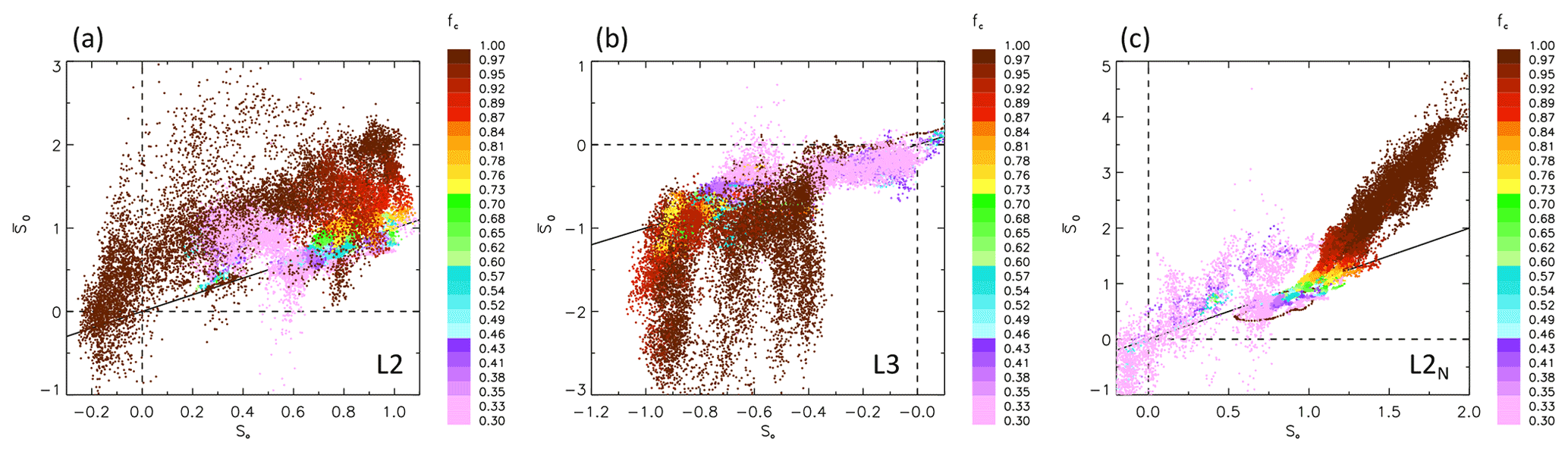
Figure 3 S_o aggregated to a 6 km scale (${\stackrel{\mathrm{‾}}{S}}_{\mathrm{o}}$) vs. S_o aggregated to an 800 m scale (S_o) for the (a) L2, (b) L3, and (c) L2_N methodologies as described in the text. Solid line is the 1:1 line. Dashed lines are drawn at ordinate and abscissa values of zero. Note the general overestimate in S_o with increasing aggregation scale in (a) and (c) and the change in sign in S_o associated with L3 aggregation in (b). Of note is that high-cloud-fraction/low-heterogeneity conditions are often associated with high biases.

Points are colored by cloud fraction f_c (defined at the native 200 m grid spacing) since it also serves as a good proxy for cloud field heterogeneity. (The correlation between f_c and D(ℒ) is 0.86.) For L2, we note that both ${\stackrel{\mathrm{‾}}{S}}_{\mathrm{o}}$ and S_o are almost always positive and that low-f_c states do not suffer from worse biases than high-f_c states. By contrast, high f_c is often associated with the largest biases. The reasons for this will become apparent in the subsequent analysis.

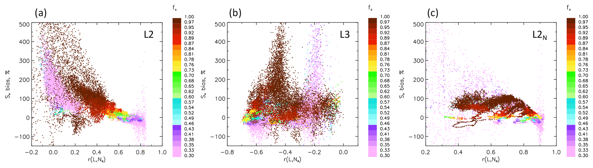
Figure 4 S_o bias in percent as defined in Eq. (12) as a function of the correlation between liquid water path and drop concentration r(ℒ, N_d) with points colored by cloud fraction f_c for the (a) L2, (b) L3, and (c) L2_N methodologies. In (a) and (c) the S_o bias tends to increase with decreasing r(ℒ, N_d) and increasing cloud fraction f_c, with noted exceptions. Use of the true N_d in (c) restricts the S_o bias to about 100 %.

Responses for the L3 analysis are distinctly different in a number of ways: first, both ${\stackrel{\mathrm{‾}}{S}}_{\mathrm{o}}$ and S_o are almost always negative, and low-f_c cloud scenes often have lower biases than high-f_c scenes. This is because L3 averaging has a stronger smoothing effect on broken cloud fields and therefore somewhat unexpectedly reduces the averaging bias for broken cloud fields compared to solid cloud fields. Nevertheless, the non-physical shift in the sign of S_o associated with the L3 methodology should act as a cautionary note. We present an explanation for the reversal of sign in Appendix A.

L2_N analysis yields strongly positive S_o and a clearer dependence of the bias on f_c. For broken cloud scenes S_o is sometimes negative, but biases tend to be scattered and relatively small. These low f_c≈0.3 states are dominated by cumulus cells with stronger updrafts that result in coherent N_d. Since S_o and ${\stackrel{\mathrm{‾}}{S}}_{\mathrm{o}}$ are only calculated in cloudy regions (above the r_e and τ thresholds), this coherence in N_d results in a small bias. Thus the reasons for small susceptibility bias at low f_c differ for L3 and L2_N. With increasing f_c, biases tighten around the 1:1 line but start to deviate for f_c>0.85 and exhibit increasingly large values.

To quantify the biases, these same analyses are shown as percent biases in S_o (Eq. 12) as a function of the correlation between ℒ and N_d (r(ℒ, N_d); Fig. 4), the calculations of which are consistent with the derivation of variables averaged to n=4; e.g., L2 and L3 calculations apply r(ℒ, N_d) based on Eqs. (2) and (3), and L2_N calculates r(ℒ, N_d) using the true N_d and Eq. (3).

L2 biases are almost always positive and can reach values of many hundreds of percent (Fig. 4). As expected from Sect. 2.1, r(ℒ, N_d) has a strong influence on the S_o bias, particularly for L2, with the bias increasing noticeably with decreasing r(ℒ, N_d) in a manner qualitatively similar to Fig. 2. The high values and high variability in the bias as one approaches r(ℒ, N_d)≈0 are to some extent a consequence of an uncertain regression fit when the correlation between the ℒ (or the closely related A_c) and N_d fields is poor.

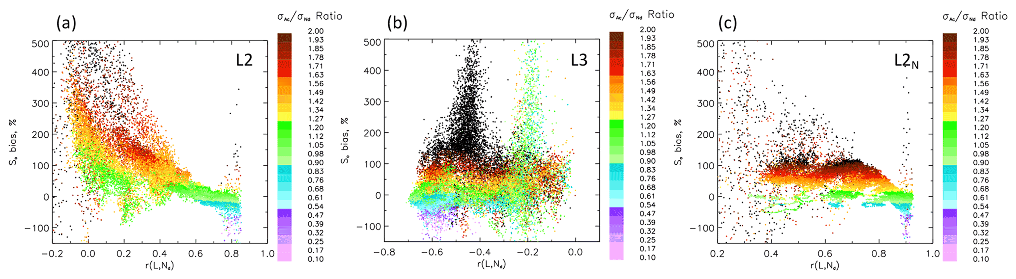
Figure 5 As in Fig. 4 but with points colored by the ratio of ${\mathit{\sigma }}_{A_{\mathrm{c}}}/{\mathit{\sigma }}_{N_{\mathrm{d}}}$ at 6 km to ${\mathit{\sigma }}_{A_{\mathrm{c}}}/{\mathit{\sigma }}_{N_{\mathrm{d}}}$ at 800 m (the σ ratio). Note the clear dependence of the S_o bias on the σ ratio and that the bias ∼0 when the σ ratio ∼1 (green colors). Exceptions to the latter occur for L2 at low r(ℒ, N_d).

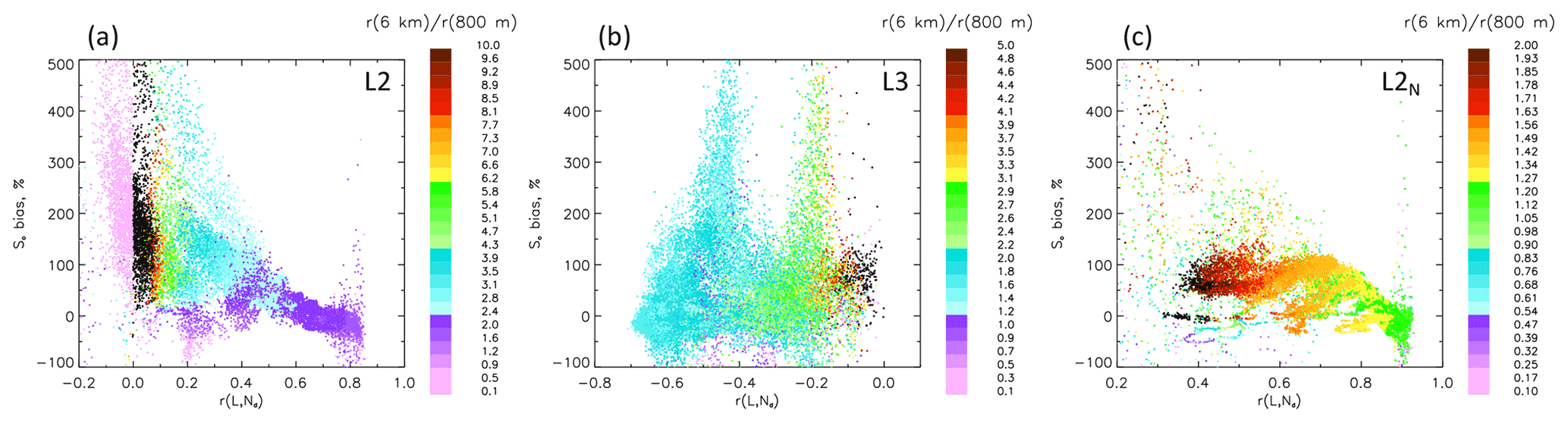
Figure 6 As in Fig. 4 but with points colored by the ratio of correlations r(ℒ, N_d) at 6 km to r(ℒ, N_d) at 800 m (the r ratio). Comparison with Fig. 5 shows approximately orthogonal dependence of the σ and r ratios on the S_o bias. In (a) and (b), calculation of the r ratio is mathematically unstable at r(ℒ, N_d)=0, as evidenced by saturating colors.

Of note is that the L3 analysis methodology (aggregate first and then derive) changes the sign of r(ℒ, N_d) to negative values, as it did the sign of S_o (Fig. 3). L3 biases are more widely dispersed and show no clear trend with r(ℒ, N_d) or f_c. L2_N biases tend to be capped at about 100 %, and values of r(ℒ, N_d) are noticeably more positive than those in L2. These results reinforce two points, (i) that L3 analysis generates non-physical results, negative S_o, and a change in the sign of r(ℒ, N_d), and (ii) that the use of the (sub)adiabatic assumption (Eq. 2) as a proxy for N_d incurs a significant increase in the S_o bias relative to L2_N, most noticeably at low r(ℒ, N_d), where Eq. (2) results in a significantly reduced (but for the most part positive) correlation.

4.1.2 Effect of spatial aggregation on regression

It is useful to turn to the underlying definitions of regression analysis (Sect. 2.2) to explore more deeply the influence of averaging on the S_o bias. According to Eq. (11), S_o biases are related to the ratio of $\widehat{b}$ (6 km) to $\widehat{b}$ (800 m):

$$\begin{array}{}\text{(13)}& \stackrel{\mathrm{‾}}{\widehat{b}}/\widehat{b}={\displaystyle \frac{{\stackrel{\mathrm{‾}}{r}}_{x,y}}{r_{x,y}}}\left({\displaystyle \frac{{\stackrel{\mathrm{‾}}{\mathit{\sigma }}}_y}{{\stackrel{\mathrm{‾}}{\mathit{\sigma }}}_x}}\right)/\left({\displaystyle \frac{{\mathit{\sigma }}_y}{{\mathit{\sigma }}_x}}\right),\end{array}$$

with $\stackrel{\mathrm{‾}}{\widehat{b}}$ denoting 6 km averaging and $\widehat{b}$ denoting 800 m averaging. We therefore consider (i) the ratio ${\stackrel{\mathrm{‾}}{\mathit{\sigma }}}_{A_{\mathrm{c}}}/{\stackrel{\mathrm{‾}}{\mathit{\sigma }}}_{N_{\mathrm{d}}}$ to ${\mathit{\sigma }}_{A_{\mathrm{c}}}/{\mathit{\sigma }}_{N_{\mathrm{d}}}$ (henceforth the “σ ratio”; Fig. 5) and (ii) the ratio $\stackrel{\mathrm{‾}}{r}(A_{\mathrm{c}},N_{\mathrm{d}})/r(A_{\mathrm{c}},N_{\mathrm{d}})$ (henceforth the “r ratio”; Fig. 6), which by Eq. (11) are both determinants of the bias. Note that, for the r ratio, we use r(A_c, N_d) to adhere more rigorously to the regression analysis definitions. The interpretation of these ratios is non-trivial. They express the extent to which ${\mathit{\sigma }}_{A_{\mathrm{c}}}/{\mathit{\sigma }}_{N_{\mathrm{d}}}$ and r(A_c, N_d) are modified by averaging. In the case of ${\mathit{\sigma }}_{A_{\mathrm{c}}}/{\mathit{\sigma }}_{N_{\mathrm{d}}}$ this amounts to interpreting a “ratio of ratios”. Later we will delve into this in more detail.

L2 results show a clear dependence of the S_o bias on the σ ratio and especially large biases when the σ ratio is high (Fig. 5a). These also happen to be points exhibiting high f_c (cf. Fig. 4a). Also apparent is that the separation of positive and negative biases is demarcated at a σ ratio of 1. The results suggest a strong correlation between the σ ratio and f_c. At high r(ℒ, N_d), the S_o bias increases systematically with increasing σ ratio (Fig. 5a), but with decreasing r(ℒ, N_d) the strong and orthogonal influence of the r ratio becomes more important (Fig. 6a). Clearly evident in Fig. 6a is the anticipated unstable calculation of the r ratio in the vicinity of r(ℒ, N_d)=0.

The L3 methodology exhibits an even clearer dependence of the S_o bias on the σ ratio, except for cloud fields with r(ℒ, $N_{\mathrm{d}})\approx -\mathrm{0.2}$ (Fig. 5b), where the high bias is clearly related to both the σ and r ratios (Fig. 6b). The aforementioned vertically oriented green-colored points have a σ ratio of about 1 and an r ratio of 2.5; i.e., the bias is driven by the r ratio.

For the L2_N methodology, here too the σ ratio (Fig. 5c) provides a clearer indication of the magnitude of the bias compared to either the r ratio (Fig. 6c) or f_c (Fig. 4).

Figure 7 Effects of aggregation on normalized reduction in σ(A_c) vs. normalized reduction in σ(N_d) to shed light on results in Fig. 5. Points are colored by f_c. (a–c) At high (low) f_c averaging tends to more significantly reduce (increase) σ(N_d) relative to σ(A_c). Notable exceptions occur in (c) for some low-f_c conditions. See text for further discussion.

Figure 8 As in Fig. 7 but with points colored by the r ratio. See text for discussion.

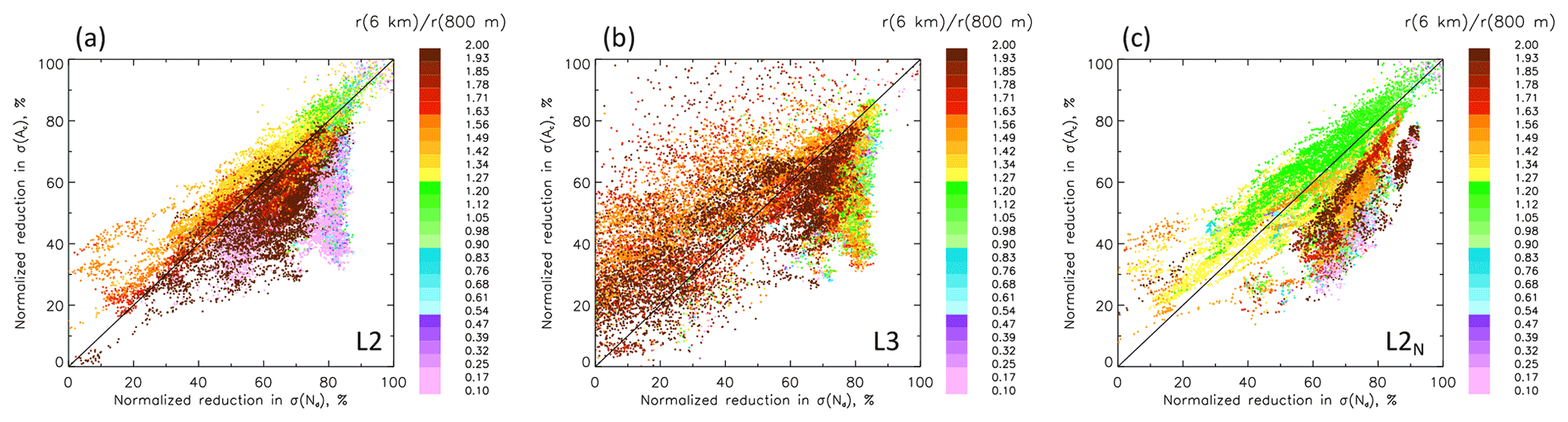
Based on Eq. (13), the influence of the σ and r ratios on S_o bias is expected. What is more revealing is the influence of averaging on the components of these ratios. To this end, Fig. 7 examines the effect of averaging on the reduction in ${\mathit{\sigma }}_{A_{\mathrm{c}}}$ and ${\mathit{\sigma }}_{N_{\mathrm{d}}}$. In other words, we ask to what extent averaging smoothens the A_c field relative to the smoothing in the N_d field. Accordingly, axes in Fig. 7 are calculated as normalized reductions in the variables.

L2 analysis shows that at low f_c the normalized reductions in σ(N_d) tend to be smaller than those in σ(A_c) but that the reverse tends to be true for f_c>0.75 (Fig. 7a); i.e., at high f_c, averaging smoothens the N_d field more than it smoothens the A_c field. We will show below that these high-f_c scenes, although inherently more homogeneous, often manifest significant inhomogeneity in N_d as a result of the N_d retrieval. (See further discussion in Sect. 4.1.4, Examples.)

The clear exception to the trend of averaging and smoothing N_d more than A_c with increasing f_c is the group of low-f_c points that exists in Fig. 4a at $r(\mathcal{L},N_{\mathrm{d}})<\mathrm{0.2}$. These anomalous points appear below the 1:1 line in Fig. 7a and show up as lower r-ratio points (reddish points) in a sea of higher r-ratio points (brown colors) in Fig. 8a. Another distinct feature is the group of vertically oriented high-f_c (Fig. 7a) and low r-ratio (Fig. 8a) points for which smoothing of N_d increasingly exceeds smoothing in A_c as one moves below the 1:1 line. Because these points are characterized by small values of the r ratio, there appears to be an offsetting of σ-ratio and r-ratio effects.

A closer look shows that these points manifest as a negative S_o bias (Fig. 9a); in other words, the reduction in the r ratio dominates the increase in the σ ratio. Although these negative bias points tend to be more rare, they can be identified in Fig. 4a at high f_c and low r(ℒ, N_d) (<0.3).

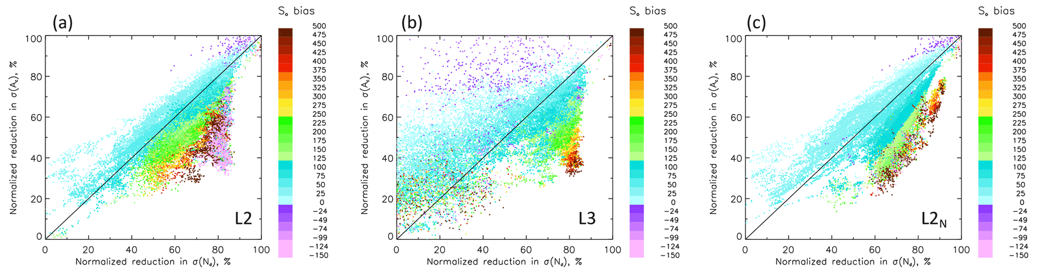
Figure 9 As in Fig. 7 but with points colored by S_o bias. Biases exceeding 100 % always occur when averaging-related smoothing has a stronger effect on N_d than on A_c.

Analysis of L3 shows some similarities to and some differences from L2. First, there is a much more significant scatter in points, particularly at lower f_c (Fig. 7b); second, as in L2, averaging-related smoothing of N_d tends to exceed smoothing in A_c at higher f_c (Fig. 7b); third, and different from L2, values of the r ratio of ≈1 (Fig. 8b, green colors) are associated with higher S_o biases (Fig. 9b), which must derive from the σ ratio.

Finally, L2_N reveals a somewhat richer palette of responses. First the commonalities: (i) the general trend for smoothing of N_d to exceed smoothing of A_c with increasing f_c and increasing r ratio is relatively robust (cf. Fig. 7a–c). (ii) When the r ratio ≈ 1 and smoothing of the fields is similar (Fig. 8a and c), the S_o bias is capped at about 100 % (Fig. 9a and c). In fact it is clear from Fig. 9 that S_o biases exceeding 100 % always occur when averaging-related smoothing has a stronger effect on N_d than on A_c, although the magnitude and even sign of these biases vary significantly depending on the methodology. The richness (lack of monotonicity) in responses under these conditions depends on the relative strength of the r ratio and the extent to which it amplifies or counteracts the σ ratio.

We note one interesting difference between L2 and L2_N: for the latter, low-f_c points reside in conditions under which averaging-related smoothing is dominated by more as well as less significant smoothing of N_d vs. A_c (Fig. 7c). In very rare cases the low-f_c points above but close to the 1:1 line in Fig. 9c cause negative S_o biases (cf. Fig. 6c). Finally, some very high positive S_o biases (up to 500 %) do exist for L2_N. These can be traced to conditions when the r ratio is large (Fig. 8c), and averaging smoothens N_d more than A_c. In this case the effects of averaging on the r ratio and the σ ratio work in unison to amplify the bias.

4.1.3 S_o bias vs. ℒ adjustment bias

The topic of ℒ adjustments is of great interest given that the term may both enhance or offset the overall albedo susceptibility (Eq. 1) (e.g., Glassmeier et al., 2021). For example, a value of ${\mathcal{L}}_{\mathrm{o}}=d\ln \mathcal{L}/d\ln N_{\mathrm{d}}<-\mathrm{0.4}$ will change the sign of S_o from positive to negative. Numerous recent articles, based on models and observations, point to ℒ_o being positive in precipitating conditions, following the familiar Albrecht (1989) “cloud lifetime” hypothesis which posits that aerosol perturbations will suppress collision–coalescence and decrease precipitation and therefore ℒ losses, while it is negative in the non-precipitating regime as a result of enhanced evaporation–entrainment feedbacks (Wang et al., 2003; Ackerman et al., 2004; Xue et al., 2008; Christensen and Stephens, 2011; Gryspeerdt et al., 2019). Figure 10 shows the relationship between spatial-averaging-related S_o and ℒ_o biases, with points colored by f_c. For clarity we show a subsample of 58 of the total 127 simulations to avoid points clustering and obscuring points below. These 58 samples represent Latin hypercube sampling of the full data set and do not exhibit any bias relative to the full set.

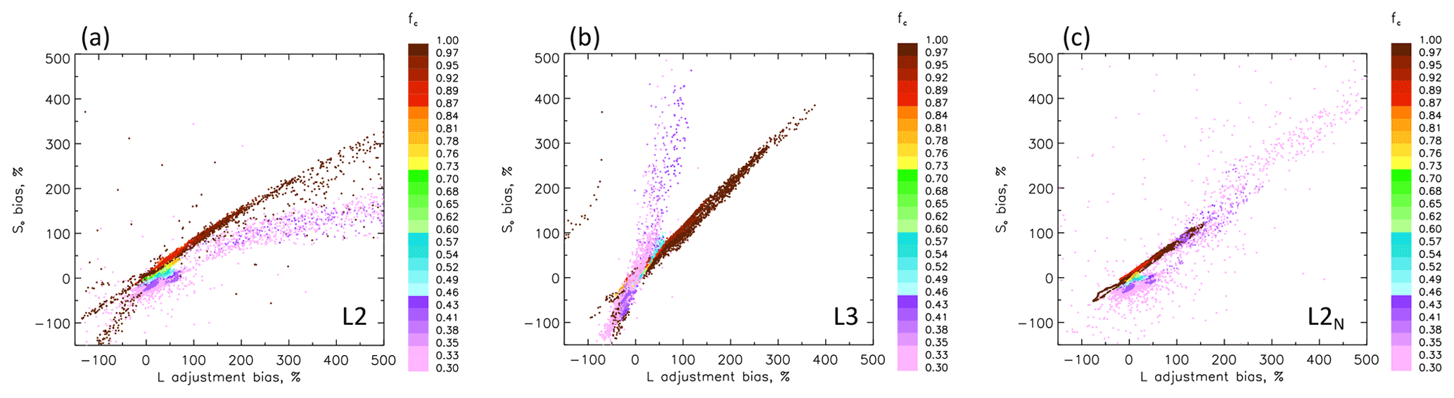
Figure 10 S_o bias vs. the ℒ adjustment bias ($d\ln \mathcal{L}/d\ln N_{\mathrm{d}}$ in Eq. 1) for a limited set of model scenes (for clarity). Note a strong positive correlation between the two biases, as expected from Eq. (1). In (a) and (b), the relative magnitude of these biases depends on f_c, although with an opposite trend. In (a) and (c), the ℒ adjustment bias tends to be larger than the S_o bias.

First, we note a strong positive correlation between the two biases, with ℒ_o biases larger than S_o biases in L2 and L2_N (Fig. 10a and c). The reverse is true for L3 (Fig. 10b). For L2 and L3, two distinct branches appear: the first is a close relationship for f_c>0.7, while the second is somewhat less well defined and associated with lower f_c. There is a saturation in the ratio for f_c on the order of 0.3 in L2 (Fig. 10a), while L3 shows a distinctly stronger S_o bias at low f_c compared to the approximately linear relationship for high f_c (Fig. 10b). Detailed analysis of this flip in the relative slope for high f_c vs. low f_c for L2 and L3 can be traced to relative differences in the degree of aggregation-related smoothing between A_c and ℒ (see Appendix B).

The separation of these branches is much less distinct for L2_N (Fig. 10c), but in general ℒ_o biases are larger than S_o biases, although to a lesser extent than in L2. The absence of a clear separation in the branches is a result of the use of the correct N_d such that cloud heterogeneities affect the biases to a similar degree. While the strong positive correlation between S_o and ℒ_o biases is not surprising given the expected close relationship between S_o and ℒ_o, it is clear that, using the methodologies applied here, satellite-based analyses of the ℒ_o bias have the potential to be at least as severe as those associated with S_o biases.

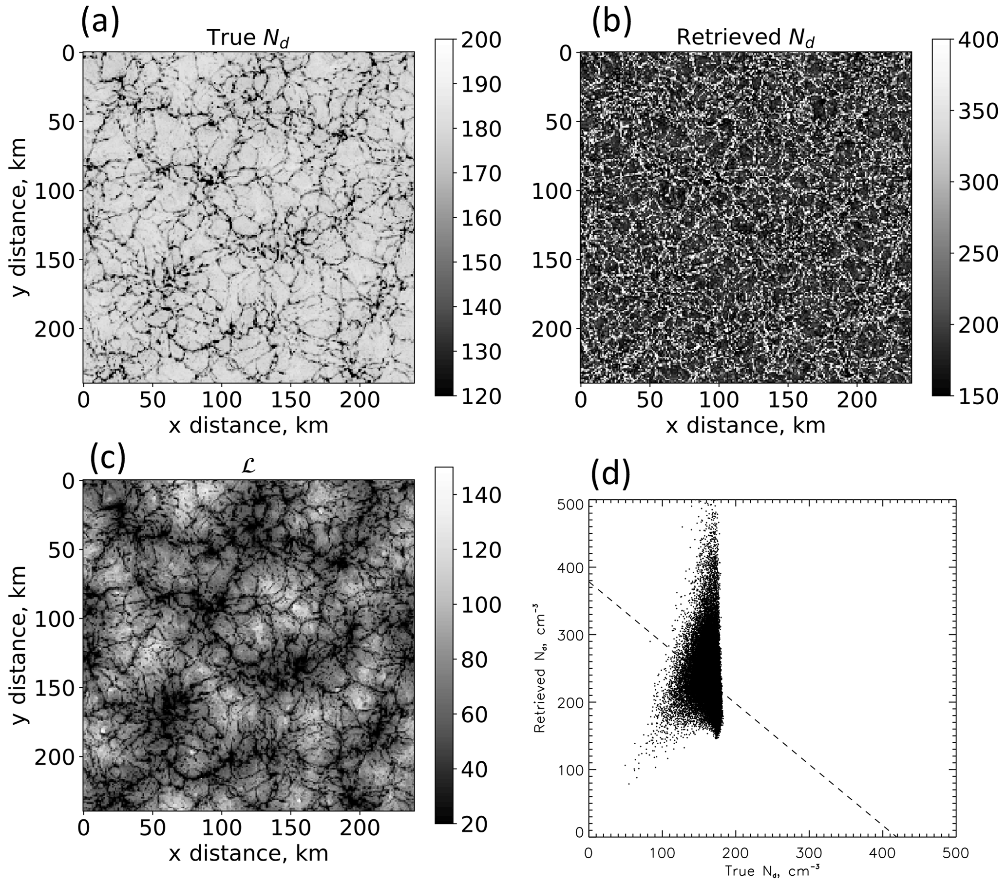
Figure 11 High-resolution (n=1) two-dimensional snapshot of (a) “true” N_d, (b) retrieved N_d (Eq. 2), (c) ℒ, and (d) the relationship between (b) and (a). Note the different scales between (a) and (b). Although the mean values of N_d in (a) and (b) differ by only −36 %, they exhibit negative correlation over the scene. The retrieved N_d introduces significant heterogeneity into the field. Use of the true N_d reduces the absolute value of the S_o error from −2017 % to +80 %.

Figure 12 As in Fig. 11 but for an open-cellular case. Note the different scales between (a) and (b). Mean values of N_d in (a) and (b) differ by −75 %. Use of the true N_d degrades the S_o bias (285 % for L2 vs. 803 % for L2_N).

4.1.4 Examples

While our goal has been to provide a broad assessment of susceptibility biases in terms of cloud field properties, some examples are helpful for illustrating the issues. We focus on L2 and L2_N to isolate the effect of the N_d retrieval for individual cases, chosen randomly based on their visual physical characteristics but supported by other cases. Figure 11 presents an LES-generated stratocumulus scene characterized by high f_c (=0.98) and a very realistic closed-cellular structure (Fig. 11a and c). Drop concentration fields for the (sub)adiabatically derived N_d, i.e., N_d,a (Eq. 2) and the “true” (LES) N_d show the problem very clearly. The retrieved N_d shows a great deal more fine-scale structure than the true N_d, and although in the mean the retrieved N_d is not highly unrealistic (retrieved N_d=167 cm⁻³; true N_d=227 cm⁻³ – an error of −26 %), the two fields are strongly negatively correlated, with a fit slope of N_d (retrieved) = $\mathrm{378}-\mathrm{0.9}\times N_{\mathrm{d}}$ (true). To quantify this further, we consider the correlations between ℒ and N_d, applying the true N_d, r(ℒ, N_d)=0.78 while using the retrieved N_d, r(ℒ, $N_{\mathrm{d}})=-\mathrm{0.24}$. This shift from strong positive r(ℒ, N_d) to negative r(ℒ, N_d) has implications for the S_o bias (e.g., Fig. 2): the L2-derived S_o bias is −2017 %, whereas the L2_N bias is +80 %. Here the use of the true N_d reduces the S_o error very significantly. This example serves to explain why high S_o biases can exist in high-f_c scenes (e.g., Fig. 4). We emphasize that the significant inhomogeneity in N_d is a result of the N_d retrieval rather than an inherent property of the cloud field and that it is this increase in inhomogeneity and reduction in r(ℒ, N_d) that drives up the S_o bias.

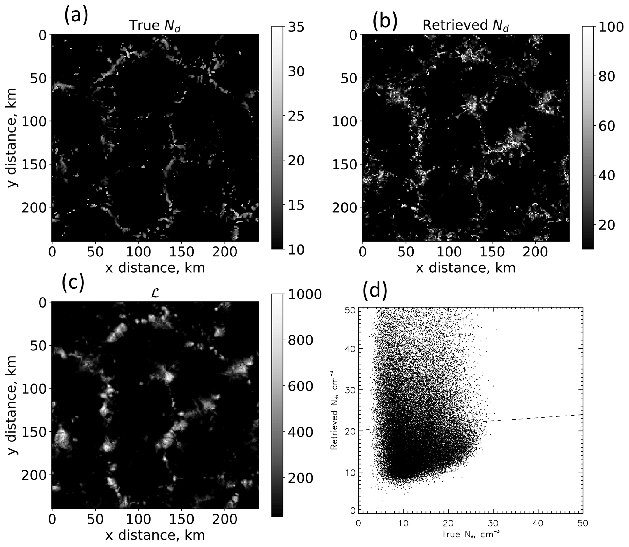
The second example (Fig. 12) is a low-f_c case (0.23) exhibiting classic open-cellular structure. Here the mean retrieved N_d is 21 cm⁻³ and the true N_d is 12 cm⁻³ – an error of +75 %. The best-fit linear regression between the two yields N_d (retrieved) = $\mathrm{20}+\mathrm{0.075}\times N_{\mathrm{d}}$ (true). Examining the true N_d, we find r(ℒ, N_d)=0.13, whereas, when using the retrieved N_d, r(ℒ, $N_{\mathrm{d}})=-\mathrm{0.05}$. The S_o biases are 285 % and 803 % for L2 and L2_N, respectively; i.e., the true N_d degrades the S_o bias. We have identified two contributing factors to this unexpected result: (i) in the case of L2_N, the proximity of r(ℒ, N_d) to zero generates an unstable r ratio and an unstable S_o bias (Eq. 13); (ii) more generally, unexpected results can occur when the base S_o (n=4) is small, which by Eq. (12) will generate unstable bias calculations. For the current case, S_o is small because the open cell walls are already very bright; i.e., 1−A_c in Eq. (1) is small.

Note that the results in Fig. 12 may seem counterintuitive at first glance since, from a satellite remote sensing perspective, a negative bias in retrieved N_d is generally expected in broken cloud scenes due to a positive bias in r_e and a negative bias in τ (e.g., Grosvenor et al., 2018). However, the aforementioned bias is a satellite-based measurement bias. In our case, we assume that r_e and τ are correct (taken directly from the model). We take the opportunity to emphasize that this work focuses on the effect of averaging cloud fields characterized by different morphologies and not with the broken cloud r_e and τ biases. The latter would need to be considered with a MODIS instrument simulator for a more complete assessment.

While examination of case studies proves useful, we argue that the broader statistical view is essential to understanding the error landscape that might be encountered in highly variable natural cloud scenes. In this regard, Figs. 3–6, supported by Figs. 7–9, are essential.

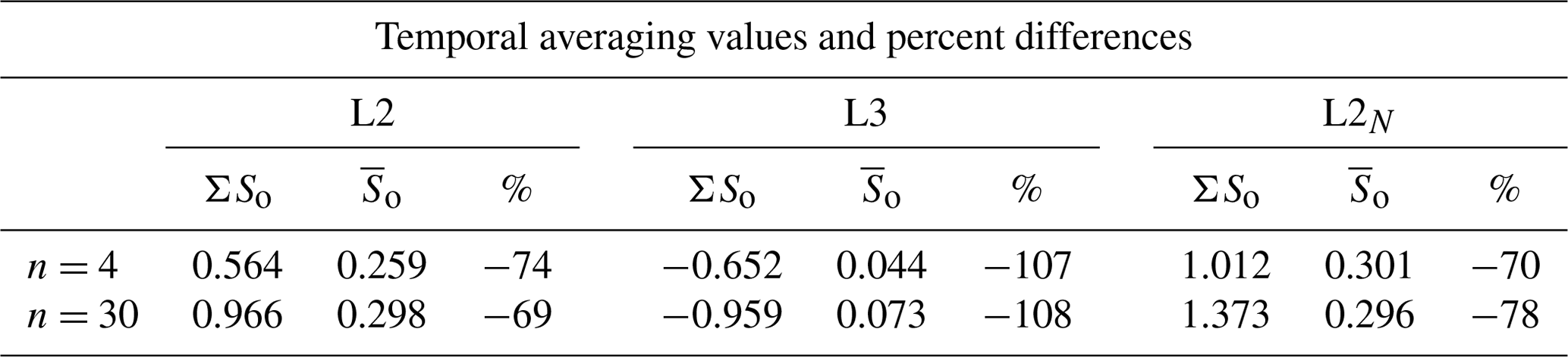
Table 1 Temporal averaging values and percent differences. ΣS_o refers to a simple average of the S_o for individual cloudy scenes. ${\stackrel{\mathrm{‾}}{S}}_{\mathrm{o}}$ refers to the S_o regression fit to the temporally aggregated data from all cloudy scenes. The percent difference is defined as (${\stackrel{\mathrm{‾}}{S}}_{\mathrm{o}}-\mathrm{\Sigma }{S}_{\mathrm{o}})/\mathrm{\Sigma }{S}_{\mathrm{o}}$. n=4 and n=30 refer to the 800 m and 6 km spatial averaging scales, respectively.

4.2 Temporal aggregation

Although the focus of the work has been on spatial aggregation, we now briefly consider the effects of temporal aggregation, which by Eq. (11) will also affect S_o. Large-scale analyses often aggregate data over multiyear timescales (e.g., Chen et al., 2014) or 3-month seasonal timescales (Lebsock et al., 2008), extending the range of conditions and changing the variance and correlation between the fields. The result is that the regression fit to a long-term, temporally aggregated data set will be different from the short timeframe fits, averaged up to include the same data.

Table 1 summarizes the results for the three methodologies (L2, L3, and L2_N) and for spatial averaging of n=4 and n=30. To represent the temporally un-aggregated approach, first a regression fit to ln A_c vs. ln N_d is performed to each scene (the entire domain) to generate a value of S_o; then the individual S_o values are averaged (represented by ΣS_o). This is done for all scenes that meet the criteria discussed in Sect. 3. The temporally aggregated approach (${\stackrel{\mathrm{‾}}{S}}_{\mathrm{o}}$) aggregates all scenes into one large data set before performing the regression. Because of the large number of individual A_c, N_d pairs required to calculate ${\stackrel{\mathrm{‾}}{S}}_{\mathrm{o}}$, calculations are limited to 58 of the 127 simulations, as in Sect. 4.1.3. The biases are calculated based on Eq. (12). Of immediate note is that the analysis shows that temporal aggregation results in a reduced S_o on the order of 70 %–110 %, depending on the methodology applied. For L2 and L2_N the average of local-in-time cloud albedo susceptibility is larger than that calculated by temporally aggregating many scenes. This bias is of opposite sign to the typical biases associated with spatial aggregation (e.g., Fig. 4) and not significantly different in magnitude. This offsetting of errors should be seen as a cautionary flag when making choices of how to aggregate data rather than as a fortuitous occurrence, since, as we have shown above, the biases are highly dependent on cloud field properties.

In the case of L3, the temporal aggregation of many different scenes results in an increase in albedo susceptibility and a change in sign from negative to weakly positive. Here too, the spatial and temporal aggregation has opposite effects (cf. Fig. 3b). (Note that the percent differences for L3 in Table 1 are somewhat misleading: because of the change in sign, increases in S_o due to temporal averaging still show up as negative differences because of the normalization by the negative ΣS_o.)

Finally, given the close relationship between the S_o and ℒ_o spatial aggregation biases, we surmise that temporal averaging will have similar effects on ℒ_o to on S_o.

5 Discussion and summary

Satellite-based measurements are our best means of assessing aerosol–cloud–radiation interactions at the global scale and providing model constraints for one of the most uncertain forcings of the atmospheric system, namely, aerosol indirect effects. Space-based data draw heavily on polar-orbiting satellites carrying passive instruments from which we infer aerosol properties (e.g., aerosol optical depth), cloud properties (cloud optical depth, cloud-top drop effective radius, liquid water path), and radiative fluxes. Typical approaches to quantification of aerosol–cloud–radiation interactions average these inferred properties spatially and temporally to suppress the “noisy” retrievals inherent to these measurements. The goal of this paper has been to address the ramifications of spatial and temporal aggregation for standard metrics of indirect effects in the form of cloud albedo susceptibility S_o, which is in turn strongly dependent on the liquid water path adjustment (ℒ_o) (Eq. 1). The question is central to our ability to quantify aerosol indirect effects and raises fundamental questions of nonlinearities in the aerosol–cloud interaction system and natural covariability of the interacting fields. Early work recognized the effects of aggregation on cloud albedo (A_c) – the so-called “albedo bias” (e.g., Cahalan et al., 1994). The current study has assumed no aggregation error in A_c (as in the case of a direct CERES-based retrieval) but has focused instead on derivatives of the form of Eq. (1) that include highly nonlinear satellite-based retrievals of drop concentration (N_d). In addition, we have derived liquid water path ℒ from the product of spectrometer-derived cloud optical depth and drop effective radius (Eq. 3), as is typically done for MODIS-based retrievals, and have not addressed the question of how this derivation might affect the S_o bias.

To provide context for the problem, we start with a theoretical framework based on spatial distributions of the interacting aerosol and cloud fields, which helps identify key variables that control the S_o bias (the variance in the fields and the correlation between the fields). Then, picking up on earlier work (McComiskey and Feingold, 2012), which analyzed three stratocumulus cloud scenes with varying degrees of cloud field variance, we extend the analysis to 127 simulations exhibiting a wide variety of stratocumulus cloud scenes. The LES provides all essential microphysical properties from which standard retrievals can be performed. The key cloud field properties are cloud-top drop effective radius r_e, cloud optical depth τ (both of which are taken directly from the LES), and A_c (based on LES τ and Eq. 4). N_d is derived from Eq. (2) and ℒ from Eq. (3). Within the framework of standard regression analysis, we quantify the effects of aggregation on the variance in the fields and the correlation between the fields and the implications for S_o biases.

The assessment of spatial aggregation biases considers three methodologies. The first is standard level-2 (L2) satellite methodology, which retrieves cloud properties at high resolution (order 1 km) and averages them up to a scale on the order of 100 km. Given the limitations in our LES domain size (40 km), we instead compare S_o based on 800 m and 6 km scales. This forms the basis of our spatial-scale averaging. Recognizing that some might choose to use the more compact aggregated data as a starting point, our second approach is level-3 (L3) methodology, which applies microphysical retrievals to spatially averaged data. Considering that a key and uncertain variable in the S_o calculation is the derived drop concentration (N_d), a third set of calculations repeats the level-2 analysis but uses the “true” (LES-calculated) N_d, which we refer to as the L2_N methodology. All consider perfect cloud albedo retrievals based on LES cloud optical depth (Eq. 4), removing the well-known cloud albedo averaging bias from the discussion. Furthermore, derived variables r_e and τ, which are central to the S_o bias analysis, have been assumed to be free of measurement error. Real-world satellite retrieval errors of these variables, especially in heterogeneous or broken cloud fields, could amplify or perhaps counter the biases identified here. Therefore, applying the conclusions directly to satellite studies should be done with caution.

Key results pertaining to spatial aggregation biases are the following.

1. S_o biases are generally positive for all three approaches and, consistent with theory, tend to increase with decreasing correlation between the fields (Fig. 4). For L2, biases can reach 500 %, whereas they are capped at about 100 % for L2_N. These biases will translate to biases in aerosol–cloud radiative forcing.

2. The L3 methodology (falsely) creates negative correlations between the cloud fields, resulting in generally unpredictable S_o bias behavior (Fig. 4b). Moreover, it generates negative S_o values (see Appendix A), exacerbated by increasing degrees of averaging (Fig. 3b). The positive S_o biases for L3 are therefore misleading (Figs. 3b and 4b).

3. High cloud fraction f_c states are equally or even more prone to S_o bias than low-f_c (high-D(ℒ)) states. This is in part due to the nature of the N_d retrieval, which introduces heterogeneity into the field (see example Fig. 11), but L2_N cases also tend to exhibit this trend. The literature tends to consider high-f_c states to be homogeneous, but this work shows that this is not necessarily the case since the N_d retrieval generates unrealistic small-scale heterogeneity in relatively homogeneous conditions.

4. Using regression theory (Eq. 11), we can interpret biases in S_o based on the extent to which averaging changes (i) the ratio of the correlation r_x,y (r ratio) and (ii) the ratio of ${\mathit{\sigma }}_y/{\mathit{\sigma }}_x$ (σ ratio) at the 6 km vs. 800 m scales. Figure 5 shows that the S_o bias is strongly dependent on the σ ratio, particularly for L3 and L2_N and for L2 at high r(ℒ, N_d). The r ratio has a weaker control over the S_o biases (Fig. 6).

5. Since the σ ratio is a ratio of ratios, we further expand our analysis of this term to assess the extent to which averaging changes ${\mathit{\sigma }}_{A_{\mathrm{c}}}$ relative to ${\mathit{\sigma }}_{N_{\mathrm{d}}}$. We find that, while averaging can reduce ${\mathit{\sigma }}_{A_{\mathrm{c}}}$ as much as ${\mathit{\sigma }}_{N_{\mathrm{d}}}$, there is a tendency for larger reductions in ${\mathit{\sigma }}_{N_{\mathrm{d}}}$ (Fig. 7), particularly for high-f_c and low r-ratio L2 cases (Fig. 8) and for low-f_c L2_N cases (Fig. 7).

6. S_o biases exceeding 100 % always occur when averaging-related smoothing has a stronger effect on N_d than on A_c (Fig. 9), although the magnitude and even sign of these biases vary significantly depending on the methodology. The lack of monotonicity in responses under these conditions depends on the relative strength of the r ratio and the extent to which it amplifies or counteracts the σ ratio. This in turn depends on the cloud fields themselves in ways that are not always easy to clarify.

7. As anticipated by Eq. (1), the S_o bias is a strong function of the ℒ_o bias (Fig. 10). In the case of L2, the ℒ_o bias is noticeably smaller than the S_o bias at low f_c, while the reverse is true for L3 (see Appendix B).

Regarding temporal aggregation, we note that if aerosol–cloud interaction metrics such as S_o are based on aggregation of cloud scenes over an extended period of time, bias can be expected as a result of extending the range of conditions beyond the natural local fluctuations inherent to covarying meteorological and aerosol conditions. To assess the effects of this temporal aggregation, we consider the difference between the average of S_o from individual cloud scenes and the S_o that is derived from a best fit to the data from all those scenes, with the former reflecting the average of local-in-time S_o and the latter reflecting the effect of temporal aggregation. Calculations are performed at both 800 m and 6 km scales (Table 1). Of note is that temporal averaging, as calculated in this manner, reduces (in percent terms) S_o at both averaging scales and for L2, L3, and L2_N analysis. The negative bias is on the order of 70 %–80 % for L2 and L2_N. As noted in Sect. 4.1.1, L3 spatial aggregation methodology generates negative S_o, and temporal aggregation has the beneficial effect of creating small positive and therefore more realistic S_o (relative to temporally un-aggregated) values. (In percentage change terms, however, the bias is negative.)

We emphasize that these offsetting effects of spatial and temporal S_o biases are very situationally dependent and require further investigation. As in the case of the regression analysis (Eq. 11) performed for spatial aggregation, the pertinent question becomes the extent to which temporal aggregation will affect the σ and r ratios. Further work will need to place this offsetting effect on firmer footing.

Finally, it is of great importance that similar assessments of S_o biases be considered in real-world satellite-based data. This will allow the community to assess the degree of coherence between the aforementioned studies and the model-based results presented here and the implications for quantification of aerosol–cloud radiative forcing.

Appendix A

Sorting or aggregation of data can generate unexpected responses. A common example of this is the relationship between “success at basketball” and “height” (Fig. A1). Although the expected positive correlation between these two variables emerges if one sorts the data by age group, the reverse occurs if one aggregates all the data together (“first aggregate, then fit”), simply because older players, while taller, do not typically perform as well as younger players. This apparent contradiction was noted by Simpson (1951) and is known as Simpson's paradox. It has received more attention during the COVID-19 pandemic as it explains apparent contradictions between vaccination rates and hospitalizations when data are not sorted by confounding factors.

Although hard to prove, the commonality for the current data is that the L2 methodology takes the approach of fitting the un-aggregated data, whereas the L3 methodology first averages the data and then performs a fit. In our case the data are not as clearly separated as in the simple example in Fig. A1, but the L2 methodology has a much higher chance of retaining the underlying physical relationship between variables than the L3 methodology. Indeed, L2 produces positive S_o, whereas L3 produces a counterintuitive negative S_o.

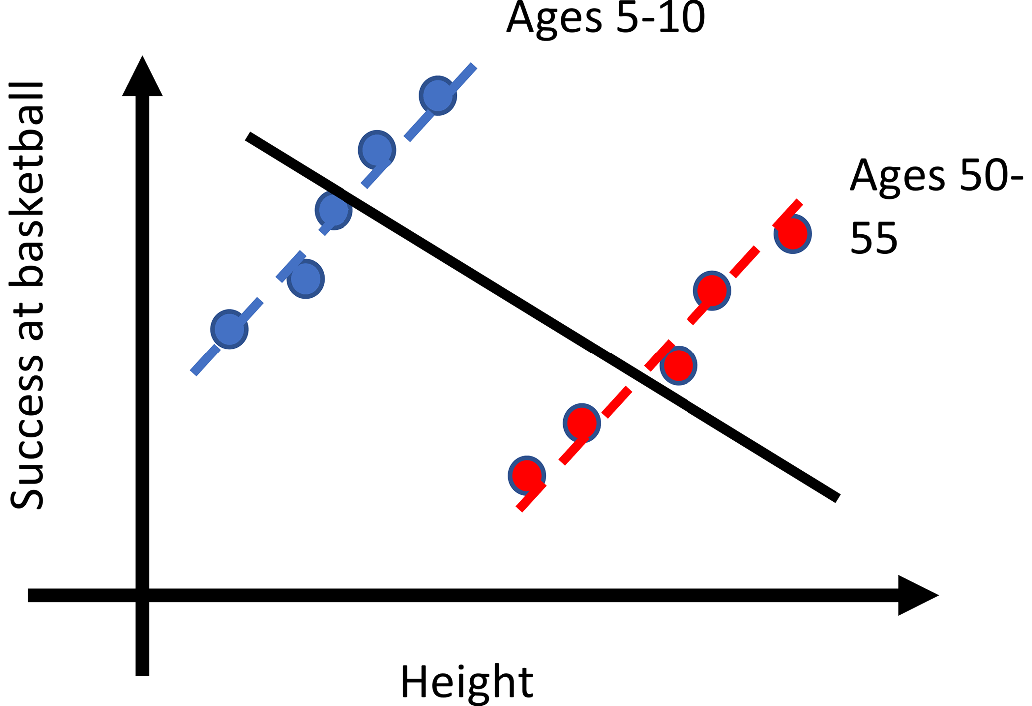
Figure A1 Demonstration of Simpson's paradox (Simpson, 1951) with the often-quoted relationship between “success at basketball” (y axis) and “height” (x axis). If data are separated by age, then the expected positive relationship emerges. If data are first aggregated, i.e., age is not taken into account, then a negative relationship emerges. The analogy to the current work is that aggregating blue points and red points separately and then fitting (as in the L3 methodology) may explain negative S_o values.

Appendix B

We address the flip in the relative slopes of low and high-f_c points for L2 and L3 in Fig. 10. Based on Fig. 7 and Eq. (13), our intuition is that it is likely a function of the change in averaging–smoothing in A_c vs. averaging–smoothing in ℒ. To test this, we repeat Fig. 7 but now also look at smoothing in ℒ and N_d.

What is apparent is that for L3, there is much more smoothing in A_c than in ℒ at low f_c (the L3 points lie closer to the 1:1 line in Fig. B1b vs. Fig. 7b for low f_c). For L2, more low-f_c points tend to lie below the 1:1 line in Fig. B1a vs. Fig. 7a, but because of this migration of points from above to below the line, it is more difficult to interpret. For L2_N the smoothing in ℒ and A_c looks similar, in line with our intuition (cf. Fig. 10, where one sees less of a bias in the relationship for low- and high-f_c points).

To dig deeper, we look more closely at the σ ratios (Eq. 13) for (i) A_c, N_d (σ ratio A_c, N_d) and (ii) ℒ, N_d (σ ratio (ℒ, N_d) for the low-f_c points. We then fit a linear relation between points for $\mathrm{0.3}<f_{\mathrm{c}}<\mathrm{0.43}$ (Fig. B2) and f_c>0.85 (not shown) and obtain the following: for $\mathrm{0.3}<f_{\mathrm{c}}<\mathrm{0.43}$, L2: $y=\mathrm{0.06}+\mathrm{0.78}x$, L3: $y=-\mathrm{0.25}+\mathrm{1.03}x$, and L2N: $y=-\mathrm{0.22}+\mathrm{1.02}x$, with x the σ ratio for ℒ and N_d and y the σ ratio for A_c and N_d. For f_c>0.85, L2: $y=\mathrm{0.1}+\mathrm{0.90}x$, L3: $y=\mathrm{0.04}+\mathrm{0.94}x$, and L2N: $y=\mathrm{0.23}+\mathrm{0.81}x$.

The high-f_c slopes for L2 and L3 are similar (0.90 vs. 0.94, respectively), but there is a more significant difference in the low-f_c slopes (0.78 vs. 1.03 for L2 and L3, respectively) and in the direction consistent with the differences between L2 and L3 (Fig. 10a and b). Note the steepening of the low-f_c points in L3 and the negative intercept for L3 at low f_c (Fig. B2), which is consistent with Fig. 10b. This points strongly to the differences in degree of aggregation-related smoothing between A_c and ℒ in these low-f_c scenes being responsible for the flip in the relative sign of S_o vs. ℒ adjustment slopes between Fig. 10a (L2) and Fig. 10b (L3).

We note that these differences in smoothing derive from the derivations of A_c (Eq. 4) and ℒ (Eq. 3), with A_c a (nonlinear) function of τ only and ℒ a function of the product of τ and r_e. Anticipating how the aggregation biases will play out is not intuitive and requires, in our experience, analyses of the kind shown here.

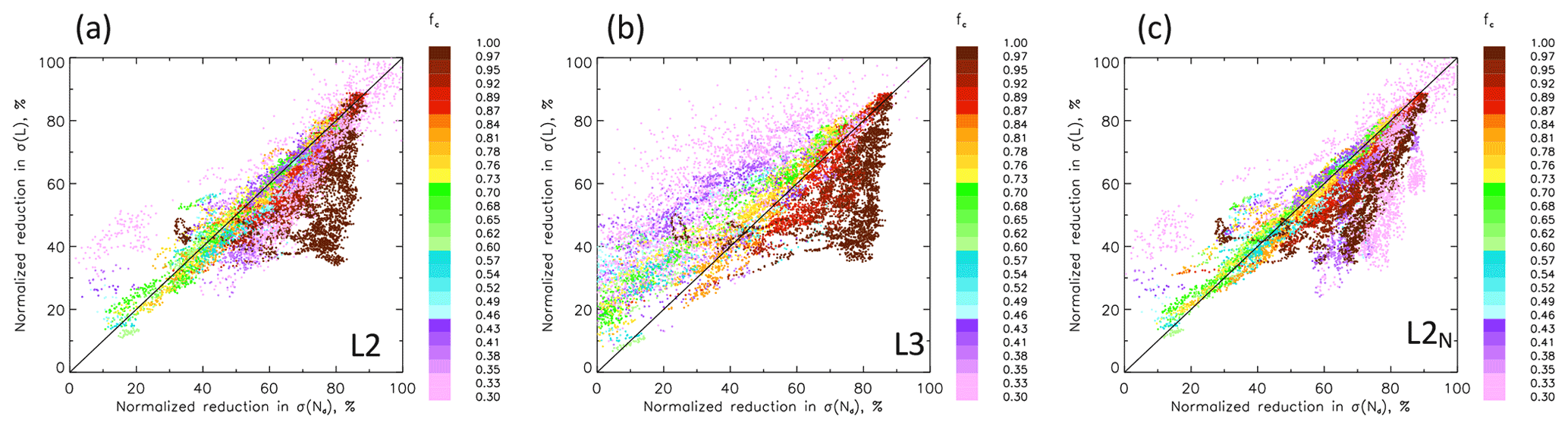
Figure B1 Effects of aggregation on normalized reduction in σ(ℒ) vs. normalized reduction in σ(N_d) to shed light on results in Fig. 10. Points are colored by f_c. In (b), and at low f_c, aggregation tends to less significantly reduce σ(ℒ) relative to σ(A_c) (Fig. 7b). (a) L2, (b) L3, and (c) L2_N. See Appendix B for further discussion.

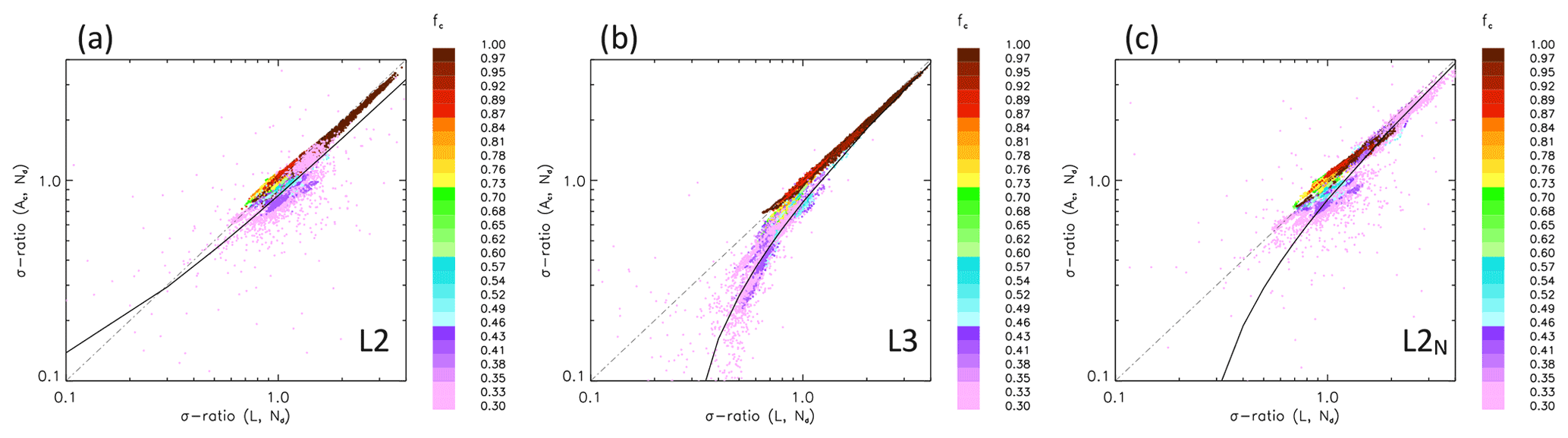
Figure B2 Plots of the σ ratio (Eq. 13) for A_c, N_d (σ ratio – A_c, N_d) vs. ℒ, N_d (σ ratio – ℒ, N_d). The solid lines are best-fit lines to the low-f_c points. The dash-dotted line is the 1:1 line. Note that the log scale distorts the solid-line linear relationships. (a) L2, (b) L3, and (c) L2_N. See Appendix B for further discussion.