A predictive viscosity model for aqueous electrolytes and mixed organic–inorganic aerosol phases

Aerosol viscosity is determined by mixture composition and temperature, with a key influence from relative humidity (RH) in modulating aerosol water content. Aerosol particles frequently contain mixtures of water, organic compounds, and inorganic ions, so we have extended the thermodynamics-based group-contribution model AIOMFAC-VISC to predict viscosity for aqueous electrolyte solutions and aqueous organic–inorganic mixtures. For aqueous electrolyte solutions, our new, semi-empirical approach uses a physical expression based on Eyring's absolute rate theory, and we define activation energy for viscous flow as a function of temperature, ion activities, and ionic strength. The AIOMFAC-VISC electrolyte model's ion-specific expressions were simultaneously fitted, which arguably makes this approach more predictive than that of other models. This also enables viscosity calculations for aqueous solutions containing an arbitrary number of cation and anion species, including mixtures that have never been studied experimentally. These predictions achieve an excellent level of accuracy while also providing physically meaningful extrapolations to extremely high electrolyte concentrations, which is essential in the context of microscopic aqueous atmospheric aerosols. For organic–inorganic mixtures, multiple mixing approaches were tested to couple the AIOMFAC-VISC electrolyte model with its existing aqueous organic model. We discuss the best-performing mixing models implemented in AIOMFAC-VISC for reproducing viscosity measurements of aerosol surrogate systems. We present advantages and drawbacks of different model design choices and associated computational costs of these methods, of importance for use of AIOMFAC-VISC in dynamic simulations. Finally, we demonstrate the capabilities of AIOMFAC-VISC predictions for phase-separated organic–inorganic particles equilibrated to observed temperature and relative humidity conditions from atmospheric balloon soundings. The predictions for the studied cases suggest liquid-like viscosities for an aqueous electrolyte-rich particle phase throughout the troposphere, yet a highly viscous or glassy organic-rich phase in the middle and upper troposphere.

1 Introduction

1.1 Viscosity and aerosols

The dynamic viscosity of various fluids and fluid mixtures is an important material property in industrial applications, cooking, and earth system science at large and small scales. The dynamic viscosity of a fluid characterizes its resistance to flow or deformation; its inverse is known as the fluidity. In the context of aerosol phases, viscosity is also important due to its relationship with the dynamics and timescales of molecular mixing and diffusion (Koop et al., 2011; Reid et al., 2018). At room temperature, liquid water has a dynamic viscosity of approximately 10⁻³ Pa s, honey one of approximately 10¹ Pa s, and pitch one of approximately 10⁸ Pa s. One can intuitively understand viscosity when attempting to pour each of these fluids out of a container: Water and honey clearly move, albeit at different speeds, while pitch is imperceptibly slow. It is useful to separate the viscosity regimes encountered in aerosol particles and other amorphous solutions into three broad categories, for example as defined by Koop et al. (2011): liquid (<10² Pa s), semi-solid (10²–10¹² Pa s), and amorphous solid or glassy (>10¹² Pa s).

Aerosols impact climate and public health. Natural and anthropogenic processes introduce immense quantities of primary and secondary aerosols into the atmosphere, including organic and elemental carbon, sulfates, nitrates, chlorides, and other inorganic material. Reactive organic compounds can form secondary organic aerosol (SOA), which can homogeneously nucleate or deposit onto preexisting aerosol (Hallquist et al., 2009; Heald and Kroll, 2020). Aerosol particles often contain a mixture of inorganic and organic matter (Zhang et al., 2007); this is especially true in urban environments (Fu et al., 2012). As relative humidity (RH) changes, organic–inorganic mixtures will uptake or release water, which changes the concentration of solutes such as inorganic electrolytes and can potentially induce liquid–liquid phase separation (LLPS) (Shiraiwa et al., 2013); in fact, the individual liquid phases could also be semi-solid or even glassy in terms of viscosity.

At very high RH (including water supersaturation), aerosol particles may uptake water to the point where they become or remain homogeneously mixed liquid-like solution droplets, while at lower RH, phase separation can occur and one or more of these phases can become relatively viscous. Such RH-dependent viscosity transitions have been observed in laboratory experiments of surrogate aerosol mixtures and reproduced in modeling studies (Reid et al., 2018). That aerosols can be highly viscous under certain conditions has raised a number of interesting questions. Does a high viscosity in an aerosol phase significantly impact the rates of heterogeneous oxidation, multiphase chemistry, or ion-displacement reactions (Zhou et al., 2019; Fard et al., 2017)? How does viscosity affect the equilibrium timescale of gas–particle partitioning for semivolatile organic compounds (Shiraiwa and Seinfeld, 2012)? Does high viscosity substantially slow the rate of water uptake and release (Wallace and Preston, 2019)? And under what environmental conditions and for which chemical compositions do we observe a glassy aerosol state (Zobrist et al., 2008; Koop et al., 2011)? Predictive viscosity models that can accommodate the varied chemistry and non-ideal behavior of aerosol mixtures should allow us to quantify these effects.

1.2 Viscosity predictions in AIOMFAC: the AIOMFAC-VISC model

Our model is contained within the Aerosol Inorganic–Organic Mixtures Functional groups Activity Coefficients (AIOMFAC) model, a group-contribution thermodynamic model which explicitly describes the interaction of organic compounds, inorganic ions, and water (Zuend et al., 2008, 2011; Yin et al., 2022). AIOMFAC-VISC, the model applied and further extended in this study, was first introduced by Gervasi et al. (2020) as a thermodynamics-based model for predicting the viscosity of aqueous organic mixtures. In this work, we extend the AIOMFAC-VISC model for the prediction of the viscosity of aqueous electrolyte solutions, obtaining a level of accuracy close to that of the engineering-oriented empirical model developed by Laliberté (2007), while using fewer parameters and a more physically justifiable equation. Moreover, we enable AIOMFAC-VISC to predict viscosity for aqueous organic–inorganic mixtures applicable to aerosol phases across the observed meteorological ranges of temperature, RH, and chemical composition. AIOMFAC-VISC refers to the full viscosity model, which comprises the electrolyte model and the organic model. This distinction becomes especially important when considering aqueous organic–inorganic mixtures. AIOMFAC can be run for specific mixture compositions and temperatures as a standalone activity coefficient model or as part of an extended equilibrium framework to compute equilibrium gas–particle partitioning, including LLPS predictions (Zuend et al., 2010; Zuend and Seinfeld, 2012; Pye et al., 2018, 2020). In the latter case, the fully developed AIOMFAC-VISC model, detailed in Sect. 2, allows for the prediction of viscosities in coexisting liquid, semi-solid, or amorphous solid phases containing water, organic compounds, and inorganic ions.

1.3 Two popular frameworks: Jones–Dole and Eyring

The two main theoretical frameworks for viscosity of aqueous electrolyte solutions are the Jones–Dole and the Eyring equations. The Jones–Dole equation is one of the earliest identified relationships for relative viscosity and is expressed as

$$\begin{array}{}\text{(1)}& {\mathit{\eta }}_{\text{rel}}={\displaystyle \frac{{\mathit{\eta }}_{\text{exp}}}{{\mathit{\eta }}_{\mathrm{0}}}}=\mathrm{1}+A\sqrt{c}+Bc,\end{array}$$

where η_rel is the relative (dynamic) viscosity, η_exp is the measured viscosity, η₀ is the pure-component viscosity of the reference solvent, c is the molarity of the dissolved electrolyte before dissociation, A is a semi-empirical constant that represents the long-range electrostatic forces between ions in solution described by Debye–Hückel theory, and B is the Jones–Dole coefficient (or sometimes simply called the B coefficient), an empirical constant that defines the contribution from short-range ion–solvent interactions to the viscosity of the solution (Jones and Dole, 1929). A and B have been calculated for many electrolytes and at many temperatures, with values available in the literature. The original Jones–Dole equation is only useful for dilute electrolyte solutions, but later extensions added parameters and terms to extend the concentration range in which it is applicable (e.g., Kaminsky, 1957; Lencka et al., 1998; Wang et al., 2004). The use of a reference electrolyte assumption can also be used to solve for ionic B coefficients. For example, KCl contains a cation and an anion of roughly the same size and charge magnitude. Therefore, the B coefficient for KCl can be evenly split into contributions for K⁺ and Cl⁻ that both equal $\frac{\mathrm{1}}{\mathrm{2}}{B}_{\mathrm{KCl}}$ (Cox et al., 1934; Kaminsky, 1957). B coefficients for many ions have been calculated using the same basic approach (Jenkins and Marcus, 1995).

Glasstone et al. (1941) introduced another equation for viscosity based on absolute rate theory, which we call the Eyring equation:

$$\begin{array}{}\text{(2)}& \mathit{\eta }={\displaystyle \frac{h{N}_{\mathrm{A}}}{V}}{e}^{\mathrm{\Delta }{g}^{\ast }/\left(RT\right)}.\end{array}$$

Here, h is the Planck constant, N_A is Avogadro's constant, R is the universal gas constant, and T is the solution temperature in kelvin (K). V is the average molar volume of the solution. The molar Gibbs energy of activation for viscous flow, Δg^∗ (units of J mol⁻¹), is a non-measurable term that can be calculated for liquids for which the viscosity is known or split into additive contributions. The Eyring equation has been tested extensively in earlier works (Goldsack and Franchetto, 1977a, b, 1978; Esteves et al., 2001; Hu and Lee, 2003; Bajić et al., 2014) and has been shown to accurately predict viscosity to higher concentrations than the Jones–Dole equation. The Eyring equation is therefore more attractive for fields that demand accurate viscosity predictions over the full range from highly dilute to highly concentrated aqueous solutions, such as applications in atmospheric aerosols.

2 Theory

2.1 Applying Eyring's basis for aqueous electrolyte viscosity in AIOMFAC-VISC

Using a known value for the viscosity of pure water, η_w, Eq. (2) becomes

$$\begin{array}{}\text{(3)}& \mathrm{\Delta }{g}_{\mathrm{w}}^{\ast }=RT\ln \left({\displaystyle \frac{{\mathit{\eta }}_{\mathrm{w}}{V}_{\mathrm{w}}}{h{N}_{\mathrm{A}}}}\right),\end{array}$$

where V_w and $\mathrm{\Delta }{g}_{\mathrm{w}}^{\ast }$ are the average molar volume and average molar Gibbs energy of activation for viscous flow of pure water. In aqueous electrolyte solutions, knowing $\mathrm{\Delta }{g}_{\mathrm{w}}^{\ast }$ and V_w allows us to solve algebraically for the Δg^∗ and V contributions of the dissolved ions. Goldsack and Franchetto (1977b) split these contributions as

$$\begin{array}{}\text{(4)}& \mathrm{\Delta }{g}^{\ast }=x_{\mathrm{w}}\mathrm{\Delta }{g}_{\mathrm{w}}^{\ast }+\sum _{i=\mathrm{1}}^J{x}_i\mathrm{\Delta }{g}_i^{\ast }\end{array}$$

and

$$\begin{array}{}\text{(5)}& V=x_{\mathrm{w}}{V}_{\mathrm{w}}+\sum _{i=\mathrm{1}}^J{x}_i{V}_i.\end{array}$$

Here, J is the number of different kinds of ions in the mixture, x_i is the mole fraction of ion i defined on the basis of dissociated ions, and x_w is the mole fraction of water. Ionic Δg^∗ contributions can be calculated, as has been previously shown for B coefficients (Goldsack and Franchetto, 1977b).

Equation (2) depends on the molar Gibbs energy of activation for viscous flow, a quantity that can be estimated but is not directly measurable. According to Eyring, viscosity can be conceptualized as the transient formation and refilling of holes in a fluid as molecules or ions diffuse through the fluid interior. This concept informs our model design. While Goldsack and Franchetto (1977b) used a modified form of the Eyring equation that emphasized binary and ternary mixtures, AIOMFAC-VISC accommodates an arbitrary number of cation and anion species in any proportion and with the added benefit of some level of predictability for aqueous electrolyte systems containing ions in combinations that have never been studied experimentally.

2.2 Deriving an expression for the molar Gibbs energy for viscous flow

Equation (2) provides an expression for mixture viscosity that depends on an effective average molar Gibbs energy of activation – see Eq. (4). Since the molar Gibbs energy of activation for viscous flow of a single ionic species, e.g., Na⁺, cannot be measured and using the reference electrolyte assumption would introduce too much uncertainty, we turn to thermodynamic theory to define an equation to estimate it. First, consider the molar Gibbs energy contribution of an ionic species to a thermodynamic phase at constant temperature and pressure, g_i=μ_i, where μ_i is the chemical potential of ion i. Analogously, we can introduce a molar Gibbs energy of activation for viscous flow, $g_i^{\ast }$. This activated-state energy can be compared to an inactivated reference state (representing equilibrium conditions), $g_i^{\text{ref}}$, such that $\mathrm{\Delta }{g}_i^{\ast }$ is defined as

$$\begin{array}{}\text{(6)}& \mathrm{\Delta }{g}_i^{\ast }=g_i^{\ast }-g_i^{\text{ref}}\end{array}$$

or, equivalently,

$$\begin{array}{}\text{(7)}& \mathrm{\Delta }{g}_i^{\ast }={\mathit{\mu }}_i^{\ast }-{\mathit{\mu }}_i^{\text{ref}}.\end{array}$$

${\mathit{\mu }}_i^{\ast }$ and ${\mathit{\mu }}_i^{\text{ref}}$ can be expressed as

$$\begin{array}{}\text{(8)}& {\mathit{\mu }}_i={\mathit{\mu }}_i^{\circ ,\left(m\right)}(p{}^{\circ },T,m{}^{\circ })+RT\ln \left[a_i^{\left(m\right)}\right],\end{array}$$

where ${\mathit{\mu }}_i^{\circ }$ is the standard-state chemical potential, and $RT\ln \left[a_i^{\left(m\right)}\right]$ is a correction term that depends on the ion activity, $a_i^{\left(m\right)}$, with superscript (m) denoting activity defined on a molality basis. For ions it is common to use a molality basis, such that the ion activity, a_i, is defined as the molality of the ion, m_i, normalized by unit molality, $m{}^{\circ }=\mathrm{1}$ mol kg⁻¹, and multiplied by the activity coefficient of the ion, γ_i (e.g., Zuend et al., 2008):

$$\begin{array}{}\text{(9)}& a_i^{\left(m\right)}={\displaystyle \frac{m_i}{m{}^{\circ }}}{\mathit{\gamma }}_i^{\left(m\right)}.\end{array}$$

Following the terminology and definition given by Yan et al. (1999), AIOMFAC defines ion molality as moles of dissociated ion per 1 kg of solvent mixture (water plus organics) as opposed to per 1 kg of water, and this must be taken into account when organics are present. For the sake of simpler notation, we will hereafter omit superscript (m) as molality basis will consistently be used for all ions in this work. Equation (7) then becomes

$$\begin{array}{}\text{(10)}& \mathrm{\Delta }{g}_i^{\ast }={\mathit{\mu }}_i^{\circ ,\ast }+RT\ln \left[a_i^{\ast }\right]-{\mathit{\mu }}_i^{\circ ,\text{ref}}+RT\ln \left[a_i^{\text{ref}}\right].\end{array}$$

During viscous flow, the standard-state chemical potential does not change, and we define ${\mathit{\mu }}_i^{\circ ,\ast }={\mathit{\mu }}_i^{\circ ,\text{ref}}$. Therefore, Eq. (10) simplifies to

$$\begin{array}{}\text{(11)}& \mathrm{\Delta }{g}_i^{\ast }=RT\ln \left[a_i^{\ast }\right]-RT\ln \left[a_i^{\text{ref}}\right]\end{array}$$

or, simpler still,

$$\begin{array}{}\text{(12)}& {\displaystyle \frac{\mathrm{\Delta }{g}_i^{\ast }}{RT}}=\ln \left({\displaystyle \frac{a_i^{\ast }}{a_i^{\text{ref}}}}\right).\end{array}$$

The problem shifts from defining the molar Gibbs energy for viscous flow to quantifying the activation activity for viscous flow. It is assumed that this special activity $a_i^{\ast }$ is a function of the reference activity, $a_i^{\text{ref}}$. Therefore, $a_i^{\ast }=f\left(a_i^{\text{ref}}\right)$, which by Eq. (9) implies dependence on ${\mathit{\gamma }}_i^{\text{ref}}$ and the molality, m_i. Thus, $\mathrm{\Delta }{g}_i^{\ast }/\left(RT\right)=f({\mathit{\gamma }}_i^{\text{ref}},m_i)$.

2.3 Contributions to Gibbs energy for viscous flow

In our model, this energy is decomposed into three component-specific, additive contributions. First, the energy required for solvent molecules to move from their original locations into vacant holes, or to form new holes, is the molar Gibbs energy for viscous flow of the solvent, $\mathrm{\Delta }{g}_{\mathrm{w}}^{\ast }$. Here we focus on water as the only solvent of ions for the purpose of this part of the AIOMFAC-VISC model for aqueous electrolyte solutions; mixtures of water, organics, and ions will be considered in Sect. 3.4. Second, the energy required for dissolved ions to move from their original locations into vacant holes is the molar Gibbs energy for viscous flow of the ions, $\mathrm{\Delta }{g}_i^{\ast }$. Third, in highly concentrated solutions, cations and anions can interact sufficiently frequently that they can impact the viscosity of the solution. The energy required for temporarily coupled cation–anion entities to move from their original locations into vacant holes is the molar Gibbs energy for viscous flow for cation–anion pairs, $\mathrm{\Delta }{g}_{c,a}^{\ast }$. Finally, Eq. (3) is used to define the molar activation energy for viscous flow for water.

2.3.1 Gibbs energy contributions from ions and cation–anion pairs

Each individual ion is assigned two coefficients, c_0,i and c_1,i, and we express $\mathrm{\Delta }{g}_i^{\ast }/\left(RT\right)$ by the functional form

$$\begin{array}{}\text{(13)}& {\displaystyle \frac{\mathrm{\Delta }{g}_i^{\ast }}{RT}}=c_{\mathrm{0},i}\ln \left(a_i^{\text{ref}}\right)+c_{\mathrm{1},i}.\end{array}$$

Here, $a_i^{\text{ref}}$ is considered to be the molal ion activity for the given mixture composition, e.g., computed with AIOMFAC. Initial tests indicated that the use of a single fit parameter per ion would provide inadequate flexibility for the model to fit experimental data, so a second parameter was included in Eq. (13). In our approach, we have no need for a reference electrolyte assumption, as molar Gibbs energy for viscous flow is defined for each ion and not each electrolyte. Note that Eq. (13) is consistent with the functional form of Eq. (12); we can write the right-hand side of Eq. (13) equivalently as $\ln \left[\right(a_i^{\text{ref}}{)}^{c_{\mathrm{0},i}}\cdot \exp \left(c_{\mathrm{1},i}\right)]$, and comparison to Eq. (12) identifies $a_i^{\ast }$ as $a_i^{\ast }=(a_i^{\text{ref}}{)}^{c_{\mathrm{0},i}+\mathrm{1}}\cdot \exp (c_{\mathrm{1},i})$. The partial or apparent hydration of certain ions in aqueous solutions is accounted for in a simplified manner when activity coefficients are computed with AIOMFAC. This is achieved by adjustments to the relative van der Waals volume and surface area values of affected ions, as detailed in Table 1 and in Zuend et al. (2008). Therefore, hydration effects are indirectly represented in the viscosity calculations via the ion activities and the ion contributions to the mean molar volume of a solution (Eq. 5); see also Sect. 2.4. Each cation–anion pair is assigned a single coefficient, c_c,a, and $\mathrm{\Delta }{g}_{c,a}^{\ast }$ is a function of the square root of molal ionic strength,

$$\begin{array}{}\text{(14)}& {\displaystyle \frac{\mathrm{\Delta }{g}_{c,a}^{\ast }}{RT}}=c_{c,a}\sqrt{I}.\end{array}$$

Molal ionic strength I is defined as

$$\begin{array}{}\text{(15)}& I={\displaystyle \frac{\mathrm{1}}{\mathrm{2}}}\sum _i^N{m}_i{z}_i^{\mathrm{2}},\end{array}$$

where m_i is the molality and z_i the integer (relative) electric charge of ion i. Equation (14) is inspired by similar expressions used for Pitzer-based ion activity coefficient expressions, such as those within AIOMFAC (Zuend et al., 2008).

2.3.2 Adding up the Gibbs energy contributions

The full expression for the molar Gibbs energy change for viscous flow of an aqueous electrolyte solution is related to Eq. (4) and fits directly into the exponential function in Eq. (2); it consists of the weighted contributions from Eqs. (3), (13), and (14), covering all individual ions and all possible binary cation–anion combinations in the solution,

$$\begin{array}{}\text{(16)}& {\displaystyle \frac{\mathrm{\Delta }{g}^{\ast }}{RT}}=x_{\mathrm{w}}{\displaystyle \frac{\mathrm{\Delta }{g}_{\mathrm{w}}^{\ast }}{RT}}+\sum _{i=\mathrm{1}}^J\left(x_i{\displaystyle \frac{\mathrm{\Delta }{g}_i^{\ast }}{RT}}\right)+\sum _{c=\mathrm{1}}^{J_c}\sum _{a=\mathrm{1}}^{J_a}\left({\mathit{\tau }}_{c,a}{\displaystyle \frac{\mathrm{\Delta }{g}_{c,a}^{\ast }}{RT}}\right).\end{array}$$

Here, τ_c,a is a special weighting term that accounts for contributions from all possible binary cation–anion pairs in a charge- and abundance-balanced manner. This can be accomplished by treating the aqueous solution as a mixture of charge-neutral cation–anion pairs, with each cation combined with each anion proportionally to the ion amounts involved. Consider the total positive charge in the aqueous electrolyte mixture, ${\sum }_{c=\mathrm{1}}^{J_c}{x}_c\cdot z_c$, which is equivalent to the total negative charge, ${\sum }_{a=\mathrm{1}}^{J_a}{x}_a\cdot \left|z_a\right|$, for an overall charge-neutral solution. We can define the charge fraction ψ_a as the absolute amount of charge contributed by anion a relative to the sum of absolute charge contributions of all negative charges present (or, alternatively, relative to the sum of all positive ones) in the mixture,

$$\begin{array}{}\text{(17)}& {\mathit{\psi }}_a={\displaystyle \frac{x_a\cdot \left|z_a\right|}{{\sum }_{a^{\prime }=\mathrm{1}}^{J_a}{x}_{a^{\prime }}\cdot \left|z_{a^{\prime }}\right|}},\end{array}$$

and the weighting term,

$$\begin{array}{}\text{(18)}& {\mathit{\tau }}_{c,a}={\displaystyle \frac{x_c}{{\mathit{\nu }}_{c,\text{el}}}}\cdot {\mathit{\psi }}_a.\end{array}$$

τ_c,a represents the fractional amount of the hypothetical, neutral electrolyte component el consisting of cation c and anion a, where ν_c,el is the stoichiometric number of cations in a formula unit of this electrolyte. This treatment is further described in the Supplement, in Sect. S1. Temporary cation–cation and anion–anion pairs are unlikely to form to the same extent because similarly charged ions will repel each other. Pitzer models show that to a first-order approximation, those interactions can be neglected (e.g., Zuend et al., 2008).

Some considerations bear mentioning. $\mathrm{\Delta }{g}_{\mathrm{w}}^{\ast }/\left(RT\right)$ is a unitless quantity related through Eq. (3) to the viscosity of pure water. At 298.15 K, pure water has a viscosity of $\mathrm{8.9}\times {\mathrm{10}}^{-\mathrm{4}}$ Pa s, and $\mathrm{\Delta }{g}^{\ast }/\left(RT\right)=\mathrm{3.44}$. If the total Gibbs energy for viscous flow drops below this threshold, the Eyring equation will calculate a viscosity less than that of pure water. For certain aqueous electrolyte solutions that have a local viscosity minimum in the dilute range, this is a necessary condition. When $a_i^{\text{ref}}$ values are less than one, the ionic contribution can become negative, allowing $\mathrm{\Delta }{g}^{\ast }/\left(RT\right)<\mathrm{3.44}$. To avoid viscosity values that are too low, the cation–anion contribution may compensate by being positive and of larger magnitude. This interplay of viscosity contributions from water, ions, and cation–anion interactions is delicate and requires optimized coefficients. To avoid negative $\mathrm{\Delta }{g}^{\ast }/\left(RT\right)$ and nonphysical behavior, we determined that all AIOMFAC-VISC coefficients should be positive real numbers.

2.4 Representing volume, charge, and hydration effects on viscosity

The effective size of the dissolved ions impacts the amount of Gibbs energy needed to activate viscous flow. Conceptually, if ions have small volumes, they slip relatively easily through the intermolecular network and into available/generated openings, displacing very few water molecules in the process; this would correspond to low viscosity. By contrast, large ions must displace more neighboring (solvent) molecules, which requires more energy temporarily and indicates higher viscosity. If an ion has a high charge density – the ratio of charge to ion volume – it will strongly attract water molecules into a temporary hydration shell, increasing the apparent size of the moving ion. Conversely, if an ion has low charge density, this hydration effect is reduced and is sometimes negligible. In AIOMFAC-VISC, as part of the original AIOMFAC model, hydrated volumes are used for ions, ensuring that hydration effects are included where they are important. Ions in aqueous solutions with a strong hydration effect are termed “structure-making”, while those with a large ionic volume and weak hydration effect are “structure-breaking” (Marcus, 2009). This behavior is also observed in the low-concentration mixture viscosity minimum observed in the viscosity curves of aqueous solutions of structure-breaking ions like K⁺ and ${\mathrm{NH}}_{\mathrm{4}}^{+}$ but not those of structure makers like Li⁺ and Mg²⁺ (as later shown in Fig. 2).

Molar volume of solution

We define the effective mean molar volume of the solution, V, as the mole-fraction-weighted mean of the pure-component molar volumes of the solvent and the dissolved ions, as in Eq. (5). A volume correction, c_v, is defined for the model and applied in all instances as

$$\begin{array}{}\text{(19)}& V=x_{\mathrm{w}}{V}_{\mathrm{w}}+c_v\sum _{i=\mathrm{1}}^J{x}_i{V}_i.\end{array}$$

The c_v term is included to account for potential discrepancies in attributed ionic volumes, some of which include partial hydration effects. AIOMFAC uses relative van der Waals volumes, which are calculated by solving for the volume of a sphere of radius r_c and dividing by $\mathrm{15.17}\times {\mathrm{10}}^{-\mathrm{6}}$ m³ mol⁻¹, the volume of a reference subgroup (Abrams and Prausnitz, 1975; Fredenslund et al., 1975). The reference subgroup is used to calculate relative volumes for neutral molecules as well. For example, the relative volume for H₂O is 0.92, since ($\mathrm{1.3956}\times {\mathrm{10}}^{-\mathrm{5}}$ m³ mol⁻¹$)/(\mathrm{15.17}\times {\mathrm{10}}^{-\mathrm{6}}$ m³ mol⁻¹)≈0.92. Values for the volumes and hydration numbers for the ions used in AIOMFAC-VISC are included in Table 1.

Table 1 Relative van der Waals ionic volume ($R_t^H$) parameters for cations and anions considering apparent dynamic hydration. Table adapted from Zuend et al. (2008).

^a Ionic radii, r_c, are nonhydrated. ^b Apparent dynamic hydration (ADH) effects are important for small and/or charge-dense ions. In other cases, the dynamic hydration number is zero. ^c All values are taken from Table 1 of Zuend et al. (2008) and from Table 1 of Yin et al. (2022).

3 Data and methods

3.1 Available viscosity measurements

At present, AIOMFAC can predict activity coefficients for a large number of atmospherically relevant cations and anions (Yin et al., 2022), including the seven cations (H⁺, Li⁺, Na⁺, K⁺, ${\mathrm{NH}}_{\mathrm{4}}^{+}$, Mg²⁺, Ca²⁺) and 10 anions (Cl⁻, Br⁻, ${\mathrm{NO}}_{\mathrm{3}}^{-}$, ${\mathrm{HSO}}_{\mathrm{4}}^{-}$, ${\mathrm{SO}}_{\mathrm{4}}^{\mathrm{2}-}$, I⁻, ${\mathrm{CO}}_{\mathrm{3}}^{\mathrm{2}-}$, ${\mathrm{HCO}}_{\mathrm{3}}^{-}$, OH⁻, ${\mathrm{IO}}_{\mathrm{3}}^{-}$) considered for this study. Therefore, we used viscosity measurements for aqueous electrolyte systems that included combinations of these ions. Fifty-three such systems were identified and used to fit the model. Ongoing work is extending AIOMFAC for additional ions of special relevance to aerosol particles, and future versions of AIOMFAC-VISC may include these ions. Bulk measurements (i.e., those taken with a conventional viscometer or rheometer) for 36 binary systems were used to fit AIOMFAC-VISC, 33 of which were previously aggregated by Laliberté (2007); detailed references for these 33 systems are included in that article and its electronic supplement. Bulk data from 17 ternary and quaternary aqueous electrolyte systems were also used. Finally, three data sets of droplet-based measurements are included from Song et al. (2021) and Baldelli et al. (2016). The aggregated data include measurements at temperatures ranging from 263.15 to 427.15 K. Points at temperatures greater than 333 K were excluded from our model fit, to avoid biasing the model toward relatively high temperatures and because it is unlikely that aerosols will experience temperatures above 333 K in Earth's atmosphere. Ultimately, 7055 data points were used to fit the AIOMFAC-VISC electrolyte model.

Data availability varies considerably across systems. The systems with the most data are aqueous KCl, NaCl, LiCl, and CaCl₂ – each with more than 500 points. The mean number of data points per data set is 144, but some systems like HCl, HNO₃, and NaHSO₄ each contain fewer than 20 points. As shown in Figs. 4–8, most viscosity measurements are clustered in the dilute concentration range. In fact, less than 4 % of the viscosity measurements used to fit AIOMFAC-VISC are at mass fractions of water below 0.5. The highest available solute mass fractions for bulk measurements were for Ca(NO₃)₂, NH₄NO₃, H₂SO₄, and HIO₃, where measurements are available to mass fractions of water below 0.3 (solute mass fractions above 0.7). Some systems remain close to the viscosity of pure water throughout the concentration range, while others span multiple orders of magnitude – see the right two columns of Tables 2 and 3. Structure-breaking electrolytes can be identified where ${\log }_{\mathrm{10}}(\mathit{\eta }/\mathit{\eta }{}^{\circ }{)}_{\text{min}}$ is less than the value for pure water (−3.054 at 298 K). Ca(NO₃)₂ includes the greatest range, with bulk viscosity values between 10⁻⁴ and 10⁰ Pa s and approaching even higher values for the most concentrated solutions observed in laboratory experiments. While still in the liquid-like viscosity range, these high-concentration data are of particular interest for aerosol modeling. More recently, techniques such as poke and flow, bead mobility, and holographic optical tweezers have enabled viscosity measurements for droplets (Reid et al., 2018). Due to their small size and/or absence of contact with solid surfaces, aqueous droplets often attain concentrations of solute exceeding the bulk solubility limits, suggesting higher viscosities are likely to occur in nature (e.g., Rovelli et al., 2019; Richards et al., 2020a, b; Song et al., 2021). Viscosity measurements obtained at high electrolyte concentrations are of value for the development of models like AIOMFAC-VISC to improve and/or validate predictions in this less frequently measured composition range of atmospheric relevance.

Table 2 Data set information for bulk measurements of binary aqueous electrolyte solutions used to fit the AIOMFAC-VISC electrolyte model. All data have been aggregated by Laliberté (2007, 2009) unless otherwise noted.

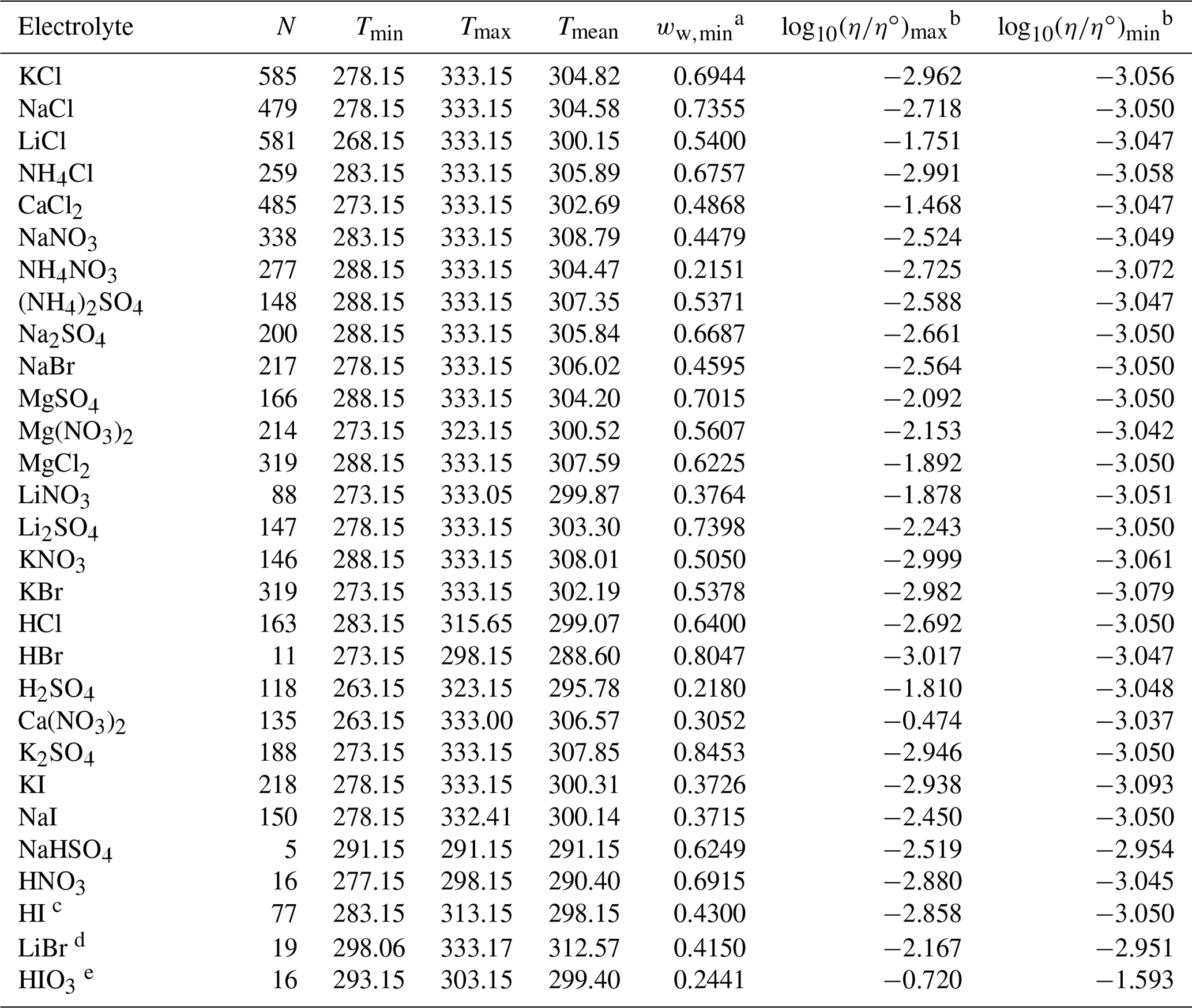
^a w_w,min is the minimum mass fraction of water, which corresponds to the highest solute concentration. ^b These columns show the maximum and minimum values for ${\log }_{\mathrm{10}}(\mathit{\eta }/\mathit{\eta }{}^{\circ })$ at $T=\mathrm{295}\pm \mathrm{5}$ K, where η^∘ denotes unit viscosity (1 Pa s). ^c Data from Nishikata et al. (1981). ^d Data from Wimby and Berntsson (1994). ^e Data from Kumar et al. (2010), including four low-concentration data points generated from the least-squares exponential fit in that article's Fig. 4.

Table 3 Data set information for bulk measurements of binary aqueous electrolyte solutions used to fit the AIOMFAC-VISC electrolyte model. All data have been aggregated by Laliberté (2007, 2009).

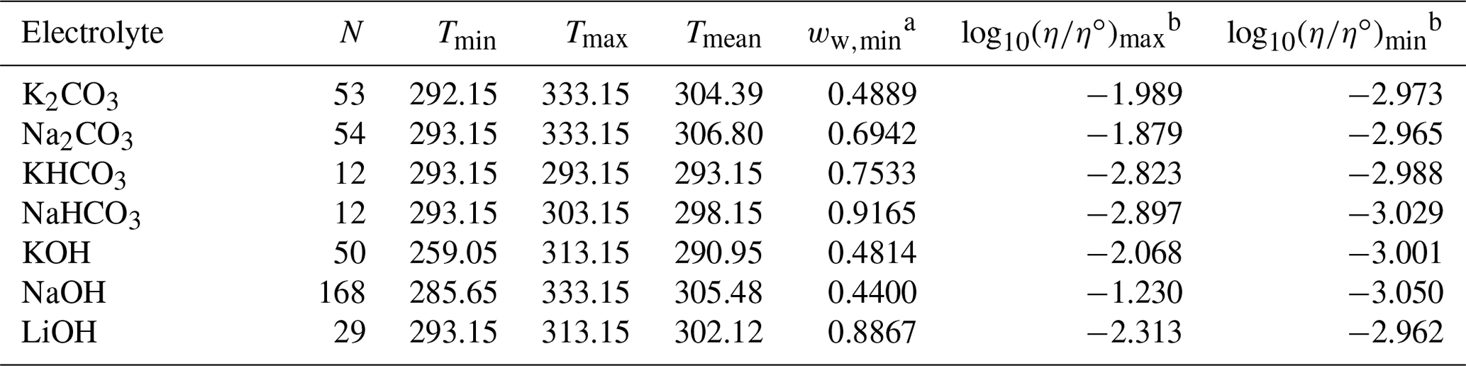
^a w_w,min is the minimum mass fraction of water, which corresponds to the highest solute concentration. ^b These columns show the maximum and minimum values for ${\log }_{\mathrm{10}}(\mathit{\eta }/\mathit{\eta }{}^{\circ })$ at $T=\mathrm{295}\pm \mathrm{5}$ K, where η^∘ denotes unit viscosity (1 Pa s).

3.1.1 Viscosity temperature dependence

Viscosity is strongly temperature dependent, and some viscosity models define their coefficients differently at each temperature, such as with the B coefficients. AIOMFAC-VISC does not do this. We posit that the temperature-dependent pure-component viscosity of water already sufficiently captures the temperature dependence of aqueous electrolyte mixtures. Moreover, the AIOMFAC-VISC coefficients are assumed to be temperature-independent. In fitting AIOMFAC-VISC, we include measurements from 263 to 333 K, and we use the same model coefficients at all temperatures. Including the data for multiple temperatures reduced the fit residuals considerably, when compared to a fit that only included data at temperatures at or near 298 K. Finally, AIOMFAC-VISC uses ion activity values from AIOMFAC that are optimized for a temperature of 298.15 K. Activity coefficients are weakly temperature dependent, so AIOMFAC-VISC predictions outside the 298±30 K range may also be less reliable. To illustrate the temperature dependence of viscosity, measurements (and AIOMFAC-VISC predictions) are shown in Fig. S14 in the Supplement for several binary aqueous electrolyte solutions at selected temperatures within the range from 268 to 328 K. It is worth noting that the commonly observed local minimum in viscosity attributed to the presence of structure-breaking electrolytes is most pronounced at lower temperatures (e.g., Fig. S14c). Since the AIOMFAC-VISC parameters are influenced by higher temperatures, our model sometimes has difficulty capturing this behavior.

3.1.2 Error in viscosity measurements

Viscosity measurement error is rarely reported for bulk measurements, especially in publications before 1990. Where values do exist, they vary widely. For example, Roy et al. (2004) claims 0.05 % error in kinematic viscosity measurements. Abdulagatov et al. (2004) describes 1.5 % error in viscosity measurements for aqueous calcium nitrate solutions. Zhang and Han (1996) describe the accuracy as within 0.05 % for their viscosity measurements of aqueous NaCl and KCl solutions. Wahab and Mahiuddin (2001) reported an error of 0.5 % for aqueous calcium chloride solutions. A proxy for viscosity error is the scatter of our training data. Viscosity values measured at the same temperature and nearly identical concentrations show considerable scatter in multiple data sets (e.g., K₂SO₄, NaNO₃, and KBr; see Fig. S14), likely owing to different measurement techniques and/or measurement, calibration, and transcription error. Laliberté (2007) found the standard deviation of their viscosity residual to be 3.7 % of the average experimental viscosity for 74 data sets consisting of over 9000 data points in total. Due to the wide range of reported errors for viscosity and the scatter among measurements at similar concentrations, we decided to treat all measurements as if they included a 2 % error. This 2 % error is also included in the objective function used to fit the model. Displayed on a logarithmic scale, this error for bulk viscosity measurements is generally smaller than the size of plotted symbols, so error bars are mostly not shown. See Tables 2–5 for information on the temperature, concentration, and viscosity ranges of these data sets. The error for droplet-based viscosity measurements is typically larger than the error in bulk measurements, in part owing to the difficulty of precisely knowing the water content of the droplets (at a certain RH) examined with these techniques.

Table 4 Data set information for bulk measurements of ternary and quaternary aqueous electrolyte mixtures used to fit the AIOMFAC-VISC electrolyte model.

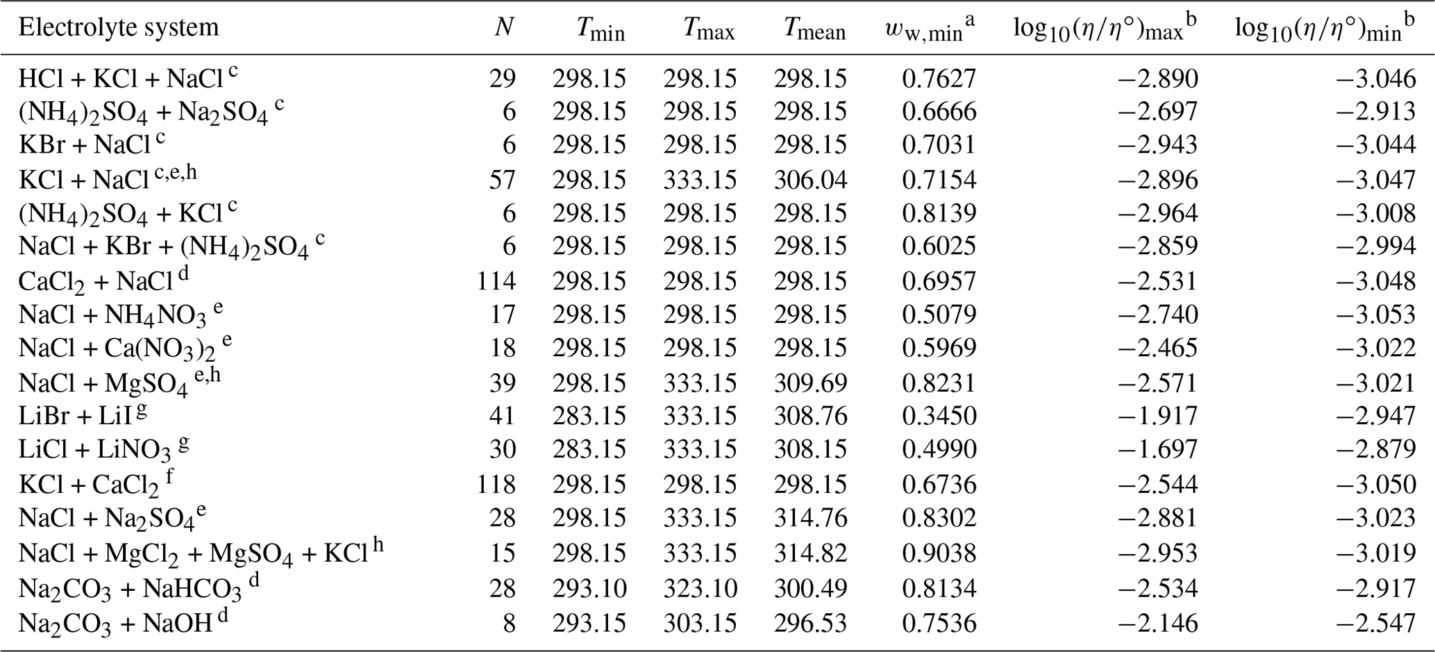
^a w_w,min is the minimum mass fraction of water, which corresponds to the highest solute concentration. ^b These columns show the maximum and minimum values for ${\log }_{\mathrm{10}}(\mathit{\eta }/\mathit{\eta }{}^{\circ })$ at $T=\mathrm{295}\pm \mathrm{5}$ K, where η^∘ denotes unit viscosity (1 Pa s). ^c Data from Goldsack and Franchetto (1977a). ^d Laliberté (2007, 2009). ^e Nowlan et al. (1980). ^f Zhang et al. (1997). ^g Iyoki et al. (1993). ^h Fabuss et al. (1969).

Table 5 Data set information for droplet-based measurements of binary aqueous electrolyte mixtures used to fit the AIOMFAC-VISC electrolyte model.

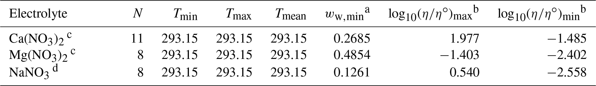
^a w_w,min is the minimum mass fraction of water, which corresponds to the highest solute concentration. For droplet-based measurements, w_w is predicted by AIOMFAC. ^b These columns show the maximum and minimum values for ${\log }_{\mathrm{10}}(\mathit{\eta }/\mathit{\eta }{}^{\circ })$ at $T=\mathrm{295}\pm \mathrm{5}$ K, where η^∘ denotes unit viscosity (1 Pa s). ^c Song et al. (2021) – poke and flow and bead mobility. ^d Baldelli et al. (2016) – holographic optical tweezers.

3.2 Simultaneously fitting the AIOMFAC-VISC electrolyte model

We used a combination of global optimization methods to simultaneously fit the c_v, c_0,i, c_1,i, and c_c,a coefficients based on the ions and cation–anion pairs described by 53 aqueous electrolyte systems. All single-ion coefficients were fitted to data from multiple systems; e.g., $c_{\mathrm{0},{\mathrm{K}}^{+}}$ and $c_{\mathrm{1},{\mathrm{K}}^{+}}$ are simultaneously fitted to all data points that include the K⁺ ion. First, we used a method described by Zuend et al. (2010) called “best-of-random differential evolution” (BoRDE), which is based on the differential evolution algorithm by Storn and Price (1997), a robust global optimization method. To implement BoRDE, we borrowed code from Zuend et al. (2010). After honing in on the coefficients with BoRDE, we switched to the constrained global optimization method (GLOBAL) by Csendes (1988), which implements the Boender–Rinnooy Kan–Stougie–Timmer algorithm in Fortran (Boender et al., 1982). The Fortran 90 version of GLOBAL is freely available online (Miller, 2003). GLOBAL identifies clusters of local minima to efficiently survey the parameter space, sometimes substantially improving upon the solution found by BoRDE. Inherent in both the GLOBAL and BoRDE fitting processes is an objective function, which is used to evaluate the model performance for a given set of the adjustable coefficients, where a smaller objective function value indicates a better model fit to the data. This function often takes the form of a residual or error equation, such as root mean square error, but it can also be customized to suit the data and the intended use of the model. Our objective function is described in Sect. 4.

3.3 Implementation for aqueous electrolyte systems

The AIOMFAC-VISC electrolyte model equations and coefficients have been implemented in Fortran and included as an optional module within the larger AIOMFAC model framework. The electrolyte model is incorporated alongside the aqueous organic viscosity model by Gervasi et al. (2020). AIOMFAC calculates activity coefficients for all components in a mixture based on activity coefficient contributions from long-range, middle-range, and short-range molecular interactions. Those three contributions include effects from dissolved ions, so it is essential that viscosity calculations for aqueous electrolyte solutions proceed after these contributions have been calculated. A number of input quantities are needed prior to calling the aqueous electrolyte solution viscosity module within AIOMFAC, including the calculation of the pure-component viscosity of water at given temperature, for which the parameterization by Dehaoui et al. (2015) is used. The mole fractions of water and the ions, the activity coefficients, and the relative ionic volumes are all available through the AIOMFAC interface, computed by various procedures within the AIOMFAC computer program. Equations (13)–(19) are then evaluated for the system, and the mixture's dynamic viscosity is calculated via Eq. (2).

3.4 Generalizing AIOMFAC-VISC: three mixing models for organic–inorganic systems

In the aerosol context, particle phases will frequently contain a mixture of water, organic compounds, and inorganic ions. Therefore, we introduce a second extension to AIOMFAC-VISC, enabling viscosity predictions for mixtures consisting of water and an arbitrary number of organic compounds and inorganic ions. We note that, to date, viscosity measurement data for organic–inorganic mixtures are scarce, limiting comparisons between model predictions and measurements and the quantitative evaluation of different mixing approaches. Given our two distinct models – the one introduced above for predicting viscosity in organic-free aqueous electrolyte solutions and the one for electrolyte-free aqueous organic mixtures (Gervasi et al., 2020) – a coupled AIOMFAC-VISC mixing model for aqueous organic–inorganic mixtures can be designed in at least three ways.

In the following sections, we introduce three approaches for combining our aqueous electrolyte and aqueous organic viscosity models and discuss their differences in terms of physicochemical justification, implementation considerations, and associated computational costs. Common to our approaches is the concept of describing the organic–inorganic system in each particle phase as a combination of two distinct subsystems: (1) an aqueous organic solution free of inorganic electrolytes and (2) an organic-free aqueous electrolyte solution. Each subsystem may contain any number of components aside from water. The split into subsystems allows us to apply the appropriate organic- or electrolyte-specific viscosity model for each subsystem. For a given overall mixture composition, there is no obvious way but several reasonable ways, by which the water content can be split into contributions to each subsystem; hence, different options emerge. Also, since water is the only common component present in the two subsystems, its modified properties (outlined in the following) can be considered to indirectly account for and mediate effects from interactions among ions and organics occurring in the actual (fully mixed) system.

3.4.1 Electrolyte-aware water mixed with organics

The first approach for computing the mixture viscosity, referred to as “aquelec”, assumes that inorganic electrolytes dissolve exclusively in water as the predominant solvent for ions, which is typically a good approximation, especially under dilute aqueous solution conditions and/or in the absence of polar organic solvents. The key idea is to replace the pure-component viscosity of water, which is used in the prediction of the mixture viscosity of the aqueous organic subsystem, with the viscosity predicted for the aqueous electrolyte subsystem. This electrolyte-aware pseudo-pure water property substitute is then applied together with the properties of the organic components in the organic model, which is based in part on combinatorial-activity-weighted contributions of water and organics to determine mixture viscosity (Gervasi et al., 2020). In the aquelec mixing approach, the following steps are taken.

1. Adjust the ion molalities, which are by default defined by the molar ion amounts relative to 1 kg of water plus organics, $m_i=n_i/(W_{\mathrm{w}}+\sum W_{\text{org}})$, to be instead redefined relative to 1 kg of pure water as solvent, where $m_{i,\text{aquelec}}=n_i/W_{\mathrm{w}}$. In these expressions, n_i is the molar amount of ion i, and W_org and W_w are the masses of organic and water components, respectively, present in the total mixture. This can be expressed using a conversion factor, λ, as follows:

   $$\begin{array}{}\text{(20)}& {\displaystyle }& {\displaystyle }{m}_{i,\text{aquelec}}=\mathit{\lambda }{m}_i,\text{(21)}& {\displaystyle }& {\displaystyle }\mathit{\lambda }={\displaystyle \frac{W_{\mathrm{w}}}{\left(W_{\mathrm{w}}+\sum W_{\text{org}}\right)}}={\displaystyle \frac{w_{\mathrm{w}}}{\left(w_{\mathrm{w}}+\sum w_{\text{org}}\right)}}.\end{array}$$

2. Using m_i,aquelec, calculate ion activities with Eq. (9) and ionic strength with Eq. (15).

3. Redefine the ionic mole fractions relative to the organic-free aqueous electrolyte subsystem (subsystem 2). The full system ionic mole fractions, $x_i=n_i/(n_w+\sum n_{\text{org}}+\sum n_i)$, are replaced by the new organic-free ionic mole fractions, $x_{i,\text{aquelec}}=x_i/(x_{\mathrm{w}}+\sum x_{i^{\prime }})$. Here, we introduce prime notation, e.g., i^′, to contrast the specific ion i with the index over which all ion molar amounts or mole fractions are summed.

4. Run the electrolyte model to calculate the viscosity of the aqueous electrolyte subsystem, ignoring organics.

5. Replace the pure-component viscosity of water in subsystem 1 with that of the aqueous electrolyte subsystem (electrolyte-aware water).

6. Set the mole fractions of ions to zero to avoid double-counting their effects and renormalize the mole fractions of water and organics for subsystem 1, so they become $x_{w,\text{aquelec}}=x_{\mathrm{w}}/(x_{\mathrm{w}}+\sum x_{{\text{org}}^{\prime }})$ and $x_{\text{org,aquelec}}=x_{\text{org}}/(x_{\mathrm{w}}+\sum x_{{\text{org}}^{\prime }})$.

7. Run the organic model (Gervasi et al., 2020) for the established mixture of electrolyte-aware water and the organic components to compute the viscosity of the organic–inorganic mixture as a whole.

3.4.2 Organics-aware water mixed with ions

As opposed to aquelec, another option, “aquorg”, assumes that all water mixes with organic components to create an organics-aware water component that will replace pure water as the solvent of ions in the organic–inorganic mixture. Unlike aquelec, which first computes the interactions between ions and pure water, aquorg prioritizes the calculation for aqueous organic mixture viscosity. This mixing model is similar to aquelec, but the steps proceed in a different order, as follows.

1. Run the organic model (Gervasi et al., 2020) to calculate the viscosity for the aqueous organic subsystem, ignoring ions.

2. Replace the pure-component viscosity property of water in subsystem 2 with that of the aqueous organic subsystem (organics-aware water).

3. Add the mole fraction values of all organics to the mole fraction of water, and set the mole fractions of all organics to zero. Thus, the sum of moles of organics plus moles of water is represented as moles of organics-aware water.

4. Run the electrolyte model for the mixture of organics-aware water and the inorganic ions to calculate viscosity of the organic–inorganic mixture.

Note that for the aquorg mixing mode, it is not necessary to modify the ion molalities because they are computed relative to 1 kg of organics-aware water, which for this purpose is equivalent to the molality definition based on mass of water plus organics in the denominator (as in the original mixture).

3.4.3 Splitting water content between organic and inorganic subsystems with a Zdanovskii–Stokes–Robinson mixing rule

The third mixing model is a Zdanovskii–Stokes–Robinson (ZSR) type mixing rule that preserves the organic-to-inorganic dry mass ratio (OIR). The ZSR mixing rule has been successfully used in many applications for the estimation of physical properties of a ternary mixture based on additive contributions from binary subsystems evaluated at the same water activity (i.e., RH under bulk equilibrium conditions) (Zdanovskii, 1936, 1948; Stokes and Robinson, 1966).

Unlike the other two mixing models described above, which only require a single call of the AIOMFAC program (for the computation of activity coefficients), the ZSR-style approach requires an iterative numerical solution: multiple runs are needed to pinpoint the mass fraction of water of the aqueous electrolyte and aqueous organic subsystems such that they yield the same water activity as that determined for the full mixture. As water activity is an output of an AIOMFAC calculation, this requires solving a non-linear equation in one unknown (mass fraction of water) for each subsystem.

Our ZSR-style mixing rule first calculates the RH of the full organic–inorganic system. Next, we split the full system into a salt-free aqueous organic subsystem (subsystem 1) and an organic-free aqueous electrolyte subsystem (subsystem 2). A modified version of Powell's hybrid method from the Fortran MINPACK library is used to calculate the water content and viscosity for the two subsystems at the target RH (Moré et al., 1980, 1984). Finally, the organic–inorganic mixture viscosity is estimated using a weighted arithmetic mean of the logarithms of subsystem viscosities, which is equivalent to a weighted geometric mean of the non-log subsystem viscosities. The expression for the mixing rule, previously described in Song et al. (2021), is

$$\begin{array}{}\text{(22)}& \ln (\mathit{\eta }/\mathit{\eta }{}^{\circ })=f_{\mathrm{1}}\ln ({\mathit{\eta }}_{\mathrm{1}}/\mathit{\eta }{}^{\circ })+f_{\mathrm{2}}\ln ({\mathit{\eta }}_{\mathrm{2}}/\mathit{\eta }{}^{\circ }),\end{array}$$

where f₁ and f₂ are the relative mass contributions from subsystem 1 and 2, respectively. η^∘ denotes unit viscosity (1 Pa s). Expressions for f₁ and f₂ must ensure that the given OIR is preserved. Consider the mass W of the full system,

$$\begin{array}{}\text{(23)}& W=W_{\text{org}}+W_{\text{el}}+W_{\mathrm{w}},\end{array}$$

where org, el, and w denote organic, electrolyte (salt), and water components, respectively. Subsystem 1 contains all of the organic mass and subsystem 2 contains all of the salt mass; the water content can be split in a way that preserves OIR. By defining the mass of the subsystems as

$$\begin{array}{}\text{(24)}& {\displaystyle }& {\displaystyle }{W}_{\mathrm{1}}=W_{\text{org},\mathrm{1}}+W_{\mathrm{w},\mathrm{1}},\text{(25)}& {\displaystyle }& {\displaystyle }{W}_{\mathrm{2}}=W_{\text{el},\mathrm{2}}+W_{\mathrm{w},\mathrm{2}},\text{(26)}& {\displaystyle }& {\displaystyle }{W}_{\text{el}}=W_{\text{el},\mathrm{2}},\text{(27)}& {\displaystyle }& {\displaystyle }{W}_{\text{org}}=W_{\text{org},\mathrm{1}},\end{array}$$

OIR can be defined as

$$\begin{array}{}\text{(28)}& \text{OIR}={\displaystyle \frac{W_{\text{org}}}{W_{\text{el}}}}={\displaystyle \frac{W_{\text{org},\mathrm{1}}}{W_{\text{el},\mathrm{2}}}}={\displaystyle \frac{w_{\text{org},\mathrm{1}}{W}_{\mathrm{1}}}{w_{\text{el},\mathrm{2}}{W}_{\mathrm{2}}}},\end{array}$$

where w_org,1 and w_el,2 are the mass fractions of the organic in subsystem 1 and salt in subsystem 2, respectively. The relative mass contributions are defined as

$$\begin{array}{}\text{(29)}& {\displaystyle }& {\displaystyle }{f}_{\mathrm{1}}={\displaystyle \frac{W_{\mathrm{1}}}{W_{\mathrm{1}}+W_{\mathrm{2}}}},\text{(30)}& {\displaystyle }& {\displaystyle }{f}_{\mathrm{2}}=\mathrm{1}-f_{\mathrm{1}}.\end{array}$$

Combining Eqs. (29) and (28), we find that

$$\begin{array}{}\text{(31)}& f_{\mathrm{1}}={\displaystyle \frac{\text{OIR}\times w_{\text{el},\mathrm{2}}}{w_{\text{org},\mathrm{1}}+\text{OIR}\times w_{\text{el},\mathrm{2}}}}.\end{array}$$

Note that f₁ and f₂ are not constant for constant OIR and must be recomputed at every RH step. In dynamic simulations, it is expected that ZSR mixing will be computationally expensive due to the multiple calls to AIOMFAC and the iterative approach.

3.4.4 Advantages and disadvantages of the different mixing models

The perfect mixing model for viscosity will be physically justifiable, efficient, and accurate. The ZSR mixing rule to determine water content is built on established thermodynamic arguments, but its implementation is computationally more expensive than the other two mixing models. The aquelec and aquorg mixing models are about equally fast because neither requires an iterative approach, but the aquelec approach seems the more reasonable choice in terms of physicochemical justification. The primary assumption of the aquelec mixing model is that ions are likely to dissolve preferentially in water. By contrast, the aquorg mixing model implicitly treats organic components similar to water in terms of acting as solvent mass for the calculations in subsystem 2, which is not always a good assumption. In terms of accuracy, recently, the ZSR mixing rule has been shown to produce reasonable predictions of viscosity within an order of magnitude of measurements (Song et al., 2021). A ZSR mixing rule likely suffices for non-reactive/non-interacting mixtures that exist as Newtonian fluids over a wide RH range. Some aqueous electrolytes and organic–inorganic mixtures, particularly those containing divalent cations, have been observed to undergo gel transitions at low RH (Cai et al., 2015; Richards et al., 2020b). Such gel phase transitions are not explicitly accounted for by AIOMFAC-VISC, and this may pose a challenge for the ZSR mixing rule. Predictions of organic–inorganic mixture viscosity with the three different approaches are compared in Sect. 4.7.

3.4.5 Activity coefficient calculations

Concurrently with the viscosity calculations, a full calculation is also carried out to determine the activity coefficients of all components/ions in the mixed organic–inorganic solution, as is also done in the absence of viscosity calculations with AIOMFAC. This is necessary because the activity coefficients of the components/ions computed for the subsystems will differ from those computed for the full system.

4 Results and discussion

Following a simultaneous fit of the AIOMFAC-VISC coefficients and implementation of the model in the AIOMFAC program, we found that AIOMFAC-VISC attained excellent agreement with bulk and droplet-based measurements and smooth extrapolations to low water contents for all 53 aqueous electrolyte systems. In this section, the values of the model parameters are reported and model design considerations are discussed first. Next, results are shown and discussed for binary, ternary, and quaternary aqueous electrolyte solutions, demonstrating the predictive capacity of the AIOMFAC-VISC aqueous electrolyte model. Finally, AIOMFAC-VISC predictions are shown for several aqueous inorganic and organic–inorganic mixtures for which recent aerosol techniques have been used to measure viscosity at target RH. The vast range of viscosities observed in nature, spanning more than 15 orders of magnitude, as well as the observed change of viscosity with composition, e.g., aerosol water content, or temperature, makes the use of a logarithmic viscosity scale useful, hence the frequent use of ${\log }_{\mathrm{10}}(\mathit{\eta }/\mathit{\eta }{}^{\circ })$ in this work.

4.1 Fitting AIOMFAC-VISC for aqueous electrolyte solutions

As discussed in Sect. 3.2, our method involved defining an objective function to fit the model. Our objective function is defined for each data set and takes the form

$$\begin{array}{}\text{(32)}& f_{\text{obj}}=\sqrt{{\displaystyle \frac{\mathrm{1}}{N}}\sum _{\mathit{\iota }=\mathrm{1}}^N{\left[\ln \left({\displaystyle \frac{{\mathit{\eta }}_{\text{calc},\mathit{\iota }}+\mathit{\sigma }\cdot {\mathit{\eta }}_{\text{exp},\mathit{\iota }}}{{\mathit{\eta }}_{\text{exp},\mathit{\iota }}+\mathit{\sigma }\cdot {\mathit{\eta }}_{\text{exp},\mathit{\iota }}}}\right)\right]}^{\mathrm{2}}},\end{array}$$

where ι is the data point index, N is the number of data points, and σ is an uncertainty threshold. Summing the f_obj values over all data sets and dividing by the sum gives the relative error contribution for each data set. Ca(NO₃)₂, HIO₃, NaNO₃, and NaOH contribute the largest shares of error, as shown in Fig. 1d. Our objective function includes a 2 % uncertainty term (σ=0.02) to characterize an approximate viscosity measurement error. However, it does not include additional consideration for the asymmetric distribution of measurements across different ranges in concentrations or temperature at which the measurements were collected, which may affect the distribution of the objective function value.

Through trial and error, we arrived at a framework that includes two coefficients per ion, one per cation–anion pair, and one volume correction term that is used for all model calculations. With the 53 aqueous electrolyte systems included in our fit, 58 unique coefficients were identified, describing 17 ions and 42 cation–anion interactions. Several c_c,a coefficients were not covered by the measured systems but can still occur in AIOMFAC-VISC predictions; therefore, coefficients from similar cation–anion pairs were substituted in these cases, serving as approximations, e.g., $c_{{\mathrm{Mg}}^{\mathrm{2}+},{\mathrm{Br}}^{-}}=c_{{\mathrm{Mg}}^{\mathrm{2}+},{\mathrm{Cl}}^{-}}$. All values of these coefficients are included in Tables 6 and 7, and replacements are noted in Table S3 in the Supplement. The fitted c_v value is 1.679827.

Table 6 AIOMFAC-VISC ion coefficients, c_0,i and c_1,i. ^a.

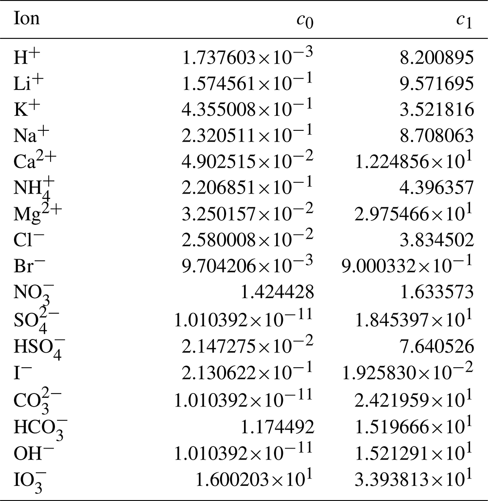
^a The number of digits listed reflects approximately the precision used in the model code; it does not imply that all digits are significant figures.

Table 7 AIOMFAC-VISC cation–anion pair coefficient, c_c,a. ^a,b.

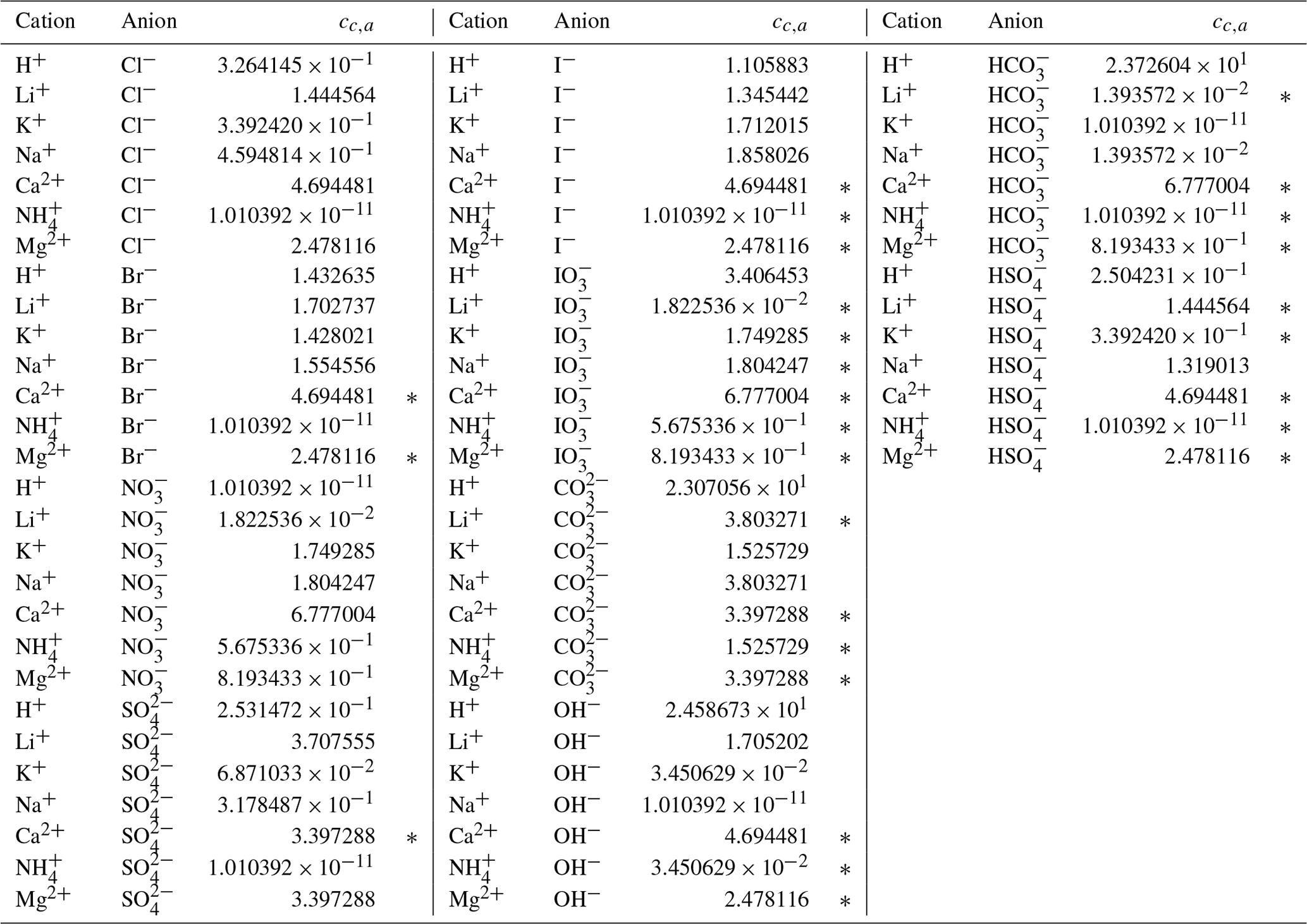
^a The number of digits listed reflects approximately the precision used in the model code; it does not imply that all digits are significant figures. ^b ∗ denotes cation–anion pairs for which no measurements were available. In these cases, the fit parameter of a similar pair is substituted; e.g., Ca²⁺ Br⁻ uses the same value as Ca²⁺ Cl⁻. See Table S3 for full list of substitutions made.

4.2 Model design considerations

How many parameters are needed to accurately and meaningfully model the viscosity of a binary aqueous electrolyte solution? The answer to this question is not so simple, as some parameters are defined for the entire model, whereas others are solute- or ion-specific. The model by Lencka et al. (1998) extends the Jones–Dole framework by including ionic B coefficients and introducing a third term for species–species interaction that is proportional to the square of molar ionic strength. It requires three parameters: two ionic B coefficients and one binary interaction parameter. As in the Jones–Dole equation, however, the B coefficients are temperature-dependent, and some aqueous electrolyte solutions require extra parameters for the species–species interaction term. By contrast, the Laliberté (2007) model uses six coefficients per electrolyte. Temperature dependence is embedded in their expression for solute viscosity, and their use of six coefficients per electrolyte is able to correlate viscosity over a broad concentration range (with limited extrapolation beyond the concentration and temperature range of available measurement data), meaning that the full flexibility of his model is contained in a single equation.

We argue that AIOMFAC-VISC is more predictive and versatile than Laliberté's model because AIOMFAC-VISC's single-ion coefficients are simultaneously fitted with data from multiple aqueous electrolyte systems and can be used to estimate viscosity in binary and multi-electrolyte systems for which no laboratory viscosity measurements exist. Furthermore, Laliberté's mixing model, a mass-fraction-weighted mixing rule, requires knowledge of the solute concentration in terms of associated electrolyte units. Atmospheric aerosols often include multiple dissociated cations and anions, as is the case with aerosolized seawater (Fabuss et al., 1969; Prather et al., 2013). In the Laliberté model, predicting the viscosity of multi-ion solutions introduces ambiguity because the ions would need to be mapped into electrolyte units. For example, an aqueous mixture of KBr and NaCl and an aqueous mixture of KCl and NaBr have different calculated viscosities according to the Laliberté model, even though the ionic concentrations are identical. AIOMFAC-VISC can sidestep this problem of electrolyte ambiguity with its unique design. A further aspect of the use of single-ion contributions to viscosity, via Eq. (13), is the dependence on predicted single-ion activities in this expression, allowing the resulting $\mathrm{\Delta }{g}_i^{\ast }$ term to indirectly account for non-ideal mixing effects. This means that effects of specific counterions on a particular ion in the solution, at otherwise the same solute molality, are considered. Therefore, while the single-ion coefficients (c_0,i and c_1,i) are the same for ion i in any mixture, the interaction effects of the reference solvent and of other ions present are at least partially accounted for.

4.3 Comparison of AIOMFAC-VISC and the Laliberté model for aqueous electrolyte systems

Due to the substantial overlap in fitted data sets, we use the Laliberté model as a benchmark for AIOMFAC-VISC, both with respect to its closeness of fit to bulk viscosity measurements and its extrapolative behavior. We fitted AIOMFAC-VISC to available bulk viscosity measurements, resulting in excellent agreement for all data sets, although that is less apparent when compared with the Laliberté model. For example, in Fig. 1, we see that in panels (b)–(d) and for all systems, AIOMFAC-VISC's error magnitude is greater than that of the Laliberté model. This is expected, because the Laliberté model is fitted to aqueous electrolyte solutions (with six specific, independent parameters for each system) as opposed to AIOMFAC-VISC, which includes ion-specific coefficients shared among many electrolyte systems. As will be shown later in Sect. 4.5, a related drawback of the Laliberté model is occasional spurious behavior when extrapolating outside of the range of available measurements. The leftmost panel displays mean bias error (MBE) for the binary systems defined in Table 2. MBE is defined as

$$\begin{array}{}\text{(33)}& \text{MBE}={\displaystyle \frac{\mathrm{1}}{N}}\sum _{\mathit{\iota }=\mathrm{1}}^N\left({\log }_{\mathrm{10}}\left[{\displaystyle \frac{{\mathit{\eta }}_{\text{calc},\mathit{\iota }}}{\mathit{\eta }{}^{\circ }}}\right]-{\log }_{\mathrm{10}}\left[{\displaystyle \frac{{\mathit{\eta }}_{\text{exp},\mathit{\iota }}}{\mathit{\eta }{}^{\circ }}}\right]\right),\end{array}$$

where N is the number of points in each data set, η_calc,ι is the calculated viscosity value of either AIOMFAC-VISC or the Laliberté model, and η_exp,ι is the viscosity value reported in the measurements at point ι. Overall, AIOMFAC-VISC does not exhibit systematic bias, with negative bias for 14 data sets and positive bias for 22 data sets. The magnitudes of MBE are generally larger for AIOMFAC-VISC than for the Laliberté model, which again is expected. One system stands out, however: Ca(NO₃)₂, which shows positive bias. This system includes some of the highest viscosity values among the available measurements (e.g., 10¹ to 10² Pa s), which is a factor in their large contributions to the overall objective function error. Ca(NO₃)₂ also includes both bulk and droplet-based measurements, and these data do not agree at low water content, leading to larger fit residuals for these systems – see Fig. 9a. It is also worth noting that the Laliberté model has its largest value of MBE for Ca(NO₃)₂, suggesting that this system is difficult to model, even when using more adjustable parameters. Figures 1b and c show mean absolute error (MAE), which is defined as

$$\begin{array}{}\text{(34)}& \text{MAE}={\displaystyle \frac{\mathrm{1}}{N}}\sum _{\mathit{\iota }=\mathrm{1}}^N\left|{\log }_{\mathrm{10}}\left[{\displaystyle \frac{{\mathit{\eta }}_{\text{calc},\mathit{\iota }}}{\mathit{\eta }{}^{\circ }}}\right]-{\log }_{\mathrm{10}}\left[{\displaystyle \frac{{\mathit{\eta }}_{\text{exp},\mathit{\iota }}}{\mathit{\eta }{}^{\circ }}}\right]\right|,\end{array}$$

and root mean square error (RMSE), which is defined as

$$\begin{array}{}\text{(35)}& \text{RMSE}=\sqrt{{\displaystyle \frac{\mathrm{1}}{N}}\sum _{\mathit{\iota }=\mathrm{1}}^N{\left({\log }_{\mathrm{10}}\left[{\displaystyle \frac{{\mathit{\eta }}_{\text{calc},\mathit{\iota }}}{\mathit{\eta }{}^{\circ }}}\right]-{\log }_{\mathrm{10}}\left[{\displaystyle \frac{{\mathit{\eta }}_{\text{exp},\mathit{\iota }}}{\mathit{\eta }{}^{\circ }}}\right]\right)}^{\mathrm{2}}}.\end{array}$$

The most significant deviations from the measurements are for Ca(NO₃)₂ and HIO₃. The values of the root mean square error and the custom objective function, Eq. (32), are presented in panels (c) and (d) of Fig. 1 and reinforce the same result.

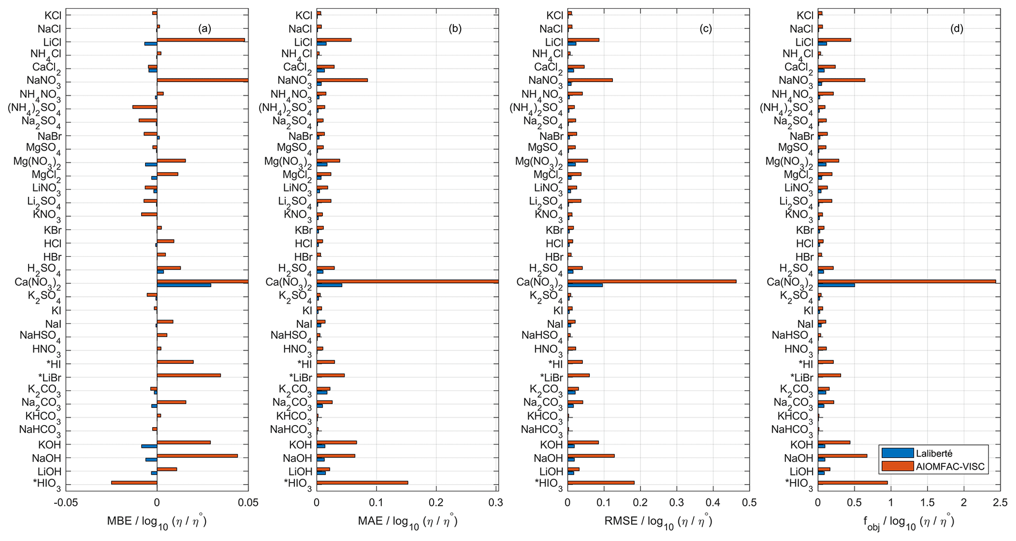
Figure 1 Comparison of AIOMFAC-VISC and the Laliberté model in terms of (a) mean bias error, (b) mean absolute error, (c) root mean square error, and (d) custom objective function value used to fit AIOMFAC-VISC. See Table 2 for information on number of data points, the ranges of temperature, concentration, and viscosity for each data set. η^∘ denotes unit viscosity (1 Pa s). Starred entries (HI, LiBr, and HIO₃) were not fitted by the Laliberté model so a model–model comparison is not possible.

In Fig. 2, the panels are zoomed in individually to show how AIOMFAC-VISC and the Laliberté model align with the bulk viscosity measurements over the covered concentration and viscosity ranges. Figures S7–S10 in the Supplement are zoomed-in versions that correspond to Figs. 5–8. KCl (Fig. 2a) and NH₄Cl (Fig. 2d) show local minima in their measured viscosity curves, a characteristic of structure-breaking electrolytes that is better captured by the Laliberté model for these systems. In these panels, as well as for NaCl (Fig. 2b), it is evident that the Laliberté model has a closer fit with the measurements. Note that the panels for KCl and NH₄Cl have extremely narrow vertical axis ranges, effectively only showing viscosities close to that of pure water. Some panels, by contrast, span more than 1 order of magnitude, with AIOMFAC-VISC agreeing well with the highest viscosity measurements. We note that if AIOMFAC-VISC is fitted only to data for an individual binary electrolyte solution, such as that for NH₄Cl shown in Fig. 2d, the model is capable of reproducing the local minimum in measured viscosity (as demonstrated in Fig. S11 in the Supplement). This indicates that the shown deviations are a result of the simultaneous fit of the model to many data sets covering a wider range in concentrations and viscosities. In Figs. 4–8, we display results for all binary aqueous electrolyte solutions, using the same limits on the vertical axes to more easily compare the viscosity ranges and extrapolations of AIOMFAC-VISC and the Laliberté model.

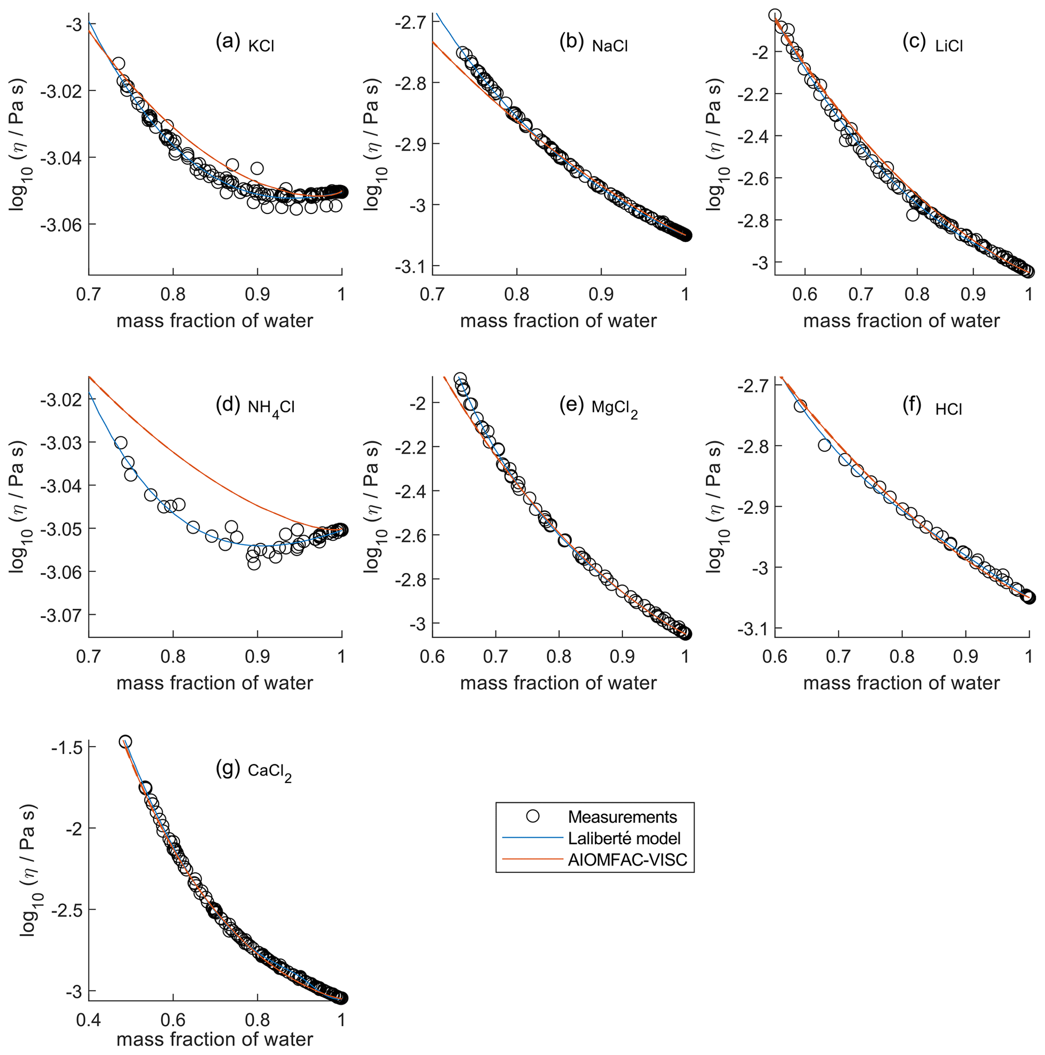
Figure 2 Comparison of closeness of fit for aqueous chloride salts/acids at 298 K with bulk measurements shown for 298±1K. Zooms are adjusted in each panel to best fit the measurement ranges. AIOMFAC-VISC model sensitivity, defined by a ± 2 % change in aerosol water content, is shown by red dashed curves. See Fig. 4 for model extrapolations throughout the full concentration range and Table 2 for information on the measurement data.

4.4 Closeness of fit to bulk viscosity measurements for ternary and quaternary aqueous electrolyte mixtures

Viscosity measurements for mixtures of water and more than one electrolyte are less common than those of binary aqueous solutions, but they better demonstrate AIOMFAC-VISC's predictive capacity. The data sets in Table 4 were used to fit AIOMFAC-VISC but were not fitted by the Laliberté model. Therefore, we effectively compare AIOMFAC-VISC's fit for these multi-ion solutions to the Laliberté mixing model, the latter being a simple mass-fraction-weighted mixing rule. As these measurements are on the same order of magnitude as the viscosity of pure water, we change the units on the vertical axis to mPa s and include 2 % error bars.

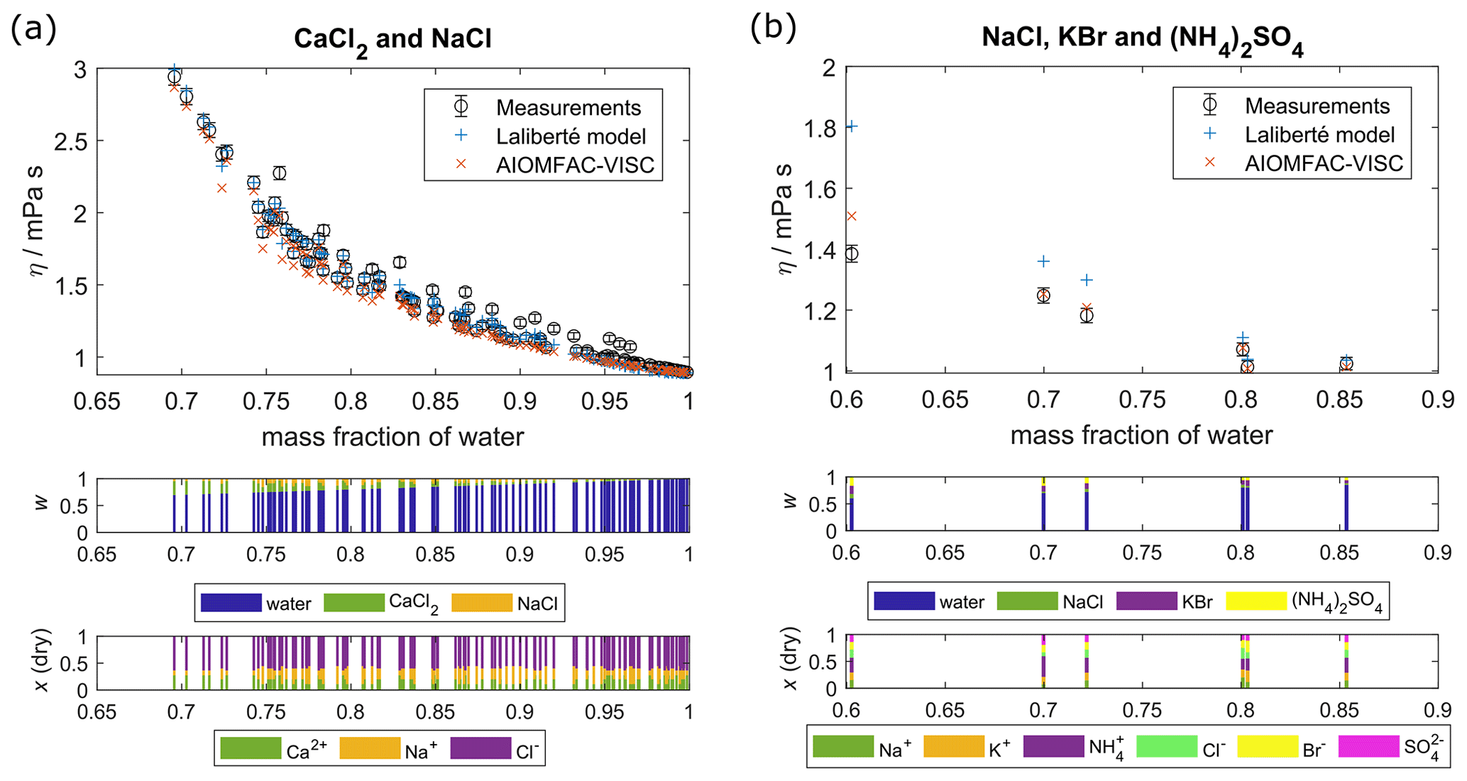
Figure 3 Comparison of AIOMFAC-VISC predictions and Laliberté model results with measured data points for aqueous mixtures of more than one electrolyte: (a) CaCl₂ and NaCl and (b) NaCl, KBr, and (NH₄)₂SO₄. Middle panel bar graphs show the mass fractions (w) with respect to non-dissociated electrolytes, and lower bar graphs show the ion mole fractions with water excluded, x(dry). The 2 % vertical error bars are included to represent viscosity measurement error.

Figure 3 shows AIOMFAC-VISC predictions alongside measurements and Laliberté-calculated values for two aqueous multi-ion solutions. As with the binary solution results, AIOMFAC-VISC and the Laliberté model agree closely at high mass fraction of water and diverge as the solute concentration increases. In Fig. 3a, there is close agreement between the two models and the measurements. This behavior is expected due to the strong model–measurement agreement of binary NaCl and binary CaCl₂. For the ternary aqueous electrolyte mixture H₂O + CaCl₂ + NaCl in Fig. 3a, the Laliberté model requires 12 parameters, or 6 for each electrolyte. AIOMFAC-VISC, by contrast, includes two coefficients for each individual ion, reducing the number needed in the case of common ions, in this case Cl⁻. For this example, AIOMFAC-VISC depends on only nine of the fitted coefficients, namely two for Ca²⁺; two for Na⁺; two for Cl⁻; one for the first cation–anion pair, Ca²⁺–Cl⁻; one for the second cation–anion pair, Na⁺–Cl⁻; and one for the volume correction term. In Fig. 3b, the number of data points is much smaller, but AIOMFAC-VISC outperforms the Laliberté model for the three points below mass fraction of water = 0.8, although both models predict slightly higher viscosities than measured. The two models perform equally well for the other three points. This is likely due to AIOMFAC-VISC's more comprehensive treatment for dissolved ions and cation–anion pairs and because we used these data during the simultaneous fit of the aqueous electrolyte model. While the Laliberté model characterizes three electrolytes and their mixing, AIOMFAC-VISC accounts for nine potential cation–anion pairs and weights their contributions in a stoichiometrically consistent way. Additional ternary and quaternary aqueous electrolyte mixtures are shown in Figs. S1–S5, located in the Supplement. In all but three of those multi-ion cases involving chloride, bromide, iodide, nitrate, sulfate, carbonate, bicarbonate, hydroxide, or any combination of these as anions, AIOMFAC-VISC performs as well or better than the Laliberté model (although this does not mean that the predictions reproduce the experimental data). The first exception is NaCl + MgSO₄ (Fig. S3a). However, the differences between the modeled viscosities in this case are less than 1 mPa s. The second is NaCl + Ca(NO₃)₂ (Fig. S1b), where AIOMFAC-VISC predicts a slightly higher viscosity than the Laliberté model for a measurement at w_w=0.6, driven by our decision to include the droplet-based measurements for aqueous Ca(NO₃)₂ in our fit, and these do not agree with the bulk measurements. The third is Na₂CO₃ + NaOH, where AIOMFAC-VISC predicts lower viscosities than measured due to underprediction of binary NaOH (Fig. S10f). Also, in several of the Supplement figures, multiple temperatures are shown, demonstrating the robustness of AIOMFAC-VISC's parameters. Given that the multi-ion data sets were used in the overall fit of the AIOMFAC-VISC parameters, this is not unexpected. Nevertheless, those successful representations of multi-ion cases, though limited by experimental data, provide confidence in AIOMFAC-VISC's ability to predict the viscosities of multi-ion solutions of various compositions.

In fitting the AIOMFAC-VISC electrolyte model, we chose to use all data sets that were available and accessible, including aqueous mixtures of more than one electrolyte. Most of the model parameters are well constrained by the binary electrolyte solution data, although two cation–anion interactions, namely ${\mathrm{NH}}_{\mathrm{4}}^{+}$–Br⁻ and Li⁺–I⁻, are fitted exclusively based on ternary mixture data because binary mixture data were not available. In comparing the performance of the AIOMFAC-VISC electrolyte model using all available data versus only binary mixture data considering overall fit quality metrics, the model improves slightly when the multi-ion data are included; see Fig. S6 in the Supplement. To further improve the model, we believe that viscosity measurements at higher electrolyte concentrations will be more helpful than measurements of multi-ion mixtures at dilute conditions. The advent of droplet-based measurements, which can probe higher concentration ranges, will be especially useful in this area. For further discussion of this, see Sect. S5 in the Supplement.

4.5 Extrapolative behavior for binary aqueous electrolyte solutions at room temperature

In Figs. 4 through 8, we compare AIOMFAC-VISC predictions with extrapolations from the Laliberté model at 298 K (or a different temperature as indicated). Agreement between AIOMFAC-VISC and the Laliberté model is excellent within the range of available measurements for each system, which are plotted as black circles. Outside of this range, the models diverge, sometimes to a large degree. It is worth noting that crystallization is inhibited/neglected in both the AIOMFAC-VISC and the Laliberté model calculations, resulting in (mostly) smooth curves throughout the concentration range. Also, the Laliberté model occasionally depicts spurious behavior outside of the measurement range. When the Laliberté model exceeds its applicability limit, which is provided for each electrolyte in Laliberté (2007), it can sometimes produce negative viscosity values as output; on a logarithmic viscosity scale plot, these deviations are indicated by a sharp discontinuity in the viscosity curve. AIOMFAC-VISC never predicts negative viscosity values, but at exceedingly low water activity, AIOMFAC by default stops its calculations when run for a single curve covering output from dilute to concentrated conditions. This is justified since the resulting water activities at low w_w would be for conditions far beyond a realistic equilibrium RH in the atmosphere (or other environments). Water activity and w_w vary differently for different aqueous electrolyte solutions as shown by comparing the upper and lower horizontal axis of each panel; so, the exact point at which the model output was stopped is different for each aqueous electrolyte solution but is typically below w_w=0.2.

Figure 4 Comparison of the Laliberté model, AIOMFAC-VISC, and viscosity measurements versus mass fraction of water (bottom axis) and AIOMFAC-predicted water activity (top axis) for binary solutions of chloride salts at 298 K with bulk measurements shown for 298±1K: (a) KCl, (b) NaCl, (c) LiCl, (d) NH₄Cl, (e) MgCl₂, (f) HCl, and (g) CaCl₂. See Fig. 2 for a zoomed-in version of this figure. Sharp discontinuities on the Laliberté model curve indicate extrapolation to non-physical values; extrapolated values should not be used beyond such points, which are outside of the valid concentration ranges provided by Laliberté (2007). AIOMFAC-VISC model sensitivity, defined by a ± 2 % change in aerosol water content, is shown in red dashed curves. AIOMFAC-VISC predictions are not shown for concentrations corresponding to exceedingly low predicted water activity ($a_{\mathrm{w}}<{\mathrm{10}}^{-\mathrm{12}}$), so the curve sometimes stops abruptly. Neither model accounts for potential crystallization of the solute (enabling predictions for extremely high ionic strengths). The values in the top axis are rounded to two significant digits. The data sources for the measurements are listed in Table 2.

Figure 5 Comparison of the Laliberté model, AIOMFAC-VISC, and viscosity measurements versus mass fraction of water (bottom axis) and AIOMFAC-predicted water activity (top axis) for binary solutions of sulfate salts at 298 K with bulk measurements shown for 298±1K unless otherwise indicated: (a) K₂SO₄, (b) Na₂SO₄, (c) Li₂SO₄, (d) (NH₄)₂SO₄, (e) MgSO₄, (f) H₂SO₄, and (g) NaHSO₄ (291 K). See Fig. S7 for a zoomed-in version of this figure. See also caption to Fig. 4.

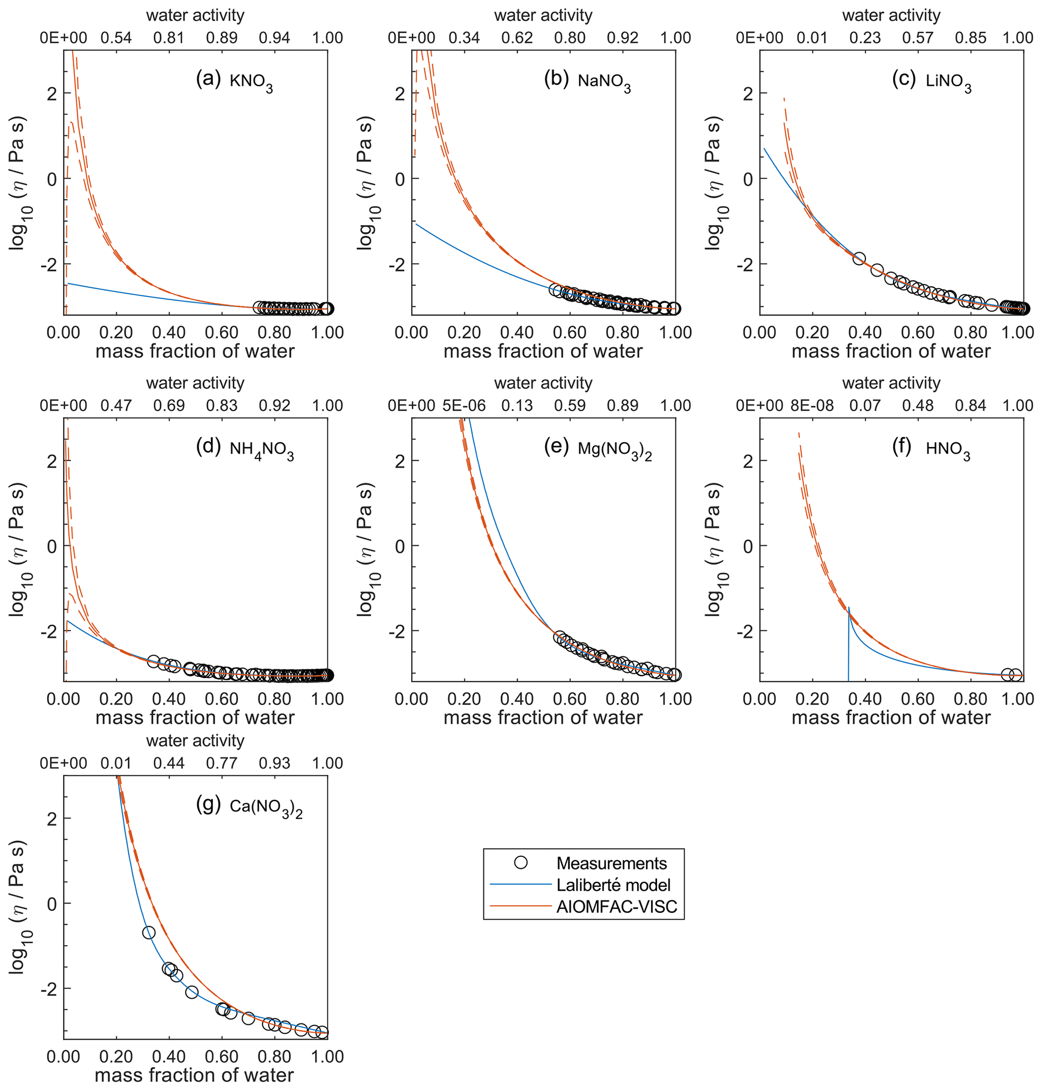
Figure 6 Comparison of the Laliberté model, AIOMFAC-VISC, and viscosity measurements versus mass fraction of water (bottom axis) and AIOMFAC-predicted water activity (top axis) for binary solutions of nitrate salts at 298 K with bulk measurements shown for 298±1K: (a) KNO₃, (b) NaNO₃, (c) LiNO₃, (d) NH₄NO₃, (e) Mg(NO₃)₂, (f) HNO₃, and (g) Ca(NO₃)₂. See Fig. 9 for comparison between bulk and droplet-based measurements for Ca(NO₃)₂, Mg(NO₃)₂, and NaNO₃. See Fig. S8 for a zoomed-in version of this figure. See also caption to Fig. 4.

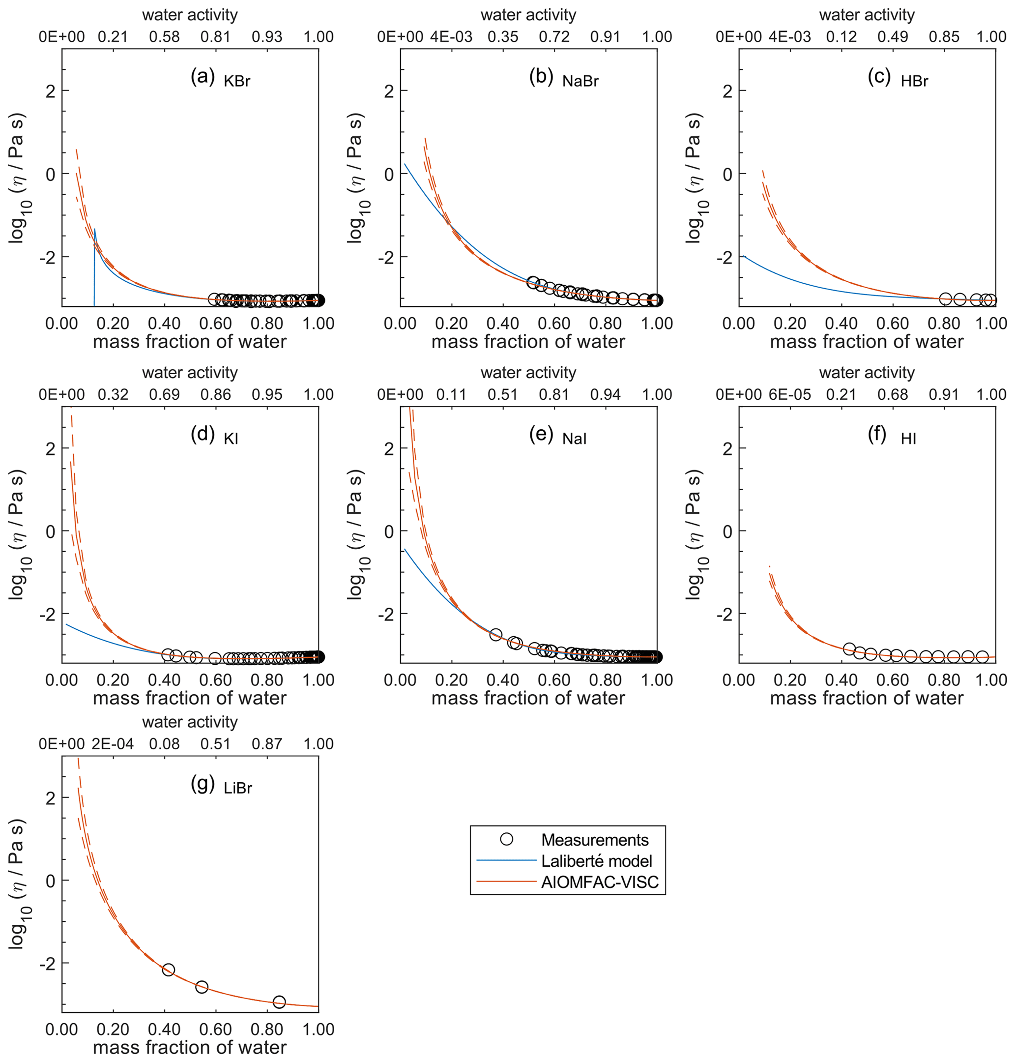
Figure 7 Comparison of the Laliberté model, AIOMFAC-VISC, and viscosity measurements versus mass fraction of water (bottom axis) and AIOMFAC-predicted water activity (top axis) for binary solutions of bromide and iodide salts at 298 K with bulk measurements shown for 298±1K: (a) KBr, (b) NaBr, (c) HBr, (d) KI, (e) NaI, (f) HI, and (g) LiBr. HI and LiBr were not fitted by the Laliberté model. See Fig. S9 for a zoomed-in version of this figure. See also caption to Fig. 4.

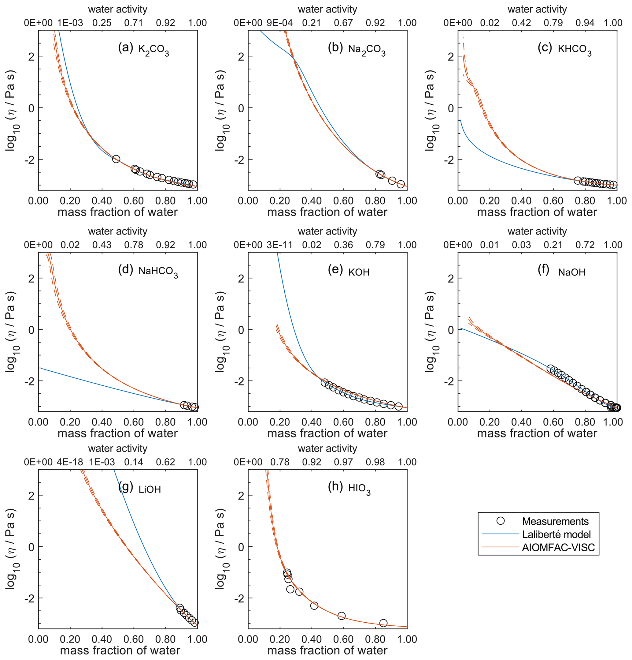
Figure 8 Comparison of the Laliberté model, AIOMFAC-VISC, and viscosity measurements versus mass fraction of water (bottom axis) and AIOMFAC-predicted water activity (top axis) for binary solutions of bromide and iodide salts at 298 K with bulk measurements shown for 298±1K unless otherwise indicated: (a) K₂CO₃, (b) Na₂CO₃, (c) KHCO₃ (293 K), (d) NaHCO₃, (e) KOH, (f) NaOH, (g) LiOH, and (h) HIO₃ (303 K). HIO₃ was not fitted by the Laliberté model. See Fig. S10 for a zoomed-in version of this figure. See also caption to Fig. 4.

For aqueous chloride salts/acids (Fig. 4), AIOMFAC-VISC and the Laliberté model agree closely, generally to within 1 order of magnitude (even outside the concentration range of the measurements). For NaCl and LiCl (Fig. 4b and c), the Laliberté model projects a near-linear increase in log ₁₀ viscosity below the w_w threshold of the measurements, while the AIOMFAC-VISC predictions include a more steep increase in viscosity below w_w=0.4, likely due to higher relative influence of the ionic-strength-dependent cation–anion viscosity contributions. For KCl, NH₄Cl, and MgCl₂ (Fig. 4a, d, and e), the Laliberté model shows spurious behavior outside of the measurement range. In these cases, the AIOMFAC-VISC predictions are preferable because the curves remain smooth.

In Figs. 5–8, AIOMFAC-VISC and the Laliberté model continue to agree closely. The AIOMFAC-VISC curve for H₂SO₄ (Fig. 5f) includes a notch below w_w=0.2, which indicates a relatively sharp change in the bisulfate dissociation degree as predicted by AIOMFAC for the sulfate–bisulfate equilibrium in that system. A similar behavior is observed for KHCO₃ (Fig. 8c) related to the dissociation of bicarbonate. For Ca(NO₃)₂ (Fig. 6g), the AIOMFAC-VISC curve closely fits the measurement points but predicts higher viscosity than the Laliberté model below w_w=0.6, due to the influence of the droplet-based measurements used to fit this system, and this is also the case for NaNO₃ (Fig. 6b) – see comparison to droplet-based measurements in Fig. 9. We also show AIOMFAC-VISC predictions for binary HI and LiBr (Fig. 7f and g) and HIO₃ (Fig. 8h), which are not fitted by the Laliberté model. Murray et al. (2012) found that HIO₃ droplets rarely effloresce, even when drying to ∼0 % RH, and that they can become highly viscous, and AIOMFAC-VISC captures this behavior.

Figure 9 Viscosity predictions for aerosol surrogate mixtures containing nitrate salts at varying water activity, a_w (RH). Model sensitivity, defined by a ± 2 % change in aerosol water content, is shown in dashed curves. Bulk measurements (see Table 2) were collected at defined concentrations and converted to a_w using AIOMFAC; the points collected at temperatures between 295±5 K are shown. Song et al. (2021) used poke-and-flow and bead mobility techniques. Baldelli et al. (2016) used holographic optical tweezers.

Due to the lack of viscosity measurements at low mass fraction of water and the tendency for salts to crystallize at high concentration, it is difficult to determine quantitatively which model/curve, if any, is correct for any given case. What is clear, however, is that AIOMFAC-VISC provides an excellent level of accuracy in the composition range where measurement data are available and can be used in place of the Laliberté model in most instances.

4.6 Comparing AIOMFAC-VISC with aqueous inorganic aerosol surrogate mixtures

Unlike bulk viscosity measurement techniques, which determine viscosity for known composition (e.g., mass fractions), recent aerosol and/or microscopic droplet viscosity measurement techniques characterize viscosity with respect to known equilibrium water activity (RH) instead. A limited number of measurements of this type are available; we present results for three aqueous nitrate salts: Ca(NO₃)₂, Mg(NO₃)₂, and NaNO₃. Measurements for aqueous NaCl from Power et al. (2013) were not available in tabulated form and not used to fit AIOMFAC-VISC, but they are shown in Fig. S13 in the Supplement.

Figure 9 shows the predicted viscosity of aqueous nitrate salts over the full RH range with AIOMFAC-VISC model sensitivity represented by the upper and lower dashed curves. AIOMFAC-VISC model sensitivity is defined by a 2 % change in the aerosol water mass fraction, described in the supporting information of Gervasi et al. (2020). In the case of aqueous Ca(NO₃)₂ (Fig. 9a), disagreement between the two measurement data sets is noticed, especially at lower water activities. AIOMFAC-VISC shows positive bias relative to the bulk measurements, and it shows better agreement with the aerosol measurements between a_w=0.65 and a_w=0.3. It is possible that these bulk measurements understate viscosity for aqueous Ca(NO₃)₂, which would mean that the large model deviation for this system is not necessarily so bad. In the case of Mg(NO₃)₂ (Fig. 9b) the aerosol measurements largely agree with the bulk measurements, and AIOMFAC-VISC correctly characterizes nearly every point. In both Fig. 9a and b there is one outlying data point at low a_w with a stated viscosity value at 10⁸ Pa s. In fact, Song et al. (2021) used 10⁸ Pa s as the upper limit for their viscosity measurements. Such a high value reported may be best explained by the crystallization of Ca(NO₃)₂ or Mg(NO₃)₂, but using the poke-and-flow measurement technique, it is difficult to distinguish between glasses, gels, and crystallized aerosols. As a result of this uncertainty, we did not include these measurements in our model fit. Crystallization is inhibited in the shown AIOMFAC-VISC predictions, likely explaining the divergence from those high-viscosity measurement points. Our AIOMFAC-based equilibrium model is capable of providing liquid–liquid and solid–liquid equilibrium calculations, but viscosity prediction would not be possible for the solid phase. In the case of NaNO₃ (Fig. 9c), there is rather poor agreement between the bulk measurements and the aerosol measurements by Baldelli et al. (2016). At a_w<0.2, the uncertainty of the AIOMFAC-VISC prediction for NaNO₃ widens considerably, indicating that small changes in solution water content can greatly affect both the water activity and viscosity predictions. Indeed, a 2 % change in mass fraction of water corresponds to a much larger change in water activity for NaNO₃ than for Ca(NO₃)₂ or Mg(NO₃)₂. In Fig. S12 in the Supplement, for which the panels correspond to those of Fig. 9, we see that the water activity approaches zero at or below w_w=0.2 for Ca(NO₃)₂ and Mg(NO₃)₂, while for NaNO₃, water activity approaches zero at w_w=0.01. This larger uncertainty for NaNO₃ indicates that particles of semi-solid viscosity might be observed below ∼20 % RH, which corresponds to an observation of non-crystalline viscous NaNO₃ in particle rebound experiments by Li et al. (2017).

Although viscosity measurements are not available, aqueous MgSO₄ particles have been observed as highly viscous liquids and/or (non-Newtonian) gels (Li et al., 2017; Cai et al., 2015; Richards et al., 2020a). AIOMFAC-VISC predicts high viscosity values for aqueous MgSO₄ and a transition to a semi-solid viscosity below a_w=0.22. Richards et al. (2020a) differentiate gels from Newtonian liquids by the presence of an abrupt change in microrheology and the lack of shape relaxation (on practical experimental timescales). It is not possible to verify these findings with the present version of AIOMFAC-VISC, which does not explicitly include consideration of liquid-to-gel phase transitions, and they clearly merit further study.

Nevertheless, the theory behind AIOMFAC-VISC can account to some extent for the unique behavior of aqueous MgSO₄. Mg²⁺ and ${\mathrm{SO}}_{\mathrm{4}}^{\mathrm{2}-}$ are both doubly charged ions, which likely attract water molecules into long-lasting hydration shells. As RH decreases, free water molecules evaporate from the particle, leaving behind the hydrated ions. These hydrated cations and anions agglomerate, forming chains and reducing the flow of molecules. No other aqueous electrolytes that we used to fit AIOMFAC-VISC included two doubly charged ions, but we did include other electrolytes which contained either Mg²⁺ or ${\mathrm{SO}}_{\mathrm{4}}^{\mathrm{2}-}$, and we have plotted them alongside MgSO₄ in Fig. 10. Below a_w=0.3, the AIOMFAC-VISC-predicted viscosity for MgSO₄ is consistently higher than that of all the other binary aqueous solutions shown by at least 2 orders of magnitude in viscosity. Predicted viscosities for the other binary aqueous solutions remain below the semi-solid threshold (10² Pa s) down to RH=10 %. Na₂SO₄, shown on the third highest curve, is expected to effloresce above 50 % RH (Li et al., 2017; Ahn et al., 2010). MgCl₂ and Mg(NO₃)₂ produce nearly identical predictions, suggesting that the effects of chloride and nitrate anions are similar or that ion interactions in MgSO₄ are more important than those of other magnesium-containing electrolytes. On the other hand, the predictions for the other sulfate-containing electrolytes differ substantially from each other. Na₂SO₄ and Li₂SO₄ produce higher predicted viscosities than (NH₄)₂SO₄, suggesting that the inclusion of a more charge-dense cation as the counterion to ${\mathrm{SO}}_{\mathrm{4}}^{\mathrm{2}-}$ results in slightly higher viscosity. As we note above, efflorescence or a phase transition is expected in many binary aqueous electrolyte systems, which would seem to render a viscosity prediction purely theoretical. However, it is nevertheless valuable to generate output for these systems. Supersaturated liquids can exist in equilibrium without crystallizing. Furthermore, some mixtures include more than a single dissolved electrolyte, and it is possible that a liquid containing a single solute would crystallize while a liquid containing high concentrations of multiple solutes would not.

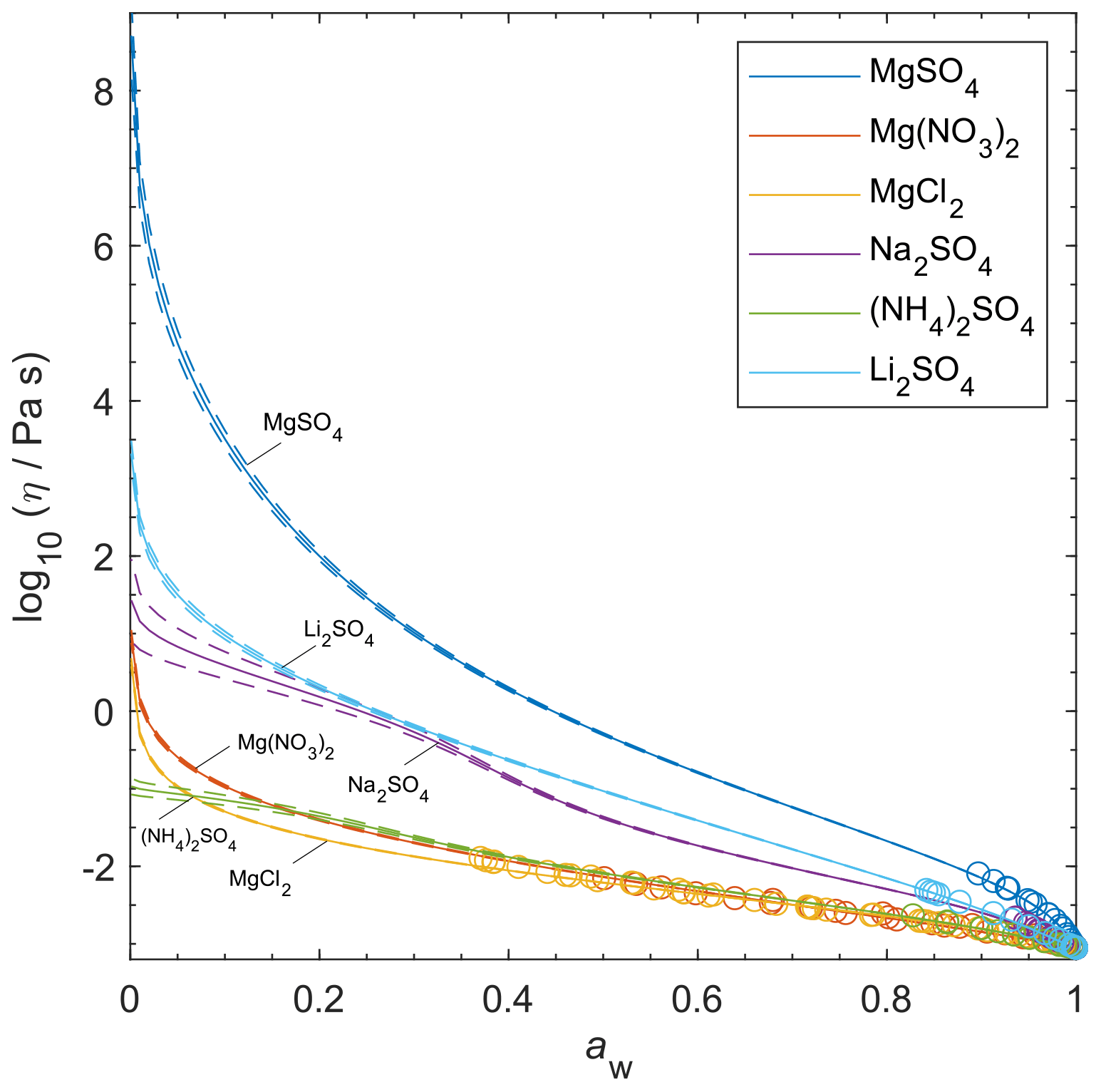
Figure 10 AIOMFAC-VISC-predicted viscosity for selected binary aqueous electrolyte solutions at 298.15 K. Model sensitivity (dashed curves) shows the impact of a ± 2 % variability in determined aerosol water content at stated water activity, a_w. Bulk measurements are shown as open circles, with colors matching the prediction curves for each electrolyte.

4.7 Comparing AIOMFAC-VISC with aqueous organic–inorganic aerosol surrogate mixtures

Room temperature measurements are available for aqueous mixtures of sucrose with Ca(NO₃)₂ and Mg(NO₃)₂ (Song et al., 2021), as well as NaNO₃ (Rovelli et al., 2019). Sucrose is commonly used as a proxy for secondary organic aerosol because it has a similar oxygen-to-carbon ratio as highly oxidized organic aerosol components and viscosity and related diffusivity data are available in the literature (Evoy et al., 2019). In Fig. 11, AIOMFAC-VISC viscosity predictions are tested for these systems at varying water activity, providing a comparison of the three organic–inorganic mixing approaches described in Sect. 3.4. Each of these mixing approaches predicts viscosities between those of the relevant sucrose-free aqueous nitrate salt solution and the aqueous (salt-free) sucrose solution (plotted in grey). As the OIR increases, the mixture viscosity prediction approaches that of aqueous sucrose, and as the OIR decreases, the prediction tends toward the viscosity of the aqueous nitrate salt. Figure 11a and b show cases for an OIR of 1, while Fig. 11c and d are for an OIR of 1.5 and 4, respectively. The reported error in viscosity for the Song et al. (2021) measurements can be as large as an order of magnitude, which is much larger than the typical reported error for bulk measurements. AIOMFAC-VISC's model sensitivity is mostly contained within the width of the error bars. Viscosity error bars for Fig. 11c and d were not available. Additional measurements are included from Richards et al. (2020b) for 1:1 (by moles) mixtures of (NH₄)₂SO₄, MgSO₄, CaCl₂, Ca(NO₃)₂, and Mg(NO₃)₂ with sorbitol, glucose, and gluconic acid. However, as the authors describe these systems in the context of gel formation – a process so far not captured by AIOMFAC-VISC – we have included these figures in the Supplement.

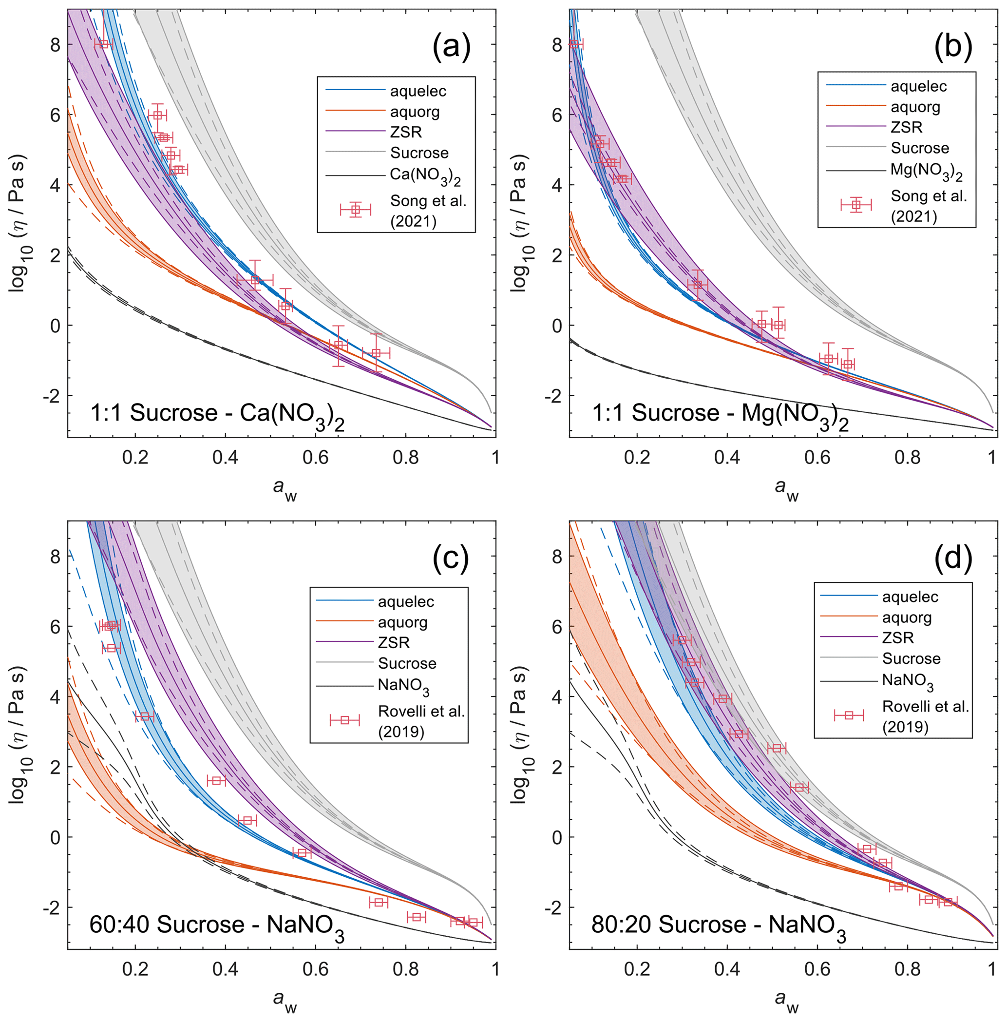
Figure 11 Viscosity predictions for aerosol surrogate mixtures containing sucrose and nitrate salts at varying water activity, a_w (RH), with a prescribed organic-to-inorganic dry mass ratio (OIR). Three mixing models – aquelec, aquorg, and ZSR – are shown alongside the viscosity measurements. Model sensitivity, defined by the impact of a ± 2 % change in aerosol water content, is shown by the dashed curves. Shaded regions show the potential viscosity prediction error introduced by a ± 5 % error in the glass transition temperature of sucrose. AIOMFAC-VISC predictions are also included for the binary aqueous sucrose and aqueous nitrate salt systems, which correspond to the organic and inorganic subsystems used in each mixing model (see Sect. 3.4).

The aquelec mixing model predictions agree best with the measurements for 1:1 sucrose–Ca(NO₃)₂ (Fig. 11a) and 60:40 sucrose–NaNO₃ (Fig. 11c), while the ZSR-style mixing rule and aquelec perform similarly for 1:1 sucrose–Mg(NO₃)₂ (Fig. 11b) and 80:20 sucrose–NaNO₃ (Fig. 11d) when uncertainties in measurements and model predictions are accounted for. In Fig. 11b, aquelec predicts values within the uncertainty of the measurements between 70 % and 30 % RH but underpredicts the measurements between 20 % and 10 % RH. The aquorg mixing model consistently predicts lower viscosity values than the other two mixing models, and this negative bias is exacerbated at low RH. The measurements for binary solutions of some salts include abrupt increases in viscosity at low RH (5 % for Ca(NO₃)₂ and 35 % for Mg(NO₃)₂, as shown in Fig. 9). This could be the result of crystallization of the salt, a glass transition, or a gel transition during the experiments. Regardless, when mixed with sucrose, this abrupt viscosity increase appears to be inhibited. Richards et al. (2020b) found that ternary organic–inorganic mixtures containing certain doubly charged cations had higher viscosity than the corresponding salt-free aqueous organic mixture, but AIOMFAC-VISC would not be able to produce such results without further additions for organic–ion effects (a potential subject of future work). Of the three systems shown here, the viscosity of aqueous sucrose is consistently higher than the ternary mixture throughout the RH range. Additional AIOMFAC-VISC predictions are shown for the mixtures from Richards et al. (2020b) in Figs. S15 and S16 in the Supplement. Richards et al. (2020a, b) hypothesized that interactions between doubly charged ions (especially cations) and certain organic compounds can lead to the formation of a gelatinous network that would have different rheological properties than a viscous liquid. Indeed, the discrepancies between the AIOMFAC-VISC predictions and these measurements may in themselves be evidence of a gel transition for these systems. Of the seven organic–inorganic mixtures shown in the Supplement figures, only a mixture of (NH₄)₂SO₄ and gluconic acid is reasonably represented by AIOMFAC-VISC, suggesting that the gel-forming ability of (NH₄)₂SO₄ is weaker than that of the other electrolytes shown. As in Fig. 11a and b, the measurement point reported for the lowest RH is given as a lower bound estimate of the viscosity, and the upper vertical error bar is unbounded. In the Supplement figures, these points are meant to indicate a discrete change in behavior from a viscous liquid to a gel.

In terms of computational speed, the ZSR mixing model takes approximately 5 to 6 times longer than aquelec or aquorg (see Tables S1 and S2 in the Supplement). In dynamic simulations that may require repeated calls to AIOMFAC, such as kinetic multilayer diffusion models, this time difference may be an important consideration.

5 Atmospheric implications

While AIOMFAC-VISC is flexibly designed to predict viscosity for bulk solution phases, in case of equilibrium gas–particle partitioning computations, it is additionally capable of calculating the viscosities of individual aerosol phases when the presence of liquid–liquid phase separation is predicted. This functionality is expected to be especially important in future research on aerosol phase state and in estimating molecular diffusion inside of aerosol particles, some of which may be multiphase particles. To illustrate the utility of AIOMFAC-VISC for atmospheric aerosol, we show how AIOMFAC-VISC can predict the viscosities of two coexisting liquid phases and compare the result to a scenario of assuming a homogeneously mixed single phase. Furthermore, we carry out predictions of the viscosities of both particle phases during the idealized adiabatic ascent of an air parcel. Finally, we show AIOMFAC-VISC-predicted particle viscosity of selected aerosols equilibrated to the thermodynamic conditions reported for an atmospheric vertical profile collected at Maniwaki, Quebec. In the context of meteorology, the effect of changing atmospheric pressure on viscosity is expected to be negligible and is therefore ignored.

Liquid–liquid phase separation (LLPS) has been observed in aerosol particles (Bertram et al., 2011; Song et al., 2012; You et al., 2014), and capturing this behavior is essential to accurately characterizing aerosol mass concentrations. Coexisting liquid phases are expected to occur when low-polarity and highly polar organics are present in a particle and/or when inorganic ions, water, and moderate-to-lower-polarity organics are present or when weakly oxidized SOA material partitions into an existing aqueous aerosol (e.g., Huang et al., 2021). Relatively fresh SOA of moderate-to-lower polarity is likely to form a second, organic-rich phase that will coexist with an aqueous ion-rich phase. By contrast, aged SOA includes organic species that are more highly oxygenated, and these species will more likely dissolve and mix with water and ions in a single liquid phase. AIOMFAC-VISC can be used to predict the viscosity of any number of condensed phases, as we have done for a mixture of α-pinene-derived SOA and ammonium sulfate with an OIR=1 exhibiting two liquid phases over a wide range in RH (Fig. 12). In the LLPS case shown in Fig. 12a, two liquid phases are predicted, and the organic-rich phase attains a semi-solid viscosity for RH<80 %. When we assume a single mixed phase (Fig. 12b), the predicted viscosity is less than that of the organic-rich phase in Fig. 12a, due to the plasticizing effect of water contributed by the hygroscopic ions. A phase-separated aerosol, with a more viscous organic-rich shell, will likely be more resistant to chemical processing than a homogeneously mixed aerosol (Zhou et al., 2019). While the viscosity of the organic-rich phase becomes semi-solid (>10² Pa s) below RH=0.8, the single mixed phase remains liquid-like (<10² Pa s) until RH=0.2. The calculations for the phase viscosities in the LLPS case were carried out in two steps: first, an AIOMFAC-based coupled gas–particle and liquid–liquid equilibrium computation was performed to determine the phase compositions while not computing the viscosities in the process (since it is unnecessary) and, second, AIOMFAC-VISC is run for the compositions of the determined phases to provide the viscosities and associated estimations of uncertainties. The surrogate mixture representing α-pinene SOA, defined in Table S4 in the Supplement, consists of compounds that span a range of polarities and miscibilities with water and electrolytes. This explains an abrupt local maximum in the predicted organic-rich phase viscosity. As a_w values approach and exceed 0.98, this is accompanied by relatively large water uptake, and the liquid–liquid partitioning of the organic compounds changes substantially. Most of the moderately water soluble organics partition to the aqueous ion-rich phase; only the least polar organics remain in the now-depleted organic-rich phase. The remaining organic-rich phase includes dimers and a smaller water content, which leads to an increase in the predicted viscosity of that phase. As even higher a_w values are reached, all compounds become miscible in a single, water-rich liquid phase, which has a viscosity close to that of pure water.

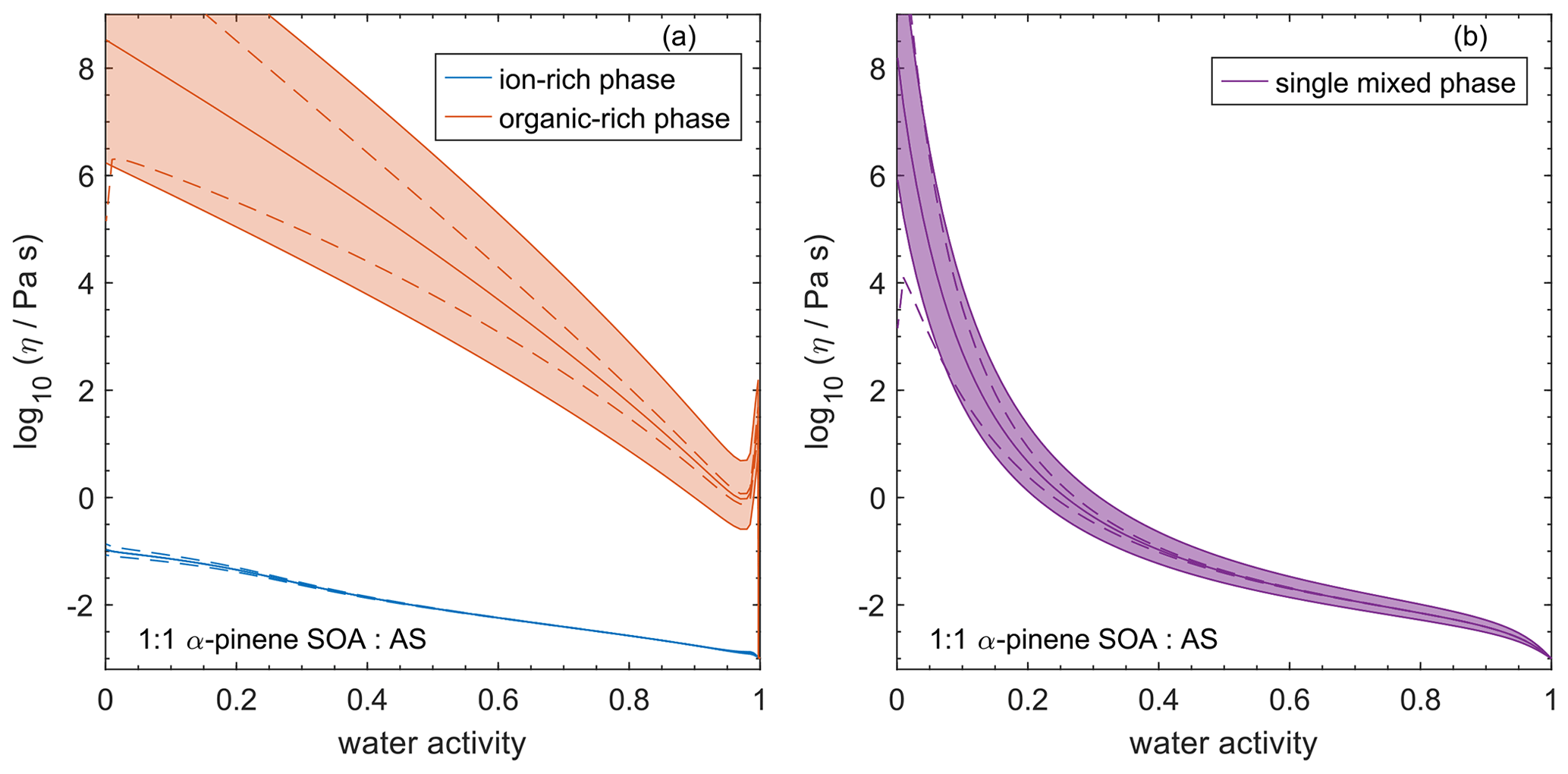
Figure 12 Viscosity predictions for aerosol surrogate mixtures containing α-pinene SOA and ammonium sulfate at varying water activity, a_w (RH), with an overall organic-to-inorganic dry mass ratio (OIR) of 1 and T=293.15 K. (a) Viscosities of the individual coexisting liquid phases predicted by AIOMFAC LLPS model; blue: inorganic ion-rich phase; orange: organic-rich phase. (b) Predictions for a forced single mixed phase. The aquelec mixing model is used to calculate the viscosities of the organic–inorganic mixtures. Model sensitivity, defined by the impact of a ± 2 % change in aerosol water mass, is shown by the dashed curves. Shaded regions show the potential viscosity prediction error introduced by a ± 5 % error in the average glass transition temperature of the individual α-pinene SOA surrogate components.

Figure 13 shows the predicted viscosities for phase-separated particles consisting of α-pinene SOA and ammonium sulfate (overall OIR of 1) as a function of temperature and RH. Given an average oxygen-to-carbon ratio of about 0.5 for α-pinene SOA, its mixture with aqueous ammonium sulfate is expected to result in nearly complete separation of the salt and SOA into distinct phases, except at RH levels exceeding 99.5 % (Bertram et al., 2011; Zuend and Seinfeld, 2012). Over the same ranges of RH and temperature, the organic-rich phase viscosity spans 18 orders of magnitude, whereas the ion-rich phase spans only 2 orders of magnitude, with liquid-like viscosities prevailing at all conditions. However, note that this composition and viscosity computation was conducted by assuming the ions to remain dissolved over the entire RH range. Depending on the initial conditions, such as starting with dry or deliquesced particles, ammonium sulfate could potentially be present in solid–liquid equilibrium with the organic-rich phase below 80 % RH. Ammonium sulfate would be expected to be predominantly in a crystalline state for $\text{RH}<\sim \mathrm{35}$ % due to efflorescence (Ciobanu et al., 2010), such that the predictions of the viscosity for lower RH levels in the ion-rich phase are hypothetical. Nevertheless, those viscosities are indicative of expected viscosity levels in similar aqueous ion-rich phases containing inorganic species that would less likely crystallize (such as certain nitrate salts).

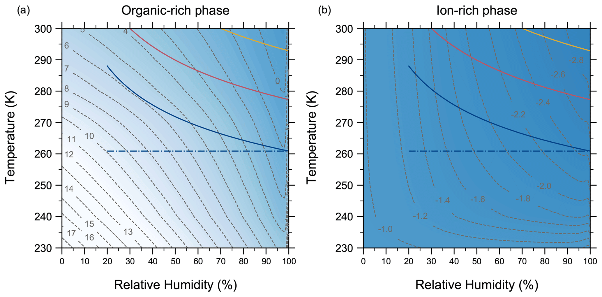
Figure 13 Viscosity predictions for coexisting phases in internally mixed aqueous α-pinene SOA + ammonium sulfate particles with an overall OIR of 1. Dashed curves are contours of ${\log }_{\mathrm{10}}(\mathit{\eta }/[\mathrm{Pa}\mathrm{s}\left]\right)$. The three solid-colored curves represent idealized adiabatic ascent of an air parcel for different initial conditions at the surface. The prescribed initial conditions are T=288 K, RH=20 % (blue); T=300 K, RH=30 % (pink); and T=300 K, RH=70 % (yellow). The dash–dotted blue horizontal line shows the range of RH that could be experienced by particles if they survive cloud processing and stay at the same height, while RH may change. The aquelec mixing model is used to calculate the viscosity of organic–inorganic mixtures.

Charnawskas et al. (2017) found that α-pinene SOA particles containing sulfate do not significantly impact ice formation in mixed phase clouds, basing their conclusion on chamber experiments and numerical diffusion modeling. According to the authors, heterogeneous ice nucleation of α-pinene SOA/sulfate particles would only occur below temperatures of approximately 222 K. Although the organic-rich phase of our α-pinene SOA/AS surrogate mixture can attain a glassy viscosity (i.e., 10¹² Pa s) at temperatures as high as 265 K (when RH=0 %), Charnawskas et al. (2017) consider that deliquescence may occur on these particles before a glassy viscosity is attained, in which case these particles would no longer be suitable for ice nucleation.

Finally, we can use AIOMFAC-VISC to predict the viscosities of these two phases at different vertical levels in the atmosphere. To provide an example, we extracted temperature and relative humidity values from two sample vertical atmospheric profiles at Maniwaki, Quebec, measured on 7 February 2020 and 1 July 2020. We calculated the viscosities of the two phases for each vertical profile assuming the particles to be in equilibrium with the measured environmental conditions (T, RH) at each altitude level. This is unlike the case of an adiabatically lifted air parcel, for which the temperature and RH may substantially differ from those of its environment. It is worth noting that as viscosity increases, diffusion of water and other species is increasingly limited, which could affect equilibration timescales during adiabatic ascent, especially at high altitudes. In Fig. 14, we show the viscosities of the organic-rich and ion-rich phases plotted up to an altitude of approximately 35 km. Examining these two profiles side by side provides useful information about the potential distribution of viscous (semi-solid) and glassy aerosol phase states in the atmosphere. As expected, the viscosity of the organic-rich phase is consistently several orders of magnitude higher than the viscosity of the aqueous ion-rich phase. The predicted viscosity for the ion-rich phase remains below 10² Pa s throughout the vertical extent of the atmosphere. While higher liquid-state viscosities are not predicted for the ion-rich phase, freezing and efflorescence are still possible – and would likely occur at the low temperatures in the upper troposphere and lower stratosphere, with associated effects on phase state.

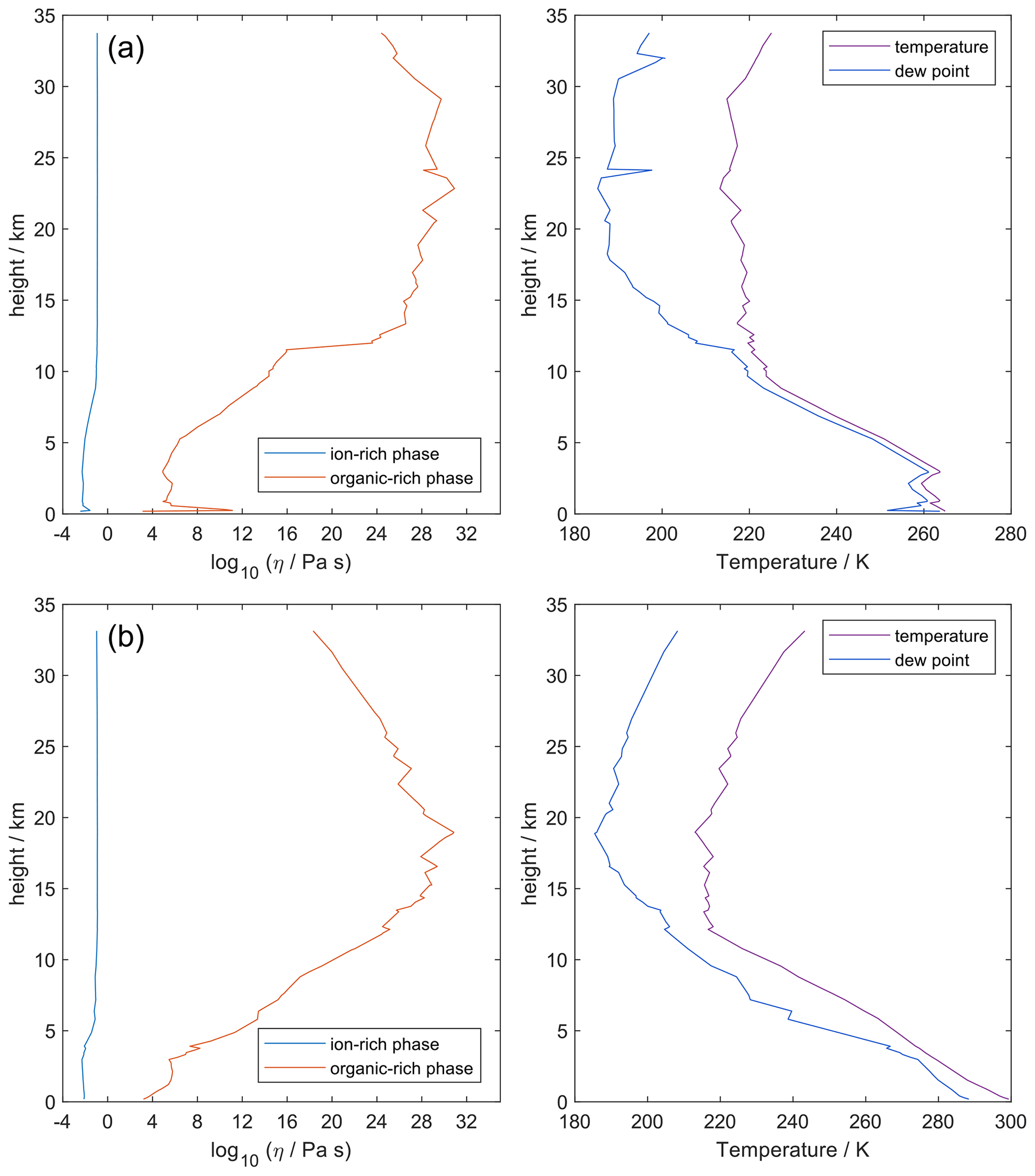
Figure 14 Viscosity predictions for observed temperature and relative humidity profiles using liquid–liquid phase separated aerosol particles containing α-pinene SOA surrogate compounds and ammonium sulfate. Relative humidity and temperature data are taken from atmospheric soundings collected at Maniwaki, Quebec (station code: WMW) for 7 February 2020 at 12:00 UTC (a) and 1 July 2020 at 00:00 UTC (b). Left panels show AIOMFAC-VISC viscosity predictions, and right panels show corresponding measurements of the air and dew point temperatures. OIR is approximately equal to 1 for warm surface conditions and increases gradually to approximately 11 for the coldest observed temperatures owing to the increased condensation of semivolatile organic compounds in this surrogate system. Sounding data are provided by the University of Wyoming (http://weather.uwyo.edu/upperair/sounding.html, last access: 4 October 2021).

The February sounding (Fig. 14a) was collected during a winter storm. A local maximum in the predicted viscosity is observed near the surface and corresponds to a local minimum in relative humidity between 200 and 300 m. There is also an abrupt change in relative humidity above 12 km, likely indicating the tropopause region. Below this altitude, there is sufficient water content in the aerosols to have a diminishing effect on the viscosity (when ignoring potential freezing and/or freeze concentration of the phase). Above this altitude, the predicted viscosity of the organic-rich phase increases by several orders of magnitude, and it is virtually certain that SOA-rich aerosol phases at this height would be glassy. However, it is important to consider assumptions made and the example character of such calculations. They provide information about the expected viscosities that equilibrated particles of similar composition would exhibit when present at different altitude levels. We do not suggest that SOA-rich aerosols are typically found in the stratosphere. Wet and dry removal processes will prevent most tropospheric aerosol particles from reaching the stratosphere (Jacobson, 2002, p. 137). The July sounding (Fig. 14b) was collected during a warm, moderately dry day without clouds, and the vertical profile for viscosity of the organic-rich phase shows a more gradual increase in viscosity with height. In this case, the lack of moisture in the planetary boundary layer means that the organic-rich phase attains a glassy viscosity at approximately 5 km altitude. The presence of glassy SOA particles at high altitudes has been previously hypothesized (Koop et al., 2011; Zobrist et al., 2008), and their utility as ice nuclei has been more recently established for isoprene-derived SOA particles (Wolf et al., 2020).

6 Conclusions

A new predictive model has been developed and parameterized to enable calculations of the viscosity of aqueous electrolyte solutions. Furthermore, the earlier framework for aqueous organic mixtures has been successfully coupled with the electrolyte model, providing a more general model applicable to aqueous organic–inorganic mixtures. The AIOMFAC-VISC electrolyte model is based on Eyring's absolute rate theory for viscous flow, which has been used previously to describe the viscosity of aqueous electrolyte solutions up to approximately 10 molal. A new expression for the molar Gibbs energy of activation for viscous flow for aqueous electrolyte solutions was introduced, defining contributions from individual ions and present cation–anion pairs. Fifty-three aqueous electrolyte systems comprising 7055 data points were used to simultaneously fit the AIOMFAC-VISC electrolyte model. AIOMFAC-VISC's ionic coefficients are fitted using viscosity measurements at a wide range of concentrations as opposed to classical B coefficients, which were fitted at dilute conditions. AIOMFAC-VISC closely fits the available data and produces smooth predictive extrapolations, performing nearly as well as Laliberté's model, which is considered a benchmark. The parameterized AIOMFAC-VISC model also aligns with more recent measurements of aerosol surrogate mixtures containing aqueous nitrate salts.

Three mixing approaches were examined; aquelec and ZSR were found to be approximately equally accurate. The aquelec mixing approach is suggested as the preferred choice for use of AIOMFAC-VISC within dynamic (kinetic) simulations of viscosity or diffusion, because it is less computationally expensive. AIOMFAC-VISC's full functionality allows predictions for aqueous organic–inorganic mixtures consisting of an arbitrary number of organic compounds and inorganic ions. For systems that undergo phase separation according to an AIOMFAC-based liquid–liquid equilibrium computation, the viscosity of each phase can be computed once the equilibrium composition has been determined. Viscosity predictions for α-pinene-derived SOA were discussed in the context of idealized adiabatic ascent of an air parcel and observations from two atmospheric soundings collected in Maniwaki, Quebec. Future experimental work on a wider range of compositions and a more diverse set of multicomponent systems (presently highly data limited) may provide data and insights that could allow further refinements of the organic–inorganic mixing model. AIOMFAC-VISC may also provide an opportunity to further explore aerosol phase state and state transitions, especially gel transitions, which have become a topic of interest in laboratory aerosol studies (Song et al., 2021; Richards et al., 2020a, b).