the Creative Commons Attribution 4.0 License.
the Creative Commons Attribution 4.0 License.
 | 09 Mar 2022
Unveiling atmospheric transport and mixing mechanisms of ice-nucleating particles over the Alps
Claudia Mignani
Mario Schär
Lucie Roth
Michael Sprenger
Jan Henneberger
Ulrike Lohmann
Cyril Brunner
Precipitation over the mid-latitudes originates mostly from the ice phase within mixed-phase clouds, signifying the importance of initial ice crystal formation. Primary ice crystals are formed on ice-nucleating particles (INPs), which measurements suggest are sparsely populated in the troposphere. INPs are emitted by a large number of ground-based sources into the atmosphere, from where they can be lifted up to cloud heights. Therefore, it is vital to understand vertical INP transport mechanisms, which are particularly complex over orographic terrain. We investigate the vertical transport and mixing mechanisms of INPs over orographic terrain during cloudy conditions by simultaneous measurements of in situ INP concentration at a high valley and a mountaintop site in the Swiss Alps in late winter 2019. On the mountaintop, the INP concentrations were, on average, lower than in the high valley. However, a diurnal cycle in INP concentrations was observed at the mountaintop, which was absent in the high valley. The median mountaintop INP concentration equilibrated to the concentration found in the high valley towards the night. We found that, in nearly 70 % of the observed cases, INP-rich air masses were orographically lifted from low elevation upstream of the measurement site. In addition, we present evidence that, over the course of the day, air masses containing high INP concentrations were advected from the Swiss plateau towards the measurement sites, contributing to the diurnal cycle of INPs. Our results suggest a local INP concentration enhancement over the Alps during cloud events.
- Article
(11151 KB) - Full-text XML
- BibTeX
- EndNote


Precipitation serves as a major source of fresh water in the global hydrological cycle. Changing distribution patterns in precipitation may increase the risk of droughts and floods (Rosenfeld et al., 2008; Chow et al., 2013) and could be associated with political conflicts (Tignino, 2010). Weather forecasts and climate change projections of precipitation remain difficult for many reasons, including the lack of available data and an understanding of relevant cloud processes (Hegerl et al., 2015). The formation of precipitation is linked to the evolution of cloud microphysical properties, which is particularly complex for mixed-phase clouds (MPCs) due to the co-occurrence of supercooled liquid droplets and ice crystals (e.g., Wegener, 1911; Pruppacher and Klett, 2010; Lohmann et al., 2016b). MPCs can exist in the temperature range between 0 ∘C and approximately −38 ∘C; thus, they are frequently observed over the Alps (e.g., Henneberger et al., 2013; Lohmann et al., 2016a; Beck et al., 2017). Atmospheric aerosol particles can alter the cloud microphysics, subsequently affecting precipitation formation and evolution (e.g., Borys et al., 2003; Rosenfeld et al., 2008; Muhlbauer and Lohmann, 2009) for which the ice phase is important (Field and Heymsfield, 2015; Mülmenstädt et al., 2015; Heymsfield et al., 2020). In the absence of external snow sources, e.g., snow sedimenting from higher cloud layers (seeder–feeder effect; see, e.g., Ramelli et al., 2021a; Lee et al., 2000, and references therein), ice crystals in MPCs are initially formed via heterogeneous ice nucleation. Heterogeneous ice nucleation is catalyzed by sparse aerosol particles, called ice-nucleating particles (INPs), which provide a surface for nucleation (see, e.g., Wegener, 1911; Vali, 1971; Pruppacher and Klett, 2010; Murray et al., 2012; Vali et al., 2015). The aerosol effect on the cloud microstructure highlights the crucial need to understand the spatiotemporal INP availability – especially the vertical transport to cloud heights. In the atmosphere, a variety of aerosol particles have been found to act as INPs, such as mineral dust particles, pollen, biological or organic compounds, and also anthropogenically created particles from, e.g., biomass burning or combustion (Kanji et al., 2017; Huang et al., 2021, and references therein). Depending on the source, these particles have a different ice nucleation temperature (Kanji et al., 2017; Huang et al., 2021, and references therein). However, the spatial abundance and distribution of INPs in the atmosphere is highly uncertain (see, e.g., Demott et al., 2010; Kanji et al., 2017; Murray et al., 2021).
Most atmospheric aerosol particles have their sources near Earth's surface and are, therefore, found within the first few kilometers above ground in the troposphere, i.e., they are confined within the planetary boundary layer (PBL). In an idealized view, any PBL is in a well-mixed state when the potential temperature, aerosol number concentrations, and total humidity (sum of specific humidity and cloud water) are constant with height (see, e.g., Stull, 1988; Chow et al., 2013). The top of a well-mixed PBL is, among other indicators, characterized by an abrupt increase in potential temperature, decrease in aerosol number concentration, and decrease in total humidity (Stull, 1988; Chow et al., 2013). In contrast to the description of a well-mixed PBL over a flat surface, an accurate description of the PBL over a complex mountainous terrain is complicated by a variety of processes, such as orographic gravity waves, moist convection, and turbulent transport (see, e.g., Rotach and Zardi, 2007; Lehner and Rotach, 2018). Whereas the transport of pollutants (aerosol particles or gas) has been previously studied (e.g., Baumann et al., 2001), less is known about the transport of INP. With the PBL being confined close to the surface, higher aerosol number concentrations can be found at the same altitude (in meters above sea level; ) over orographic terrain, compared to, for example, flatlands at sea level. This raises the question of whether an increased availability of INPs at higher altitudes in orographic regions is a common feature.
Conen et al. (2017) reported an altitudinal gradient of daily averaged concentrations of INPs active at −8 ∘C, based on parallel measurements done between May and September at three sites of different altitudes located in Switzerland, and found a decrease of roughly 50 % with each kilometer in altitude. Poltera et al. (2017) found that, near the High-Altitude Research Station Jungfraujoch (3580 ), the vertical extent of the PBL can be increased by convection over the course of a day. Lacher et al. (2018) observed that INP concentrations around −31 ∘C are elevated during times of boundary layer intrusions at Jungfraujoch, suggesting that INPs are also more numerous within the PBL aerosol. Relating INP concentration as an aerosol subset to the ambient aerosol concentration is highly dependent on the air mass and precipitation history (Mignani et al., 2021), as aerosol particles and INPs follow different accumulation and depletion mechanisms. Any aerosol particle can potentially be removed by dry deposition or impaction scavenging. Additionally, aerosol particles can be removed by nucleation scavenging if embedded in hydrometeors after serving as INP or cloud condensation nuclei (Lohmann et al., 2016b). Furthermore, INPs can be added due to resuspension during and after rainfall (e.g., Huffman et al., 2013; Seifried et al., 2021). The INP concentration within a plume of freshly emitted mineral dust aerosol can be deduced from the aerosol properties (using parameterizations like Niemand et al., 2012; Demott et al., 2015). Upon precipitation formation, relations between INPs and aerosol particles may be altered (Mignani et al., 2021), as the sources and sinks of INPs and aerosol particles are disproportional to each other. Thus, transport mechanisms to higher altitudes that replenish the INP concentration after cloud formation are one crucial aspect that we study here to understand the variations in INP concentration. Among many other overviews, Chow et al. (2013) and Wekker and Kossmann (2015) summarized a vast variety of wind systems in orographic terrain. Winds can increase the PBL height, which would otherwise be confined to the valley, due to the induced vertical motion of the valley atmosphere. A specific wind system can be seen as a superposition of three drivers, namely (i) the synoptic wind speed and direction, (ii) the diurnal (thermally driven) mountain–valley breeze, and (iii) the vertical stability of the air masses within the valley. Combining the three drivers to varying degrees and considering an elongated valley, three generalized wind systems are imaginable. First, the synoptic flow arriving at the orographic barrier pushes the air masses near the surface towards the mountain ridges and tops (orographic lifting as a result of advection). In the absence of upslope winds, and given the weak stratification of the air masses leeward of the ridge, the air masses will be pushed further down the leeward valley. This synoptic forcing can result in a similar effect to the diurnal warming of the slopes, yet it is a consequence of the flow being deflected by the mountain topography (Chow et al., 2013). Second, especially on sunny days, air close to the ground of slopes on the sun-exposed side of a valley heats up faster than the surrounding air, causing an upslope wind that is confined to a few hundred meters above the slopes. This situation reverts overnight when the slopes cool down, creating a downslope wind (Schmidli and Rotunno, 2010; Wekker and Kossmann, 2015). It is required that the vertical stability allows for the vertical movement of air masses and that the synoptic wind is not too strong, thereby deflecting or fully eliminating the slope winds (Barry and Chorley, 2003). This wind system is prominent during summertime and weaker in wintertime, as the snow cover on slopes causes downslope winds due to the cooling of air masses (katabatic winds) counteracting the upslope wind. Mott et al. (2015) found that an increasing fraction of snow-covered slope area resulted in stronger katabatic winds. This effect could reduce the strength of daytime upslope winds in winter. A third option is created by the mesoscale wind flowing over the orographic barrier. If the wind direction is perpendicular to the valley axis, and its speed is strong enough, it could cause large-scale eddies, mixing the atmosphere within the valley (rotors; see Chow et al., 2013, chap. 3.3).
In this study, we investigate how the distribution of INPs between a mountain and a valley site in the Alps changes spatiotemporally and discuss the underlying transport mechanisms. Whereas in situ INP concentrations were often reported either in flat regions (e.g., Mason et al., 2016; Chen et al., 2018; Ladino et al., 2019; Paramonov et al., 2020) or at mountaintops (e.g., DeMott et al., 2003; Richardson et al., 2007; Klein et al., 2010; Stopelli et al., 2014; Conen et al., 2015; Boose et al., 2016a, b; Lacher et al., 2017; Creamean et al., 2019; David et al., 2019; Mignani et al., 2021; Brunner and Kanji, 2021), we observed in situ INP concentrations simultaneously on a mountaintop and a nearby valley site (1060 m height difference; 3.65 km horizontal distance) in a complex terrain. Measurements were conducted over 8 weeks at a high sampling frequency during cloud events (for 20 min every 1.5 h) in late winter 2019 (February and March). This allowed us to draw conclusions about the vertical distribution and mixing based on two extensive datasets of INP concentrations at both sites. We analyzed the distribution of INPs at temperatures above −20 ∘C, which is relevant for MPCs. We present the difference in INP concentration between both sites and show evidence of a diurnal cycle in INP concentrations measured on the mountaintop. Based on the local topography, we describe how dynamic transport processes can enhance the INP concentration at the mountaintop site.
During the RACLETS (Role of Aerosols and CLouds Enhanced by Topography on Snow) campaign in the region of Davos, Switzerland, in February and March 2019, a complementary set of aerosol, cloud, precipitation, and snow measurements was collected (Envidat, 2019; Walter et al., 2020; Mignani et al., 2021; Ramelli et al., 2021b, a; Lauber et al., 2021; Georgakaki et al., 2021). There are two similarly equipped aerosol measurement sites, with one located on a saddle at the entrance of a high valley (Wolfgangpass; 1631 ; hereafter referred to as WOP) and the other on a mountaintop (Weissfluhjoch; 2693 ; hereafter referred to as WFJ), which are shown in Fig. 1.
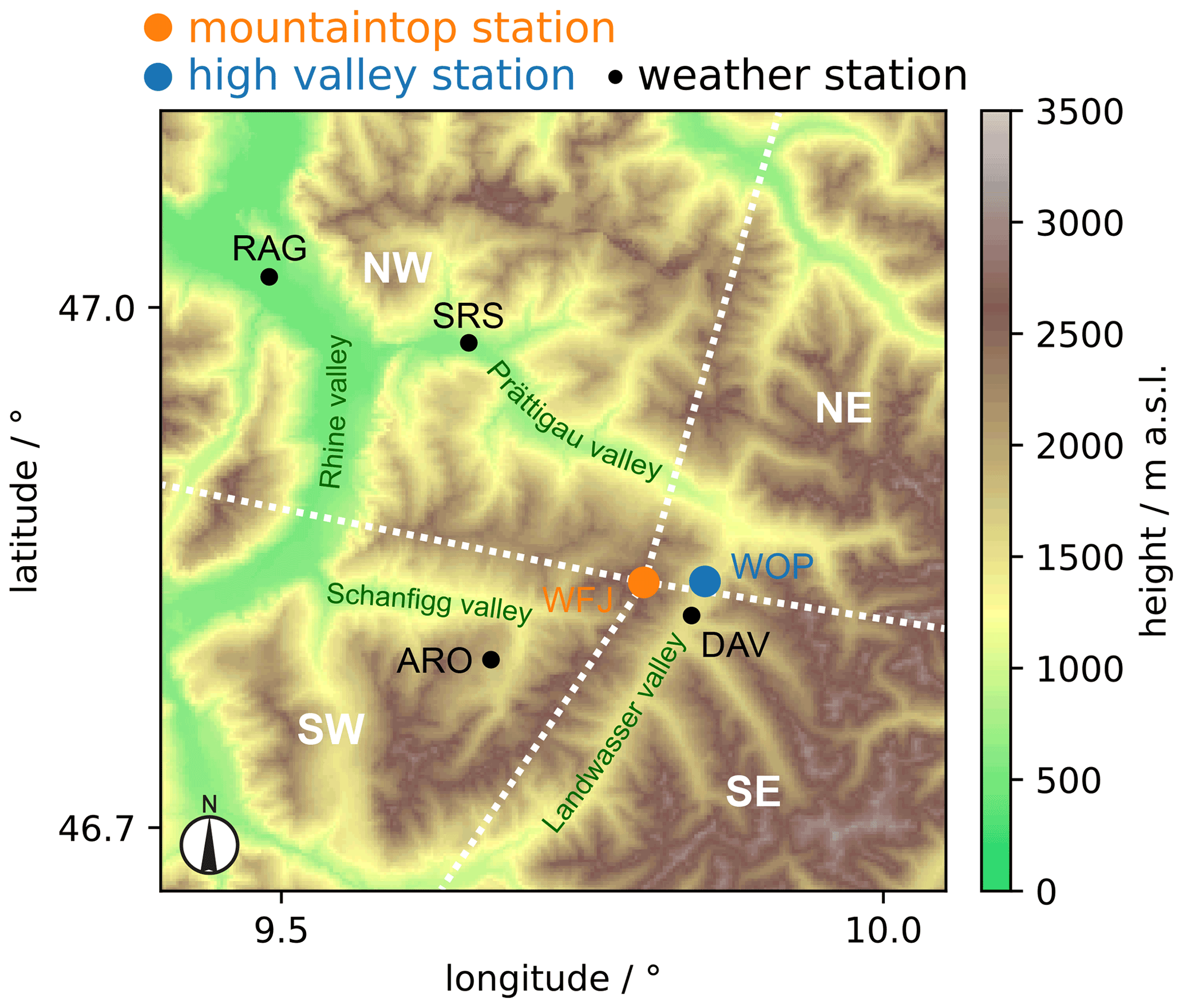
Figure 1Locations of the measurement sites. The main aerosol measurements were located at Wolfgangpass (blue; WOP; 1631 ) and Weissfluhjoch (orange; WFJ; 2693 ). The horizontal distance between WOP and WFJ measures 3.65 km. Meteorological data were retrieved from measurement stations in Arosa (ARO; 1880 ), Bad Ragaz (RAG; 498 ), Davos Dorf (DAV; 1598 ), Schiers (SRS; 628 ), and at Weissfluhjoch (WFJ; 2693 ). The white dashed lines indicate the edges of the four mesoscale wind direction sectors (NW, NE, SW, and SE) used for the analysis based on the topography used in Sect. 3.3–3.5. The topography was extracted from the digital height model DHM200 from the Federal Office of Topography, swisstopo.
2.1 Aerosol and INP measurements
Ambient aerosol was sampled through a heated total inlet at both WFJ and WOP and analyzed for properties including size and ice nucleation activity. At WOP, the inlet was mounted on a measurement trailer and consisted of a 1.5 m long vertical pipe (25 mm diameter) and a matching 0.5 m long 90∘ bend (Fig. 2a and b). At WFJ, the inlet, with a diameter of 50 mm, consisted of a 2.5 m vertical pipe and a 4.5 m long inclined pipe (height loss of approx. 0.8 m across total length; see Fig. 2c and d). Similar to Weingartner et al. (1999), both inlets were capped with a hat to prevent snow and, while sampling, particles with a diameter smaller 40 µm from entering the inlet for wind speeds of up to 20 m s−1. All outside parts (including the hat; at WOP, approx. the first 0.7 m; at WFJ, all parts) were heated to 46 ∘C to avoid riming on the outside parts, to sublimate ice crystals, and to evaporate activated cloud droplets. The evaporation of volatile compounds of the aerosol cannot be excluded. However, the relevant ice active particles in the investigated temperature regime ( ∘C) are mostly biological, which should only degrade at temperatures higher than 46 ∘C (Kanji et al., 2017; Huang et al., 2021). In addition, the flow rate through the inlet is high (300 L min−1); as such, the aerosol flow was likely at temperatures below 46 ∘C at which INPs typically do not become inactive. Contributions of resuspended particles from the snow-covered surface around the measurement sites cannot be fully excluded but are unlikely to have added significantly to the sampled aerosol due to the inlet's design (Mignani et al., 2021).
Downstream of the inlet, a custom-made flow splitter was mounted, followed by a three-way ball valve (model 120VKD025-L; Pfeiffer Vacuum GmbH, Germany) connecting a blower (model U71HL; Micronel AG, Switzerland) and a high flow-rate impinger (Coriolis® µ; Bertin Instruments, France), both operating at 300 L min−1 (see Fig. 2b for WOP and Fig. 2c for WFJ). The impinger collected particles larger than 0.5 µm (collection efficiency of 50 %, 80 %, and 94 % for 0.5, 2, and 5 µm particles, respectively; personal communication with manufacturer, 3 July 2020). During times when the impinger was idle, the ball valve was switched to the blower to create a make-up flow, thereby guaranteeing a constant flow through the inlet at all times. From the splitter, smaller connections with diameters of approximately 5 mm branched off at a 45∘ angle around the center axis. At the lowest sampling line, a commercial aerodynamic particle sizer spectrometer (APS; model 3321; TSI Incorporated, USA) recorded size distributions continuously (see Fig. 2e). Aerodynamic diameter was converted to physical diameter using a shape factor χ=1.2 and an assumed particle density ρ=2 g cm−3 (Thomas and Charvet, 2017).

Figure 2Aerosol measurement setups at WOP and WFJ. The aerosol trailer at WOP (a), with the heated inlet on the roof (blue arrow), the setup inside the aerosol trailer (b), the setup at WFJ (c), with the inlet pipe indicated (blue arrow), and the inlet mounted on a railing at WFJ (d). The schematic (e) depicts the flow connections used at both sites.
Using the aerosol-to-liquid impingers, air samples were collected for the analysis of ambient INP concentrations at both sites (as also already described for WFJ in Mignani et al., 2021). The standard protocol consisted of sampling air for 20 min (corresponding to 6 m3 of air) in 15 mL of ultrapure water (W4502-1L; Sigma-Aldrich, USA). To compensate for evaporative during the operation of the impinger, the sample liquid was refilled to 15 mL after 10 and 20 min. The sampling was directly followed by analysis for INP concentration on site, using the drop-freezing instrument DRINCZ (David et al., 2019) at WOP and LINDA (Stopelli et al., 2014) at WFJ (Mignani et al., 2021). For both instruments, sample liquid was pipetted out into small aliquots (96×50 µL for DRINCZ; 52×100 µL for LINDA) and cooled down in a cryostat until all aliquots froze. While cooling, pictures of the droplet arrays were obtained with a digital camera mounted above the droplet assay (every 15 and 5 s for DRINCZ and LINDA, respectively) to detect freezing of individual aliquots with respect to temperature in the post-processing. Cumulative INP concentrations at integer temperatures T were determined according to Vali (1971, 2019) as follows:
where FF(T) is the fraction of frozen wells at temperature T, and Va is the volume of an individual aliquot. C is a normalization factor in order to calculate the INP concentration per standard liter of sampled air (StdL−1) and is defined as follows:
with FCoriolis being the impinger flow rate (300 L min−1), tsample the sampling time (20 min), VCoriolis the sample volume after sampling (15 mL), and pambient and Tambient the mean ambient pressure and temperature during sampling, using the reference of a standard liter with pref=1013.25 hPa and Tref=273.15 K. INP concentrations have been corrected for the background of the blank ultrapure water, as described in David et al. (2019). In rare cases of very active samples (i.e., all droplets already froze above −10 ∘C), dilutions of the sample were prepared and analyzed. In this study, one value for INP concentration per temperature and sample was desired; therefore, samples and their dilutions were combined by using the number of droplets freezing at each temperature step as proportional weights. For a sample a and its dilution b, the combined INP concentration nINP,comb(T) at temperature T was calculated as follows:
where are the number of frozen droplets for sample a and b, respectively, at temperature m, are the differential INP concentrations for sample a and b, respectively, at temperature m, and ΔT is the temperature bin size (definitions of the variables analogous to Vali, 2019).
In this study, we will compare the INP concentrations measured at the two aerosol measurement sites. To ensure the comparability of both instruments, a comparison study was conducted. The results from an ambient aerosol sample collected with the impinger used in this study and analyzed with DRINCZ and LINDA are published in Miller et al. (2021, Fig. 4b). We found agreement within a factor of 2 for temperatures below −8 ∘C and within a factor of 5 above −8 ∘C, with LINDA reporting the higher INP concentrations in both temperature regimes. The observed larger deviation at warmer temperatures is not necessarily only attributed to instrumental differences but also to the large uncertainty arising from the sparsity of INPs with increasing temperatures.
2.1.1 INP measurement strategy and data selection
The RACLETS campaign aimed to better understand MPCs and their precipitation formation over the Alps. To this end, the sampling of ambient air for consequent INP analysis was targeted during cloud events and was synchronized for most samples between the two sites (WFJ and WOP). The first sample was taken around 2 h before and the last 2 h after the presence of a cloud over the sampling region. Within this time frame, samples were taken at 1.5–2 h intervals. The analysis focuses on the diurnal cycle of INP concentrations at both sites and categorizes the samples into three periods of the day (i.e., morning – 03:00–11:59 UTC; afternoon – 12:00–17:59 UTC; night – 18:00–02:59 UTC). Initially, a categorization of four periods (every 6 h) was intended, but as there were only five samples at WFJ and two samples at WOP available between 00:00–05:59 UTC, this period was split and joined with the adjacent ones. To investigate the diurnal variation in INP concentration, only sequences of samples were considered when there was at least one sample in three consecutive periods. Samples reported by Mignani et al. (2021) taken at WFJ during a Saharan dust event are excluded from this study to avoid bias from one dominating aerosol type. Applying these criteria to the datasets resulted in 111 samples obtained at both WOP and WFJ (out of a total number of samples of 157 and 155 at WOP and WFJ, respectively).
2.2 Meteorological measurements
Meteorological information in Arosa (ARO, 1880 ), Bad Ragaz (RAG, 498 ), Davos Dorf (DAV, 1598 ), Schiers (SRS, 628 ), and at WFJ (2693 ), were retrieved from the corresponding observation stations of the Swiss national weather service, MeteoSchweiz (see Fig. 1). During the campaign, a weather station installed at WOP monitored the ambient pressure, relative humidity, and temperature. Because the wind speed and direction was not measured at WOP, wind data from the nearest MeteoSchweiz observation station in Davos were used, assuming the data to be representative for WOP (in accordance with Georgakaki et al., 2021). The WFJ wind direction was found to agree with the mesoscale wind direction over Davos. Thus, references to the mesoscale wind direction in this study are based on the wind measurements at WFJ.
2.3 Back-trajectories
For every full hour of the day, kinematic back-trajectories were calculated for both sites using the Lagrangian analysis tool, LAGRANTO (Sprenger and Wernli, 2015; Wernli and Davies, 1997), each extending 5 d back in time at 10 min resolution. The back-trajectories started over the Swiss Alps, i.e., a region with complex topography, and, therefore, could only be reliably calculated if the 3D wind fields were available at a sufficient temporal and spatial resolution. To achieve this, we relied on the operational analysis of MeteoSchweiz that builds on the non-hydrostatic COSMO (Consortium for Small-scale Modeling; Baldauf et al., 2011; Schättler et al., 2015) model, with hourly wind fields at a 1 km horizontal resolution. When a trajectory left the COSMO domain (longitude 0.3–17.0∘; latitude 42.6–50.3∘), the calculation continued with the (coarser) wind fields of the ECMWF operational analysis, at a 6 h temporal resolution and interpolated to a latitude/longitude grid. Using the back-trajectories, aerosol footprint maps were generated for the two sites. The temporally closest trajectory to each INP sample was selected, and every geographic location (longitude and latitude) was noted for which the trajectory was less than 500 m above ground, indicating a potential aerosol source from these locations. Based on this criterion, many locations near mountaintops over the Alps with heights above 2500 were also indicated as sources. As these locations are considered snow covered in wintertime and, thus, feature no substantial sources of aerosol and INP, locations above the arbitrarily chosen surface height 2500 were omitted.
3.1 Overview of INP concentrations at WFJ (mountaintop) and WOP (high valley)
The distribution of INPs as a function of temperature of all samples is presented in Fig. 3. We found that, across the temperature spectrum, median INP concentrations at WOP were approximately 3 times higher than at WFJ. This supports the hypothesis of INP concentrations being generally lower at higher altitudes. Conen et al. (2017) reported INP concentrations at −8 ∘C on Jungfraujoch (3580 ) being approximately 4 times lower than at Chaumont (1136 ). Based on their results, the INP concentration at −8 ∘C at WFJ is expected to be a factor of roughly 2 lower than at WOP. During our campaign, we observed the median INP concentration at −8 ∘C to decrease by a factor of 2.4 from WOP to WFJ. Since WOP is located in a high valley and not on a mountain range as Chaumont, a higher decrease is reasonable as aerosol accumulates in the valley. Moreover, the interquartile ranges of the INP concentrations at WFJ are larger than at WOP throughout the temperature spectrum, representing a larger variability of INP at WFJ (Fig. 3). We attribute the observed larger variability at WFJ to the fact that a given perturbation in the INP number concentrations leads to a larger relative variability at lower median INP concentrations than at higher median INP concentrations. This suggests that WFJ is more susceptible to aerosol perturbations. For WFJ being located in a ski resort, local aerosol sources, such as cooking in restaurants, smoking tourists, and the preparation of the slopes at night (soot emissions from snow cats) are possible. Generally, small particles from combustion processes can be excluded due to the impinger's 50 % collection cutoff size of 0.5 µm. In addition, for the investigated temperatures and freezing mode (immersion), the contributions of local point soot emissions to ice nucleation should be negligible (Kanji et al., 2020; Vergara-Temprado et al., 2018; Mahrt et al., 2018; Chou et al., 2013). Furthermore, INP concentrations were not influenced during susceptible periods, e.g., for wind directions from the nearby kitchen to the sampling site (distance ∼ 100 m) during 10:00–13:00 LT (local time; see Fig. A1). Hence, fluctuations in the INP concentration at WFJ are expected to be caused by advected aerosol particles from the surrounding valleys or by long-range transported aerosol. This raises the question of whether there are times when the INP concentration at WFJ reaches (or even exceeds) the INPs concentration at WOP. Subsequently, we investigate the diurnal concentrations of INP at both sites in the following section.
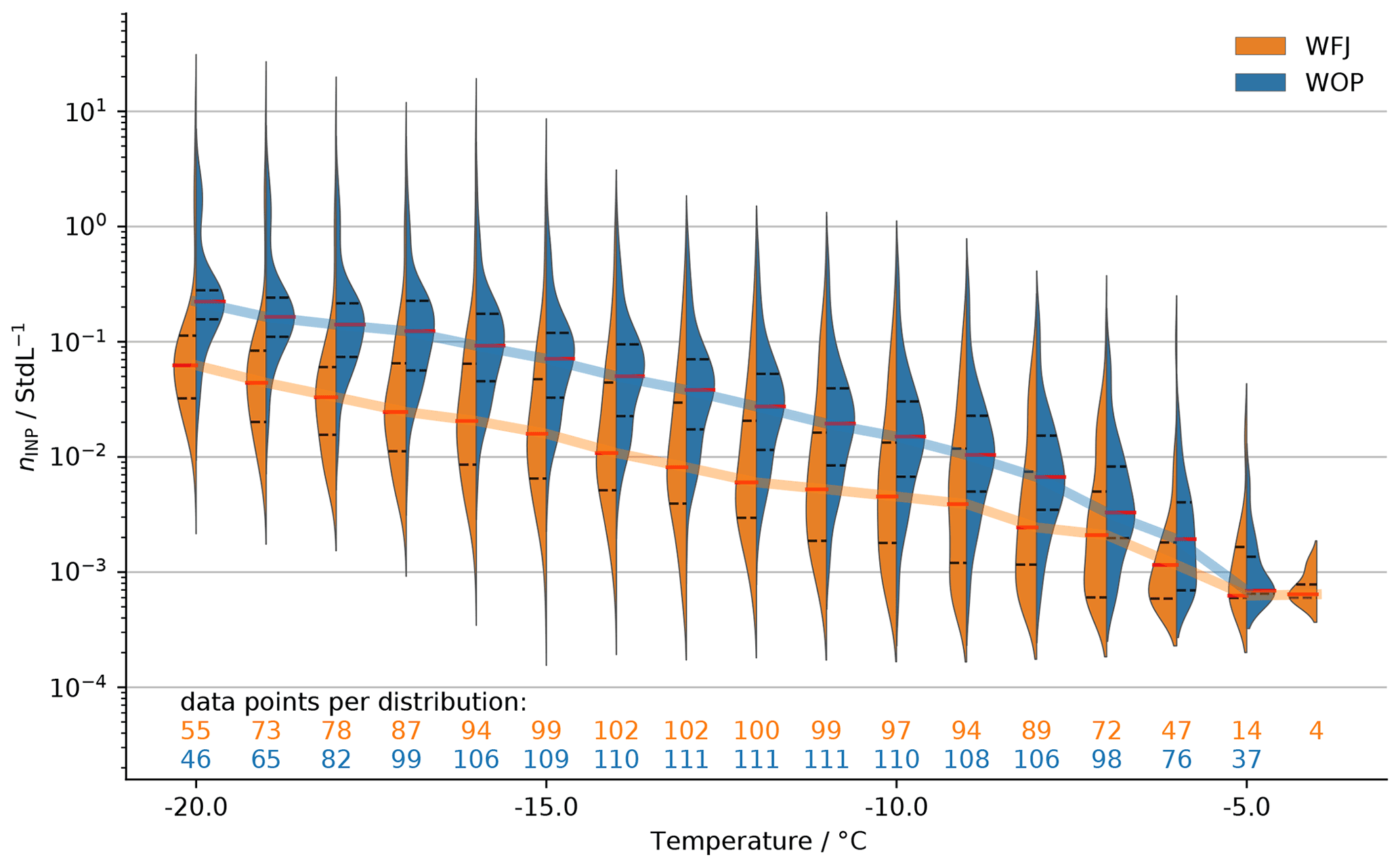
Figure 3Cumulative INP concentration (nINP) violin plots per temperature of all collected samples at WFJ (orange) and WOP (blue). For each distribution, the median is given in solid red lines, and the 25th and 75th percentiles are shown in dashed black lines. The lines connect the distribution medians. At the bottom of the figure, the number of data points at each temperature is shown in orange and blue for WFJ and WOP, respectively.
3.2 Diurnal cycle of INP concentrations
Over orographic terrain, region-specific wind systems (e.g., mountain–valley breeze) can occur in diurnal cycles (see, e.g., Nyeki et al., 2000; Chow et al., 2013; Wekker and Kossmann, 2015). A common observation is the increase in the PBL height over the day and its decrease during the night (e.g., Wekker and Kossmann, 2015; Poltera et al., 2017), which also redistributes the aerosols. To investigate the presence of a diurnal cycle in the INP concentration, samples taken at WOP and WFJ are categorized into morning, afternoon, and night (see Sect. 2.1.1).
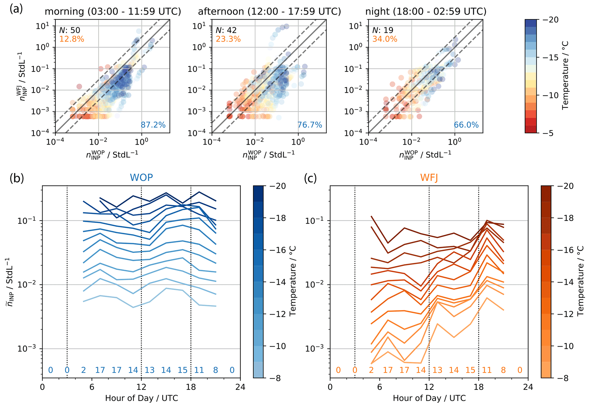
Figure 4(a) Scatterplots of INP samples taken in parallel on the mountaintop (WFJ) and high valley (WOP) site in the morning, afternoon, and at night. Samples were considered to be in parallel when their sample time differed by less than 30 min. The color indicates the activation temperature of a given pair of INP concentrations. The solid line represents the 1:1 line, whereas the dashed lines indicate an offset by a factor of 3. The number of available samples (N) per period is indicated on the upper left. The percentage of observed INP concentrations at WFJ exceeding INP concentrations found at WOP and vice versa are given in the upper left and lower right, respectively. (b, c) Time series of median INP concentration at different temperatures (from −8 to −20 ∘C in steps of 1 K) for samples taken at WOP (b) and WFJ (c). The samples were binned in 2 h intervals for the median calculations. The number of samples available within each 2 h bin is indicated at the bottom of the plot. The dotted vertical lines represent the separation times used for data selection and to calculate median values across INP spectra (see Fig. 5).
In Fig. 4a, INP concentrations at WOP against INP concentrations measured in parallel at WFJ are compared. A diurnal pattern is visible across all measurements. In the morning, nearly 90 % of the observed INP concentrations at WOP are higher than at WFJ at all temperatures. Over the course of the day, the INP concentrations at WFJ progressively increase, reaching similar levels to WOP during the night. To investigate this observed diurnal pattern in detail, we present the median INP concentration between −8 and −20 ∘C, binned per 2 h, as a function of the time of day in Fig. 4b and c. While the median INP concentrations at WOP do not exhibit a large variation over the course of a day, median INP concentrations at WFJ are lowest around 11:00 UTC and increase by nearly 1 order of magnitude until 19:00 UTC. The increase is less pronounced in INP concentrations active at temperatures colder than −15 ∘C. This could be explained by a paucity in the data for colder temperatures, where active samples were not included in the analysis, as all their droplets were already frozen above −15 ∘C. This is shown by a decrease in the number of data points (see Fig. 3) towards colder temperatures.
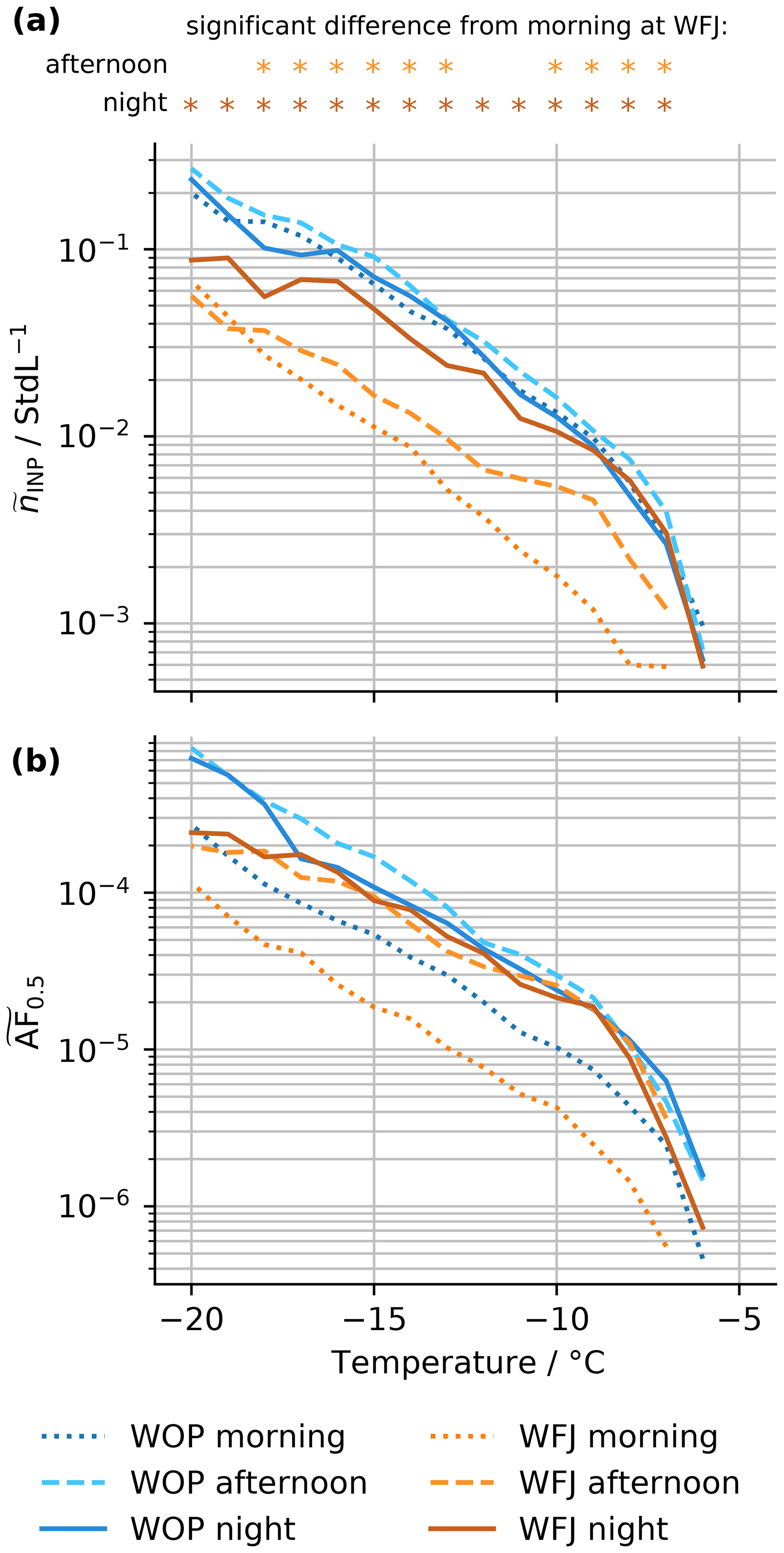
Figure 5Median (cumulative) INP concentrations (a) and median activated fractions (b) for the mountaintop (WFJ; orange) and high valley (WOP; blue) sites for the three time periods of the day. The morning period (03:00–11:59 UTC; in dots), afternoon period (12:00–17:59; dashed), and night period (18:00–02:59 UTC; solid) are shown (see dotted lines in Fig. 4b and c). Above panel (a), asterisks indicate if the median INP concentration at WFJ in the afternoon and night, respectively, is significantly (significance level p<0.05) different from in the morning based on a Mann–Whitney U test per temperature.
In Fig. 5a and b, the median INP concentration and the median activated fraction (AF0.5, ratio of INP concentration and total aerosol concentration of particles with diameter larger 0.5 µm), respectively, are shown as a function of temperature for the three time periods (morning, afternoon, and night). The significance of the differences in the medians at WFJ in the morning compared to in the afternoon and night, respectively, was determined using the Mann–Whitney U test (significance level p<0.05) per temperature. As there is a significant increase in median AF0.5 at WOP from the morning to the afternoon, whereas the corresponding median INP concentration remains almost identical, the median aerosol number concentration must have decreased (see Fig. A2). Regarding the sources of the aerosol particles at WOP during the night (i.e., between 00:00 and 06:00 UTC) there are two likely pathways potentially occurring simultaneously with varying magnitude, i.e., ice-nucleation-inactive aerosol could (i) have been brought down with air masses from higher altitude (if INPs have been previously removed by solid precipitation) due to the nocturnal stratification of the atmosphere or (ii) be emitted by local sources in the valley. For the latter, two potential sources are imaginable. First, soot emissions from traffic could be confined to the valley floor by a nighttime inversion layer. Fresh soot is not expected to contribute to the observed INP concentrations and, thus, reduce the AF0.5 (following the same argumentation as in Sect. 3.1). Second, aerosol from biomass burning from the heating of neighboring houses could also be confined in the valley. From the study of McCluskey et al. (2014), the expected median AF0.5 associated with different biomass burning events ranges between 10−5 and 10−4 for temperatures of −15 and −20 ∘C, respectively. Consequently, biomass burning emissions containing hardly any INP would dilute the INP concentration within the total aerosol population and, thus, decrease the AF0.5 at WOP. All three scenarios (sedimentation of aerosol from aloft, confined ground emissions from traffic, and heating emissions) could explain the lower AF0.5 at WOP during the morning period but remain speculative. The decrease in median AF0.5 from the afternoon to the night at WOP is comparable to the decrease observed in median INP concentrations, indicating either an increase in ice-nucleation-inactive aerosol at WOP or the depletion of INPs. At WFJ, the median AF0.5 (significantly) proportionally increases more than the median INP concentrations from the morning to the afternoon, suggesting an increase in INPs or a decrease in ice-nucleation-inactive aerosol. Towards the night, the median AF0.5 at WFJ remains at a similar level to that in the afternoon, while the median INP concentrations significantly increased further. As local INP sources at WFJ are unlikely (see Sect. 3.1); the diurnal trend at WFJ indicates that air masses of the same AF0.5 are likely to have mixed with the air masses at WFJ or replaced the air masses of lower INP and aerosol concentration at WFJ. Whether these air masses originated from the valley and were transported to WFJ or if WFJ and WOP are affected by the same air masses is not clear yet. The disproportional changes in median INP concentration and AF0.5 at both sites likely caused by the aforementioned effects also imply the absence of a relation between the INP concentration and aerosol number concentration. A more detailed analysis confirmed that a stable relation between the two variables is not present in the dataset (Appendix A3).
WFJ is susceptible to external perturbation (Sect. 3.1), and since the increase in INPs during the afternoon occurs on a daily basis, it is conceivable that it is caused by local or regional conditions rather than global long-range transport (which is excluded based on the sample selection; see Sect. 2.1.1). A possible explanation would be a local or regional wind system by which INPs are transported from lower altitude towards the mountaintop. That the valley serves as supply for INPs at higher altitude or is affected by the same air masses is supported by the equilibration of INP concentrations and activated fractions at both sites during the night.
3.3 Overview of the local topography and valley winds
In this section, potential transport mechanisms over the orographic terrain are considered. For the subsequent analysis, we divided the data into four mesoscale wind direction sectors (see Fig. 1), each featuring a distinct topography. Towards the south and the west, the mountain ridges branching off WFJ were used as topographic divisions. For north and east, division lines were set orthogonal to the valley axes. Towards the northwest (NW), the Prättigau valley stretches down to the Rhine valley (approx. 500 ; see Fig. 1). During the NW wind, the channeled winds in the valley could transport aerosol and, thus, INPs from the Rhine valley towards WFJ and WOP (Fig. 6a). From the southwest (SW), the topography also features a valley stretching down to the Rhine valley (Fig. 6c). Different to the NW case, the Schanfigg valley only connects directly to WFJ, while WOP is located leeward of WFJ. Thus, during SW wind, it is conceivable that we did not always observe the same air masses at WFJ and WOP. Same air masses are only observed if the air in the Landwasser valley is weakly stratified, such that the air masses arriving at WFJ from the Schanfigg valley would follow the leeward slope down to WOP. The topography from southeast (SE) is more complex and the valley wind direction is sensitive to even small deviations in mesoscale wind direction (Fig. 6d). When the wind direction is from the SE, near-surface winds are channeled within the valleys in mesoscale flow direction. At the end, valley air masses would be deflected towards WOP by the mountain barrier around WFJ. Due to the inertia of the air masses, they could reach WFJ if the wind speed is high enough and the stability of the air mass is favorable (i.e., the absence of a stable air mass layer potentially preventing rising air masses). If the wind direction is more southerly, however, near-surface winds would follow the Landwasser valley (see Fig. 1), reaching WOP but not necessarily WFJ. Last, the topography northeast (NE) of WFJ does not channel the flow upstream of WFJ as NE wind first passes over high mountain ridges and then crosses the junction of the Prättigau and Landwasser valleys (Fig. 6b). A north wind in the Landwasser valley will be induced, but aerosol transport to WFJ might only be possible if the lower air masses are conditional and unstably layered. The Prättigau and Schanfigg valleys (see Fig. 1) have the potential to act as ramps introducing INP-rich aerosol from lower elevations to higher altitudes in the case of NW and SW mesoscale wind, respectively (Fig. 6a and c). In the next section, we further investigate this mechanism by utilizing the Froude number, which can be used as a proxy for whether a low-level air mass is able to pass over mountain barriers.
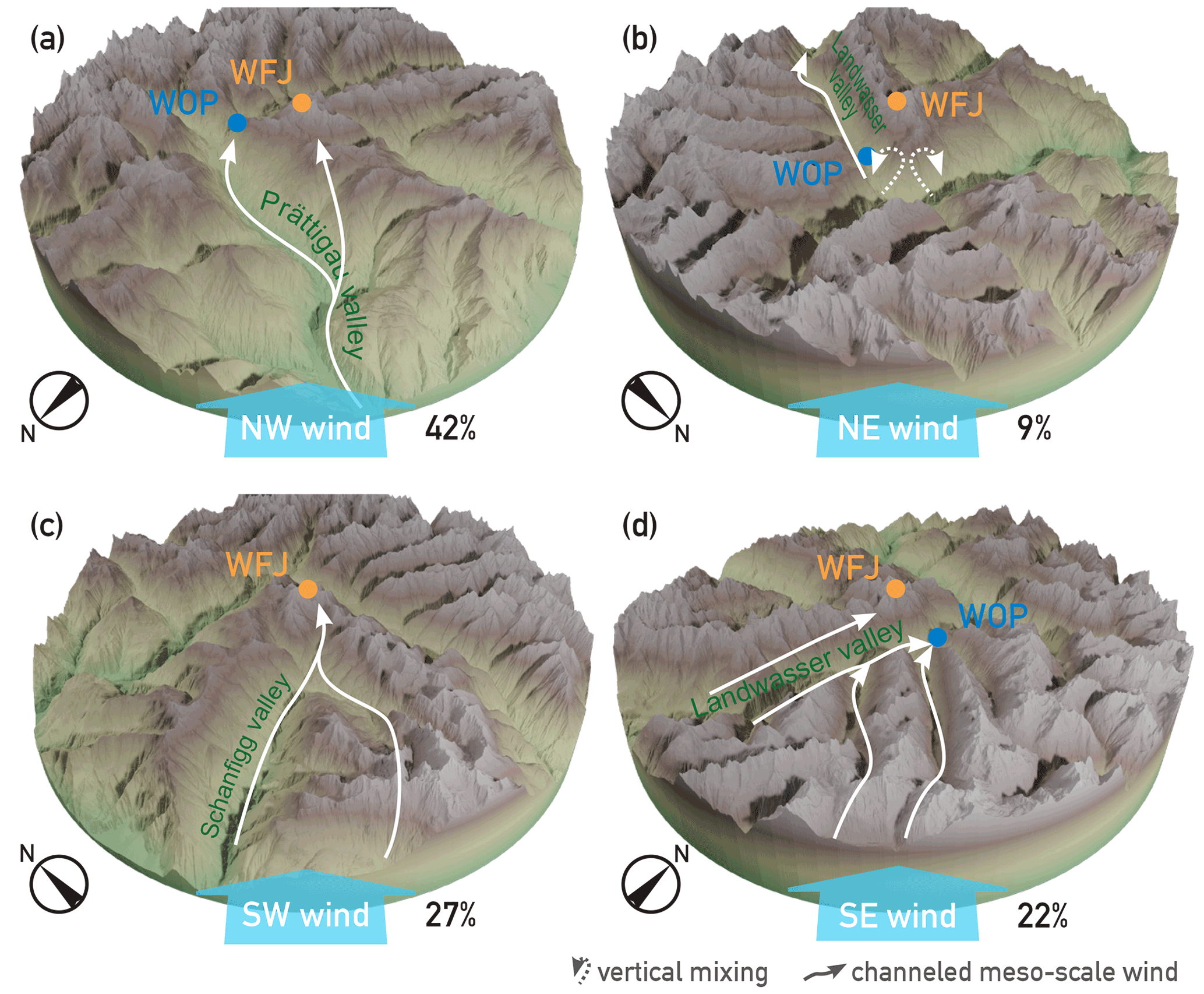
Figure 6Channeled winds in the valleys (solid white arrows) of the mesoscale winds (light blue arrows) for the topography around the two measurement sites (WFJ – orange dot; WOP – blue dot) within a radius of 20 km around WFJ for the four wind direction sectors (as defined in Fig. 1). The viewpoint in each panel is aligned with the mesoscale wind direction, is centered on WFJ (2693 ), and reaches down to an elevation of 500 The percentage of INP samples collected for each wind sector is indicated in the lower right of each subplot. In the NE wind case (b), the potential vertical mixing (i.e., rising of air masses originating from the valley and mixing with the air masses aloft) due to the conditional instability of the narrow cross-valley air masses is shown (dashed white arrows). The elevation data were obtained from the digital height model DHM2 from the Federal Office of Topography, swisstopo.
3.4 Assessing air mass transport using the Froude number
The regime for air mass transport towards and over a mountain barrier can be estimated by the Froude number Fr, as defined by the following ratio:
which is the synoptic wind speed U∞ to the barrier height h times the Brunt–Väisälä frequency N. For Fr≪1, the flow is blocked and transport over the barrier is hampered. If Fr>1, air masses are transported over the barrier. This means that, with increasing Fr, transport of air masses from upstream of the barrier to downstream is promoted. In Fig. 7, we present the WFJ INP concentration at −12 ∘C as a function of Fr for the four wind direction sectors. For the calculation of Fr, the wind speed measured at WFJ was used, which was found to be representative for the mesoscale flow. The difference in altitude of the subsequently described weather stations was used as the barrier height (h) per wind sector. The Brunt–Väisälä frequency was calculated using the meteorological data from WFJ and the respective upstream weather station in each sector (RAG for NW, ARO for SW, and DAV for SE and NE; see Fig. 1). For this approach, we made the assumption that using data from two weather stations located up to 30 km apart (distance WFJ–RAG) results in representative vertical gradients of pressure, relative humidity, and temperature. We could validate this assumption for the NW wind direction sector using meteorological data from the MeteoSchweiz weather station at Zurich airport (Kloten; 115 km NW of WFJ) as the lower reference point. The calculated Brunt–Väisälä frequencies using the data from WFJ–RAG and WFJ–Zurich airport resulted in similar values (a significant Pearson correlation coefficient of r=0.84), corroborating our understanding of air masses being pushed both from the Swiss plain over the Alps as a whole and locally from the Rhine valley to WFJ. It is clear that vertical transport will be suppressed in the presence of an inversion layer; however, as our measurements were performed during cloud events, we attribute the likelihood of such layers over the measurement period(s) as minor. For the cases of mesoscale NW and SW wind (Fig. 7a and c), we observed a significant moderate relation between INP concentration at −12 ∘C and Fr, which is in contrast to the NE and SE directions (Fig. 7b and d). This observation was indeed similar for INP concentrations at all temperatures between −8 and −16 ∘C (see Table A2). We attribute the positive relation between INP concentration and Fr to the NW and SW topography, such that the orographic lifting of air masses from the Rhine valley to WFJ occurs. Despite the absence of a significant or strong relation for the SE case, one observation can still be made. With increasing INP concentration at WFJ, the average INP ratio (average ratio between available INP concentrations between −10 and −14 ∘C at WFJ and WOP; see Eq. 5) increases. The increase in the average INP ratio indicates that, during mesoscale SE wind, air masses always reach WOP (i.e., INP ratio being independent of the Froude number but proportional to the INP concentration at WFJ) and, to a varying degree, WFJ (Fig. 7d). In the NW and SW cases, higher average INP ratios were also often found to coincide with a higher INP concentration at WFJ. Thus, on average, INP concentrations at WFJ were rarely higher than at WOP, and the increase in INP concentration at WFJ is larger than at WOP during air mass transport from NW and SW. This further supports the conclusion that the INP concentration at WFJ is more susceptible to aerosol perturbation. In the next section, we will discuss the mixing of air masses between WFJ and WOP for all wind direction sectors in more detail.
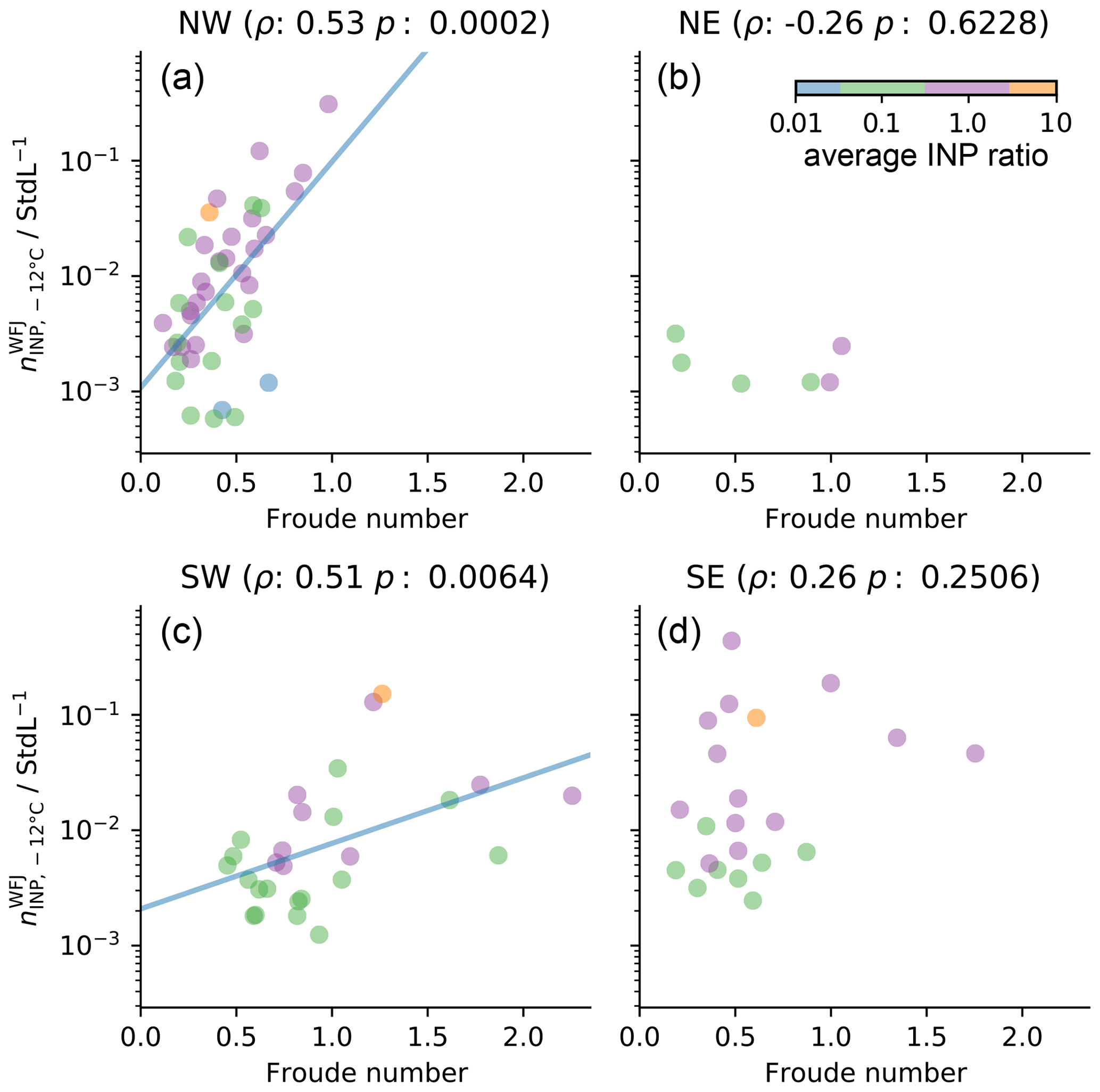
Figure 7INP concentration at −12 ∘C at WFJ () as a function of the Froude number (see Eq. 4) for the four mesoscale wind direction sectors (as indicated in Fig. 1). For each subplot, the Spearman's rank coefficient (ρ) and the corresponding two-sided p value (p) are shown at the top. The colors of the dots indicate the average INP ratio between WFJ and WOP (to assess the similarity of the INP concentration of both sites), as defined in Eq. (5). Lines are exponential fits in the case of 0.5.
3.5 Vertical mixing of air masses
To assess the vertical stability and mixing of the lower troposphere in the absence of clouds, the gradient of the potential temperature θ is typically utilized. It accounts for decreasing atmospheric pressure with increasing altitude, resulting in decreasing air density. Air masses are stably layered if θ increases with altitude (see, e.g., Stull, 1988). In the opposite case of unstable layering, air masses with higher θ rise until the negative θ gradient diminishes. Our measurements specifically targeted cloud events. Thus, to assess vertical stability, we utilized the equivalent potential temperature θe, which, in addition to pressure, also considers the latent heat that was released during condensation (Stull, 1988). To relate the INP concentrations measured at WFJ to WOP, we calculate a ratio between two samples collected synchronously at both sites. The ratio in INP concentration rINP,T at a given temperature T might not be available at all temperatures for a pair of samples (one from WOP and one from WFJ), as the overlap of available INP concentration varies between the samples. For example, if WOP experienced very ice-active air masses but not WFJ, then the INP concentrations at WOP could only be available down to −11 ∘C, whereas at WFJ INP concentrations could not be available above −10 ∘C. Thus, rINP,T would only be available at −10 and −11 ∘C. In other cases, rINP,T could only be available at −14 ∘C. Thus, to generally assess the similarity of the observed INP concentration, we take the mean of all available rINP,T between −10 and −14 ∘C, which is the temperature range in which INP concentrations at WOP and WFJ overlapped most (see Fig. 3). The average INP ratio was calculated as follows:
with ℳ being the set of all temperatures between −10 and −14 ∘C at which an INP concentration and was detectable at WFJ and WOP, respectively. In Fig. 8, we present the average INP ratio between WFJ and WOP per wind direction sector (see Fig. 1) as a function of the θe gradient with height. An upstream weather station in each wind direction sector was used to calculate θe at the valley floor (SRS for NW, ARO for SW, and DAV for SE and NE; see Fig. 1). The θe gradient was calculated by dividing the difference in θe between WFJ and the respective upstream weather station by the height difference of both stations.

Figure 8Average INP ratio (; as defined in Eq. 5) between synchronous INP samples taken at WFJ and WOP as a function of altitudinal θe gradient for each wind direction sector. The dashed (horizontal) line indicates an average INP ratio of 1. The dotted (vertical) line indicates θe gradient of 0, representing a neutrally layered lower atmosphere. For each sector, the Spearman's rank coefficient (ρ) and the corresponding two-sided p value (p) are shown at the top. The marker shape indicates the sampling time (morning, afternoon, and night; according to the time periods defined in Fig. 4). The color of the markers indicates the INP concentration at −12 ∘C measured at WFJ. Blue solid lines are exponential fits in case 0.5.
In the previous section, we presented evidence for the advective transport of INP-rich aerosol from a lower elevation to WFJ and WOP during a period with mesoscale westerly wind. For mesoscale NW wind, we observed a significant moderate correlation between the average INP ratio and the θe gradient (Fig. 8a), i.e., more similar INP concentrations coinciding with higher vertical stability. This finding renders the local mixing of air masses (e.g., by convection) unlikely but confirms the advection of the same air mass to the two sites as the underlying transport mechanism. Despite the similar topography, we did not observe this trend to the same extent for mesoscale SW wind (Fig. 8c). We attribute this to the fact that, for this wind direction, WOP is situated leeward of the mountain ridge around WFJ, and thus, the same air mass was not necessarily sampled at both sites. In the case of mesoscale NE wind, we observed increasingly coupled air masses between WFJ and WOP, with a decreasing θe gradient. This indicates that, for the NE topography, air masses from the valley can reach WFJ when the lower air masses are conditional unstably layered (see Fig. 6b). Strong convection as a transport mechanism seems unlikely in the wintertime Alps due to the extensive snow cover. However, a faster heating of the valley air masses was observed (possibly due to a lower surface albedo by vegetation such as conifers) for the days being analyzed that could lead to slight local instability. In the case of SE wind (Fig. 8d), no relation between the two variables was found, such that no specific transport mechanism could be identified. The SE topography illustrates that an assessment of the changes in INP concentration based on meteorological parameters requires a rather simple topography such as, e.g., a ramp-like structure in the NW case.
Previously, we presented the diurnal cycle of median INP concentrations at WFJ (see Fig. 5). In Fig. 8, it can be observed that high average INP ratios were not exclusively observed during the night. Advection, which is most likely the underlying transport mechanism of INPs in the NW and SW cases, is not necessarily strongest towards the end of the day but would vary depending on the mesoscale flow. However, the distribution of the average INP ratios per period for the NW and SW cases exhibits the trend of progressively more similar INP concentrations at both sites over the course of the day, which is resembled in the diurnal cycle at WFJ (Fig. 5). Apart from a strong enough advection itself, the INP concentrations at WFJ likely depend on the air mass history and their potential INP uptake upstream of the site. In the next section, we will examine the locations of potential INP uptake by the air masses arriving at WFJ.
3.6 Connecting transport mechanisms to observed diurnal cycle
For all samples considered in this study, the majority (69 %) were collected during synoptic westerly wind situations (NW and SW cases combined; see Fig. 7a and c) during which orographic lifting is the dominant transport mechanism of INPs towards WFJ. Thus, the diurnal cycle observed at WFJ (Fig. 4) is likely a result of three phenomena that are superimposed to varying degrees over the course of a day. These are (i) the strength of advection of an air mass towards WFJ, (ii) the residual time of an air mass close to INP sources, and (iii) the strength of INP sources at the time the air mass passed. In the previous sections, we presented that, in situations of westerly wind, higher INP concentrations at WFJ coincided with signs of stronger advection. To assess the locations of potential sources and, thus, the potential uptake of INPs by air masses measured at WFJ, we present INP footprint maps on a regional scale in Fig. 9 and on a global scale in Fig. A3. Locations of potential INP sources are indicated with a circle, where the 10 min time steps of a back-trajectory was less than 500 m above ground, and only for altitudes less than 2500 , which we assume to be relevant for INP uptake. On a global scale, we could not identify preferred INP source locations of air masses for the three time periods (Fig. A3). Note that INP contributions from long-range transport, such as Saharan dust, are unlikely due to the selection of the analyzed samples (see Sect. 2.1.1). Thus, we constrain our further analysis to potential source locations on the regional scale. Back-trajectories related to INP measurements in the morning (Fig. 9a) frequently passed over the Swiss plateau and, generally, low INP concentrations were measured at WFJ. For INP measurements in the afternoon (Fig. 9b), low trajectory heights above ground were found in rather close proximity to WFJ. Thus, the increasing INP concentrations during this time could be attributed to local sources from the surrounding valleys. Following Huang et al. (2021) and Kanji et al. (2017), potential sources of INP active above −20 ∘C are bioaerosols (bacteria, fungi, and leaf litter), lofted soil dust, and pollen emissions of the lower-lying land which was not fully snow covered at the time of measurement. From February onward, hazel and alder are common in the Davos region (MeteoSchweiz, 2021a) and even more so in the Rhine valley (MeteoSchweiz, 2021b). Starting in March, poplar, ash, and birch also contribute to the pollen population. Anthropogenic activities such as biomass burning, industrial processes and transportation also contributed to the aerosol population but are not thought to contribute to the increased INP concentration and activated fraction, as discussed in Sect. 3.2. In addition, the local boundary layer height could have already increased by noon, such that aerosol could be brought to higher altitudes over the Rhine valley, potentially increasing the minimal height for aerosol uptake by a passing air mass. For INP measurements during the night (Fig. 9c), trajectories originated again over the Swiss plateau, and high INP concentrations were observed. In contrast to the morning, air masses moved slower (smaller distances between individual circles in Fig. 9c) and, thus, spent more time at low heights over the Swiss plateau. Consequently, more aerosol from the PBL over the Swiss plateau could be taken up by the air masses, given the longer residence time at lower altitude. Due to the lower altitude and larger agricultural areas, the contributions of bioaerosol and soil dust, respectively, can be assumed to be stronger. In addition, the pollen season had already begun (MeteoSchweiz, 2021c) in January. From this, we conclude that, during the synoptic west wind, an increasing concentration of INPs was potentially transported by advection towards WFJ over the course of a day. While their origin at the beginning of the day was more likely to be within the closer proximity upstream of WFJ, aerosol sourced in the Swiss plateau could also have contributed to the observed INP concentrations in the evening and at night.
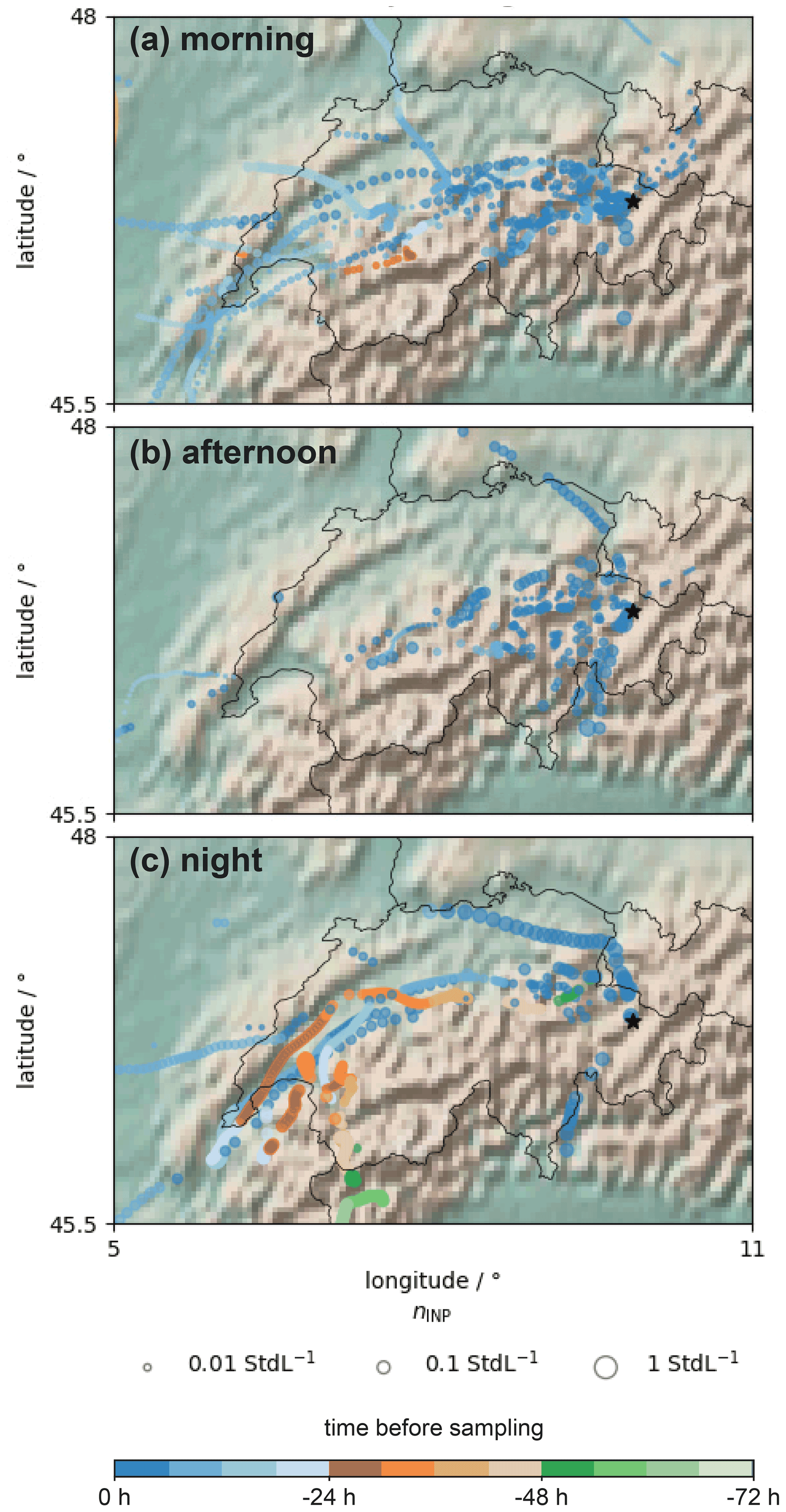
Figure 9Footprint maps of potential INP uptake locations derived from back-trajectories associated with INP samples (one trajectory per sample) taken at WFJ for the periods in the morning (a), afternoon (b), and at night (c). The circles indicate locations where a trajectory's 10 min time step was lower than 500 m above ground (and the surface height less than 2500 ). The color of a circle indicates the time before the corresponding air mass was sampled at WFJ. The size of a circle is proportional to the INP concentration at −12 ∘C measured at WFJ. The black star indicates the location of WFJ. The shaded relief was plotted with the Python basemap library.
In this study, we investigated the spatiotemporal distribution of INPs over the Swiss Alps near Davos in February and March 2019. Our analysis was based on simultaneous in situ INP measurements between 0 to −20 ∘C using offline drop-freezing techniques on site and aerosol size distribution measurements in a high valley and on a nearby mountaintop. We used the vertical gradient in equivalent potential temperature and the Froude number around the measurement sites to identify atmospheric mixing and transport process regimes, respectively. Source regions of advective transport were suggested based on back-trajectory footprint maps. After studying the diurnal variations in INP concentration at both sites during cloud events, we conclude the following:
-
The median INP concentrations measured throughout the field campaign in February and March 2019 on Weissfluhjoch (WFJ) were lower than in the high valley at Wolfgangpass (WOP) by a factor of approximately 3 across the temperature spectrum. The distributions of INP concentrations measured at WFJ show a larger variability which, together with the lower median INP concentrations, makes WFJ more susceptible to perturbations of INP (local sources or transported long-range).
-
The median INP concentrations at WFJ increased by nearly 1 order of magnitude over the course of a day, equilibrating to the concentrations measured at WOP, where median INP concentrations did not substantially change over the course of a day.
-
We found significant correlations between the Froude number and the INP concentrations for periods with mesoscale wind directions from NW and SW, which indicates a transport of low-level valley air masses to the mountain top site by forced orographic lifting. This finding could be generally true for a topography if the mesoscale wind direction aligns to the valley axis.
-
We deduced that, in the situation of a mesoscale wind perpendicular to a mountain valley, INP concentration on the mountaintop downstream can increase if the valley air masses are (conditional) unstable. The extent of this mechanism could not be shown with full significance, due to a low number of available samples with these conditions.
-
The dominant transport mechanism across all observations was advection, followed by orographic lifting. The resulting response in INP concentration observed on the mountaintop depends on (i) the strength of advection of air masses and (ii) the upstream residual time of the air masses close within the PBL at low altitude. We conclude that INP-rich air masses are being pushed from the upstream valley and plains to the mountain ridge over the course of a day (Fig. 6). Whereas the advected INPs originate from the surrounding valleys during the day, they source from the Swiss plateau towards the night.
Additionally, we note the variability in the observed activated fraction, i.e., the absence of a relation between INP concentration and the aerosol (number) concentration (see Appendix A3). It implies that predicting continental INP concentrations at warmer temperatures ( ∘C; observed temperature range in this study), based on aerosol number concentration alone, can be uncertain and that dynamics play the dominant role, especially over orographic terrain. Our study suggests that, over orographic terrain and during strong mesoscale winds over the Alps, mountaintop INP concentrations adjust to the INP concentrations of the valleys upstream over the course of a day. Thus, scaling existing INP parameterizations by an advective transport variable, such as the Froude number used in this study, could lead to a more accurate representation of INP in model applications. To study INP transport mechanisms, gathering high-resolution datasets of INP concentrations is of crucial importance. Despite the labor-intensive work associated with using offline methods, this could be done at two nearby sites in this study. Recent developments gave rise to different autonomous online INP counters (Bi et al., 2019; Brunner and Kanji, 2021; Möhler et al., 2021). Installing several units of these instruments in regions of interest can be used to improve the understanding of INP transport mechanisms in future studies. At the moment, the minimal detectable concentrations and maximal operation temperatures are not suitable for studying INPs at warm temperatures ( ∘C, Brunner and Kanji, 2021), but a next generation of online counters may overcome these limitations.
A1 INP concentrations at WFJ per wind direction
To assess the potential influence of the restaurant west of the sampling site of WFJ, we show INP concentrations at different temperatures as a function of wind direction in Fig. A1. An influence from the cooking for lunch would be expected from the west and between 10:00 and 13:00 LT. No significant increase in INP concentration matching the two criteria was observed, rendering a contribution from cooking emissions minuscule.
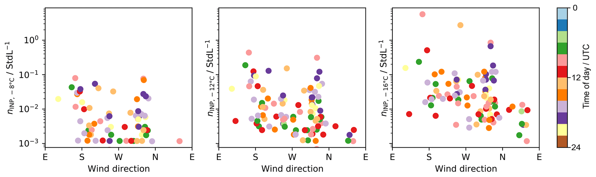
Figure A1INP concentrations at −8, −12, and −16 ∘C measured at WFJ as a function of wind direction. The color indicates the time of sampling.
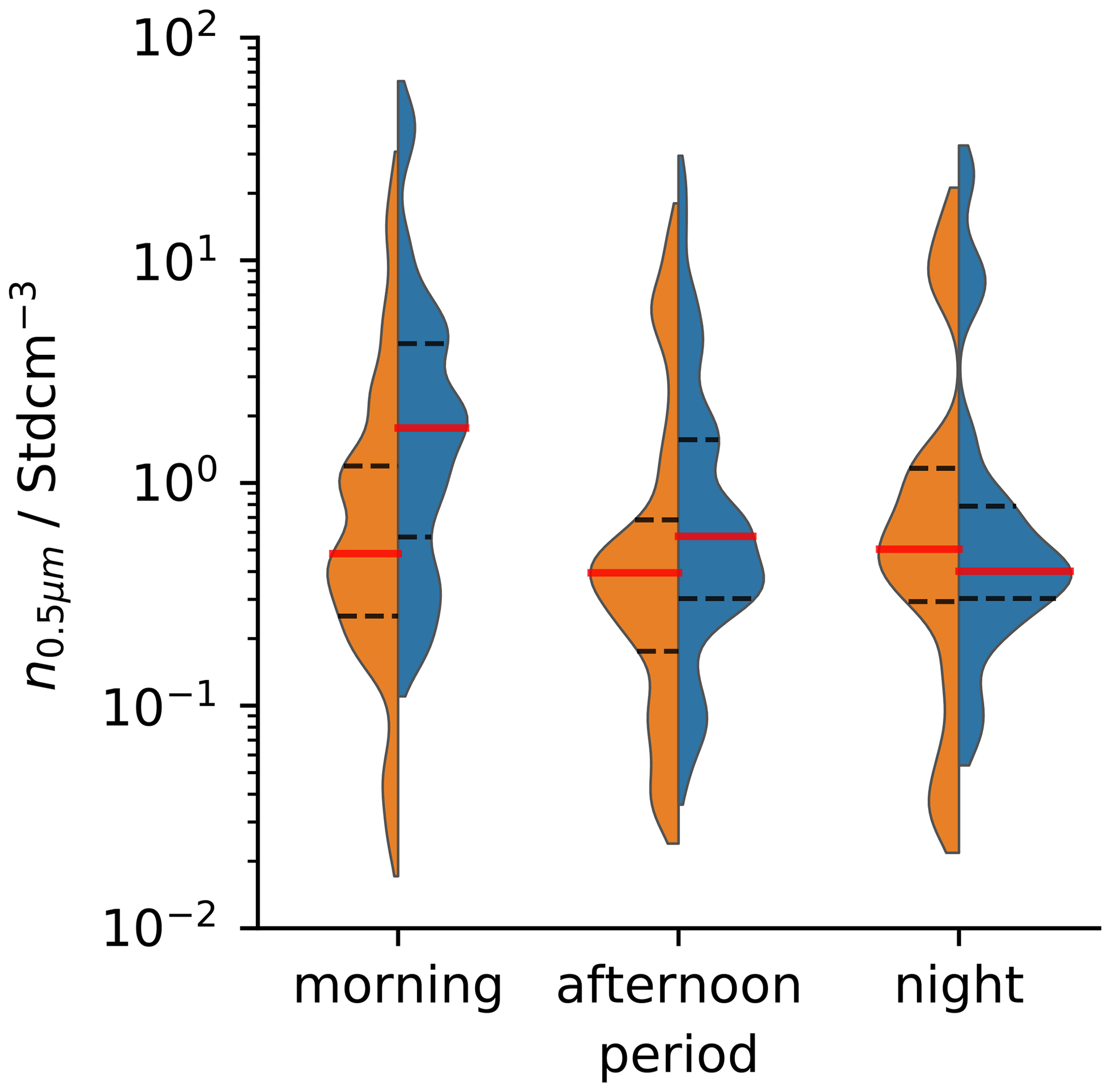
Figure A2Violin plots of aerosol number concentrations for particles with a physical diameter larger than 0.5 µm (n0.5 µm) at WFJ (orange) and WOP (blue) in the morning (03:00–11:59 UTC), the afternoon (12:00–17:59 UTC), and at night (18:00–02:59 UTC). Only measurements that coincide with INP samples at each side have been included.
A2 Aerosol concentrations during investigated periods
Violin plots of the aerosol number concentrations with physical diameters larger than 0.5 µm during sampling for INP analysis at both sites for the morning, afternoon and night period (see Sect. 2.1.1) are shown in Fig. A2. While the median concentration at WFJ is relatively stable, it decreases at WOP by roughly a factor of 5 from the morning to the night. In addition, the shape of the distributions at WFJ and WOP also becomes similar at night, indicating a better mixing of the atmosphere between the high valley and the mountaintop. We validated that the difference in aerosol number concentration between individual samples measured in parallel at WFJ and WOP does indeed become the smallest during the night.
A3 Correlation coefficients of INP concentration at different temperature versus aerosol number concentration
Figure 5 suggests the absence of a relation between the INP concentration and aerosol number concentration. Table A1 summarizes the correlation coefficients between the INP concentration across the observed temperature range and aerosol number concentration. In some cases (e.g., at WFJ at night for temperatures from −14 to −16 ∘C), a stronger and more significant relation was found. However, based on the entire dataset, the aerosol number concentration does not seem to be a good predictor for the INP concentration as a stable relation was not found. In turn, a stable and significant relation for INP concentration observed at WFJ was found with the Froude number for certain wind directions (see Sect. A4).
Table A1Spearman's rank coefficients (ρ) between aerosol number concentration for particles with physical diameter larger than 0.5 µm (n0.5 µm) and INP concentration at different temperatures (−7 to −18 ∘C) at WOP and WFJ for the three periods in the morning (03:00–11:59 UTC), afternoon (12:00–17:59 UTC), and at night (18:00–02:59 UTC). Numbers in bold represent a significant result (two-sided p<0.05).
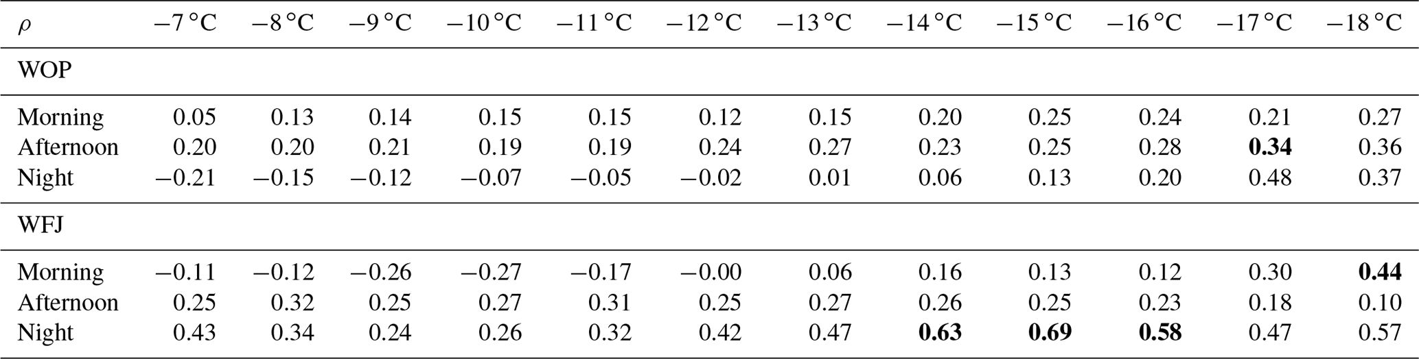
Table A2Spearman's rank coefficients (ρ) between the Froude number and INP concentrations at different temperatures (−7 to −18 ∘C) per wind sector (see Fig. 1). Numbers in bold represent a significant result (two-sided p<0.05). At −7 ∘C, only two INP concentrations were available at NE, such that no Spearman's rank coefficient could be calculated.

A4 Correlation coefficients of WFJ INP concentration at different temperature versus Froude number
The transport of INP towards WFJ was assessed using the Froude number. Table A2 summarizes Spearman's rank coefficients (ρ) between the Froude number and WFJ INP concentrations at temperatures between −7 and −18 ∘C (in the main text, only the results for INP concentrations at −12 ∘C were shown). A continuous range of significant relations was found for synoptic NW and SW wind (see Fig. 1) between −8 and −16 ∘C.
A5 Diurnal global back-trajectory maps
Figure A3 shows the back-trajectories associated with all samples at WFJ for the morning, afternoon, and night periods (see Sect. 2.1.1). No preferential source region could be identified on a global scale.

Figure A3Footprint map calculated from back trajectories of each sample taken at WFJ for the periods in the morning (a), afternoon (b), and at night (c), as defined in Sect. 2.1.1. The dots indicate places where the trajectories were lower than 500 m above ground. The number of trajectories per plot (N) is listed in the upper right corner of each plot. The black star indicates the location of WFJ.
The code is available on request to the authors. The data obtained within RACLETS used in this study are published on the campaign's website (https://www.envidat.ch/raclets-field-campaign, last access: 6 March 2022) and can be accessed via https://www.envidat.ch/dataset/aerosol-data-davos-wolfgang (last access: 6 March 2022, https://doi.org/10.16904/envidat.157, Wieder and Rösch, 2020), https://www.envidat.ch/dataset/aerosol-data-weissfluhjoch (last access: 6 March 2022, https://doi.org/10.16904/envidat.156, Wieder et al., 2020), and https://www.envidat.ch/dataset/raclets-backward-trajectories (last access: 6 March 2022, https://doi.org/10.16904/envidat.120, Sprenger, 2019). The meteorological data at Wolfgangpass are accessible via https://www.envidat.ch/dataset/weather-station-wolfgangpass (last access: 6 March 2022, https://doi.org/10.16904/envidat.137, Wieder, 2020). The meteorological data at Arosa, Bad Ragaz, Davos Dorf, Schiers, and Weissfluhjoch, can be requested using the IDAWEB application of MeteoSchweiz (https://www.gate.meteoswiss.ch/idaweb/, last access: 6 March 2022).
JW performed the analysis and prepared the figures for the paper. JW and CM installed and maintained the aerosol instruments in Davos. JW, CM, MaS, and LR performed the aerosol measurements during the campaign. MiS provided the back-trajectory data and helped with their analysis. CB processed the topographic data from the DHM2 model. JW, CM, JH, UL, CB, and ZAK interpreted the data. JW wrote the paper, with contributions from all co-authors. All authors reviewed the paper. ZAK supervised the project.
The contact author has declared that neither they nor their co-authors have any competing interests.
Publisher's note: Copernicus Publications remains neutral with regard to jurisdictional claims in published maps and institutional affiliations.
The authors express their gratitude to the RACLETS campaign team, for their technical support and many fruitful discussions. In particular, we thank Michael Lehning (WSL/SLF; EPFL) and his team, for their support in realizing the RACLETS campaign. We thank Paul Fopp, for providing his land at Wolfgangpass, and Martin Genter, for the logistical support at Weissfluhjoch. Our deepest appreciation to Michael Rösch and Marco Vecellio, for the technical support. We express our deepest gratitude to Nora Els (University of Innsbruck), for providing us with a second impinger. We thank MeteoSchweiz, for the meteorological observations. The authors thank Franz Conen, Robert O. David, Alexandra Moniz, Fabiola Ramelli, Carolin Rösch, Maxim Samarin, and Colin Tully, for the discussions and suggestions that improved the paper. Furthermore, the authors want to thank the two anonymous reviewers, for their comments and suggestions, which improved the paper.
This research has been supported by the Schweizerischer Nationalfonds zur Förderung der Wissenschaftlichen Forschung (grant nos. 200021_169620 and 200021_175824).
This paper was edited by Corinna Hoose and reviewed by two anonymous referees.
Baldauf, M., Seifert, A., Förstner, J., Majewski, D., Raschendorfer, M., and Reinhardt, T.: Operational convective-scale numerical weather prediction with the COSMO model: Description and sensitivities, Mon. Weather Rev., 139, 3887–3905, https://doi.org/10.1175/MWR-D-10-05013.1, 2011. a
Barry, R. G. and Chorley, R. J.: Atmosphere, Weather and Climate, 8th Edn., ISBN 9780203428238, 2003. a
Baumann, K., Maurer, H., Rau, G., Piringer, M., Pechinger, U., Prévôt, A., Furger, M., Furger, M., Neininger, B., and Pellegrini, U.: The influence of south Foehn on the ozone distribution in the Alpine Rhine valley – results from the MAP field phase, Atmos. Environ., 35, 6379–6390, 2001. a
Beck, A., Henneberger, J., Schöpfer, S., Fugal, J., and Lohmann, U.: HoloGondel: in situ cloud observations on a cable car in the Swiss Alps using a holographic imager, Atmos. Meas. Tech., 10, 459–476, https://doi.org/10.5194/amt-10-459-2017, 2017. a
Bi, K., McMeeking, G. R., Ding, D. P., Levin, E. J., DeMott, P. J., Zhao, D. L., Wang, F., Liu, Q., Tian, P., Ma, X. C., Chen, Y. B., Huang, M. Y., Zhang, H. L., Gordon, T. D., and Chen, P.: Measurements of Ice Nucleating Particles in Beijing, China, J. Geophys. Res.-Atmos., 124, 8065–8075, https://doi.org/10.1029/2019JD030609, 2019. a
Boose, Y., Kanji, Z. A., Kohn, M., Sierau, B., Zipori, A., Crawford, I., Lloyd, G., Bukowiecki, N., Herrmann, E., Kupiszewski, P., Steinbacher, M., and Lohmann, U.: Ice nucleating particle measurements at 241 K during winter months at 3580 m MSL in the swiss alps, J. Atmos. Sci., 73, 2203–2228, https://doi.org/10.1175/JAS-D-15-0236.1, 2016a. a
Boose, Y., Welti, A., Atkinson, J., Ramelli, F., Danielczok, A., Bingemer, H. G., Plötze, M., Sierau, B., Kanji, Z. A., and Lohmann, U.: Heterogeneous ice nucleation on dust particles sourced from nine deserts worldwide – Part 1: Immersion freezing, Atmos. Chem. Phys., 16, 15075–15095, https://doi.org/10.5194/acp-16-15075-2016, 2016b. a
Borys, R. D., Lowenthal, D. H., Cohn, S. A., and Brown, W. O.: Mountaintop and radar measurements of anthropogenic aerosol effects on snow growth and snowfall rate, Geophys. Res. Lett., 30, 1538, https://doi.org/10.1029/2002gl016855, 2003. a
Brunner, C. and Kanji, Z. A.: Continuous online monitoring of ice-nucleating particles: development of the automated Horizontal Ice Nucleation Chamber (HINC-Auto), Atmospheric Measurement Techniques, 14, 269–293, https://doi.org/10.5194/amt-14-269-2021, 2021. a, b, c
Chen, J., Wu, Z., Augustin-Bauditz, S., Grawe, S., Hartmann, M., Pei, X., Liu, Z., Ji, D., and Wex, H.: Ice-nucleating particle concentrations unaffected by urban air pollution in Beijing, China, Atmos. Chem. Phys., 18, 3523–3539, https://doi.org/10.5194/acp-18-3523-2018, 2018. a
Chou, C., Kanji, Z. A., Stetzer, O., Tritscher, T., Chirico, R., Heringa, M. F., Weingartner, E., Prévôt, A. S. H., Baltensperger, U., and Lohmann, U.: Effect of photochemical ageing on the ice nucleation properties of diesel and wood burning particles, Atmos. Chem. Phys., 13, 761–772, https://doi.org/10.5194/acp-13-761-2013, 2013. a
Chow, F. K., Wekker, S. F. D., and Snyder, B. J.: Mountain Weather Research and Mountain Weather Research and Forecasting: Recent Progress and Current Challenges, Springer Atmospheric Sciences, https://link.springer.com/book/10.1007/978-94-007-4098-3 (last access: 21 February 2022), 2013. a, b, c, d, e, f, g
Conen, F., Rodríguez, S., Hüglin, C., Henne, S., Herrmann, E., Bukowiecki, N., and Alewell, C.: Atmospheric ice nuclei at the high-altitude observatory Jungfraujoch, Switzerland, Tellus Ser. B, 67, 25014, https://doi.org/10.3402/tellusb.v67.25014, 2015. a
Conen, F., Yakutin, M. V., Yttri, K. E., and Hüglin, C.: Ice nucleating particle concentrations increase when leaves fall in autumn, Atmosphere, 8, 202, https://doi.org/10.3390/atmos8100202, 2017. a, b
Creamean, J. M., Mignani, C., Bukowiecki, N., and Conen, F.: Using freezing spectra characteristics to identify ice-nucleating particle populations during the winter in the Alps, Atmos. Chem. Phys., 19, 8123–8140, https://doi.org/10.5194/acp-19-8123-2019, 2019. a
David, R. O., Cascajo-Castresana, M., Brennan, K. P., Rösch, M., Els, N., Werz, J., Weichlinger, V., Boynton, L. S., Bogler, S., Borduas-Dedekind, N., Marcolli, C., and Kanji, Z. A.: Development of the DRoplet Ice Nuclei Counter Zurich (DRINCZ): validation and application to field-collected snow samples, Atmos. Meas. Tech., 12, 6865–6888, https://doi.org/10.5194/amt-12-6865-2019, 2019. a, b, c
DeMott, P. J., Cziczo, D. J., Prenni, A. J., Murphy, D. M., Kreidenweis, S. M., Thomson, D. S., Borys, R., and Rogers, D. C.: Measurements of the concentration and composition of nuclei for cirrus formation, P. Natl. Acad. Sci. USA, 100, 14655–14660, https://doi.org/10.1073/pnas.2532677100, 2003. a
Demott, P. J., Prenni, A. J., Liu, X., Kreidenweis, S. M., Petters, M. D., Twohy, C. H., Richardson, M. S., Eidhammer, T., and Rogers, D. C.: Predicting global atmospheric ice nuclei distributions and their impacts on climate, P. Natl. Acad. Sci. USA, 107, 11217–11222, https://doi.org/10.1073/pnas.0910818107, 2010. a
DeMott, P. J., Prenni, A. J., McMeeking, G. R., Sullivan, R. C., Petters, M. D., Tobo, Y., Niemand, M., Möhler, O., Snider, J. R., Wang, Z., and Kreidenweis, S. M.: Integrating laboratory and field data to quantify the immersion freezing ice nucleation activity of mineral dust particles, Atmos. Chem. Phys., 15, 393–409, https://doi.org/10.5194/acp-15-393-2015, 2015. a
Envidat: RACLETS field campaign, https://www.envidat.ch/group/about/raclets-field-campaign, 2019. a
Field, P. R. and Heymsfield, A. J.: Importance of snow to global precipitation, Geophys. Res. Lett., 42, 9512–9520, https://doi.org/10.1002/2015GL065497, 2015. a
Georgakaki, P., Bougiatioti, A., Wieder, J., Mignani, C., Ramelli, F., Kanji, Z. A., Henneberger, J., Hervo, M., Berne, A., Lohmann, U., and Nenes, A.: On the drivers of droplet variability in alpine mixed-phase clouds, Atmos. Chem. Phys., 21, 10993–11012, https://doi.org/10.5194/acp-21-10993-2021, 2021. a, b
Hegerl, G. C., Black, E., Allan, R. P., Ingram, W. J., Polson, D., Trenberth, K. E., Chadwick, R. S., Arkin, P. A., Sarojini, B. B., Becker, A., Dai, A., and Durack, P. J. A.: Challenges in Quantifying Changes in the Global Water Cycle, B. Am. Meteorol. Soc., 96, 1097–1116, 2015. a
Henneberger, J., Fugal, J. P., Stetzer, O., and Lohmann, U.: HOLIMO II: a digital holographic instrument for ground-based in situ observations of microphysical properties of mixed-phase clouds, Atmos. Meas. Tech., 6, 2975–2987, https://doi.org/10.5194/amt-6-2975-2013, 2013. a
Heymsfield, A. J., Schmitt, C., Chen, C.-C.-J., Bansemer, A., Gettelman, A., Field, P. R., and Liu, C.: Contributions of the Liquid and Ice Phases to Global Surface Precipitation: Observations and Global Climate Modeling, J. Atmos. Sci., 77, 2629–2648, https://doi.org/10.1175/JAS-D-19-0352.1, 2020. a
Huang, S., Hu, W., Chen, J., Wu, Z., Zhang, D., and Fu, P.: Overview of biological ice nucleating particles in the atmosphere, Environ. Int., 146, 106197, https://doi.org/10.1016/j.envint.2020.106197, 2021. a, b, c, d
Huffman, J. A., Prenni, A. J., DeMott, P. J., Pöhlker, C., Mason, R. H., Robinson, N. H., Fröhlich-Nowoisky, J., Tobo, Y., Després, V. R., Garcia, E., Gochis, D. J., Harris, E., Müller-Germann, I., Ruzene, C., Schmer, B., Sinha, B., Day, D. A., Andreae, M. O., Jimenez, J. L., Gallagher, M., Kreidenweis, S. M., Bertram, A. K., and Pöschl, U.: High concentrations of biological aerosol particles and ice nuclei during and after rain, Atmos. Chem. Phys., 13, 6151–6164, https://doi.org/10.5194/acp-13-6151-2013, 2013. a
Kanji, Z. A., Ladino, L. A., Wex, H., Boose, Y., Burkert-Kohn, M., Cziczo, D. J., and Krämer, M.: Overview of Ice Nucleating Particles, Meteorol. Monogr., 58, 1.1–1.33, https://doi.org/10.1175/AMSMONOGRAPHS-D-16-0006.1, 2017. a, b, c, d, e
Kanji, Z. A., Welti, A., Corbin, J. C., and Mensah, A. A.: Black Carbon Particles Do Not Matter for Immersion Mode Ice Nucleation, Geophys. Res. Lett., 47, e2019GL086764, https://doi.org/10.1029/2019GL086764, 2020. a
Klein, H., Nickovic, S., Haunold, W., Bundke, U., Nillius, B., Ebert, M., Weinbruch, S., Schuetz, L., Levin, Z., Barrie, L. A., and Bingemer, H.: Saharan dust and ice nuclei over Central Europe, Atmos. Chem. Phys., 10, 10211–10221, https://doi.org/10.5194/acp-10-10211-2010, 2010. a
Lacher, L., Lohmann, U., Boose, Y., Zipori, A., Herrmann, E., Bukowiecki, N., Steinbacher, M., and Kanji, Z. A.: The Horizontal Ice Nucleation Chamber (HINC): INP measurements at conditions relevant for mixed-phase clouds at the High Altitude Research Station Jungfraujoch, Atmos. Chem. Phys., 17, 15199–15224, https://doi.org/10.5194/acp-17-15199-2017, 2017. a
Lacher, L., DeMott, P. J., Levin, E. J., Suski, K. J., Boose, Y., Zipori, A., Herrmann, E., Bukowiecki, N., Steinbacher, M., Gute, E., Abbatt, J. P., Lohmann, U., and Kanji, Z. A.: Background Free-Tropospheric Ice Nucleating Particle Concentrations at Mixed-Phase Cloud Conditions, J. Geophys. Res.-Atmos., 123, 10506–10525, https://doi.org/10.1029/2018JD028338, 2018. a
Ladino, L. A., Raga, G. B., Alvarez-Ospina, H., Andino-Enríquez, M. A., Rosas, I., Martínez, L., Salinas, E., Miranda, J., Ramírez-Díaz, Z., Figueroa, B., Chou, C., Bertram, A. K., Quintana, E. T., Maldonado, L. A., García-Reynoso, A., Si, M., and Irish, V. E.: Ice-nucleating particles in a coastal tropical site, Atmos. Chem. Phys., 19, 6147–6165, https://doi.org/10.5194/acp-19-6147-2019, 2019. a
Lauber, A., Henneberger, J., Mignani, C., Ramelli, F., Pasquier, J. T., Wieder, J., Hervo, M., and Lohmann, U.: Continuous secondary-ice production initiated by updrafts through the melting layer in mountainous regions, Atmos. Chem. Phys., 21, 3855–3870, https://doi.org/10.5194/acp-21-3855-2021, 2021. a
Lee, D. S., Kingdon, R. D., Garland, J. A., and Jones, B. M. R.: Parametrisation of the orographic enhancement of precipitation and deposition in a long-term, long-range transport model, Ann. Geophys., 18, 1447–1466, https://doi.org/10.1007/s00585-000-1447-2, 2000. a
Lehner, M. and Rotach, M. W.: Current challenges in understanding and predicting transport and exchange in the atmosphere over mountainous terrain, Atmosphere, 9, 276, https://doi.org/10.3390/atmos9070276, 2018. a
Lohmann, U., Henneberger, J., Henneberg, O., Fugal, J. P., Bühl, J., and Kanji, Z. A.: Persistence of orographic mixed-phase clouds, Geophys. Res. Lett., 43, 10512–10519, https://doi.org/10.1002/2016GL071036, 2016a. a
Lohmann, U., Lüönd, F., and Mahrt, F.: An Introduction to Clouds: From the Microscale to Climate, 1 Edn., Cambridge University Press, Cambridge, UK, 2016 a, b
Mahrt, F., Marcolli, C., David, R. O., Grönquist, P., Barthazy Meier, E. J., Lohmann, U., and Kanji, Z. A.: Ice nucleation abilities of soot particles determined with the Horizontal Ice Nucleation Chamber, Atmos. Chem. Phys., 18, 13363–13392, https://doi.org/10.5194/acp-18-13363-2018, 2018. a
Mason, R. H., Si, M., Chou, C., Irish, V. E., Dickie, R., Elizondo, P., Wong, R., Brintnell, M., Elsasser, M., Lassar, W. M., Pierce, K. M., Leaitch, W. R., MacDonald, A. M., Platt, A., Toom-Sauntry, D., Sarda-Estève, R., Schiller, C. L., Suski, K. J., Hill, T. C. J., Abbatt, J. P. D., Huffman, J. A., DeMott, P. J., and Bertram, A. K.: Size-resolved measurements of ice-nucleating particles at six locations in North America and one in Europe, Atmos. Chem. Phys., 16, 1637–1651, https://doi.org/10.5194/acp-16-1637-2016, 2016. a
McCluskey, C. S., DeMott, P. J., Prenni, A. J., Levin, E. J., McMeeking, G. R., Sullivan, A. P., Hill, T. C., Nakao, S., Carrico, C. M., and Kreidenweis, S. M.: Characteristics of atmospheric ice nucleating particles associated with biomass burning in the US: Prescribed burns and wildfires, J. Geophys. Res., 119, 10458–10470, https://doi.org/10.1002/2014JD021980, 2014. a
MeteoSchweiz: Pollenkalender Davos−Wolfgang 2001–2020, https://www.meteoschweiz.admin.ch/product/output/climate-data/pollen-count-processing/PDS/pollencalendar_PDS_G.pdf (last access: 21 February 2022), 2021a. a
MeteoSchweiz: Pollenkalender Buchs 2001–2020, https://www.meteoschweiz.admin.ch/product/output/climate-data/pollen-count-processing/PBU/pollencalendar_PBU_G.pdf (last access: 21 February 2022), 2021b. a
MeteoSchweiz: Pollenkalender Bern 2001–2020, https://www.meteoschweiz.admin.ch/product/output/climate-data/pollen-count-processing/PBE/pollencalendar_PBE_G.pdf (last access: 21 February 2022), 2021c. a
Mignani, C., Wieder, J., Sprenger, M. A., Kanji, Z. A., Henneberger, J., Alewell, C., and Conen, F.: Towards parameterising atmospheric concentrations of ice-nucleating particles active at moderate supercooling, Atmos. Chem. Phys., 21, 657–664, https://doi.org/10.5194/acp-21-657-2021, 2021. a, b, c, d, e, f, g, h
Miller, A. J., Brennan, K. P., Mignani, C., Wieder, J., David, R. O., and Borduas-Dedekind, N.: Development of the drop Freezing Ice Nuclei Counter (FINC), intercomparison of droplet freezing techniques, and use of soluble lignin as an atmospheric ice nucleation standard, Atmos. Meas. Tech., 14, 3131–3151, https://doi.org/10.5194/amt-14-3131-2021, 2021. a
Möhler, O., Adams, M., Lacher, L., Vogel, F., Nadolny, J., Ullrich, R., Boffo, C., Pfeuffer, T., Hobl, A., Weiß, M., Vepuri, H. S. K., Hiranuma, N., and Murray, B. J.: The Portable Ice Nucleation Experiment (PINE): a new online instrument for laboratory studies and automated long-term field observations of ice-nucleating particles, Atmos. Meas. Tech., 14, 1143–1166, https://doi.org/10.5194/amt-14-1143-2021, 2021. a
Mott, R., Daniels, M., and Lehning, M.: Atmospheric flow development and associated changes in turbulent sensible heat flux over a patchy mountain snow cover, J. Hydrometeorol., 16, 1315–1340, https://doi.org/10.1175/JHM-D-14-0036.1, 2015. a
Muhlbauer, A. and Lohmann, U.: Sensitivity Studies of Aerosol–Cloud Interactions in Mixed-Phase Orographic Precipitation, J. Atmos. Sci., 66, 2517–2538, https://doi.org/10.1175/2009JAS3001.1, 2009. a
Mülmenstädt, J., Sourdeval, O., Delanoë, J., and Quaas, J.: Frequency of occurrence of rain from liquid-, mixed-, and ice-phase clouds derived from A-Train satellite retrievals, Geophys. Res. Lett., 42, 6502–6509, https://doi.org/10.1002/2015GL064604, 2015. a
Murray, B. J., O'Sullivan, D., Atkinson, J. D., and Webb, M. E.: Ice nucleation by particles immersed in supercooled cloud droplets, Chem. Soc. Rev., 41, 6519–6554, https://doi.org/10.1039/C2CS35200A, 2012. a
Murray, B. J., Carslaw, K. S., and Field, P. R.: Opinion: Cloud-phase climate feedback and the importance of ice-nucleating particles, Atmos. Chem. Phys., 21, 665–679, https://doi.org/10.5194/acp-21-665-2021, 2021. a
Niemand, M., Möhler, O., Vogel, B., Vogel, H., Hoose, C., Connolly, P., Klein, H., Bingemer, H., Demott, P., Skrotzki, J., and Leisner, T.: A particle-surface-area-based parameterization of immersion freezing on desert dust particles, J. Atmos. Sci., 69, 3077–3092, https://doi.org/10.1175/JAS-D-11-0249.1, 2012. a
Nyeki, S., Kalberer, M., Colbeck, I., Wekker, S. D., Furger, M., Gäggeler, H. W., Kossmann, M., Lugauer, M., Steyn, D., Weingartner, E., Wirth, M., and Baltensperger, U.: Convective boundary layer evolution to 4 km asl over High-alpine terrain: Airborne lidar observations in the Alps, Geophys. Res. Lett., 27, 689–692, https://doi.org/10.1029/1999gl010928, 2000. a
Paramonov, M., Drossaart van Dusseldorp, S., Gute, E., Abbatt, J. P. D., Heikkilä, P., Keskinen, J., Chen, X., Luoma, K., Heikkinen, L., Hao, L., Petäjä, T., and Kanji, Z. A.: Condensation/immersion mode ice-nucleating particles in a boreal environment, Atmos. Chem. Phys., 20, 6687–6706, https://doi.org/10.5194/acp-20-6687-2020, 2020. a
Poltera, Y., Martucci, G., Collaud Coen, M., Hervo, M., Emmenegger, L., Henne, S., Brunner, D., and Haefele, A.: PathfinderTURB: an automatic boundary layer algorithm. Development, validation and application to study the impact on in situ measurements at the Jungfraujoch, Atmos. Chem. Phys., 17, 10051–10070, https://doi.org/10.5194/acp-17-10051-2017, 2017. a, b
Pruppacher, H. R. and Klett, J. D.: Microphysics of Clouds and Precipitation, 2nd Edn., Springer, Dordrecht, 954, https://doi.org/10.1007/978-0-306-48100-0, 2010. a, b
Ramelli, F., Henneberger, J., David, R. O., Bühl, J., Radenz, M., Seifert, P., Wieder, J., Lauber, A., Pasquier, J. T., Engelmann, R., Mignani, C., Hervo, M., and Lohmann, U.: Microphysical investigation of the seeder and feeder region of an Alpine mixed-phase cloud, Atmos. Chem. Phys., 21, 6681–6706, https://doi.org/10.5194/acp-21-6681-2021, 2021a. a, b
Ramelli, F., Henneberger, J., David, R. O., Lauber, A., Pasquier, J. T., Wieder, J., Bühl, J., Seifert, P., Engelmann, R., Hervo, M., and Lohmann, U.: Influence of low-level blocking and turbulence on the microphysics of a mixed-phase cloud in an inner-Alpine valley, Atmos. Chem. Phys., 21, 5151–5172, https://doi.org/10.5194/acp-21-5151-2021, 2021b. a
Richardson, M. S., DeMott, P. J., Kreidenweis, S. M., Cziczo, D. J., Dunlea, E. J., Jimenez, J. L., Thomson, D. S., Ashbaugh, L. L., Borys, R. D., Westphal, D. L., Casuccio, G. S., and Lersch, T. L.: Measurements of heterogeneous ice nuclei in the western United States in springtime and their relation to aerosol characteristics, J. Geophys. Res.-Atmos., 112, D02209, https://doi.org/10.1029/2006JD007500, 2007. a
Rosenfeld, D., Lohmann, U., Raga, G. B., O'Dowd, C. D., Kulmala, M., Fuzzi, S., Reissell, A., and Andreae, M. O.: Flood or Drought: How Do Aerosols Affect Precipitation?, Science, 321, 1309–1313, https://doi.org/10.1126/science.1160606, 2008. a, b
Rotach, M. W. and Zardi, D.: On the boundary-layer structure over highly complex terrain: Key findings from MAP, Q. J. Roy. Meteorol. Soc., 133, 937–948, https://doi.org/10.1002/qj.71, 2007. a
Schättler, U., G, D., and Schraff, C.: A Description of the Non‐hydrostatic Regional COSMO Model. Part I: Dynamics and Numerics, http://www.cosmo-model.org (last access: 21 February 2022), 2015. a
Schmidli, J. and Rotunno, R.: Mechanisms of along-valley winds and heat exchange over mountainous terrain, J. Atmos. Sci., 67, 3033–3047, https://doi.org/10.1175/2010JAS3473.1, 2010. a
Seifried, T. M., Bieber, P., Kunert, A. T., Schmale, D. G., Whitmore, K., Fröhlich-Nowoisky, J., and Grothe, H.: Ice nucleation activity of alpine bioaerosol emitted in vicinity of a birch forest, Atmosphere, 12, 779, https://doi.org/10.3390/atmos12060779, 2021. a
Sprenger, M.: Backward Trajectories, EnviDat [data set], https://doi.org/10.16904/envidat.120, 2019. a
Sprenger, M. and Wernli, H.: The LAGRANTO Lagrangian analysis tool – version 2.0, Geosci. Model Dev., 8, 2569–2586, https://doi.org/10.5194/gmd-8-2569-2015, 2015. a
Stopelli, E., Conen, F., Zimmermann, L., Alewell, C., and Morris, C. E.: Freezing nucleation apparatus puts new slant on study of biological ice nucleators in precipitation, Atmos. Meas. Tech., 7, 129–134, https://doi.org/10.5194/amt-7-129-2014, 2014. a, b
Stull, R. B.: An introduction to boundary layer meteorology, Springer, https://doi.org/10.1007/978-94-009-3027-8, 1988. a, b, c, d
Thomas, D. and Charvet, A.: An Introduction to Aerosols, Aerosol Fi, Elsevier, https://doi.org/10.1016/B978-1-78548-215-1.50001-9, 2017. a
Tignino, M.: Water, international peace, and security, Int. Rev. Red Cross, 92, 647–674, https://doi.org/10.1017/S181638311000055X, 2010. a
Vali, G.: Quantitative Evaluation of Experimental Results an the Heterogeneous Freezing Nucleation of Supercooled Liquids, J. Atmos. Sci., 28, 402–409, https://doi.org/10.1175/1520-0469(1971)028<0402:QEOERA>2.0.CO;2, 1971. a, b
Vali, G.: Revisiting the differential freezing nucleus spectra derived from drop-freezing experiments: methods of calculation, applications, and confidence limits, Atmos. Meas. Tech., 12, 1219–1231, https://doi.org/10.5194/amt-12-1219-2019, 2019. a, b
Vali, G., DeMott, P. J., Möhler, O., and Whale, T. F.: Technical Note: A proposal for ice nucleation terminology, Atmos. Chem. Phys., 15, 10263–10270, https://doi.org/10.5194/acp-15-10263-2015, 2015. a
Vergara-Temprado, J., Holden, M. A., Orton, T. R., O'Sullivan, D., Umo, N. S., Browse, J., Reddington, C., Baeza-Romero, M. T., Jones, J. M., Lea-Langton, A., Williams, A., Carslaw, K. S., and Murray, B. J.: Is Black Carbon an Unimportant Ice-Nucleating Particle in Mixed-Phase Clouds?, J. Geophys. Res.-Atmos., 123, 4273–4283, https://doi.org/10.1002/2017JD027831, 2018. a
Walter, B., Huwald, H., Gehring, J., Bühler, Y., and Lehning, M.: Radar measurements of blowing snow off a mountain ridge, The Cryosphere, 14, 1779–1794, https://doi.org/10.5194/tc-14-1779-2020, 2020. a
Wegener, A.: Thermodynamik der Atmosphäre, J. A. Barth Verlag, Leipzig, Germany, 331 pp., 1911. a, b
Weingartner, E., Nyeki, S., and Baltensperger, U.: Seasonal and diurnal variation of aerosol size distributions (10 < D < 750 nm) at a high-alpine site (Jungfraujoch 3580 m asl), J. Geophys. Res.-Atmos., 104, 26809–26820, https://doi.org/10.1029/1999JD900170, 1999. a
Wekker, S. F. D. and Kossmann, M.: Convective boundary layer heights over mountainous terrain – A review of concepts, Front. Earth Sci., 3, 1–22, https://doi.org/10.3389/feart.2015.00077, 2015. a, b, c, d
Wernli, H. and Davies, H. C.: A lagrangian‐based analysis of extratropical cyclones. I: The method and some applications, Q. J. Roy. Meteor. Soc., 123, 467–489, 1997. a
Wieder, J.: Weather Station Davos Wolfgang, EnviDat [data set], https://doi.org/10.16904/envidat.137, 2020. a
Wieder, J. and Rösch, C.: Aerosol Data Davos Wolfgang, EnviDat [data set], https://doi.org/10.16904/envidat.157, 2020. a
Wieder, J., Mignani, C., and Rösch, C.: Aerosol Data Weissfluhjoch, EnviDat [data set], https://doi.org/10.16904/envidat.156, 2020. a