Factors affecting precipitation formation and precipitation susceptibility of marine stratocumulus with variable above- and below-cloud aerosol concentrations over the Southeast Atlantic

Aerosol–cloud–precipitation interactions (ACIs) provide the greatest source of uncertainties in predicting changes in Earth's energy budget due to poor representation of marine stratocumulus and the associated ACIs in climate models. Using in situ data from 329 cloud profiles across 24 research flights from the NASA ObseRvations of Aerosols above CLouds and their intEractionS (ORACLES) field campaign in September 2016, August 2017, and October 2018, it is shown that contact between above-cloud biomass burning aerosols and marine stratocumulus over the Southeast Atlantic Ocean was associated with precipitation suppression and a decrease in the precipitation susceptibility (S_o) to aerosols. The 173 “contact” profiles with aerosol concentration (N_a) greater than 500 cm⁻³ within 100 m above cloud tops had a 50 % lower precipitation rate (R_p) and a 20 % lower S_o, on average, compared to 156 “separated” profiles with N_a less than 500 cm⁻³ up to at least 100 m above cloud tops.

Contact and separated profiles had statistically significant differences in droplet concentration (N_c) and effective radius (R_e) (95 % confidence intervals from a two-sample t test are reported). Contact profiles had 84 to 90 cm⁻³ higher N_c and 1.4 to 1.6 µm lower R_e compared to separated profiles. In clean boundary layers (below-cloud N_a less than 350 cm⁻³), contact profiles had 25 to 31 cm⁻³ higher N_c and 0.2 to 0.5 µm lower R_e. In polluted boundary layers (below-cloud N_a exceeding 350 cm⁻³), contact profiles had 98 to 108 cm⁻³ higher N_c and 1.6 to 1.8 µm lower R_e. On the other hand, contact and separated profiles had statistically insignificant differences between the average liquid water path, cloud thickness, and meteorological parameters like surface temperature, lower tropospheric stability, and estimated inversion strength. These results suggest the changes in cloud microphysical properties were driven by ACIs rather than meteorological effects, and adjustments to existing relationships between R_p and N_c in model parameterizations should be considered to account for the role of ACIs.

1 Introduction

Clouds drive the global hydrological cycle with an annual average precipitation rate of 3 mm d⁻¹ over the oceans (Behrangi et al., 2014). Marine stratocumulus cloud (MSC) is the most common cloud type with an annual coverage of 22 % over the ocean surface (Eastman et al., 2011). These low-level, boundary layer clouds typically exist over subtropical oceans in regions with large-scale subsidence such as the Southeast Atlantic Ocean (Klein and Hartmann, 1993). MSCs have higher reflectivity (albedo) than the ocean surface, which results in a strong, negative shortwave cloud radiative forcing (CRF) with a weak and positive longwave CRF (Oreopoulos and Rossow, 2011).

Low-cloud cover in the subsidence regions is negatively correlated with sea surface temperature (SST) (Eastman et al., 2011; Wood and Hartmann, 2006). CRF is thus sensitive to changes in SST, but there is a large spread in model estimates of CRF sensitivity (Bony and Dufresne, 2005). This provides uncertainty in the model estimates of Earth's energy budget in future climate scenarios (Trenberth and Fasullo, 2009). Uncertainty in the parameterization of boundary layer aerosol, cloud, and precipitation processes contributes to model uncertainties (Ahlgrimm and Forbes, 2014; Stephens et al., 2010).

MSC CRF is regulated by cloud processes that depend on cloud microphysical properties, like droplet concentration (N_c), effective radius (R_e), and liquid water content (LWC), and macrophysical properties, like cloud thickness (H) and liquid water path (LWP). These cloud properties can depend on the concentration, composition, and size distributions of aerosols, which act as cloud condensation nuclei. Under conditions of constant LWC, increases in aerosol concentration (N_a) can increase N_c and decrease R_e, strengthening the shortwave CRF (Twomey, 1974, 1977). A decrease in droplet sizes in polluted clouds can inhibit droplet growth from collision–coalescence and suppress precipitation intensity, resulting in lower precipitation rate (R_p), higher LWP, and increased cloud lifetime (Albrecht, 1989). In combination, these aerosol–cloud–precipitation interactions (ACIs) and the resulting cloud adjustments lead to an effective radiative forcing, termed ERF_aci (Boucher et al., 2013).

Satellite retrievals of R_e and cloud optical thickness (τ) can be used to estimate N_c and LWP using the adiabatic assumption (Boers et al., 2006; Wood and Hartmann, 2006; Bennartz, 2007). LWC increases linearly with height in adiabatic clouds, and τ is parameterized as a function of N_c and LWP ($\mathit{\tau }\mathit{\alpha }{N}_{\mathrm{c}}^{\mathrm{1}/\mathrm{3}}$LWP${}^{\mathrm{5}/\mathrm{6}}$) (Brenguier et al., 2000). Since τ has greater sensitivity to LWP compared to N_c, assuming constant LWP under different aerosol conditions can lead to underestimation of the cloud albedo susceptibility to aerosol perturbations (Platnick and Twomey, 1994; McComiskey and Feingold, 2012).

LWP can have a positive or negative response to increasing N_c due to aerosols (Toll et al., 2019). The LWP response is regulated by environmental conditions (e.g., lower tropospheric stability (LTS), boundary layer depth (H_BL), and relative humidity), cloud particle sizes (e.g., represented by R_e), R_p, and by N_c and LWP themselves (Chen et al., 2014; Gryspeerdt et al., 2019; Toll et al., 2019; Possner et al., 2020). Accurate estimation of the LWP response to aerosol perturbations is important for regional and global estimates of ERF_aci (Douglas and L'Ecuyer, 2019, 2020).

Droplet evaporation associated with cloud-top entrainment and precipitation constitutes the two major sinks of LWC in MSC. Smaller droplets associated with higher N_c or N_a evaporate more readily, which leads to greater cloud-top evaporative cooling and a negative LWP response (Hill et al., 2008). The LWP response to the evaporation–entrainment feedback (Xue and Feingold, 2006; Small et al., 2009) also depends on above-cloud humidity (Ackerman et al., 2004). Precipitation susceptibility (S_o) to aerosol-induced changes in cloud properties is related to the change in R_p due to aerosol-induced changes in N_c and is a function of LWP or H (Feingold and Seibert, 2009).

The magnitude of S_o depends on precipitation formation processes like collision–coalescence which are parameterized in models using mass transfer rates, such as the autoconversion rate (S_AUTO) and the accretion rate (S_ACC) (Morrison and Gettelman, 2008; Geoffroy et al., 2010). Autoconversion describes the process of collisions between cloud droplets that coalesce to form drizzle drops which initiate precipitation. Accretion refers to collisions between cloud droplets and drizzle drops which lead to larger drizzle drops and greater precipitation intensity. The variability in S_o as a function of LWP or H depends on the cloud type and the ratio of S_ACC versus S_AUTO (Wood et al., 2009; Jiang et al., 2010; Sorooshian et al., 2010).

Recent field campaigns focused on studying ACIs over the Southeast Atlantic Ocean because unique meteorological conditions are present in the region (Zuidema et al., 2016; Redemann et al., 2021). Biomass burning aerosols from southern Africa are lofted into the free troposphere (Gui et al., 2021) and transported over the Southeast Atlantic by mid-tropospheric winds where the aerosols overlay an extensive MSC deck that exists off the coast of Namibia and Angola (Adebiyi and Zuidema, 2016; Devasthale and Thomas, 2011). The above-cloud aerosol plume is associated with elevated water vapor content (Pistone et al., 2021), which influences cloud-top humidity and dynamics following the mechanisms discussed by Ackerman et al. (2004). In situ observations of cloud and aerosol properties were collected over the Southeast Atlantic during the NASA ObseRvations of Aerosols above CLouds and their intEractionS (ORACLES) field campaign during three Intensive Observation Periods (IOPs) in September 2016, August 2017, and October 2018 (Redemann et al., 2021).

During ORACLES, the aerosol layer was comprised of shortwave-absorbing aerosols (500 nm single-scattering albedo of about 0.83), with above-cloud aerosol optical depth up to 0.42 (Pistone et al., 2019; LeBlanc et al., 2020). The sign of the forcing due to shortwave absorption by the aerosol layer depends on the location of aerosols in the vertical column and the albedo of the underlying clouds (Cochrane et al., 2019). Warming aloft due to aerosol absorption of solar radiation strengthens the temperature inversion, which decreases dry air entrainment into clouds, increases LWP and cloud albedo, and decreases the shortwave CRF (Wilcox, 2010). The net radiative forcing due to the aerosol and cloud layers thus depends on aerosol-induced changes in N_c, R_e, and LWP and the resulting changes in τ. Sinks of N_c and LWP like precipitation and entrainment mixing lead to uncertainties in satellite retrievals of N_c, which pose the biggest challenge in the use of satellite retrievals to study the aerosol impact on N_c (Quaas et al., 2020). This motivates observational studies of ACIs that examine N_c and LWP under different aerosol and meteorological conditions.

During the 2016 IOP, variable vertical displacement (0 to 2000 m) was observed between above-cloud aerosols and the MSC (Gupta et al., 2021; hereafter G21). Instances of contact and separation between the aerosol and cloud layers were associated with differences in the above- and below-cloud N_a, water vapor mixing ratio (w_v), and cloud-top entrainment processes. These differences led to changes in N_c, R_e, and LWC and their vertical profiles (G21). In this study, the response of the MSC to above- and below-cloud aerosols is further examined using data from all three ORACLES IOPs, and precipitation formation and S_o are evaluated as a function of H.

The paper is organized as follows. In Sect. 2, the ORACLES observations are discussed, along with the data quality assurance procedures (additional details are in the Supplement). In Sect. 3, the calculation of cloud properties is described. In Sect. 4, the influence of aerosols on N_c, R_e, and LWC is examined by comparing the parameters for MSC in contact or separated from the above-cloud aerosol layer. In Sect. 5, the changes in precipitation formation due to aerosol-induced microphysical changes are examined. In Sect. 6, N_c, R_p, and S_o are examined as a function of H and the above- and below-cloud N_a. In Sect. 7, the meteorological conditions are examined using reanalysis data. In Sect. 8, the conclusions are summarized with directions for future work.

2 Observations

The ORACLES IOPs were based at Walvis Bay, Namibia (23^∘ S, 14.6^∘ E), in September 2016, and at São Tomé and Príncipe (0.3^∘ N, 6.7^∘ E) in August 2017 and October 2018. The data analyzed in this study were collected during the three IOPs (Table 1 and Fig. 1): six P-3 research flights (PRFs) from 6 to 25 September 2016 with cloud sampling conducted between 1^∘ W to 12^∘ E and 9 to 20^∘ S; seven PRFs from 12 to 28 August 2017 with cloud sampling conducted between 8^∘ W to 6^∘ E and 2 to 15^∘ S; and 11 PRFs from 27 September to 23 October 2018 with cloud sampling conducted between 3^∘ W to 9^∘ E and 1^∘ N to 15^∘ S. These PRFs were selected because in situ cloud sampling was conducted during at least three vertical profiles through the cloud layer (Table 1).

Table 1 The number of cloud profiles (n) for P-3 research flights (PRFs) analyzed in the study, number of contact and separated profiles with sampling time in parentheses, and instruments that provided valid samples of droplets with D<50 µm (instrument used for analysis is in bold).

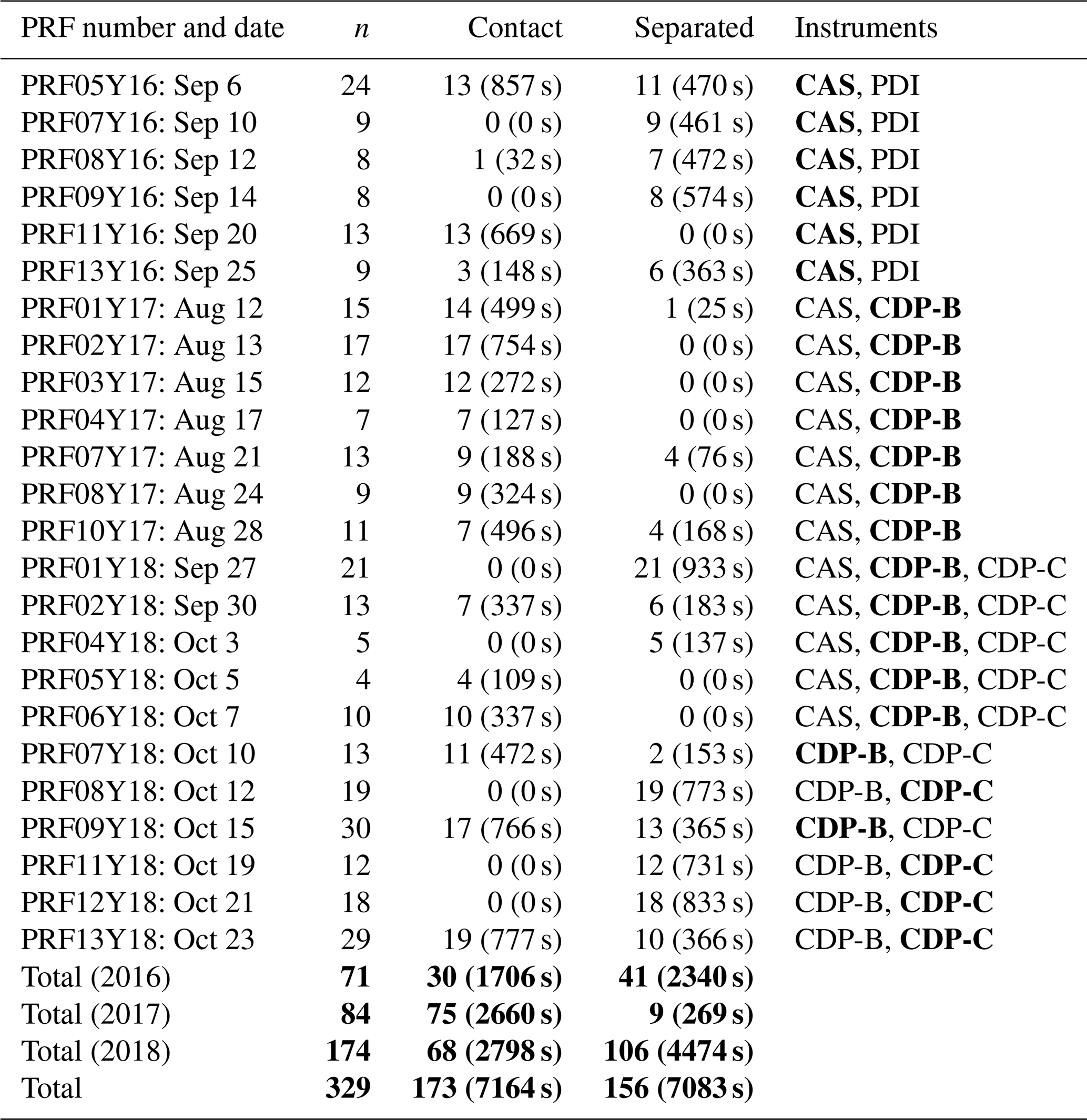
Figure 1 PRF tracks from ORACLES IOPs with base of operations and cloud sampling locations (tracks for multiple 2017 and 2018 PRFs overlap along 5^∘ E).

Three PRFs from the 2016 IOP had overlapping tracks when the P-3B aircraft flew northwest from 23^∘ S, 13.5^∘ E toward 10^∘ S, 0^∘ E and returned along the same track (Fig. 1). The 2017 and 2018 IOPs had 10 PRFs with overlapping flight tracks when the aircraft flew south from 0^∘ N, 5^∘ E toward 15^∘ S, 5^∘ E and returned along the same track. PRFs with overlapping tracks acquired statistics for model evaluation (Doherty et al., 2022), while the other PRFs targeted specific locations based on meteorological conditions (Redemann et al., 2021).

During ORACLES, the NASA P-3B aircraft was equipped with in situ probes. The data analyzed in this study were collected using Cloud Droplet Probes (CDPs) (Lance et al., 2010), a cloud and aerosol spectrometer (CAS) on the cloud, aerosol and precipitation spectrometer (Baumgardner et al., 2001), a phase Doppler interferometer (PDI) (Chuang et al., 2008), a two-dimensional stereo probe (2D-S) (Lawson et al., 2006), a high-volume precipitation sampler (HVPS-3) (Lawson et al., 1998), a King hot wire (King et al., 1978), and a Passive Cavity Aerosol Spectrometer Probe (PCASP) (Cai et al., 2013). A single CDP was used during the 2016 IOP (hereafter CDP-A), a second CDP (hereafter CDP-B) was added for the 2017 and 2018 IOPs, and CDP-A was replaced by a different CDP (hereafter CDP-C) for the 2018 IOP.

The CAS, CDP, King hot wire, and PCASP data were processed at the University of North Dakota using the Airborne Data Processing and Analysis processing package (Delene, 2011). The PDI data were processed at the University of Hawaii. The 2D-S and HVPS-3 data were processed using the University of Illinois/Oklahoma Optical Array Probe Processing Software (McFarquhar et al., 2018). The data processing procedures followed to reject artifacts were summarized by G21. Comparisons between the cloud probe datasets are described in the Supplement.

The King hot wire was used to sample LWC (hereafter King LWC). The PCASP was used to sample the accumulation-mode aerosols sized from 0.1 to 3.0 µm. The CAS, CDP, PDI, 2D-S, and HVPS-3 collectively sampled the number distribution function N(D) for particles with diameter D from 0.5 to 19200 µm. The size distribution covering the complete droplet size range was determined by merging the N(D) for 3<D<50 µm with the N(D) for 50<D<1050 µm from the 2D-S and the N(D) for 1050<D<19 200 µm from the HVPS-3. The HVPS-3 sampled droplets with D>1050 µm for a single 1 Hz data sample across the PRFs analyzed in this study. Measurement uncertainties in droplet sizes were expected to be within 20 % for droplets with D>5 µm from the CAS and the CDP, D>50 µm from the 2D-S, and D>750 µm from the HVPS-3 (Baumgardner et al., 2017).

During each PRF, at least two independent measurements of N(D) were made for 3<D<50 µm using the CAS, the PDI, or a CDP (Table 1). The differences between the N_c and LWC derived from the CAS, PDI, and CDP N(D) were quantified to determine if these differences were within measurement uncertainties. The LWC estimates from the CAS, PDI, and CDP were compared with the adiabatic LWC (LWC_ad), which represents the theoretical maximum for LWC (Brenguier et al., 2000). The N(D) for droplets with D<50 µm was determined using the probe which consistently had the LWC with better agreement with the LWC_ad during each IOP (see Supplement). LWC_ad can be used to compare LWC from different probes since it is derived using environmental conditions and does not depend on the cloud probe datasets. The relative differences between the LWC_ad and the LWC estimates from cloud probes provide a measure of the uncertainty associated with using one probe over the other for data analysis.

The differences between in-cloud datasets from different instruments were determined using a two-sample t test. The 95 % confidence intervals (CIs) between parameter means were reported if the differences were statistically significant. During the 2017 IOP, the CAS and the CDP-B sampled droplets with D<50 µm. The CDP-B LWC was higher than the CAS LWC (95 % CIs: 0.11 to 0.12 g m⁻³ higher), and the average CDP-B LWC (0.18 g m⁻³) had better agreement with the average LWC_ad (0.24 g m⁻³) compared to the average CAS LWC (0.08 g m⁻³). Thus, the CDP-B N(D) was used to represent the N(D) for droplets with D<50 µm for the 2017 IOP.

Similar results were obtained when the CAS LWC and the CDP-B LWC were compared with the LWC_ad for the 2018 IOP. During the 2018 IOP, the CDP-C was mounted at a different location relative to the aircraft wing compared to the CAS and CDP-B, and the positions of CDP-B and CDP-C were switched after 10 October 2018. O'Brien et al. (2022) found the CDP mounting positions had only a 6 % impact on the calculation of N_c, and the average CDP-B LWC and CDP-C LWC were within 0.02 g m⁻³. To maintain consistency with the 2017 IOP, data from the CDP mounted next to the CAS were used for droplets with D<50 µm for the 2018 IOP (except on 15 October 2018 when the CDP-C had a voltage issue).

During the 2016 IOP, measurements from the CDP-A were unusable for all PRFs due to an optical misalignment issue. Nevertheless, the CAS and the PDI sampled droplets with 3<D<50 µm. On average, the PDI LWC was higher than the CAS LWC (95 % CIs: 0.20 to 0.21 g m⁻³ higher). Since the PDI LWC was greater than the LWC_ad (95 % CIs: 0.04 to 0.06 g m⁻³ higher), it was hypothesized that the PDI LWC was an overestimate of the actual LWC. Thus, the CAS N(D) was used to represent the N(D) for droplets with D<50 µm for the 2016 IOP.

The 2D-S has two channels which concurrently sample the cloud volume. N_c and LWC were derived using data from the horizontal channel (N_H and LWC_H) and the vertical channel (N_V and LWC_V). N_H and LWC_H were used for the 2016 IOP because N_V and LWC_V were not available due to soot deposition on the inside of the receive-side mirror of the vertical channel. N_H and N_V as well as LWC_H and LWC_V were strongly correlated for the 2017 and 2018 IOPs, with Pearson's correlation coefficient R≥0.92 and the best-fit slope ≥0.90. The high correlation values suggest that little difference would have resulted from using the average of the two 2D-S channels. To maintain consistency with the 2016 IOP, N_H and LWC_H were used for all three IOPs.

3 Cloud properties

The N(D) from the merged droplet size distribution was integrated to calculate N_c. The 1 Hz data samples with N_c>10 cm⁻³ and King LWC >0.05 g m⁻³ were defined as in-cloud measurements (G21). The PCASP N(D) was used to determine the out-of-cloud N_a. In situ cloud sampling during ORACLES included flight legs when the P-3B aircraft ascended or descended through the cloud layer (hereafter cloud profiles). Data from 329 cloud profiles with just under 4 h of cloud sampling were examined (Table 1).

For every cloud profile, the cloud top height (Z_T) was defined as the highest altitude with N_c>10 cm⁻³ and King LWC >0.05 g m⁻³ (Table 2). The average Z_T during ORACLES was 1038±270 m, where the uncertainty estimate refers to the standard deviation. The cloud base height (Z_B) was defined as the lowest altitude with N_c>10 cm⁻³ and King LWC >0.05 g m⁻³. In decoupled boundary layers, a layer of cumulus can be present below the stratocumulus layer with a gap between the cloud layers (Wood, 2012). Measurements from stratocumulus were used in this study, and Z_B for the stratocumulus layer was identified as the altitude above which the King LWC increased without gaps greater than 25 m in the cloud sampling up to Z_T.

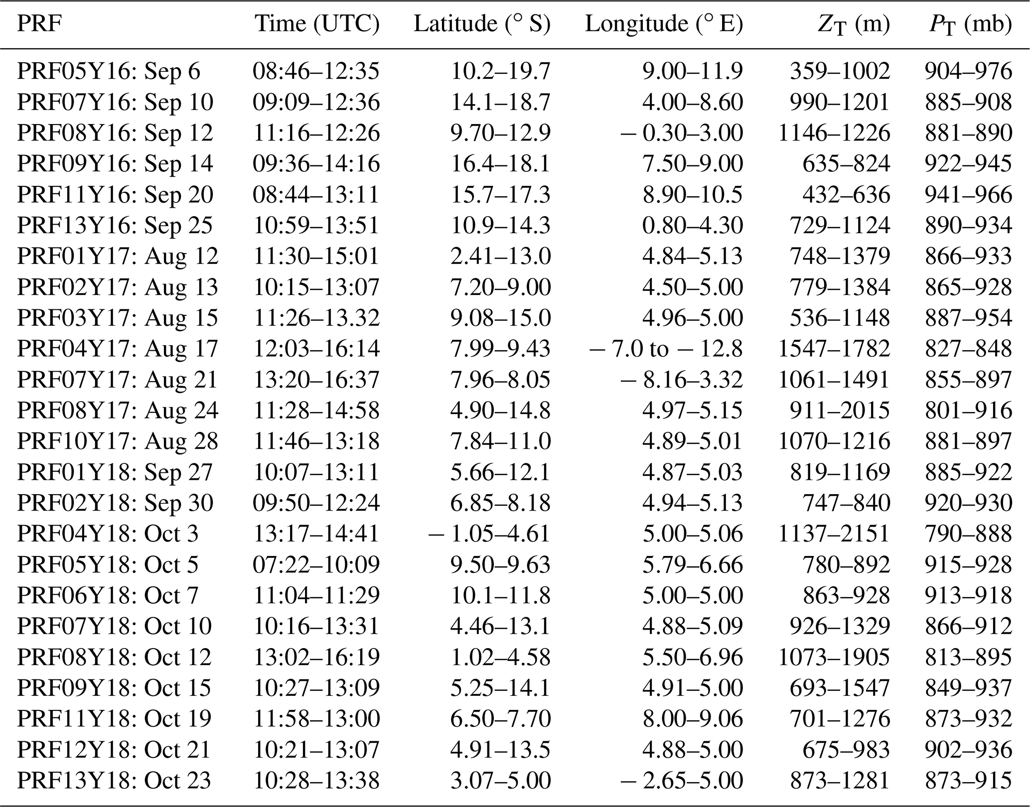
Table 2 Range of time, latitude, longitude, Z_T, and cloud top pressure (P_T) for PRFs in Table 1.

The difference between Z_T and Z_B was defined as H. Due to aerosol-induced changes in entrainment and boundary layer stability, the aerosol impact on H and Z_T can have the strongest influence on LWP adjustments associated with ACIs (Toll et al., 2019). Thus, the influence of ACIs on precipitation formation and S_o was examined as a function of H. Data collected during incomplete profiles of the stratocumulus or while sampling open-cell clouds (for example, on 2 October 2018) were excluded because of difficulties with estimating H for such profiles.

For each 1 Hz in-cloud data sample, the droplet size distribution was used to calculate R_e following Hansen and Travis (1974), where

$$\begin{array}{}\text{(1)}& R_{\mathrm{e}}\left(h\right)=\underset{\mathrm{3}}{\overset{\mathrm{\infty }}{\int }}{D}^{\mathrm{3}}N\left(D,h\right)\mathrm{d}D/\underset{\mathrm{3}}{\overset{\mathrm{\infty }}{\int }}\mathrm{2}{D}^{\mathrm{2}}N\left(D,h\right)\mathrm{d}D.\end{array}$$

Based on the aircraft speed, 1 Hz data samples corresponded to roughly 5 m intervals in the vertical direction. LWC was calculated as

$$\begin{array}{}\text{(2)}& \mathrm{LWC}\left(h\right)=\mathit{\pi }{\mathit{\rho }}_w/\mathrm{6}\underset{\mathrm{3}}{\overset{\mathrm{\infty }}{\int }}{D}^{\mathrm{3}}N\left(D,h\right)\mathrm{d}D,\end{array}$$

where ρ_w is the density of liquid water, and h is height in cloud above cloud base. LWC and King LWC were integrated over h from Z_B to Z_T to calculate LWP and King LWP, respectively. τ was calculated as

$$\begin{array}{}\text{(3)}& \begin{array}{rl}& {\mathit{\beta }}_{\mathrm{ext}}\left(h\right)=\underset{\mathrm{3}}{\overset{\mathrm{\infty }}{\int }}{Q}_{\mathrm{ext}}\mathit{\pi }/\mathrm{4}{D}^{\mathrm{2}}N\left(D,h\right)\mathrm{d}D,\\ & \mathit{\tau }=\underset{Z_{\mathrm{B}}}{\overset{Z_{\mathrm{T}}}{\int }}{\mathit{\beta }}_{\mathrm{ext}}\left(h\right)\mathrm{d}h,\end{array}\end{array}$$

where β_ext is the cloud extinction, and Q_ext is the extinction coefficient (approximately 2 for cloud droplets, assuming geometric optics apply for visible wavelengths) (Hansen and Travis, 1974). The integrals in Eqs. (1) to (3) were converted to discrete sums for D>3 µm to consider the contributions of cloud drops and not aerosols.

According to the adiabatic model (Brenguier et al., 2000), LWC_ad and LWP_ad are functions of H (the subscript “ad” added to represent the adiabatic equivalents). These relationships help parameterize τ_ad as

$$\begin{array}{}\text{(4)}& {\mathrm{LWC}}_{\mathrm{ad}}\left(h\right)\propto h,{\mathrm{LWP}}_{\mathrm{ad}}\propto H^{\mathrm{2}},{\mathit{\tau }}_{\mathrm{ad}}\propto (N_{\mathrm{c}}{)}^{\mathrm{1}/\mathrm{3}}{\mathrm{LWP}}^{\mathrm{5}/\mathrm{6}}.\end{array}$$

4 Aerosol influence on cloud microphysics

The MSCs over the Southeast Atlantic were overlaid by biomass burning aerosols from southern Africa (Adebiyi and Zuidema, 2016; Redemann et al., 2021), with instances of contact and separation between the MSC cloud tops and the base of the biomass burning aerosol layer (G21). Across the three IOPs, 173 profiles were conducted at locations where an extensive aerosol plume with N_a>500 cm⁻³ was located within 100 m above Z_T (hereafter contact profiles) (Table 1). 156 profiles were conducted at locations where the level of N_a>500 cm⁻³ was located at least 100 m above Z_T (hereafter separated profiles). About 50 % of the in situ cloud sampling across the three IOPs was conducted during contact profiles (Table 1). Due to inter-annual variability, contact profiles accounted for about 42 %, 91 %, and 39 % of the in situ cloud sampling during the 2016, 2017, and 2018 IOPs, respectively.

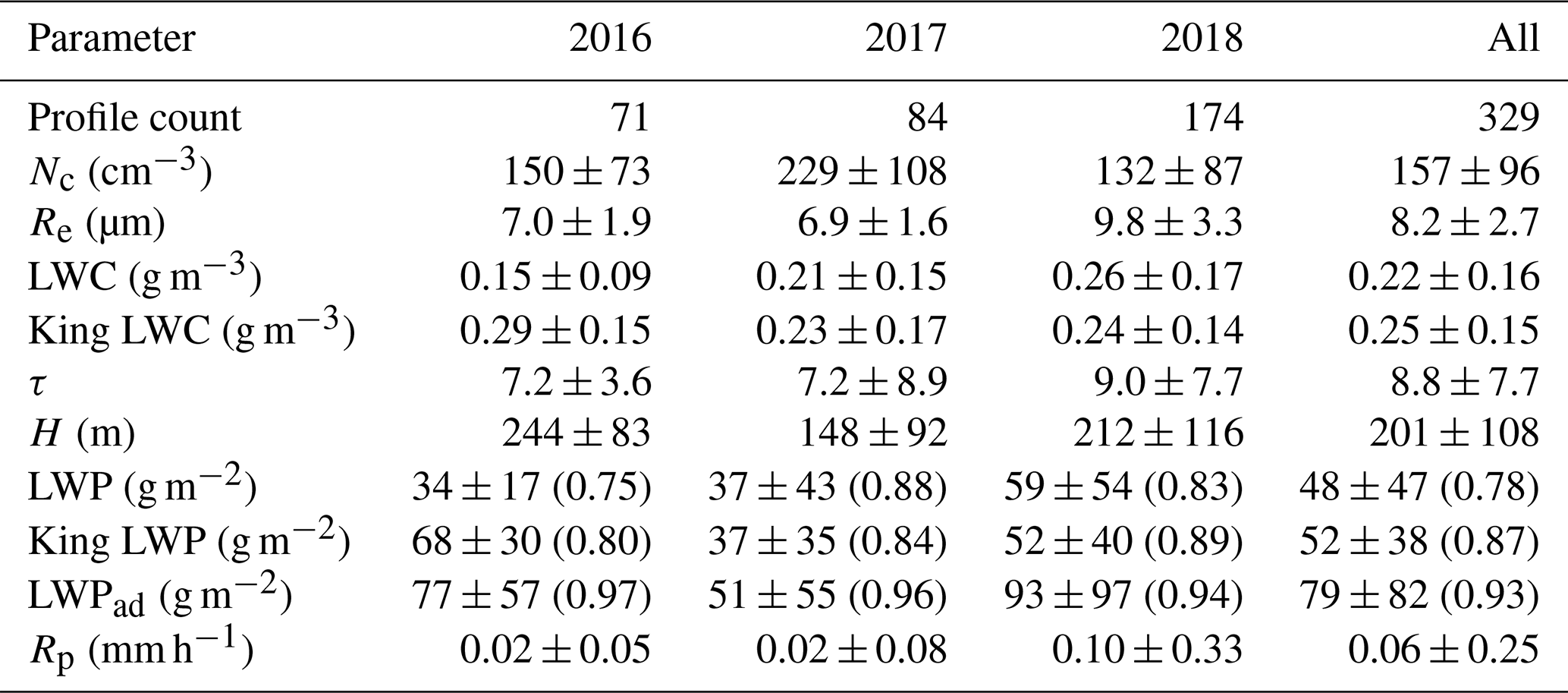
The average N_c and R_e for all cloud profiles across the three IOPs were 157±96 cm⁻³ and 8.2±2.7 µm, respectively (Table 3). The high proportion of contact profiles during the 2017 IOP was associated with higher average N_c and lower average R_e (229 cm⁻³ and 6.9 µm) compared to the 2016 IOP (150 cm⁻³ and 7.0 µm) and the 2018 IOP (132 cm⁻³ and 9.8 µm). It is possible that the use of CDP-B data for the 2017 IOP contributed to the increase in average N_c relative to the 2016 IOP. However, the difference between the average CAS N_c and the average CDP-B N_c for the 2017 IOP (12 cm⁻³) was lower than the difference between the average N_c for the 2016 and 2017 IOPs (79 cm⁻³). The difference between the N_c for these IOPs was thus primarily due to the conditions at the cloud sampling locations. The microphysical differences between the 2016 and 2017 IOPs were associated with differences in surface precipitation. Based on the W-band retrievals from the Jet Propulsion Laboratory Airborne Precipitation Radar Version 3 (APR-3), the 2017 IOP had fewer profiles with precipitation reaching the surface (13 %) compared to the 2016 IOP (34 %) (Dzambo et al., 2019).

Table 3 Average values for cloud properties measured during cloud profiles from the PRFs listed in Table 1 for each IOP. Error estimates represent 1 standard deviation. R between LWP estimates and H in parentheses.

On average, contact profiles had significantly higher N_c (95 % CIs: 84 to 90 cm⁻³ higher) and lower R_e (95 % CIs: 1.4 to 1.6 µm lower) compared to separated profiles (throughout the study, the term “significant” is exclusively used to represent statistical significance). The significant differences in N_c and R_e were associated with significantly higher τ (95 % CIs: 0.04 to 3.06 higher) for contact profiles, in accordance with the Twomey effect (Twomey, 1974, 1977). These results were consistent with the 2016 IOP when the contact profiles had higher N_c (95 % CIs: 60 to 68 cm⁻³ higher), lower R_e (95 % CIs: 1.1 to 1.3 µm lower), and higher τ (95 % CIs: 1.1 to 4.3 higher) (G21).

Figure 2 shows violin plots for cloud properties as a function of normalized height (Z_N), defined as $Z_{\mathrm{N}}=Z--Z_{\mathrm{B}}/Z_{\mathrm{T}}-Z_{\mathrm{B}}$. The violin plots include box plots and illustrate the distribution of the data (Hintze and Nelson, 1998). The median N_c increased with Z_N for Z_N≤0.25, consistent with droplet nucleation (Fig. 2a). The median N_c decreased near cloud top for Z_N≥0.75 from 204 to 154 cm⁻³ for contact and from 104 to 69 cm⁻³ for separated profiles. This is consistent with droplet evaporation associated with cloud-top entrainment (G21). The median R_e increased with Z_N consistent with condensational growth (Fig. 2b). There was a greater increase in the median R_e from cloud base to cloud top for separated profiles (from 7.1 to 9.5 µm) compared to contact profiles (from 6.1 to 7.9 µm). This is consistent with previous observations of stronger droplet growth in cleaner conditions as a function of Z_N (Braun et al., 2018; G21) and LWP (Rao et al., 2020). Statistically insignificant differences between the average H for contact and separated profiles suggest that the differential droplet growth was associated with differences in cloud processes like collision–coalescence (further discussed in Sect. 5).

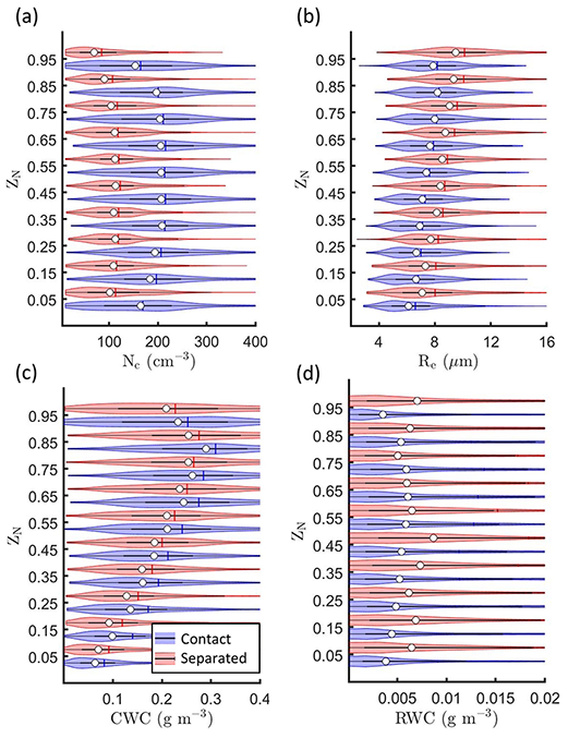
Figure 2 Kernel density estimates (distribution of the data indicated by width of shaded area) and box plots showing the 25th, 50th (white circle), and 75th percentiles for (a) N_c, (b) R_e, (c) CWC, and (d) RWC as a function of Z_N for contact and separated profiles.

The LWC and LWP responses to changes in aerosol conditions were examined because the adiabatic model suggests $\mathit{\tau }\mathit{\alpha }{\mathrm{LWP}}^{\mathrm{5}/\mathrm{6}}$ (Eq. 4) (Brenguier et al., 2000). Contact profiles had significantly higher LWC, but the relative increase was less than 10 % (Table 4). LWC was divided into rainwater content (RWC) and cloud water content (CWC) based on droplet size. Droplets with D>50 µm were defined as drizzle (Abel and Boutle, 2012; Boutle et al., 2014), and the total drizzle mass was defined as RWC. The droplet mass for D<50 µm was defined as CWC. Rainwater path (RWP) and (cloud water path) CWP were defined as the vertical integrals of RWC and CWC, respectively. The median CWC increased with Z_N but decreased over the top 10 % of the cloud layer for contact profiles and over the top 20 % of the cloud layer for separated profiles, consistent with cloud-top entrainment (Fig. 2c). For contact profiles, the median RWC increased with Z_N before decreasing for Z_N≥0.75. The median RWC for separated profiles varied with Z_N. The bottom half of the cloud layer had higher median values (up to $\mathrm{8.7}\times {\mathrm{10}}^{-\mathrm{3}}$ g m⁻³) compared to the top half (up to $\mathrm{7.0}\times {\mathrm{10}}^{-\mathrm{3}}$ g m⁻³) (Fig. 2d).

Table 4 Average and standard deviation for cloud properties measured during contact and separated profiles with 95 % confidence intervals (CIs) from a two-sample t test applied to contact and separated profile data. Positive CIs indicate higher average for contact profiles, and “insignificant” indicates statistically similar averages for contact and separated profiles.

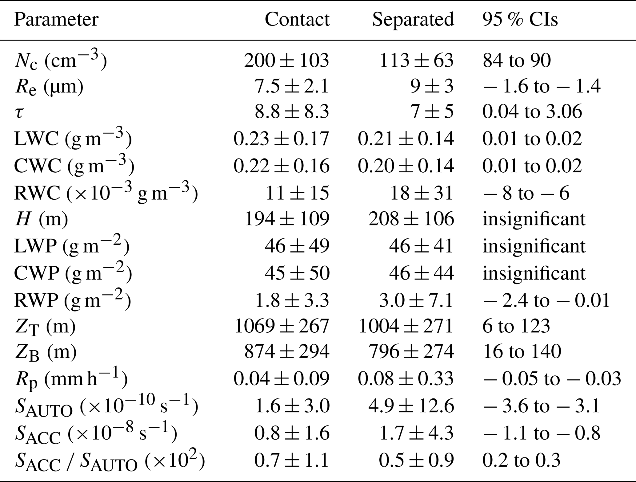
For contact profiles, there was a significant increase in the average CWC (10 %) and a significant decrease in the average RWC (60 %) compared to separated profiles (Table 4). Contact profiles also had significantly lower average RWP with insignificant differences for average CWP (Table 4). Contact profiles were located in deeper boundary layers with significantly higher Z_B and Z_T compared to separated profiles. However, the decrease in RWC cannot be attributed to differences in H or LWP (Kubar et al., 2009) because of statistically similar H and LWP for contact and separated profiles, on average (Table 4). These results show that instances of contact between above-cloud aerosols and the MSC were associated with more numerous and smaller cloud droplets and weaker droplet growth compared to instances of separation between the above-cloud aerosols and the MSC.

5 Precipitation formation and H

The precipitation rate R_p was calculated using the drizzle water content and fall velocity u(D) following Abel and Boutle (2012):

$$\begin{array}{}\text{(5)}& R_{\mathrm{p}}=\mathit{\pi }/\mathrm{6}\underset{\mathrm{50}\mathrm{\mu }m}{\overset{\mathrm{\infty }}{\int }}n\left(D\right)D^{\mathrm{3}}u\left(D\right)\mathrm{d}D,\end{array}$$

with fall velocity relationships from Rogers and Yau (1989) used in the computation.

Contact profiles had significantly lower R_p compared to separated profiles (95 % CIs: 0.03 to 0.05 mm h⁻¹ lower). This suggests contact between the MSC and above-cloud biomass burning aerosols was associated with precipitation suppression. LWP and H impact the sign and magnitude of the precipitation changes in response to changes in aerosol conditions (Kubar et al., 2009; Christensen and Stephens, 2012). Thus, cloud and precipitation properties were evaluated as a function of H to examine the aerosol-induced changes in precipitation formation.

The 95th percentile was used to represent the maximum value of a variable. For example, the 95th percentile of R_p (denoted by R_p95) represents the maximum R_p during a cloud profile. Although more numerous contact profiles were drizzling compared to separated profiles, the latter had more numerous profiles with high precipitation intensity. For instance, 114 out of 173 contact and 95 out of 156 separated profiles were drizzling with R_p95>0.01 mm h⁻¹, out of which 36 contact and 40 separated profiles had R_p95>0.1 mm h⁻¹, and only 1 contact and 9 separated profiles had R_p95>1 mm h⁻¹ (Fig. 3a). This is consistent with radar retrievals of surface R_p<1 mm h⁻¹ for over 93 % of the radar profiles from 2016 and 2017 (Dzambo et al., 2019).

Figure 3 The 95th percentile for (a) R_p, (b) CWC, (c) N_c, and (d) R_e as a function of H. Each dot represents the 95th percentile from the 1 Hz measurements for a single cloud profile. Pearson's correlation coefficient (R) and p value for the correlation indicated in legend.

5.1 Microphysical properties

On average, separated profiles had greater R_p95 (0.22 mm h⁻¹) compared to contact profiles (0.07 mm h⁻¹). R_p95 was positively correlated with H as thicker profiles had higher precipitation intensity (Fig. 3a). The average R_p95 increased from thin (H<175 m) to thick clouds (H>175 m) from 0.04 to 0.10 mm h⁻¹ for contact and 0.13 to 0.29 mm h⁻¹ for separated profiles. Precipitation intensity thus decreased from separated to contact profiles for both thin and thick profiles. The average R_p95 for thin and thick contact profiles was 32 % and 37 % of the average R_p95 for thin and thick separated profiles, respectively.

CWC₉₅ was positively correlated with H as thicker clouds had higher droplet mass (Fig. 3b). This was consistent with condensational and collision–coalescence growth continuing to occur with greater height above cloud base (Fig. 2b, c) and greater cloud depth allowing for greater droplet growth. N_c95 and R_e95 were negatively and positively correlated with H, respectively (Fig. 3c, d). The trends in N_c and R_e versus H were consistent with the process of collision–coalescence resulting in fewer and larger droplets.

On average, contact profiles had higher N_c95 and lower R_e95 (311 cm⁻³ and 8.6 µm) compared to separated profiles (166 cm⁻³ and 10.8 µm). It can be inferred that the presence of more numerous and smaller droplets during contact profiles decreased the efficiency of collision–coalescence. Alternatively, there may not have been sufficient time for the updraft to produce the few large droplets needed to broaden the size distribution and initiate collision–coalescence. Since contact and separated profiles had statistically similar H (Table 4), the following discussion examines the link between precipitation suppression and the aerosol-induced changes in N_c, R_e, and LWC and their impact on precipitation.

5.2 Precipitation properties

Precipitation formation process rates were estimated using equations used in numerical models to compare precipitation formation between contact and separated profiles. Precipitation development in models is parameterized using bulk microphysical schemes. General circulation models (GCMs) or large eddy simulation (LES) models parameterize precipitation formation using S_AUTO and S_ACC (e.g., Penner et al., 2006; Morrison and Gettelman, 2008; Gordon et al., 2018). The most commonly used parameterizations were used to estimate equivalent rates of precipitation formation from models. S_AUTO and S_ACC were calculated following Khairoutdinov and Kogan (2000):

$$\begin{array}{}\text{(6)}& S_{\mathrm{AUTO}}={\left(\mathrm{d}{w}_{\mathrm{r}}\right)}_{\mathrm{AUTO}}/\mathrm{d}t=\mathrm{1350}{w}_{\mathrm{c}}^{\mathrm{2.47}}{N}_{\mathrm{c}}^{-\mathrm{1.79}}\end{array}$$

and

$$\begin{array}{}\text{(7)}& S_{\mathrm{ACC}}={\left(\mathrm{d}{w}_{\mathrm{r}}\right)}_{\mathrm{ACC}}/\mathrm{d}t=\mathrm{67}{\left(w_{\mathrm{c}}{w}_{\mathrm{r}}\right)}^{\mathrm{1.15}},\end{array}$$

where w_c and w_r are cloud water and rainwater mixing ratios, respectively, and are equal to the CWC and RWC divided by the density of air (ρ_a).

Contact profiles had significantly lower S_AUTO and S_ACC compared to separated profiles (Table 4). This is consistent with significantly lower RWC and R_p for contact profiles and the association of S_AUTO and S_ACC with precipitation onset and precipitation intensity, respectively. S_AUTO95 and S_ACC95 were positively correlated with H (Fig. 4a, b). Separated profiles had higher S_AUTO95 and S_ACC95 ($\mathrm{9.6}\times {\mathrm{10}}^{-\mathrm{10}}$ and $\mathrm{2.2}\times {\mathrm{10}}^{-\mathrm{8}}$ s⁻¹) compared to contact profiles ($\mathrm{2.9}\times {\mathrm{10}}^{-\mathrm{10}}$ and $\mathrm{1.2}\times {\mathrm{10}}^{-\mathrm{8}}$ s⁻¹), associated with the inverse relationship between S_AUTO and N_c (Eq. 6). Faster autoconversion resulted in higher drizzle water content and greater accretion of droplets on drizzle drops.

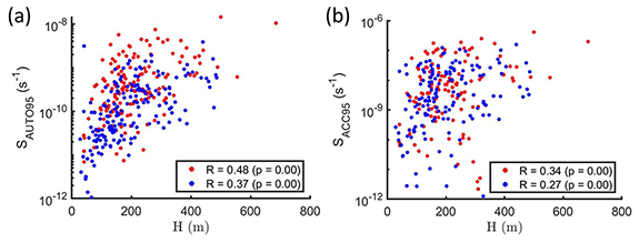
Figure 4 The 95th percentile for (a) S_AUTO and (b) S_ACC as a function of H. Each dot represents the 95th percentile from the 1 Hz measurements for a single cloud profile. R and p value for the correlation indicated in legend.

The sampling of lower N_c95 and higher R_e95 compared to thinner profiles suggests that collision–coalescence was more effective in profiles with higher H (Fig. 3c, d). Thin contact profiles had the lowest S_AUTO95 ($\mathrm{1.4}\times {\mathrm{10}}^{-\mathrm{10}}$ s⁻¹), followed by thick contact ($\mathrm{4.5}\times {\mathrm{10}}^{-\mathrm{10}}$ s⁻¹), thin separated ($\mathrm{4.7}\times {\mathrm{10}}^{-\mathrm{10}}$ s⁻¹), and thick separated profiles ($\mathrm{1.4}\times {\mathrm{10}}^{-\mathrm{9}}$ s⁻¹). High N_c and low CWC for thin contact profiles (Fig. 3b, c) are consistent with increased competition for cloud water leading to weaker autoconversion. It is hypothesized that these microphysical differences resulted in the lower S_AUTO95 and R_p95 for thin contact profiles compared to other profiles. The differences between R_p for contact and separated profiles thus varied with H in addition to N_c, R_e, and CWC. N_c, R_e, and CWC varied with N_a (Sect. 4), and ACIs were examined in Sects. 6 and 7.

6 Aerosol influence on precipitation

6.1 Below-cloud N_a

Polluted boundary layers in the Southeast Atlantic are associated with entrainment mixing between the free troposphere and the boundary layer (Diamond et al., 2018). Ground-based observations from Ascension Island have shown clean boundary layers can have elevated biomass burning trace gas concentrations during the burning season (Pennypacker et al., 2020). This suggests boundary layers could be clean in terms of N_a despite the entrainment of biomass burning aerosols into the boundary layer due to precipitation scavenging of below-cloud aerosols. Carbon monoxide (CO) concentrations were examined since CO acts as a biomass burning tracer that is unaffected by precipitation scavenging (Pennypacker et al., 2020). For the 2016 IOP, contact profiles were located in boundary layers with significantly higher N_a (95 % CIs: 93 to 115 cm⁻³ higher) and CO (95 % CIs: 13 to 16 ppb higher) compared to separated profiles (G21). This is consistent with data from all three IOPs when contact profiles were located in boundary layers with higher N_a (95 % CIs: 231 to 249 cm⁻³ higher) and CO (95 % CIs: 27 to 29 ppb higher).

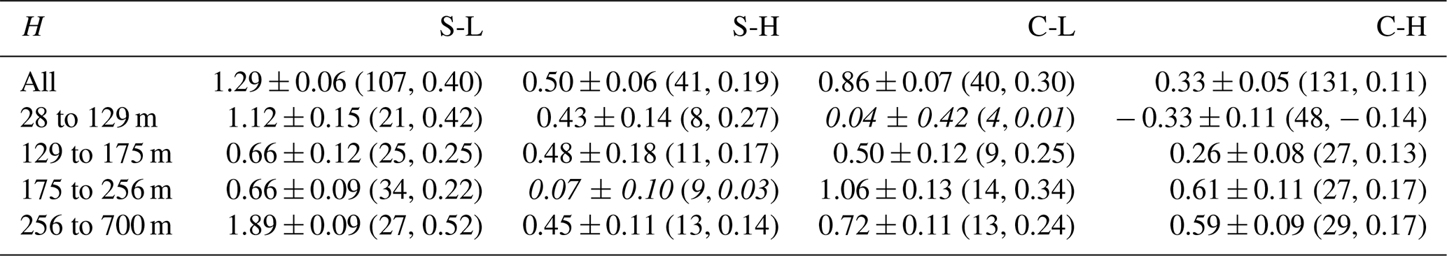
Following G21, 171 contact and 148 separated profiles from the IOPs were classified into four regimes: contact, high N_a (C-H); contact, low N_a (C-L); separated, high N_a (S-H); and separated, low N_a (S-L), where “low N_a” meant the profile was in a boundary layer with N_a<350 cm⁻³ up to 100 m below cloud base. Boundary layer CO concentration above 100 ppb was sampled during 107 contact and 31 separated profiles, respectively. Contact profiles were more often located in high N_a boundary layers (131 out of 171 profiles classified as C-H), while separated profiles were more often located in low N_a boundary layers (108 out of 148 profiles classified as S-L). This suggests contact between MSC cloud tops and above-cloud biomass burning aerosols was associated with the entrainment of biomass burning aerosols into the boundary layer.

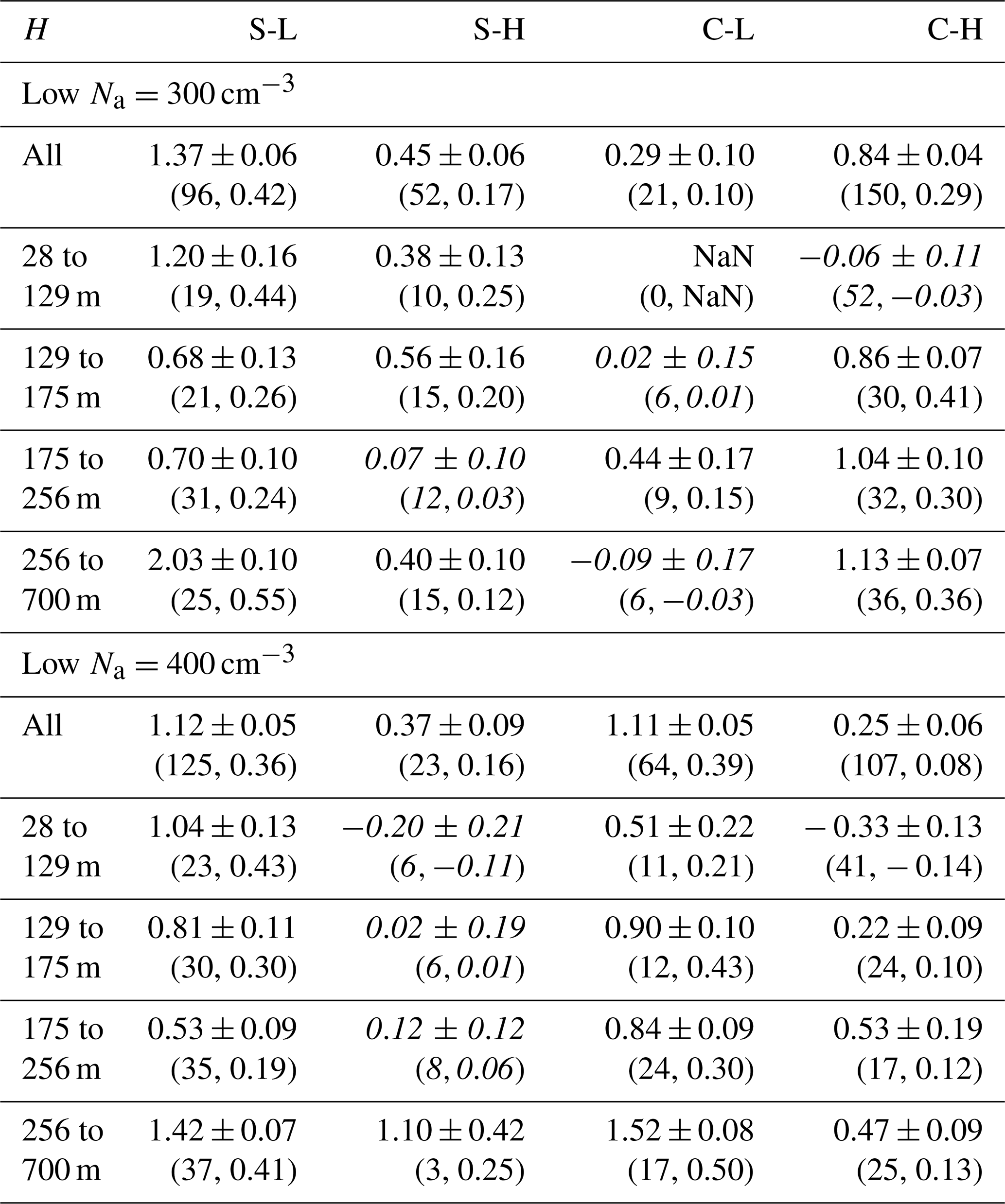
Contact profiles had significantly higher N_c and significantly lower R_e relative to separated profiles in both high N_a (C-H relative to S-H) and low N_a (C-L relative to S-L) boundary layers (Fig. 5, Table 5). This was associated with significantly higher above- and below-cloud N_a for the contact profiles. The differences in N_c and R_e were higher in high N_a boundary layers, where the differences in above- and below-cloud N_a were also higher compared to low N_a boundary layers (Table 5). This is consistent with previous observations of MSC properties (Diamond et al., 2018; Mardi et al., 2019) and similar analysis for data from the 2016 IOP (G21).

Table 5 Average values for aerosol and cloud properties from C-H, S-H, C-L, and S-L regimes (defined in text), along with differences reported as 95 % CIs.

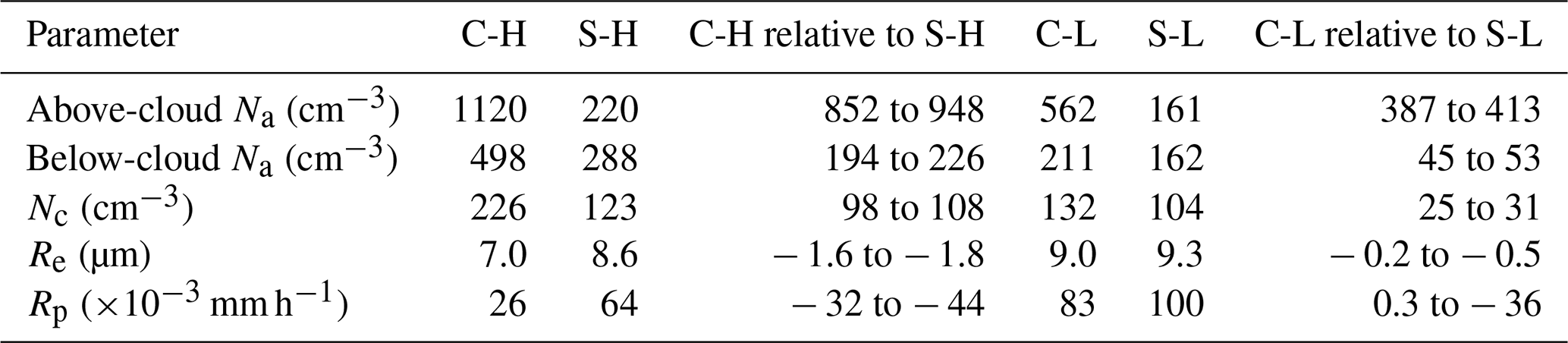
Figure 5 Average N_c (error bars extend to 95 % CIs) as a function of Z_N. Number of 1 Hz data points and corresponding regimes indicated in legend.

C-L profiles had significantly higher N_c (95 % CIs: 5 to 14 cm⁻³ higher) compared to S-H profiles, despite having significantly lower below-cloud N_a (95 % CIs: 69 to 85 cm⁻³ lower). Significantly higher above-cloud N_a for C-L profiles (95 % CIs: 321 to 361 cm⁻³ higher) suggests that this was associated with the influence of above-cloud N_a on N_c. However, the smaller difference in N_c compared to the differences between C-H and S-H or C-L and S-L profiles suggests the combined impact of above- and below-cloud N_a was stronger than the impact of above-cloud N_a alone. These comparisons were qualitatively consistent when thresholds of 300 or 400 cm⁻³ were used to define a low N_a boundary layer.

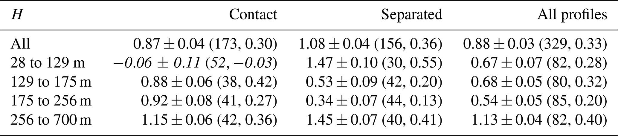
Table 6 S_o ± standard error for contact, separated, and all profiles, with sample size and R in parentheses. The use of italics denotes the statistical insignificance of S_o.

6.2 N_c and R_p versus H

The cloud profiles were divided into four populations based on H to compare N_c and R_p between different aerosols conditions, while H was constrained. The populations were divided at H=129, 175, and 256 m to ensure similar sample sizes (Table 6). For each population, contact profiles had higher N_c and lower R_p (Fig. 6a, b), consistent with comparisons averaged over all profiles (Table 4). Due to collision–coalescence, the average N_c decreased, and the average R_p increased with H (Fig. 6a, b). For contact profiles, the average N_c decreased with H from 221 to 191 cm⁻³, and the average R_p increased from 0.03 to 0.07 mm h⁻¹. For separated profiles, the average N_c decreased from 149 to 92 cm⁻³, and the average R_p increased from 0.06 to 0.21 mm h⁻¹ over the same range of H. C-H profiles had the highest average N_c and the lowest average R_p among the four regimes due to high above- and below-cloud N_a (Fig. 6c, d). C-H profiles had the smallest increase in the average R_p with H (0.02 to 0.04 mm h⁻¹). Conversely, low above- and below-cloud N_a for S-L profiles was associated with the lowest average N_c, the highest average R_p, and the highest increase in the average R_p with H (0.12 to 0.29 mm h⁻¹). For each regime, the average N_c decreased with H (except C-L), and the average R_p increased with H (Fig. 6c, d).

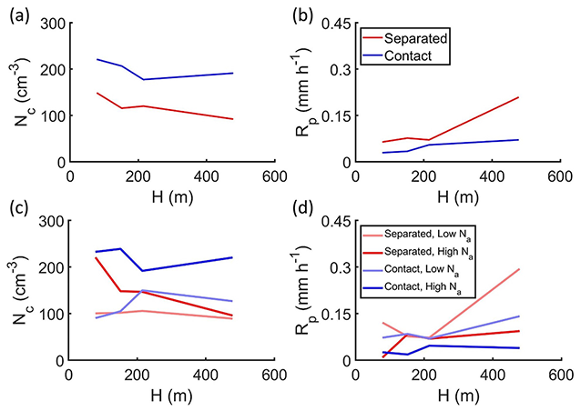
Figure 6 The average (a, c) N_c and (b, d) R_p as a function of H for (a, b) contact and separated profiles and (c, d) the regimes indicated in legend.

6.3 Precipitation susceptibility S_o

S_o was used to evaluate the dependence of R_p on N_c under the different aerosol conditions. S_o, defined as the negative slope between the natural logarithms of R_p and N_c (Feingold and Seibert, 2009), is given by

$$\begin{array}{}\text{(8)}& S_{\mathrm{o}}=-\mathrm{d}\ln \left(R_{\mathrm{p}}\right)/\mathrm{d}\ln \left(N_{\mathrm{c}}\right),\end{array}$$

where a positive value indicates decreasing R_p with increasing N_c, in accordance with the “lifetime effect” (Albrecht, 1989). The average S_o across all profiles was 0.88±0.03, with lower S_o for contact profiles (0.87±0.04) compared to separated profiles (1.08±0.04) (Table 6). This is consistent with the hypothesis of lower values for S_o analogues (where N_c in Eq. (8) is replaced by N_a) in the presence of above-cloud aerosols (Duong et al., 2011). S_o depends on the ratio of S_ACC to S_AUTO because S_ACC is independent of N_c, and higher $S_{\mathrm{ACC}}/S_{\mathrm{AUTO}}$ represents weaker dependence of R_p on N_c (Wood et al., 2009; Jiang et al., 2010). Lower S_o for contact profiles was associated with higher $S_{\mathrm{ACC}}/S_{\mathrm{AUTO}}$ compared to separated profiles (Table 4).

S_o was calculated as a function of H using N_c and R_p for the four populations of cloud profiles (Fig. 7). The sensitivity of S_o to the number of populations is discussed in Appendix A. Averaged over all profiles, S_o had minor variations with H (e.g., 0.67, 0.68, and 0.54 as H increased) before increasing to 1.13 for H>256 m (Table 6). This trend in S_o versus H is consistent with previous analyses of S_o (Sorooshian et al., 2009; Jung et al., 2016). However, different trends emerged when S_o was calculated for contact and separated profiles.

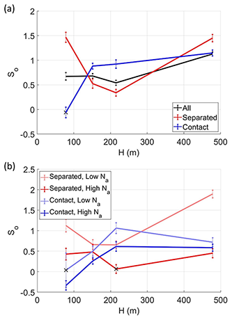
Figure 7 S_o as a function of H (error bars extend to standard error from the regression model) for (a) contact, separated, and all profiles and (b) the regimes indicated in legend. S_o was statistically insignificant when marked with a cross.

The largest difference between S_o for contact and separated profiles was observed for thin clouds with H<129 m. The 30 separated profiles with H<129 m had the highest S_o (1.47±0.10) because of strong dependence of R_p on N_c. For these profiles, measurements with low N_c (<100 cm⁻³) had higher R_p (0.18 mm h⁻¹) compared to measurements with higher N_c (0.01 mm h⁻¹) (Fig.  8a). In contrast, the 52 contact profiles with H<129 m had a low and statistically insignificant value for S_o ($-\mathrm{0.06}\pm \mathrm{0.11}$) due to poor (and statistically insignificant) correlation ($R=-\mathrm{0.03}$). Poor correlation between N_c and R_p for contact profiles was associated with precipitation suppression and weaker droplet growth (Sect. 5). These factors resulted in R_p<0.03 mm h⁻¹ independent of the N_c measurement (Fig. 8a).

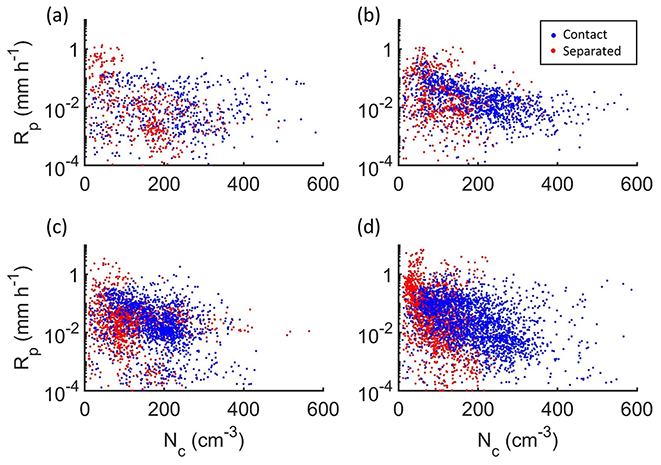
Figure 8 Scatter plots of R_p and N_c for 1 Hz data points from contact and separated profiles with (a) 28<H<129 m, (b) 129<H<175 m, (c) 175<H<256 m, and (d) 256<H<700 m.

For separated profiles, S_o decreased with H from 1.47±0.10 for H<129 m to 0.53±0.09 for 129<H<175 m and to 0.34±0.07 for 175<H<256 m (Fig. 7a). This was due to the increase in average R_p for high N_c measurements as a function of H from 0.01 mm h⁻¹ to 0.05 and 0.04 mm h⁻¹, respectively. R_p increased with H due to stronger collision–coalescence as droplet mass increased with H. Separated profiles with H>256 m had lower N_c and higher R_p compared to the populations with lower H (Fig. 6a, b). For measurements with low N_c, collision–coalescence and stronger autoconversion (following Eq. 6) resulted in higher R_p (0.26 mm h⁻¹) compared to measurements with higher N_c (0.13 mm h⁻¹). This led to a strong gradient R_p as a function of N_c (Fig. 8d), and S_o increased to 1.45±0.07 for separated profiles with H>256 m.

For contact profiles with H>129 m, the average R_p increased with H, with a larger increase for measurements with low N_c (0.028 to 0.12 mm h⁻¹) compared to measurements with high N_c (0.03 to 0.06 mm h⁻¹). It is hypothesized that collision–coalescence was hindered by the presence of more numerous droplets for the latter. With droplet growth and collision–coalescence for higher H, the limiting factor for R_p changed from H to N_c. The dependence of R_p on N_c thus increased with H, and, as a result, S_o increased with H from 0.88±0.06 to 1.15±0.06 (Fig. 7a).

Among the four regimes defined based on the above- and below-cloud N_a, S-L profiles had the highest S_o (1.12) (Table 7). This was associated with S-L profiles having the lowest N_c and the highest R_p among the regimes (Fig. 6c, d). In descending order of S_o, S-L profiles were followed by C-L (0.86), S-H (0.50), and C-H profiles (0.33). Profiles in low N_a boundary layers (S-L and C-L) had higher S_o compared to profiles in high N_a boundary layers (S-H and C-H), consistent with wet scavenging of below-cloud aerosols (Duong et al., 2011; Jung et al., 2016).

Table 7 S_o ± standard error with sample size and R in parentheses for cloud regimes defined in text. The use of italics denotes the statistical insignificance of S_o.

C-L and C-H profiles had similar trends in S_o except for profiles with H<129 m (Fig. 7b). C-L profiles had an insignificant value for S_o due to low sample size (4), and C-H profiles had negative S_o. These were thin profiles with little cloud water (Fig. 4b), high N_c (Fig. 6c), and low R_p (Fig. 6d). It is hypothesized that increasing N_c would provide the cloud water required for precipitation initiation and aid collision–coalescence. A total of 107 out of 148 separated profiles were classified as S-L profiles. As a result, separated and S-L profiles had similar trends in S_o versus H (Fig. 7). On average, S-L profiles had higher S_o than S-H profiles, which could be associated with wet scavenging, resulting in the lower below-cloud N_a for S-L profiles. For S-H profiles, S_o was constant with H at about 0.45 (except 175<H<256 m when the value for S_o was insignificant).

The sensitivity of S_o to removal of clouds based on R_p was examined in Appendix B. The removal of clouds with low R_p and high N_c or with high R_p and low N_c resulted in lower average S_o consistent with previous work (Duong et al., 2011). The S_o comparisons between profiles located in high N_a or low N_a boundary layers varied with the sample sizes of the populations. The sample sizes varied based on the threshold used to define a low N_a boundary layer which is discussed in Appendix C. CAS data were used to represent measurements of droplets with D<50 µm collected during ORACLES 2016 in the absence of CDP data. The sensitivity of S_o to the use of CAS data was examined in Appendix D.

6.4 S_o discussion

Figure 9 shows how S_o varied with perturbations (Δ) in N_c or R_p. Previous studies hypothesized that increasing above-cloud N_a or precipitation scavenging of below-cloud N_a would lead to changes in S_o (Fig. 4, Duong et al., 2011; Fig. 11, Jung et al., 2016). Thus, ΔN_c and ΔR_p for clouds with variable above- and below-cloud N_a were quantified in this study (Table 5). Higher N_c and lower R_e for contact profiles led to precipitation suppression along with lower S_AUTO, S_ACC, and R_p, which were associated with lower S_o compared to separated profiles. As a result, polluted clouds were 20 % less susceptible to precipitation suppression than cleaner clouds. Figure 9 shows that the impact of ΔN_c or ΔR_p on S_o depends on the original values for N_c and R_p as the same ΔN_c and ΔR_p can have an opposing effect on S_o. For example, a decrease in N_c at point 1 would decrease the slope and the S_o value, while the same decrease in N_c at point 2 would increase the slope and the S_o value.

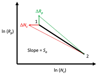
Figure 9 An illustration of the dependence of S_o on N_c, R_p, and perturbations (Δ) in N_c or R_p.

Both average and maximum N_c and R_p varied with H due to increasing aerosols (Sect. 4) and droplet growth due to collision–coalescence, autoconversion, and accretion (Sect. 5). Further, co-variability between droplet growth processes and ACIs meant aerosol-induced ΔN_c and ΔR_p varied with H (Sect. 6.2). Consequently, the differences between S_o for clean and polluted clouds varied with H. The change in S_o was highest for thin polluted clouds due to poor correlation between N_c and R_p as limited droplet growth led to low R_p regardless of the N_c. Future work must examine the co-variability between ΔN_c or ΔR_p from cloud processes such as droplet growth, entrainment, invigoration, precipitation, and ΔN_c or ΔR_p due to ACIs. Model parameterizations with power-law relationships between R_p, N_c, and H (Geoffroy et al., 2008) must account for changes in the dependence of R_p on $N_{\mathrm{c}}/H$ due to increasing aerosols or H.

The trends in S_o were only compared with studies analyzing airborne data due to the variability in S_o depending on whether aircraft, remote sensing, or modeling data were examined (Sorooshian et al., 2019). Consistent with Terai et al. (2012), S_o decreased with H for separated profiles with H<256 m. The results from Sect. 5 suggest droplet growth with H decreased the susceptibility to aerosols because R_p was limited by droplet growth instead of N_a or N_c. In comparison, S_o increased with H for contact profiles, consistent with Jung et al. (2016). The low S_o for thin contact profiles was consistent with the low S_o (0.06) for thin MSC over the southeast Pacific (Jung et al., 2016). This was attributed to insufficient cloud water for precipitation initiation (as noted in Sect. 5). An airborne investigation of marine stratocumulus off the Californian coast attributed negative values of S_o to the influence of giant cloud condensation nuclei (Dadashazar et al., 2017). The authors hypothesized that the low statistical significance of the negative estimate of S_o could be associated with precipitation suppression by aerosol particles.

Jung et al. (2016) analyzed MSC sampled farther east and away from South America compared to Terai et al. (2012). They argued a westward increase in precipitation frequency and intensity, along with a decrease in aerosols and N_c, led to the differences between the two studies. This same attribution of the role of aerosols can be made for the ORACLES data as there were differences between contact and separated profiles because the MSCs sampled during these profiles were located in similar geographical locations with different aerosol conditions. Modeling studies (e.g., Wood et al., 2009; Gettelman et al., 2013) have shown that S_o increases with H when S_AUTO dominates S_ACC (typically for R_e<14 µm, the critical radius for precipitation initiation). Maximum R_e<14 µm was sampled during all but 23 separated and 3 contact profiles (Fig. 4d). This would explain the increase in S_o with H for both contact (for H>129 m) and separated profiles (for H>256 m).

7 Meteorological influence on LWP

The relationships between LWP or H and N_c, R_e, and LWC depend on meteorological conditions in addition to aerosol properties. The MSC LWP and cloud cover can vary with LTS (Klein and Hartmann, 1993; Mauger and Norris, 2007), estimated inversion strength (EIS) (Wood and Bretherton, 2006), and SST (Wilcox, 2010; Sakaeda et al., 2011). The correlations between LWP $/$ H and these parameters are examined using the European Centre for Medium-Range Weather Forecasts (ECMWF) atmospheric reanalysis (ERA5) (Hersbach et al., 2020) to define the meteorological conditions.

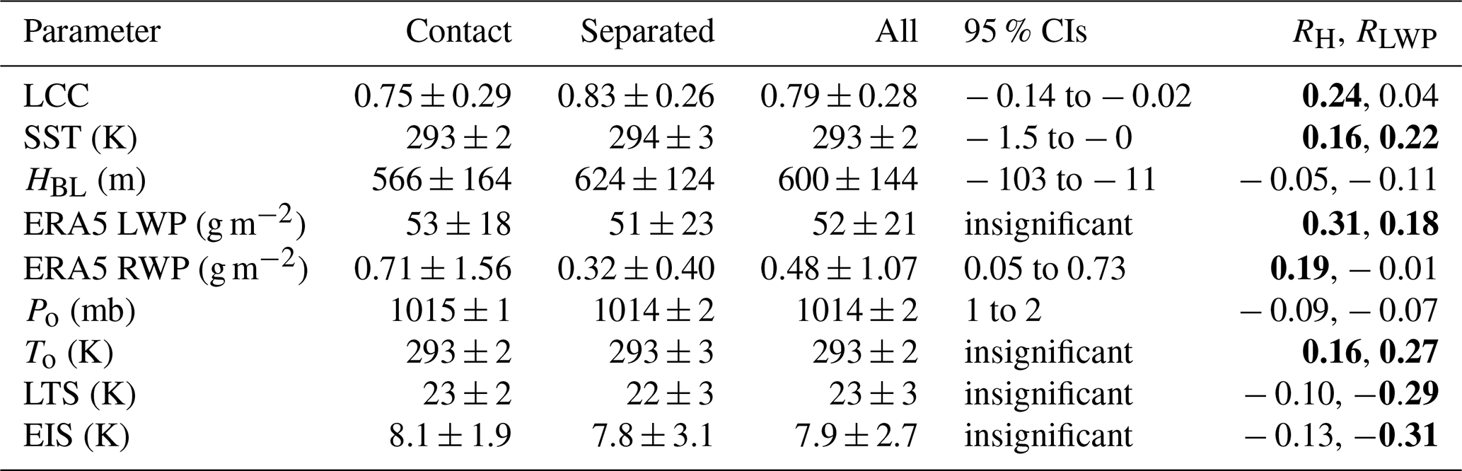
ERA5 provides hourly output with a horizontal resolution of $\mathrm{0.25}{}^{\circ }\times \mathrm{0.25}{}^{\circ }$ for 37 pressure (p) levels (up to 1 hPa). The cloud sampling for most flights was conducted within 3 h of 12:00 UTC (Table 2). ERA5 data at 12:00 UTC were thus used for the grid box nearest to the profile (Dzambo et al., 2019). The low cloud cover (LCC), SST, H_BL, total column liquid water (ERA5 LWP) and rainwater (ERA5 RWP), mean sea level pressure (p_o), 2 m temperature (T_o), and 2 m dew point temperature (T_d) were examined (Table 8).

Table 8 Meteorological and cloud properties from ERA5 reanalysis for contact, separated, and all profiles with LCC >0.95 (LCC is reported for all profiles), 95 % CIs from a two-sample t test applied to contact and separated profile data, and R between each parameter and LWP (R_LWP) or H (R_H) with statistically significant R_H and R_LWP in bold.

The difference between potential temperatures at 700 hPa and the surface was defined as LTS (Klein and Hartmann, 1993). EIS was calculated following Wood and Bretherton (2006):

$$\begin{array}{}\text{(9)}& \mathrm{EIS}=\mathrm{LTS}-{\mathrm{\Gamma }}_{\mathrm{m}}^{\mathrm{850}}\left(z_{\mathrm{700}}-\mathrm{LCL}\right),\mathrm{LCL}=\mathrm{125}\left(T_{\mathrm{o}}-T_{\mathrm{d}}\right),\end{array}$$

where Γ_m is the moist adiabatic potential temperature gradient, z₇₀₀ is the height at 700 mb, and LCL is the lifting condensation level (Lawrence, 2005). ${\mathrm{\Gamma }}_{\mathrm{m}}^{\mathrm{850}}$ is Γ_m for 850 hPa and calculated following Wood and Bretherton (2006).

LCC refers to cloud fraction for p>0.8p_o, corresponding to p>810 hPa, where most profiles were sampled (Table 2). The ECMWF model used a threshold of EIS >7 K to distinguish between well-mixed boundary layers topped by stratocumulus and decoupled boundary layers with cumulus clouds (ECMWF, 2020). This distinction improved the agreement between the model LCC and LWP and observations (Köhler et al., 2011). LCC was proportional to EIS $/$ LTS, and LCC <0.8 was mostly observed for EIS <7 K (Fig. 10a). Decoupled boundary layers can be topped by MSC (G21; Wood, 2012). Profiles with EIS <7 K were included in the analysis if ERA5 had LCC >0.95. This included 64 contact and 88 separated profiles from the three IOPs. For the 2016, 2017, and 2018 IOPs, 50, 20, and 76 profiles, respectively, had LCC >0.95 out of which 0, 4, and 44 profiles, respectively, had EIS <7 K. The average ERA5 H_BL (599±144 m) was lower than the average Z_T (932±196 m). This underestimation of H_BL by ERA5 has been observed for stratocumulus over the southeast and northeast Pacific (Ahlgrimm et al., 2009; Hannay et al., 2009).

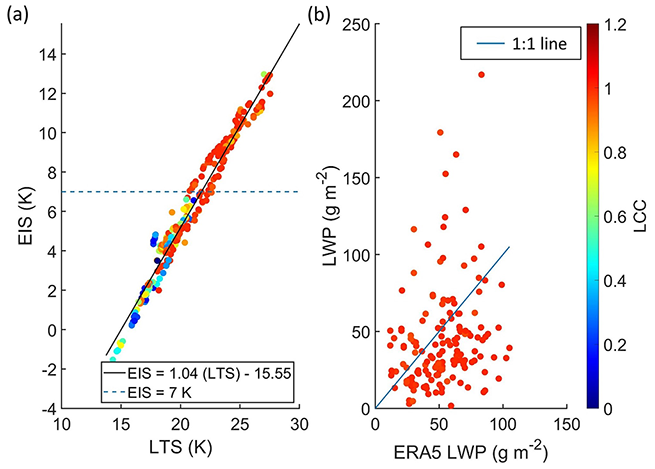
Figure 10 (a) LTS versus EIS with regression coefficients in legend (R= 0.98) and (b) LWP from size-resolved probes versus LWP from the ERA5 reanalysis (R=0.18) where each dot represents a single cloud profile. LTS, EIS, ERA5 LWP, and LCC for each cloud profile taken from the nearest ERA5 grid box (within 0.25^∘ of latitude and longitude) at 12:00 UTC. Panel (a) shows all cloud profiles and panel (b) shows cloud profiles with LCC >0.95.

On average, the ERA5 LWP (51±21 g m⁻²) was slightly greater than LWP (46±41 g m⁻²), but the differences were statistically insignificant. There was a significant but weak correlation between LWP and ERA5 LWP (R=0.18) (Fig. 10b). On average, the ERA5 RWP (0.48±1.07 g m⁻²) was lower than RWP (1.19±2.76 g m⁻²). There were insignificant differences between ERA5 LWP and LWP for contact and separated profiles with LCC >0.95 (Table 8). Contact profiles with LCC >0.95 had significantly higher ERA5 RWP (Table 8). While this is counterintuitive, given the precipitation suppression, it was due to the selection of profiles with LCC >0.95. Contact profiles with LCC >0.95 also had higher in situ RWP (95 % CIs: 0.32 to 2.08 g m⁻² higher) compared to separated profiles with LCC >0.95.

LWP was positively correlated with SST and T_o and negatively correlated with LTS and EIS with weak but statistically significant correlations (Fig. 11). On average, separated profiles had significantly higher SST (95 % CIs: 0.01 to 1.48 K higher) compared to contact profiles with insignificant differences between the average T_o, EIS, and LTS. Since the correlation between LWP $/$ H and SST was weak, it is unlikely the differences between contact and separated profiles were driven by SST differences alone. When all profiles (irrespective of LCC) were considered, there were insignificant differences between the average ERA5 RWP, SST, T_o, EIS, and LTS for contact and separated profiles. This suggests the differences between contact and separated profiles found during the ORACLES IOPs were primarily associated with ACIs instead of meteorological effects.

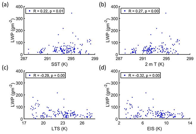
Figure 11 LWP from size-resolved probes as a function of (a) SST, (b) 2 m T, (c) LTS, and (d) EIS. Each dot represents a single cloud profile with LCC >0.95 and SST, 2 m T, LTS, and EIS taken from the nearest ERA5 grid box (within 0.25^∘ of latitude and longitude) at 12:00 UTC.

8 Conclusions

In situ measurements of stratocumulus over the Southeast Atlantic Ocean were collected during the NASA ORACLES field campaign. The microphysical (N_c and R_e), macrophysical (LWP and H), and precipitation properties (R_p and S_o) of the stratocumulus were analyzed. A total of 173 contact profiles with N_a>500 cm⁻³ within 100 m above cloud tops were compared with 156 separated profiles with N_a<500 cm⁻³ up to at least 100 m above cloud tops. Contact between above-cloud aerosols and the stratocumulus was associated with the following:

1. More numerous and smaller droplets with weaker droplet growth with height.

   Contact profiles had significantly higher N_c (84 to 90 cm⁻³ higher) and lower R_e (1.4 to 1.6 µm lower) compared to separated profiles. The median R_e had a smaller increase from cloud base to cloud top for contact (6.1 to 7.9 µm) compared to separated profiles (7.1 to 9.5 µm). The profiles had similar LWP and H, and it is hypothesized the differences in droplet growth were associated with collision–coalescence.

2. Aerosol-induced cloud microphysical changes in both clean and polluted boundary layers.

   Contact profiles had 25 to 31 cm⁻³ higher N_c and 0.2 to 0.5 µm lower R_e in clean and 98 to 108 cm⁻³ higher N_c and 1.6 to 1.8 µm lower R_e in polluted boundary layers compared to separated profiles. Contact profiles were more often located in polluted boundary layers and had higher below-cloud CO concentration (27 to 29 ppb higher), which suggests more frequent entrainment of biomass burning aerosols into the boundary layer compared to separated profiles.

3. Precipitation suppression with significantly lower precipitation intensity and precipitation formation process rates.

   Separated profiles had R_p up to 0.22 mm h⁻¹, while contact profiles had R_p up to 0.07 mm h⁻¹. S_AUTO and S_ACC had higher maxima for separated (up to $\mathrm{9.6}\times {\mathrm{10}}^{-\mathrm{10}}$ and $\mathrm{2.2}\times {\mathrm{10}}^{-\mathrm{8}}$ s⁻¹) compared to contact profiles (up to $\mathrm{2.9}\times {\mathrm{10}}^{-\mathrm{10}}$ and $\mathrm{1.2}\times {\mathrm{10}}^{-\mathrm{8}}$ s⁻¹).

4. Lower precipitation susceptibility, with the strongest impact in thin clouds (H<129 m).

   Contact profiles had lower S_o (0.87±0.04) compared to separated profiles (1.08±0.04). Thin clouds had the highest difference in S_o ($-\mathrm{0.06}\pm \mathrm{0.11}$ for contact and 1.47±0.10 for separated). Lower S_o for thin contact profiles was associated with poor correlation between N_c and R_p ($R=-\mathrm{0.03}$). For separated profiles, S_o decreased with H before increasing for H>256 m. In comparison, S_o increased with H for contact profiles for H>129 m.

5. Statistically insignificant differences in meteorological parameters that influence $\mathit{LWP}/H$.

   Based on ERA5 reanalysis data, LWP was correlated with SST (R=0.22), T_o (R=0.27), LTS ($R=-\mathrm{0.29}$), and EIS ($R=-\mathrm{0.31}$). Contact profiles with ERA5 LCC >0.95 had lower SST (0.01 to 1.48 K lower), with similar T_o, LTS, and EIS compared to separated profiles. The SST differences were insignificant when profiles with LCC <0.95 were included in the comparison.

Three important factors affecting S_o were discussed (Sorooshian et al., 2019): above-cloud N_a, below-cloud N_a, and meteorological conditions. This study analyzed ORACLES data from all three IOPs, and the first two conclusions were consistent with the analysis of ORACLES 2016 (Gupta et al., 2021). Future work will compare in situ data with R_p retrievals from APR-3 (Dzambo et al., 2021) to evaluate the sensitivity of S_o to the use of satellite retrievals of R_p (Bai et al., 2018). Vertical profiles of MSC properties will be used to evaluate satellite retrievals (Painemal and Zuidema, 2011; Zhang and Platnick, 2011) to address the uncertainties associated with satellite-based estimates of ACIs (Quaas et al., 2020). The ORACLES dataset can be combined with future investigations of marine stratocumulus to address the “lack of long-term datasets needed to provide statistical significance for a sufficiently large range of aerosol variability influencing specific cloud regimes over a range of macrophysical conditions” (Sorooshian et al., 2010).

Appendix A: Sensitivity studies on dependence of S_o on H

The base analysis examined how cloud properties varied with H by separating cloud profiles into four populations of H using the following endpoints: 28, 129, 175, 256, and 700 m. Two sensitivity studies determine if trends describing the variation of N_c, R_p, and S_o with H were sensitive to the endpoints used to sort cloud profiles into different populations.

First, cloud profiles were classified into two populations using the median H (175 m) to divide the populations (Table A1). The average N_c decreased, and the average R_p increased with H for both contact (211 to 186 cm⁻³ and 0.03 to 0.07 mm h⁻¹) and separated profiles (129 to 104 cm⁻³ and 0.07 to 0.15 mm h⁻¹). S_o increased with H for contact profiles from 0.53 to 1.06 and slightly decreased with H for separated profiles from 1.05 to 1.02 (Table A1). The difference between S_o for contact and separated profiles was greater for thin profiles (H<175 m) compared to thick profiles (H>175 m). These results are consistent with trends using four populations but provide less detail about how S_o varies with H (Fig. A1).

Figure A1 S_o as a function of H for contact and separated profiles classified into different populations using the endpoints indicated in legend. S_o was statistically insignificant when marked with a cross.

Table A1 S_o ± standard error with sample size and R in parentheses for contact, separated, and all profiles classified into a different number of populations.

Second, cloud profiles were classified into three populations using the terciles of H (145 and 224 m) (Table A1). The average N_c decreased, and the average R_p increased from the lowest to the highest H for contact (231 to 187 cm⁻³ and 0.03 to 0.07 mm h⁻¹) and separated profiles (138 to 95 cm⁻³ and 0.06 to 0.18 mm h⁻¹). For separated profiles, S_o first decreased with H from 1.15 to 0.25 before increasing to 1.45 for the highest H (Fig. A1). Contact profiles had insignificant S_o for the lowest H, followed by S_o increasing from 0.95 to 1.08 with H. The results presented here are robust with regards to the number of populations used.

Appendix B: Sensitivity studies on dependence of S_o on R_p

Another sensitivity study examined the R_p threshold used for cloud profiles included while calculating S_o. The average S_o decreased if weakly precipitating clouds with low R_p were excluded (Fig. B1, Table B1). It is possible that this was due to the higher N_a and N_c associated with weakly precipitating clouds. The exclusion of weakly precipitating clouds provides biased trends in S_o since these clouds could have undergone precipitation suppression already. Conversely, strongly precipitating clouds were associated with cleaner conditions and lower N_a and N_c. The exclusion of strongly precipitating clouds also leads to a decrease in the average S_o (Fig. B2, Table B1).

The occurrence of wet scavenging below strongly precipitating clouds (Duong et al., 2011) results in lower below-cloud N_a (and subsequently N_c). Higher susceptibility to precipitation suppression for cleaner, strongly precipitating clouds would explain the increase in the average S_o. This is consistent with observations of S_o using different R_p thresholds (see Fig B1, Jung et al., 2016) and hypotheses regarding the impact of different N_a on S_o (Duong et al., 2011; Fig. 11, Jung et al., 2016).

Table B1 S_o ± standard error with sample size and R in parentheses for contact, separated, and all profiles with R_p above a certain threshold.

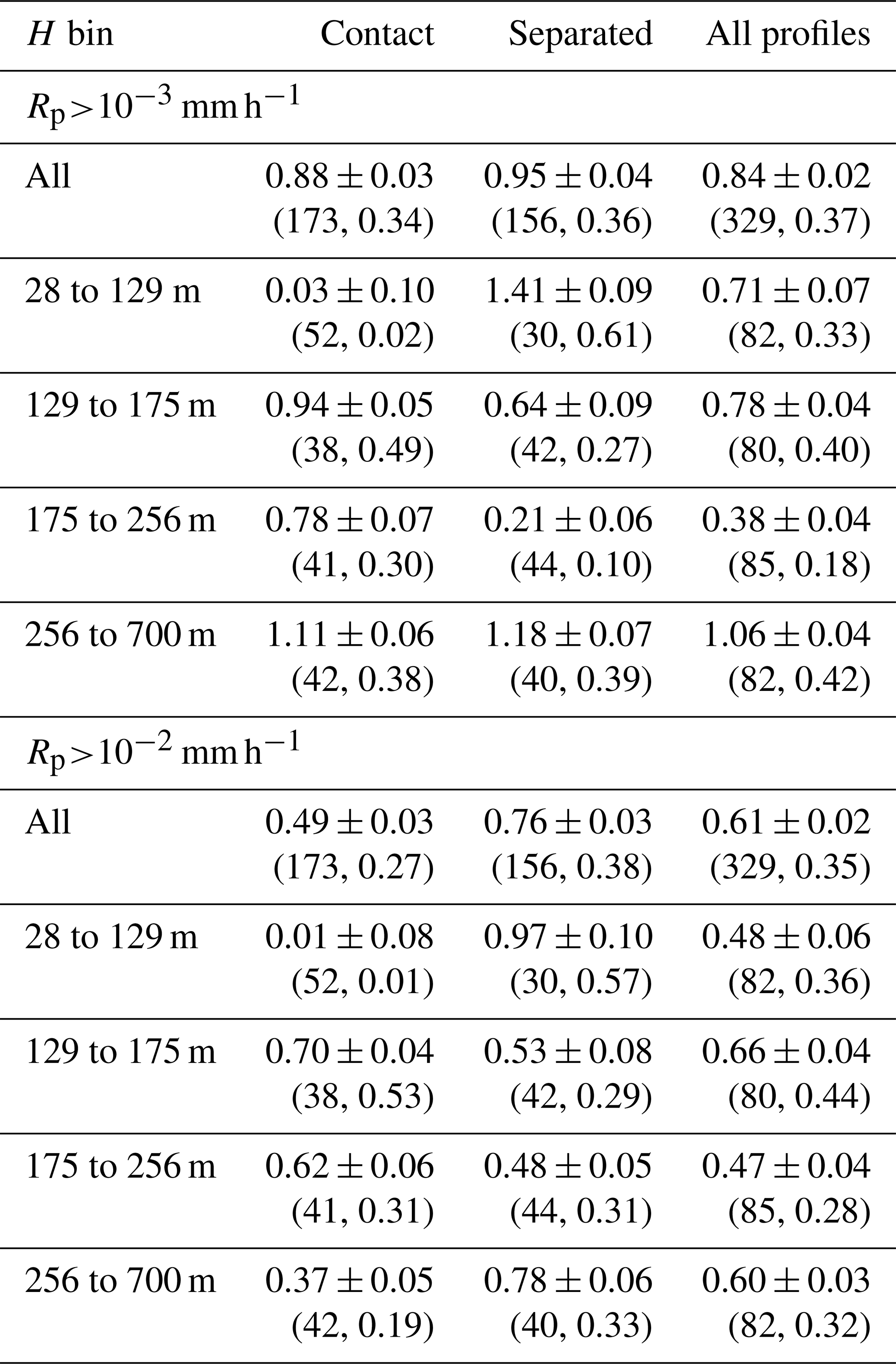
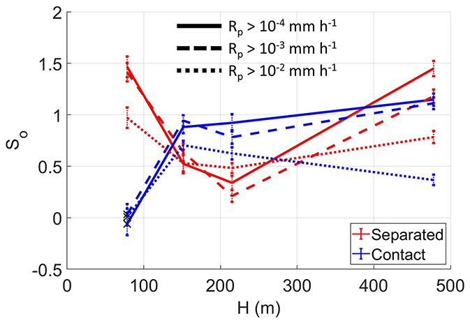
Figure B1 S_o as a function of H for contact and separated profiles, with R_p greater than the thresholds indicated in legend. S_o was statistically insignificant when marked with a cross.

Figure B2 S_o as a function of H for contact and separated profiles, with R_p less than the thresholds indicated in legend. S_o was statistically insignificant when marked with a cross.

Appendix C: Dependence of S_o on the definition of clean and polluted boundary layers

The number of cloud profiles classified into the S-L, C-L, S-H, and C-H regimes varied depending on the below-cloud N_a threshold used to define a low N_a or clean boundary layer. For the threshold used in the base analysis (350 cm⁻³), contact profiles were more often located in polluted boundary layers (131 out of 171 profiles classified as C-H) while separated profiles were more often located in clean boundary layers (108 out of 148 profiles classified as S-L). The comparisons between S_o in clean and polluted boundary layers varied with the threshold used.

As a sensitivity study, a lower threshold was used to define a clean boundary layer (300 cm⁻³). For this case, the C-L regime had no profiles in the population with the lowest H (H<129 m) when four populations of profiles were used to examine the dependence of S_o on H. Two out of the other three populations had an insignificant value for S_o due to poor and statistically insignificant correlations between N_c and R_p (Table C1). This was associated with a low sample size for the populations (six each). A second sensitivity study used a higher threshold to define a clean boundary layer (400 cm⁻³). For this case, the S-H regime has insignificant S_o for three out of the four populations of H and the remaining population had a small sample size (three profiles) (Table C1). The base analysis using a threshold of 350 cm⁻³ to define a clean boundary layer was used to compare S_o values that represent a larger number of cloud profiles.

Table C1 S_o ± standard error with sample size and R in parentheses for regimes defined in text and different thresholds to define a low N_a boundary layer. The use of italics denotes the statistical insignificance of S_o.

Appendix D: Sensitivity of S_o to the use of CAS data from ORACLES 2016

Given the differences between the CAS and PDI N_c and LWC for droplets with D<50 µm during ORACLES 2016 (see Supplement), sensitivity tests were performed by first excluding ORACLES 2016 data and second by using PDI data to represent ORACLES 2016 size distributions for D<50 µm in the S_o calculations. These sensitivity tests resulted in minor changes in the trends of S_o versus H (Fig. D1), along with average changes in the magnitude of S_o up to 0.05 (Table D1). The noted changes suggest that the discussion of trends in S_o described in this study is robust as it relates to the inclusion of ORACLES 2016 data and the use of CAS data for the deployment. Since the 2016 deployment contributed about a third of the ORACLES measurements, data from the 2016 deployment were included in the study so as not to reduce the size of the dataset.

The slight decrease in S_o for thick clouds (H>256 m) upon removal of ORACLES 2016 data is associated with a decrease in the number of thick clouds (Table D1). The use of PDI data resulted in minor changes because S_o primarily depends on N_c and R_p. The CAS and PDI datasets had small differences in the average N_c (95 % confidence intervals of 9 to 12 cm⁻³), and R_p was calculated using droplets with D>50 µm, which do not include contributions from either the CAS or the PDI. The documentation of differences between the ORACLES cloud probes (see Supplement) highlights the measurement uncertainties associated with the cloud probe datasets.

Table D1 S_o ± standard error for all profiles, with sample size and R in parentheses.

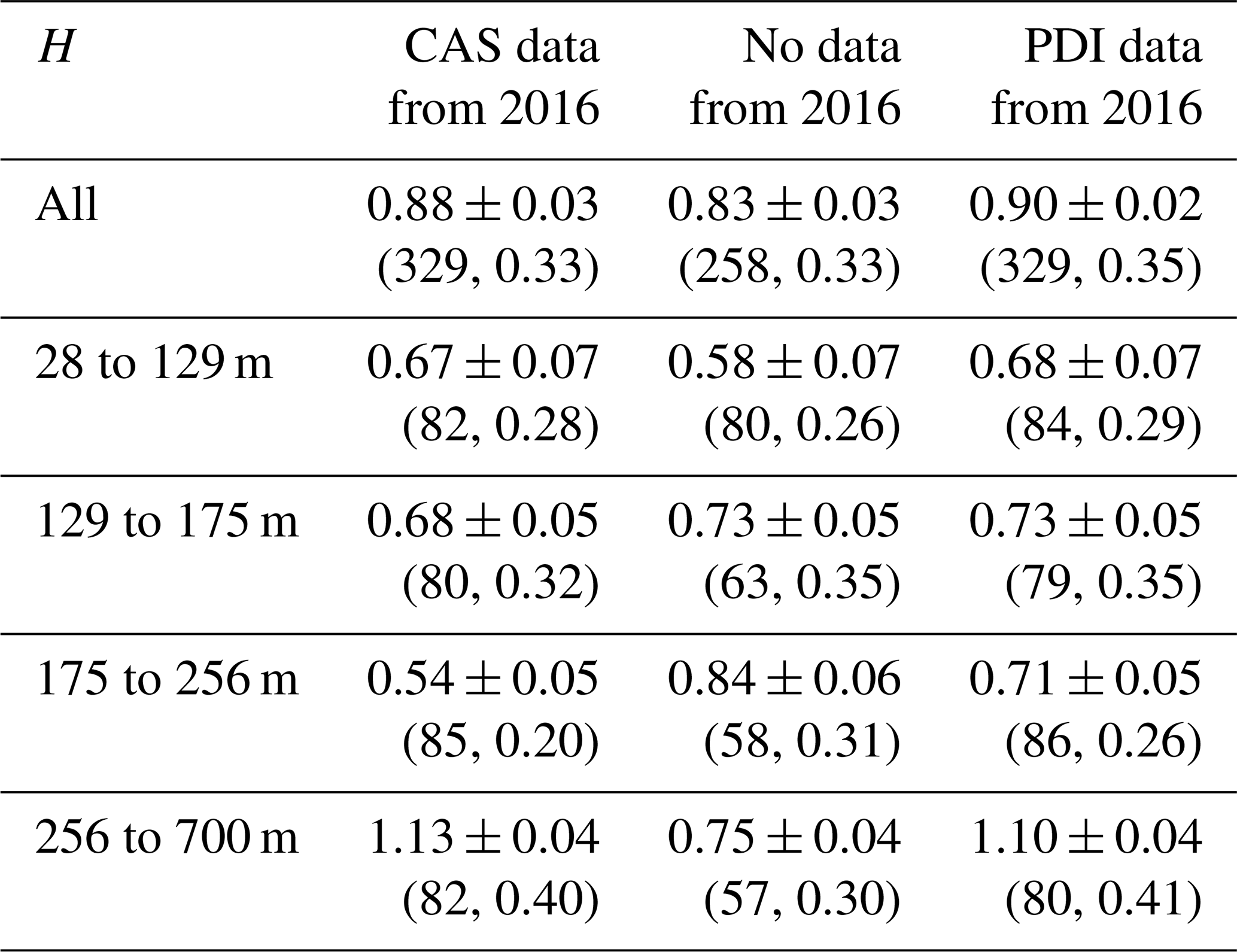
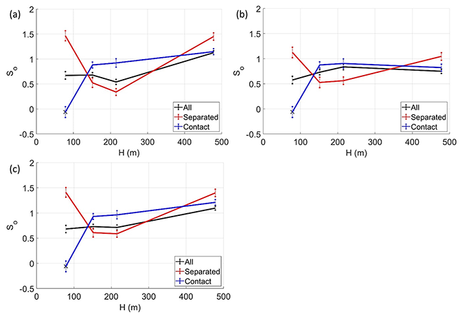
Figure D1 S_o as a function of H (error bars extend to standard error from regression model) using (a) CAS data, (b) no data, or (c) PDI data from ORACLES 2016.