Technical note: Dispersion of cooking-generated aerosols from an urban street canyon

The dispersion of cooking-generated aerosols from an urban street canyon is examined with building-resolving computational fluid dynamics (CFD). Using a comprehensive urban CFD model (PALM) with a sectional aerosol module (SALSA), emissions from deep-frying and boiling are considered for near-ground and elevated sources. With representative choices of the source flux, the inclusion of aerosol dynamic processes decreases the mean canyon-averaged number concentration by 15 %–40 % for cooking emissions, whereas the effect is significantly weaker for traffic-generated aerosols. The effects of deposition and coagulation are comparable for boiling, but coagulation dominates for deep-frying. Deposition is maximised inside the leeward corner vortices, while coagulation increases away from the source. The characteristic timescales are invoked to explain the spatial structure of deposition and coagulation. In particular, the relative difference between number concentrations for simulations with and without coagulation is strongly correlated with the ageing of particles along fluid trajectories or the mean tracer age. It is argued that, for a specific emission spectrum, the qualitative nature of the aerosol dynamics within urban canopies is determined by the ratio of the aerosol timescales to the relevant dynamical timescale (e.g. the mean age of air).

1 Introduction

Computational fluid dynamics (CFD) is a well-established tool for studying urban pollutant dispersion (e.g. Rivas et al., 2019). By including an explicit representation of buildings, urban flows can be simulated more accurately than is possible with coarse-resolution mesoscale atmospheric models (Park et al., 2015) or semi-analytical solutions like the classical Gaussian plume model (Melli and Runca, 1979). Most urban CFD studies assume neutral (uniform density) flow and passive scalar dynamics. In recent years, however, the accuracy of urban CFD models has been increased through the inclusion of additional physical processes such as solar heating (Nazarian and Kleissl, 2016) and gas-phase chemistry (Zhong et al., 2015).

One extension that has received relatively little attention is the inclusion of aerosol dynamic processes. The dynamics of urban aerosols differs from that of completely passive, neutrally buoyant particles because their evolution is affected by processes such as condensation, coagulation, deposition and nucleation (Seinfeld and Pandis, 2016); the importance of coagulation and deposition for urban nanoparticles has been noted by Karl et al. (2016). Since particulate matter poses potentially severe risks to human health (Greene and Morris, 2006), improved modelling of urban aerosols is desirable. Urban CFD studies of aerosols have examined ultra-fine particles (Nikolova et al., 2011; Scungio et al., 2013), PM_2.5 evolution (Zhang et al., 2011) and aerosol–chemistry coupling (Kim et al., 2012, 2019) arising from vehicular particle sources. Deposition is usually the only aerosol process included in urban CFD models as it is often taken to be the most important loss process of ultra-fine particles emitted by traffic (Kumar et al., 2011; Kim et al., 2019). Nevertheless, additional aerosol processes have been incorporated into global and regional atmospheric models using sectional aerosol modules in which the distribution of particles is represented with a set of discrete size bins (e.g. Gong et al., 2002). The sectional aerosol module SALSA (Kokkola et al., 2008) was coupled to the PALM urban CFD model by Kurppa et al. (2019) (hereafter K19), yielding good agreement with in situ measurements of the aerosol size spectrum.

Although numerical modelling of urban aerosols has focused on emissions from motor vehicles, other sources, such as ships (Ackerman et al., 1995) and factories (Purba and Tekasakul, 2012) also exist. Cooking-generated aerosols from restaurants can have a surprisingly large effect: in situ measurements conducted in a densely urbanised neighbourhood of Hong Kong show that the contribution of cooking emissions to organic aerosols may exceed that of motor vehicles (Lee et al., 2015; Liu et al., 2018). Despite their importance, little is known about the dynamics of cooking-generated aerosols in the outdoor environment; current understanding relies on in situ measurements and idealised laboratory experiments (Gao et al., 2015). The dispersion of cooking- and traffic-generated aerosols differs in two key respects. First, the size distribution of cooking emissions is shifted towards smaller particles as the proportion of particles with a diameter of O(10 nm) or less is much larger (See and Balasubramanian, 2006; Yeung and To, 2008). Hence the relative importance of the aerosol processes may change. Second, the particles are emitted from kitchen exhaust ducts, which may be located near the ground or far above it. Given that the dispersion of passive scalars is sensitive to the emission location (Huang et al., 2015; Duan et al., 2019), the aerosol dynamics and concentrations may be strongly affected.

In this paper, the dispersion of cooking-generated aerosols from a street canyon is analysed with large-eddy simulation (LES) and a sectional aerosol module. After reviewing the methodology (Sect. 2), results are presented for several idealised but generic emission scenarios, e.g. traffic, deep-frying and cooking emissions (Sect. 3). The aerosol dynamic processes are analysed in terms of the underlying aerosol timescales in Sect. 4 so as to highlight the key mechanisms. The sensitivity to factors such as the source strength and background aerosol concentrations is considered in Sect. 5. The robustness of the key findings, as well as the representativeness of the emission scenarios, is discussed in Sect. 6. Conclusions are given in Sect. 7.

2 Methodology

For simplicity, the dynamical core of the CFD model and the aerosol module are described separately.

2.1 Numerical formulation

2.1.1 PALM

The parallelised large-eddy simulation model (PALM) (Maronga et al., 2015) is an LES model based on the non-hydrostatic, filtered, incompressible Navier–Stokes equations. The 1.5-order Deardorff subgrid-scale (SGS) scheme (Deardorff, 1980) is used to parameterise SGS turbulent fluxes. Fifth-order differencing (Wicker and Skamarock, 2002) is combined with third-order Runge–Kutta time stepping (Williamson, 1980). While LES is more computationally expensive than the Reynolds-averaged Navier–Stokes (RANS) equations, the inclusion of transient dynamics allows for nonlinear aerosol processes (see Sect. 5.2) to be represented more accurately. With a steady model like RANS, temporal fluctuations are neglected, thereby necessitating a turbulence parameterisation for the aerosol dynamics.

2.1.2 SALSA

SALSA includes representations of condensation, coagulation, nucleation and dry deposition (Kokkola et al., 2008). Following K19, only dry deposition, coagulation and condensation are retained. Nucleation, which is most relevant in the immediate vicinity of the source (Rönkkö et al., 2007), can be treated by modifying the emissions (Ketzel and Berkowicz, 2004) and is not considered in this work. Details on the implementation are given in Appendix A. Briefly, deposition removes particles near surfaces: the deposition velocity is non-zero within the first grid box at a surface, e.g. from z=0 to z=Δz (see Fig. 13a); away from the surface, only gravitational settling occurs. Coagulation coalesces smaller particles into larger ones, decreasing the number concentration but shifting the size distribution; condensation of gases onto particles gases changes the aerosol concentration. As with other sectional models, the parameterisations depend on the particle size. SALSA divides the size distribution into several subranges, each of which is discretised into a specified number of size bins based on the particle diameter, D_p. We adopt the same partitioning as K19: in subrange 1, $D_{\text{p}}\in [\mathrm{3},\mathrm{50}\mathrm{nm}]$; in subrange 2, D_p>50 nm. The particle number in each size bin, n_i, is a prognostic variable. The total particle number $N={\sum }_i{n}_i$.

Particles are introduced via injection of a specific component or through condensation of gaseous components. The chemical components include organic carbon (OC), black carbon (BC), sulfuric acid (H₂SO₄), nitric acid (HNO₃), ammonium (NH₃), sea salt, dust and water (H₂O). Subrange 1 includes OC, H₂SO₄, HNO₃ and NH₃ only, which are assumed to be internally mixed; subrange 2 includes all the chemical components. Gaseous components, namely H₂SO₄, HNO₃, NH₃, semi-volatile organics (SVOCs) and non-volatile organics (NVOCs), may condense onto particles; however, gas-phase chemical reactions are excluded.

2.2 Configuration

2.2.1 PALM

An idealised single street canyon of unit aspect ratio, i.e. with dimensional building height H=20 m and width W=20 m, is located at the centre of the computational domain (Fig. 1a). The domain has dimensions 5H, 2H and 5H in the streamwise (x), spanwise (y) and vertical (z) directions, respectively; the spanwise extent is somewhat limited but comparable to that of previous studies (e.g. Baik et al., 2007; Duan et al., 2019). The uniform, isotropic grid spacing Δ=1 m. The time step Δt_PALM is ∼0.1 s.

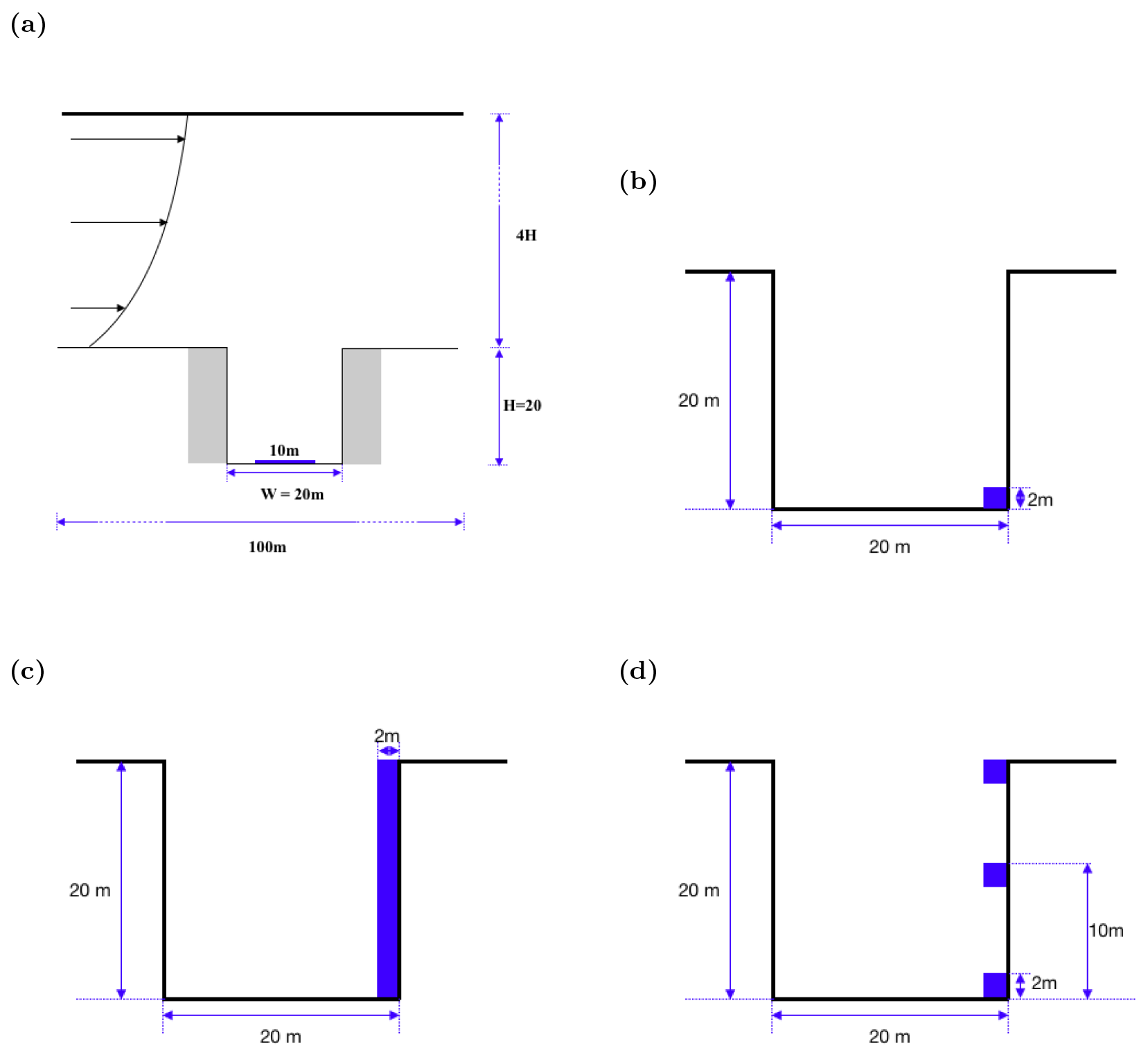
Figure 1 Schematic representations in the x–z plane (at the midplane $y/W$ = 1) of the computational domain and pollutant sources: (a) ground-level traffic emissions; (b) near-ground cooking emissions; (c) column cooking emissions; (d) isolated cooking emissions. The emission scenarios are defined in Table 1. For clarity, the streamwise position of the cooking sources has been shifted.

The boundary conditions follow previous studies. For the velocity, cyclic boundary conditions are applied in the streamwise and spanwise directions, free slip at the top and no slip at all solid surfaces. For scalar quantities (including the particle number in each size bin), there are cyclic boundary conditions in the spanwise direction and Dirichlet (e.g. n_i=0) in the streamwise direction. The flow is driven by an external pressure gradient, $\mathrm{d}p/\mathrm{d}x=-\mathrm{0.0006}\mathrm{Pa}{\mathrm{m}}^{-\mathrm{1}}$. This value has been widely used in previous CFD studies (e.g. Duan et al., 2019); it yields a streamwise velocity $U\sim \mathrm{3}{\mathrm{ms}}^{-\mathrm{1}}$ at $z/H=\mathrm{2.5}$. The simulations are conducted under neutral conditions with the temperature fixed at 300 K.

The configuration described above differs in several respects from K19. First, an idealised street canyon is used in place of realistic topography within a neighbourhood-scale domain. Second, there is uniform grid spacing rather than a stretched grid. Third, the computational lid height of 5H is decreased from 13H_avg, where H_avg is the mean building height.

The model was spun up for 1000 s in order to attain a statistically steady flow (as determined from the mean streamwise velocity within the canyon). Subsequently particle emission commenced and the model was run for another 5000 s. Data collected during the last 3000 s (with an output interval of 10 s) are analysed in this study. During the 3000 s sampling period, the number concentration also reaches statistical distribution: the ratio of the standard deviation to the mean is around 6 %

The time average is denoted by the overbar. The spanwise average is denoted by 〈⋅〉 and the canyon average by 〈〉_c.

Figure 2 shows mean streamlines and wind speed in the x–z plane. The picture is consistent with the many numerical studies of unit-aspect-ratio street-canyon flow. In particular, there is a large central vortex and smaller canyon vortices. Although the corner vortices are not defined as clearly as in higher-resolution simulations e.g. Duan et al. (2019), recirculations clearly exist within the bottom corners. Ramifications of the streamline topology are considered in Sect. 3.

2.2.2 SALSA

Version 4481 of SALSA is used. Following K19, there are five size bins for each of the two subranges. As the current study is concerned with idealised emission scenarios, the background number concentration for the ith size bin, $n_{\mathrm{b},i}=\mathrm{0}$; the sensitivity to n_b,i is examined in Sect. 5.1. As in K19, the SALSA time step Δt_SALSA=1 s in all cases. The three aerosol processes in SALSA (coagulation, condensation and deposition) may be activated or deactivated independently of each other.

Pollutants are emitted from uniform area sources. Since aerosol emissions are handled by SALSA rather than PALM, pollutants are subjected to aerosol dynamic processes before being transported and advected by PALM. Two basic source types are considered: (i) ground-level traffic and (ii) cooking emissions from one side of a street canyon. In the former case, a uniform area source is located at the bottom of the canyon. In the latter case, the sources, which cover a portion of the walls facing the street, are located at the roadside (Fig. 1b); between the ground and the roof level (Fig. 1c); and at the bottom, middle or top floors (Fig. 1d). No attempt is made to represent exhaust ducts. These sources represent roadside and elevated (aligned in a column or else isolated) kitchens. In addition, there are two possible cooking modes, namely deep-frying and boiling: both are considered as their emission spectra are rather different (Fig. 3).

2.2.3 Emission scenarios

For each source type, the emission spectra and source flux (${\mathrm{m}}^{-\mathrm{2}}{\mathrm{s}}^{-\mathrm{1}}$) must be specified. Values that are broadly representative of large cities are chosen for the latter. The sensitivity to the net source flux is quantified in Sect. 5.2.

1. Ground-level traffic (Case TR). The emission factor for the number of particles emitted by a vehicle per unit distance travelled was estimated to be 3.0×10¹⁴ km⁻¹ per vehicle (Fujitani et al., 2020). A traffic volume of 1000 vehicles per hour, which corresponds to moderately heavy traffic within a city centre, is assumed. The total particle flux (s⁻¹), T_p, is obtained from the emission factor and the length of the street, i.e. T_p=ϵL, from which the source flux $Q=T_{\text{p}}/A$, where A is the area covered by the traffic.

2. Cooking emissions. The emission factors for the number of particles emitted per unit time by a kitchen of unit volume were estimated to be $\mathrm{3.75}\times {\mathrm{10}}^{\mathrm{10}}{\mathrm{m}}^{-\mathrm{3}}{\mathrm{s}}^{-\mathrm{1}}$ and $\mathrm{4.31}\times {\mathrm{10}}^{\mathrm{9}}{\mathrm{m}}^{-\mathrm{3}}{\mathrm{s}}^{-\mathrm{1}}$, for deep-frying and boiling, respectively. These values are derived from data for reference kitchens with a volume of ∼20 m³; it is assumed that no particles are trapped indoors.

   The total particle flux (s⁻¹) is obtained from the emission factor and the volume of the kitchens, i.e. T_p=nϵV, where V is the volume and n is the number of kitchens. It is assumed for simplicity that particles are emitted uniformly over the external face of the restaurant. The source flux follows from normalisation by A, the area of the kitchen face parallel to the canyon axis. The indoor–outdoor exchange is entirely one-way: particles escape from the kitchens to the outdoor environment, but no particles travel in the opposite direction.

   The source specification depends on the emission scenario (Table 1).

   • Near-ground emissions (Case NG). It is assumed that each roadside kitchen has dimensions $\mathrm{4}\text{m}\times \mathrm{2}\text{m}\times \mathrm{2}\text{m}$, with the longest side being parallel to the street. Hence the total particle flux equals the combined emissions from 10 restaurants.

   • Column emissions (Case CO). There are a total of five elevated kitchens between the bottom and top floors. The kitchens may be taken to be domestic rather than commercial and of smaller dimensions, namely $\mathrm{2}\text{m}\times \mathrm{2}\text{m}\times \mathrm{4}\text{m}$. For simplicity, the combined emissions from the separate kitchens are represented by a continuous column source.

   • Isolated emissions (Case I). Only a single elevated kitchen is considered. It has dimensions $\mathrm{2}\text{m}\times \mathrm{2}\text{m}\times \mathrm{4}\text{m}$.

   Emission spectra are obtained by scaling the reference spectra (Fig. 3); the contribution of a specific size bin is determined by T_p and the emission spectrum. No attempt is made to represent the kitchen ventilation system; hence all indoor aerosol processes are excluded. The scaling factor for a size bin is given by the ratio of the integral of the emission spectrum over the size bin to the integral over the entire spectrum. Note that, for a kitchen of identical size, deep-frying generates nearly 10 times as many particles as does boiling. In addition, more small particles are generated for deep-frying: the proportion of nanoparticles in the 1 to 100 nm range increases from 65 % to 90 %, and the mean diameter decreases from 57.4 to 26.5 nm (See and Balasubramanian, 2006; Yeung and To, 2008). However, the boiling spectrum peaks at a smaller diameter.

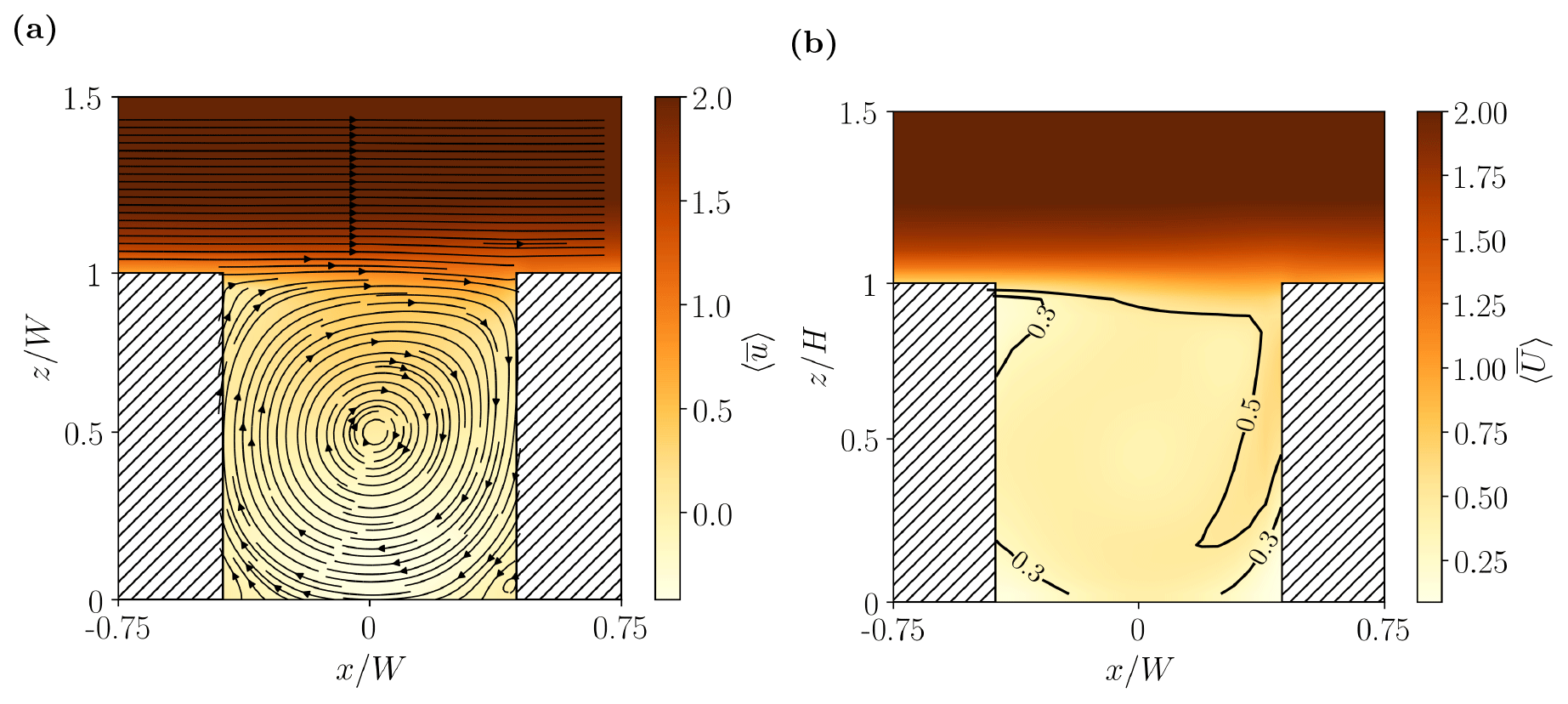
Figure 2 Spatial structure of the mean flow in the x–z plane: (a) streamwise velocity component, u (m s⁻¹); (b) wind speed, U (m s⁻¹).

The emission scenarios described above are summarised in Table 1.

Several assumptions are required to specify the particle emissions from cooking; their validity is discussed in Sect. 6. The gaseous emissions are specified in Appendix B: in particular, the chemical compositions (Table B1) and emission factors (Table B2) are listed.

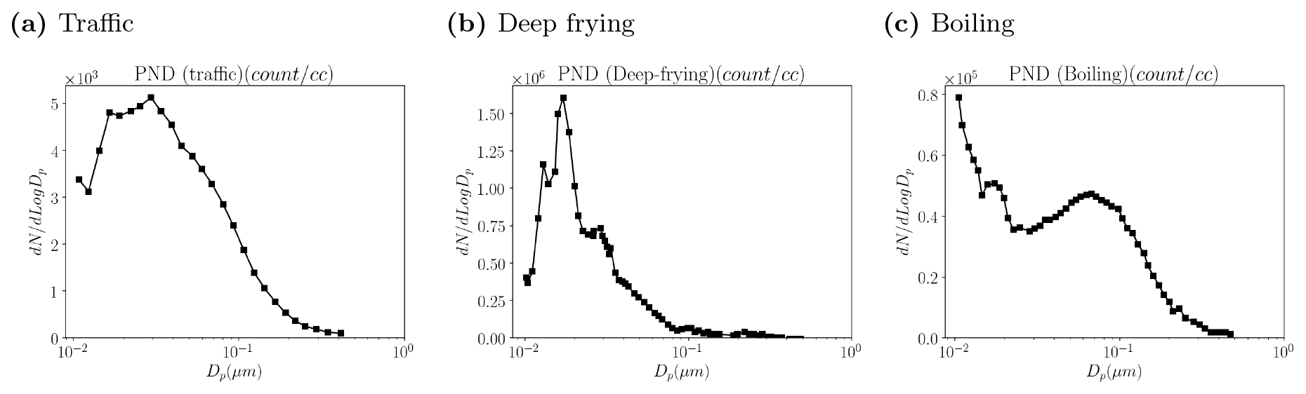
Figure 3 Reference emission spectra: (a) traffic (Janhäll et al., 2004); (b) deep-frying (See and Balasubramanian, 2006); (c) boiling (See and Balasubramanian, 2006). The reference spectra are scaled in order to obtain emission spectra for the scenarios of Table 1.

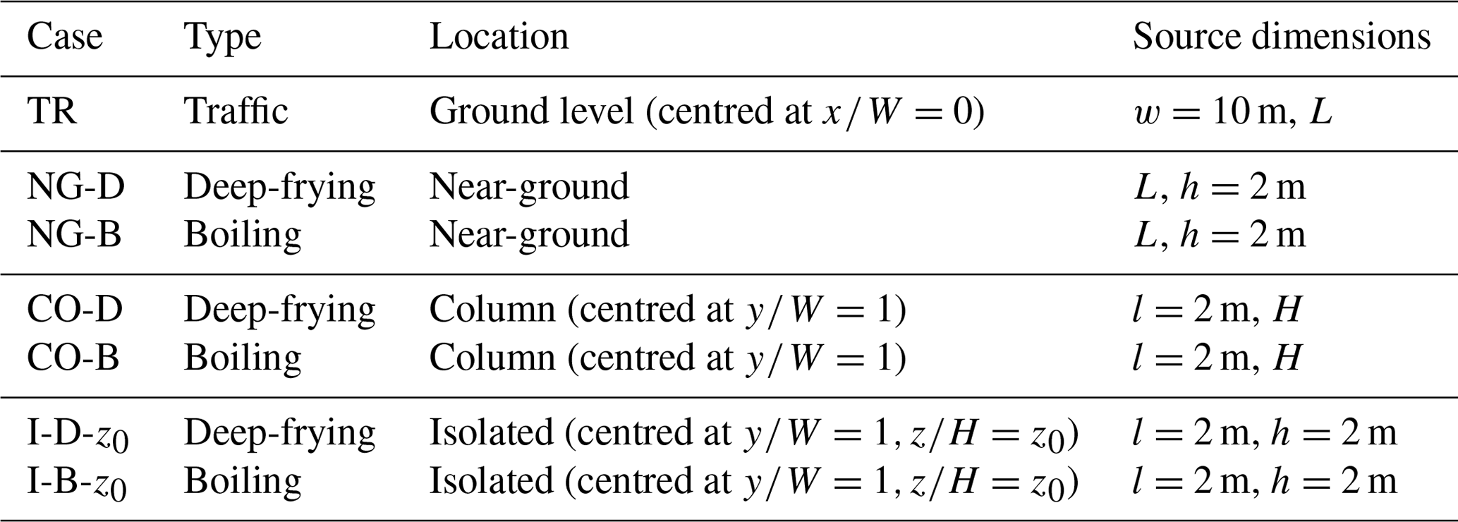
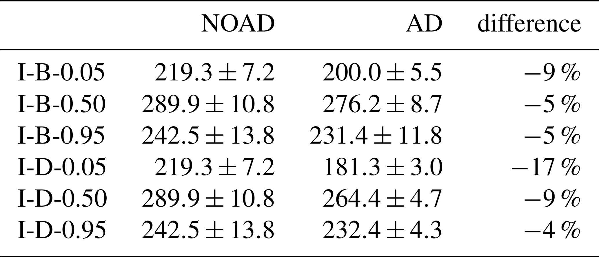
Table 1 Emission scenarios for the area sources illustrated in Fig. 1. The dimensions of the area sources are expressed in terms of the canyon dimensions $(W,L,H)$ when the source extends along the full extent of the canyon in a given direction, and $(w,l,h)$ otherwise. For the isolated cooking emissions, $z_{\mathrm{0}}/H\in \mathit{\{}\mathrm{0.05},\mathrm{0.50},\mathrm{0.95}\mathit{\}}$.

2.3 Validation

Several validation tests have been performed. First, the mean velocity statistics are validated against measurements of flow over parallel unit-aspect-ratio streets canyons (Brown et al., 2001). Second, passive scalar statistics are also validated (Pavageau and Schatzmann, 1999). Finally, the performance of the coupled PALM–SALSA model is compared to previous studies (Kumar et al., 2008; Kurppa et al., 2019).

With respect to the uncoupled CFD model, as shown in Fig. 4, vertical profiles of the mean streamwise velocity u show good agreement with the measurements at different streamwise locations and $z/H\le \mathrm{1.5}$ when the PALM configuration of Sect. 2.2.1 is used. Standard validation metrics (Appendix C) confirm that the validation is successful: with the normalised mean square error $\text{NMSE}\sim \mathrm{0.01}-\mathrm{0.04}$, fractional bias FB ∼ 0.02 and correlation coefficient R∼0.99. For a perfect validation, $\text{NMSE}=\text{FB}=\mathrm{0}$ and R=1. The agreement is comparable to previous numerical studies (Cui et al., 2004; Duan et al., 2019). Passive scalar statistics for a ground-level line source (see Sect. 2.2 for configuration details) also show good agreement. For example, NMSE=0.07 and FB = 0.02 (cf. Fig. C1). We conclude that PALM is capable of simulating the mean flow and an accompanying passive scalar.

With respect to the coupled PALM–SALSA model, vertical profiles of aerosol number concentration are validated against evening measurements made within a real street canyon in Cambridge, UK (Kumar et al., 2008). For simplicity, the computational domain is focused on this street canyon: no other buildings are included. In particular, a single street canyon of $\mathrm{167}\text{m}\times \mathrm{12}\text{m}\times \mathrm{12}\text{m}$ is centred inside a domain of $\mathrm{167}\text{m}\times \mathrm{60}\text{m}\times \mathrm{60}\text{m}.$ For consistency with the evening measurements, the temperature is fixed at 274 K. Using the background concentrations and traffic counts of Kumar et al. (2008), emissions from the street canyon only are considered. Aside from the computational domain and source specification, the distribution of size bins is adjusted to match PALM and SALSA configurations following Sect. 2.2. Vertical profiles of the aerosol number concentration are compared in Fig. 5. Compared to K19, the current LES shows improved agreement with in situ measurements for $z/H\mathit{\lesssim }\mathrm{0.6}$, though there are fairly large errors in both cases. The improved agreement may be fortuitous inasmuch as the present validation neglects emissions from outside the street canyon; nevertheless, the present configuration simulates the aerosol distribution in the real urban environment at least as well.

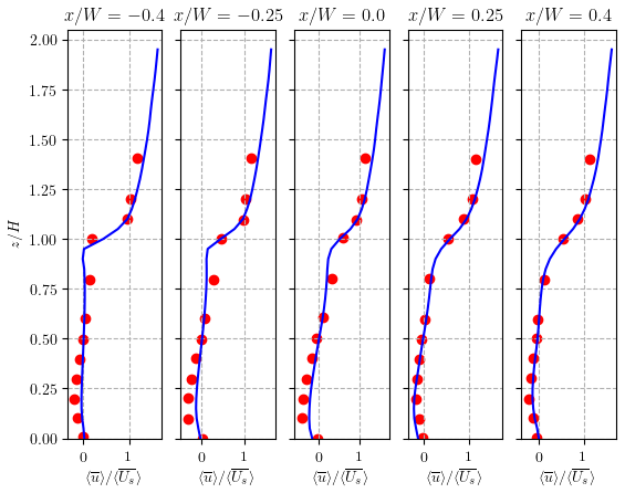
Figure 4 Vertical profiles of the normalised mean streamwise velocity, $\langle \stackrel{\mathrm{‾}}{u}\rangle /\langle \stackrel{\mathrm{‾}}{U_{\text{s}}}\rangle$, for the present LES and wind-tunnel measurements (Brown et al., 2001). $\langle \stackrel{\mathrm{‾}}{U_{\text{s}}}\rangle$ is the average streamwise velocity within the shear layer ($\mathrm{1}\le z/H\le \mathrm{1.5}$). The LES results are plotted with blue lines and the wind-tunnel data with red circles.

Figure 5 Vertical profiles of the aerosol number concentration within a street canyon in Cambridge, UK. The original in situ evening measurements (Kumar et al., 2008) are plotted in red. LES simulations using PALM–SALSA from K19 and the current study are plotted in black and blue, respectively. Error bars (standard deviations) for the current LES are plotted with horizontal lines.

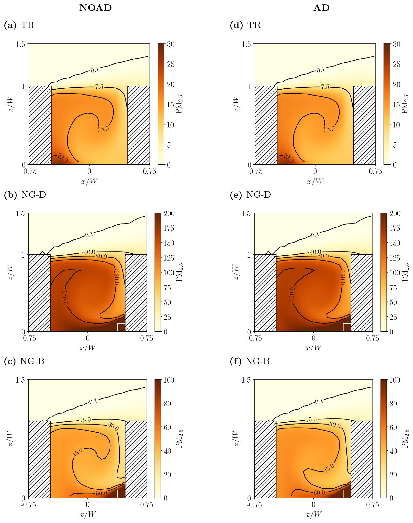
Figure 6 Normalised mean aerosol number concentration, $\langle \stackrel{\mathrm{‾}}{N_{*}}\rangle$, for different emission scenarios: (a, b) traffic (Case TR); (c, d) near-ground, deep-frying (Case NG-D); (e, f) near-ground, boiling (Case NG-B). Results without (NOAD) and with (AD) aerosol dynamic processes are shown at the left and right, respectively. The approximate position of the roadside restaurants is indicated by the white lines (which are shifted for clarity).

3 Results

3.1 Traffic and near-ground cooking emissions

To highlight the influence of the emission spectrum, we begin by comparing the aerosol number concentration fields generated by traffic and roadside restaurants, i.e. emission scenarios TR, NG-D and NG-B (Table 1). Figure 6 plots spanwise averages of the dimensionless mean concentrations,

$$\begin{array}{}\text{(1)}& \stackrel{\mathrm{‾}}{N_{*}}={\displaystyle \frac{\stackrel{\mathrm{‾}}{N}{U}_{\mathrm{ref}}HL}{T_{\text{p}}}},\end{array}$$

where $\stackrel{\mathrm{‾}}{N}$ is the time-averaged total number concentration (m⁻³) and U_ref (m s⁻¹) is the streamwise velocity at 2.5H. In the absence of aerosol dynamic processes (NOAD, left panels), the number concentration is essentially a passive scalar. For traffic emissions from the ground-level source (Fig. 6a), there are elevated concentrations within and around the vortex at the bottom leeward corner, as has been observed in many studies (for the related case of a line source see Pavageau and Schatzmann, 1999). For roadside cooking emissions from the windward side (Fig. 6b, c), pollutants recirculate around the corner before they can disperse through the rest of the canyon. Similar results for a pair of line sources were obtained by Huang et al. (2015); the fluid-dynamical processes governing escape from the corner vortex are discussed by Duan et al. (2019), who analysed the initial-value problem rather than the forced one. Deep-frying (NG-D) and boiling (NG-B) yield identical normalised concentrations in the absence of aerosol dynamic processes. In all cases, the concentration field reflects the combined influence of the mean flow (streamline geometry) and source location. Canyon-averaged number concentrations are summarised in Table 2.

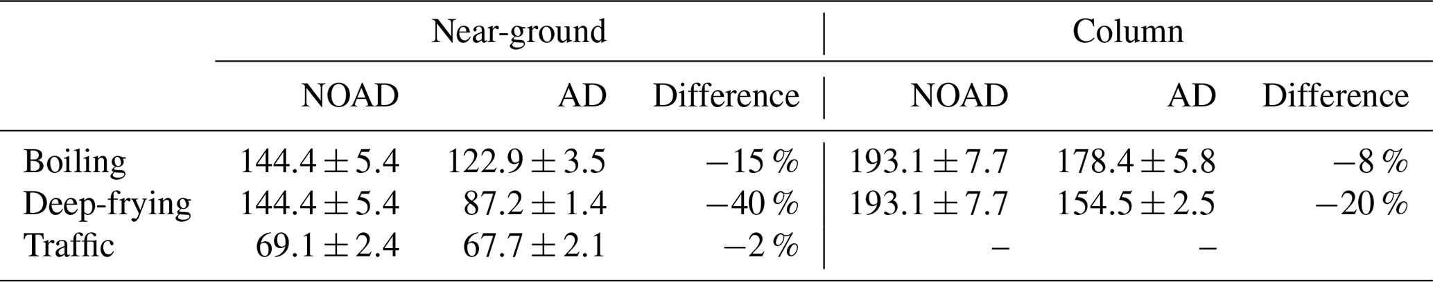
Table 2 Canyon-averaged dimensionless concentrations, $\langle \stackrel{\mathrm{‾}}{N}{\rangle }_{\text{c}}$, for the near-ground (Fig. 6) and column (Fig. 7) cooking emissions. The errors correspond to the spatial standard deviation; the relative change in the mean concentrations is also listed. Both the mean and standard deviation are time-averaged.

The effect of aerosol dynamic processes (AD) is illustrated by the right panels. For traffic emissions, the spatial structure of the number concentration field is almost identical (Fig. 6b), while the canyon-averaged and pedestrian-level concentrations decrease by around 2 %. In their study of a neighbourhood in Cambridge, UK, K19 found that aerosol processes cause the number concentration to decrease by ∼10 %. One possible explanation for this discrepancy is that the emission spectra differ: the mean particle size is larger in the current study, i.e. 47.9 nm rather than 32.7 nm. This is significant because smaller particles (with a diameter less than 100 nm; K19) may have a larger deposition velocity, leading to enhanced deposition (see Sect. 3.3.2 for further discussion). For cooking emissions, the spatial structure of the concentration fields and the mean values change. With deep-frying (Fig. 6d), the highest concentrations (shown in red) are confined to a smaller region in the windward corner and the isolines are strongly perturbed. With boiling (Fig. 6f), the highest concentrations are confined to a larger region and the isolines are deflected, though not as dramatically as for deep-frying. The canyon-averaged concentrations decrease by 15 % for boiling and 40 % for deep-frying. Since cooking, whether through boiling or deep-frying, generates more small particles than does traffic (Fig. 3), the coagulation and dry deposition rates should be higher.

Of course the results will differ with other assumptions about the kitchen dimensions (Sect. 2.2.2). The sensitivity to the source flux is examined in Sect. 5.2.

For reference, mass concentration fields are shown in Appendix D. In general, PM_2.5 mass concentrations (i.e. for particles smaller than 2.5 µm in diameter) are higher for cooking emissions, especially for deep-frying. Indeed the maximum concentration for NG-D reaches 200 µg m⁻³ near the source region (Fig. D1); possible reasons for these high values are given in Sect. 6. In agreement with the measurement campaign of Lee et al. (2015), the local contribution of cooking emissions exceeds that of traffic. However, the mass concentration shows much less sensitivity to the inclusion of aerosol processes.

Figure 7 As in Fig. 6 but for column cooking emissions: (a, b) deep-frying; (c, d) boiling.

3.2 Elevated kitchens

Kitchens may not be located at the roadside. This section considers continuous emissions along a column extending from the bottom to top of a building, as well as isolated kitchens on different levels.

The qualitative effect of column cooking emissions resembles the near-ground emissions. For both deep-frying and boiling, the familiar pattern of very high concentrations in the bottom leeward corner and lower concentrations aloft is maintained (Fig. 7); however, the concentrations increase in the interior. Averaged over the canyon, the spatial mean and standard deviation increase for column emissions (Table 2), but the sensitivity to aerosol processes weakens: the difference between NOAD and AD is 8 % and 20 % for boiling and deep-frying, respectively.

If the number concentration depended linearly on particle emissions, the nondimensionalisation would remove the dependence on the total particle flux, T_p; nonlinear effects are discussed in Sect. 5.1.

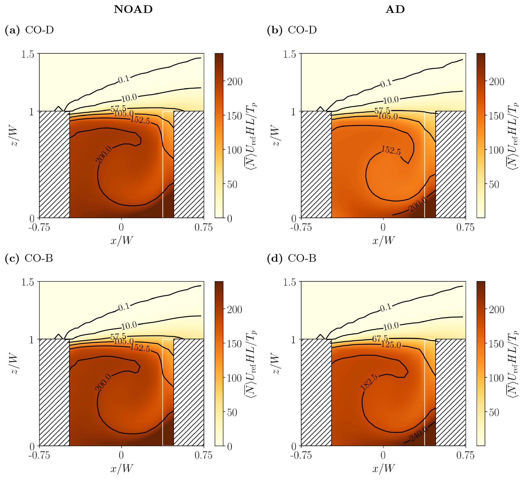
The influence of the source height is stronger for the isolated kitchens. Normalised mean aerosol number concentrations for I-B-z₀ are shown in Fig. 8. Although, trapping of particles within the vortex at the bottom leeward corner is less evident as the source height is increased from $z_{\mathrm{0}}/H=\mathrm{0.05}$ to $z_{\mathrm{0}}/H=\mathrm{0.95}$ (Fig. 8a–c), as the contrast with the interior weakens, but emission from the elevated sources actually increases the canyon-averaged concentrations. The vertical profiles (Fig. 8d) show that concentrations are maximised for $z_{\mathrm{0}}/H=\mathrm{0.5}$, which is consistent with elevated concentrations around the central canyon vortex (Duan et al., 2019). Canyon averages show that the effect of the aerosol processes is greatest for ground-level emission, $z_{\mathrm{0}}/H=\mathrm{0.05}$ (Table 3). The results for I-D-z₀ are similar (Fig. S1).

Figure 8 As in Fig. 6 but for isolated kitchens and boiling. The kitchens are located at (a) $z/H=\mathrm{0.05}$, (b) $z/H=\mathrm{0.5}$ and (c) $z/H=\mathrm{0.95}$. Mean vertical profiles are plotted in panel (d).

Table 3 As in Table 2 but for deep-frying and boiling emissions from isolated kitchens.

3.3 Comparison of aerosol dynamic processes

The effect of the individual aerosol processes is assessed by analysing separate SALSA configurations in which condensation, coagulation, and deposition, or all three processes acting simultaneously, are enabled. As in K19, the relative difference,

$$\begin{array}{}\text{(2)}& {\text{RD}}_i={\displaystyle \frac{\langle \stackrel{\mathrm{‾}}{N_{\text{NOAD}}}\rangle -\langle \stackrel{\mathrm{‾}}{N_i}\rangle }{\langle \stackrel{\mathrm{‾}}{N_{\text{NOAD}}}\rangle }},\end{array}$$

is defined from the mean concentrations with aerosol processes, $\langle \stackrel{\mathrm{‾}}{N_i}\rangle$, and without them, $\langle \stackrel{\mathrm{‾}}{N_{\text{NOAD}}}\rangle$. In the former case, $i\in \mathit{\{}\mathrm{COND},\mathrm{COAG},\mathrm{DEPO},\mathrm{ALL}\mathit{\}}$ labels the different SALSA configurations. The subscript is dropped when there is no risk of confusion. For brevity, not all of the emission scenarios listed in Table 1 are analysed here. Results for boiling may be found in Figs. S2 and S3).

3.3.1 Traffic emissions

Figure 9 compares the effects of the different aerosol processes for traffic emissions. Vertical profiles of the mean number concentration have nearly identical shapes for the different configurations (Fig. 9a). The lowest concentrations are obtained for deposition only. On account of nonlinearity, the effects do not add linearly.

By contrast with K19, who considered a domain with uneven building heights, the relative difference shows minimal variation with height (Fig. 9b). Condensation has a negligible effect on the aerosol number concentration, which is consistent with the notion that it primarily serves to increase the volume of particles (Seinfeld and Pandis, 2016). The effects of deposition and coagulation are approximately constant away from the bottom boundary. For $z/H>\mathrm{0.2}$, RD is ∼4.5 % for deposition and ∼0.4 % for coagulation. The estimate of RD_DEPO is low compared to K19, who obtained RD_DEPO∼15 % using a different emission spectrum, non-zero background concentration and realistic urban topography. Nonetheless, deposition remains the most important process for traffic emissions, in agreement with the timescale analysis of Ketzel and Berkowicz (2004).

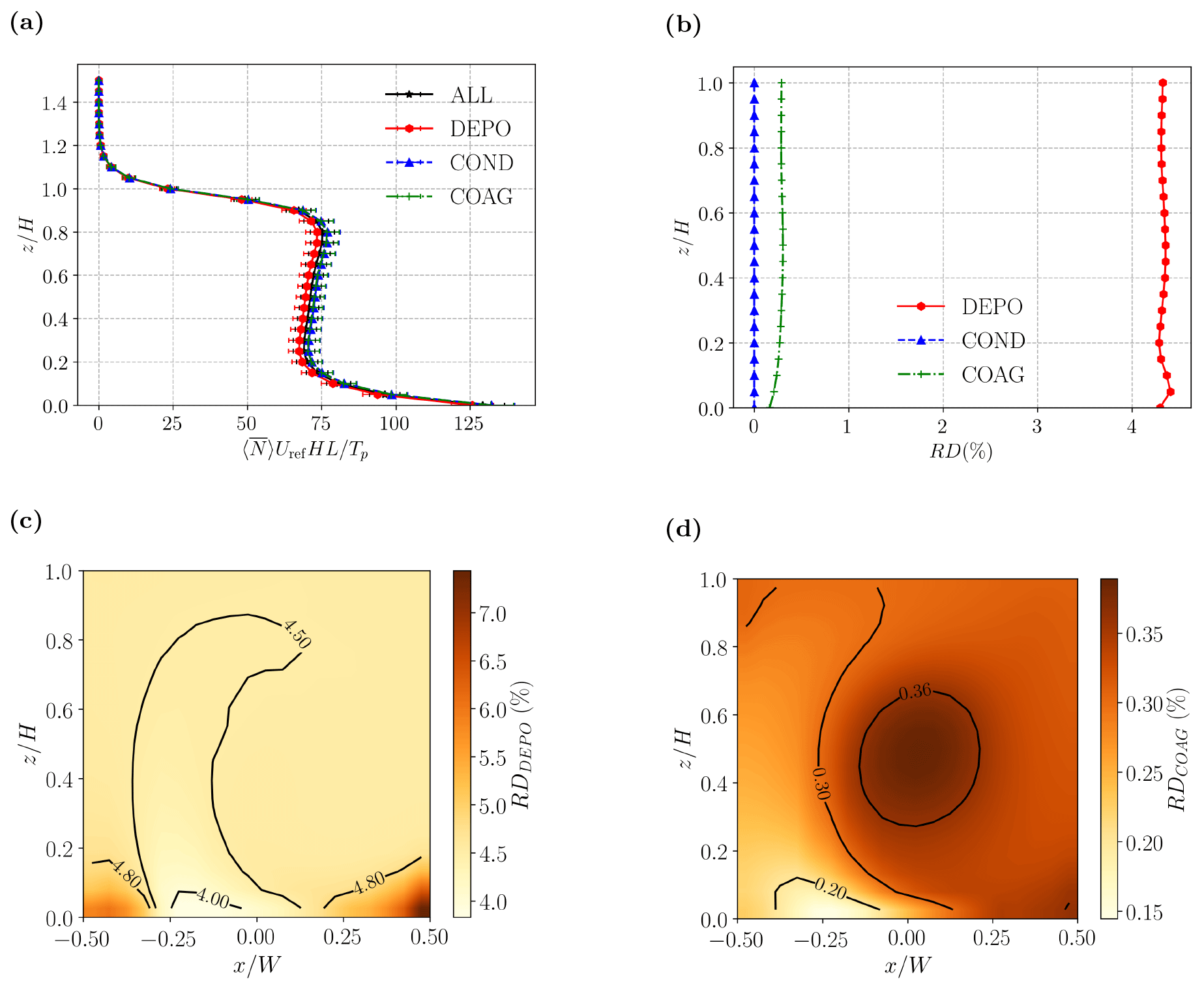
Figure 9 Effect of different aerosol processes for Case TR. Mean vertical profiles of (a) mean aerosol number concentration and (b) relative difference with respect to a simulation without aerosol dynamic processes (NOAD). Spanwise-averaged relative difference fields for (c) deposition and (d) coagulation. The lines correspond to different SALSA configurations (DEPO – deposition only; COND – condensation only; COAG – coagulation only; ALL – deposition, condensation and coagulation).

We now consider the spatial structure of the two most important processes. For deposition (Fig. 9c), RD is maximised in the bottom corners. Values are lower away from the corners, especially near the centreline, $x/W=\mathrm{0}$.

For coagulation (Fig. 9d), by contrast, the pattern is rather different: RD is maximised within the bottom windward vortex and the central canyon vortex. Roughly speaking, the effects of deposition are fairly small outside the bottom corner vortices, while those of coagulation tend to increase away from the source centred at $x/W=\mathrm{0}$. The increase follows the orientation of the mean circulation (see Fig. 2a).

Figure 10 As in Fig. 9 but for Case NG-D.

Figure 11 As in Fig. 9 but for Case CO-D.

3.3.2 Near-ground cooking emissions

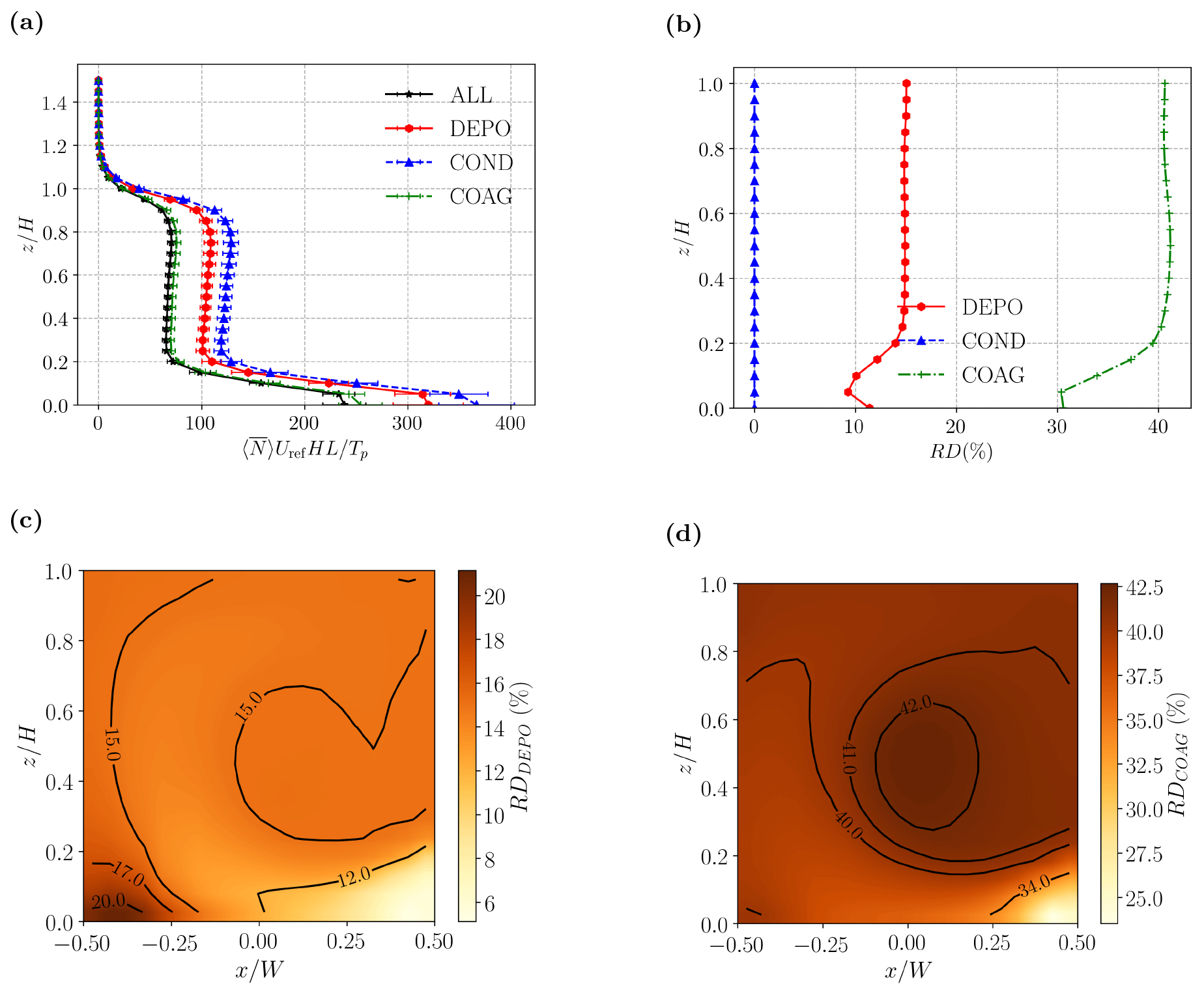
The effects of the different aerosol processes for near-ground deep-frying are compared in Fig. 10. Compared with traffic emissions, the effects of coagulation are much more important: the vertical profiles for COAG and ALL nearly coincide (Fig. 10a), and RD_COAG reaches a maximum of around 40 % (Fig. 10b), which is around 400 times higher than that for traffic emissions. RD_DEPO also increases significantly.

There are several reasons for these differences. First, coagulation occurs more efficiently for particles with D_p<50 nm (Kokkola et al., 2008). Such particles are favoured by the emission spectrum (93 % of the particles generated by deep-frying fall in this category but just 58 % for traffic; Fig. 3). Second, the efficiency of Brownian diffusion increases for smaller particles, leading to higher deposition velocities and enhanced deposition (Zhang et al., 2001; Kurppa et al., 2019). Above $z/H\sim \mathrm{0.2}$, which lies above the corner vortices in Fig. 2, the RD profiles are nearly independent of height.

The spatial structure of the RD fields also changes. For deposition (Fig. 10c), RD is maximised in the bottom leeward corner, while the lowest values are found in the bottom windward corner. (RD gives an exaggerated impression of the absolute difference between the corners as the total number concentration for NOAD is approximately 50 % higher in the windward corner.) For coagulation (Fig. 10d), the lowest values are no longer found around the source centred at $x/W=\mathrm{0}$, as is the case for traffic (Fig. 9d), but rather around the roadside kitchens on the windward wall. Once again, there is indication that the relative importance of coagulation increases away from the source following the sense of the mean circulation. The largest RD values are found near the centre.

Qualitatively similar results are obtained for Case NG-B (Fig. S2). While number concentrations and RD values are lower (cf. Table 2), the structure of the RD fields is largely unchanged from Fig. 10.

3.3.3 Column cooking emissions

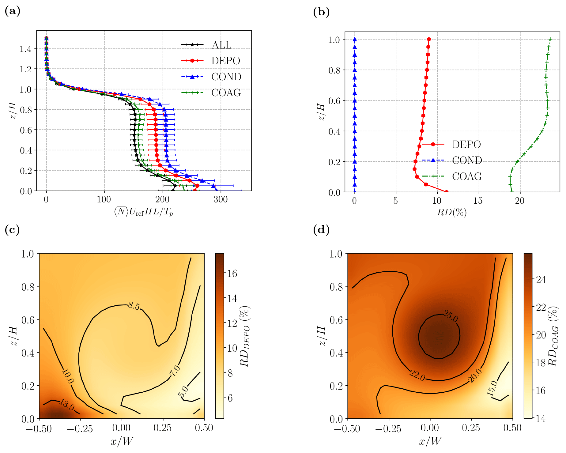
The effects of the different aerosol processes for column deep-frying are compared in Fig. 11.

Although the emission spectrum is unchanged from Case NG-D (Fig. 10), both RD_DEPO and especially RD_COAG decrease (Fig. 11b). This change cannot be directly attributed to the increase in the canyon-averaged number concentration (Table 2). Everything else being the same, the deposition rate should scale linearly with $\stackrel{\mathrm{‾}}{N}$ (Sect. A1), while the coagulation should scale quadratically (Sect. A2). Given the nondimensionalisation and the increase in $\stackrel{\mathrm{‾}}{N}$, one would naively expect RD_DEPO to be approximately unchanged and RD_COAG to increase. Evidently the change in the source configuration, rather than the associated increase in number concentration, is of primary importance. The spatial distribution provides partial insight into this. Analogously to NG-D, RD_DEPO and RD_COAG have relatively low values along the windward wall (Fig. 11c, d); however, the column source covers a larger area, and a plume-like structure (i.e. the tongue of low RD values between the canyon centre and the windward wall) develops away from it. Results for CO-B are qualitatively similar (Fig. S3).

Figure 12 Canyon-averaged aerosol number size distributions for different emission scenarios: (a) traffic; (b) near-ground deep-frying; (c) near-ground boiling; (d) column deep-frying; (e) column boiling. Each line corresponds to a different set of aerosol processes (see Fig. 9 for definitions). The standard error (obtained from the temporal standard deviation) is denoted by the error bars.

3.4 Aerosol number distributions

Aerosol size distributions for ground-level traffic and near-ground cooking are compared in Fig. 12 for different emission scenarios and SALSA configurations. The statistics are evaluated over the entire canyon. Deviations with respect to NOAD reflect the influence of aerosol processes. For Case TR (Fig. 12a), deposition decreases the number of particles in each size bin for D_p<50 nm but has a minimal effect for larger particles. The shape is not exactly preserved because deposition is size-dependent (see Sect. A1). The size spectra for COAG and NOAD are almost identical. The effect of coagulation on the size spectra is more obvious for cooking emissions. For Case NG-D (Fig. 12b), the COAG and ALL spectra are nearly identical; the DEPO concentrations are higher at small scales, D_p<40 nm. For Case NG-B (Fig. 12c), the pattern is similar. The effects of COAG are largest for small particles on account of the emission spectra and the increase in coagulation efficiency for smaller particles.

Similar results are obtained for column emissions. For Case CO-D (Fig. 12d), differences with respect to NOAD are smaller, in agreement with the canyon-averaged concentrations, but compared to NG-D, the range over which coagulation is strongest narrows to D_p≤30 nm. For Case CO-B (Fig. 12e), coagulation leads to decreased concentrations for small particles (D_p<20 nm), as with NG-B.

The uncertainty in the estimate of the time-averaged size distributions is indicated with the (temporal) standard error. Errors are much smaller for the deep-frying cases, NG-D and CO-D. A plausible explanation is that temporal intermittency is greater for cases in which deposition plays a more important role, namely TR, NG-B and CO-B, because deposition only occurs near surfaces and is maximised inside the corner vortices. Coagulation, by contrast, occurs everywhere.

Figure 13 Comparison of characteristic timescales for NG-D. (a) v_d (or $\mathrm{\Delta }/{\mathit{\tau }}_{\text{d}}$); (b) τ_coag.

4 Analysis of the aerosol processes

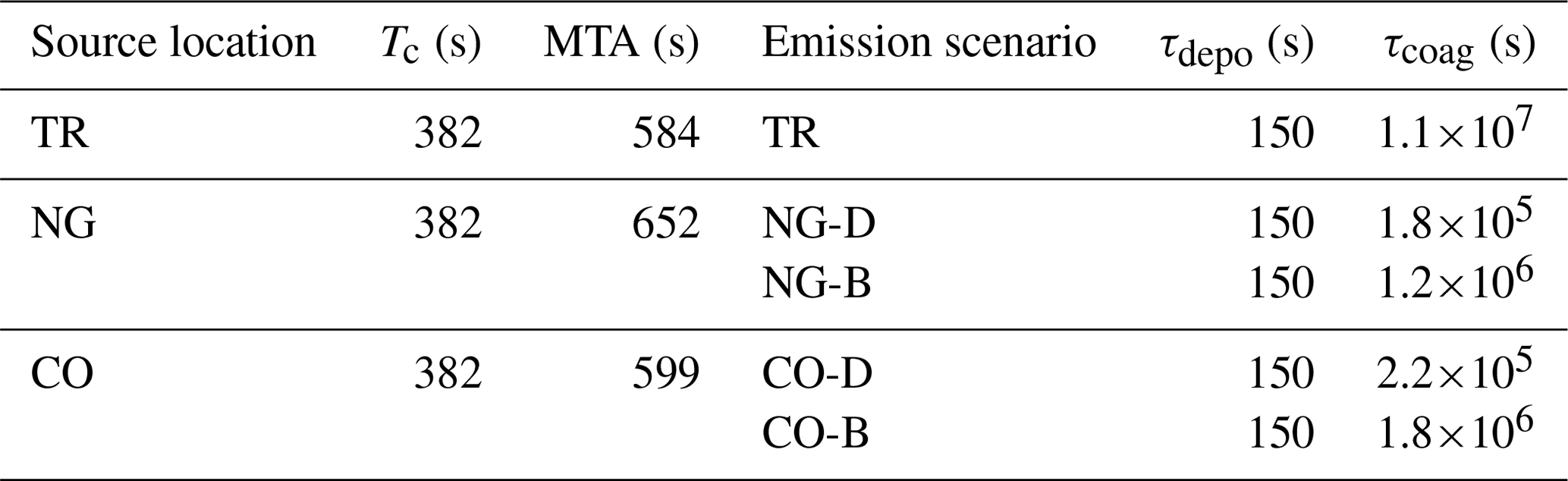
4.1 Characteristic timescales

The differences between the aerosol processes can be understood by referring to the characteristic timescales (Fig. 13). For concreteness, we focus on NG-D. The deposition timescale is derived from the deposition velocity, Eq. (A1a), which is $O\left({\mathrm{10}}^{-\mathrm{2}}\right)\mathrm{m}{\mathrm{s}}^{-\mathrm{1}}$. Hence the deposition timescale for the smallest resolved scale, ${\mathit{\tau }}_{\text{depo}}=\mathrm{\Delta }/v_{\text{d}}\sim \mathrm{150}$ s, while for the corner vortices, τ_depo=O(500) s. Following Ketzel and Berkowicz (2004), the coagulation timescale,

$$\begin{array}{}\text{(3)}& {\displaystyle }{\mathit{\tau }}_{\text{coag}}=N/{\displaystyle \frac{\partial N}{\partial t}}{|}_{\text{coag}},\end{array}$$

may be diagnosed from the evolution equation,

$$\begin{array}{}\text{(4)}& {\displaystyle \frac{\partial N}{\partial t}}{\mid }_{\text{coag}}={\displaystyle \frac{\mathrm{1}}{\mathrm{2}}}\sum _{j=\mathrm{1}}^{k-\mathrm{1}}{\mathit{\beta }}_{k-j,j}{n}_{k-j}{n}_j-\sum _{j=\mathrm{1}}^{\mathrm{\infty }}{\mathit{\beta }}_{k,j}{n}_k{n}_j\end{array}$$

where β_ij is the coagulation kernel. Although this neglects the actual time discretisation (Sect. A2), the error should be negligible so long as Δt≪τ_coag. Using the same β_ij as SALSA and ${\stackrel{\mathrm{‾}}{n}}_i$, the time-averaged number concentrations τ_coag are ∼50 000–500 000 s for NG-D (Fig. 13b). However, this estimate is somewhat misleading because τ_coag is not constant. From integration of Eq. (4), the total number concentration actually decreases from its initial value (i.e. the time-averaged n_i) by a factor of e after ∼1000 s (not shown).

Given these estimates for τ_depo and τ_coag, several predictions about deposition and coagulation can be made. Deposition will preferentially occur where particles can remain close to solid surfaces for an extended duration; the corner vortices are good candidates because particles may be brought near the walls as they recirculate. This is consistent with RD_DEPO (Fig. 10b). Away from the walls, τ_depo is not uniform in the interior because particles are mixed with ambient fluid. The aerosol timescales may be compared to the mean circulation timescale, i.e. $T_{\text{c}}\equiv \mathrm{2}(H/W+U/W)=\mathrm{382}$ s, where U and W are characteristic streamwise and vertical speeds, which yields a good estimate of the mean residence time of pollutants within the canyon (Lo and Ngan, 2017). Since τ_depo≲T_c, deposition is partially but not completely independent of the mean canyon motion; thus deposition does not occur immediately. By contrast, τ_coag≫T_c so that coagulation within the canyon proceeds while particles are being advected and mixed. One therefore expects the structure of RD_COAG to resemble that of the steady passive scalar field (compare Figs. 6c and 9d). More precisely, RD_COAG should be correlated with the age of fluid parcels or the time elapsed between the release of a particle at the source and its arrival at a receptor point. Physically, RD_COAG increases away from the source (i.e. as the age increases) because there is more time for coagulation to occur.

Similar considerations apply to other emission scenarios. For NG-B, v_d is comparable τ_coag∼100 000–500 000 s (with an e-folding time of 7000 s). The implication is that the spatial structure of RD_DEPO and RD_COAG should be largely unchanged. Deposition is strongly affected by the emission spectrum (see Fig. 12), but it should continue to be maximised in the same places for identical flow and source location. Coagulation is much slower compared to NG-D and RD_COAG reduced, but the basic pattern should be unchanged so long as coagulation is a relatively slow process governed by the age along fluid trajectories. These predictions are consistent with Fig. S2. For CO-B, v_d and τ_coag change little from NG-B (by 3.1 % and 4.0 %). As before, one expects deposition to increase within the corner vortices, though the effect on RD_DEPO should be less noticeable within the windward vortex, where concentrations are higher around the source (Fig. 7c). Coagulation should decrease for CO-B on account of the shorter mean ages associated with elevated source locations (see Sect. 4.2).

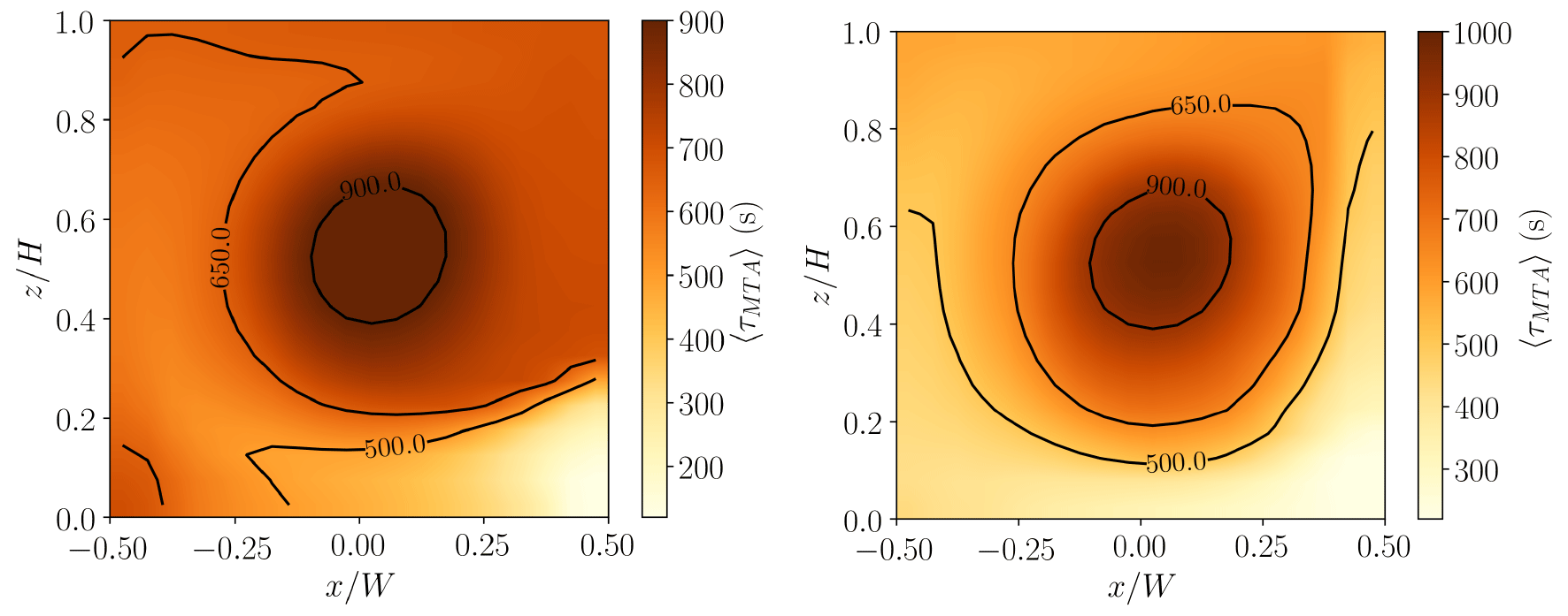
Figure 14 Spanwise-averaged MTA for (a) near-ground and (b) column source. The canyon-averaged MTAs are similar (652 s for the NG source and 599 s for the CO source); however, the spatial structures are noticeably different.

4.2 Mean tracer age

To test these predictions, the age may be calculated by tracking fluid parcels. The mean tracer age Lo and Ngan (MTA; 2015) characterises the average time elapsed between the release of a pollutant at the source and its arrival at the receptor. This is a more appropriate dynamical timescale for coagulation. Following the procedure reviewed in Appendix E, the MTA is calculated for a near-ground source (Fig. 14a). The MTA is lowest near the source at the bottom windward corner and increases towards the centre of the domain, where there are very high values. This pattern is seen most clearly in RD_COAG (Fig. 10d) and, to a lesser extent, RD_ALL (not shown). Linear correlation coefficients between the MTA and the relative difference for NG-D confirm that coagulation is strongly dependent on the age (Table 4). The correlation is weaker for deposition because the MTA is not maximised around the leeward corner. The magnitude of the correlation with RD_DEPO is comparable to that with the total number concentration (not shown), which tends to decrease away from the source. For a column source (Fig. 14b), the correlation between the MTA and the relative differences is comparable.

Table 4 Linear correlations between the relative differences and the MTAs for NG-D and CO-B.

The preceding results imply that resolving the transient dynamics is potentially important for accurate simulation of aerosol dynamical processes. Since coagulation is nonlinear in the concentration and the concentration evolves between the source and receptor, approximating the coagulation term with a time average will introduce errors. These errors could be significant when coagulation is strong, such as is the case for cooking emissions.

The dynamical and aerosol timescales are summarised in Table 5. In all cases, ${\mathit{\tau }}_{\text{depo}}/T_{\text{c}}\mathit{\lesssim }\mathrm{1}$ and ${\mathit{\tau }}_{\text{coag}}/\text{MTA}\gg \mathrm{1}$.

Table 5 Dynamical and aerosol timescales for different emission scenarios.

5 Sensitivity tests

5.1 Background concentrations

The calculations described in Sect. 3 neglect background concentrations, i.e. N_b=0. Although N_b is fixed, the background is still involved in aerosol processes. To assess the effect of the background on the aerosol processes, several cases with N_b>0 are considered.

1. Idealised background spectrum. Here it is assumed that the background spectrum is identical to the emission spectrum. Using a single emission scenario, NG-B, two cases are considered: (i) light pollution, N_b=0.1N₀; (ii) heavy pollution, N_b=0.4N₀, where N₀ is the mean canyon-averaged number concentration for N_b=0. These values are arbitrary; however, the increase in N_b is meant to capture the contrast between normal conditions and a severe pollution episode.

2. Realistic urban background spectrum. Here NG-B is applied to the background spectrum from a real urban measurement (Fig. 15d). The measurement was taken in Tsuen Wan, Hong Kong (see Appendix G for details). The measured spectrum resembles the emission spectrum for traffic (Fig. 3). The measurements suggest N_b=0.5N₀.

Figure 15 Spanwise-averaged relative difference fields of aerosol dynamical processes (ALL). (a) Light pollution; (b) heavy pollution; (c) realistic case; (d) aerosol number size distributions for background concentration (black line) and total concentration (blue line).

Table 6 Canyon-averaged RD_ALL for NG-B and different background cases. Note that the baseline concentration (N_b=0) is identical for idealised and realistic cases.

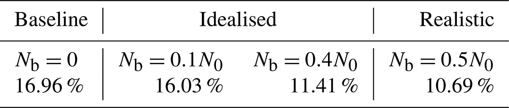
Spatially uniform, constant background concentrations are prescribed over the entire computational domain. The effect of the background is assessed by calculating RD_ALL for different N_b. Note that the background is allowed to interact with the emissions through heterogeneous coagulation. For the idealised cases, RD_ALL decreases as the background concentration is increased to N_b=0.1N₀ and N_b=0.4N₀ (Table 6); for the realistic case, RD_ALL decreases by up to 37 % from its value for N_b=0. Nevertheless, the actual impact is smaller than it may appear on first glance. In the absence of any additional aerosol processes, e.g. if the background were completely inert, RD_ALL would also decrease from the accompanying increase in the total number concentration, N: for N_b=0.1N₀, 0.4N₀ and 0.5N₀, the decreases would be 15.4 %, 12.1 % and 11.3 %, respectively. On account of aerosol processes involving the background only or the background and emissions, the values in Table 6 depart from the crude linear scaling, but the deviations are small, i.e. ∼5 %. The qualitative similarity of the RD_ALL fields (Fig. 15a–c) suggests that the physical mechanisms described in Sect. 4 are robust. This is true even though the simulated size distribution shifts towards large particles when the realistic background spectrum is used (Fig. 15d).

The effect of the background on N is relatively small because N_b is fixed. Hence aerosol processes involving the background do not change N directly: the background affects N only indirectly through the emissions. For example, coagulation between the background and emissions will change the size distribution of the nominal emissions (i.e. the “perturbation” or N−N_b), which will in turn affect the deposition and coagulation rates. This is clearly a nonlinear process.

5.2 Source flux

The dependence on the source flux is usually ignored in studies of pollutant dispersion. For a passive scalar emitted by a uniform source, the concentration scales linearly with the source flux, and this dependence can be removed by the nondimensionalisation, Eq. (1). For aerosols, however, this is no longer true because coagulation depends nonlinearly on the number concentration. This is potentially important because cooking emissions are not constant with time. Here we assess the sensitivity to the source flux Q for Case CO-B. Letting the original source flux be denoted by Q₀, we now consider Q=αQ₀ for $\mathit{\alpha }\in [\mathrm{0.1},\mathrm{10}]$.

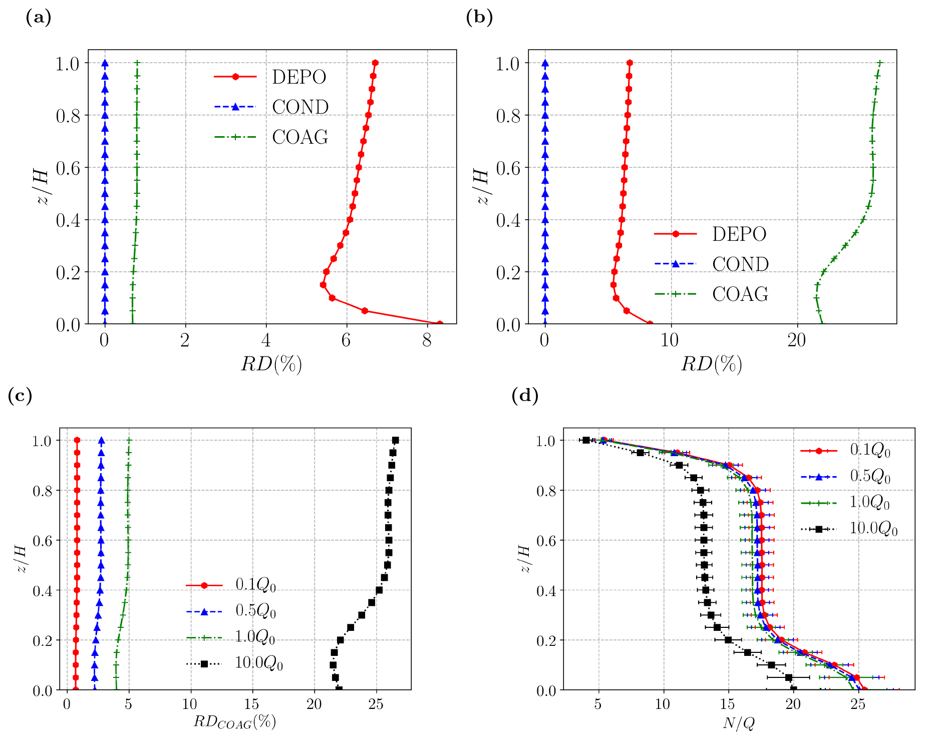
Figure 16 Comparison of aerosol processes and source fluxes, Q, for Case CO-B: panels (a) and (b) compare vertical profiles of RD_i at fixed Q; panels (c) and (d) compare the effect of different Q on coagulation. (a) Q=0.1Q₀; (b) Q=10Q₀; (c) RD_COAG; (d) normalised number concentration, $N/Q$.

The effect on the different aerosol processes is illustrated by vertical profiles of RD_i. For Q=0.1Q₀ (Fig. 16a) and Q=10Q₀ (Fig. 16b), condensation is negligibly small. Deposition also shows weak sensitivity to the source flux as RD_DEPO∼8 % despite the 100-fold increase in Q. However, coagulation shows strong sensitivity to Q₀: it is small for Q=0.1Q₀ (RD_COAG∼0.5 %) but of major importance for Q=10Q₀ (RD_COAG∼25 %). Examining RD_COAG separately (Fig. 16c), the sensitivity is fairly weak for $Q/Q_{\mathrm{0}}\le \mathrm{1}$.

The preceding results may be explained as follows. The dry deposition flux for size bin i is linearly proportional to the concentration, i.e. $F_{\mathrm{d},i}=-v_{\text{d}}{n}_i$, where v_d is the deposition velocity (Seinfeld and Pandis, 2016). The number concentration is directly proportional to Q, but this dependence disappears from RD_DEPO after the nondimensionalisation.

The corresponding coagulation flux (i.e. the contribution of coagulation to the time evolution of n_i) is quadratic in n_i, implying that coagulation should depend sensitively on the source flux. This is partially confirmed by vertical profiles of the normalised concentration, $N/Q$ (Fig. 16d), which suggest a nonlinear dependence on Q for $Q/Q_{\mathrm{0}}>\mathrm{1}$.

6 Discussion

This study has focused on an idealised flow and a small number of representative emission scenarios in order to highlight the basic processes governing the dynamics of cooking-generated urban aerosols. We now discuss how the results may extend to more realistic cases.

The emission scenarios defined in Table 1 are arbitrary. Obviously other kitchen dimensions or locations could be chosen, but the results presented here should serve as a starting point for future studies of specific urban environments. The sensitivity to the source flux cannot be strictly neglected, but at least for deviations of ∼50 % from the baseline value, the effect is modest (Fig. 16). The qualitative response to the source location can be estimated from the behaviour for a passive scalar as the inclusion of aerosol processes has little effect on spatial structure of the number concentration fields (e.g. Fig. 1b). Although the results inevitably depend on the emission spectrum – mean concentrations for boiling and deep-frying differ by ∼30 % for near-ground emissions and ∼15 % for column emissions (Table 2) – there is no evidence for strong sensitivity. Test calculations in which the emission spectrum for NG-B is scaled by a factor of 2 or 0.5 show limited sensitivity. For example, the vertical profiles show a nearly identical shape with mean concentrations differing by less than 5 % with respect to the default emission spectrum (Fig. S4). Furthermore, the spatial structure of the relative difference fields is almost identical (Fig. S5).

Flow over a unit-aspect-ratio street canyon has been a benchmark case for examining urban air quality chemistry (Zhong et al., 2015) because it captures the effects of decreased ventilation or, equivalently, a finite residence time for chemical reaction (Harrison, 2018). The analysis of Sect. 4 implies that the spatial structure of deposition and coagulation is determined primarily by two factors: the streamline geometry or mean circulation and the ratio of the aerosol and dynamical timescales. Deposition is promoted when particles are brought into repeated contact with solid surfaces, such as occurs within corner vortices. Coagulation requires the ageing of pollutants, which occurs along fluid trajectories in the outdoor environment. Hence the nature of the aerosol dynamics for a given emission spectrum should depend on the ratio of the aerosol timescales to the dynamical timescales, at least for relatively small perturbations in which the streamline geometry is maintained. This is a variant of the argument that the nature of urban gas-phase chemistry is strongly influenced by the ratio of the chemical timescale to the residence time (Harrison, 2018).

With other emission scenarios or flows, quantitative differences are unavoidable, but qualitative differences in the aerosol dynamics are not expected in most cases. For cooking emissions, the coagulation timescale is much longer than the relevant dynamical timescale (Table 5), which implies that coagulation will continue to be controlled by the ageing of fluid parcels or the mean tracer age. The dynamical timescales change with the wind direction (Table S1), but the coagulation timescale, τ_coag, remains much longer. For stratified flow, the MTA will decrease for unstable stratification and increase for stable stratification, but the effect should be relatively small (see Duan and Ngan, 2019 for building array results). The situation is more complicated for deposition insofar as τ_depo is not much less than the relevant dynamical timescale, i.e. the canyon circulation timescale T_c. Qualitatively different behaviour is expected only for a much smaller T_c, such as may occur for unstable flow or a street canyon with lateral openings. In this case, deposition will be less spatially localised and will no longer proceed to completion. For cooking emissions, the relative contribution of deposition would therefore decrease compared to the cases examined in this paper, for which ${\mathit{\tau }}_{\text{depo}}/T_{\text{c}}<\mathrm{1}$.

A highly simplified representation of indoor aerosol processes was adopted. Since details of the kitchen ventilation systems and exhaust ducts vary, we focused on a configuration in which indoor aerosol processes and the effects of the ventilation system are ignored: it is assumed that all cooking-generated particles escape without loss, modification or re-entrainment. The results described in this study therefore correspond to an idealised but important limit. Given the fairly weak sensitivity to source flux and source location, one may expect that the results will not be greatly affected by the indoor aerosol processes unless there is a significant change in the emission strength or spectrum. The characteristic timescales for the outdoor aerosol processes (Fig. 13) suggest that the effects of indoor coagulation and deposition could be relatively weak; however, detailed analysis of ventilation systems would be required to quantify the effect. Calculations including an urban background derived from real urban measurements show that the spatial structure of the aerosol processes is essentially independent of the background spectrum. Moreover, the quantitative effect on the relative differences is small compared to the change in the total particle number.

The assumptions described above may partially explain why the mass concentrations (Appendix D) are very high. For example, concentrations would decrease if the assumption of perfect ventilation to the exterior were relaxed.

7 Conclusions

Cooking-generated aerosols differ significantly from traffic-generated ones. Using standard emission spectra and plausible assumptions about the traffic volume and restaurant dimensions, it was found that the number concentration within a unit-aspect-ratio street canyon is ∼50 %–100 % higher for boiling and deep-frying than for traffic. This reflects differences in the emission factors and the increased importance of deposition and coagulation: whereas the inclusion of deposition or coagulation for traffic emissions leads to changes of around 4.5 % and 0.4 %, respectively, relative differences of 15.3 % and 41.3 % are found for near-ground deep-frying. Coagulation is especially important for deep-frying, which generates many small particles with diameter D_p<50 nm. The results support the finding that organic aerosols may be determined primarily by cooking emissions in neighbourhoods with many restaurants (Lee et al., 2015; Liu et al., 2018). Even larger differences are seen in the mass concentration, though the effect of aerosol processes on PM_2.5 is much smaller.

The sensitivity of the results to the source spectrum and source location can be understood by analysing the deposition and coagulation timescales. For the different cooking-emission scenarios, both timescales are comparable to or longer than the characteristic timescale for large-scale motions within the canyon. The upshot is that deposition is enhanced within corner vortices while coagulation occurs following fluid trajectories. The mean tracer age, which characterises the ageing of particles released at the source, reveals the spatial structure of coagulation.

The present study is restricted to idealised flow and emission scenarios. It would be instructive to perform a similar study for a real street canyon that contains restaurants. This would enable the impact of assumptions about the kitchen emission factors or the neglect of heated plumes to be assessed. However, in situ measurements, preferably of the size spectrum, would be required.

Appendix A: Aerosol parameterisations

A1 Deposition

Dry deposition occurs when particles impact and stick to a solid surface. Many schemes have been developed for calculating the dry deposition velocity, v_d. In SALSA, the scheme of Zhang et al. (2001) is applied:

$$\begin{array}{}\text{(A1a)}& {\displaystyle }{v}_{\text{d}}& {\displaystyle }=v_g+{\displaystyle \frac{\mathrm{1}}{R_{\text{a}}+R_{\text{s}}}},\text{(A1b)}& {\displaystyle }{u}_g& {\displaystyle }={\displaystyle \frac{\mathit{\rho }{d}_p^{\mathrm{2}}gC}{\mathrm{18}\mathit{\eta }}},\text{(A1c)}& {\displaystyle }{R}_{\text{a}}& {\displaystyle }={\displaystyle \frac{\ln z_R/z_{\mathrm{0}}-{\mathit{\psi }}_H}{\mathit{\kappa }{u}_{*}}},\text{(A1d)}& {\displaystyle \frac{\mathrm{1}}{R_{\text{s}}}}& {\displaystyle }={\mathit{\epsilon }}_{\mathrm{0}}{u}_{*}\left(S{c}^{-\mathit{\gamma }}+{\left({\displaystyle \frac{St}{\mathrm{0.8}+St}}\right)}^{\mathrm{2}}+{\displaystyle \frac{\mathrm{1}}{\mathrm{2}}}{\left({\displaystyle \frac{d_p}{A}}\right)}^{\mathrm{2}}\right)R_{\mathrm{1}},\end{array}$$

where v_g is the gravitational settling velocity; R_a and R_s represent the aerodynamic resistance and surface resistance, respectively; ρ is the particle density; g is the acceleration of gravity; η is the viscosity; and C is a correction factor. In Eq. (A1c), z_R is the height, z₀ is the roughness length, u_* is the friction velocity, ψ_H is the stability function, and κ is the von Karman constant. For LES, u_* is estimated by $\sqrt{C_d}U$, where C_d is the drag coefficient and U is the local velocity magnitude. Sc is the particle Schmidt number and St is the Stokes number. ε₀, γ and A are constants based on the surface type.

A2 Coagulation

Coagulation occurs when two particles collide and form a larger one. Following Jacobson and Jacobson (2005), the number concentration for size bin i is given by

$$\begin{array}{}\text{(A2)}& n_{i,t}={\displaystyle \frac{n_{i,t-\mathrm{\Delta }t}+\frac{\mathrm{1}}{\mathrm{2}}\mathrm{\Delta }t{\sum }_{j=\mathrm{1}}^{i-\mathrm{1}}{\mathit{\beta }}_{i-j}{n}_{i-j}{n}_{j,t-\mathrm{\Delta }t}}{\mathrm{1}+\mathrm{\Delta }t{\sum }_{j=\mathrm{1}}^{\mathrm{\infty }}{\mathit{\beta }}_{i,j}{n}_{j,t-\mathrm{\Delta }t}}},\end{array}$$

where δ_t is the time step and β represents the coagulation kernel (cm³ per particle per second) for particles in size bins i and j. The coagulation kernel or rate coefficient is calculated as

$$\begin{array}{}\text{(A3)}& {\mathit{\beta }}_{i,j}={\displaystyle \frac{\mathrm{4}\mathit{\pi }(r_i+r_j)(D_i+D_j)}{\frac{r_i+r_j}{r_i+r_j+({\mathit{\delta }}_i^{\mathrm{2}}+{\mathit{\delta }}_j^{\mathrm{2}}{)}^{\mathrm{1}/\mathrm{2}}}+\frac{\mathrm{4}(D_i+D_j)}{({\stackrel{\mathrm{‾}}{{\mathit{\nu }}_{pi}}}^{\mathrm{2}}+{\stackrel{\mathrm{‾}}{{\mathit{\nu }}_{pj}}}^{\mathrm{2}}{)}^{\mathrm{1}/\mathrm{2}}(r_i+r_j)}}}.\end{array}$$

Here, D is the particle diffusion coefficient; δ denotes the mean distance from the centre of a sphere defined by the particle mean free path, λ_pi; $\stackrel{\mathrm{‾}}{{\mathit{\nu }}_p}$ is the thermal velocity.

A3 Condensation

Condensation increases the particle volume through mass transfer. Following Jacobson and Jacobson (2005), the vapour mole concentration of a condensing gas g is calculated as

$$\begin{array}{}\text{(A4)}& \begin{array}{rl}& C_{g,t}=\\ & {\displaystyle \frac{C_{g,t-\mathrm{\Delta }t}+\mathrm{\Delta }t{\sum }_{i=\mathrm{1}}^N\left(k_{g,i,t-\mathrm{\Delta }t}{S}_{g,i,t-\mathrm{\Delta }t}^{\prime }{C}_{g,s,i,t-\mathrm{\Delta }t}\right)}{\mathrm{1}+\mathrm{\Delta }t{\sum }_{i=\mathrm{1}}^N{k}_{g,i,t-\mathrm{\Delta }t}}},\end{array}\end{array}$$

from which the particle mole concentration may be updated,

$$\begin{array}{}\text{(A5)}& \begin{array}{rl}& c_{g,i,t}=c_{g,i,t-\mathrm{\Delta }t}+\mathrm{\Delta }t{k}_{g,i,t-\mathrm{\Delta }t}\\ & \left(C_{g,t}{S}_{g,i,t-\mathrm{\Delta }t}^{\prime }{C}_{g,s,i,t-\mathrm{\Delta }t}\right).\end{array}\end{array}$$

Here, $k_{g,i,t-\mathrm{\Delta }t}$ is the mass-transfer coefficient (s⁻¹), $S_{g,i,t-\mathrm{\Delta }t}^{\prime }$ is the equilibrium saturation ratio and $C_{g,s,i,t-\mathrm{\Delta }t}$ is the uncorrected saturation vapour mole concentration (mol m⁻³).

The equilibrium saturation ratio and the uncorrected saturation vapour mole concentration are calculated as

$$\begin{array}{}\text{(A6a)}& {\displaystyle }& {\displaystyle }{S}_{g,i}^{\prime }=\exp \left({\displaystyle \frac{\mathrm{4}\mathit{\sigma }{m}_i}{D_i{R}^{\ast }T{\mathit{\rho }}_i}}\right)\text{(A6b)}& {\displaystyle }& {\displaystyle }{C}_{g,s,i}=p_{g,s}/R^{\ast }T,\end{array}$$

where σ is the average particle surface tension, m_i is the average particle molecular weight, D_i is the particle diameter, R^∗ is the universal gas constant, T is the temperature, ρ_i is the average particle density and p_g,s is the gas's saturation vapour pressure.

Appendix B: Chemical compositions and emission factors for gaseous compounds

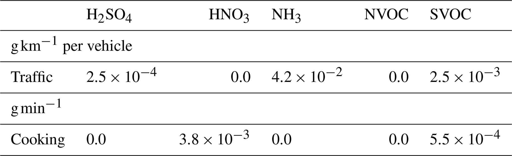
Table B1 Chemical compositions for cooking (See and Balasubramanian, 2008) and traffic (Yubero et al., 2015) emissions. In the former case, a gas stove is assumed.

Table B2 Gaseous emission factors for cooking (Shen et al., 2018) and traffic (Kumar et al., 2008) emissions. In the latter case, the emission factors are derived by assuming that there is one stove for a kitchen of volume 16 m³.

Appendix C: Validation of scalar statistics

Time-averaged concentration statistics are compared with the wind-tunnel data of Pavageau and Schatzmann (1999) by introducing a ground-level line source along the central axis of the unit-aspect-ratio street canyon. The numerical configuration is otherwise unchanged from Sect. 2.3. Figure C1 shows normalised concentration profiles at different streamwise positions. Concentrations are consistently overpredicted at the leeward wall, centre and windward wall; however, the agreement is at least as good as the previous LES validation of Michioka et al. (2011). In order to quantify the agreement, standard air quality metrics (Chang and Hanna, 2004) are calculated:

$$\begin{array}{}\text{(C1)}& {\displaystyle }& {\displaystyle }\mathrm{FB}={\displaystyle \frac{\stackrel{\mathrm{‾}}{C_{\text{o}}}-\stackrel{\mathrm{‾}}{C_{\text{p}}}}{\mathrm{0.5}(\stackrel{\mathrm{‾}}{C_{\text{o}}}+\stackrel{\mathrm{‾}}{C_{\text{p}}})}},\text{(C2)}& {\displaystyle }& {\displaystyle }\mathrm{NMSE}={\displaystyle \frac{\stackrel{\mathrm{‾}}{(C_{\text{o}}-C_{\text{p}}{)}^{\mathrm{2}}}}{\stackrel{\mathrm{‾}}{C_{\text{o}}}\stackrel{\mathrm{‾}}{C_{\text{p}}}}},\end{array}$$

where C_p and C_o denote the model predictions and observations, respectively. A perfect model would have $\mathrm{FB}=\mathrm{NMSE}=\mathrm{0}$. For the validation, NMSE = 0.07 and FB = 0.2, indicating relatively good agreement. We conclude that the model is capable of predicting mean concentrations for a passive scalar within a street canyon.

Figure C1 Vertical profiles of the normalised mean concentration plotted at $x/W=-\mathrm{0.5}$, 0 and 0.5. The results from present LES simulations are plotted in blue lines and are compared with wind-tunnel data from Pavageau and Schatzmann (1999) (red circles) and LES data from Michioka et al. (2011) (green squares). U_2.5H denotes the temporal and spatial average of the streamwise velocity at $z/H$ = 2.5, and Q is the source flux.

Appendix D: Mass concentrations

Mean mass concentration fields for traffic and near-ground emissions are plotted in Fig. D1.

Figure D1 As in Fig. 6 but for PM_2.5 concentrations. The mass concentrations are largely insensitive to aerosol dynamic processes.

Appendix E: Calculation of the mean tracer age

The mean tracer age measures the time elapsed from the release of a passive scalar at a source location to its arrival at the receptor. The theory is described in Holzer and Hall (2000) and Lo and Ngan (2015). Briefly, a Green function, G(x|x₀), which maps the scalar concentration from the source x₀ to the receptor x, is obtained from the solution of the advection–diffusion equation for an impulse source (i.e. delta function in time). The age spectrum or probability distribution, Z, of transit times, ξ, is given by

$$\begin{array}{}\text{(E1)}& Z(\mathbf{x},\mathit{\xi })={\displaystyle \frac{{\int }_{D}G(\mathbf{x},\mathit{\xi }|{\mathbf{x}}_{\mathbf{0}}\left)S\right({\mathbf{x}}_{\mathrm{0}})d{\mathbf{x}}_{\mathrm{0}}}{c(\mathbf{x},t)}},\end{array}$$

where S refers to the source and c is the concentration. The mean tracer age is the first moment of the age spectrum, i.e.

$$\begin{array}{}\text{(E2)}& {\mathit{\tau }}_{\text{MTA}}=\underset{\mathrm{0}}{\overset{\mathrm{\infty }}{\int }}\mathit{\xi }Zd\mathit{\xi }.\end{array}$$

Appendix F: Measurements of the background size spectrum

The measurements were conducted from 1 to 8 March at 13:00–18:00 local time on the roof of Hoi Pa Street Government Primary School, Tsuen Wan, Hong Kong (height: 31 m; coordinates: 22.372^∘ N, 114.115^∘ E; Fig. F1). Using a Kanomax PAMS 3300 spectrometer and 14 fixed channels, the number distribution was measured from 14.51 to 862.32 nm. The number spectra (75 in total) were averaged to yield the spectrum of Fig. 15d. The site is located in a suburban neighbourhood. During the measurement period, the average traffic volume along the main road (Tai Ho Road) was 2050 vehicles h⁻¹. The mean number concentration $\stackrel{\mathrm{‾}}{N}=\mathrm{2.3}\times {\mathrm{10}}^{\mathrm{10}}{\mathrm{m}}^{-\mathrm{3}}$, implying N_b=0.5N₀, where N₀ is the mean canyon-averaged number concentration for NG-B.

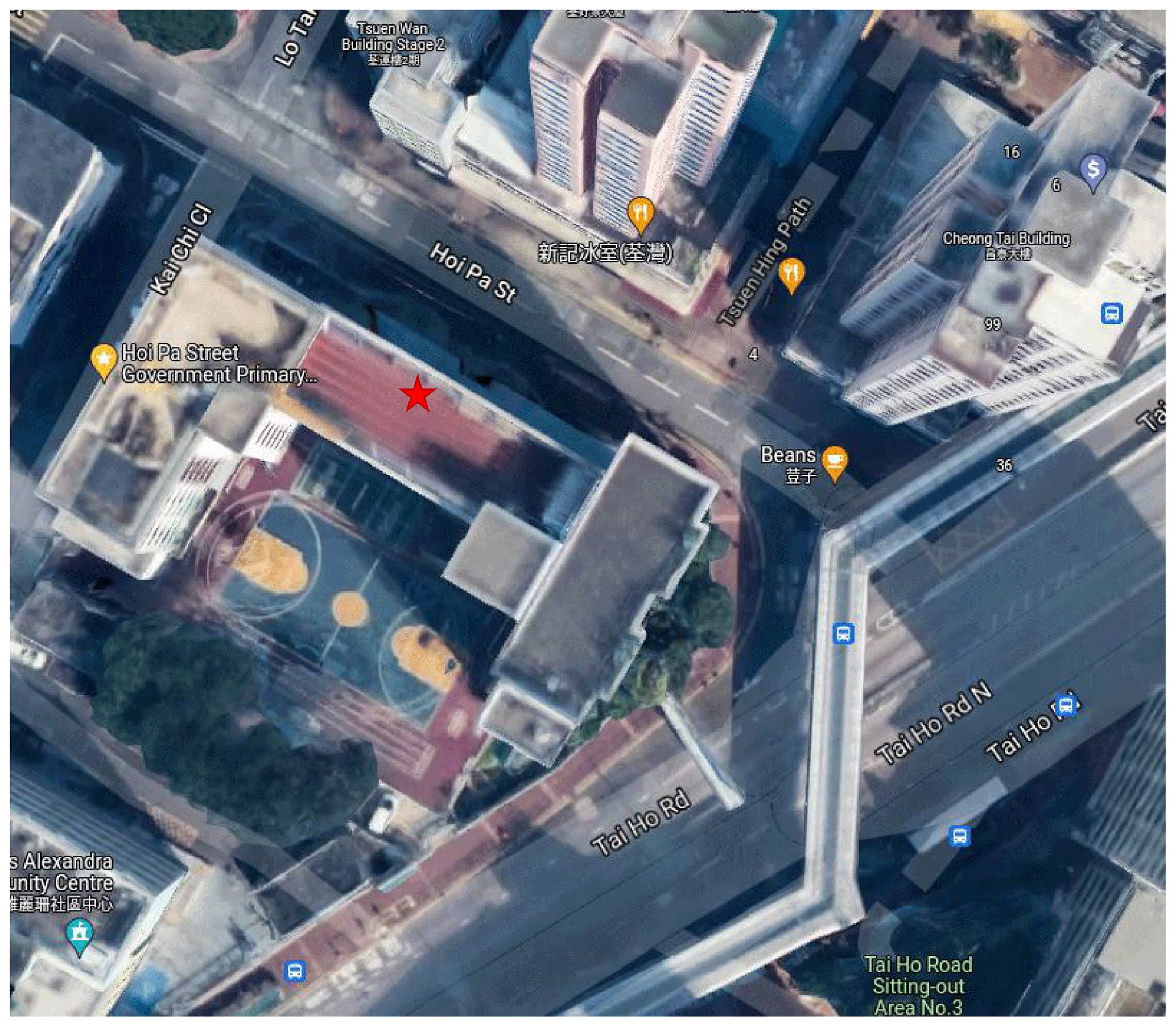
Figure F1 Measurement site in Tsuen Wan, Hong Kong (image taken from © Google Maps). The measurement location is indicated by the red star.