the Creative Commons Attribution 4.0 License.
the Creative Commons Attribution 4.0 License.
 | 11 Feb 2022
Source-resolved variability of fine particulate matter and human exposure in an urban area
Pablo Garcia Rivera
Brian T. Dinkelacker
Ioannis Kioutsioukis
Peter J. Adams
Spyros N. Pandis
Increasing the resolution of chemical transport model (CTM) predictions in urban areas is important to capture sharp spatial gradients in atmospheric pollutant concentrations and better inform air quality and emissions controls policies that protect public health. The chemical transport model PMCAMx (Particulate Matter Comprehensive Air quality Model with Extensions) was used to assess the impact of increasing model resolution on the ability to predict the source-resolved variability and population exposure to PM2.5 at 36×36, 12×12, 4×4, and 1×1 km resolutions over the city of Pittsburgh during typical winter and summer periods (February and July 2017). At the coarse resolution, county-level differences can be observed, while increasing the resolution to 12×12 km resolves the urban–rural gradient. Increasing resolution to 4×4 km resolves large stationary sources such as power plants, and the 1×1 km resolution reveals intra-urban variations and individual roadways within the simulation domain. Regional pollutants that exhibit low spatial variability such as PM2.5 nitrate show modest changes when increasing the resolution beyond 12×12 km. Predominantly local pollutants such as elemental carbon and primary organic aerosol have gradients that can only be resolved at the 1×1 km scale. Contributions from some local sources are enhanced by weighting the average contribution from each source by the population in each grid cell. The average population-weighted PM2.5 concentration does not change significantly with resolution, suggesting that extremely high resolution PM2.5 predictions may not be necessary for effective urban epidemiological analysis at the county level.
- Article
(6884 KB) - Full-text XML
-
Supplement
(1208 KB) - BibTeX
- EndNote


Particulate matter with aerodynamic diameter less than 2.5 µm (PM2.5) contributes to poor air quality throughout large parts of the United States. These particles directly affect visibility (Seinfeld and Pandis, 2006) and have been associated with long- and short-term health effects such as premature death due to cardiovascular disease, increased chance of heart attacks and strokes, and reduced lung development and function in children and people with lung diseases such as asthma (Dockery and Pope, 1994).
At high resolutions, emissions from local sources such as commercial cooking, on-road traffic, residential wood combustion, and industrial activities can have sharp gradients that influence the geographical distribution of PM2.5 concentrations. High-resolution measurements of PM1 have found gradients of up to ∼2 µg m−3 between urban background sites and those with high local emissions (Gu et al., 2018; Robinson et al., 2018).
A key limiting factor on the modeling of particulate matter at high resolutions is the geographical distribution of emissions. Previous studies have found that coarse-grid emissions that are interpolated to higher resolutions lead to small to modest improvements in model predictive ability for ozone (Arunachalam et al., 2006; Kumar and Russell, 1996), secondary organic aerosol (Fountoukis et al., 2013; Stroud et al., 2011), and nitrate (Zakoura and Pandis, 2019, 2018). Pan et al. (2017) used the default approach from the U.S. Environmental Protection Agency (EPA) National Emissions Inventory (NEI) to allocate county-based emissions to model grid cells at 4×4 and 1×1 km and found only small changes to model performance for NOx and O3, while the 1×1 km case showed more detailed features of emissions and concentrations in heavily polluted areas.
Improvements in the resolution of emission inventories have been focused on traffic as this source exhibits significant variability at high resolutions. Recent approaches to building high-resolution traffic inventories include origin–destination by vehicle class (Ma et al., 2020), synthetic population mobility (Elessa Etuman and Coll, 2018), and fuel sales combined with traffic counts (McDonald and McBride, 2014). Other sectors such as biomass burning for residential heating and commercial cooking have been identified as very uncertain in current inventories (Day et al., 2019). Recent versions of the NEI have made progress addressing the total emissions and temporal distributions of biomass burning and commercial cooking (Eyth and Vukovich, 2016), but there is still significant uncertainty on their geographical location at the sub-county scale. Robinson et al. (2018) found greatly elevated organic aerosol concentrations (10s of µg m−3) in the vicinity of numerous individual restaurants and commercial districts containing groups of restaurants indicating that commercial cooking is a source of large gradients on the urban scale.
Population density and socio-economic indicators of that population, such as income or access to healthcare, show large gradients in the urban scale. It is important to assess the exposure of different sub-populations to air pollutants and the resulting health effects, a concept known as environmental justice (Anand, 2002).
We use the Particulate Matter Comprehensive Air quality Model with Extensions (PMCAMx) to study the impact of increasing model resolution on the model's ability to predict the variability, sources, and population exposure of PM2.5 concentrations on the urban scale in Pittsburgh. We compare predicted variability at 36×36, 12×12, 4×4, and 1×1 km resolutions over the city of Pittsburgh during one typical summer and one typical winter month of 2017. Additional sensitivity simulations were performed to determine contributions from selected sources to concentrations. The results of the simulations are used to estimate exposure to PM2.5 at all resolutions and from the selected sources. A detailed evaluation of the PMCAMx predictions against measurements will be the topic of a future publication. Overall the model performance was similar to those in previous model applications in the eastern US (Fountoukis et al., 2013).
The Particulate Matter Comprehensive Air quality Model with Extensions (PMCAMx) (Karydis et al., 2010; Murphy and Pandis, 2009; Tsimpidi et al., 2010) uses the framework of the CAMx model (ENVIRON, 2005) to describe horizontal and vertical advection and diffusion, emissions, wet and dry deposition, and gas-, aqueous- and aerosol-phase chemistry. A sectional approach with 10 size sections is used to dynamically track the evolution of the aerosol mass distribution. The aerosol species modeled include sulfate, nitrate, ammonium, sodium, chloride, elemental carbon, water, primary and secondary organics, and other non-volatile aerosol components. The SAPRC (Statewide Air Pollution Research Center) photochemical mechanism (Carter, 2000) is used for the simulation of gas-phase chemistry. The version of SAPRC used here includes 237 reactions and 91 individual and surrogate species. For inorganic growth, a bulk equilibrium approach was used, assuming equilibrium between the bulk inorganic aerosol and gas phases (Pandis et al., 1993). Aqueous-phase chemistry is simulated using the variable size resolution model (VSRM) (Fahey and Pandis, 2001). The partitioning of the various semivolatile inorganic aerosol components and aerosol water is determined using the ISORROPIA-I aerosol thermodynamics model (Nenes et al., 1998). The primary and secondary organic aerosol components are described using the volatility basis set approach (Donahue et al., 2006). For primary organic aerosol (POA) 10 volatility bins with effective saturation concentrations ranging from 10−3 to 106 µg m−3 at 298 K are used. The volatility distribution for POA from Tsimpidi et al. (2010) was used for all sources, while size distributions are specific to each emission sector. Anthropogenic (aSOA) and biogenic (bSOA) secondary organic aerosol are modeled with four volatility bins (1, 10, 102, 103 µg m−3) (Murphy and Pandis, 2009) using NOx-dependent yields (Lane et al., 2008). Both fine and coarse PM are simulated by PMCAMx, although the following analysis in this work is focused on fine PM. More detailed descriptions of PMCAMx can be found in Fountoukis et al. (2011) and Zakoura and Pandis (2018).
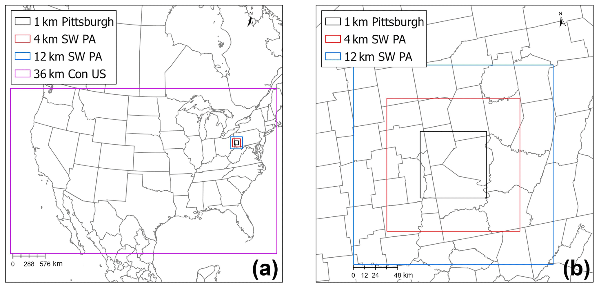
Figure 1Modeling domain used for the PMCAMx simulations. (a) 36×36 km continental US grid. (b) 12×12 and 4×4 km southwestern Pennsylvania grids, as well as 1×1 km Pittsburgh nested grids.
PMCAMx was used to simulate air quality over the metropolitan area of Pittsburgh during February and July 2017. For the base-case simulation we used a one-way nested structure with a 36×36 km master grid covering the continental United States, with nested grids of 12×12 km and 4×4 km in southwestern Pennsylvania and a 1×1 km grid covering the city of Pittsburgh, most of Allegheny County, and the upper Ohio River valley (Fig. 1a). The 1×1 km grid covers a 72×72 km area (Fig. 1b). Two days in each simulation were used for model spin-up and discarded for all analyses. Simulations required approximately 6 CPU days, 5 CPU hours, 10 CPU hours, and 12 CPU days to complete in a single Intel Xeon CPU E5-4640 at 2.4 GHz for the 36, 12, 4, and 1 km domains, respectively.
The surface concentrations at the boundaries of the 36×36 km grid are shown in Table S1 in the Supplement. These values were applied to all upper air layers assuming a constant mixing ratio. Results from lower-resolution simulations were used as boundary conditions for the corresponding next higher-resolution simulation. Horizontal wind components, vertical diffusivity, temperature, pressure, water vapor, clouds, and rainfall were generated using the Weather Research and Forecasting (WRF v3.6.1) Model over the whole modeling domain with horizontal resolution of 12 km. The data were interpolated to higher resolutions when needed. The interpolation of meteorological fields from 12×12 km to higher resolutions is a potential limitation of this work and will be the focus of future improvements to the modeling methods. Initial and boundary meteorological conditions for the WRF simulations were generated from the ERA-Interim global climate re-analysis database, together with the terrestrial data sets for terrain height, land use, soil categories, etc. from the United States Geological Survey (USGS) database. The WRF modeling system was prepared and configured in a similar way as described by Gilliam and Pleim (2010). This configuration is recommended for air quality simulations (Hogrefe et al., 2015; Rogers et al., 2013). A total of 28 vertical layers were used in the WRF simulations to produce 14 layers of meteorological input for the PMCAMx simulations. Each of the 14 PMCAMx layers corresponds to a WRF layer.
Emissions were calculated using the EPA's emission modeling platform (v6.3) for the National Emissions Inventory for 2011 (NEI11) (Eyth and Vukovich, 2016) using the default 2017 projected values. Base emissions were calculated first at a 12 km resolution for the full modeling domain using the Sparse Matrix Operator Kernel Emissions (SMOKE) model and our WRF meteorological data. The data sources used to produce 12 km resolution surrogates with platform v6.3 were used to develop surrogates at 4×4 and 1×1 km resolution for all sectors except commercial cooking and on-road traffic for which custom surrogates were developed. These custom surrogates also use projected values for 2017. Bicubic interpolation was used to produce biogenic emissions at 4×4 and 1×1 km resolution, in areas in which sufficient data were unavailable. The emissions by all sources together with the chemical composition are summarized in Tables 1 (for the winter period) and 2 (for the summer period).
Table 1PM2.5 emissions by source for the 1×1 km Pittsburgh domain (February 2017).
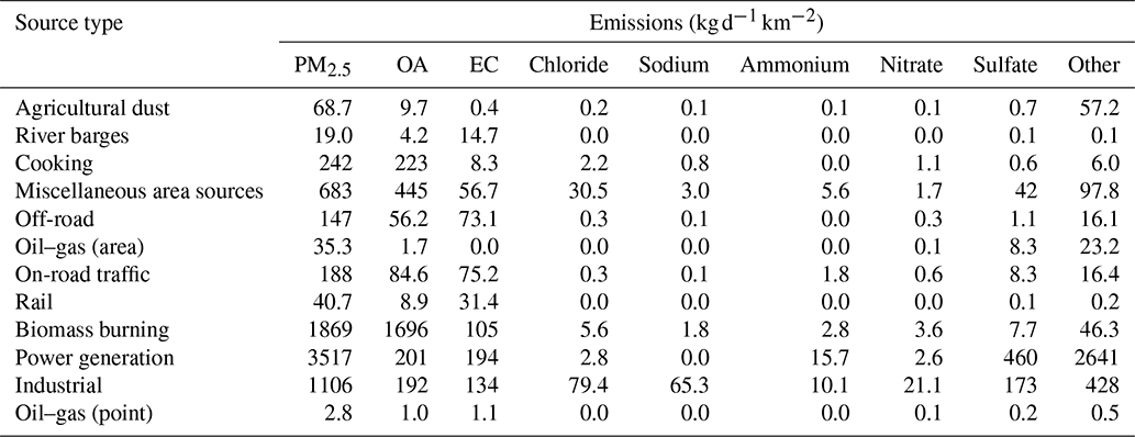
Table 2PM2.5 emissions by source for the 1×1 km Pittsburgh domain (July 2017).

In this work, we used normalized restaurant count to distribute the commercial cooking emissions in space in the 1×1 and 4×4 km resolution domains. Geographical information was collected for all locations labeled as “restaurant” from the freely accessible Google Places application programming interface (API) for the western Pennsylvania area, eastern Ohio, and northern West Virginia. Using this new spatial surrogate, PM2.5 emissions from commercial cooking are enhanced primarily in the Pittsburgh urban core with a maximum increase of 1200 (Fig. 2a).
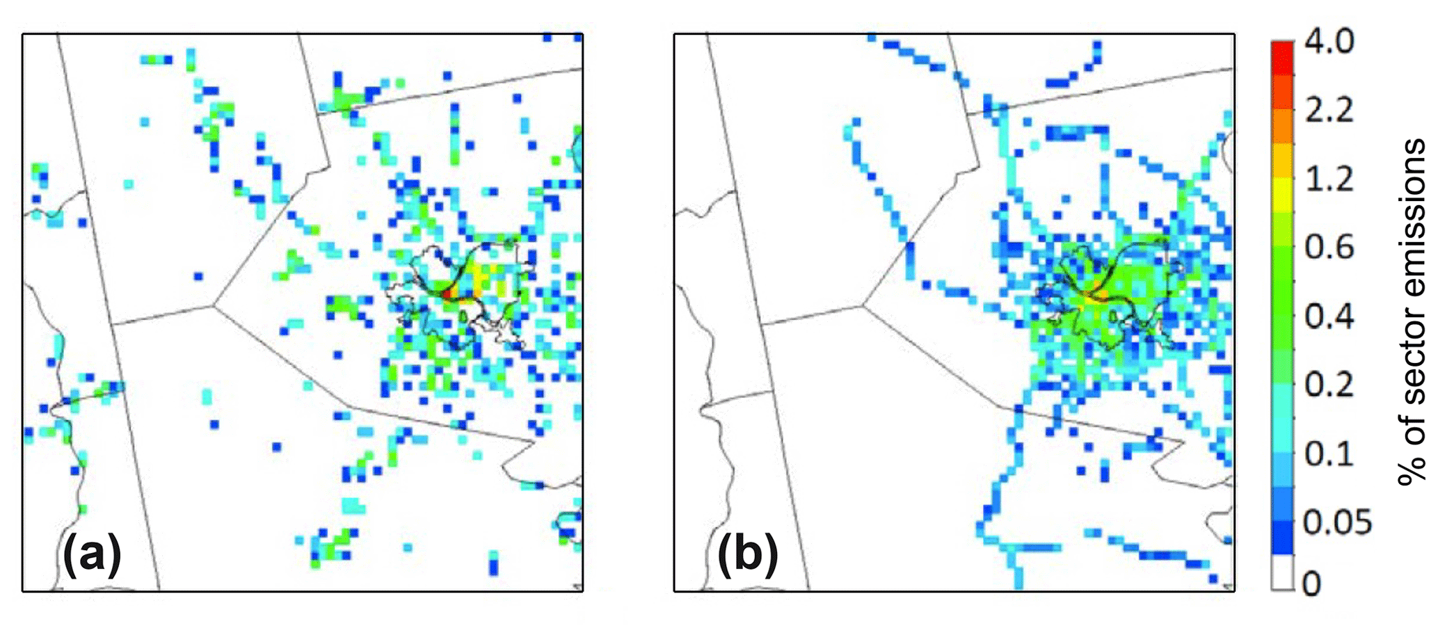
Figure 2Percentage of sector PM2.5 emissions in each 1×1 km computational cell for (a) commercial cooking and (b) on-road traffic in February 2017. The value of the colored points in each map add up to unity, corresponding to 100 % of emissions for the respective sector.
To accurately capture spatial patterns of on-road traffic, we use the output of a link-level, origin–destination by vehicle class traffic model of Pittsburgh (Ma et al., 2020). This traffic model simulates traffic counts and speed by hour of day using observations from Pennsylvania Department of Transportation sites throughout Pittsburgh. As expected, emissions in areas with major highways are high (Fig. 2b).
The novel surrogates used for on-road traffic and cooking result in increases in emissions in some areas and particularly in downtown Pittsburgh and decreases in others. Total emissions inside the inner 1×1 km domain are the same using both the new and old surrogates. For commercial cooking, emissions calculated using the new surrogates are more concentrated in areas with high restaurant densities such as downtown Pittsburgh and the Oakland neighborhood (Figs. S1 and S2 in the Supplement). For on-road traffic, the emissions become higher at the locations of major highways and in the urban area of Pittsburgh when using the new surrogates (Figs. S3 and S4). Using the new spatial distribution of emissions predicted average PM2.5 increase by 1–2 µg m−3 at certain areas. A detailed evaluation of these predictions will be the topic of another publication.
4.1 Effect of grid resolution
The results of the simulations with the four resolutions for the winter period are shown in Figs. 3 and 4. For the area of interest, the simulations at 36×36 km resolve concentration fields at the county scale. The urban–rural gradient is resolved in the 12×12 km simulations. Increasing the resolution to 4×4 km, large stationary sources such as power plants and large industrial installations are resolved. Finally, the resolution increase to 1×1 km resolves the intra-urban variations in Pittsburgh and medium-sized industrial installations. Variable concentration limits are used in the species maps to remove background and highlight the effects of local sources (Figs. 3 and 4).
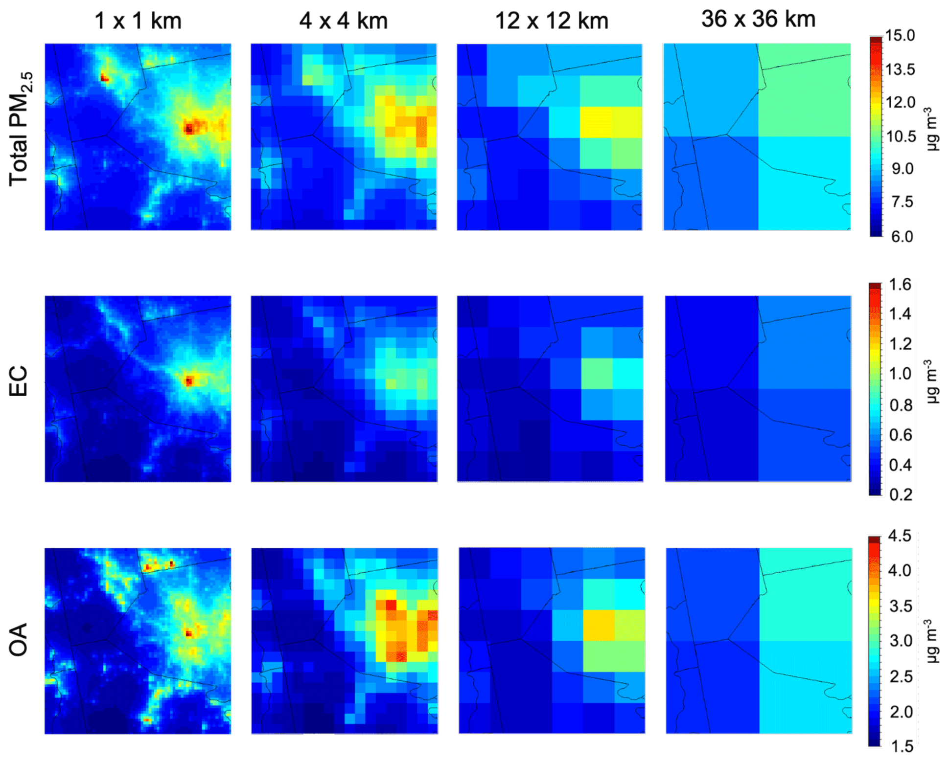
Figure 3Average predicted ground-level concentration of total PM2.5, EC, and OA at 36×36, 12×12, 4×4, and 1×1 km resolutions during February 2017. Different color scales that do not start from zero are used for the various maps.
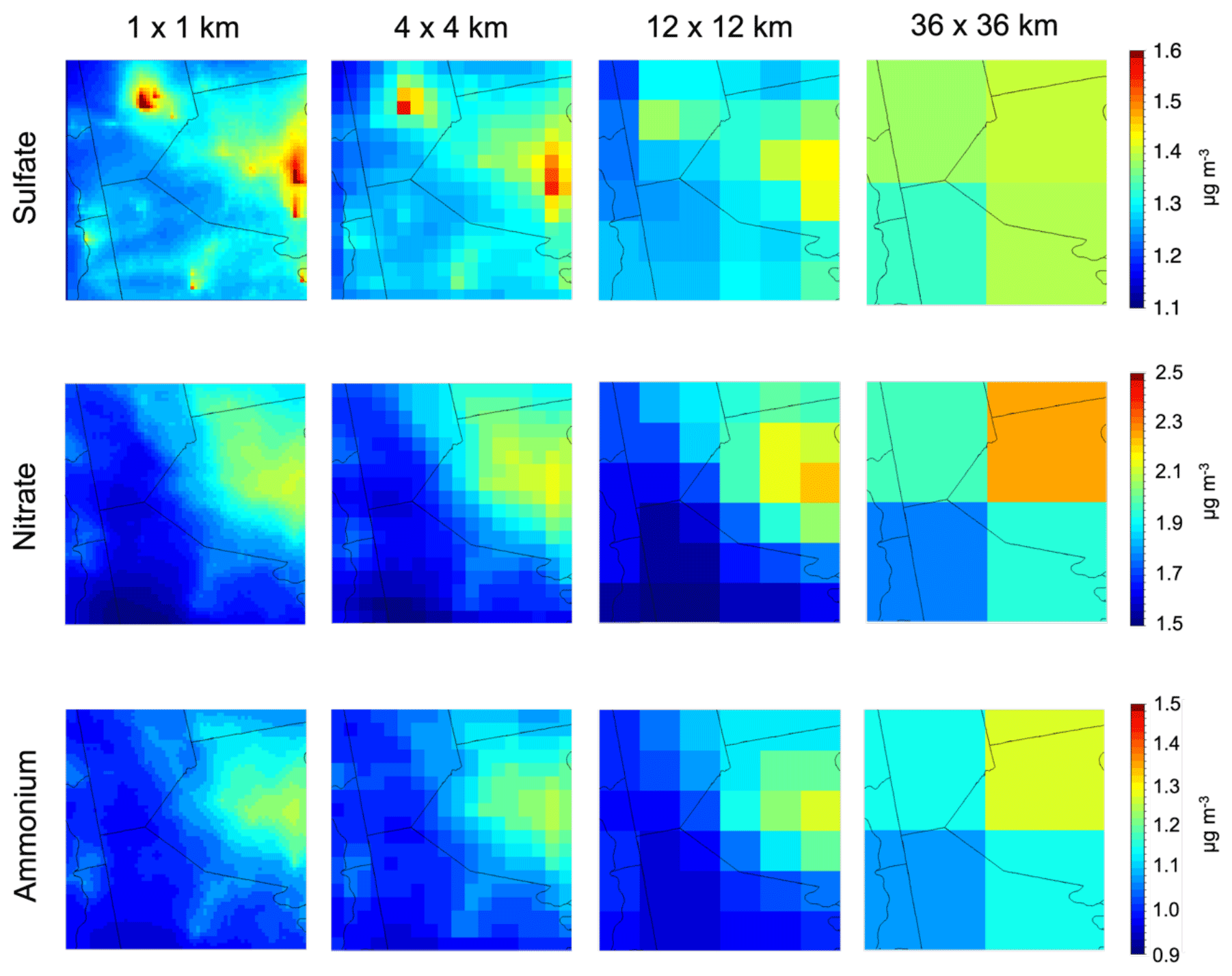
Figure 4Average predicted ground-level concentration of PM2.5 sulfate, nitrate, and ammonium at a 36×36, 12×12, 4×4, and 1×1 km resolution during February 2017. Different color scales that do not start from zero are used for the various maps.
In the winter period, the predicted maximum PM2.5 concentration in the inner domain increases from 10.4 µg m−3 at 36×36 km to 11.8 µg m−3 at 12×12, to 12.9 µg m−3 at 4×4, and finally to 16.4 µg m−3 at 1×1 km (Fig. 3), a 58 % increase. On the other end, the predicted minimum PM2.5 concentration changes from 8.2 µg m−3 at 36×36 km to 7 µg m−3 at 12×12 and remains practically the same at even higher resolutions. This corresponds to the background concentration level for the area during the simulation period, so further resolution enhancements do not change this value. The standard deviation of the predicted concentration can be used as a measure of the concentration variability in the area. This standard deviation changes from 0.9 µg m−3 at 36×36 to 1.24 µg m−3 at 12×12, to 1.45 µg m−3 at 4×4, and to 1.35 µg m−3 at 1×1 km. These results indicate an increase of the PM2.5 variability by 50 % when one moves from the coarse to the finest resolution. However, most of this change in variability (38 % out of the 50 %) appears when one moves from 36×36 to 12×12 km.
Elemental carbon is a primary aerosol component with sources that are quite variable in space. In winter, the predicted maximum PM2.5 EC increased by a factor of 2.9, from 0.6 µg m−3 at the 36×36 km resolution to 1.6 µg m−3 at 1×1 km (Fig. 3). The predicted maximum EC is located, as expected, in the Pittsburgh downtown area. On the other hand, the predicted minimum of EC is reduced by only 0.1 µg m−3, from 0.34 µg m−3 at 36×36 km to 0.24 µg m−3 at resolutions lower than or equal to 4×4 km. The standard deviation of the predicted EC almost doubles from 0.1 µg m−3 at 36×36 km to 0.18 µg m−3 at 1×1 km. Approximately 50 % of this increase in variability appears in the transition from the coarse to the intermediate resolution of 12×12 km. The fine and the finest resolutions are needed to resolve the other half of the predicted variability.
During this winter period a significant fraction (79 %) of the OA in the Pittsburgh area is primary, and therefore the higher resolution results in increases of the predicted maximum concentrations in space from 2.8 µg m−3 at the coarse resolution to 3.7 µg m−3 at the intermediate to 4.8 µg m−3 at the finest resolution (Fig. 3). This corresponds to an increase by a factor of 1.7, which is more than the change for total PM2.5 but much less than that for EC. The predicted maximum is located in downtown Pittsburgh, with additional hotspots in neighboring counties that are resolved at the fine and finest resolution. The predicted minimum changes from 2.1 µg m−3 at 36×36 to 1.7 µg m−3 at 12×12 with small reductions at higher resolutions. The variability (standard deviation) of the OA concentration field of the predicted concentration increases by a factor of approximately 1.6 from 0.35 µg m−3 at 36×36 to 0.51 µg m−3 at 12×12 km. The increase is small at even higher resolutions with the standard deviation of OA reaching 0.53 µg m−3 at 1×1 km (an increase by a factor of 1.7).
Average predicted PM2.5 sulfate in the inner domain changes little between the coarsest resolution (average level 1.37 µg m−3) and finest resolution (1.29 µg m−3). The minimum concentration decreased slightly with resolution from 1.33 to 1.2 µg m−3, with much of the decrease captured by increasing the resolution to 12×12 km. The maximum sulfate concentration increased by a larger value, but this change was not observed until moving to the highest resolution where the maximum was 2.08 µg m−3, compared to 1.4 µg m−3 at 36×36 km resolution. The standard deviation increased only marginally from 0.03 µg m−3 at 36×36 km to 0.06 µg m−3 at 1×1 km. The low variability in the predicted ground sulfate levels during the winter is partially due to the low mixing heights during this cold period with the emissions from the tall stacks of local power generation sources often introduced above the boundary layer.
The predicted fine nitrate levels are relatively high, ranging from 1.78 to 2.24 µg m−3 in the coarse-resolution simulation. This is expected in this wintertime period due to the partitioning of nitric acid and ammonium in the particulate phase. This predicted concentration range increases to 1.5–2.24 µg m−3 in the finest-scale simulation with higher levels in the northeast of the domain. The standard deviation of the predicted concentration does not show any significant trend changing from 0.19 µg m−3 at 36×36 to 0.15 µg m−3 at 1×1 km.
For PM2.5 ammonium, changes with increasing resolution are modest, with the predicted minimum being reduced from 1.07 µg m−3 at 36×36 to approximately 0.95 µg m−3 at all other higher resolutions. The predicted maximum stays relatively constant between 1.25 and 1.27 µg m−3 at all resolutions. As with nitrate, the standard deviation does not show any significant trend changing from 0.08 µg m−3 at 36×36 to 0.09 µg m−3 at 12×12 to 0.07 µg m−3 at 4×4 and 1×1 km resolutions.
4.2 Source apportionment
We performed zero-out simulations in the 1×1 km Pittsburgh grid to determine the local contributions of eight source categories to the total PM2.5. The local sources quantified included commercial cooking, industrial, biomass burning, on-road traffic, power generation, and miscellaneous area sources (Fig. 5). A summary of total local (within the inner 1×1 km resolution domain) dry PM2.5 emissions from each source category during February 2017 is shown in Table 1. The species category labeled “other” for the power generation sector is predominately composed of ash (including metals emitted from power generation) and is simulated in PMCAMx as inert particle mass. Biomass burning emissions here correspond only to residential wood combustion, as there were no significant wildfires in the 1×1 km resolution domain during the simulation periods. The PM2.5 emissions used in this study contain both the condensable and filterable fractions of PM2.5 (U.S. EPA, 2015). The miscellaneous area sources sector includes a large variety of emission sources that are not classified in any of the sources in Table 1. These include chemical manufacturing, solvent utilization for surface coatings, degreasing and dry cleaning, storage and transport of petroleum products, waste disposal and incineration, and cremation. The emissions from agricultural dust, river barges, off-road equipment, oil–gas activities, and rail were grouped in the “others” source. All emissions (particulate and gas phase) from each source were set to zero, and the results of the zero-out simulation were subtracted from those of the baseline simulation to estimate the corresponding source contribution. The contribution of long-range transport from outside the inner domain was also estimated by setting all local sources to zero.
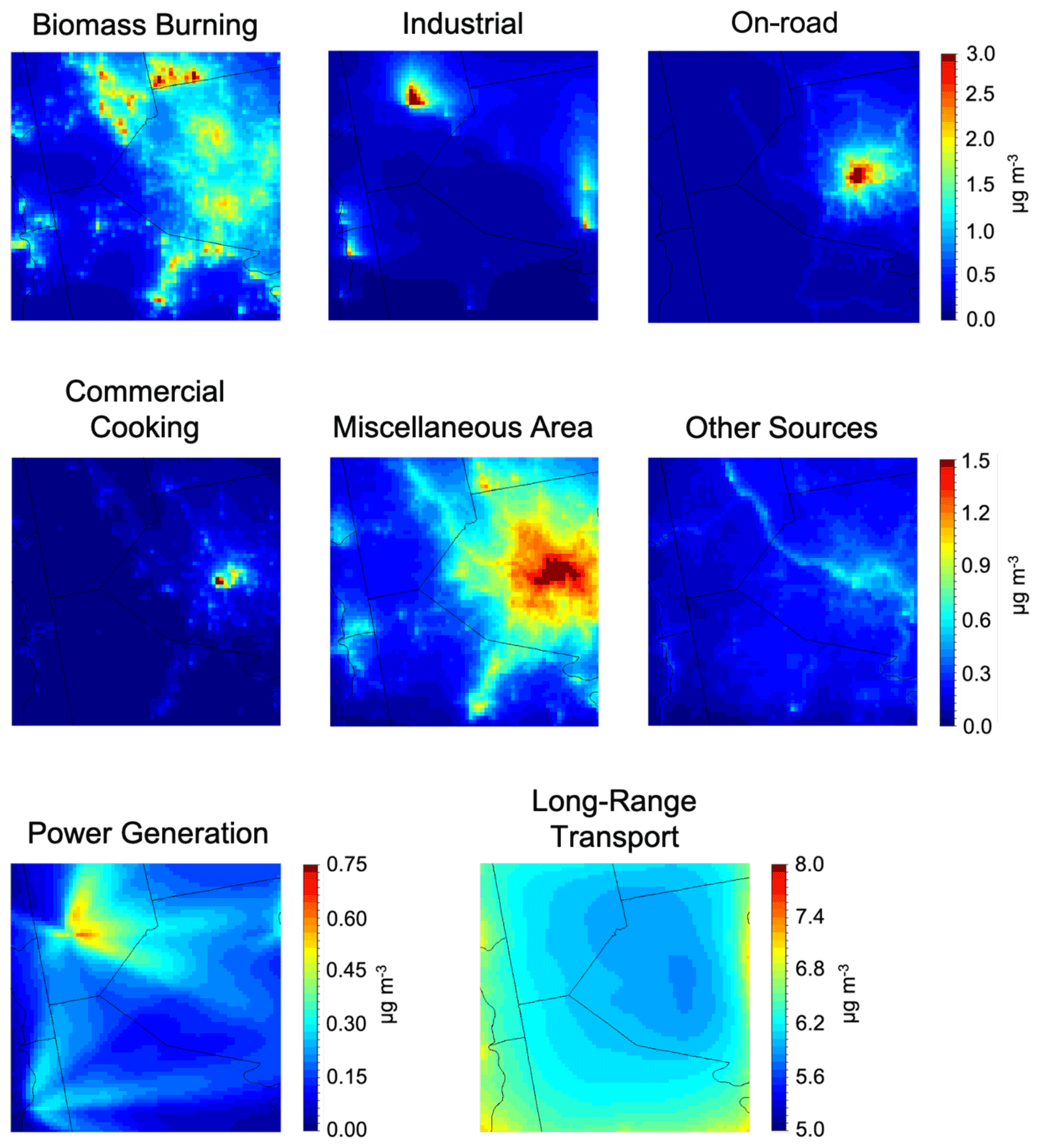
Figure 5Contribution of each source to total PM2.5 during February 2017. Different scales are used for the various maps.
Biomass burning is used during the winter for residential heating and recreation. This source contributes a maximum of 3.31 µg m−3 in Cranberry, a northern suburb of Pittsburgh located in the neighboring Butler County. In the downtown Pittsburgh area, the contribution from biomass burning accounts for 7 % of the PM2.5. This source shows the highest variability with a standard deviation of 0.5 µg m−3.
The maximum contribution of 8.05 µg m−3 from industry is predicted near a cluster of industrial facilities in the town of Beaver, 37 km northwest of Pittsburgh. The maximum PM2.5 concentration of the modeling domain is located here. In this location long-range transport contributes 37 % of the PM2.5 followed by industrial sources with 49 % and biomass burning with 7 %. On average, the contribution from industrial sources is low with 3.7 %. In downtown Pittsburgh, the contribution is lower still with 2 %.
On-road traffic emissions are most important in major highway intersections and river crossings surrounding downtown Pittsburgh with a maximum contribution of 3.9 µg m−3 accounting for 24 % of the PM2.5 in this area. On average, on-road traffic contributes 2.5 % of the PM2.5 mass. The contribution from on-road traffic shows higher variability (standard deviation: 0.36 µg m−3) since this sector contributes significantly to areas adjacent to the network of highways that radiates from the Pittsburgh downtown area.
On average, commercial cooking emissions contribute 0.7 % of the PM2.5 in the modeling domain with a maximum contribution of 2.44 µg m−3 in downtown Pittsburgh, with smaller contributions in the surrounding urban area. Cooking is predicted to account for 16 % of the PM2.5 mass in downtown Pittsburgh. The contribution from commercial cooking is localized around downtown Pittsburgh and therefore shows little variability throughout the domain with a standard deviation of 0.1 µg m−3.
The miscellaneous area source sector contributes 6 % of the PM2.5 on average. Since this sector encompasses a variety of sources and activities, its contribution shows significant variability with a standard deviation of 0.34 µg m−3. The maximum contribution is located in the Pittsburgh urban core with 1.64 µg m−3, accounting for 11 % of the PM2.5.
The power generation sector contributes a maximum of 0.63 µg m−3 in the plume of the Bruce Mansfield Power Plant northwest of Pittsburgh (this plant is no longer operating as of 2019). The contribution of this sector shows the smallest variability at 0.09 µg m−3. The contribution to ground PM2.5 from power generation in the winter is relatively low. This is largely due to the height of the emissions stacks associated with this sector. A significant fraction of the emissions from power generation is trapped above the shallow mixing height in the winter, and much of the PM2.5 mass is predicted to remain in the upper air layers. The predicted relative high upper air PM2.5 concentration from power generation is shown in Fig. S5.
Long-range transport from outside the inner modeling domain is the major source of PM2.5 during this period, contributing an average of 74 %. This contribution varies from 7.1 µg m−3 in the southeast corner of the domain and decreases in the direction of the Pittsburgh urban core where the contribution is reduced to 5.9 µg m−3. In areas where there are significant local emissions such as the Pittsburgh downtown area, the contribution from long-range transport decreases to 38 %.
Contributions for all remaining sources are largest in the Pittsburgh downtown area with 0.74 µg m−3, accounting for 5 % of the PM2.5. This sector also significantly contributes on the Ohio and Monongahela River valleys, where there is important rail and river traffic. On average, these sources contribute 3 % of the PM2.5 and show a moderate variability with a standard deviation of 0.1 µg m−3.
For all local sources, the minimum contribution is close to zero (less than 0.1 µg m−3) and is located at the southwestern corner of the domain, near the Ohio–West Virginia border.
5.1 Effect of grid resolution
The predicted PM2.5 concentrations in the simulated summer period are lower than during the winter period and more uniform; however, the qualitative behavior of the model at the different scales remains the same (Fig. 6). Variable concentration limits are again used in these maps to remove background and highlight the effects of local sources. The standard deviation of the PM2.5 increases from 0.28 µg m−3 at 36×36 to 0.57 µg m−3 at 12×12, to 0.72 µg m−3 at 4×4, and to 0.82 µg m−3 at 1×1 km. At the finest scale, the predicted variability in the summer is 61 % of that in the winter. Similar to the winter period, the predicted maximum PM2.5 concentration changes significantly with increasing resolution. The predicted maximum PM2.5 increases from 6.4 µg m−3 at the coarse to 15.3 µg m−3 at the fine resolution. The finest scale better resolves the concentration field in the cluster of industrial installations 37 km northwest of Pittsburgh. The minimum PM2.5 drops from 6.5 µg m−3 at 36×36 to 5.3 µg m−3 at 12×12 and then to 4.7 µg m−3 at 1×1 km. As in the winter period, the moderate resolution appears to capture the majority of the concentration change from increasing resolution (67 %).
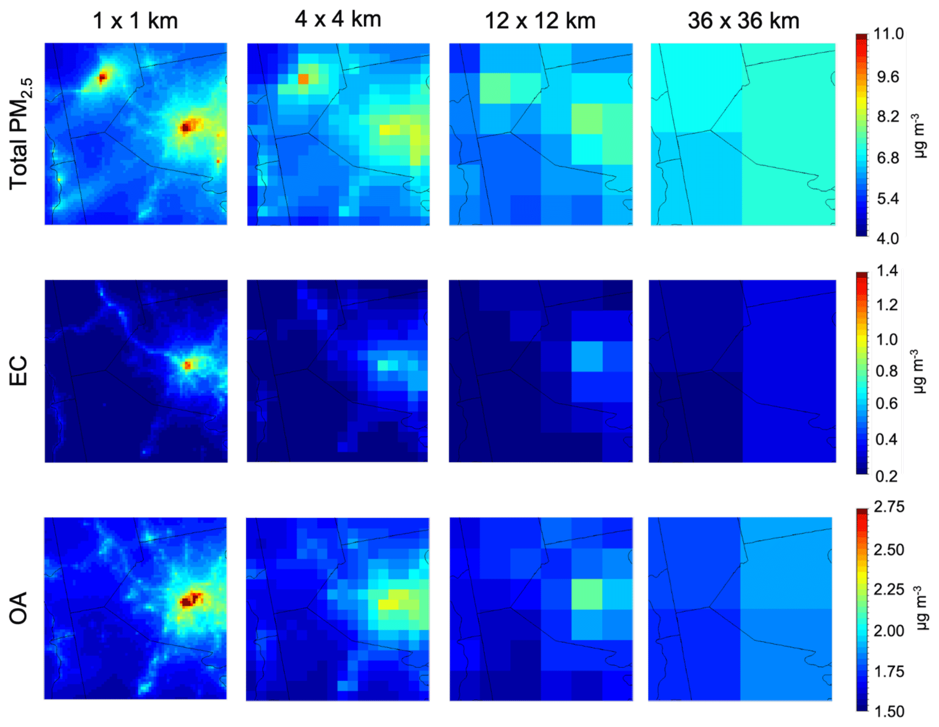
Figure 6Average predicted concentration at the ground level of total PM2.5, EC, and OA at a 36×36, 12×12, 4×4, and 1×1 km resolution during July 2017. Different color scales that do not start from zero are used for the various maps.
The average EC is lower during the summer with 0.28 µg m−3 versus 0.43 µg m−3 in the winter. The standard deviation of the predicted average EC increases from 0.06 µg m−3 at 36×36 to 0.09 µg m−3 at 12×12 to 0.11 µg m−3 at 4×4 km and to 0.13 µg m−3 at 1×1 km. The peak average EC is located in downtown Pittsburgh and increases by a factor of 3.6 (from 0.35 to 1.27 µg m−3) moving from the coarse to the finest resolution. It is noteworthy that the peak is 38 % less than that of the winter when the coarse resolution is used but only 21 % when the finest resolution is used. The concentration range (difference between the maximum and the minimum) increases from 0.13 to 1.12 µg m−3 moving from the coarse to the finest resolution. This increase by a factor of 8.6 shows the importance of the local variations of a primary species like EC in an urban area in both summer and winter.
The OA concentration field is quite uniform at the coarse scale varying by only 0.17 µg m−3 (from 1.72 to 1.89 µg m−3) with a standard deviation of 0.07 µg m−3 (Fig. 6). Variability increases significantly when one moves to the finest scale, with the range increasing to 2.24 µg m−3 (from 1.55 to 3.79 µg m−3), and the standard deviation of the OA field increases to 0.2 µg m−3. The use of the finest scale appears to be needed for the resolution of the OA high-concentration areas in the summer more than in the winter.
The PM2.5 sulfate levels during the summer period are on average 12 % higher that during the winter one. At the coarse and intermediate scales, the predicted average concentration fields have relatively little structure (Fig. 7). The corresponding concentration ranges are relatively narrow (0.05 µg m−3 at 36×36 km and 0.42 µg m−3 at 12×12 km). However, a different picture emerges at the fine and especially the finest scales. The plumes from the major power plants can be clearly seen at these higher resolutions. The maximum increased by 0.5 µg m−3 from the coarse scale to the finest scale, while the minimum is reduced from 1.78 µg m−3 at 36×36 to 1.05 µg m−3 at 12×12 to 0.95 µg m−3 at 4×4 and 1×1 km. The standard deviation of the predicted sulfate concentration field at the coarse resolution is low and similar to that in winter, 0.02 µg m−3. However, the variability at the finest scale in the summer (0.13 µg m−3 at 1×1 km) is twice the predicted variability in the winter.
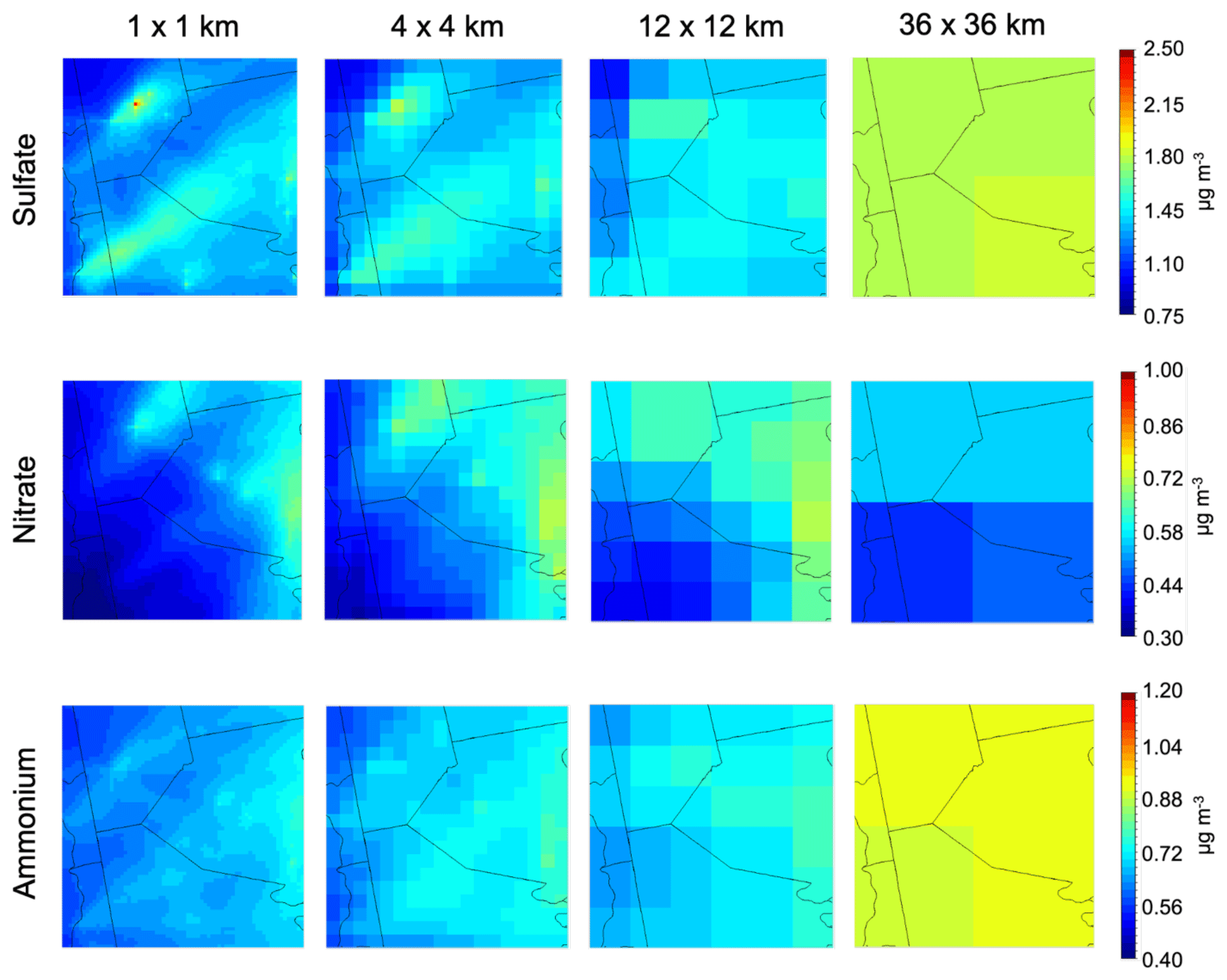
Figure 7Average predicted concentration of PM2.5 sulfate, nitrate, and ammonium at a 36×36, 12×12, 4×4, and 1×1 km during July 2017. Different color scales that do not start from zero are used for the various maps.
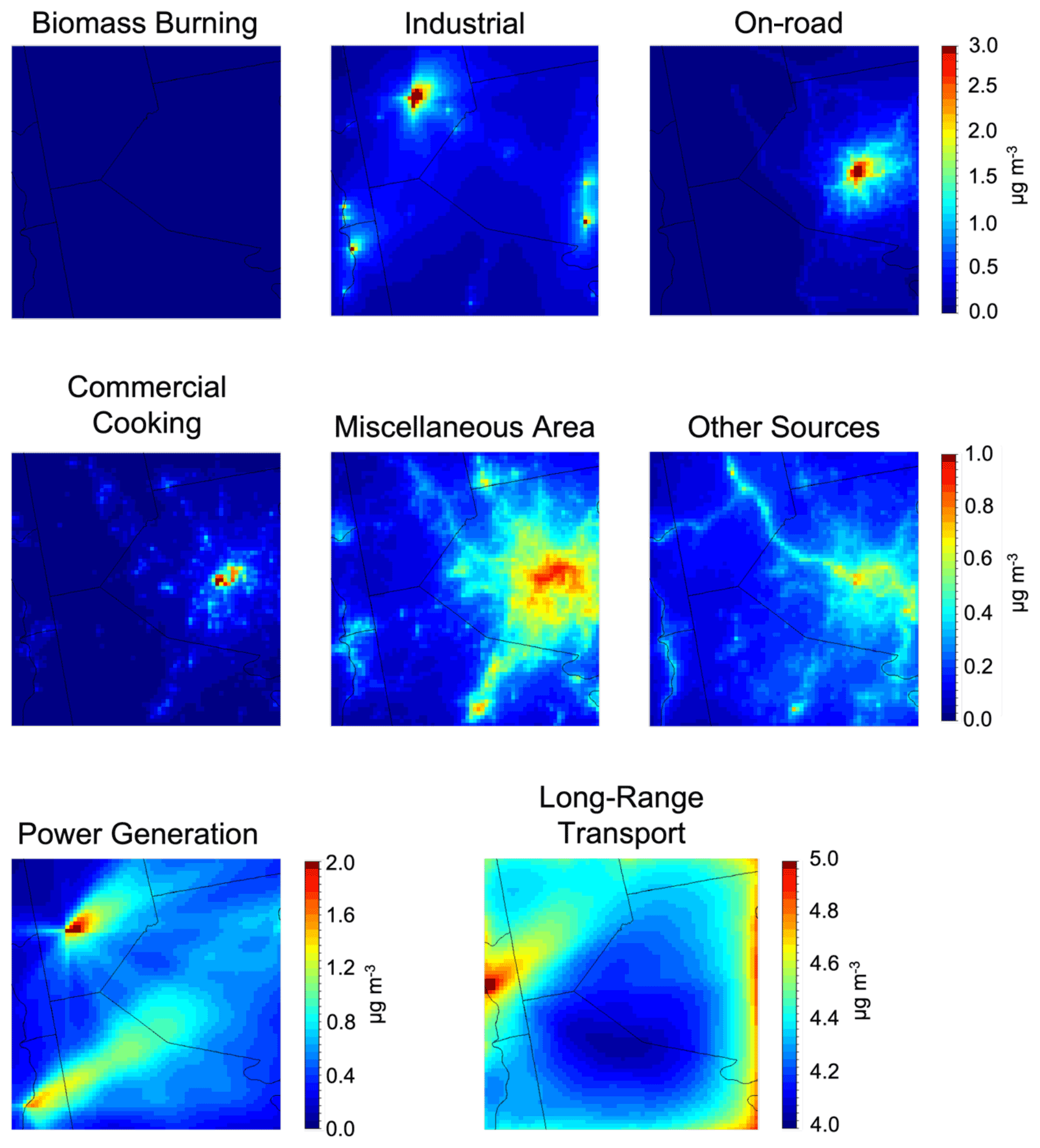
Figure 8Contribution of each source to total PM2.5 during July 2017. Different scales are used for the various maps.
The predicted summertime nitrate concentrations are quite low in the area (average 0.5 µg m−3 in the coarse and 0.46 µg m−3 in the finest resolution). The predicted minimum decreases from 0.42 µg m−3 at 36×36 to 0.39 µg m−3 at 12×12, to 0.34 µg m−3 at 4×4, and to 0.3 µg m−3 at 1×1 km. The predicted maximum concentration increases from 0.56 µg m−3 at the coarse scale to 0.71 µg m−3 at the intermediate scale and stays relatively constant at higher resolutions. The concentration field is quite uniform, with a standard deviation ranging from 0.06 to 0.09 µg m−3 for all scales. However, due to the reduction in the predicted minimum the concentration range increases from 0.14 µg m−3 at the coarse resolution to 0.37 µg m−3 at the finest resolution.
The PM2.5 ammonium concentration field is quite uniform at all resolutions (Fig. 7). The concentration range increases from 0.04 to 0.22 µg m−3 moving from the coarse to the finest resolution, and the standard deviation increases from 0.02 to 0.04 µg m−3.
5.2 Source apportionment
The local emissions for each source category during July 2017 are shown in Table 2. During summer, residential biomass burning is minimal (Fig. 8). This source contributes a maximum of 0.04 µg m−3 and an average of 0.007 µg m−3, accounting for 0.6 % of the average total PM2.5.
Power generation sources have the highest average contribution to total PM2.5 of all the local sources of 10 %. Industrial sources account for 6 % of the average PM2.5 but are the most important contributor in the point of the modeling domain with the maximum predicted PM2.5 concentration. At this location in Beaver County, industrial sources account for 58 % of total PM2.5
As in the winter period, on-road traffic emissions have the largest contribution to the PM2.5 in the downtown Pittsburgh area where four large highways intersect. In this location on-road traffic contributes 26 % of the PM2.5. On average, local on-road traffic contributes around 3 % of the PM2.5 mass. During the summer period, the variability of the on-road traffic contribution is slightly lower with 0.33 µg m−3 compared with 0.36 µg m−3 during winter.
Commercial cooking emissions contribute a maximum of 2.08 µg m−3 to the average total PM2.5 in downtown Pittsburgh. This source accounts for 17 % of the PM2.5 in the city but only 1 % for the entire modeling domain. The large predicted contribution from cooking PM2.5 is consistent with the mobile AMS measurements performed by Ye et al. (2018), which indicated that cooking organic aerosol contributes up to 60 % of the non-refractory PM1 mass. Mobile AMS results from Gu et al. (2018) showed that cooking OA contributes 5 %–20 % of PM1 mass over multiple areas in the city of Pittsburgh. Other measurements in Pittsburgh also showed that cooking OA concentrations were clearly elevated in the vicinity of restaurants when compared with residential areas (Robinson et al., 2018). Though the cooking PM2.5 mass predictions of our study cannot be directly compared to these measurements, they all highlight the local importance of cooking as a fine-PM pollution source.
On average, the miscellaneous area sources sector contributes 0.26 µg m−3, accounting for 4.3 % of the PM2.5. In downtown Pittsburgh, where the contribution is highest, this source contributes 7 % of the PM2.5.
Unlike in the winter period, the plumes from major powerplants in the Ohio River valley are clearly resolved in the summer. The power generation sector contributes a maximum of 2.4 µg m−3 in the plume of the Bruce Mansfield Power Plant northwest of Pittsburgh. On average, the 9.4 % contribution from this sector to the PM2.5 is much larger than in the winter where it only contributed 2.3 %. The plume from the Mitchell Power Plant in the southwest corner of the modeling domain is clearly resolved and reaches all the way to the city. This increases the contribution from power generation to the PM2.5 in the downtown core from 0.22 µg m−3 in the winter to 0.61 µg m−3 in the summer. The maximum contribution of 8.98 µg m−3 from industrial sources is a cluster of industrial facilities in the town of Beaver, northwest of Pittsburgh.
Long-range transport from sources outside the region contributes a maximum of 5.2 µg m−3 in the southeast corner of the domain, decreasing in the direction of the Pittsburgh northern suburbs where the contribution is minimal with 4.1 µg m−3. On average, long-range transport accounts for 72 % of the PM2.5 mass. In downtown Pittsburgh, long-range transport contributes 4.24 µg m−3, accounting for 35 % of the PM2.5. The high-concentration area visible on the western edge of the domain is due to a cluster of power generation and industrial sources located in the Ohio River valley just outside of the inner modeling domain.
On average, the contribution from all remaining sources is 3.6 % and shows a moderate variability of 0.1 µg m−3. The contribution from these sources is maximal in downtown Pittsburgh, with 0.78 µg m−3 accounting for 6 % of the PM2.5.
For all local sources, the minimum contribution is close to zero (less than 0.1 µg m−3) and is located at the northwestern corner of the domain, near the Ohio–Pennsylvania border.
Relative contributions of all local sources to domain average predicted total PM2.5 (including long-range transport PM2.5 mass) are shown in Fig. 9. The largest differences between February and July are the contributions from biomass burning and power generation. In the winter, biomass burning is the most important local source of PM2.5, contributing over 8 %. In the summer, this source contributes much less than 1 % to total PM2.5. This discrepancy can easily be explained by the lack of residential wood combustion in the warmer months of the year. Power generation is a significantly more important source in July than in February. This is likely a result of a lower mixing height in the winter combined with emissions plumes from power plants in the Ohio River valley originating from very tall stacks.
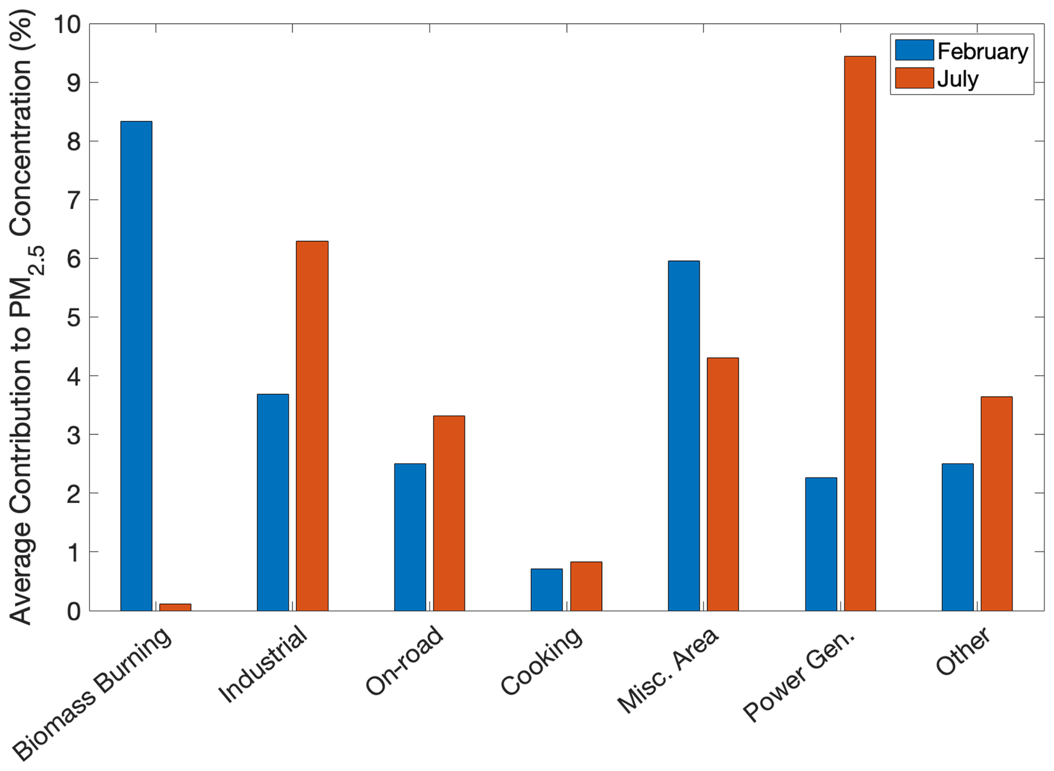
Figure 9Relative contributions of local sources to average predicted total PM2.5 concentrations in the inner 1×1 km resolution domain during February and July 2017.
The relative contributions of local sources to average predicted total PM2.5 in the maximum concentration cell in Beaver County and in downtown Pittsburgh are shown in Figs. 10 and 11, respectively. The dominant local source in the Beaver County location is industrial emissions, due to the proximity of various industrial installations in this area. Industrial sources here account for around 49 % of total PM2.5 in February and 58 % of total PM2.5 in July. A lot of the difference in industrial PM2.5 at the Beaver County location between months is made up by biomass burning in February, which accounts for 7 % more of the total compared to July. In the downtown area of Pittsburgh, the majority of PM2.5 from local sources can be attributed to either traffic (22 %–27 % of total PM2.5) or cooking (16 %–18 % of total PM2.5) in both simulation periods (Fig. 11).
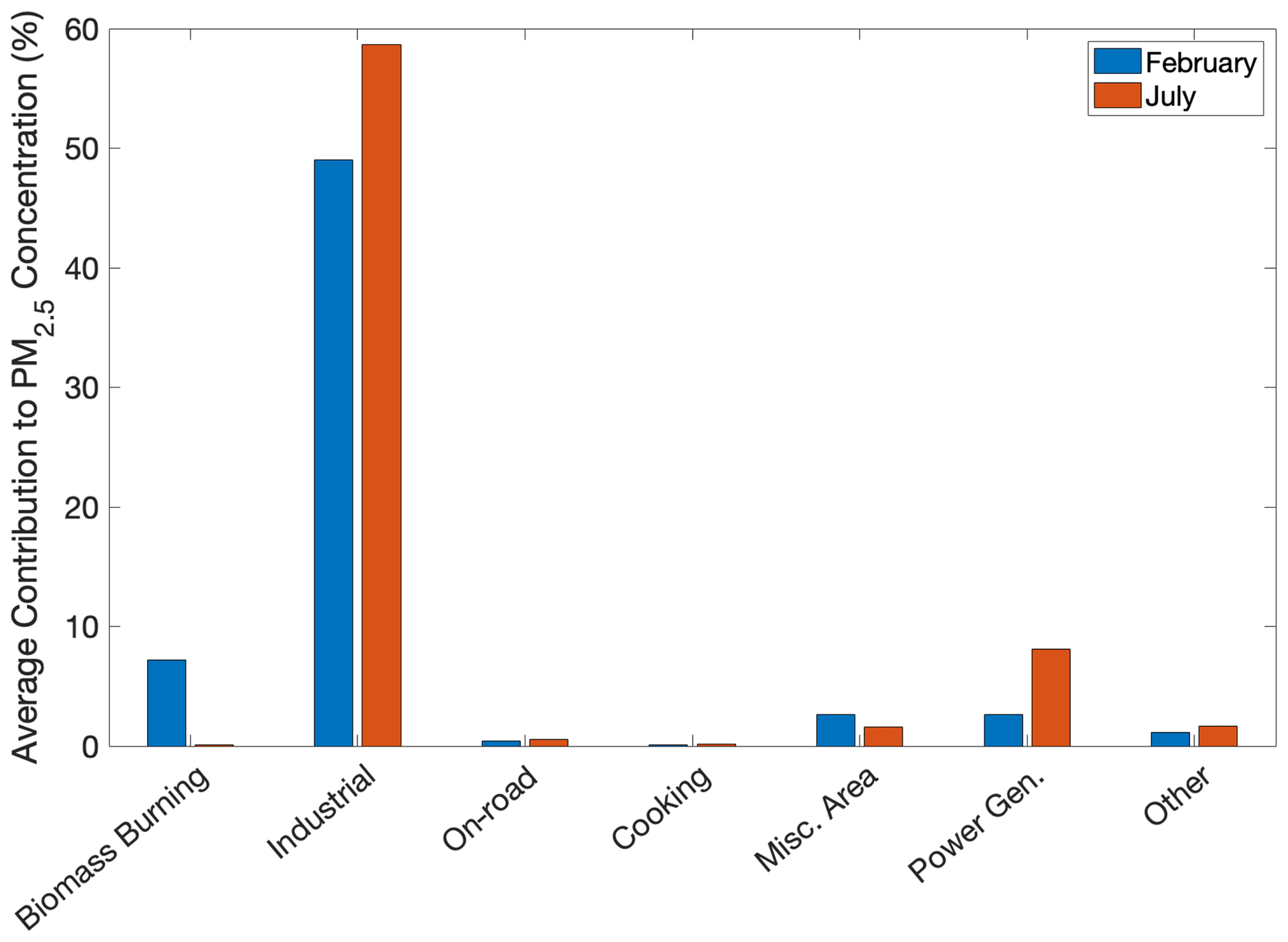
Figure 10Relative contributions of local sources to average predicted PM2.5 concentrations at the location of highest average concentration (Beaver County) during February and July 2017.
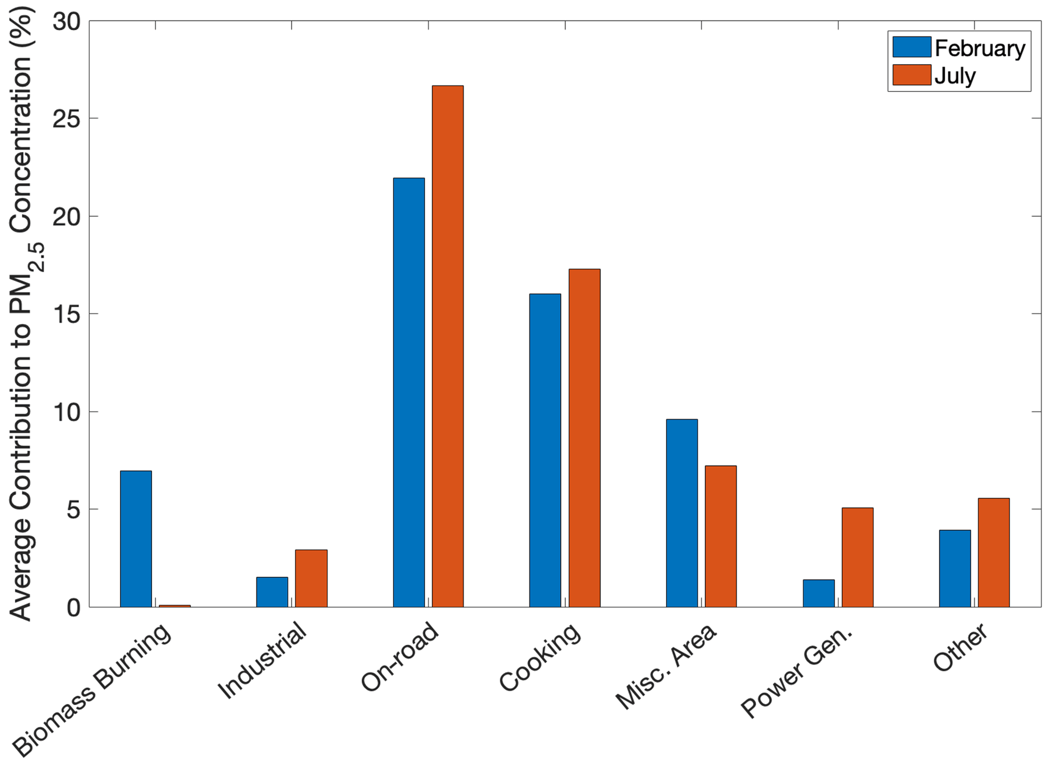
Figure 11Relative contributions of local sources to average predicted total PM2.5 concentrations in downtown Pittsburgh during February and July 2017.
The population data in the inner domain from the 2010 US census were used to estimate the exposure of the population in the Pittsburgh area to model predictions of PM2.5 during winter of 2017 at the different grid resolutions. We ranked the average PM2.5 concentrations from all the cells in the modeling domain and created bins of 0.2 µg m−3. A sum of the population from all the grid cells that fall within each concentration bin was calculated and divided by the total population of the inner grid to construct population exposure histograms. The population data used here is resolved at the census group level, which is much smaller than the simulation grid cell size of 1×1 km.
6.1 Winter PM2.5 exposure
Figure 12 shows the population exposure histograms for the Pittsburgh area (inner domain) for each model resolution. At the coarse resolution, there are only four PM2.5 values and 46 % of the population is exposed to a concentration of 10.4 µg m−3 with decreasing exposure with PM2.5 concentration. At a 12 km resolution, the low-concentration side of the distribution is better resolved, but gaps can still be observed at higher levels. At this intermediate resolution, the largest fraction of the population (15 %) is exposed to PM2.5 concentrations of 11.8 µg m−3.
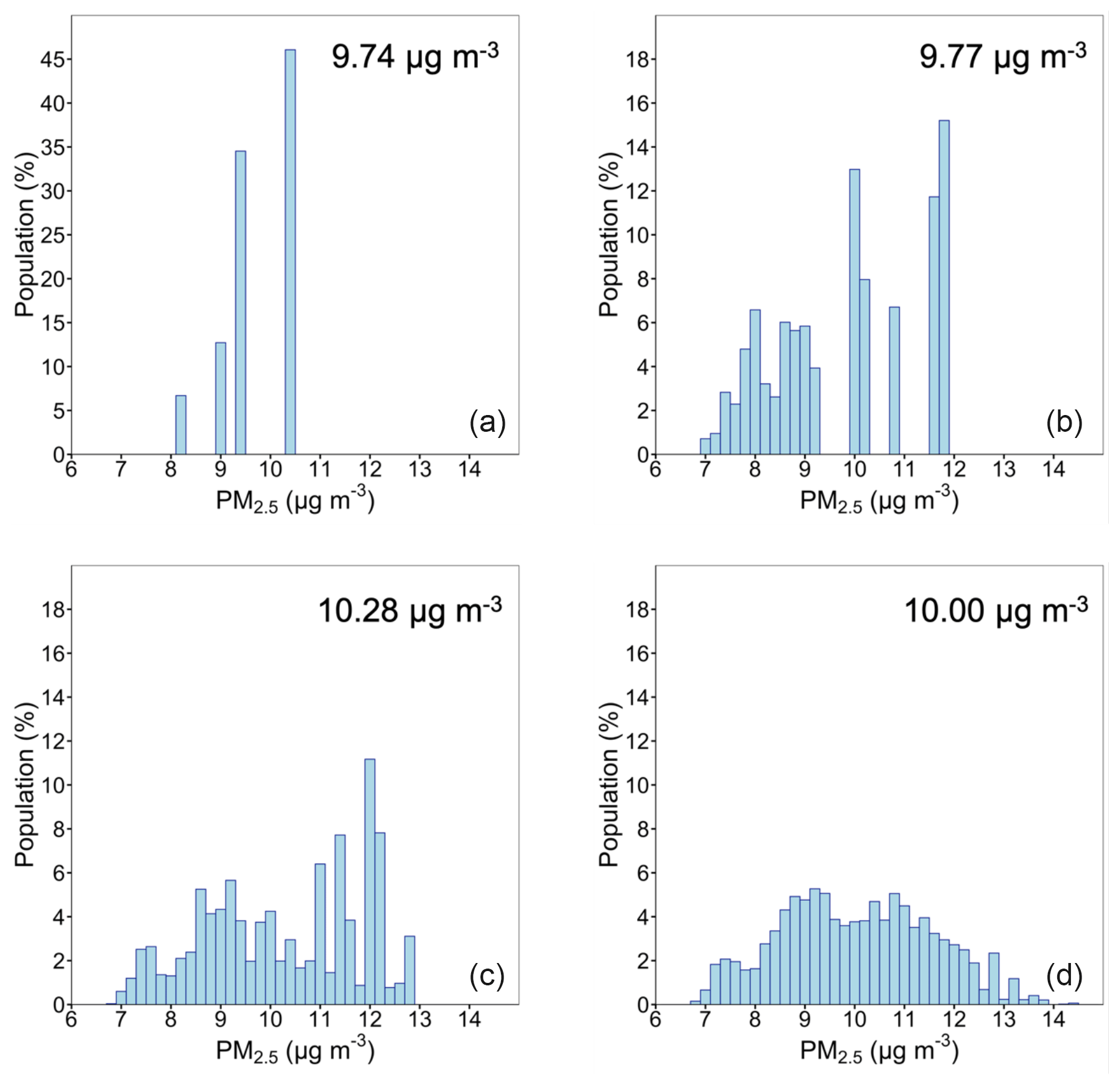
Figure 12Population exposure histograms at (a) 36×36, (b) 12×12, (c) 4×4, and (d) 1×1 km during February 2017. A different scale for population is used for the distribution at 36×36 km resolution. The average population-weighted PM2.5 concentration for each resolution is shown in the upper right corner of each window.
When the resolution is increased to 4 km the biggest improvements on the model ability to resolve the exposure distribution happen at concentrations higher than 9.4 µg m−3. At the fine resolution, no gaps appear in the distribution. A maximum of 12 % of the population is exposed to PM2.5 concentrations of 12 µg m−3, while at the highest concentration of 12.8 µg m−3, 3 % of the population is exposed. At the 1 km resolution, the distribution is much smoother due to the ability of this finest grid to capture local gradients. The largest fraction of the population (6 %) is exposed to PM2.5 concentrations of 9.2 µg m−3. At the highest concentration of 14.4 µg m−3 the exposed population is less than 0.1 % as this maximum point is located near industrial installations 37 km northwest of Pittsburgh where the population density is very low.
The differences between the predicted exposure distributions at 4 and 1 km resolutions highlight the need for high-resolution modeling studies in order to identify key areas from the environmental justice perspective. The upper tail of the exposure distribution (13–14 µg m−3) is only detectable at the 1 km resolution. These higher exposures could be addressed by appropriate targeted regulations, because they are the direct result of proximity to either major industrial and electrical generation sources or dense traffic and cooking emissions.
At resolutions of 36, 12, 4, and 1 km the predicted average population-weighted total PM2.5 concentration during February 2017 is 9.74, 9.77, 10.28, and 10.00 µg m−3, respectively. This represents an increase of only 2.6 % when moving from lowest to highest resolution. Relative contributions of local sources to average population-weighted PM2.5 concentration are shown in Fig. 14. Compared to the domain average PM2.5 concentrations (Fig. 9), many local source contributions are enhanced in terms of average population exposure. In February, weighting PM2.5 concentrations by population increases the contribution from biomass burning from 8.3 % to 11.7 %. Other notable increases include on-road traffic (2.5 % to 6.5 %) and miscellaneous area sources (5.9 % to 9.2 %). Other local source contributions to population-weighted PM2.5 were similar to the corresponding non-weighted concentrations.
The source-resolved population exposure distributions during this winter period are shown in Figs. S6 and S7.
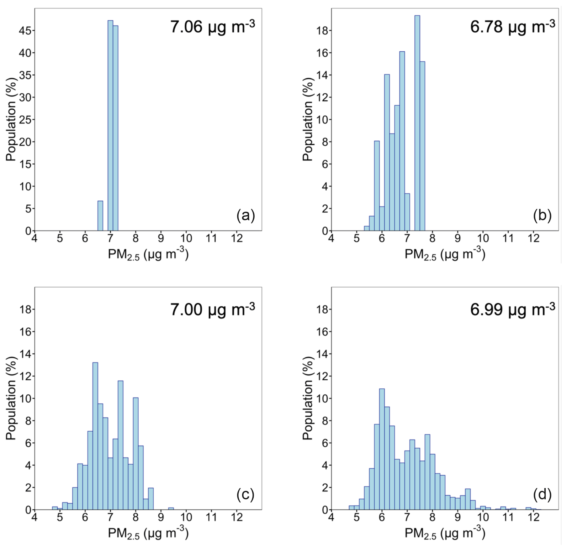
Figure 13Population exposure histograms at (a) 36×36, (b) 12×12, (c) 4×4, and (d) 1×1 km during July 2017. A different scale for population is used for the distribution at 36×36 km resolution. The average population-weighted PM2.5 concentration for each resolution is shown in the upper right corner of each window.
6.2 Summer PM2.5 exposure
Figure 13 shows the population exposure for each simulation grid during the summer period. At the coarse resolution, 88 % of the population is exposed to a concentration of 7 to 7.2 µg m−3. At 12×12 km resolution, the exposure distribution is better resolved, but a gap is still present at 7.2 µg m−3, and exposure to PM2.5 concentrations above 7.6 µg m−3 is not resolved at all. At this intermediate resolution, the largest fraction of the population (19 %) is exposed to PM2.5 concentrations of 7.4 µg m−3. Increasing the resolution to 4×4 km both shifts the distribution to slightly lower concentrations and resolves exposure to higher PM2.5 concentrations than with the 12×12 km grid. At this resolution, 14 % of the population is exposed to 6.4 µg m−3, and smaller portions of the population are exposed to concentrations higher than 8.0 µg m−3. Moving to the highest resolution grid further resolves the exposure distribution. Most notably, 1×1 km resolution reveals a bimodal distribution of population exposure, with one peak centered around 6.0 µg m−3 and another centered around 7.4 µg m−3. This likely corresponds to one subset of the population in the urban areas of Pittsburgh which are exposed to higher PM2.5 concentrations and another subset representing the surrounding suburban areas.
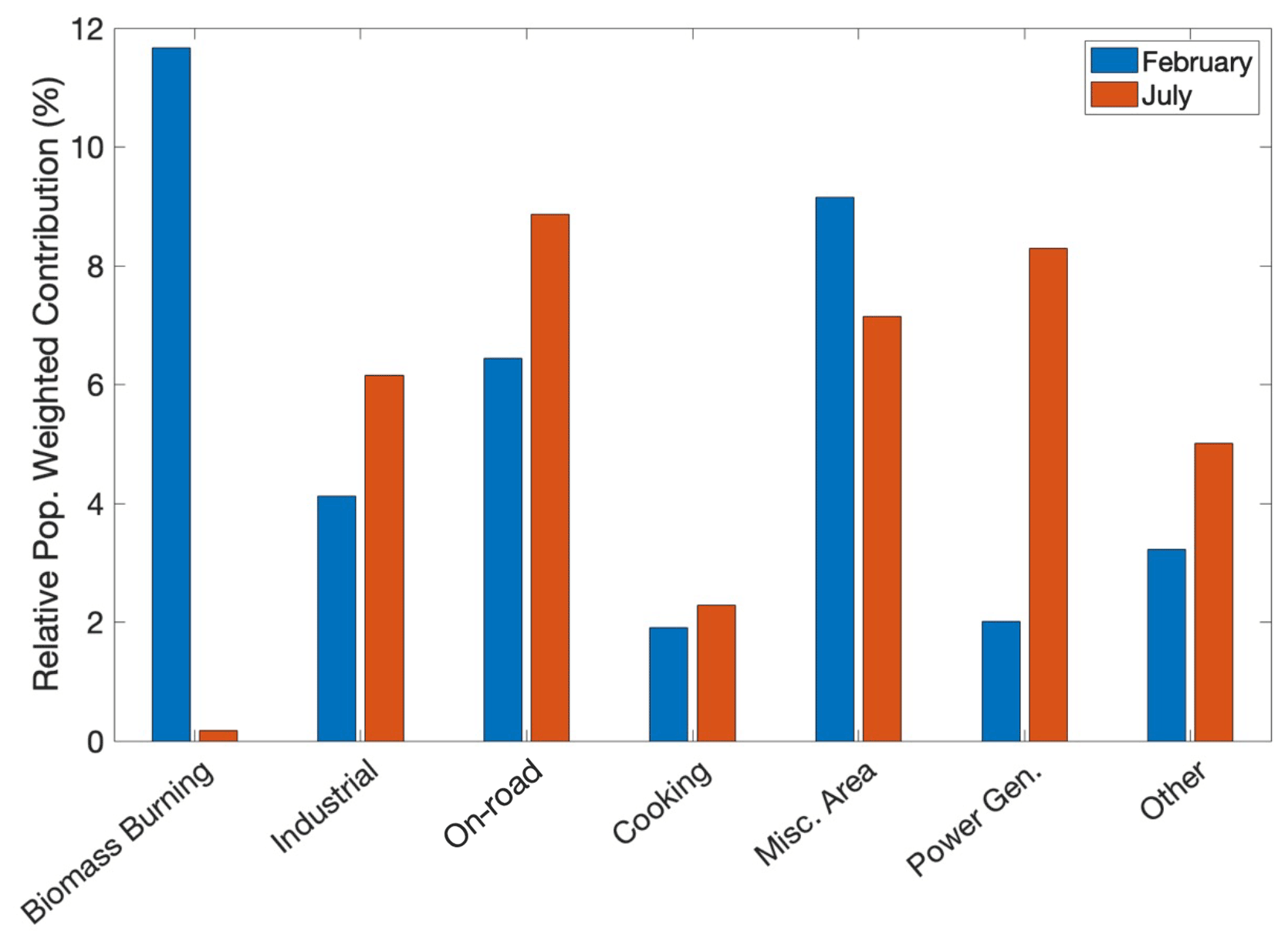
Figure 14Relative contributions from local sources to population-weighted total PM2.5 concentration for February and July 2017.
In the summer period, an even larger range of high-concentration exposure is revealed moving from 4 to 1 km resolution. At this high resolution, the population exposure to concentrations ranging from 8.5 to 12 µg m−3 becomes clear. Most people exposed to these higher fine-PM levels according to PMCAMx live in the vicinity of the industrial complexes and power stations around the city of Beaver. The higher concentration range of the upper tail of the exposure during July compared to February is due to a large extent to the effective mixing of the emissions from the tall stacks down to the ground level.
At resolutions of 36, 12, 4, and 1 km the predicted average population-weighted total PM2.5 concentration during February 2017 is 7.06, 6.78, 7.0, and 6.99 µg m−3, respectively. This represents just a 1 % decrease between the lowest and highest resolutions. Similar to the effect seen in February, weighting PM2.5 concentrations by population increases the contribution from on-road traffic from 3.3 % to 8.9 % in July. Contributions from miscellaneous area sources also increased (4.3 % to 7.1 %) when weighting by population. The population-weighted contribution from power generation sources in July decreased from the non-weighted value from 9.4 % to 8.3 %. All other local source contributions to population-weighted PM2.5 in July were similar to the non-weighted values.
The source-resolved population exposure distributions during this summer period are shown in Figs. S8 and S9.
We applied the PMCAMx chemical transport model over the city of Pittsburgh for the simulation periods of February and July 2017 using a series of telescoping grids at 36×36, 12×12, 4×4, and 1×1 km. Emissions were calculated using 2017 projections from the 2011 NEI. Emissions were distributed geographically using the spatial surrogates provided with the NEI11 for all grids. For commercial cooking, a new 1×1 km spatial surrogate was developed using restaurant count data from the Google Places API. Traffic model data were used to develop a 1×1 km spatial surrogate for on-road traffic emissions.
At the coarse resolution, county-level differences can be observed. Increasing the resolution to 12×12 km resolves the urban–rural gradient, and further increasing to 4×4 resolves large stationary sources such as power plants. Only at the finest resolution, intra-urban variations and individual roadways are resolved. Low-variability, regional pollutants such as nitrate show limited improvement after increasing the resolution to 12×12 km, while predominantly local pollutants such as elemental carbon and winter organic aerosol have gradients that can only be resolved at the finest resolution.
Biomass burning shows the largest variability during the winter period with many local maxima and significant emissions within the city and in the suburbs. During the summer contributions from this source are negligible. In contrast with the winter period, during the summer the plumes from large power plants in the Ohio River valley can be resolved. These plumes are rich in sulfates and start being resolved at 4×4 km, with significant detail added at 1×1 km. During both periods the largest contributing source to the average PM2.5 is particles from outside the modeling domain.
The ability of the model to resolve the exposure distribution increases at different rates according to the concentration. A significant improvement in resolving exposure to concentrations below 9.4 µg m−3 in the winter and below 7.0 µg m−3 in the summer is achieved by increasing the resolution to 12×12 km. Only at the finest resolution is the exposure to concentrations above 9.6 µg m−3 in the winter and above 8.6 µg m−3 in the summer fully resolved as well as the impact of high-concentration spots.
The average exposure in terms of average contribution to population-weighted PM2.5 concentrations of some local sources is enhanced compared to the non-weighted average PM2.5 concentrations. In February, weighting by population enhanced the contributions from biomass burning, on-road traffic, and miscellaneous area sources by 3 %–4 %. In July, the contributions from on-road traffic and miscellaneous area sources also increased by 3 %–5 % from this procedure.
It was determined that increasing simulation grid resolution from 36×36 to 1×1 km had minimal effect on the predicted domain average population-weighted PM2.5 concentration. Moving from the lowest to highest grid resolution increased the predicted average population-weighted PM2.5 by less than 3 %. In July, the average decreased by 1 %. This negligible change in the predicted average exposure to PM2.5 suggests that extremely high resolution predictions of urban PM2.5 pollution may not be necessary for accurate epidemiological analysis in the absence of high-resolution health data. However it is also clear that the average population-weighted concentration approach misses the potentially important impacts of large sources on small communities. The increased neighborhood-scale resolution is vital for identifying communities that are disproportionately exposed to large sources of PM2.5 pollution, which in our study represent the upper tail of the exposure distributions in both simulation periods.
The PMCAMx code is available in Zenodo at https://doi.org/10.5281/zenodo.5094477 (Dinkelacker et al., 2021). Simulation results are available upon request (spyros@chemeng.upatras.gr).
The supplement related to this article is available online at: https://doi.org/10.5194/acp-22-2011-2022-supplement.
PGR and BTD performed the PMCAMx simulations, analyzed the results, and wrote the manuscript. PGR prepared the anthropogenic emissions and other inputs for the simulations. IK set up the WRF simulations and assisted in the preparation of the meteorological inputs. SNP and PJA designed and coordinated the study and helped in the writing of the paper. All authors reviewed and commented on the manuscript.
The contact author has declared that neither they nor their co-authors have any competing interests.
Publisher's note: Copernicus Publications remains neutral with regard to jurisdictional claims in published maps and institutional affiliations.
The authors would like to acknowledge the thoughtful comments and feedback of two anonymous reviewers which resulted in a better scientific publication.
This research has been supported by the U.S. Environmental Protection Agency; by the Center for Air, Climate, and Energy Solutions (CACES) (grant no. R835873); and by the Horizon 2020 Framework Programme, Societal Challenges (REMEDIA, grant no. 874753).
This paper was edited by Dominick Spracklen and reviewed by two anonymous referees.
Anand, S.: The concern for equity in health, J. Epidemiol. Commun. H., 56, 485–487, 2002.
Arunachalam, S., Holland, A., Do, B., and Abraczinskas, M.: A quantitative assessment of the influence of grid resolution on predictions of future-year air quality in North Carolina, USA, Atmos. Environ., 40, 5010–5026, 2006.
Carter, W. P. L.: Documentation of the SAPRC-99 chemical mechanism for VOC reactivity assessment, Final Report to California Air Resources Board Contract 92-329 and Contract 95-308, Air Pollution Research Center and College of Engineering Center for Environmental Research and Technology, University of California Riverside, California, 2000.
Day, M., Pouliot, G., Hunt, S., Baker, K. R., Beardsley, M., Frost, G., Mobley, D., Simon, H., Henderson, B., Yelverton, T., and Rao, V.: Reflecting on progress since the 2005 NARSTO emissions inventory report, J. Air Waste Manage., 69, 1025–1050, 2019.
Dinkelacker, B. T., Garcia Rivera, P., Kioutsioukis, I., Adams, P., and Pandis, S. N.: Source Code for PMCAMx-v2.0: High-resolution modeling of fine particulate matter in an urban area using PMCAMx-v2.0, Zenodo [code], https://doi.org/10.5281/zenodo.5094477, 2021.
Dockery, D. W. and Pope, C. A.: Acute respiratory effects of particulate air pollution, Annu. Rev. Publ. Health, 15, 107–132, 1994.
Donahue N. M., Robinson, A. L., Stanier, C. O., and Pandis, S. N.: Coupled partitioning, dilution, and chemical aging of semivolatile organics, Environ. Sci. Technol., 40, 2635–2643, 2006.
Elessa Etuman, A. and Coll, I.: OLYMPUS v1.0: development of an integrated air pollutant and GHG urban emissions model – methodology and calibration over greater Paris, Geosci. Model Dev., 11, 5085–5111, https://doi.org/10.5194/gmd-11-5085-2018, 2018.
ENVIRON: CAMx (Comprehensive Air Quality Model with Extensions) User's Guide Version 4.20, 2005.
Eyth, A. and Vukovich, J.: Technical Support Document (TSD) Preparation of Emissions Inventories for the Version 6.3, 2011 Emissions Modeling Platform. US Environmental Protection Agency, Office of Air Quality Planning and Standards, 2016.
Fahey, K. M. and Pandis, S. N.: Optimizing model performance: variable size resolution in cloud chemistry modeling, Atmos. Environ., 35, 4471–4478, 2001.
Fountoukis, C., Racherla, P. N., Denier van der Gon, H. A. C., Polymeneas, P., Charalampidis, P. E., Pilinis, C., Wiedensohler, A., Dall'Osto, M., O'Dowd, C., and Pandis, S. N.: Evaluation of a three-dimensional chemical transport model (PMCAMx) in the European domain during the EUCAARI May 2008 campaign, Atmos. Chem. Phys., 11, 10331–10347, https://doi.org/10.5194/acp-11-10331-2011, 2011.
Fountoukis, C., Koraj, D., Denier van der Gon, H. A. C., Charalampidis, P. E., Pilinis, C., and Pandis, S. N.: Impact of grid resolution on the predicted fine PM by a regional 3-D chemical transport model, Atmos. Environ., 68, 24–32, 2013.
Gilliam, R. C. and Pleim, J. E.: Performance assessment of new land surface and planetary boundary layer physics in the WRF-ARW, J. Appl. Meteorol. Clim., 49, 760–774, 2010.
Gu, P., Li, H. Z., Ye, Q., Robinson, E. S., Apte, J. S., Robinson, A. L., and Presto, A. A.: Intracity variability of particulate matter exposure is driven by carbonaceous sources and correlated with land-use variables, Environ. Sci. Technol., 52, 11545–11554, 2018.
Hogrefe, C., Pouliot, G., Wong, D., Torian, A., Roselle, S., Pleim, J., and Mathur, R.: Annual application and evaluation of the online coupled WRF-CMAQ system over North America under AQMEII phase 2, Atmos. Environ., 115, 683–694, 2015.
Karydis, V. A., Tsimpidi, A. P., Fountoukis, C., Nenes, A., Zavala, M., Lei, W., Molina, L. T., and Pandis, S. N.: Simulating the fine and coarse inorganic particulate matter concentrations in a polluted megacity, Atmos. Environ., 44, 608–620, 2010.
Kumar, N. and Russell, A. G.: Multiscale air quality modeling of the Northeastern United States, Atmos. Environ., 30, 1099–1116, 1996.
Lane, T. E., Donahue, N. M., and Pandis, S. N.: Effect of NOx on secondary organic aerosol concentrations, Environ. Sci. Technol., 42, 6022–6027, 2008.
Ma, W., Pi, X., and Qian, S.: Estimating multi-class dynamic origin-destination demand through a forward-backward algorithm on computational graphs, Transport. Res. C-Emer., 119, 102747, https://doi.org/10.1016/j.trc.2020.102747, 2020.
McDonald, B. and McBride, Z.: High-resolution mapping of motor vehicle carbon dioxide emissions, J. Geophys. Res., 119, 5283–5298, 2014.
Murphy, B. N. and Pandis, S. N.: Simulating the formation of semivolatile primary and secondary organic aerosol in a regional chemical transport model, Environ. Sci. Technol., 43, 4722–4728, 2009.
Nenes A., Pandis, S. N., and Pilinis, C.: ISORROPIA: A new thermodynamic equilibrium model for multiphase multicomponent inorganic aerosols, Aquat. Geochem., 4, 123–152, 1998.
Pan, S., Choi, Y., Roy, A., and Jeon, W.: Allocating emissions to 4 km and 1 km horizontal spatial resolutions and its impact on simulated NOx and O3 in Houston, TX, Atmos. Environ., 164, 398–415, 2017.
Pandis, S. N., Wexler, A. S., and Seinfeld, J. H.: Secondary organic aerosol formation and transport – II. Predicting the ambient secondary organic aerosol size distribution, Atmos. Environ., 27, 2403–2416, 1993.
Robinson, E. S., Gu, P., Ye, Q., Li, H. Z., Shah, R. U., Apte, J. S., Robinson, A. L., and Presto, A. A.: Restaurant impacts on outdoor air quality: Elevated organic aerosol mass from restaurant cooking with neighborhood-scale plume extents, Environ. Sci. Technol., 52, 9285–9294, 2018.
Rogers, R. E., Deng, A., Stauffer, D. R., Gaudet, B. J., Jia, Y., Soong, S. T., and Tanrikulu, S.: Application of the weather research and forecasting model for air quality modeling in the San Francisco bay area, J. Appl. Meteorol. Clim., 52, 1953–1973, 2013.
Seinfeld, J. H. and Pandis, S. N.: Atmospheric Chemistry and Physics: From Air Pollution to Climate Change, 2nd edn., John Wiley and Sons, Inc., Hoboken, ISBN: 978-0471720188, 2006.
Stroud, C. A., Makar, P. A., Moran, M. D., Gong, W., Gong, S., Zhang, J., Hayden, K., Mihele, C., Brook, J. R., Abbatt, J. P. D., and Slowik, J. G.: Impact of model grid spacing on regional- and urban-scale air quality predictions of organic aerosol, Atmos. Chem. Phys., 11, 3107–3118, https://doi.org/10.5194/acp-11-3107-2011, 2011.
Tsimpidi, A. P., Karydis, V. A., Zavala, M., Lei, W., Molina, L., Ulbrich, I. M., Jimenez, J. L., and Pandis, S. N.: Evaluation of the volatility basis-set approach for the simulation of organic aerosol formation in the Mexico City metropolitan area, Atmos. Chem. Phys., 10, 525–546, https://doi.org/10.5194/acp-10-525-2010, 2010.
US Environmental Protection Agency: 2011 National Emissions Inventory, version 2: technical support document, US Environmental Protection Agency, Washington, DC, https://www.epa.gov/sites/production/files/2015-10/documents/nei2011v2 (last access: 5 February 2022), 2015.
Ye, Q., Gu, P., Li, H. Z., Robinson, E. S., Lipsky, E., Kaltsounoudis, C., Lee, A. K. Y., Apte, J. S., Robinson, A. L., Sullivan, R. C., Presto, A. A., and Donahue, N. M.: Spatial variability of sources and mixing state of atmospheric particles in a metropolitan area, Environ. Sci. Technol., 52, 6807–6815, 2018.
Zakoura, M. and Pandis, S. N.:. Overprediction of aerosol nitrate by chemical transport models: The role of grid resolution, Atmos. Environ., 187, 390–400, 2018.
Zakoura, M. and Pandis, S. N.: Improving fine aerosol nitrate predictions using a Plume-in-Grid modeling approach, Atmos. Environ., 215, 116887, https://doi.org/10.1016/j.atmosenv.2019.116887, 2019.
- Abstract
- Introduction
- PMCAMx description
- Model application
- PM2.5 concentrations and sources during winter
- PM2.5 concentrations and sources during summer
- Exposure to PM2.5
- Conclusions
- Code and data availability
- Author contributions
- Competing interests
- Disclaimer
- Acknowledgements
- Financial support
- Review statement
- References
- Supplement