Specified dynamics scheme impacts on wave-mean flow dynamics, convection, and tracer transport in CESM2 (WACCM6)

Specified dynamics schemes are ubiquitous modeling tools for isolating the roles of dynamics and transport on chemical weather and climate. They typically constrain the circulation of a chemistry–climate model to the circulation in a reanalysis product through linear relaxation. However, recent studies suggest that these schemes create a divergence in chemical climate and the meridional circulation between models and do not accurately reproduce trends in the circulation. In this study we perform a systematic assessment of the specified dynamics scheme in the Community Earth System Model version 2, Whole Atmosphere Community Climate Model version 6 (CESM2 (WACCM6)), which proactively nudges the circulation toward the reference meteorology. Specified dynamics experiments are performed over a wide range of nudging timescales and reference meteorology frequencies, with the model's circulation nudged to its own free-running output – a clean test of the specified dynamics scheme. Errors in the circulation scale robustly and inversely with meteorology frequency and have little dependence on the nudging timescale. However, the circulation strength and errors in tracers, tracer transport, and convective mass flux scale robustly and inversely with the nudging timescale. A 12 to 24 h nudging timescale at the highest possible reference meteorology frequency minimizes errors in tracers, clouds, and the circulation, even up to the practical limit of one reference meteorology update every time step. The residual circulation and eddy mixing integrate tracer errors and accumulate them at the end of their characteristic transport pathways, leading to elevated error in the upper troposphere and lower stratosphere and in the polar stratosphere. Even in the most ideal case, there are non-negligible errors in tracers introduced by the nudging scheme. Future development of more sophisticated nudging schemes may be necessary for further progress.

1 Introduction

Anthropogenic and natural emissions of gases and aerosols have substantial human and ecological consequences by virtue of atmospheric transport. In the troposphere, sporadic convection in the tropics rapidly lofts boundary layer air to high altitudes where it can slowly ascend through the tropical tropopause layer into the middle atmospheric Brewer–Dobson circulation (Fueglistaler et al., 2009; Butchart, 2014). Some of this air is swept through the shallow branch of the circulation, where it quickly returns to the troposphere (Birner and Bönisch, 2011; Abalos et al., 2013; Garny et al., 2014). But for the air that ascends up through the depth of the stratosphere, its fate is tied to the tug-of-war of the seasons (Ploeger and Birner, 2016). Throughout the annual cycle the residual circulation reverses course from north to south and south to north, sloshing the air back and forth on a long, multi-year journey to the poles where it finally seeps back down to the troposphere. Mixing by breaking waves recirculates some of this air, increasing its stratospheric residence time beyond what would be predicted by residual circulation trajectories alone (Garny et al., 2014). In the troposphere, air is rapidly mixed throughout the extratropics (Waugh et al., 2013; Yang et al., 2019), with nearly half of the residual circulation mass transport occurring via moist diabatic ascent in the storm tracks (Pauluis et al., 2008).

This global transport is especially important in the context of halogens; radiatively active aerosols like black carbon and sulfates; and health-relevant species including ground-level particle matter, ozone, and ozone precursors including carbon monoxide. Oceanic emissions of reactive chlorine and bromine species mediate tropospheric ozone (Yang et al., 2005) and can be transported up to the stratosphere where they contribute to spring ozone loss (Daniel et al., 1999; Salawitch et al., 2005; Sinnhuber et al., 2009; Hossaini et al., 2017). Additionally, anthropogenic emissions of CFC-11 in apparent violation of the Montreal Protocol have been transported up to the stratosphere and have delayed the recovery of the ozone hole (Montzka et al., 2018; Dhomse et al., 2019).

In the troposphere, carbon monoxide and particulate matter produced by combustion contribute to premature death and chronic health problems (Brook et al., 2010; Levy, 2015). As a tropospheric ozone precursor (Seinfeld, 1989), carbon monoxide can also drive variations in global radiative forcing. These constituents have a sufficiently long lifetime that they can be transported across ocean basins and impact air quality on other continents (Jaffe et al., 1999; Prospero, 1999). Similarly, long-range transport of black carbon aerosols can have profound impacts on Arctic climate (Shindell et al., 2008) and may be a major driver of observed tropical expansion (Allen et al., 2012; Kovilakam and Mahajan, 2015; Zhao et al., 2020). However, transport can occur along different pathways depending upon whether the emissions occur over land or ocean and can be especially sensitive to the configuration of the large-scale atmospheric circulation (Yang et al., 2019). Recent work suggests that transport processes make substantial contributions to hazardous peaks in summertime ozone (Kerr et al., 2019) and that variations in the latitude of the tropospheric jet project directly onto surface ozone (Barnes and Fiore, 2013; Kerr et al., 2020). The particular nature of this transport is difficult to quantify because it spans multiple orders of magnitude in time and space.

A recent exchange in the literature illustrates the degree to which circulation uncertainty can lead to opposing conclusions. Ball et al. (2018) reported that two chemistry–climate models forced by reanalysis meteorology in so-called “specified dynamics” configurations were unable to reproduce the recently observed decline in lower-stratospheric ozone. If true, it would open up roles for novel chemistry or unaccounted-for emissions of ozone-depleting substances. Shortly thereafter, Chipperfield et al. (2018) reported that a chemical transport model was able to reproduce the ozone trends when using the same meteorology. Wargan et al. (2018) also reported that a replay model simulation could reproduce most of the lower-stratospheric ozone loss using reanalysis meteorology, though not in the deep tropics.

Specified dynamics schemes are a modeling technique to constrain known circulation variability and isolate its role in driving chemical weather and climate. They are also important tools for evaluating chemistry and physics schemes, interpreting field campaign observations, and performing chemical forecasts. Specified dynamics schemes typically consist of a linear relaxation of fields such as temperature and horizontal winds to a reference meteorology, which is almost always a reanalysis product. More sophisticated techniques include NASA's replay, in which the model is replayed after an initial integration with the tendencies needed to match the reference meteorology (Orbe et al., 2017; Wargan et al., 2018). A chemical transport model is wholly different. While it includes parameterizations of physical processes, it is devoid of a true dynamical core as the reference meteorology is ingested directly (see, for a relevant example, Chipperfield, 1999, 2006). The exchange in the aftermath of Ball et al. (2018) indicates that one or more of these methods is deficient.

Kinnison et al. (2007) showed that tracer distributions in a chemical transport model were highly sensitive to arguably minor differences in the circulation among reference meteorologies from WACCM1b and the European Centre for Medium-Range Weather Forecasts operational analysis and EXP471 reanalysis. Analyses of the models in the Chemistry-Climate Model Initiative (CCMI) indicate that the intermodel spread in the climatological meridional circulation in specified dynamics simulations is as large or larger than that in corresponding free-running simulations (Orbe et al., 2018; Chrysanthou et al., 2019; Orbe et al., 2020). Unfortunately, the different models in CCMI use different specified dynamics techniques and reference meteorologies, so it is difficult to isolate the cause of this divergence in the circulation.

There is evidence that shorter relaxation timescales lead to an improved simulation of temperature variability (Merryfield et al., 2013), but at the expense of damping convective transport (Orbe et al., 2017) and reducing tropical stratospheric upwelling (Hardiman et al., 2017). Some studies explicitly nudge the rotational part of the flow on a faster timescale than the divergent part of the flow (Löffler et al., 2016; van Aalst et al., 2004), with the goals being to constrain the more certain aspect of the circulation and to allow the convection scheme more freedom. Temperature nudging functions as diabatic heating and modulates the strength of the meridional circulation, which leads to systematic errors in the circulation and in tracers such as ozone (Miyazaki et al., 2005; Akiyoshi et al., 2016). More exotic nudging techniques, such as climatological anomaly (Zhang et al., 2014) and zonal anomaly nudging (Davis et al., 2020), have revealed that the nudging of zonal mean temperatures can be a major source of error. However, it is often desirable to nudge temperatures to ensure that temperature-dependent chemistry, water vapor, and microphysical processes in the model are consistent with the real atmosphere (Solomon et al., 2015, 2016; Froidevaux et al., 2019). We cannot just forsake temperature nudging.

In this study, we perform a clean test of a the specified dynamics scheme in CESM2 (WACCM6) in which we nudge the model to reference meteorology created by itself. In this configuration, we fully eliminate errors and uncertainty associated with using reference meteorology from a different modeling system but also expand the possible phase space of our analysis to its practical limits. An exhaustive set of simulations in which both the nudging timescale and meteorology frequency are varied reveals coherent, global patterns of circulation error that project onto errors in stratospheric and tropospheric ozone and carbon monoxide. These tracers have contrasting source and loss regions. Ozone is photochemically produced in the tropical stratosphere, while carbon monoxide is produced at the surface by combustion and photochemically produced in the mesosphere and lower thermosphere. Together they may provide a comprehensive sample of circulation impacts on tracer transport. While we highlight one particular configuration that minimizes errors in the circulation, clouds, and tracers, substantial room for improvement remains and will likely require innovating beyond linear relaxation of the full meteorology.

2 Model configuration

The CESM2 (WACCM6) finite-volume dynamical core (Gettelman et al., 2019) is run at 1^∘ horizontal resolution with 110 vertical levels from the surface to approximately 140 km in the lower thermosphere for 1 year from 1 January to 31 December 2018. We run so-called “F” compset cases, with prescribed sea surface temperatures and sea ice and prescribed vegetation phenology based on satellite observations. Solar forcings, greenhouse gas lower boundary conditions, volcanic emissions, and other surface emissions are prescribed according to the CMIP6 SSP5-8.5 scenario (O'Neill et al., 2016). Anthropogenic emissions of volatile organic, non-methane volatile organic, and other compounds are prescribed by the Copernicus Atmosphere Modeling Service 81 dataset (Granier et al., 2019), while fire emissions are prescribed by the Fire INventory from NCAR version 1 dataset (Wiedinmyer et al., 2011). The quasi-biennial oscillation is not prescribed but is instead spontaneously driven by internally generated waves (Garcia and Richter, 2019). All simulations have identical initial conditions derived from the same spin-up run on 1 January 2018.

There are two specified dynamics implementations in CESM2. “SD” compsets are configured to apply nudging only within the finite-volume dynamical core as described in Kunz et al. (2011), with the applied tendencies controlled via the “met” namelist (see Sect. 6.4 of the CAM6 user's guide, URL in the Code and data availability section). Here, however, we use an alternative dynamical-core-independent scheme that applies nudging as physics tendencies controlled via the “nudging” namelist (see Sect. 9.6 of the CAM6 user's guide). For a nudged variable, x, the nudging tendency is applied as a linear relaxation of the form

$$\begin{array}{}\text{(1)}& {\displaystyle \frac{\partial x}{\partial t_{\mathrm{sd}}}}=-W{\displaystyle \frac{(x-x_{\mathrm{ref}})}{\mathit{\tau }}},\end{array}$$

where x_ref is the reference meteorology value at the next reference meteorology update step, τ is the relaxation timescale, and W is a window function that limits the spatial domain over which the tendency is applied. In this formulation, the nudging proactively pulls the model state toward the next instantaneous reference meteorology value. The “SD” scheme instead calculates x_ref as a linear interpolation between the two nearest reference meteorology values, which attempts to correct the future state based on present disagreement.

W is set to 1 below 1 hPa and linearly tapers to 0 between 1 and 0.1 hPa to avoid numerical instabilities related to nudging in the presence of atmospheric tides and large gravity wave tendencies. In the simulations in this study we nudge the full zonal wind, meridional wind, and temperature, although the model can be configured to nudge any combination of these variables, as well as water vapor.

In computing the tendencies there are three relevant stepping intervals: N_step=48, the number of dynamical time steps per day; N_obs, the number of times per day that reference meteorology is available; and N_update, the number of times per day the nudging tendency in Eq. (1) is updated. We set N_update to 48 so that the nudging tendency is updated every dynamics time step with the most recent value of x from the specified dynamics simulation. Reanalysis output is typically provided every 6 h (N_obs=4) or 3 h (N_obs=8). Here, a free running simulation is used to generate the reference meteorology every 30 min dynamics time step. For cases other than N_obs=48, we subsample the instantaneous output at equally spaced intervals. While there is some evidence that the use of averaged fields may produce more realistic stratospheric transport (Orbe et al., 2017), it is not clear whether this would apply to the very-high-frequency meteorology examined here.

A suite of specified dynamics simulations are then used to explore how variations in the nudging parameters N_obs, the reference meteorology frequency, and τ, the nudging timescale, shape the errors in the resulting simulation. This is advantageous because our analysis will not be obscured by differences in topography, physics, and dynamical cores if we were to nudge our model to reanalysis output. It will also allow us to explore the parameter N_obs over a larger range of values up to the limit of a new reference meteorology value every time step.

To validate the specified dynamics scheme, a null test with a 30 min nudging timescale in which the reference meteorology is sampled at every 30 min model time step (N_obs=48) and the tendencies are updated every time step (N_update=48) must return nudging tendencies that remain zero and model states that perfectly match the evolution of the reference meteorology. The scheme fails this null test in the current implementation of CESM2 because, while the reference meteorology is generated at the end of the dynamics step and before the physics step, the nudging tendencies are applied at the end of the physics step when all other parameterizations have already modified the model state. If the physics order is modified so that the nudging tendencies are calculated and applied at the start of the physics step, the model passes this null test. Future versions of CESM2 will contain this correction to the physics order.

We test six different nudging timescales: 2 h, a very short timescale to constrain high-frequency variability; 4 and 6 h, short timescales to constrain sub-diurnal variability; 12 and 24 h, moderate timescales to constrain diurnal variability; and 48 h, a longer timescale to constrain synoptic variability. We also test five different meteorology frequencies: 1 update per day, the arbitrary limit of the nudging scheme; 4 updates per day, equivalent to 6-hourly reanalysis meteorology; 8 updates per day, equivalent to 3-hourly reanalysis meteorology; 24 updates per day; and 48 updates per day, the practical limit of an update every time step. Combinations of nudging parameters that require an increase in the “nsplit” parameter, the finite-volume advection subcycling, to run without errors are considered here to be unstable. The 2 and 4 h nudging at 1, 4, and 8 updates per day and 6, 12, and 24 h nudging at 1 and 4 updates per day require an increase in advection subcycling, so they are not considered viable configurations. They are generally cases in which the nudging timescale is close to or faster than the meteorology frequency. All other combinations are stable, resulting in 18 distinct specified dynamics simulations. See Fig. 1 for a summary of all of these configurations and their stability.

Figure 1 The stability of specified dynamics configurations over the full meteorology frequency/nudging timescale ranges examined here. “Stability” refers to whether the configuration requires an increase in the finite-volume advection subcycling. See text for details.

For temperature, convective mass flux, and ozone and carbon monoxide mole fraction, we archive the output at every model time step to ensure that our error analysis captures the full variability in each field. For wave-mean flow dynamics and transport we archive daily average fields, including daily average eddy fluxes of heat, momentum, and tracers. All eddy fluxes are calculated online in the model every time step, such that their daily average is the true average. See the Code and data availability section for information on the modifications to the source code necessary for this output.

While the El Niño–Southern Oscillation was generally neutral in 2018, the reference simulation generated a sudden warming on 21 February, which was remarkably close to the observed sudden warming on 18 February and may impact the results for the Northern Hemisphere.

3 Methods

Model performance is assessed using three measures of disagreement: the root-mean-square temporal error (RMSTE), the root-mean-square spatial error (RMSSE), and the sign-adaptive mean error (SAME). The root-mean-square temporal error of a variable x is defined as

$$\begin{array}{}\text{(2)}& \mathrm{RMSTE}(p,\mathit{\varphi },\mathit{\lambda })=\sqrt{\stackrel{\mathrm{‾}}{\left(x_{\mathrm{s}.\mathrm{d}.}\right(t,p,\mathit{\varphi },\mathit{\lambda })-x_{\mathrm{ref}}(t,p,\mathit{\varphi },\mathit{\lambda }){)}^{\mathrm{2}}}},\end{array}$$

where t, p, ϕ, and λ are the time, pressure, latitude, and longitude coordinates; the overbar indicates the time mean; $x_{\mathrm{s}.\mathrm{d}.}$ is the value of x in the specified dynamics simulation; and x_ref is the value of x in the reference simulation. In some cases we vertically and meridionally average this error. The vertical and meridional average of some variable x between two pressure levels p₁ and p₂, with p₁>p₂, is given as

$$\begin{array}{}\text{(3)}& \langle x\rangle ={\displaystyle \frac{\mathrm{1}}{(p_{\mathrm{1}}-p_{\mathrm{2}})}}\underset{p=p_{\mathrm{2}}}{\overset{p_{\mathrm{1}}}{\int }}\left({\displaystyle \frac{\mathit{\pi }}{\mathrm{360}}}\underset{\mathit{\varphi }=-\mathrm{90}}{\overset{\mathrm{90}}{\int }}\right[x\left]\cos \right(\mathit{\varphi }\left)\mathrm{d}\mathit{\varphi }\right)\mathrm{d}p,\end{array}$$

where brackets indicate the zonal mean. Errors are averaged from the tropopause pressure to 1000 hPa for a tropospheric average, averaged from 1 hPa to the tropopause pressure for a stratospheric average (approximating the stratopause as 1 hPa), and averaged from 1 hPa to 1000 hPa for a global average. The root-mean-square spatial error is defined as

$$\begin{array}{}\text{(4)}& \mathrm{RMSSE}\left(t\right)=\sqrt{\langle \left(\right[x_{\mathrm{s}.\mathrm{d}.}(t,p,\mathit{\varphi })]-[x_{\mathrm{ref}}(t,p,\mathit{\varphi })]{)}^{\mathrm{2}}\rangle }.\end{array}$$

The root-mean-square temporal error, which we will refer to hereafter as “temporal error”, quantifies the average error in temporal variability, while the root-mean-square spatial error, which we will refer to hereafter as “spatial error”, quantifies the error in the zonal mean structure at each time step.

To quantify the mean bias for fields that are not single-signed, we modify the formula for the mean bias to account for the average sign of the field in the reference meteorology to derive the sign-adaptive mean error (SAME),

$$\begin{array}{}\text{(5)}& \begin{array}{rl}\mathrm{SAME}(p,\mathit{\varphi },\mathit{\lambda })& =\left({\stackrel{\mathrm{‾}}{x}}_{\mathrm{s}.\mathrm{d}.}\right(p,\mathit{\varphi },\mathit{\lambda })-{\stackrel{\mathrm{‾}}{x}}_{\mathrm{ref}}(p,\mathit{\varphi },\mathit{\lambda }\left)\right)\\ & {\displaystyle \frac{{\stackrel{\mathrm{‾}}{x}}_{\mathrm{ref}}(p,\mathit{\varphi },\mathit{\lambda })}{\left|{\stackrel{\mathrm{‾}}{x}}_{\mathrm{ref}}\right(p,\mathit{\varphi },\mathit{\lambda }\left)\right|}}.\end{array}\end{array}$$

Positive values of the SAME greater in magnitude than the reference climatology indicate the field is greater in magnitude and of the same sign. Negative values of the SAME indicate cases where the field is weaker in magnitude but of the same sign as the reference climatology and cases where the field is greater in magnitude than and of the opposite sign to the reference climatology. We will periodically display the actual mean bias and refer to both as “mean errors” but will always use the SAME to calculate global average mean errors.

In principle, the spatial and temporal error can be corrected for the mean bias (see, for example, Murphy and Epstein, 1989). However, this would require a reasonable estimate of the long-term climatology of this particular model configuration, for which we only have a single year. While our discussion will address the spatial, temporal, and mean error as separate terms, it should be noted that they are not orthogonal. In all cases we examine the time mean of all errors and fields over the entire 1-year simulation period.

3.1 Transformed Eulerian mean dynamics

We will use the transformed Eulerian mean (TEM) framework to more directly delineate the relationships between errors in eddy-mean flow dynamics and chemical transport. The TEM zonal mean zonal momentum equation in log-pressure coordinates is given by

$$\begin{array}{}\text{(6)}& \begin{array}{rl}{\displaystyle \frac{\partial \left[u\right]}{\partial t}}& ={\displaystyle \frac{\mathrm{1}}{{\mathit{\rho }}_{\mathrm{0}}a\cos \left(\mathit{\varphi }\right)}}\left[\mathrm{\nabla }\right]\cdot \mathit{F}-{\displaystyle \frac{\mathrm{1}}{\mathrm{2}\mathit{\pi }{a}^{\mathrm{2}}{\mathit{\rho }}_{\mathrm{0}}{\cos }^{\mathrm{2}}\left(\mathit{\varphi }\right)}}\mathrm{\nabla }\\ & \cdot \left(\right({\mathbf{R}}^{\mathbf{90}}\mathrm{\nabla }{\mathrm{\Psi }}^{*}\left)\right[M\left]\right)+\left[X\right],\end{array}\end{array}$$

where u is the zonal wind, F is the Eliassen–Palm (EP) flux vector, ${\mathbf{R}}^{\mathrm{90}}=\mathit{\{}\mathrm{0},-\mathrm{1};\mathrm{1},\mathrm{0}\mathit{\}}$ is the 90^∘ rotation matrix, Ψ^* is the TEM residual streamfunction, M is the angular momentum per unit mass, X is a catch-all for non-conservative forces including friction, a is the radius of the Earth, and ∇ is the zonal mean divergence operator in spherical coordinates given as

$$\begin{array}{}\text{(7)}& \mathrm{\nabla }=\mathit{\left\{}{\displaystyle \frac{\mathrm{1}}{a\cos \left(\mathit{\varphi }\right)}}{\displaystyle \frac{\partial }{\partial \mathit{\varphi }}}\cos \right(\mathit{\varphi }),{\displaystyle \frac{\partial }{\partial z}}\mathit{\}}.\end{array}$$

The log-pressure height z is given by the transformation $z=-H\ln (p/p_{\mathrm{r}})$, where p is the pressure, p_r=1000 hPa is the reference surface pressure, and the scale height H is taken as 6800 m. Log-pressure density ρ₀ is given by ${\mathit{\rho }}_{\mathrm{0}}={\mathit{\rho }}_r(p/p_{\mathrm{r}})=p/\left(\mathrm{Hg}\right)$, where g is the acceleration due to gravity.

The angular momentum per unit mass is

$$\begin{array}{}\text{(8)}& M=a\cos \left(\mathit{\varphi }\right)(u+\mathrm{\Omega }a\cos (\mathit{\varphi }\left)\right),\end{array}$$

where $\mathrm{\Omega }=\mathrm{7.292}\times {\mathrm{10}}^{-\mathrm{5}}$ per second is the rotation rate of Earth.

The EP flux is

$$\begin{array}{}\text{(9)}& \begin{array}{rl}\mathit{F}=\mathit{\{}{F}^{\mathit{\varphi }},F^z\mathit{\}}& =\mathit{\left\{}{\mathit{\rho }}_{\mathrm{0}}\right({\displaystyle \frac{\partial \left[M\right]}{\partial z}}{\displaystyle \frac{\left[v^{\prime }{\mathit{\theta }}^{\prime }\right]}{\partial \mathit{\theta }/\partial z}}-\left[M^{\prime }{v}^{\prime }\right]),\\ & {\mathit{\rho }}_{\mathrm{0}}({\displaystyle \frac{\mathrm{1}}{a}}{\displaystyle \frac{\partial \left[M\right]}{\partial \mathit{\varphi }}}{\displaystyle \frac{\left[v^{\prime }{\mathit{\theta }}^{\prime }\right]}{\partial \left[\mathit{\theta }\right]/\partial z}}-[M^{\prime }{w}^{\prime }\left]\right)\mathit{\}},\end{array}\end{array}$$

where v and w are the meridional and vertical velocities, θ is the potential temperature, and primes denote deviations from the zonal mean. The EP flux is parallel to the group velocity of steady, linear Rossby waves and traces Rossby wave propagation in the meridional plane (Edmon et al., 1980). By virtue of their intrinsic easterly phase speeds, Rossby waves gather easterly momentum from their source regions and deposit easterly momentum where they dissipate, respectively, leading to acceleration of and drag on westerly flow.

The TEM residual streamfunction is given by

$$\begin{array}{}\text{(10)}& {\mathrm{\Psi }}^{*}=-\mathrm{2}\mathit{\pi }a\cos \left(\mathit{\varphi }\right)\underset{\mathrm{\infty }}{\overset{z}{\int }}\left[v^{*}\right]{\mathit{\rho }}_{\mathrm{0}}\mathrm{d}z,\end{array}$$

where [v^*] is the TEM residual circulation meridional velocity,

$$\begin{array}{}\text{(11)}& \left[v^{*}\right]=\left[v\right]-{\displaystyle \frac{\partial }{\partial z}}\left({\displaystyle \frac{\left[v^{\prime }{\mathit{\theta }}^{\prime }\right]}{\partial \mathit{\theta }/\partial z}}\right).\end{array}$$

As it is equivalent to the Eulerian mean flow in the absence of meridional eddy heat fluxes, the TEM residual circulation can be interpreted as that part of the meridional flow with the adiabatic recirculations driven by the meridional eddy heat flux removed. This can also be deduced from the equivalence between the TEM meridional circulation and the Eulerian mean meridional circulation in isentropic coordinates (Juckes, 2001). It is therefore a quasi-Lagrangian approximation of zonal mean parcel trajectories, which gives it greater utility for examining transport than the Eulerian mean.

3.2 Chemical transport

Chemical transport is assessed with the TEM transport equation,

$$\begin{array}{}\text{(12)}& \begin{array}{rl}{\displaystyle \frac{\partial \left[\mathit{\chi }\right]}{\partial t}}& ={\displaystyle \frac{\mathrm{1}}{{\mathit{\rho }}_{\mathrm{0}}}}\mathrm{\nabla }\cdot {\mathit{F}}_{\mathit{\chi }}-{\displaystyle \frac{\mathrm{1}}{\mathrm{2}\mathit{\pi }a{\mathit{\rho }}_{\mathrm{0}}\cos \left(\mathit{\varphi }\right)}}\left({\mathbf{R}}^{\mathrm{90}}\mathrm{\nabla }{\mathrm{\Psi }}^{*}\right)\\ & \cdot \mathrm{\nabla }\left[\mathit{\chi }\right]+\left[S\right],\end{array}\end{array}$$

where χ is the mole fraction of some chemical species, S is its source/sink, and F_χ is the TEM eddy transport vector given by

$$\begin{array}{}\text{(13)}& \begin{array}{rl}{\mathit{F}}_{\mathit{\chi }}& =\mathit{\{}{F}_{\mathit{\chi }}^{\mathit{\varphi }},F_{\mathit{\chi }}^z\mathit{\}}=\mathit{\left\{}{\mathit{\rho }}_{\mathrm{0}}\right({\displaystyle \frac{\partial \left[\mathit{\chi }\right]}{\partial z}}{\displaystyle \frac{\left[v^{\prime }{\mathit{\theta }}^{\prime }\right]}{\partial \left[\mathit{\theta }\right]/\partial z}}-\left[v^{\prime }{\mathit{\chi }}^{\prime }\right]),\\ & {\mathit{\rho }}_{\mathrm{0}}({\displaystyle \frac{\mathrm{1}}{a}}{\displaystyle \frac{\partial \left[\mathit{\chi }\right]}{\partial \mathit{\varphi }}}{\displaystyle \frac{\left[v^{\prime }{\mathit{\theta }}^{\prime }\right]}{\partial \left[\mathit{\theta }\right]/\partial z}}+[w^{\prime }{\mathit{\chi }}^{\prime }\left]\right)\mathit{\}}.\end{array}\end{array}$$

It is not coincidental that this has the same form as the EP flux vector, as the EP flux is simply the TEM eddy transport vector for angular momentum. The characteristic feature of the TEM is that for all tracers, the adiabatic transport by the mean flow induced by the meridional eddy heat fluxes is absorbed into the eddy transport itself.

4 Global errors in meteorology

Temporal (Fig. 2) and spatial (Fig. 3) errors in temperature, the EP flux divergence, and the TEM streamfunction decrease exponentially with increasing meteorology frequency and decrease slightly with decreasing nudging timescale. Recall that the nudging timescale refers to the linear relaxation timescale in Eq. (1), while meteorology frequency refers to the number of times per day that the reference meteorology is updated in the specified dynamics scheme. The errors asymptote toward the maximum possible meteorology frequency of 48 per day – exposing a lower limit of 10 % temporal error and 0.1 %–10 % spatial error relative to the temporal and spatial variability¹. Mean errors do not scale with meteorology frequency at all and instead decrease with increasing nudging timescale (Fig. 4; if one neglects the combination of 48 h and 1 per day simulation, which is a major outlier for the circulation metrics). For temperature and convective mass flux, both thermodynamic quantities, the mean error disappears at longer nudging timescales (Fig. 4a, b), though for the circulation the mean errors reach a minimum at a 24 h timescale (Fig. 4c, d). At a longer nudging timescale of 48 h, the nudging is too gentle to have a material impact on the modeled climate. Temperature, the EP flux divergence, and the TEM streamfunction are biased high/strong by increasing the nudging timescale, while the convective mass flux is biased weak. See Figs. S1–S3 in the Supplement for errors in the zonal and meridional winds, which behave identically to the errors in temperature.

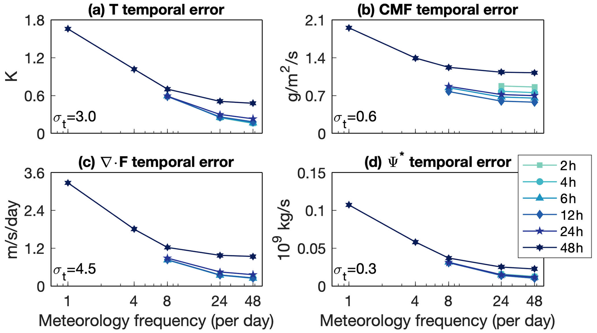
Figure 2 Globally and vertically averaged root-mean-square temporal error in (a) temperature, (b) convective mass flux, (c) EP flux divergence, and (d) the TEM streamfunction as a function of meteorology frequency (horizontal axis) and nudging timescale (see legend). For reference, the globally and vertically averaged temporal standard deviation of each field is shown in each panel.

Figure 3 As in Fig. 2 but for the root-mean-square spatial error, and the globally and vertically averaged spatial standard deviation of each field is shown in each panel.

Temporal and spatial errors in the convective mass flux decrease exponentially with increasing meteorology frequency but reach a minimum at a 12 h nudging timescale (Figs. 2b and 3b). At shorter and longer nudging timescales the error increases. For parameterized processes such as clouds, nudging presents a conundrum. Cloud heating will be built in to the reference meteorology temperature, so that nudging to the reference meteorology temperature will effectively perform some fraction of the convective heating via the nudging itself. It is indeed the case that the global convective mass flux erroneously weakens with decreasing nudging timescale (Fig. 4b), which in the tropics manifests as a robust decrease below 500 hPa (Fig. 5a, b). Orbe et al. (2017) similarly show that a CESM1(WACCM4) simulation nudged to Modern-Era Retrospective analysis for Research and Applications (MERRA) at a 5 h nudging timescale has a weakened convective mass flux relative to a simulation nudged to MERRA at a 50 h nudging timescale. There are time-average positive temperature nudging tendencies at the characteristic altitudes of shallow and deep convective heating that may be acting to suppress convection (Fig. 5c). Aloft, negative temperature nudging tendencies, which may be acting in lieu of cloud-top radiative cooling, scale with decreasing nudging timescale and are associated with increased convective mass flux. Nudging, especially at a timescale shorter than 24 h, incurs substantial and apparently unavoidable (Fig. 4b) penalties in convective mass flux.

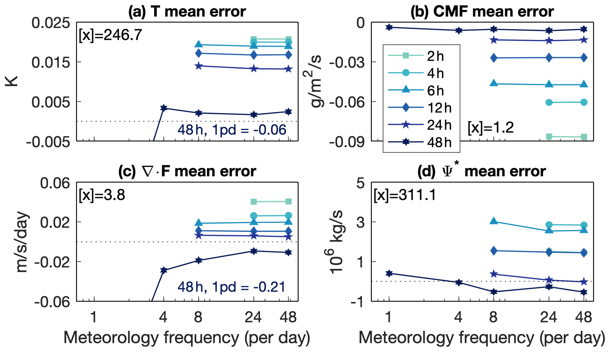
Figure 4 As in Fig. 2 but for the mean error, and the globally and vertically averaged absolute value of each field is shown in each panel.

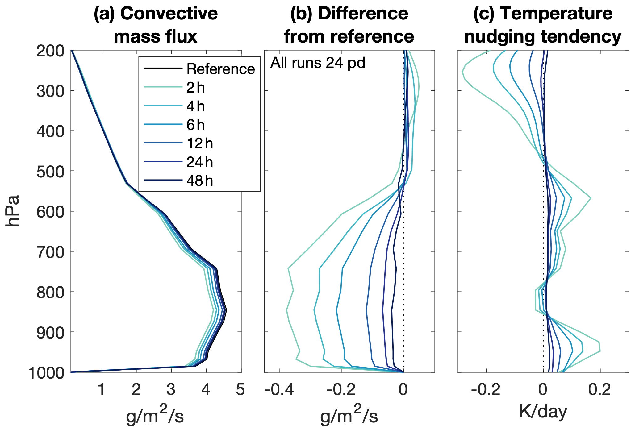
Figure 5 Tropical convective mass flux (a) mean and (b) difference from the reference meteorology, and (c) temperature nudging tendency for all nudging timescales at 24 meteorology updates per day. Average taken from 20^∘ S to 20^∘ N.

On the other hand, nudging at too long or short a timescale leads to clouds occurring at different times (Fig. 2b) and in different places (Fig. 3b) than the reference meteorology, even though it may result in minimal global mean error at the longest nudging timescale (Fig. 4b). While spatial and mean errors in the convective mass flux asymptote at approximately 10 % of the total variability, temporal errors asymptote at values equal to and larger than the variability.

The positive mean error of the EP flux divergence, indicating greater wave generation and wave drag, is consistent with the positive mean error in the TEM streamfunction (Fig. 4c, d). The tropical stratospheric upwelling velocity is an especially important measure of the residual circulation, as it diagnoses the net transport through the tropical tropopause layer and into the stratosphere. Tropical upwelling in the lower stratosphere increases with decreasing nudging timescale, with a peak increase of 3 %–5 % at a 2 h nudging timescale and no detectable difference at a 24 h nudging timescale (Fig. 6).

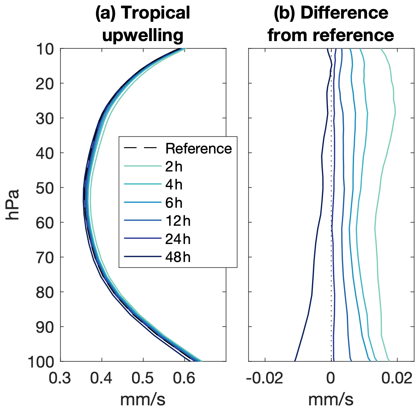
Figure 6 Tropical stratospheric upwelling (a) mean and (b) difference from the reference meteorology for all nudging timescales at 24 meteorology updates per day. Tropical stratospheric upwelling is defined as the area average of all annual mean upwelling vertical velocities at each vertical level.

5 Global errors in tracers

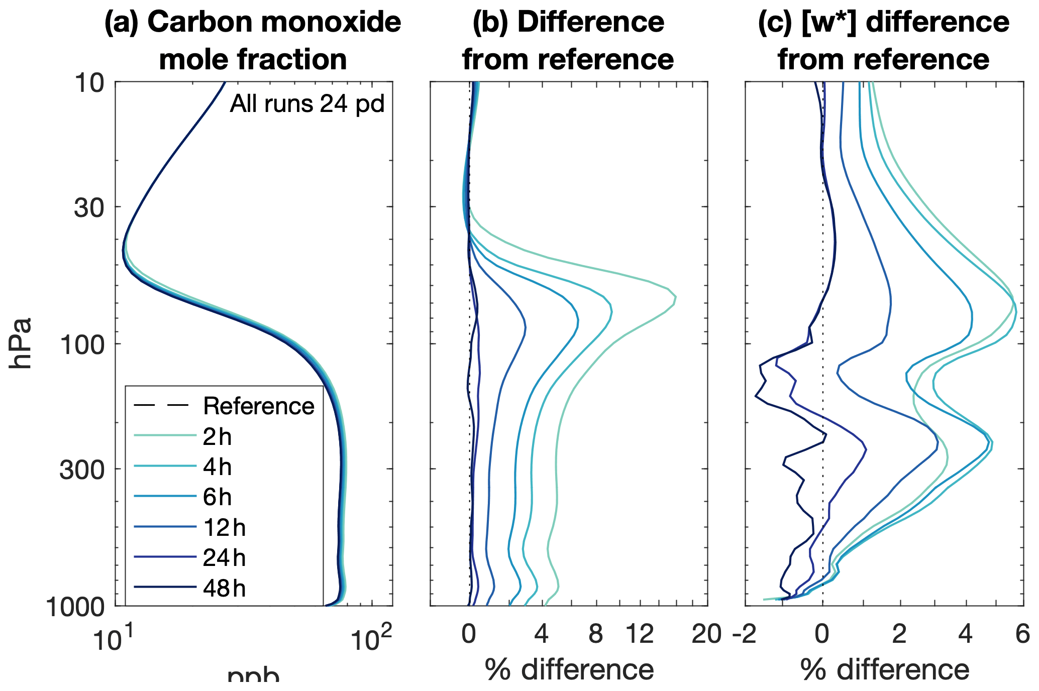
Errors in ozone and carbon monoxide mole fraction in the troposphere and stratosphere behave similarly to errors in the convective mass flux (Figs. 7 and 8), with a minimum in spatial and temporal errors at 12 to 24 h nudging timescales. While temporal errors are high at only the shortest and longest nudging timescales, spatial errors are especially high at nudging timescales shorter than 12 h. The temporal errors asymptote at around 10 %–25 % of the total variability, while spatial errors asymptote at a mere 0.1 %–5 %. This is probably due to the first-order influence of photochemistry on the global distribution of these tracers. Spatial error is a relatively strong function of timescale, while temporal error tends to scale more consistently with meteorology frequency.

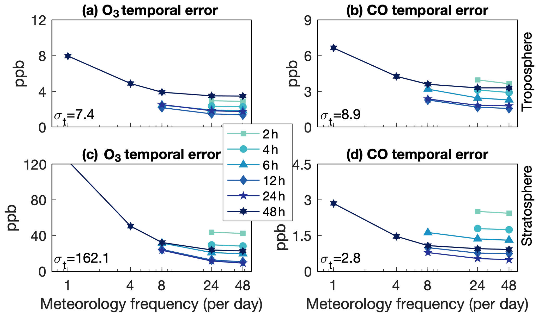
Figure 7 Globally and vertically averaged root-mean-square temporal error in tropospheric (a) ozone and (b) carbon monoxide and stratospheric (c) ozone and (d) carbon monoxide. For reference, the globally and vertically averaged temporal standard deviation of each field is shown in each panel.

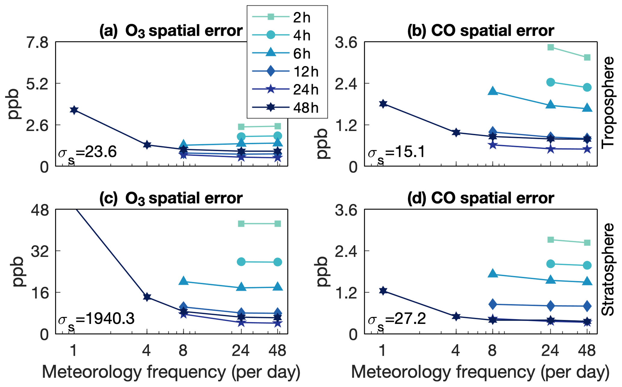
Figure 8 As in Fig. 7 but for the root-mean-square spatial error, and the globally and vertically averaged spatial standard deviation of each field is shown in each panel.

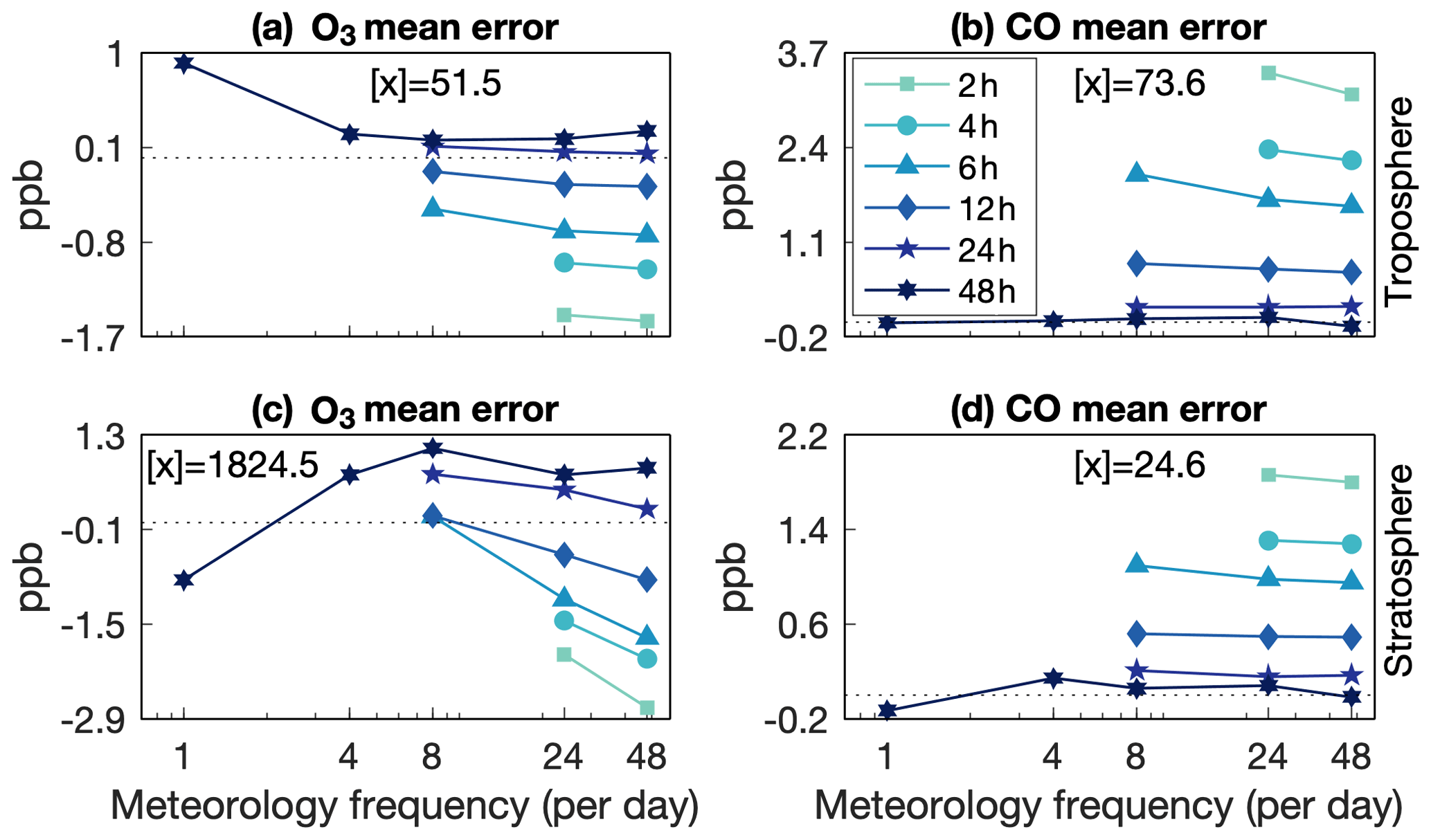
Figure 9 As in Fig. 7 but for the mean error, and the globally and vertically averaged absolute value of each field is shown in each panel.

The mean errors in tropospheric and stratospheric carbon monoxide and stratospheric ozone mole fraction decrease with increasing nudging timescale (Fig. 9a, b, d) and all but disappear at a 48 h nudging timescale. In both regions, carbon monoxide is biased low. Stratospheric ozone displays a unique dependence on meteorology frequency, although it is still also governed by the nudging timescale (Fig. 9c). As for the spatial and temporal errors, the mean error in stratospheric ozone also reaches a minimum at the 12–24 h nudging timescale. However, the mean errors are generally small, ranging from 5 % for stratospheric carbon monoxide to 0.1 % for stratospheric ozone.

These mean errors in the troposphere are surprising given the errors in the convective mass transport. Deep convection rapidly transports boundary layer air to the upper troposphere. This air is relatively low in ozone and relatively rich in carbon monoxide, such that convection acts to reduce upper tropospheric ozone (Folkins et al., 2002; Doherty et al., 2005; Voulgarakis et al., 2009; Paulik and Birner, 2012) and increase upper tropospheric carbon monoxide (Kar et al., 2004; Park et al., 2009). The weakening convective mass flux with decreasing nudging timescale (Fig. 5) should lead to elevated free-tropospheric ozone and reduced free-tropospheric carbon monoxide in the tropics. However, the opposite occurs, with reduced ozone and increased carbon monoxide throughout the whole troposphere and the lower stratosphere (Figs. 10 and 11). An alternative explanation is that the acceleration of the residual circulation with decreasing nudging timescale leads to anomalously negative ozone and anomalously positive carbon monoxide advection tendencies in the free troposphere, which propagate up though the tropical pipe (Figs. 10c and 11c). It is unclear why the broader but slower ascent by the residual circulation would exert a more dominant control than localized but more intense convective mass transport. It may be that changes in convective transport are more readily damped by horizontal advection than changes in zonal mean ascent.

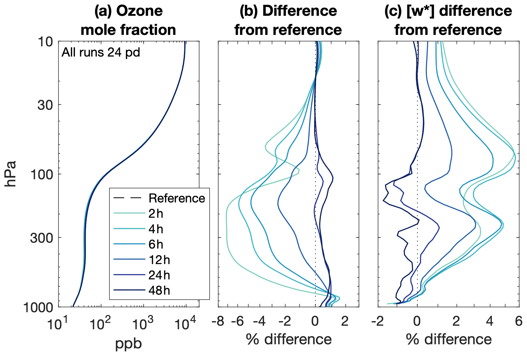
Figure 10 Tropical ozone (a) mean and (b) percent difference from the reference meteorology, and (c) residual vertical velocity for all nudging timescales at 24 meteorology updates per day. Average taken from 20^∘ S to 20^∘ N.

Figure 11 As in Fig. 10 but for carbon monoxide.

The serious impact of the nudging timescale and meteorology frequency on ozone and carbon monoxide warrants further investigation. Errors in the tropics are consistent with circulation differences rather than convective transport differences, so it seems reasonable to posit that differences in the resolved circulation are the dominant source of the error.

6 Errors in eddy-mean flow dynamics

The systematic variation of temporal, spatial, and mean errors with the nudging timescale and meteorology frequency means that they can be reliably described by appropriate regressions across the parameter space. While temporal and spatial errors in the circulation appear to be governed primarily by meteorology frequency (Figs. 2 and 3), temporal and spatial errors in ozone and carbon monoxide appear to be governed by meteorology frequency and the nudging timescale, respectively (Figs. 7 and 8). Mean errors in all fields are primarily governed by the nudging timescale (Figs. 4 and 9). Therefore, we will focus on the regression of temporal and spatial errors in the EP flux and its divergence and the TEM streamfunction on meteorology frequency, while we will focus on the regression of temporal and spatial errors in ozone and carbon monoxide on meteorology frequency and the nudging timescale, respectively. For all fields, we will focus on the regression of mean error on the nudging timescale. We will display the negative of all error regressions – that is, for decreasing nudging timescale and decreasing meteorology frequency.

To examine the structure of temporal and mean errors, we simply project the zonal mean root-mean-square temporal error or mean error in each simulation onto either the logarithm of meteorology frequency or onto a 1 standard deviation change in the nudging timescale (about 15 h). For examining spatial errors, we first project each field onto the time series of its spatial error to obtain a zonal mean map and then project the maps from each simulation onto either the logarithm of meteorology frequency or onto the nudging timescale. One can interpret the first regression as the change in temporal or mean error per change in either meteorology frequency or nudging timescale. The second regression is more nuanced, as it is not the spatial error that is regressed but instead the pattern in the physical field associated with variations in spatial error. The second regression should therefore be interpreted as the (erroneous) pattern in the physical field associated with either meteorology frequency or nudging timescale. It is useful only as a visualization of the structures that produce spatial error and vary with nudging parameters and not indicative of the change in the spatial error itself, which only has the dimension of time.

As meteorology frequency decreases, the temporal error in the TEM residual streamfunction increases in general proportion to the climatology (Fig. 12a). In the troposphere, temporal errors in the midlatitude Ferrel circulation, but not the Hadley cell, increase with decreasing meteorology frequency (Fig. 12a). The projection of TEM streamfunction spatial error is characterized by a single pole-to-pole, surface-to-stratopause cell (Fig. 12c), which suggests that the errors arise when the solstitial residual circulation is generally too strong and expansive in one hemisphere and too weak and contracted in the other. In the troposphere, spatial error is especially concentrated in the tropics and the storm tracks where there is moist diabatic ascent.

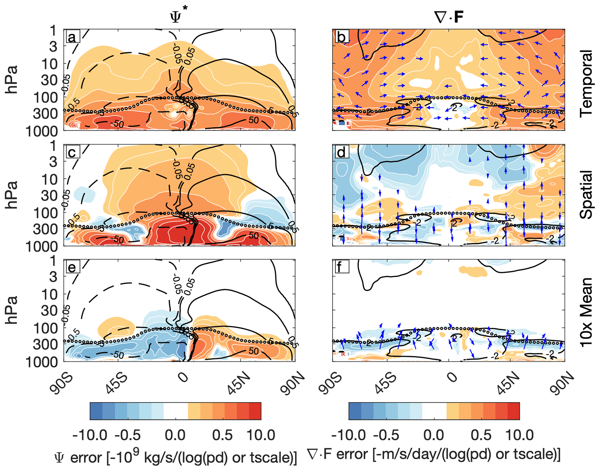
Figure 12 Negative of the projection of (a, b) root-mean-square temporal error, (c, d) root-mean-square spatial error, and (e, f) mean error in the (a, c, e) TEM streamfunction and (b, d, f) EP flux and divergence onto the (a, b, c, d) logarithm of meteorology frequency and (e, f) nudging timescale. Projection in shading (logarithmic scale), climatology in contours, and EP flux in vectors, scaled as in Edmon et al. (1980). In panels (a), (c), and (e) the climatological TEM streamfunction is contoured 0.05, 0.5, 5, and 50 × 10⁹ kg per second, with positive values solid and negative values dashed. In panels (b), (d), and (f) the climatological EP flux divergence is contoured every 2 m per second per day, with negative values solid. The tropopause is shown by the black and white dotted contour.

As meteorology frequency decreases, the temporal errors in the stratospheric EP flux divergence increase poleward of the climatological divergence and deep within the polar vortices, associated with errors in the meridional propagation of Rossby waves (Fig. 12b). In the upper stratosphere the meridional position of the peak EP flux divergence dominates the spatial error in the Northern Hemisphere, while it is instead dominated by the total magnitude of the EP flux divergence in the Southern Hemisphere (Fig. 12d). In both hemispheres, this error is governed by a vertical redistribution of wave activity rather than by changes in meridional propagation. In the troposphere, temporal errors in the EP flux divergence increase with decreasing meteorology frequency in the extratropics in proportion to the climatology. There is no planetary-scale structure to the spatial error in the troposphere, although it appears roughly antisymmetric about the Equator (Fig. 12d). As in the stratosphere, this error is governed primarily by a vertical redistribution of wave activity.

In the troposphere the TEM streamfunction and EP flux divergence/convergence are invigorated by decreasing the nudging timescale (Fig. 12e, f). The invigoration of the stratospheric TEM streamfunction is limited to the shallow branch of the circulation, with the error rapidly tapering off above 50 hPa. Global average mean errors in the circulation (Fig. 4c, d) are therefore reflective of the mean error almost everywhere in the troposphere but virtually nowhere in the stratosphere.

The physical coupling between the wave-driven TEM streamfunction and EP flux divergence raises the question of which aspect of the circulation – the zonal mean or the eddies – is the source of their errors (Figs. 2c, d; 3c, d). A simple diagnostic is to “swap” either the zonal mean or eddy fields from the reference meteorology into the calculation of the TEM streamfunction and EP flux divergence in the nudged simulations and recalculate the errors. The reduction in error between the swapped and non-swapped simulations measures the impact of the swapped field on the error. It is only diagnostic and does not entertain any feedbacks between the eddies and the mean flow.

Temporal, spatial, and mean errors in the TEM streamfunction are overwhelmingly due to the Eulerian-mean part of the circulation, while the errors in the EP flux divergence are entirely due to the eddy fields (Fig. 13). The eddy fluxes that comprise the EP flux divergence are merely scaled by their projection onto angular momentum and static stability, so it is not so surprising that the Eulerian mean contribution is negligible. It does seem surprising that the Eulerian mean dominates the errors in the TEM streamfunction though. While the correction for the eddy recirculations is not a dominant component of the TEM streamfunction except in the extratropics, the errors they introduce are apparently vanishingly small. This result instead points to temperature nudging (Fig. 5c) directly invigorating the Eulerian mean part of the circulation (Fig. 6, and see also Miyazaki et al., 2005; Akiyoshi et al., 2016).

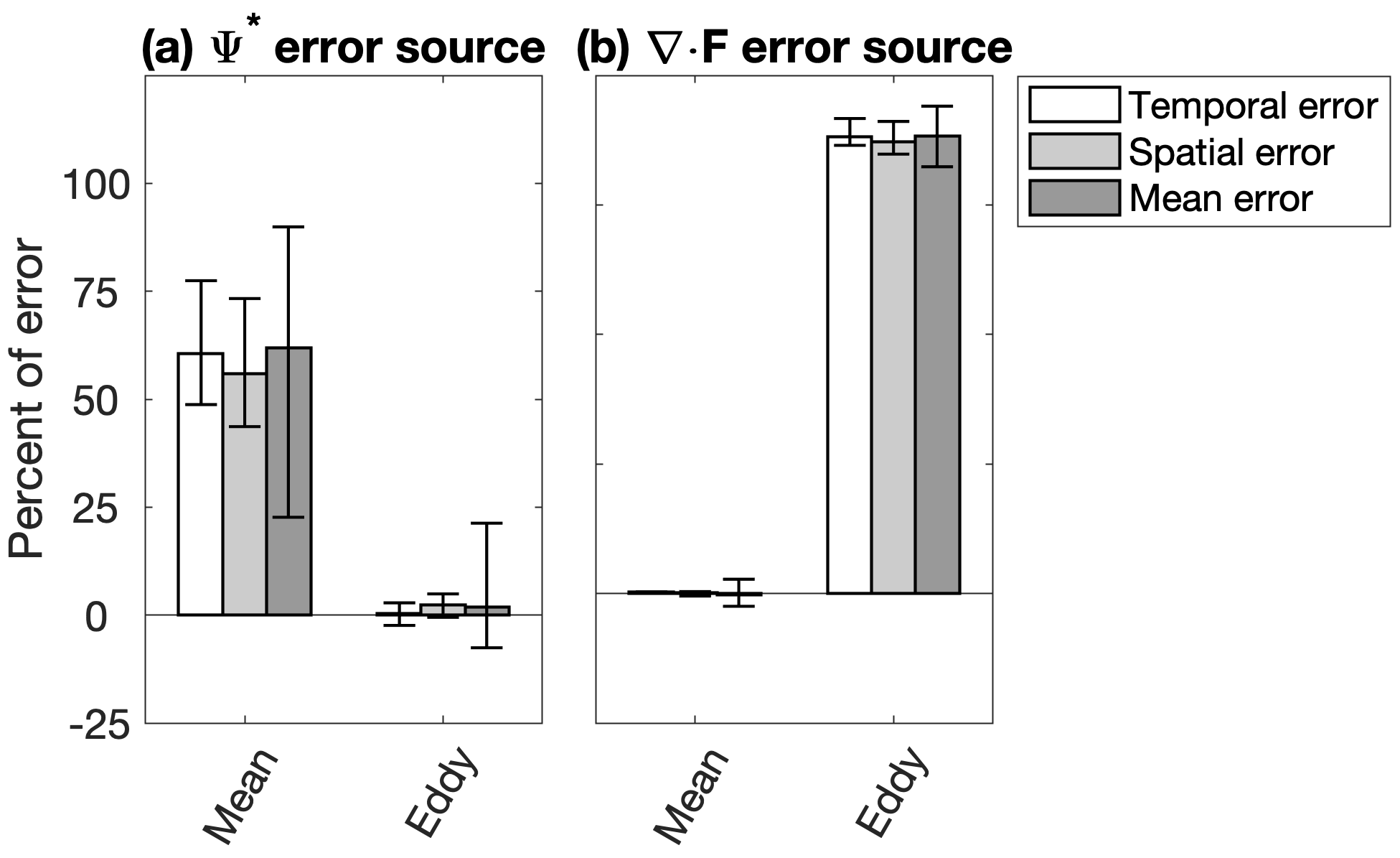
Figure 13 Percent of the temporal, spatial, and mean error in the (a) TEM streamfunction and (b) EP flux divergence attributable to the zonal mean or eddy fields. Whiskers indicate the maximum and minimum across all nudging simulations.

7 Errors in ozone and carbon monoxide and their transports

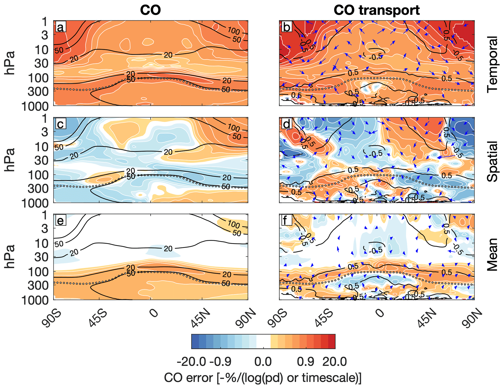
These errors in the dynamics project strongly onto ozone (Figs. 14 and 15) and carbon monoxide (Figs. 16 and 17). Here we sum the eddy and residual circulation fluxes and convergences on the right hand side of Eq. (11) and perform the same regressions as before. However, to more directly assess the impact of each type of transport error on ozone and carbon monoxide, we multiply the error in the combined TEM residual flux and TEM eddy flux convergence by the e-folding timescale of the corresponding tracer. The timescales are estimated by determining the lag at which each tracer's autocorrelation drops to $\mathrm{1}/e$ in the reference run. The e-folding timescale for ozone ranges from 5 d in the tropical upper troposphere and lower stratosphere to 70 d in the extratropical stratosphere, while for carbon monoxide it ranges from 30 d in the tropical upper troposphere and lower stratosphere to 70 d in the extratropical stratosphere (see Fig. S4). Both of these timescales have substantial vertical and horizontal structure.

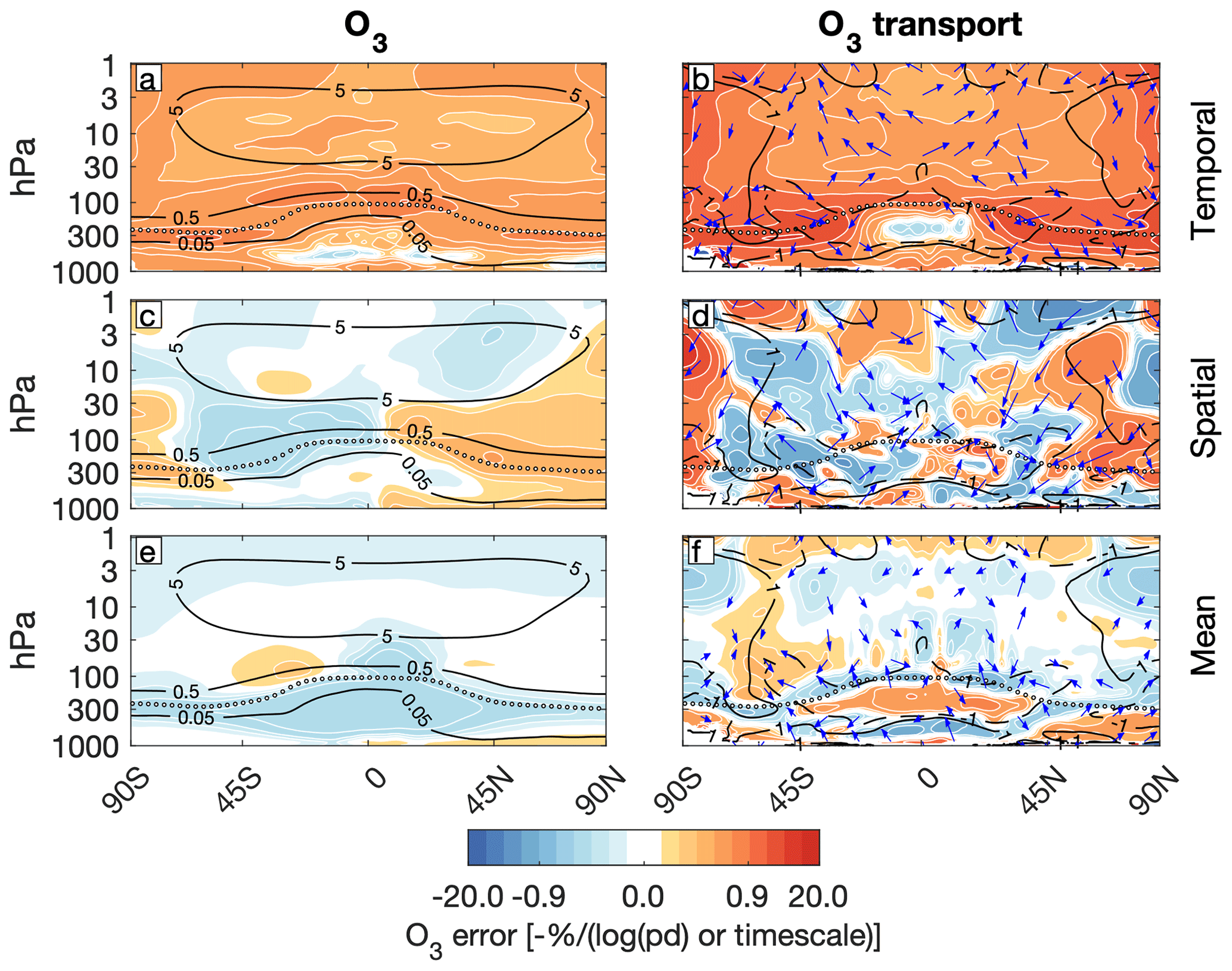
Figure 14 Negative of the projection of (a, b) root-mean-square temporal error, (middle row) root-mean-square spatial error, and (e, f) mean error in (a, c, e, shading) the ozone mole fraction and (b, d, f, vectors) the combined TEM residual circulation and eddy ozone flux and (shading) convergence onto the (a, b) logarithm of meteorology frequency and (c, d, e, f) nudging timescale. Climatology in contours in (a, c, e) parts per thousand and (b, d, f) percent per day, with negative values dashed. The tropopause is shown by the black and white dotted contour.

Figure 15 As in Fig. 14 but for carbon monoxide and based on the projections in the right column of Fig. 16.

.

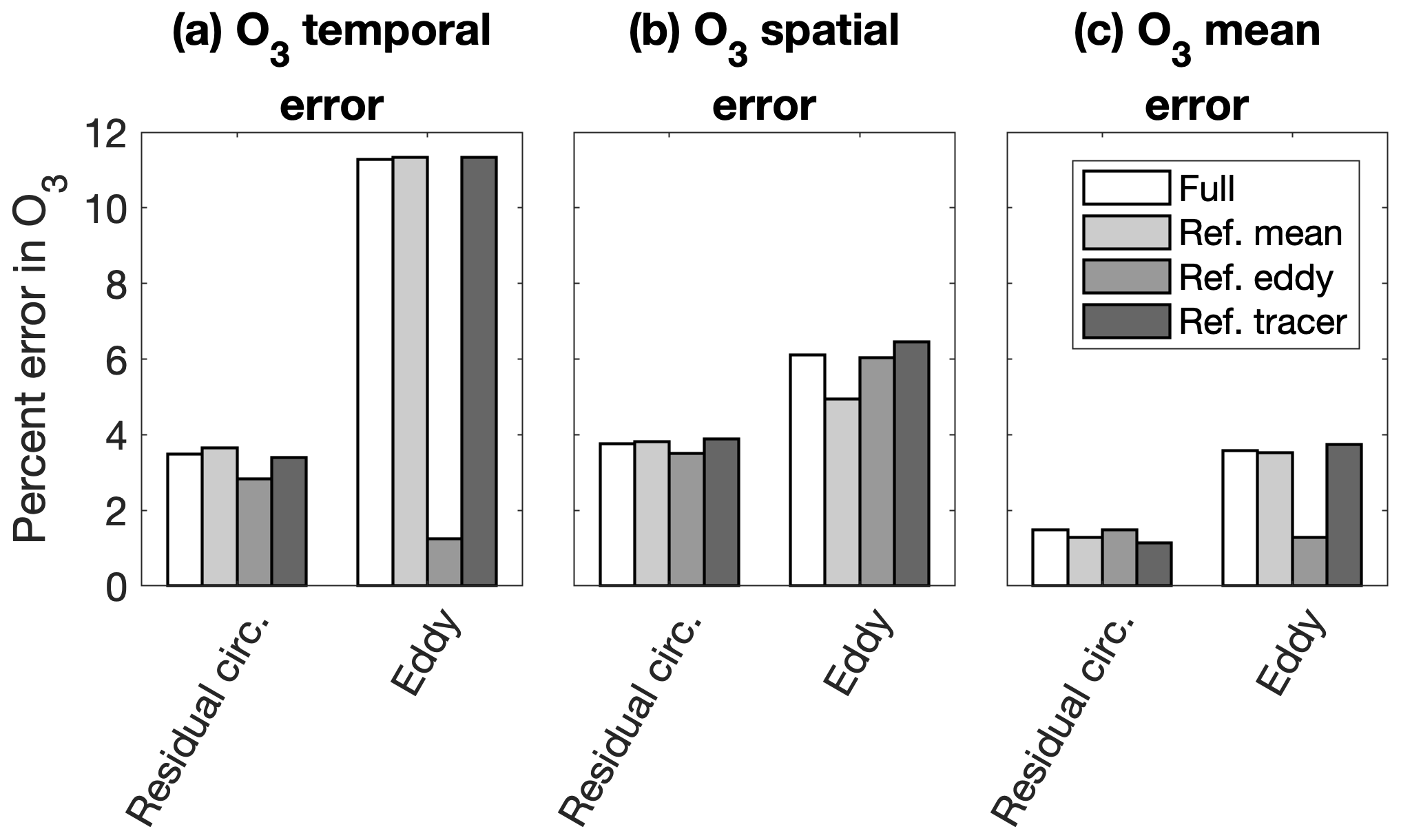
Figure 16 Global average (a) root-mean-square temporal error, (b) root-mean-square spatial error, and (c) sign-adaptive mean error in ozone attributable to the TEM residual circulation and TEM eddy flux convergences, based on the projections in the right column of Fig. 14

Figure 17 As in Fig. 16 but for carbon monoxide.

With decreasing meteorology frequency, temporal errors in ozone and carbon monoxide peak at greater than 1 % and 10 % of the climatology, respectively, in the upper troposphere and lower stratosphere and in the polar stratosphere (Figs. 14a and 15a). This pattern is mirrored by an increase in temporal errors in the ozone and carbon monoxide flux convergences with decreasing meteorology frequency (Figs. 14b and 15b). As these errors reflect the temporal error in the EP flux divergence (Fig. 12b), they appear consistent with local errors in eddy mixing.

However, there is a strong signal in the temporal error in the ozone and carbon monoxide fluxes, but not convergences, in the tropical upper stratosphere. This implicates the deep branch of the residual circulation, which acts non-locally to accumulate errors in tracers along the Equator-to-pole transport pathway, both up and down the tracer gradient.

Ozone and carbon monoxide spatial errors associated with nudging timescale peak at up to 0.5 % in the upper troposphere and lower stratosphere (Figs. 14c and 15c). In the upper troposphere and lower stratosphere, this hemispherically asymmetric pattern is loosely related to the spatial errors in their transports (Figs. 14d and 15d). Erroneously high ozone in one hemisphere is associated with erroneous downward and equatorward transport from the middle stratosphere, while it is the opposite in the other hemisphere. Likewise, erroneously low carbon monoxide in one hemisphere is associated with erroneous flux divergence, and vice versa in the other hemisphere.

In the upper stratosphere, though, the spatial errors in ozone and carbon monoxide are out of phase with their transport errors, which may indicate that the transport errors follow from the tracer errors. For example, the pattern of erroneously low midlatitude and high polar upper-stratospheric ozone in the Northern Hemisphere is associated with a tripole of enhanced ozone flux divergence and flux convergence. Similarly, enhanced carbon monoxide in the polar upper stratosphere in the Northern Hemisphere is associated with a dipole of enhanced flux divergence and convergence. Both of these flux divergence/convergence patterns are associated with downward transport from the mesosphere, where the circulation is unconstrained by the specified dynamics scheme.

Decreasing nudging timescale leads to a reduction in ozone and increase in carbon monoxide throughout the troposphere (Figs. 14e and 15e), with the largest changes in the tropics. The reduction in ozone is associated with weakened vertical transport in the troposphere relative to the climatology (Fig. 14f) and greater negative transport tendencies throughout the lower stratosphere as the erroneously ozone-poor air is spread out along the tropopause. There is a region of erroneous downward and poleward transport in the Southern Hemisphere that seems to be associated with the invigoration of the shallow branch of the TEM residual streamfunction with decreasing nudging timescale (Fig. 12e). It does not seem to materially impact the scaling between nudging timescale and stratospheric ozone though (Fig. 9c). The increase in carbon monoxide is consistent with an upward shift in transport, with too much transport out of the troposphere into the lower stratosphere (Fig. 15f).

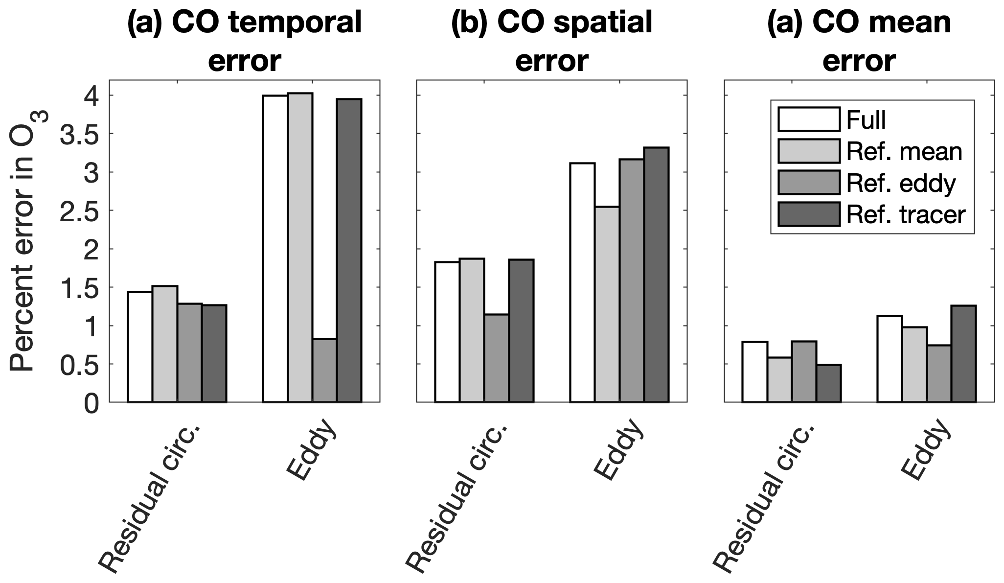
We can quantify the sources of these errors in transport by using the same “swapping” technique as before. Here, we will swap in the reference zonal mean transport terms, the eddy transport terms, and the zonal mean tracer field (separately from the other zonal mean terms) and recalculate the transport terms, the regression, and the conversion of the regression into an ozone and carbon monoxide error using the ozone and carbon monoxide e-folding timescales.

The temporal error in transport is overwhelmingly due to eddy transport, which drives a global average 10 % error in ozone and 4 % error in carbon monoxide (Figs. 16a and 17a, white bars). Spatial and mean errors due to transport are more balanced between residual circulation and eddy transport (Figs. 16b–c and 17b–c, white bars). Ozone and carbon monoxide transport temporal errors and ozone transport mean error are reduced only when using the reference eddy fields. Because of the strong covariance between the temporal error in ozone and carbon monoxide transport and the temporal error in the EP flux divergence (Figs. 14b, 15b, and 12b), we can infer this is probably due to errors in the eddy circulations themselves.

There are several other small reductions in error, but none are especially noteworthy, and no diagnostic swap reduces the errors in residual circulation ozone transport. In general, then, the errors in ozone and carbon monoxide mole fractions cannot be understood as local errors. Instead, the global circulation acts to accumulate ozone and carbon monoxide errors along transport pathways.

8 Conclusions and discussion

Through an analysis of 18 CESM2 (WACCM6) specified dynamics simulations over the course of one simulated year, we have found the following.

1. Meteorology frequency is the primary contributor to temporal and spatial errors in the resolved tropospheric and stratospheric circulation.

   • a.

     As meteorology frequency increases, spatial and temporal error decreases.

   • b.

     At a given meteorology frequency, nudging timescales shorter than 24–48 h produce the lowest error.

2. Meteorology frequency is the dominant contributor to temporal error in ozone, carbon monoxide, and convective mass flux, while nudging timescale is the primary contributor to their spatial error.

   • a.

     As meteorology frequency increases, temporal error decreases.

   • b.

     As nudging timescale increases, spatial error generally decreases, but it reaches a minimum at a 12–24 h nudging timescale.

3. The nudging timescale is the primary contributor to mean error in all fields, with the lowest mean error at 24–48 h nudging timescales.

Taken together, these results suggest that the maximum meteorology frequency possible, with a moderate nudging timescale of 12–24 h, is an optimal configuration for CESM2 (WACCM6) 110-level specified dynamics simulations that balances the three different types of error across all of these fields.

Errors in tracers are generally the lowest in emission/production regions and highest at the end of characteristic transport pathways (Fig. 18). Convection and the tropospheric residual circulation create errors in ozone and carbon monoxide and accumulate them in the upper troposphere and lower stratosphere through rapid overturning, similar to a conveyer belt. These errors propagate upward into the stratosphere via the residual circulation and get mixed horizontally by Rossby waves along the tropopause. Above this level, errors are rapidly damped by photochemistry. Similarly, the deep branch of the residual circulation creates errors in ozone downstream of photochemical production in the tropical stratosphere and accumulates them in the polar stratosphere, where they are redistributed and accentuated by errors in Rossby wave transport. Because the dynamics in the mesosphere cannot be reliably constrained without substantial instabilities, the photochemical production and downward transport of carbon monoxide through the mesosphere and into the upper stratosphere by the residual circulation (Minschwaner et al., 2010; Garcia et al., 2014) result in substantial errors in polar stratospheric carbon monoxide.

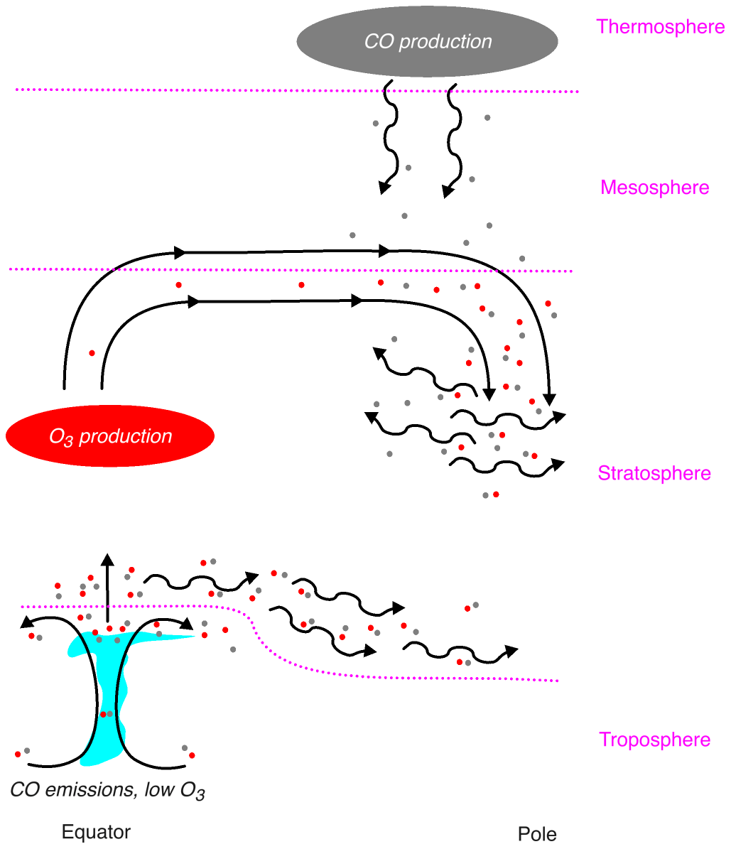
Figure 18 Schematic of transport errors produced by the specified dynamics scheme. The residual circulation is illustrated by the steady black arrows, while the eddies are illustrated by the squiggly black arrows. Convection is shown by the light blue cloud, while photochemical production regions are shown by the large bubbles for (red) ozone and (gray) carbon monoxide, with the concentration indicating the severity of the error. Errors are shown by the small dots for (red) ozone and (gray) carbon monoxide. Dotted lines delineate the tropopause and stratopause.

As this model configuration is computationally expensive, our analysis only spans 1 year due to the practical need to sweep enough of the phase space of nudging parameters. We therefore believe that while the errors in the circulation are probably close to the value we would infer from longer simulations, the errors in the tracer fields should be seen as a lower bound, especially in the middle atmosphere. Circulation errors integrated over at least the stratospheric age of air, which ranges from 1 to 5 years (Engel et al., 2017; Ploeger et al., 2019), could lead to sustained increases in tracer error. It also may be the case that production and loss processes are strong enough to damp this hypothetical increase. As a final caveat, the reference simulation generated a sudden stratospheric warming, which may have produced some of the hemispherically asymmetric structures in the error (Figs. 12, 14, and 15).

The relatively strong dependence of errors in chemical tracers and clouds on both nudging timescale and meteorology frequency is especially concerning because specified dynamics simulations, by their nature, are intended to constrain the circulation and isolate its role in chemical weather and climate. Few of the tracer errors can be tied to particular and local processes. However, the high sensitivity of these errors suggests that any modeling interventions could have major impacts.

To gain some practical insight into how these results might generalize to the case where the reference meteorology is produced by a different modeling system, we performed a subset of specified dynamics simulations in which we nudged CESM2(WACCM6) to NASA's 3-hourly operational GEOS meteorology from 1 January 2018 through 31 December 2018. These simulations had a nudging timescale of 12 h and a meteorology frequency of 4 per day, a nudging timescale of 12 h and a meteorology frequency of 8 per day, and a nudging timescale of 48 h and a meteorology frequency of 8 per day (Fig. 19). We consider the configuration with a nudging timescale of 12 h and a meteorology frequency of 8 per day as the best-case configuration, while we expect the other two configurations to produce higher errors. For these simulations, CESM2(WACCM6) is still run on its native horizontal and vertical grid, while GEOS U, V, and T are gridded to the CESM2(WACCM6) grid before nudging.

Figure 19 Global average temporal, spatial, and mean errors in (a) temperature, (b) convective mass flux, (c) Eliassen–Palm flux divergence, and (d) TEM residual streamfunction in specified dynamics simulations nudged to NASA GEOS5 meteorology, for three different nudging parameter configurations. Numbers under each set of bars indicate the global average temporal or spatial standard deviation or mean value for each field.

The temperature (Fig. 19a) and Eliassen–Palm flux divergence (Fig. 19c) errors generally scale as they do when the model is nudged to itself, with errors increasing with increasing timescale and decreasing meteorology frequency. The increase in mean error with nudging timescale probably reflects a difference between the climatologies of CESM2(WACCM6) and GEOS5, with CESM2(WACCM6) drifting toward its own climatology at a 48 h nudging timescale.

Errors in the convective mass flux (Fig. 19b) and TEM residual streamfunction (Fig. 19d) are insensitive to variations in the nudging parameters. These configurations are centered on the minimum in error when CESM2(WACCM6) is nudged to itself (Figs. 2–4), so it could be that a greater variation in the parameters is needed to elicit distinct behavior. However, as before the errors are high relative to the background variability. The inability of the specified dynamics scheme to effectively constrain convection and the meridional circulation to their values in the input meteorology reflects previous work (Orbe et al., 2017, 2018; Chrysanthou et al., 2019) and presents a major challenge, as both contribute to global transport.

It is worth asking just how much we can reduce the errors in specified dynamics schemes based on a linear relaxation of winds and temperatures. Nudging potential vorticity, rather than the individual components of the wind, may better constrain the divergent circulation (Li et al., 1998; Pulido, 2014) and curtail erroneous circulation responses (DeWeaver and Nigam, 1997). It would still need to be paired with temperature nudging to ensure a proper representation of temperature-dependent chemistry, water vapor, and microphysics.

If the relative magnitude of the nudging tendencies at a given time step can be used as a proxy for the instability of the current atmospheric state, analogous to bred vectors (Cai et al., 2003), our current constant-timescale linear relaxation could be modified into a flow-adaptive timescale. The flow-adaptive timescale could be set to nudge the meteorology at a fast timescale only when absolutely necessary, as meteorology errors are relatively insensitive to nudging timescales faster than 24 h. It could also be made aware of active convection and either reduce the nudging timescale accordingly or switch off temperature nudging to allow the convective physics the freedom to modify the temperature field and transport constituents. Flow-adaptive nudging of potential vorticity and temperature may provide a tractable solution for further reducing errors in tracers and clouds, while still sufficiently constraining the circulation.