High-resolution mapping of regional traffic emissions using land-use machine learning models

On-road vehicle emissions are a major contributor to significant atmospheric pollution in populous metropolitan areas. We developed an hourly link-level emissions inventory of vehicular pollutants using two land-use machine learning methods based on road traffic monitoring datasets in the Beijing–Tianjin–Hebei (BTH) region. The results indicate that a land-use random forest (LURF) model is more capable of predicting traffic profiles than other machine learning models on most occasions in this study. The inventories under three different traffic scenarios depict a significant temporal and spatial variability in vehicle emissions. NO_x, fine particulate matter (PM_2.5), and black carbon (BC) emissions from heavy-duty trucks (HDTs) generally have a higher emission intensity on the highways connecting to regional ports. The model found a general reduction in light-duty passenger vehicles when traffic restrictions were implemented but a much more spatially heterogeneous impact on HDTs, with some road links experiencing up to 40 % increases in the HDT traffic volume. This study demonstrates the power of machine learning approaches to generate data-driven and high-resolution emission inventories, thereby providing a platform to realize the near-real-time process of establishing high-resolution vehicle emission inventories for policy makers to engage in sophisticated traffic management.

1 Introduction

Rapid social and economic growth in China has driven the development of road transportation systems and mobility services over the past few decades. This macrotrend also aligns with the faster pace of urban expansion and agglomeration, creating higher travel activities that are not only caused by urban commuting but also by intercity connections. Consequently, on-road transportation systems have resulted in substantial challenges regarding traffic congestion, carbon emissions, air pollution, and land-use issues (Uherek et al., 2010; Waddell, 2002; Chapman, 2007). To address traffic-related air pollution issues, previous studies have developed link-level emission inventories for metropolitan areas or their urban cores. Notably, more studies have recognized the considerable environmental impact of nonlocally registered vehicles, especially nonlocal heavy-duty diesel trucks (HDDTs) used for regional freight purposes. For example, nonlocal HDDTs are estimated to contribute nearly 30 %–40 % of the total on-road emissions of nitrogen oxides (NO_x) and fine particulate matter (PM_2.5), which is greater than the contribution of the 5 million local passenger cars (Wang et al., 2011; Yang et al., 2019a). Undoubtedly, for transportation hubs, such as Beijing, we see a clear need to support policymaking by enlarging road emission inventories to the multiprovince level in order to improve the management of transportation emissions.

The technological evolution of intelligent transportation systems has facilitated emission inventories for megacities. For example, Gately et al. (2017) applied speed data from mobile phones and vehicles gathered using GPS (global positioning system) to map the emission fluxes from vehicles in the Greater Boston region. In addition to such trajectory data (Sun et al., 2018), open-access traffic congestion indexes could also be derived from navigation companies or municipal government agencies to dynamically estimate road speeds. For traffic volume and fleet mix, radio frequency identification (RFID) and traffic cameras are capable of reporting detailed vehicle counts using license plate numbers (Zhang et al., 2018). These real-world traffic datasets are useful for elucidating temporal and spatial variations in traffic emissions. However, we are still confronted with a few challenges with respect to constructing multiprovince, link-level emission inventories utilizing methods that are applicable to smaller research domains. First, the annual averaged daily traffic (AADT) data, for example, which could be assessed from the US Federal Highway Administration, typically use the traffic profiles of a select portion of a roadway system (i.e., “sample panel”) to represent the “full extent” of the system. Second, simple assumptions and empirical adjustments of vehicle kilometers traveled (VKT) are often used to downscale state-level or national-level AADT profiles to traffic patterns of specific counties (Gately et al., 2015). Both of these factors could result in estimates of the spatial variations in traffic volume that may not represent real-world patterns. Furthermore, the AADT datasets are updated every year according to the annual submission from all states. Therefore, the AADT datasets could support the average analysis of seasonal or day-of-the-week variations (McDonald et al., 2014) but are limited to reflecting emissions in a quasi-dynamic fashion (e.g., hourly).

Traffic demand modeling is a useful complement to measurements and simple empirical downscaling, and it has been utilized to assist in the development of emission inventories (Gately et al., 2017; Zhang et al., 2018). However, transportation simulation methods are often time-consuming. The machine learning method represents a faster complementary approach to estimating traffic flows in a particular context compared with full traffic demand modeling, and it is also more able to adapt to local conditions than simpler empirical approaches.

The research domain of this study, the Beijing–Tianjin–Hebei (BTH) region (see Fig. S1), geographically covers three provincial-level administrative regions with a total land area of 217 000 km². As the national political center, the BTH region has developed the busiest freight system in northern China but has also suffered from the worst air quality since the 2000s. We utilized hourly traffic profiles, including volume, speed, and fleet mix obtained from the governmental intercity highway monitoring network, to pioneer land-use machine learning methods for developing link-level emission inventories. The methodology can potentially be used to map traffic characteristics on a larger scale (at the national level) or to deal with real-time urban traffic data streams that need to overcome the challenges of computational accuracy and efficiency.

2 Methodology and data

2.1 Research domain and emission calculation

The government traffic monitoring datasets mainly cover main intercity highways, such as expressways, national highways, and provincial highways. Notably, we did not include urban sections or minor roads in the research domain because the traffic profiles of these roads were administered by local governmental agencies. The network of intercity main roads in the BTH region has a total length of 50 660 km, including 18 824 km of expressways, 8989 km of national highways, and 22 847 km of provincial highways (see the definition of road types in Table S1). There were 22.38 million registered vehicles (motorcycles excluded) in the entire region as of 2017, with an average annual growth rate of 7 % since 2013. In addition, freight trucks for the mass transportation of coal and steel from other provinces pass through the BTH region in very large numbers because this region accounts for approximately one-quarter of the total steel production in China.

The emissions of primary vehicular pollutants (carbon monoxide, CO; total hydrocarbon, THC; nitrogen oxide, NO_x; fine particulate matter, PM_2.5; and black carbon, BC) were calculated using a high-resolution method in a temporal and spatial framework. A link-level emission inventory modeling framework, called EMBEV-Link (Link-level Emission factor Model for the BEijing Vehicle fleet), was used to complete the emission calculation (Yang et al., 2019a). For each road link, hourly emissions are the product of the traffic volume, link length, and speed-dependent emission factors (see Eq. 1).

$$\begin{array}{}\text{(1)}& E_{\mathrm{h},j,\mathrm{l}}={\sum }_t{\mathrm{EF}}_{\mathrm{c},j}\left(v\right)\times {\mathrm{TV}}_{\mathrm{c},\mathrm{h},\mathrm{l}}\times L_{\mathrm{l}},\end{array}$$

where $E_{\mathrm{h},j,\mathrm{l}}$ is the total emission of pollutant j on road link l at hour h, in units of grams per hour (g h⁻¹); EF_c, j(v) is the average emission factor of pollutant j for vehicle category c at speed v, in units of grams per kilometer (g km⁻¹); TV${}_{\mathrm{c},\mathrm{h},j}$ is the traffic volume of vehicle category c on road link l at hour h, in units of vehicles per hour; and L_l is the length of road link l, in units of kilometers (km). According to the resolution of traffic mix data, six vehicle categories were defined, namely light-duty passenger vehicles (LDPVs), medium-duty passenger vehicles (MDPVs), heavy-duty passenger vehicles (HDPVs), light-duty trucks (LDTs), and heavy-duty trucks (HDTs) (see Table S2). In contrast to the city-scale emission inventories, we did not separate the traffic volume of transit buses and taxis from the HDPVs and LDPVs, respectively. Additionally, motorcycles were not included because it was difficult to observe them on these intercity highways. For each vehicle category, speed-dependent emission factors were developed based on the EMBEV model. The EMBEV model embodied the detailed fleet configurations based on vehicle registration data, which were developed based on thousands of in-lab dynamometer tests and hundreds of on-road tests (Zhang et al., 2014). Since 2015, this model has become the archetype of the official National Emission Inventory Guidebook in China (Wu et al., 2016, 2017). Based on the EMBEV model, this study updated the BTH emission database, taking full account of the differentiated vehicle emission characteristics of Beijing, Tianjin, and Hebei. The main influencing factors include the implementation timetable of vehicle emission standards, the fuel quality, the intensity of in-use vehicle supervision, and the proportion of high-emission vehicles, among others. Figure S2 shows the fleet-average emission factors of CO, NO_x, and BC for LDPVs and HDTs estimated by the updated EMBEV model in Beijing, Tianjin, and Hebei. As the traffic monitoring stations cannot obtain the emission standard information of the vehicle, the proportions of vehicles with a specific emission standard and the vehicle age/mileage (used to estimate mileage deterioration of emissions) were assumed to be consistent with the default fleet composition data in the EMBEV model. We also made adjustments based on the restriction policy, such as HDTs older than the China III standard are not allowed to drive within the Fifth Ring Road in Beijing. Figure S3 presents speed-dependent emission factors modified by different regions representing the traffic configurations (e.g., fuel type, emission standard, and vehicle size) and operating conditions (e.g., fuel quality) estimated for the calendar year of 2017. Evaporative THC emissions were not included in the current EMBEV-Link model because we were limited to spatially specifying the evaporative off-network emissions.

2.2 Traffic scenarios under various transportation management schemes

Three traffic scenarios were generated as inputs to the EMBEV-Link model in order to observe the impact of major transportation management schemes: scenario Weekday (S1), which represented the average traffic patterns during weekdays (Monday to Friday) with regular driving patterns; scenario Weekend (S2), which represented the average traffic patterns on weekends (Saturday and Sunday), possibly with more leisure travel; and, scenario Restriction (S3), which represented the traffic patterns under special restrictions. The Chinese government has launched comprehensive action to alleviate air pollution during serious pollution episodes. For the on-road sector, transportation restrictions are implemented on polluted days when the PM_2.5 concentrations or air quality index (AQI) are forecasted to be higher than certain thresholds. As one of the most polluted regions in China, the BTH region has implemented a package of traffic control measures, especially during winter, which has the worst meteorological conditions for pollution dispersion. In this study, the Restriction scenario (S3) estimated the real-world traffic patterns during a special week, from 4 to 8 November 2017, that experienced serious haze pollution. More extensive bans than usual were adopted during the abovementioned week, and coal-related freight trucks and high-emission vehicles (e.g., gasoline cars in compliance with pre-China II standards) were restricted from many roads in the BTH region; thus, the traffic composition (especially with respect to the configuration of the emission standard) would be adjusted accordingly in S3. In contrast to the averaged diurnal patterns in S1 and S2, hourly emissions were continuously estimated throughout the period with traffic restrictions.

2.3 Generating dynamic traffic profiles based on land-use machine learning models

2.3.1 Data collection

The input data for model development in this study mainly included traffic data and land-use data. An overview of the data used to train the land-use machine learning models is given in Table S3 and detailed below.

Traffic data

The Chinese Ministry of Transport has established nationwide networks to monitor intercity traffic conditions (Yang et al., 2019a; Zhang et al., 2018). Twenty-four-hour diurnal traffic profiles, including the volume, speed, and fleet mix, were obtained from 848 intercity highway sites in the BTH region (see Fig. S1). The hourly traffic profiles of a whole week (20 to 27 of the month) were collected in January, April, July, and November in 2017 in order to represent the average scenarios (S1 and S2). For S3, we further collected the hourly profiles from a special week (specifically, 5 and 6 November) that experienced traffic restrictions. Figure S4 shows the distribution of the annual average daily traffic profiles used to train the models in order to establish their capability to predict the spatial distribution of these traffic profiles. Notably, the monitoring data of the traffic volume could not separate the LDPVs and MDPVs from the light- to medium-duty passenger vehicles (LMDPVs) on the whole. Therefore, we assembled two categories when predicting the traffic volume and separated the predicted traffic volume values according to the estimated total vehicle activity (i.e., registered population × annual VKT).

Land-use data

As land-use machine learning models have rarely been used to develop traffic emission inventories, we selected candidate spatial predictors based on previous research on air pollution concentration predictors (Hoek et al., 2008; Lee et al., 2017). Many of these predictors, such as the population density, road density, and distance from transportation facilities (e.g., airports and transit stations), are expected to affect traffic activities as well. The potential predictor variables were divided into two groups: (1) variables representing a point value and (2) variables representing the cumulative values of an area (buffer variables). The buffer variables were represented as a density value (standardized by the buffer area). In total, 139 spatial predictor variables (see Table S3) regarding the land-use data were calculated, considering the data availability. Gong et al. (2019) transferred the global training sample set developed in 2015 at a 30 m resolution to map 10 m resolution global land cover in 2017, which was assigned into each buffer to calculate the land-use variables. Next, we utilized the points of interest (POIs) mined from the Amap API to calculate the POI density in every buffer and the distance variables (Gaode Map, 2017). The population density in the buffer was extracted from WorldPop, which estimates the number of people per pixel (ppp) and people per hectare (pph) and adjusts the national totals to match the UN population division with a spatial resolution of 100 m (WorldPop, https://www.worldpop.org/; School of Geography and Environmental Science, 2015). The China Digital Road-network Map (CDRM) data developed by NavInfo were used in this study. The road information included the location (latitude and longitude), administration, number of lanes, and designated speed limit of the monitoring sites. We categorized the intercity traffic monitoring sites by road type (e.g., expressways, national-level highways, and provincial-level highways) and, thus, calculated the road density in each buffer.

2.3.2 Development and validation of the machine learning models

In order to find the most capable model for this study, five machine learning models commonly used in the environment or transport fields were selected based on a comprehensive literature review; they were then developed to estimate the spatial distributions of link-level traffic volume, speed, and fleet mix for the research domain. These models are land-use random forest (LURF), gradient-boosted decision trees (GBDT), support vector regression (SVR), Gaussian process regression (GPR), and linear regression (LR). LURF models are often implemented in prediction analyses (e.g., spatial distribution of pollutant concentrations) because of their increased accuracy and resistance to multicollinearity and complex interaction problems compared with linear regression (Hastie et al., 2009; Brokamp et al., 2018). GPR is a flexible nonparametric Bayesian model that has been successfully applied to predict traffic characteristics (e.g., traffic congestion by Liu et al., 2013, and traffic volume by Xie et al., 2010) with state-of-the-art results. GBDT models have also been well adopted for traffic prediction in various studies due to their ability to continuously reduce error during the execution of each iteration (Xia and Chen, 2017; Yang et al., 2017, 2019b; Li and Bai, 2016). The SVR method showed great competence over other traditional algorithms while dealing with nonlinear, high-dimensional, and small-sample problems (Li and Xu, 2021). LR is a fundamental and popular algorithm in the field of traffic flow prediction, which can establish a statistical relationship between dependent variables and independent variables (Alam et al., 2019; Boukerche and Wang, 2020). The detailed advantages and disadvantages of each model are summarized in Table S4.

In this study, in the process of model development, we used the annual daily average traffic profiles (i.e., traffic volume by category and speed) as the observed responses of the models, and the land-use datasets (detailed in Sect. 2.3.1) were used as model input. We conducted a general 10-fold cross-validation to evaluate the model performance. The entire dataset, including the hourly traffic datasets and the land-use datasets, was randomly split into 10 groups, with each group containing ∼10 % of the data. In each cross-validation, nine groups of data were employed as training sets to fit the models and make predictions on the remaining group. This process was repeated 10 times until every group was predicted. The Pearson r, root-mean-square prediction error (RMSE), and mean absolute prediction error (MAPE) between the model predictions and observations were calculated to evaluate the model performance.

The validation results indicated that the LURF model is the most capable of estimating the traffic characteristics (see Sect. 3.1); hence, more specific hourly LURF models were developed. The relative importance of the predictors from the trained LURF model shows their prediction ability. For each predictor, we permuted its values across every observation in the dataset and measured the increase in the mean standard error (MSE) per permutation. While repeating this process for each predictor, a metric stores the increase in the MSE due to the permutation of out-of-bag observations across each input predictor averaged over all trees in the forest and divided by the standard deviation taken over the trees. The larger this value, the more important the predictor should be. The metric stores the strength of the relationships between the predictors and projections to indicate the relative importance of relationships between various predictors.

3 Results and discussion

3.1 The results of the traffic prediction

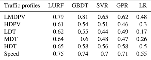
Table 1 illustrates the Pearson r used to evaluate the model performance with respect to predicting the daily averaged traffic parameters based on the constructed machine learning models. The overall predictive performance (Pearson's r, RMSE, and MAPE) is summarized in Table S5. Model performance was assessed using a 10-fold cross-validation. First, the LURF models consistently derive higher correlation coefficients between the predicted and observed traffic profiles than almost all of the other models. The Pearson r values range from 0.62 (LDTs) to 0.79 (LMDPVs) for the LURF models, which are higher than the corresponding correlation coefficients for the other four models. The r values of GBDT for LMDPVs are slightly better than those using LURF (0.81 vs. 0.79). Furthermore, the RMSE values of the category-resolved traffic volume values using the LURF models are significantly lower than those for the other models. The RMSE values of GBDT and SVR for HDT traffic simulations are also relatively low. With respect to the MAPE value, the performance of LURF, GBDT, and SVR is comparable and is better than that for GPR and LR. In general, LURF shows the best performance in the simulation of all traffic profiles, while the performance of GBDT and SVR for individual indicators (such as traffic flow of LMDPVs and HDTs) is also acceptable. Therefore, the LURF model is more capable of predicting traffic profiles than other models on most occasions in this study and will be used in the following simulations.

Table 1 The cross-validated mean Pearson r values of the traffic prediction by selected machine learning models.

We further developed a specific LURF model for each hour to predict the hourly averaged traffic profiles under different scenarios. We ranked the variable importance in the training process, utilizing the method above to construct a variable importance measure, and then averaged the hourly ranks for each variable to the final importance index listed in Table S6. Table S6 illustrates the top 10 most important variables for all land-use predictors in our LURF models under S1. In general, in addition to the road location (province, city, and county), the most important input variables for predicting traffic volume are primarily related to road information, such as the road type, road density, number of lanes, and designated speed. Especially for HDTs and speed simulations, the top 10 most important variables are almost all related to road information. The effects of land cover and POI information on estimating traffic characteristics are relatively less important than the role of road information. For passenger fleets (LMDPVs and HDPVs) and light-duty and medium-duty trucks (LDTs and MDTs, respectively), some important inputs related to the land-use datasets (e.g., population and POI information) are indicated by the analysis. Notably, these important land-use variables often represent large buffers (e.g., 2000 to 5000 m). This effect is because intercity monitoring sites are typically located far away from urban areas, where POI information is more densely available.

3.2 Traffic activity characteristics of road networks under various scenarios

In contrast to urban weekday–weekend patterns (Yang et al., 2019a), higher traffic activity is estimated on weekends (S2; 931 million vehicle kilometers) than on weekdays (S1; 841 million vehicle kilometers). This implies that more leisure trips on weekends could be captured by intercity highway monitoring data (see Fig. S5). The lower traffic activity on weekdays is mainly observed in Hebei Province (63 %); among all vehicle categories, LDPVs account for ∼70 % of the total reduced VKT, followed by HDTs (16 %) and LDTs (10 %).

We annualized the allocation of the total traffic activity by vehicle category in the BTH region by aggregating the daily patterns under S1 and S2 (see Fig. S6). Among all of the fleets, LDPVs account for the largest proportion of the total annual traffic activity (64 %), followed by HDTs (18 %) and LDTs (9 %). For HDTs, the fractions of the total traffic activity decrease from Hebei (20 %) to Tianjin (18 %) and, thus, to Beijing (11 %). This is likely due to two major reasons: (1) the passenger traffic activity of LDPVs is denser in Beijing than in Hebei and (2) many HDTs are restricted within the Sixth Ring Road in Beijing, which could also decrease the freight activity outside of the restricted area (Yang et al., 2019a). Table S7 illustrates the allocation of traffic activity by vehicle category and road type. For freight transportation, more than 50 % of HDT traffic activity is estimated to occur on expressways. In Tianjin and Hebei, HDTs more frequently travel on expressways than LDTs, in order to improve efficiency.

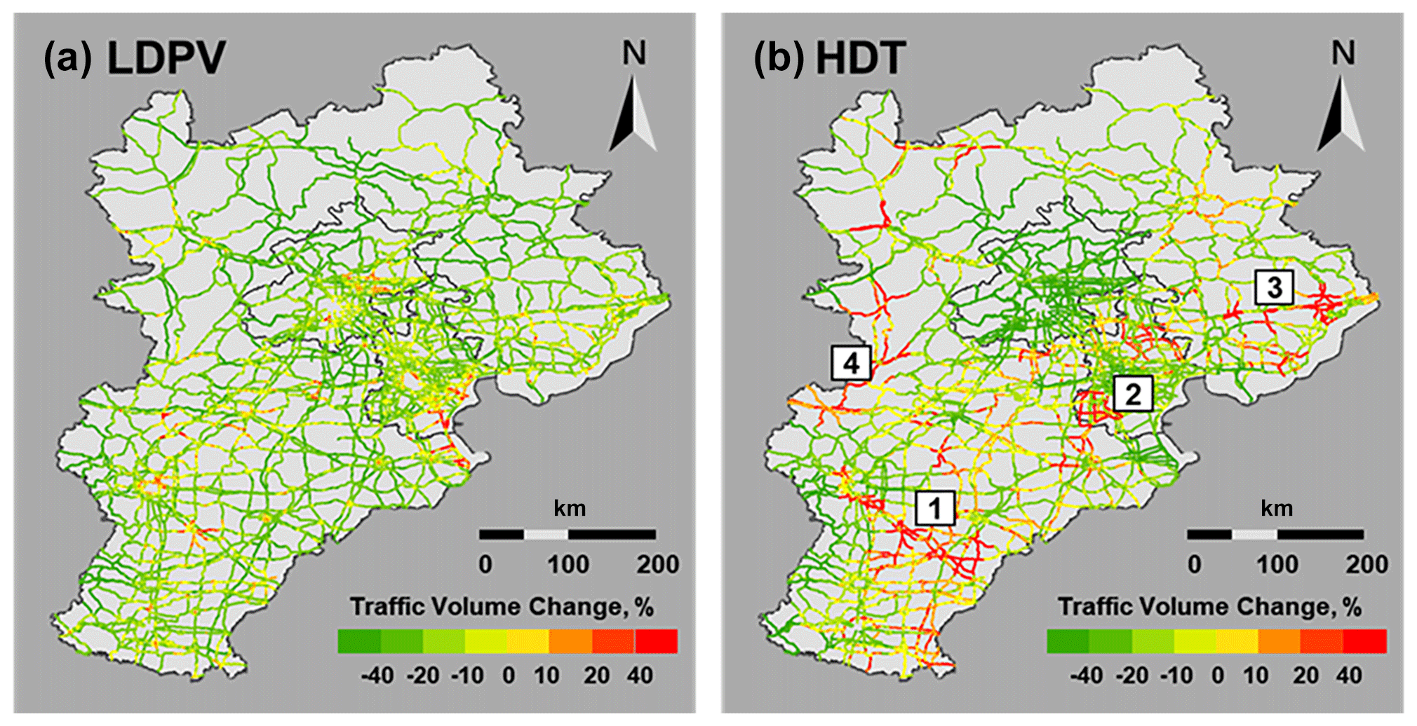
Figure 1 Estimated traffic volume reductions of LDPVs and HDTs under restricted traffic conditions (S3) compared with normal weekdays (S1).

In terms of temporal variations, the rush hour phenomenon, shown as an increase in the traffic activity, occurred from 08:00 to 10:00 GMT + 8 and from 15:00 to 17:00 GMT + 8 on weekdays (S1). Compared with the rush hour effect within urban areas in Beijing (e.g., which peaks at 07:00 GMT + 8) (Yang et al., 2019a), the morning rush hours occur later for these intercity highways, whereas evening rush hours are earlier. Similar trends are observed on weekends (S2), with higher traffic activity reflecting more casual intercity trips (see Fig. S5). In contrast, the diurnal fluctuations in the average speeds depict quite similar characteristics between weekdays and weekends (see Fig. S7) because the level of congestion for intercity highways (even during rush hours) is not comparable to urban areas. It should be noted that the speed in Beijing is obviously lower than that in Tianjin and Hebei, mainly due to the congestion that occurs in Beijing as a result of its larger travel demands.

The traffic activity in S3, which included special policy interventions, was clearly reduced in the BTH region: the daily traffic activity was decreased by 23 % compared with that of normal weekdays. Traffic reductions were also heterogeneous among the various vehicle categories and different regions. As Fig. 1 shows, LDPVs display uniform reductions of approximately 25 % on all of the intercity highways in the BTH region; only 4 % of roads are identified as having increased LDPV volume. For HDTs, reduced traffic could also be observed in Beijing and on the expressways and national highways in Tianjin, but a certain number of provincial highways in Tianjin (∼20 %) as well as expressways (∼30 %), national highways (∼15 %), and provincial highways (∼20 %) in Hebei showed increased flow. Four subregions with significantly increased HDT volume (more than 50 %) are indicated in Fig. 1. Subregions 1–3 represent the roads heading to several large ports (the ports of Qingdao, Tianjin, and Qinhuangdao for subregions 1–3, respectively), and subregion 4 represents the areas near the boundary of the BTH region. These differences in traffic volume between LDPVs and HDTs indicate that the restrictions could uniformly reduce the travel demand across the region for passenger travel. In contrast, decreases in HDT traffic volume are expected in areas with the stricter enforcement of traffic restrictions (i.e., Beijing and the highways and national roads in Tianjin). The traffic restrictions were more effective in Beijing, resulting in a 29 % decrease among all vehicle fleets, especially for HDTs (a 52 % decrease) and MDTs (a 42 % decrease). In Hebei, such traffic restrictions could result in HDTs taking detours, as the operators and drivers of HDTs even conducted their business on restrictive days. The decrease in the total traffic activity in Hebei was primarily due to LMDPVs, and the traffic activities of MDTs and HDTs were only 5 % and 14 % lower than those on normal weekdays (S1).

3.3 Temporal and spatial characteristics of traffic emissions

The total daily emissions for the intercity highways in the BTH region are estimated to be 1443 t for CO, 152.3 t for THC, 1158 t for NO_x, 37.30 t for PM_2.5, and 18.73 t for BC on weekdays (S1; see Fig. 2 and provincial-level total emissions and emission intensity in Fig. S8). On weekends (S2), the total daily emissions are estimated to increase by approximately 10 % for all pollutants due to increased traffic activity. Comprehensive traffic restrictions under S3 triggered decreased vehicle emissions (e.g., 33 %–38 % for CO and THC, 23 % for NO_x, and 15 %–17 % for PM_2.5 and BC) over the entire domain relative to S1. For LDPVs traveling on the highways, greater reductions in CO and THC result from the lower traffic volume due to traffic restrictions, especially in Tianjin and Hebei. In these areas, the controls on vehicles are behind those in Beijing; therefore, restrictions on pre-China II gasoline cars could result in a larger reduction. Diesel trucks contribute significantly to the emission reductions of NO_x, PM_2.5, and BC, and their lower reduction percentages compared with CO and THC are related to smaller decreases in the HDT traffic volume in Tianjin and Hebei.

Figure 2 Estimated hourly emissions by vehicle category under S1.

The major temporal difference in the diurnal patterns between S1 and S2 lies in the higher emissions during the weekend rush hours. Thus, we refer to the weekday scenario (S1) to elucidate the temporal and spatial emission patterns (see Figs. 2 and 3). The emission peaks of CO and THC during the morning (09:00 to 10:00 GMT + 8) and evening (16:00 to 17:00 GMT + 8) rush hours, which are apparently associated with diurnal fluctuations in the passenger travel demand, are shown in Fig. S5. As Fig. 4a and b visualize, the CO emission intensity close to urban areas is significantly higher than that in outlying areas during both peak and off-peak periods. The highest hourly emissions of CO and THC, which are more associated with passenger traffic activity, were estimated during the morning rush hour (10:00 GMT + 8); these emissions were approximately 40 %–50 % higher than their 24 h averages. The emission allocations show high resemblance between CO and THC; specifically, LDPVs dominate the contributions, and the proportions in Beijing and Tianjin are higher than those in Hebei. This increase is because the Beijing and Tianjin metropolitan areas have a higher density with respect to the residential population (indicated by pop_5000m), business units (indicated by POI_office_5000m), and urban lands (indicated by urbanland_5000m) than Hebei; these variables have been identified as the most important variables for traffic activity predictions of LDPVs using LURF modeling (see Table S6).

Figure 3 Link-based emission intensity of CO (a, b) and NO_x (c, d) during a midnight hour (00:00 GMT + 8) and a rush hour (10:00 GMT + 8).

Diesel fleets are responsible for much greater shares of on-road NO_x, PM_2.5, and BC emissions than CO and THC emissions. Consequently, distinctive traffic behaviors of diesel fleets will result in disparate temporal and spatial emission patterns compared with those for CO and THC. First, we have observed that the total emissions of NO_x, PM_2.5, and BC during the night (00:00 to 04:00 GMT + 8; Fig. 2) are closer to the emissions during the daytime, but the nighttime–daytime differences in the emission patterns are less than those of CO and THC. This finding is because a considerable portion of long-haul freight trucks in China are operated by two drivers, who could work in shifts and also travel during nighttime. Second, the NO_x, PM_2.5, and BC emission contributions of HDTs in Tianjin and Hebei are approximately 10 % higher than those in Beijing. Additionally, the higher percentages of total NO_x, PM_2.5, and BC emissions from HDPVs (tourist and intercity coaches) in Beijing are higher than those in Tianjin and Hebei. The comparison results indicated higher passenger travel demand in Beijing due to its attraction of tourists and lower freight transportation activity due to truck restrictions.

The emission maps discern the Port of Tianjin, the largest port in northern China with an annual freight handling amount of 466×10⁶ t in 2018, as a significant hotspot. A large amount of HDTs flood into the port (i.e., subregion 2 in Fig. 1), leading to significantly higher emissions on adjacent highways throughout the day (Fig. 3c, d). The daily variation in the NO_x emission intensity in the port area is more obvious than that in Tianjin and the BTH region, with a peak period from 07:00 to 18:00 GMT + 8. The hourly average NO_x emission intensity of the Port of Tianjin is 1.87±0.42 kg km⁻¹ h⁻¹, which is 47 % and 123 % higher than the average levels of Tianjin and the BTH region, respectively (see Fig. S9).

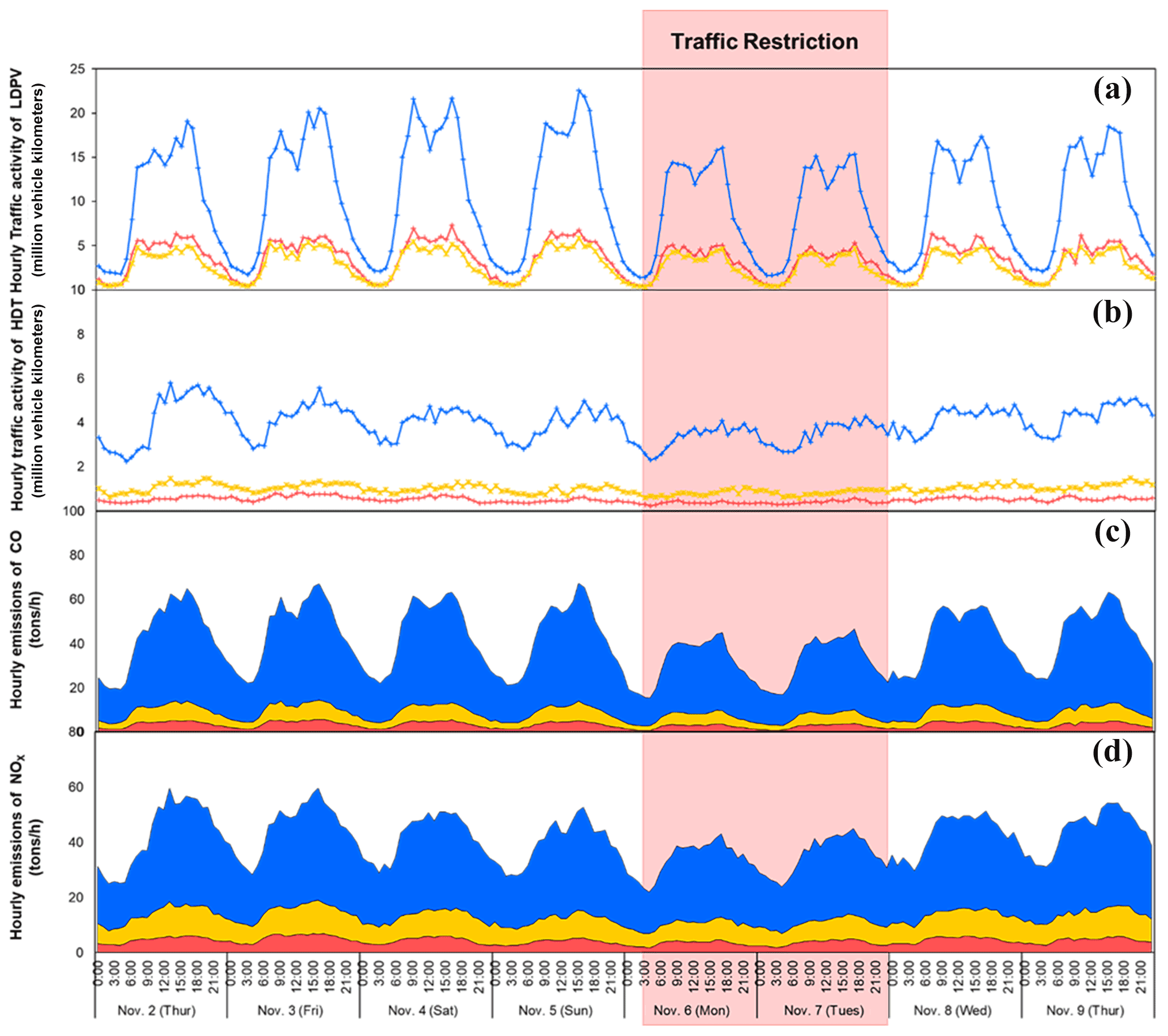
Figure 4 Hourly VKT for LDPVs and HDTs (a, b) as well as vehicle emissions of CO and BC (c, d) by region from 2 to 9 November 2017.

3.4 Discussion

3.4.1 An efficient protocol for dynamically modeling hourly based, link-level emissions

This study provides a universal analytical method for a high-resolution vehicle inventory at a regional scale, especially for regions including many cities that suffering from the difficulty of addressing traffic data at a high spatial resolution. Figure 4 shows the hourly variations in the traffic activities of LDPVs and HDTs as well as total vehicle emissions by region during a special week when traffic restrictions were implemented (specifically, on 5 and 6 November 2017). From 2 to 5 November, the traffic activity resembles that during a normal week (e.g., 20 to 27 April 2017; see Fig. S10). When traffic restrictions were implemented on 5 and 6 November, we observed a ∼20 % reduction in the VKT for LDPVs and HDTs, a ∼30 % reduction in CO emissions, and a ∼20 % reduction in NO_x emissions, which resembled S1 and S3 because of traffic restrictions. Therefore, the high efficiency of the calculation based on the LURF model provides a platform to realize the near-real-time process of establishing high-resolution vehicle emission inventories, and it can dynamically support the further evaluation of environmental benefits from traffic policies and management measures. However, the spatiotemporal dependencies are not as clearly modeled in machine learning as they are in general linear model frameworks, and future work could derive methods for optimizing the predictors used in machine learning models to improve the accuracy of the prediction.

3.4.2 Comparison of the best machine learning method against the standard empirical bottom-up approach

Addressing the spatial characteristics of traffic profiles based on limited datasets is a significant challenge for establishing high-resolution emission inventories of on-road vehicles. To overcome this barrier, the allocation of the VKT based on road information has been the most typical way of establishing simplified bottom-up inventories in previous studies. Zheng et al. (2014) allocated the VKT of each county based on the same weighting factors, considering the vehicle category and road type. Gately et al. used the same allocation of the total VKT, considering the differences in weighting factors according to the road type but without distinguishing the vehicle category. This section compared the differences between the abovementioned empirical methods and the machine learning method obtained in this study: M1 denotes the best machine learning method (i.e., LURF) in this study, and M2 denotes the allocation method based on the standard empirical bottom-up approach. The VKT of M2 was allocated based on a combination of the methods from Zheng and Gately (according to Eq. 2).

$$\begin{array}{}\text{(2)}& {\mathrm{VKT}}_{\mathrm{l},\mathrm{vc}}^{\mathrm{M}\mathrm{2}}={\mathrm{VKT}}_{\mathrm{vc}}^{\mathrm{M}\mathrm{1}}\times {\displaystyle \frac{{\mathrm{TV}}_{\mathrm{l},\mathrm{vc}}\cdot {\mathrm{RL}}_{\mathrm{l},\mathrm{vc}}}{{\sum }_{\mathrm{l}}{\mathrm{TV}}_{\mathrm{l},\mathrm{vc}}\cdot {\mathrm{RL}}_{\mathrm{l},\mathrm{vc}}}},\end{array}$$

where VKT${}_{\mathrm{vc}}^{\mathrm{M}\mathrm{1}}$ is the total VKT of vehicle category vc of the BTH region calculated in M1; VKT${}_{\mathrm{l},\mathrm{vc}}^{\mathrm{M}\mathrm{2}}$ is the allocated VKT on road link l of vehicle category vc in M2; TV_l, vc is the preallocated traffic volume based on its road type and location on road (Yang et al., 2019a) link l of vehicle category vc; and RL_l, vc is the length of road link l. CO and NO_x are discussed, as they represent emissions with gasoline and diesel features, respectively.

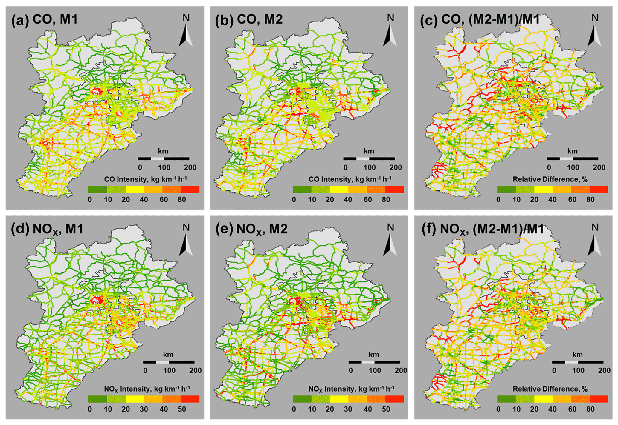
Figure 5 Comparison of the LURF method with the standard empirical bottom-up approach. M1 denotes the emission inventory based on the best machine learning method (LURF) in this study, and M2 denotes the emission inventory based on standard empirical bottom-up approach.

As Fig. 5 illustrates, compared with M1, M2 tends to underestimate the CO emissions on the provincial highways close to urban areas (80 % of the provincial highway links are underestimated) and overestimates the expressways and national highways in remote rural areas, especially in Beijing and Hebei (77 % and 62 % of the expressways are overestimated, respectively). This miscalculation is due to the fact that we tend to preallocate volume values according to the road rank for remote rural areas without monitoring traffic data; this means that expressways and national highways will be allocated a higher traffic volume than provincial roads. For NO_x, we observe a similar misestimation in the emission distribution of CO: approximately 70 % of provincial highway links are underestimated, and ∼70 % and 60 % of expressways and national highways are overestimated. The long-tailed distributions of the relative difference of CO and NO_x are illustrated in Fig. S11. Overall, the differences between the two methods are not extreme because 79 % and 82 % of the road links' respective relative differences for CO and NO_x are within ±50 %. The analysis indicates that we may use the simplified M2 without land-use data, although we would need to pay attention to the uncertainty in the project-level emission calculations (e.g., port-related areas).

Temporal and spatial patterns of air pollutant emissions from on-road vehicles are of substantial interest because of the associated potential public health impact. The population exposure to vehicular pollutants is greatest in areas with high vehicle usage and population density (Marshall et al., 2005). Air quality simulation models with fine-grained input from high-resolution vehicle emission inventories will be valuable for evaluating the potential health benefits from vehicle emission control measures (Ke et al., 2017). However, we are limited to estimates of detailed link-level emissions for urban areas in Tianjin and Hebei due to the data availability (e.g., traffic volume of urban local roads). Currently, as noted in Sect. 1, there are already link-level emission inventories in large cities with traffic datasets from the ITS (Intelligent Transportation System), but a strengthening of the portability of the analytical method is still needed. This study highlights a promising path to smart management of traffic emissions in various regions and cities by combining advanced data-driven techniques and multisource ITS datasets, which will provide policymakers with a better understanding of how air quality impacts regional and local transportation activities.

4 Conclusions

This paper developed an hourly link-level emissions inventory of vehicular pollutants using land-use machine learning methods based on the datasets of road traffic monitoring in the BTH region of China under three traffic scenarios. The methodology can potentially be used to map traffic characteristics on a larger scale or to deal with real-time urban traffic data streams that need to overcome the challenges of computational accuracy and efficiency. The major findings can be summarized as follows:

1. The land-use random forest (LURF) model is more capable of predicting traffic profiles than other models on most occasions in this research.

2. The most important input variables for predicting traffic volume values are primarily related to road information, such as the road type, road density, number of lanes, and designated speed.

3. Higher traffic activity is estimated on weekends than on weekdays, and the traffic activity of S3, which included special policy interventions, was reduced by 23 % compared with that of normal weekdays.

4. The model finds a general reduction in light-duty passenger vehicles when traffic restrictions were implemented but a much more spatially heterogeneous impact on heavy-duty trucks (HDTs).