the Creative Commons Attribution 4.0 License.
the Creative Commons Attribution 4.0 License.
 | 04 Feb 2022
Limitations of assuming internal mixing between different aerosol species: a case study with sulfate geoengineering simulations
Daniele Visioni
Simone Tilmes
Charles Bardeen
Michael Mills
Douglas G. MacMartin
Ben Kravitz
Jadwiga H. Richter
Simulating the complex aerosol microphysical processes in a comprehensive Earth system model can be very computationally intensive; therefore many models utilize a modal approach, where aerosol size distributions are represented by observation-derived lognormal functions, and internal mixing between different aerosol species within an aerosol mode is often assumed. This approach has been shown to yield satisfactory results across a large array of applications, but there may be cases where the simplification in this approach may produce some shortcomings. In this work we show specific conditions under which the current approximations used in some modal approaches might yield incorrect answers. Using results from the Community Earth System Model v1 (CESM1) Geoengineering Large Ensemble (GLENS) project, we analyze the effects in the troposphere of a continuous increasing load of sulfate aerosols in the stratosphere, with the aim of counteracting the surface warming produced by non-mitigated increasing greenhouse gas (GHG) concentrations between 2020–2100. We show that the simulated results pertaining to the evolution of sea salt and dust aerosols in the upper troposphere are not realistic due to internal mixing assumptions in the modal aerosol treatment, which in this case reduces the size, and thus the settling velocities, of those particles and ultimately changes their mixing ratio below the tropopause. The unnatural increase of these aerosol species affects, in turn, the simulation of upper tropospheric ice formation, resulting in an increase in ice clouds that is not due to any meaningful physical mechanisms. While we show that this does not significantly affect the overall results of the simulations, we point to some areas where results should be interpreted with care in modeling simulations using similar approximations: in particular, in the evolution of upper tropospheric clouds when large amounts of sulfate are present in the stratosphere, as after a large explosive volcanic eruption or in similar stratospheric aerosol injection cases. Finally, we suggest that this can be avoided if sulfate aerosols in the coarse mode, the predominant species in these situations, are treated separately from other aerosol species in the model.
- Article
(5941 KB) - Full-text XML
-
Supplement
(700 KB) - BibTeX
- EndNote


A comprehensive representation of aerosol processes in Earth system models is crucial for a variety of reasons. Aerosols are one of the main short-term forcing agents in the climate system, and uncertainties in the estimate of their overall forcing effects are still quite large (Boucher et al., 2013). Directly, they scatter incoming solar radiation, thus influencing surface temperatures, and they also absorb both solar radiation and outgoing planetary radiation, locally increasing air temperatures, modifying circulation patterns and affecting meteorology. Indirectly, they affect the climate by modifying cloud cover, acting as cloud condensation nuclei (CCN) and ice nuclei (IN), and changing clouds' physical and radiative properties (also through local atmospheric heating). Lastly, once they are deposited to the surface, they affect land and ice albedo through the melting of snow and ice. Aerosols at the surface also contribute to air pollution (especially via particulate matter (PM) below 2.5 and 10 µm in diameter, Ayala et al., 2012) and may affect soils and ecosystems through acid deposition (Vet et al., 2014).
Atmospheric aerosols may have different sizes, ranging from 0.001 to 100 µm in diameter, and their characteristics (number concentration, mass, shape, chemical composition and other physical properties) may change through emission (from natural or anthropogenic sources), nucleation (defined as the formation of new particles), coagulation (defined as the combination of existing aerosol particles, decreasing their number concentration but leaving the overall mass unaltered), condensational growth of chemical species in vapor form (such as H2SO4, NH3, HNO3 and volatile organics gases) on existing particles, gas-phase and aqueous-phase chemistry, water uptake (Ghan and Zaveri, 2007) and their removal through gravitational settling (dry deposition), in-cloud scavenging (defined as the removal of aerosol particles by precipitation particles) and below-cloud scavenging (defined as the capture of aerosol particles by precipitating droplets, Feng, 2009). They can, of course, be composed of different chemical species: the main components are usually sea salt, mineral dust, black carbon, organic matter, nitrate, ammonium and sulfate. Wang et al. (2020) provide a recent overview of all aerosol-related processes: this list of processes can give an idea of how challenging it can be to represent aerosol processes correctly in climate models, both due to the uncertainties in each process and in their combination, and because of the high computational burden necessary to correctly reproduce the known parts of each process. For this reason, most processes need to treat aerosols in parametrized ways with different complexities, ranging from the least (bulk model, considering all aerosols as described by a single mean radius and standard deviation) to the most complex (sectional model, considering a large number of “bins” of different sizes for each species where the aerosols can grow or shrink). An intermediate approach is the modal method: it works on the assumption that the actual size distribution of the aerosols can be represented by the combination of multiple lognormal functions with fixed standard deviations that are based on observations. Furthermore, a modal approach to aerosol microphysics must also make assumptions about the internal and external mixing of aerosol species (Fassi-Fihri et al., 1997): internal mixing is defined as the modeling of an aerosol particle as a mixing of the constituent species (Clarke et al., 2004), either as a homogeneous mix or as a coated sphere containing a solid core and coated by a liquid exterior. More simply put, it assumes that different species of aerosols in every grid box are present in the same proportion, and that their physical characteristics can be described by the same average size distribution. External mixing is defined as the treatment of particle populations as composed of different species with distinct compositions, and no assumption needs to be made with regards to the localized proportion of the various species, as they are treated differently (Riemer et al., 2019). Some discussion and comparisons of the application of sectional and modal microphysics modules in climate models can be found in Weisenstein et al. (2007), Kokkola et al. (2009), Kleinschmitt et al. (2017), and more specifically for sulfate geoengineering applications in Laakso et al. (2022).
A modal treatment of aerosols in climate models has been shown to successfully reproduce aerosol measurements for various events. In this work, in particular, we focus on the Community Atmosphere Model version 5.0 (CAM5) and its implementation in the Community Earth System Model (CESM), using the Modal Aerosol Module with three modes (MAM3, Liu et al., 2012). This approach has been shown to correctly reproduce tropospheric aerosols in a baseline climate (see Liu et al., 2012; Samset et al., 2014), and also to correctly reproduce the evolution of the stratospheric sulfate aerosol layer in the extreme case of explosive volcanic eruptions (Robock, 2000), as detailed by Mills et al. (2016, 2017) for the Whole Atmosphere Community Climate Model (WACCM) version of CESM1, with a high top (140 km) and 70 vertical layers. This model has been used for climate simulations of stratospheric aerosol intervention (SAI), a form of climate engineering that has been proposed (Budyko, 1969; Crutzen, 2006) as a way to temporarily reduce global surface temperatures by mimicking the cooling effect of volcanic eruptions through injecting SO2 in the stratosphere. In both the case of volcanic eruptions and for the proposed artificial injections, once SO2 reaches the stratosphere, it oxidizes, eventually forming gaseous H2SO4, which then either nucleates, forming new sulfate aerosol particles of H2SO4-H2O, or condenses onto existing particles (already existing particles could also coagulate, resulting in larger particles with the same overall mass). While this process transforms all SO2 into aerosols with an e-folding time of around 1 month (Mills et al., 2017), the produced aerosols tend to remain in the stratosphere for 1 year or more (Visioni et al., 2018b), and are removed through large-scale stratospheric circulation, which moves them poleward, or by gravitational settling or stratosphere–troposphere exchange, crossing the tropopause. Once in the troposphere, they are quickly removed through dry or wet deposition (Kremser et al., 2016).
Climate engineering simulations with CESM1(WACCM) in the Geoengineering Large Ensemble (GLENS; Tilmes et al., 2018a) have shown that it would be possible to maintain global surface temperatures at 2010–2029 levels even under a scenario where emissions of greenhouse gases (GHGs) continue unabated by increasing the amount of SO2 injected throughout the century. This technique may be able to reduce some of the harmful climatic effects produced by temperature increase (Tilmes et al., 2018a; Kravitz et al., 2019), by reducing the amount of incoming sunlight, but it would not be a perfect solution. In fact, the atmosphere and surface would be impacted in various ways by the produced aerosols, for example, the chemical composition of the stratosphere and the dynamical response produced by the local stratospheric heating (Richter et al., 2017; Tilmes et al., 2018b), which in turn can influence precipitation (Simpson et al., 2019) and the high-latitude seasonal cycle of temperature (Jiang et al., 2019). Once the aerosols are deposited to the surface they may also affect soils; however, considering the much larger amount of tropospheric sulfate aerosols produced by both natural and human activities, those settling from the stratosphere would have a marginal impact everywhere except in some pristine areas (Visioni et al., 2020b). Other processes that may be affected by SAI include aerosol interactions with cirrus clouds, which are a key component of the radiation balance. Water clouds at lower altitudes have a net cooling effect because they reflect solar radiation (see for instance Yi et al., 2017); on the other hand, the effect of cirrus clouds made of ice crystals and produced in the upper troposphere by supercooled water particles is harder to determine, but is widely understood to be positive (i.e., it produces a net warming at the surface; Fusina et al., 2007) due to their trapping of outgoing planetary radiation. Kuebbeler et al. (2012) and Visioni et al. (2018a) found in two different climate models (ECHAM-HAM5 and ULAQ-CCM, using a modal and a sectional aerosol approach, respectively) that the change in the vertical temperature gradient resulting from the stratospheric heating would reduce the formation of tropical cirrus ice clouds by less than 10 %, thus contributing to surface cooling. This effect is tied to the fact that, in both models, the amount of water vapor reaching the upper troposphere and which is necessary for cloud formation is directly tied to the available turbulent kinetic energy, which is a function of the vertical temperature gradient, and is therefore a purely dynamical effect. Cirisan et al. (2013) on the other hand investigated the possible microphysical effect of the increased sulfate load on cirrus cloud formation, but found no significant impact due to the much larger size of the aerosols from the stratosphere compared to those already present in the troposphere due to other activities.
In this study, as an example to illustrate some of the shortcomings of the modal aerosol treatment in MAM3, we use the GLENS simulations to explore the effects of a large amount of sulfate aerosols in the stratosphere on tropospheric aerosol concentrations and on cirrus ice cloud formation in CESM1(WACCM). We will briefly describe how aerosol microphysics and cirrus ice formation are parameterized in Sect. 2, then discuss how aerosols in the upper troposphere change in the simulations of interest in Sect. 3 and discuss how that affects upper tropospheric ice in Sect. 4. Finally, possible radiative effects at the top of the atmosphere of the identified changes will be discussed in Sect. 5.
In this section we will briefly describe the simulations used in this work, and then describe the components of the model that will be of use in our analysis.
The Geoengineering Large Ensemble (GLENS, Tilmes et al., 2018a) is an ensemble of simulations performed with CESM1 (WACCM), with all simulations using surface emissions from the Representative Concentration Pathway 8.5 (RCP) scenario. Twenty-one ensemble members are available for the period 2010–2030 under RCP8.5 (hereafter, termed Baseline). From each of these, in 2020 a scenario is simulated where SO2 is injected at four locations: 30∘ N and S, with injections at 23 km altitude, and 15∘ N and S at 25 km altitude. Each year, an algorithm (described by Kravitz et al., 2017) determines the amount of SO2 to be injected at each location in order to maintain the mean surface temperature, the inter-hemispheric surface temperature gradient, and the Equator-to-pole temperature gradient at their 2020 values in the presence of growing greenhouse gas concentrations. All the simulations of SAI are extended to 2100 (hereafter, termed GLENS), and four ensemble members of the Baseline cases (without SAI) are run to the at least the year 2097. Please note that, compared to the original simulations described in Tilmes et al. (2018a), one more ensemble member is available for both GLENS and Baseline (from 20 to 21 and from 3 to 4, respectively).
2.1 The Modal Aerosol Model in CESM
The Modal Aerosol Model (MAM) was first described by Liu et al. (2012), where it was evaluated for tropospheric aerosol loads. Some modifications have been made to include interactive stratospheric aerosols, described in depth by Mills et al. (2016), therein validated in the case of the Pinatubo 1991 eruption.
For CESM1(WACCM) climate simulations, the three-mode version (MAM3) is used, with aerosol species divided in three different lognormal modes of fixed width, named Aitken (dry diameter size range between 0.015 and 0.05 µm), accumulation (between 0.05 and 0.3 µm) and coarse mode (between 0.80 and 3.65 µm; all estimates from Liu et al., 2012), going from the smallest to the largest. Sulfate particles can grow by condensation (from H2SO4 vapor condensing on existing particles, locally maintaining particle numbers but increasing mass) or coagulation (locally reducing particle numbers but maintaining mass). When, by either process, the tail of the distribution of the particles in one of the modes grows to a size that would nominally be in the size range for the larger mode, the particles are transferred to the larger mode. This is done, as detailed by Easter et al. (2004), by defining a lower and upper limit for the dry diameter in each mode, and transferring part of the local number concentration to the larger mode when the threshold is surpassed. In the stratosphere the sulfate particles can also shrink due to evaporation, thus allowing for a coarse-to-accumulation mode transfer.
Compared to the more computationally demanding MAM version with seven aerosol modes (MAM7), in MAM3 all aerosol species are considered to be internally mixed within each of the three modes, thus sharing composition and size distribution. The mass for the single species has to be conserved, both globally and locally, and thus can only change in each grid box if particles are moved from one grid box to another, either because of air mass movement or because of gravitational settling or other tropospheric removal processes. Liu et al. (2012) justify this approach by noting that the sources of different aerosol types are geographically separated and thus unlikely to affect each other in the simplified version used for long-term climate applications. Coarse mode sulfate aerosols are, in quiescent conditions, also scarce in the troposphere: in the AeroCom multi-model mean (Textor et al., 2006) they were determined to be less than 2 % of all sulfate aerosols, with a preponderance of particles in the accumulation mode in the troposphere. The assumption by Liu et al. (2012) would therefore hold in the background atmosphere. We will show in the next section that the presence of the coarse mode sulfate particles produced by SAI fundamentally breaks this assumption, unnaturally modifying the size and quantity of non-sulfate aerosol species in the upper troposphere.
2.2 The formation of cirrus ice clouds in CESM
Cirrus clouds play an important part in the radiation budget, but have generally been poorly represented in general circulation models (GCMs) for a variety of reasons, among them a poor horizontal resolution which fails to capture the scale needed to represent some of the processes and a large spread in the ice water content simulated by models (Jiang et al., 2012). There are two processes that can produce ice crystals in the upper troposphere: homogeneous nucleation of ice crystals from sulfate aerosols and heterogeneous immersion freezing of mineral dust. Normally, homogeneous freezing is assumed to be the dominant process, although there are instances where this is not the case (Knopf and Koop, 2006; Cziczo et al., 2013). In the atmospheric model used in CESM1(WACCM), the Community Atmospheric Model version 5 (CAM5), both processes are present and we will briefly describe both below.
The process of homogeneous freezing is based on the assumption that only sulfate particles in the Aitken mode work as ice nuclei (IN), using the portion of the Aitken mode particles with radii greater than 0.1 µm (Liu and Penner, 2005; Liu et al., 2007). Other works have used all available sulfate modes for homogeneous freezing (Shi et al., 2015), and this would clearly affect the results. The process of homogeneous freezing is assumed to happen only when clouds are present, together with a probability distribution from Kärcher and Burkhardt (2008) that determines when the supersaturation is above the threshold for homogeneous freezing to happen. This means that homogeneous freezing can happen only when local vertical velocities are high (Kärcher and Lohmann, 2002). Those velocities are determined following Morrison and Pinto (2005) as
with the turbulent kinetic energy (TKE) determined using a steady state energy balance as in Bretherton and Park (2009).
For heterogeneous freezing, only coarse mode dust particles are assumed to be available IN (although the exclusion of soot particles and other particles as inefficient ice nuclei has been debated; see Kärcher and Burkhardt, 2008). Given the internal mixing assumption in MAM3, the number of available dust nuclei is determined as a fraction of the overall amount of coarse mode particles given the mass of dust and the overall aerosol mass
where md is the mass of dust in the coarse mode, mss is the mass of sea salt in the coarse mode and Nc is the total number of particles in the coarse mode. This approach assumes a negligible amount of coarse mode sulfate in the upper tropical stratosphere in the denominator of the fraction. Another shortcoming of the heterogeneous freezing description in this version of WACCM, as already discussed by Mills et al. (2017), is that when heterogeneous freezing occurs, IN that have nucleated to form ice particles are not removed from the available reservoir, thus allowing too many particles to be formed via heterogeneous freezing.
This approach to the microphysical modeling of cirrus clouds in CESM has been discussed recently by Maloney et al. (2019), who compared it with a more complex approach using the coupled Community Aerosol and Radiation Model for Atmospheres (CARMA) sectional scheme, and compared both with measurements from the National Aeronautics and Space Administration Airborne Tropical Tropopause Experiment (ATTREX 3) and with observations from the Cloud‐Aerosol Lidar with Orthogonal Polarization (CALIOP) onboard the CALIPSO satellite. They found that while the CAM5 approach was capable of correctly representing the annual average cloud fraction profile in the tropics (20∘ N to 20∘ S), it tended to underrepresent the cirrus fraction in the tropical tropopause layer. Similar results were also previously found by Bardeen et al. (2013).
The geographical distribution of tropospheric aerosols in the unperturbed atmosphere depends mainly on the surface sources of the aerosols or aerosol precursors; once the aerosols are produced in the atmosphere or are directly emitted, they can be affected by long range transport, upward currents and sediment through gravitational settling or scavenging. An in-depth analysis of sources and sinks of atmospheric aerosols can be found, for instance, in Lamarque et al. (2010). We focus here on sulfate, dust and sea salt, as their changes will be of interest when analyzing the effects on cirrus formation. Sulfate particles are mostly formed through surface emission of SO2, which can be oxidized to form sulfuric acid and then sulfate particles by condensation in the smaller (Aitken) mode. For this reason, coarse mode sulfate particles near the surface are much less frequent than dust or sea salt, as shown in Fig. 1a as compared to Fig. 1e and i. For the latter two, their concentration decreases with increasing altitude as the scavenging processes reduce their number, whereas there is an additional sulfate layer in the stratosphere (the Junge layer), discovered and discussed by Junge et al. (1961). This happens because of the presence of various sources of sulfate aerosols in the stratosphere, even without considering volcanic aerosols from explosive volcanic eruptions. In particular, surface emissions of carbonyl sulfide (OCS) and dimethyl sulfide (DMS), which are light, well-mixed gases that may reach the stratosphere where they are oxidized, forming sulfate aerosols (Vet et al., 2014). Meteoric sulfur also plays a part in the formation of the layer (see Gómez Martín et al., 2017). The quantity of sulfate aerosols produced in the stratosphere with an artificial injection of SO2 would be larger by some orders of magnitude than the amount in the quiescent Junge layer. The full stratospheric distribution in the case of GLENS has been described elsewhere (i.e., Kravitz et al., 2019), so here we simply report that at 50 hPa, between 30∘ N and 30∘ S, the average mass concentration for the last 20 years of simulation is 163 µg kg−1, compared to 0.4 µg kg−1 in the unperturbed case; while this simulation considered high cooling (∼4 ∘C reduction in global mean temperature), even much smaller amounts of SAI would lead to substantially more stratospheric sulfate than the unperturbed case. This magnitude is driven by the long lifetime of the produced aerosol particles in the stratosphere (around 12 months, Visioni et al., 2018b). Once the particles cross the tropopause, the various removal processes strongly reduce the lifetime, driving the concentration down. This is visible already in Fig. 1a, with the tropopause clearly visible as a change in concentration. Nonetheless, the average concentration of sulfate under SAI is much larger even in the upper troposphere (Fig. 1b) and only returns close to the Baseline levels close to the surface, where other sulfate sources are predominant (Fig. 1c).
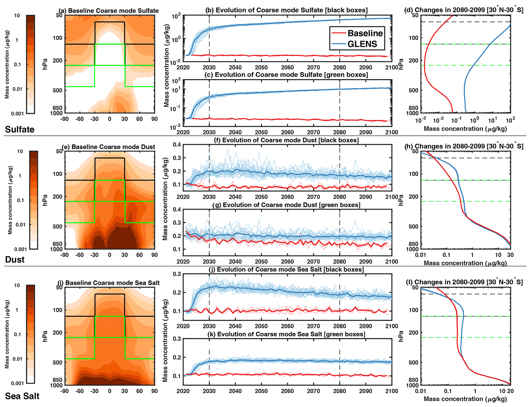
Figure 1Mass concentration (in micrograms per kilogram of air) of coarse mode species (sulfate, top row; dust, middle row; and sea salt, bottom row). On the left, panels (a), (e) and (i) indicate the Baseline (2020–2029) zonal mean concentration for the respective species, with the black and green boxes indicating the areas considered in the averages for the central panels (b, c, f, g, i, k). The uppermost limit of the green boxes and the lowermost limit of the black boxes coincide. Panels (b), (f), (j) and (c), (g) and (k) for each species show the annual evolution of the concentration in the black (b, f, j) and green (c, g, k) boxes, with thinner lines showing the single ensemble realizations, and the thicker lines show the ensemble mean; red lines indicate the Baseline simulations, while blue lines indicate the GLENS simulations. Black dashed lines in panels (b), (f), (j) and (c), (g) and (k) indicate the periods of analysis for panels (a), (e), (i) and (d), (h) and (l), respectively. On the right, panels (d), (h) and (l) show the vertical profiles in both cases (Baseline in red, and GLENS in blue) for the period 2080–2099. The black lines in panels (d), (h) and (l) indicate the altitude of analysis in panels (b), (f) and (j), while the green lines indicate the altitude of analysis in panels (c), (g) and (k).
Figure 1 also shows the behavior of dust and sea salt in the coarse mode in the same altitude–latitude region (those are the only other aerosol species considered in this version of CESM1 in the coarse mode: black carbon is only found in the accumulation mode). Various behaviors can be found depending on the altitude of analysis for the GLENS case. We focus here on the uppermost troposphere, right below the tropopause (black boxes in Fig. 1), and on a layer below, in the upper troposphere (green boxes). In the upper level, both dust (Fig. 1f) and sea salt (Fig. 1j) present behavior that is much more similar to that of sulfate: a large, initial increase in concentration in the first 5 to 10 years followed by either a constant evolution or by a small decrease (from 0.1 to 0.2 µm kg−1 for dust in the upper layer; from 0.06 to 0.2 µm kg−1 and from 0.9 to 0.17 µm kg−1 for sea salt in the upper and lower layer). Only dust in the lower layer (Fig. 1g) does not show such an abrupt initial increase. On the other hand, in the Baseline case, the dust mixing ratios show a decrease by 25 % over the 80 years of analysis in the lower level. There is no immediate physical mechanism by which such changes could be observed in aerosol species independent of sulfate; therefore, a more in-depth analysis is necessary.

Figure 2Zonally averaged total column burden of dust (a) and sea salt (c) (considering all modes) in 2010–2029 (red dashed line), 2080–2099 in Baseline (red line) and 2080–2099 in GLENS (blue line). Evolution of the globally integrated dust (b) and sea salt (d) burden (Tg yr−1). Thinner lines show the single ensemble realizations, while the thicker lines show the ensemble mean.

Figure 3Mass concentration (in micrograms per kilogram of air) of sulfate, dust and sea salt in the Aitken (smallest) mode and accumulation (intermediate) mode, between 30∘ N and 30∘ S. Thinner lines show the single ensemble realizations, while the thicker lines show the ensemble mean.
One possible explanation would be a change in the surface emissions of these species. However, the vertical profiles of tropical concentrations for the three species seem to exclude this (Figs. 1d, h, l and 3). This is further confirmed by the analysis of the overall burdens shown in Fig. 2. For these, no initial abrupt change can be identified, and the time evolution shows the opposite behavior from that found in Fig. 1, with a minor reduction in GLENS compared to Baseline. The behavior of the Baseline case is consistent with previous projections: Mahowald and Luo (2003) predicted a reduction in overall dust emissions with increasing GHGs due to higher precipitation and more surface moisture produced by the warmer air; thus the precipitation decrease in GLENS (Cheng et al., 2019) would exacerbate differences between dust burden in GLENS and the Baseline. Struthers et al. (2013) on the other hand projected a small increase in sea salt aerosols mostly as a result of increased surface wind speeds. Having excluded that changes in surface emissions are the cause of the abrupt increase identified, we further investigate the smaller aerosol modes (Fig. 3). In this case, we see a much closer agreement of the values in GLENS to those of the initial Baseline conditions for sea salt and dust: this indicates that the initial aim of the GLENS simulations, which was to maintain the state of the climate as close as possible to 2010–2029 conditions, also helps with not modifying surface emission sources of those species. The time evolution of the globally averaged quantities for these species and modes also does not show the same abrupt change as that found in Fig. 1 (see Figs. S1 and S2 in the Supplement). So, clearly the cause of the rapid change in concentration of the coarse mode must be the result of the very rapid increase in SO4 aerosol concentration, by more than 4 orders of magnitude.
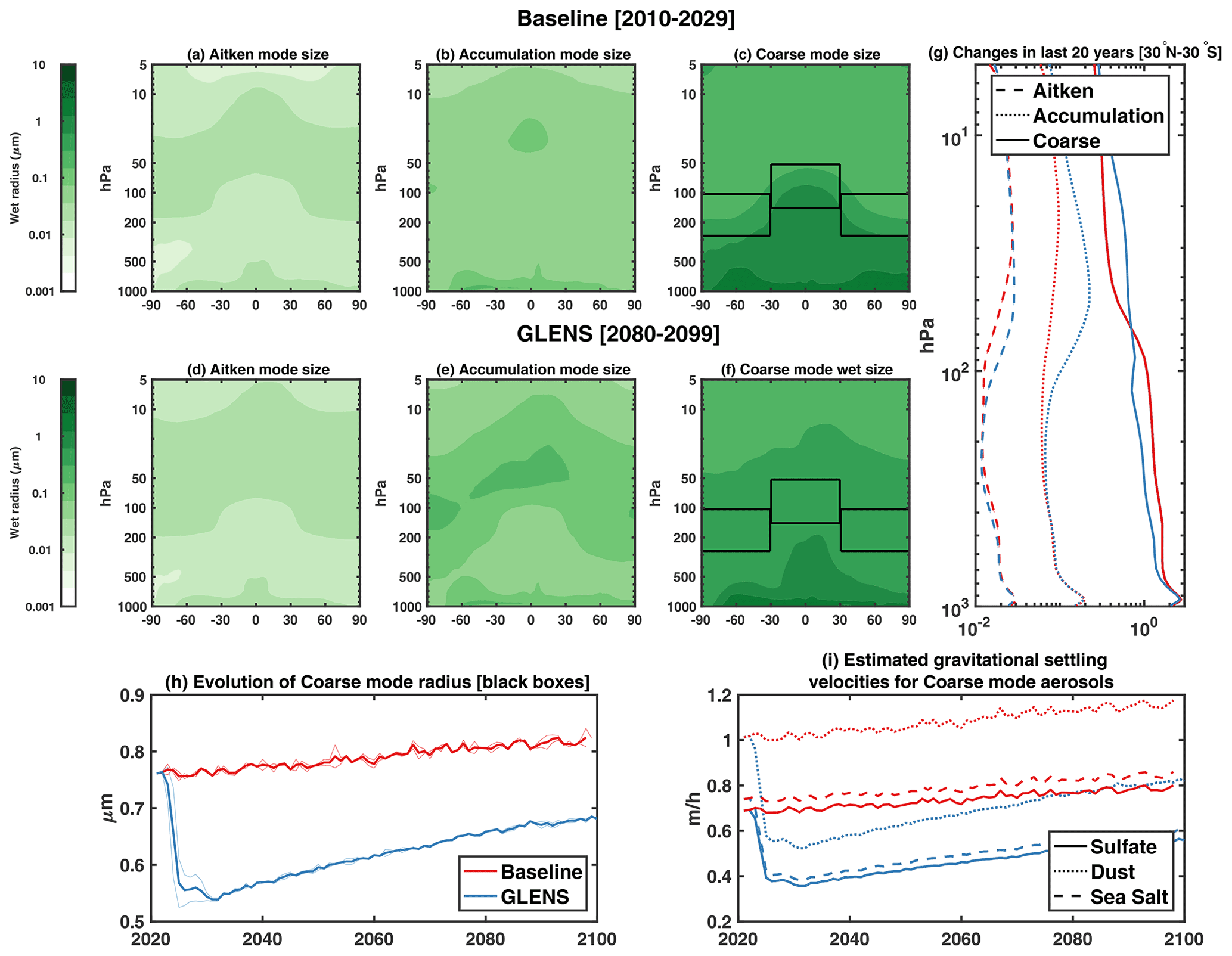
Figure 4Wet radius (in microns) of all three modes in the Baseline case ([2010–2029], a–d) and in GLENS ([2080–2099], e–h). (g) Vertical distribution of aerosol size in all three modes between 30∘ N and 30∘ S. Black boxes in panels (c)–(f) indicate the average area analyzed for panel (h), where the temporal evolution in Baseline (red) and GLENS (blue) is shown. Thinner lines show the single ensemble realizations, while the thicker lines show the ensemble mean. (i) Estimate of the changes in gravitational settling velocities following Seinfeld and Pandis (2016).
The solution to this conundrum can be found by analyzing the behavior of the simulated radius of the particles in the three modes (Fig. 4). In MAM3, all aerosol species within an aerosol mode are assumed to be internally mixed. The simplified assumption that different aerosols peak at different locations in the lower atmosphere is reasonable for the Baseline (Fig. 1 for the vertical distribution, and Fig. 2 for the spatial distribution). The parameterization requires that in each grid box, all aerosols in one mode are treated as the same in terms of their size distribution, so for each mode, only one mode diameter and one number concentration are used in the online calculations (since the geometric standard deviation is constant throughout the atmosphere). The mass concentrations of the different species are then calculated using a reference density for each species (Liu et al., 2012). This information is necessary to calculate the gravitational settling velocities (at each layer), which follow Seinfeld and Pandis (2016), where the equation of a free-falling spherical particle in a fluid that has reached terminal velocity (which is done in less than 1 × 10⁻⁶ for particles of diameter of ≃ 1 µm) is shown to be
where Dp is the diameter of the particle, ρp is the density of the particle, Cc is the slip-correction factor that accounts for non-continuum effects (dependent on the diameter of the particles) and CD is the empirical drag coefficient (dependent on the Reynolds number Re).
The initially identified changes can thus be explained as follows. The SO4 formed in the stratosphere is the predominant form of aerosols in the stratosphere, determining the radius of the particles at those altitudes. Most of these particles are in the coarse mode and therefore change the radius considered by the model in those grid boxes. Once the sulfate aerosols cross the tropopause (whether by gravitational settling, mostly in the tropics, or by large-scale circulation, at higher latitudes) they are added to the particle distribution already present in the upper troposphere. Due to the small amount of coarse mode aerosols there, and due to the internal mixing assumption in MAM3, the dust and sea salt aerosols already present are “forced” to reduce in size (and to conserve mass and to increase in number concentration; see Fig. S3). This produces a drop in the overall size by around 25 % within 3 years in the upper troposphere. Because of the strong dependence of gravitational settling velocities on size, the result is a drop in these velocities that, for dust aerosols, can be estimated to be over 40 %. This is not a direct output of the model, but we estimate it from Eq. (3) using the approach of Seinfeld and Pandis (2016). The clear drop in vt can then explain the initial identification of the increase in non-sulfate aerosol species: reducing settling deposition abruptly directly affects the concentration by decreasing removal, especially in regions where contributions from below are scarce. And the reason why this is only visible in the upper troposphere is that, further below, the preponderance of pre-existing, background coarse mode aerosol reduces the strength of this effect, not changing the radii. The preponderance of other removal mechanisms (in-cloud scavenging) also reduces the effect of the gravitational settling changes.
We have shown that the simulated changes in dust and sea salt in the upper troposphere in GLENS using CESM1(WACCM) are non-physical in nature. However, by looking at the concentration of the same species in the Baseline conditions it is clear that the overall presence of these aerosols at the altitudes of analysis is small, and therefore would have a negligible effect both when looking at the direct effects (for instance, on the radiative fluxes, which would be overshadowed by the effects of the sulfate aerosols in the stratosphere) and when eventually looking at surface effects. We show in this section, however, that their change does influence the simulation of ice cloud formation in the upper troposphere. Visioni et al. (2021) showed that some noticeable changes in cloud cover are present in the GLENS simulations, and that when separating the contribution of different types of clouds, most of these changes were attributable to changes in high clouds, which are defined in CESM1(WACCM) as all clouds formed between altitudes of 400 and 50 hPa. Furthermore, these changes were not as noticeable in other simulations performed where the same cooling as GLENS was achieved using a solar constant reduction approach, or where the stratospheric heating produced by the aerosols was imposed without the presence of the aerosol themselves. This points towards a contribution to the changes in high cloud cover in GLENS by some effects connected to the aerosol themselves. In particular, this points to changes in the freezing processes that produce ice crystals in the upper troposphere, given that at those altitudes there is much less water than in the lower troposphere, and most of it is in the form of ice rather than liquid droplets (see Fig. S5).
As we detailed in Sect. 2.2, there are two types of processes that may lead to the formation of ice crystals at those altitudes: the spontaneous freezing of small aqueous sulfate droplets at high relative humidity rates (Chen et al., 2000), known as homogeneous freezing, and the freezing of water droplets mediated by the presence of insoluble aerosol particles (ice nuclei, IN), known as heterogeneous nucleation (Diehl and Wurzler, 2004), which can happen at lower relative humidity conditions and higher temperatures (Knopf and Koop, 2006). Due to the difficulties in measuring the amount of ice crystals in the upper troposphere, and due to the challenges of representing the processes in models, there are plenty of uncertainties over the predominance of one formation process over the other. In CESM, only sulfate particles in the Aitken mode can act as the substrate over which homogeneous freezing can take place; this is generally understood to be correct, as too large particles would be increasingly harder to freeze (Chen et al., 2000). Since Aitken mode particles do not change in GLENS (see Fig. 3a), related changes in homogeneous freezing can be excluded, as already predicted by Cirisan et al. (2013). However, changes in homogeneous freezing may happen as a result of dynamical changes in the local vertical velocities that determine the amount of water vapor in the upper troposphere. Since the processes that determine those local vertical velocities happen at a much smaller scale compared to the resolution of climate models, they are usually parameterized in climate models as a function of vertical stability (see Eq. 1). Both previous studies analyzing the response of ice clouds in a SAI scenario, Kuebbeler et al. (2012) and Visioni et al. (2018a), used climate models with a similar parameterization as CESM, and found a reduction in ice cloud coverage because the warming of the stratosphere, combined with a cooling of the surface, produced a reduction in vertical temperature gradients and thus in the turbulent kinetic energy used to determine the velocities. A similar process can then be expected in CESM. Lastly, there is no physical reason why SAI would change heterogeneous freezing in ice clouds. However, given what we identified in the previous section related to dust aerosols in the upper troposphere, an influence on freezing processes cannot be excluded.
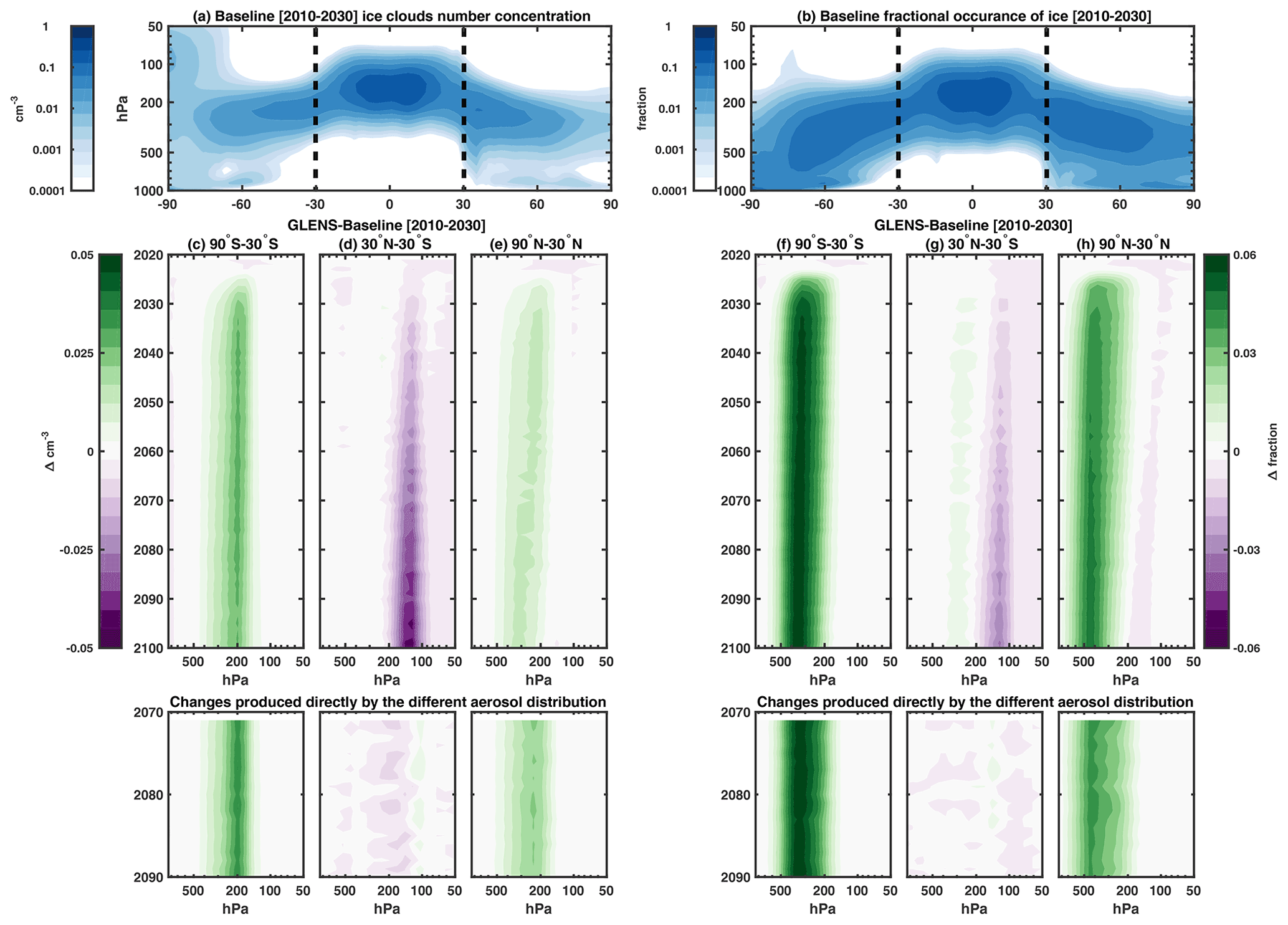
Figure 5Baseline concentration of cloud ice number concentration (a, number of particles per cm−3) and fractional occurrence (b) for the period 2010–2030. In panels (c)–(e) and (f)–(h), the yearly evolution of the differences between GLENS and Baseline (in the 2010–2030 period, as for the panels above) are shown for the three latitudinal boxes separately. In the small bottom panels, the effects of the changes produced by the aerosols are isolated by plotting the difference between GLENS and the simulations with surface cooling and stratospheric heating but no aerosols.
In Fig. 5, we show an analysis of the changes in the amount of ice in clouds under GLENS. Two particularly different behaviors can be noted when separating the effects at low latitudes (30∘ N–30∘ S) versus the effects noted elsewhere. At low latitudes, the dynamical changes produced by the different vertical stabilities dominate, resulting in a slow decrease in ice concentration in line with predictions discussed by Kuebbeler et al. (2012) and Visioni et al. (2018a), which is not a surprise, considering the very similar parameterization of sub-grid vertical velocities. At higher latitudes, where there are fewer changes in the vertical temperature gradient (since the stratosphere warms much less; see Richter et al., 2017), the predominant effect is the sudden increase in IN, resulting from the simplified aerosol treatment in the coarse mode. The increase in ice formation that the model “sees” is therefore not physical in origin, but simply an artifact of the microphysical parameterization and thus should not be treated as a physical side effect of SAI. A clue as to the two different mechanisms at play can be determined by observing the rate of change at low versus high latitudes. At low latitudes, the changes happen gradually as the stratospheric sulfate load (and thus the warming) increases. At high altitudes, the in-cloud ice changes are very abrupt, much more similar to the aerosol changes identified previously in this work. Further confirmation can be derived by observing the differences between the full GLENS simulations and the simulations described by Visioni et al. (2021) with stratospheric heating imposed, but no aerosols. By comparing the two (see bottom panels of Fig. 5), the effect of the presence of the aerosols can be separated from the dynamical ones, and indeed this confirms the different nature of the ice changes, since the two simulations (aerosols plus stratospheric heating and stratospheric heating alone) show no differences at low latitudes, whereas they are as different as GLENS-Baseline at high latitudes.

Figure 6Evolution of the occurrence of homogeneous freezing in clouds (a), the concentration of what the model considers to be IN for homogeneous freezing (Aitken mode sulfate) (b) and the concentration of IN for heterogeneous freezing (coarse mode dust) (c) in GLENS in the first 21 years of simulation, for the three latitudinal bands already considered in Fig. 5. On the right, a column mean of between 50 and 400 hPa is considered (thick lines), together with the case described in the text with a sensitivity test for Eq. (2) (dotted lines). In panel (f) the ice number concentration shown in Fig. 5 is compared with that of the sensitivity experiment.
Further information would be gained by observing the changes in heterogeneous versus homogeneous freezing in these simulations. However, the output fields that separate the two processes have not been saved in the original simulations from GLENS. Therefore, a complete analysis is not possible using the whole ensemble and time period. Noting that the main, unexplained processes (with our current understanding of ice formation) happen in the very first decade of the simulations, for the following analysis we have re-run the first 21 years of one of the ensemble members with the same configuration (thus, bit-by-bit, the result is the same) but retain information related to the two different upper tropospheric freezing processes. The results in Fig. 6 confirm our previous observations. For homogeneous freezing, very few changes are initially observable at any latitude, whereas large, abrupt changes are observable in the concentration of what the model considers to be IN for heterogeneous freezing in the first few years. This increase is much larger than the increase in the coarse mode dust aerosols identified in Fig. 1, where the overall concentration was doubled, while here the increase is much larger, at more than 10 times the amount in the first 2 years. To partially explain this change, we refer to the equation used by the model to determine the fraction of the available dust in the coarse mode, which is used as IN for heterogeneous freezing (Eq. 2). The available number of dust particles that can be used by the model depends on the overall amount of coarse mode particles, but it is weighted by the local fraction of aerosol comprised of dust to that comprised of sea salt. This formula (which in normal conditions gives satisfactory results; see Maloney et al., 2019) presumes a lack of sulfate in the upper troposphere. In our case however, as we have shown, the amount of coarse mode sulfate is actually by far preponderant in the upper troposphere. So while the number of coarse mode particles Nc grows (see Fig. S3), the fraction of all aerosols that is considered does not. This is a separate, but similar, problem as the one noted regarding the behavior of the aerosols. We tested how sensitive this assumption is by performing an identical simulation to the one that gave us information about homogeneous and heterogeneous freezing, but modified the code so that Eq. (2) becomes
thus correctly accounting for the mass of sulfate when considering the fraction of locally present coarse mode particles comprised of dust aerosols. We show the results of these sensitivity simulations in Fig. 6 using dotted lines: as expected, this does not change the homogeneous freezing processes, but it does change the amount of heterogeneous IN, and reduces the non-physical increase in cloud ice identified in Fig. 5 at high latitudes.
Here we investigate whether the changes shown in the previous section produce some signal in the modeled radiative fluxes at the top of the atmosphere, as that would be important in determining the effect's significance. To do so, we use the method suggested by Ghan (2013) to separate both the direct radiative effect of the aerosols and the effect of cloud changes produced by the aerosols. This is possible here as the radiative output of CESM is both comprised of the full radiative fluxes (FALL) at the top of the atmosphere (TOA), which consider all effects from aerosols, clouds and atmospheric composition, and comprised of the diagnosed Clear Sky radiative fluxes (where the radiative transfer model calculates the radiative fluxes as if no clouds were present, FCLEAR), Clean Sky radiative fluxes (where the radiative fluxes are calculated as if no aerosols were present, FCLEAN) and their combination (FCLEAN,CLEAR). This allows for the separation of the contributions of the added aerosols and their effects for both the longwave (LW) and shortwave (SW) components: the direct forcing produced by the aerosols direct interaction with the radiation (ΔFD) can be defined as
and the forcing produced by the changes in clouds (ΔC) can be defined as
As Ghan (2013) notes, normally these fluxes are just an estimation of the real components of the forcing, as to properly estimate them it would be necessary to keep the surface and tropospheric temperatures fixed between the two cases in order to avoid changes in the radiative emissions of the troposphere, which would be at different temperatures in the two cases. In our case, however, the GLENS simulations have been performed on purpose to maintain similar global surface temperatures as the Baseline 2010–2030 period; some small regional temperature differences are still present (Tilmes et al., 2018a), but overall these can be considered a minor factor and the estimated forcing can be considered to be quite robust if we always compare the radiative fluxes against the 2010–2030 period. In the case of cloud changes, this further ensures that we are not counting effects produced by the surface warming, which might also locally modify cloud cover.

Figure 7Global mean evolution of TOA radiative fluxes in the LW (orange), SW (green) and Net (black) for the forcing directly produced by the aerosols ΔFD (a) and by the clouds as changed by the presence of the aerosols (ΔC) (d). In panels (b)–(c) and (e)–(f), respectively, the latitudinal breakdown of the global fluxes in two periods (2026–2035 and 2081–2100) is shown for the various components. To the right of each panel, the global mean in the considered period is shown with a triangle of the same color, and the value is given on the right. Thinner lines show the single ensemble realizations, while the thicker lines show the ensemble mean.
In Fig. 7 we show the global evolution of ΔFD and ΔC in GLENS. The aerosol direct radiative effect is linear: negative in the shortwave (implying a cooling), as it reflects incoming sunlight, and positive in the longwave (implying a warming), as it absorbs and re-emits longwave radiation, with an overall negative effect, as expected. We show the latitudinal breakdown of the fluxes in Fig. 7b–c normalized by the stratospheric aerosol optical depth (AOD) produced by the SO2 injections for the initial period (we pick 2026–2035 to avoid the very first few years when the algorithm that determines the SO2 injections is still converging; see Kravitz et al., 2017) and the last 20 years (2081–2100). A partial non-linearity can be identified between the two periods. This can be explained by the slight increase in stratospheric sulfate aerosol during the whole period of analysis (see Visioni et al., 2020a; the effective radius in the stratosphere in GLENS grows from 0.4 to over 0.5 µm as a result of the increasing injection rates resulting in more coagulation of SO2 with pre-existing particles). Larger aerosols scatter slightly less efficiently, but they absorb more LW radiation. The changes in upper tropospheric aerosols described earlier do not influence these radiative fluxes, as they are, in proportion, negligible compared to the stratospheric increase. Looking at the ΔC fluxes, however, we can see that the behavior of the LW ΔC shows a very different behavior compared with the SW. This effect is positive in the first ≃ 30 years, and then negative afterwards, whereas the SW forcing is always positive. The SW forcing is easily explainable as directly connected to the presence of the aerosols above: if less sunlight reaches the troposphere, because it is partially reflected in the stratosphere, the same clouds would appear to be less reflective, and hence the positive sign of the SW (cloud masking). This does not apply to the LW, as globally the surface temperatures are the same, but can be explained by noting that the main contributor to LW trapping by clouds is upper tropospheric ice (Fusina et al., 2007). Since, in the first decades, mid-latitudinal ice clouds increase as shown in Fig. 5 because of “more” dust aerosols acting as IN, they would trap more outgoing LW radiation. When tropical ice clouds start decreasing because of the dynamical mechanism produced by stratospheric heating, the positive bump is erased by negative forcing (less ice clouds, more LW radiation escaping to space) already analyzed by Visioni et al. (2018a). This is further confirmed by the latitudinal breakdown of ΔC in Fig. 7e–f, where the (normalized by stratospheric AOD) forcing in the LW goes from positive in the first 10 years to negative in the last 20 years.
In this work we have identified the presence of some weaknesses in the three-mode modal approach (MAM3) used in CESM1(WACCM) when a large amount of aerosols settles down from the stratosphere, as under stratospheric sulfate aerosol injection, which results in some artificial changes to cirrus clouds. MAM3 only separates the species in three modes depending on their size, by treating all aerosol species as the same (internal mixing assumption). When a large amount of sulfate is produced (mostly in the coarse mode, the largest mode) in the stratosphere following the injection of SO2 in large quantities, the particles slowly descend upon the troposphere, where they are quickly removed. However, the size of the coarse mode particles is different (smaller) compared to that of the coarse mode particles already present in the troposphere, whose source is at the surface. Therefore, MAM3 “sees” an abrupt decrease in all aerosol sizes in each grid box in the upper troposphere for the coarse mode, resulting in smaller settling velocities for aerosol species that would not be otherwise affected in the real world. This effect results in an increase in the mass of particles of all species at those altitudes, even if there were no natural causes. The effect is small, and its direct effect on the cooling produced by the stratospheric aerosols is negligible. However, the unnatural addition of dust in the upper troposphere results in more particles that the model can use as solid ice nuclei for the freezing of ice particles in clouds. This effect is particularly evident at mid- and high latitudes, where the low relative humidity and lack of aerosols make other ice formation processes more scarce in normal conditions. The formation of these ice crystals, as simulated by the model, indeed produces a noticeable change in the cloud forcing, especially in the first years, when the effect from the incorrect presence of the dust aerosols is large compared to other, dynamical effects that tend to reduce the amount of ice crystals in the upper troposphere when a warming of the stratosphere is present.
Given the setup of the GLENS experiments, this effect is counteracted by the presence of the algorithm that determines how much SO2 is needed every year to counteract the effect of the increased emissions in RCP8.5: even if the radiative imbalance were to be large, the algorithm would just prescribe more SO2 to be injected, therefore resulting, overall, in the same global mean temperatures as if the error in the ice cloud formation was not there. In the sensitivity simulations produced for Sect. 4, which reduced the amount of ice clouds incorrectly formed by the model, the cumulative amount injected in the first 20 years was 131 Tg SO2 (6.2 Tg SO2 yr−1), whereas the same period in the default simulation had a cumulative amount of 154 Tg SO2 (7.3 Tg SO2 yr−1). Considering that, aside from the change in Eq. (2), the two simulations were otherwise the same; we can assume that this difference arises from the changes in ice clouds as simulated by the model. Overall then, if we assume this effect is constant throughout the whole simulation period, it would account for a cumulative injected 88 Tg SO2 over the entire century. While this amount might seem large, it accounts for less than 2 years of anthropogenic emissions of SO2 at present (Visioni et al., 2020b). This, furthermore, assumes a very large injection to overcome a considerable amount of warming (over 4∘) over the entire century. More moderate mitigation scenarios would require far less cumulative injections of SO2 (for instance, see Tilmes et al., 2020).
This does not imply that the effect can be ignored, but suggests that going forward when using a modal approach to aerosol microphysics, simulations where large amount of sulfate is present in the stratosphere should treat sulfate aerosols in a separate coarse mode that is not internally mixed with the other species compared (dust, sea salt, black carbon, etc.). A similar approach has already been used to include an additional primary carbon mode in MAM4 (Liu et al., 2016) in order to account for processes that affect the microphysical properties of primary carbonaceous aerosols in the atmosphere. There are various applications where this observation might be useful: SAI is one example, but the simulation of explosive volcanic eruptions is another case where it could be useful. For instance, Schmidt et al. (2018) used the same CESM1(WACCM) model described here to estimate the global volcanic radiative forcing in the last 45 years, and made a similar observation as that in this paper, but did not find an explanation. The mechanism that produced, in their simulations, an increase in ice particles in the upper troposphere is definitely the same we have encountered here, and would explain some of the LW forcing changes diagnosed in their simulations with a similar method (see Figs. 4 and 5 in Schmidt et al., 2018). More generally, it would be crucial to properly represent the upper troposphere in the case of volcanic eruptions to verify their influence on ice clouds as observed by some studies of the observational record (see for instance Friberg et al., 2015). Future modeling efforts aimed at better understanding the climatic effect of volcanic eruptions, such as the Volcanic Model Intercomparison Project (Clyne et al., 2021) or the Interactive Stratospheric Aerosol Model Intercomparison Project (Timmreck et al., 2018), should take this into account and consider how that might affect some of their results, since models with similar modal approaches are present in both.
Lastly, this observation would also be crucial in studies that aim to combine sulfate injections with the artificial seeding of upper tropospheric ice clouds with solid nuclei in order to increase the size of the ice crystal and make them sediment faster (cloud seeding, Gasparini et al., 2020). Cao et al. (2017), for instance, proposed a combination of the two methods to stabilize global temperatures and precipitation. Such simulations, performed with CESM1(WACCM) or any model with a similar microphysical approach, would not give meaningful results. Our study shows that more care should be given to make sure that the climate models used for simulating sulfate geoengineering applications are not applied outside of the parameters for which the models give reliable answers. Most of the time, models are also compared against volcanic events to make sure they properly simulate results, but not every effect is immediately visible in those cases as compared to long-term geoengineering simulations, and a comparison of cloud changes after a volcanic eruption may be complicated by various factors (Friberg et al., 2015).
All simulations analyzed in this work are available online. All GLENS simulations data are available at https://doi.org/10.5065/D6JH3JXX (Tilmes et al., 2018c). Data from the stratospheric heating simulations used for Fig. 5 are available at https://doi.org/10.7298/z8c9-3p43 (Visioni and MacMartin, 2021).
The supplement related to this article is available online at: https://doi.org/10.5194/acp-22-1739-2022-supplement.
DV performed the analysis and wrote the manuscript. ST, CB and MM contributed to the analysis and with the interpretation of MAM3 and ice formation processes results. DGM, BK and JHR offered helpful suggestions on the manuscript and analysis.
The contact author has declared that neither they nor their co-authors have any competing interests.
Publisher’s note: Copernicus Publications remains neutral with regard to jurisdictional claims in published maps and institutional affiliations.
This article is part of the special issue “Resolving uncertainties in solar geoengineering through multi-model and large-ensemble simulations (ACP/ESD inter-journal SI)”. It is not associated with a conference.
Ben Kravitz would like to acknowledge the Pacific Northwest National Laboratory, which is operated for the U.S. Department of Energy by the Battelle Memorial Institute under contract DE-AC05-76RL01830. The authors would like to acknowledge the CESM project, which is supported primarily by the National Science Foundation.
This research has been supported by the National Science Fundation (grant nos. CBET-1818759 and CBET-1931641) and by the Atkinson Center for a Sustainable Future at Cornell University.
This paper was edited by Fangqun Yu and reviewed by three anonymous referees.
Ayala, A., Brauer, M., Mauderly, J. L., and Samet, J. M.: Air pollutants and sources associated with health effects, Air Qual. Atmos. Hlth., 5, 151–167, 2012. a
Bardeen, C. G., Gettelman, A., Jensen, E. J., Heymsfield, A., Conley, A. J., Delanoë, J., Deng, M., and Toon, O. B.: Improved cirrus simulations in a general circulation model using CARMA sectional microphysics, J. Geophys. Res.-Atmos., 118, 11679–11697, https://doi.org/10.1002/2013JD020193, 2013. a
Boucher, O., Randall, D., Artaxo, P., Bretherton, C., Feingold, G., Forster, P., Kerminen, V.-M., Kondo, Y., Liao, H., Lohmann, U., Rasch, P., Satheesh, S., Sherwood, S., Stevens, B., and Zhang, X.: Climate Change 2013: The Physical Science Basis. Contribution of Working Group I to the Fifth Assessment Report of the Intergovernmental Panel on Climate Change, in: Fifth Assessment Report of the Intergovernmental Panel on Climate Change, IPCC, available at: https://www.ipcc.ch/site/assets/uploads/2018/02/WG1AR5_Chapter07_FINAL-1.pdf (last access: 12 January 2022), 2013. a
Bretherton, C. S. and Park, S.: A New Moist Turbulence Parameterization in the Community Atmosphere Model, J. Climate, 22, 3422–3448, https://doi.org/10.1175/2008JCLI2556.1, 2009. a
Budyko, M. I.: The effect of solar radiation variations on the climate of the Earth, Tellus, 21, 611–619, https://doi.org/10.1111/j.2153-3490.1969.tb00466.x, 1969. a
Cao, L., Duan, L., Bala, G., and Caldeira, K.: Simultaneous stabilization of global temperature and precipitation through cocktail geoengineering, Geophys. Res. Lett., 44, 7429–7437, https://doi.org/10.1002/2017GL074281, 2017. a
Chen, Y., DeMott, P. J., Kreidenweis, S. M., Rogers, D. C., and Sherman, D. E.: Ice Formation by Sulfate and Sulfuric Acid Aerosol Particles under Upper-Tropospheric Conditions, J. Atmos. Sci., 57, 3752–3766, https://doi.org/10.1175/1520-0469(2000)057<3752:IFBSAS>2.0.CO;2, 2000. a, b
Cheng, W., MacMartin, D. G., Dagon, K., Kravitz, B., Tilmes, S., Richter, J. H., Mills, M. J., and Simpson, I. R.: Soil Moisture and Other Hydrological Changes in a Stratospheric Aerosol Geoengineering Large Ensemble, J. Geophys. Res.-Atmos., 124, 12773–12793, https://doi.org/10.1029/2018JD030237, 2019. a
Cirisan, A., Spichtinger, P., Luo, B. P., Weisenstein, D. K., Wernli, H., Lohmann, U., and Peter, T.: Microphysical and radiative changes in cirrus clouds by geoengineering the stratosphere, J. Geophys. Res.-Atmos., 118, 4533–4548, https://doi.org/10.1002/jgrd.50388, 2013. a, b
Clarke, A. D., Shinozuka, Y., Kapustin, V. N., Howell, S., Huebert, B., Doherty, S., Anderson, T., Covert, D., Anderson, J., Hua, X., Moore II, K. G., McNaughton, C., Carmichael, G., and Weber, R.: Size distributions and mixtures of dust and black carbon aerosol in Asian outflow: Physiochemistry and optical properties, J. Geophys. Res.-Atmos., 109, D15S09, https://doi.org/10.1029/2003JD004378, 2004. a
Clyne, M., Lamarque, J.-F., Mills, M. J., Khodri, M., Ball, W., Bekki, S., Dhomse, S. S., Lebas, N., Mann, G., Marshall, L., Niemeier, U., Poulain, V., Robock, A., Rozanov, E., Schmidt, A., Stenke, A., Sukhodolov, T., Timmreck, C., Toohey, M., Tummon, F., Zanchettin, D., Zhu, Y., and Toon, O. B.: Model physics and chemistry causing intermodel disagreement within the VolMIP-Tambora Interactive Stratospheric Aerosol ensemble, Atmos. Chem. Phys., 21, 3317–3343, https://doi.org/10.5194/acp-21-3317-2021, 2021. a
Crutzen, P. J.: Albedo Enhancement by Stratospheric Sulfur Injections: A Contribution to Resolve a Policy Dilemma?, Climatic Change, 77, 211–220, https://doi.org/10.1007/s10584-006-9101-y, 2006. a
Cziczo, D. J., Froyd, K. D., Hoose, C., Jensen, E. J., Diao, M., Zondlo, M. A., Smith, J. B., Twohy, C. H., and Murphy, D. M.: Clarifying the Dominant Sources and Mechanisms of Cirrus Cloud Formation, Science, 340, 1320–1324, https://doi.org/10.1126/science.1234145, 2013. a
Diehl, K. and Wurzler, S.: Heterogeneous Drop Freezing in the Immersion Mode: Model Calculations Considering Soluble and Insoluble Particles in the Drops, J. Atmos. Sci., 61, 2063–2072, https://doi.org/10.1175/1520-0469(2004)061<2063:HDFITI>2.0.CO;2, 2004. a
Easter, R. C., Ghan, S. J., Zhang, Y., Saylor, R. D., Chapman, E. G., Laulainen, N. S., Abdul-Razzak, H., Leung, L. R., Bian, X., and Zaveri, R. A.: MIRAGE: Model description and evaluation of aerosols and trace gases, J. Geophys. Res.-Atmos., 109, D20210, https://doi.org/10.1029/2004JD004571, 2004. a
Fassi-Fihri, A., Suhre, K., and Rosset, R.: Internal and external mixing in atmospheric aerosols by coagulation: Impact on the optical and hygroscopic properties of the sulphate-soot system, Atmos. Environ., 31, 1393–1402, https://doi.org/10.1016/S1352-2310(96)00341-X, 1997. a
Feng, J.: A size-resolved model for below-cloud scavenging of aerosols by snowfall, J. Geophys. Res.-Atmos., 114, D08203, https://doi.org/10.1029/2008JD011012, 2009. a
Friberg, J., Martinsson, B. G., Sporre, M. K., Andersson, S. M., Brenninkmeijer, C. A. M., Hermann, M., van Velthoven, P. F. J., and Zahn, A.: Influence of volcanic eruptions on midlatitude upper tropospheric aerosol and consequences for cirrus clouds, Earth Space Sci., 2, 285–300, https://doi.org/10.1002/2015EA000110, 2015. a, b
Fusina, F., Spichtinger, P., and Lohmann, U.: Impact of ice supersaturated regions and thin cirrus on radiation in the midlatitudes, J. Geophys. Res.-Atmos., 112, D24S14, https://doi.org/10.1029/2007JD008449, 2007. a, b
Gasparini, B., McGraw, Z., Storelvmo, T., and Lohmann, U.: To what extent can cirrus cloud seeding counteract global warming?, Environ. Res. Lett., 15, 054002, https://doi.org/10.1088/1748-9326/ab71a3, 2020. a
Ghan, S. J.: Technical Note: Estimating aerosol effects on cloud radiative forcing, Atmos. Chem. Phys., 13, 9971–9974, https://doi.org/10.5194/acp-13-9971-2013, 2013. a, b
Ghan, S. J. and Zaveri, R. A.: Parameterization of optical properties for hydrated internally mixed aerosol, J. Geophys. Res.-Atmos., 112, D10201, https://doi.org/10.1029/2006JD007927, 2007. a
Gómez Martín, J. C., Brooke, J. S. A., Feng, W., Höpfner, M., Mills, M. J., and Plane, J. M. C.: Impacts of meteoric sulfur in the Earth's atmosphere, J. Geophys. Res.-Atmos., 122, 7678–7701, https://doi.org/10.1002/2017JD027218, 2017. a
Jiang, J., Cao, L., MacMartin, D. G., Simpson, I. R., Kravitz, B., Cheng, W., Visioni, D., Tilmes, S., Richter, J. H., and Mills, M. J.: Stratospheric Sulfate Aerosol Geoengineering Could Alter the High-Latitude Seasonal Cycle, Geophys. Res. Lett., 46, 14153–14163, https://doi.org/10.1029/2019GL085758, 2019. a
Jiang, J. H., Su, H., Zhai, C., Perun, V. S., Del Genio, A., Nazarenko, L. S., Donner, L. J., Horowitz, L., Seman, C., Cole, J., Gettelman, A., Ringer, M. A., Rotstayn, L., Jeffrey, S., Wu, T., Brient, F., Dufresne, J.-L., Kawai, H., Koshiro, T., Watanabe, M., LÉcuyer, T. S., Volodin, E. M., Iversen, T., Drange, H., Mesquita, M. D. S., Read, W. G., Waters, J. W., Tian, B., Teixeira, J., and Stephens, G. L.: Evaluation of cloud and water vapor simulations in CMIP5 climate models using NASA “A-Train” satellite observations, J. Geophys. Res.-Atmos., 117, D14105, https://doi.org/10.1029/2011JD017237, 2012. a
Junge, C. E., Chagnon, C. W., and Manson, J. E.: A World-wide Stratospheric Aerosol Layer, Science, 133, 1478–1479, https://doi.org/10.1126/science.133.3463.1478-a, 1961. a
Kärcher, B. and Burkhardt, U.: A cirrus cloud scheme for general circulation models, Q. J. Roy. Meteor. Soc., 134, 1439–1461, https://doi.org/10.1002/qj.301, 2008. a, b
Kärcher, B. and Lohmann, U.: A parameterization of cirrus cloud formation: Homogeneous freezing of supercooled aerosols, J. Geophys. Res.-Atmos., 107, AAC 4-1–AAC 4-10, https://doi.org/10.1029/2001JD000470, 2002. a
Kleinschmitt, C., Boucher, O., Bekki, S., Lott, F., and Platt, U.: The Sectional Stratospheric Sulfate Aerosol module (S3A-v1) within the LMDZ general circulation model: description and evaluation against stratospheric aerosol observations, Geosci. Model Dev., 10, 3359–3378, https://doi.org/10.5194/gmd-10-3359-2017, 2017. a
Knopf, D. A. and Koop, T.: Heterogeneous nucleation of ice on surrogates of mineral dust, J. Geophys. Res.-Atmos., 111, D12201, https://doi.org/10.1029/2005JD006894, 2006. a, b
Kokkola, H., Hommel, R., Kazil, J., Niemeier, U., Partanen, A.-I., Feichter, J., and Timmreck, C.: Aerosol microphysics modules in the framework of the ECHAM5 climate model – intercomparison under stratospheric conditions, Geosci. Model Dev., 2, 97–112, https://doi.org/10.5194/gmd-2-97-2009, 2009. a
Kravitz, B., Lamarque, J.-F., Tribbia, J. J., Tilmes, S., Vitt, F., Richter, J. H., MacMartin, D. G., and Mills, M. J.: First Simulations of Designing Stratospheric Sulfate Aerosol Geoengineering to Meet Multiple Simultaneous Climate Objectives, J. Geophys. Res.-Atmos., 122, 12616–12634, https://doi.org/10.1002/2017jd026874, 2017. a, b
Kravitz, B., MacMartin, D. G., Tilmes, S., Richter, J. H., Mills, M. J., Cheng, W., Dagon, K., Glanville, A. S., Lamarque, J.-F., Simpson, I. R., Tribbia, J., and Vitt, F.: Comparing Surface and Stratospheric Impacts of Geoengineering With Different SO2 Injection Strategies, J. Geophys. Res.-Atmos., 124, 7900–7918, https://doi.org/10.1029/2019JD030329, 2019. a, b
Kremser, S., Thomason, L. W., von Hobe, M., Hermann, M., Deshler, T., Timmreck, C., Toohey, M., Stenke, A., Schwarz, J. P., Weigel, R., Fueglistaler, S., Prata, F. J., Vernier, J.-P., Schlager, H., Barnes, J. E., Antuña-Marrero, J.-C., Fairlie, D., Palm, M., Mahieu, E., Notholt, J., Rex, M., Bingen, C., Vanhellemont, F., Bourassa, A., Plane, J. M. C., Klocke, D., Carn, S. A., Clarisse, L., Trickl, T., Neely, R., James, A. D., Rieger, L., Wilson, J. C., and Meland, B.: Stratospheric aerosol – Observations, processes, and impact on climate, Rev. Geophys., 54, 278–335, https://doi.org/10.1002/2015RG000511, 2016. a
Kuebbeler, M., Lohmann, U., and Feichter, J.: Effects of stratospheric sulfate aerosol geo-engineering on cirrus clouds, Geophys. Res. Lett., 39, L23803, https://doi.org/10.1029/2012GL053797, 2012. a, b, c
Laakso, A., Niemeier, U., Visioni, D., Tilmes, S., and Kokkola, H.: Dependency of the impacts of geoengineering on the stratospheric sulfur injection strategy – Part 1: Intercomparison of modal and sectional aerosol modules, Atmos. Chem. Phys., 22, 93–118, https://doi.org/10.5194/acp-22-93-2022, 2022. a
Lamarque, J.-F., Bond, T. C., Eyring, V., Granier, C., Heil, A., Klimont, Z., Lee, D., Liousse, C., Mieville, A., Owen, B., Schultz, M. G., Shindell, D., Smith, S. J., Stehfest, E., Van Aardenne, J., Cooper, O. R., Kainuma, M., Mahowald, N., McConnell, J. R., Naik, V., Riahi, K., and van Vuuren, D. P.: Historical (1850–2000) gridded anthropogenic and biomass burning emissions of reactive gases and aerosols: methodology and application, Atmos. Chem. Phys., 10, 7017–7039, https://doi.org/10.5194/acp-10-7017-2010, 2010. a
Liu, X. and Penner, J. E.: Ice nucleation parameterization for global models, Meteorol. Z., 14, 499–514, https://doi.org/10.1127/0941-2948/2005/0059, 2005. a
Liu, X., Penner, J. E., Ghan, S. J., and Wang, M.: Inclusion of Ice Microphysics in the NCAR Community Atmospheric Model Version 3 (CAM3), J. Climate, 20, 4526–4547, https://doi.org/10.1175/JCLI4264.1, 2007. a
Liu, X., Easter, R. C., Ghan, S. J., Zaveri, R., Rasch, P., Shi, X., Lamarque, J.-F., Gettelman, A., Morrison, H., Vitt, F., Conley, A., Park, S., Neale, R., Hannay, C., Ekman, A. M. L., Hess, P., Mahowald, N., Collins, W., Iacono, M. J., Bretherton, C. S., Flanner, M. G., and Mitchell, D.: Toward a minimal representation of aerosols in climate models: description and evaluation in the Community Atmosphere Model CAM5, Geosci. Model Dev., 5, 709–739, https://doi.org/10.5194/gmd-5-709-2012, 2012. a, b, c, d, e, f, g
Liu, X., Ma, P.-L., Wang, H., Tilmes, S., Singh, B., Easter, R. C., Ghan, S. J., and Rasch, P. J.: Description and evaluation of a new four-mode version of the Modal Aerosol Module (MAM4) within version 5.3 of the Community Atmosphere Model, Geosci. Model Dev., 9, 505–522, https://doi.org/10.5194/gmd-9-505-2016, 2016. a
Mahowald, N. M. and Luo, C.: A less dusty future?, Geophys. Res. Lett., 30, 1903, https://doi.org/10.1029/2003GL017880, 2003. a
Maloney, C., Bardeen, C., Toon, O. B., Jensen, E., Woods, S., Thornberry, T., Pfister, L., Diskin, G., and Bui, T. P.: An Evaluation of the Representation of Tropical Tropopause Cirrus in the CESM/CARMA Model Using Satellite and Aircraft Observations, J. Geophys. Res.-Atmos., 124, 8659–8687, https://doi.org/10.1029/2018JD029720, 2019. a, b
Mills, M. J., Schmidt, A., Easter, R., Solomon, S., Kinnison, D. E., Ghan, S. J., Neely III, R. R., Marsh, D. R., Conley, A., Bardeen, C. G., and Gettelman, A.: Global volcanic aerosol properties derived from emissions, 1990–2014, using CESM1(WACCM), J. Geophys. Res.-Atmos., 121, 2332–2348, https://doi.org/10.1002/2015JD024290, 2016. a, b
Mills, M. J., Richter, J. H., Tilmes, S., Kravitz, B., Macmartin, D. G., Glanville, A. A., Tribbia, J. J., Lamarque, J. F., Vitt, F., Schmidt, A., Gettelman, A., Hannay, C., Bacmeister, J. T., and Kinnison, D. E.: Radiative and chemical response to interactive stratospheric sulfate aerosols in fully coupled CESM1(WACCM), J. Geophys. Res.-Atmos., 122, 13061–13078, https://doi.org/10.1002/2017JD027006, 2017. a, b, c
Morrison, H. and Pinto, J. O.: Mesoscale Modeling of Springtime Arctic Mixed-Phase Stratiform Clouds Using a New Two-Moment Bulk Microphysics Scheme, J. Atmos. Sci., 62, 3683–3704, https://doi.org/10.1175/JAS3564.1, 2005. a
Richter, J. H., Tilmes, S., Mills, M. J., Tribbia, J. J., Kravitz, B., Macmartin, D. G., Vitt, F., and Lamarque, J. F.: Stratospheric dynamical response and ozone feedbacks in the presence of SO2 injections, J. Geophys. Res.-Atmos., 122, 12557–12573, https://doi.org/10.1002/2017JD026912, 2017. a, b
Riemer, N., Ault, A. P., West, M., Craig, R. L., and Curtis, J. H.: Aerosol Mixing State: Measurements, Modeling, and Impacts, Rev. Geophys., 57, 187–249, https://doi.org/10.1029/2018RG000615, 2019. a
Robock, A.: Volcanic eruptions and climate, Rev. Geophys., 38, 191–219, https://doi.org/10.1029/1998RG000054, 2000. a
Samset, B. H., Myhre, G., Herber, A., Kondo, Y., Li, S.-M., Moteki, N., Koike, M., Oshima, N., Schwarz, J. P., Balkanski, Y., Bauer, S. E., Bellouin, N., Berntsen, T. K., Bian, H., Chin, M., Diehl, T., Easter, R. C., Ghan, S. J., Iversen, T., Kirkevåg, A., Lamarque, J.-F., Lin, G., Liu, X., Penner, J. E., Schulz, M., Seland, Ø., Skeie, R. B., Stier, P., Takemura, T., Tsigaridis, K., and Zhang, K.: Modelled black carbon radiative forcing and atmospheric lifetime in AeroCom Phase II constrained by aircraft observations, Atmos. Chem. Phys., 14, 12465–12477, https://doi.org/10.5194/acp-14-12465-2014, 2014. a
Schmidt, A., Mills, M. J., Ghan, S., Gregory, J. M., Allan, R. P., Andrews, T., Bardeen, C. G., Conley, A., Forster, P. M., Gettelman, A., Portmann, R. W., Solomon, S., and Toon, O. B.: Volcanic Radiative Forcing From 1979 to 2015, J. Geophys. Res.-Atmos., 123, 12491–12508, https://doi.org/10.1029/2018JD028776, 2018. a, b
Seinfeld, J. H. and Pandis, S. N.: Atmospheric chemistry and physics: from air pollution to climate change, John Wiley & Sons, ISBN 978-1-118-94740-1, 2016. a, b, c
Shi, X., Liu, X., and Zhang, K.: Effects of pre-existing ice crystals on cirrus clouds and comparison between different ice nucleation parameterizations with the Community Atmosphere Model (CAM5), Atmos. Chem. Phys., 15, 1503–1520, https://doi.org/10.5194/acp-15-1503-2015, 2015. a
Simpson, I., Tilmes, S., Richter, J., Kravitz, B., MacMartin, D., Mills, M., Fasullo, J., and Pendergrass, A.: The regional hydroclimate response to stratospheric sulfate geoengineering and the role of stratospheric heating, J. Geophys. Res.-Atmos., 118, 2019JD031093, https://doi.org/10.1029/2019JD031093, 2019. a
Struthers, H., Ekman, A. M. L., Glantz, P., Iversen, T., Kirkevag, A., Seland, O., Martensson, E. M., Noone, K., and Nilsson, E. D.: Climate-induced changes in sea salt aerosol number emissions: 1870 to 2100, J. Geophys. Res.-Atmos., 118, 670–682, https://doi.org/10.1002/jgrd.50129, 2013. a
Textor, C., Schulz, M., Guibert, S., Kinne, S., Balkanski, Y., Bauer, S., Berntsen, T., Berglen, T., Boucher, O., Chin, M., Dentener, F., Diehl, T., Easter, R., Feichter, H., Fillmore, D., Ghan, S., Ginoux, P., Gong, S., Grini, A., Hendricks, J., Horowitz, L., Huang, P., Isaksen, I., Iversen, I., Kloster, S., Koch, D., Kirkevåg, A., Kristjansson, J. E., Krol, M., Lauer, A., Lamarque, J. F., Liu, X., Montanaro, V., Myhre, G., Penner, J., Pitari, G., Reddy, S., Seland, Ø., Stier, P., Takemura, T., and Tie, X.: Analysis and quantification of the diversities of aerosol life cycles within AeroCom, Atmos. Chem. Phys., 6, 1777–1813, https://doi.org/10.5194/acp-6-1777-2006, 2006. a
Tilmes, S., Richter, J. H., Kravitz, B., Macmartin, D. G., Mills, M. J., Simpson, I. R., Glanville, A. S., Fasullo, J. T., Phillips, A. S., Lamarque, J. F., Tribbia, J., Edwards, J., Mickelson, S., and Ghosh, S.: CESM1(WACCM) stratospheric aerosol geoengineering large ensemble project, B. Am. Meteorol. Soc., 99, 2361–2371, https://doi.org/10.1175/BAMS-D-17-0267.1, 2018a. a, b, c, d, e
Tilmes, S., Richter, J. H., Mills, M. J., Kravitz, B., MacMartin, D. G., Garcia, R. R., Kinnison, D. E., Lamarque, J. F., Tribbia, J., and Vitt, F.: Effects of Different Stratospheric SO2 Injection Altitudes on Stratospheric Chemistry and Dynamics, J. Geophys. Res.-Atmos., 123, 4654–4673, https://doi.org/10.1002/2017JD028146, 2018b. a
Tilmes, S., Richter, J. H., Mills, M., Kravitz, B., and MacMartin, D. G.: Stratospheric Aerosol Geoengineering Large Ensemble Project – GLENS, NCAR [data set], https://doi.org/10.5065/D6JH3JXX, 2018c. a
Tilmes, S., MacMartin, D. G., Lenaerts, J. T. M., van Kampenhout, L., Muntjewerf, L., Xia, L., Harrison, C. S., Krumhardt, K. M., Mills, M. J., Kravitz, B., and Robock, A.: Reaching 1.5 and 2.0 ∘C global surface temperature targets using stratospheric aerosol geoengineering, Earth Syst. Dynam., 11, 579–601, https://doi.org/10.5194/esd-11-579-2020, 2020. a
Timmreck, C., Mann, G. W., Aquila, V., Hommel, R., Lee, L. A., Schmidt, A., Brühl, C., Carn, S., Chin, M., Dhomse, S. S., Diehl, T., English, J. M., Mills, M. J., Neely, R., Sheng, J., Toohey, M., and Weisenstein, D.: The Interactive Stratospheric Aerosol Model Intercomparison Project (ISA-MIP): motivation and experimental design, Geosci. Model Dev., 11, 2581–2608, https://doi.org/10.5194/gmd-11-2581-2018, 2018. a
Vet, R., Artz, R. S., Carou, S., Shaw, M., Ro, C.-U., Aas, W., Baker, A., Bowersox, V. C., Dentener, F., Galy-Lacaux, C., Hou, A., Pienaar, J. J., Gillett, R., Forti, M. C., Gromov, S., Hara, H., Khodzher, T., Mahowald, N. M., Nickovic, S., Rao, P., and Reid, N. W.: A global assessment of precipitation chemistry and deposition of sulfur, nitrogen, sea salt, base cations, organic acids, acidity and pH, and phosphorus, Atmos. Environ., 93, 3–100, https://doi.org/10.1016/j.atmosenv.2013.10.060, 2014. a, b
Visioni, D. and MacMartin, D. G.: Data from: Is Turning Down the Sun a Good Proxy for Stratospheric Sulfate Geoengineering?, Cornell University Library [data set], https://doi.org/10.7298/z8c9-3p43, 2021. a
Visioni, D., Pitari, G., di Genova, G., Tilmes, S., and Cionni, I.: Upper tropospheric ice sensitivity to sulfate geoengineering, Atmos. Chem. Phys., 18, 14867–14887, https://doi.org/10.5194/acp-18-14867-2018, 2018a. a, b, c, d
Visioni, D., Pitari, G., Tuccella, P., and Curci, G.: Sulfur deposition changes under sulfate geoengineering conditions: quasi-biennial oscillation effects on the transport and lifetime of stratospheric aerosols, Atmos. Chem. Phys., 18, 2787–2808, https://doi.org/10.5194/acp-18-2787-2018, 2018b. a, b
Visioni, D., MacMartin, D. G., Kravitz, B., Lee, W., Simpson, I. R., and Richter, J. H.: Reduced poleward transport due to stratospheric heating under stratospheric aerosols geoengineering, Geophys. Res. Lett., 47, e2020GL089470, https://doi.org/10.1029/2020GL089470, 2020a. a
Visioni, D., Slessarev, E., MacMartin, D., Mahowald, N. M., Goodale, C. L., and Xia, L.: What goes up must come down: impacts of deposition in a sulfate geoengineering scenario, Environ. Res. Lett., 15, 094063, https://doi.org/10.1088/1748-9326/ab94eb, 2020b. a, b
Visioni, D., MacMartin, D. G., and Kravitz, B.: Is Turning Down the Sun a Good Proxy for Stratospheric Sulfate Geoengineering?, J. Geophys. Res.-Atmos., 126, e2020JD033952, https://doi.org/10.1029/2020JD033952, 2021. a, b
Wang, H., Easter, R. C., Zhang, R., Ma, P.-L., Singh, B., Zhang, K., Ganguly, D., Rasch, P. J., Burrows, S. M., Ghan, S. J., Lou, S., Qian, Y., Yang, Y., Feng, Y., Flanner, M., Leung, L. R., Liu, X., Shrivastava, M., Sun, J., Tang, Q., Xie, S., and Yoon, J.-H.: Aerosols in the E3SM Version 1: New Developments and Their Impacts on Radiative Forcing, J. Adv. Model. Earth Syst., 12, e2019MS001851, https://doi.org/10.1029/2019MS001851, 2020. a
Weisenstein, D. K., Penner, J. E., Herzog, M., and Liu, X.: Global 2-D intercomparison of sectional and modal aerosol modules, Atmos. Chem. Phys., 7, 2339–2355, https://doi.org/10.5194/acp-7-2339-2007, 2007. a
Yi, B., Rapp, A. D., Yang, P., Baum, B. A., and King, M. D.: A comparison of Aqua MODIS ice and liquid water cloud physical and optical properties between collection 6 and collection 5.1: Cloud radiative effects, J. Geophys. Res.-Atmos., 122, 4550–4564, https://doi.org/10.1002/2016JD025654, 2017. a
- Abstract
- Introduction
- Model description
- Simulated tropospheric aerosols
- Effect on cirrus cloud formation
- Radiative effects
- Conclusions
- Data availability
- Author contributions
- Competing interests
- Disclaimer
- Special issue statement
- Acknowledgements
- Financial support
- Review statement
- References
- Supplement