Weakening of Antarctic stratospheric planetary wave activities in early austral spring since the early 2000s: a response to sea surface temperature trends

Using multiple reanalysis datasets and modeling simulations, the trends of Antarctic stratospheric planetary wave activities in early austral spring since the early 2000s are investigated in this study. We find that the stratospheric planetary wave activities in September have weakened significantly since the year 2000, which is mainly related to the weakening of the tropospheric wave sources in the extratropical Southern Hemisphere. As the Antarctic ozone also shows clear shift around the year 2000, the impact of ozone recovery on Antarctic planetary wave activity is also examined through numerical simulations. Significant ozone recovery in the lower stratosphere changes the atmospheric state for wave propagation to some extent, inducing a slight decrease in the vertical wave flux in upper troposphere and lower stratosphere (UTLS). However, the changes in the wave propagation environment in the middle and upper stratosphere over the subpolar region are not significant. The ozone recovery has a minor contribution to the significant weakening of stratospheric planetary wave activity in September. Further analysis indicates that the trend of September sea surface temperature (SST) over 20^∘ N–70^∘ S is well linked to the weakening of stratospheric planetary wave activities. The model simulations reveal that the SST trend in the extratropical Southern Hemisphere (20–70^∘ S) and the tropics (20–20^∘ S) induce a weakening of the wave 1 component of tropospheric geopotential height in the extratropical Southern Hemisphere, which subsequently leads to a decrease in stratospheric wave flux. In addition, both reanalysis data and numerical simulations indicate that the Brewer–Dobson circulation (BDC) related to wave activities in the stratosphere has also been weakening in early austral spring since the year 2000 due to the trend of September SST in the tropics and extratropical Southern Hemisphere.

1 Introduction

Stratospheric planetary wave activities have important influences on stratospheric temperature (e.g., Hu and Fu, 2009; Lin et al., 2009; Li and Tian, 2017; Li et al., 2018), the polar vortex (e.g., Kim et al., 2014; Zhang et al., 2016; Hu et al., 2018), and the distribution of chemical substances (e.g., Gabriel et al., 2011; Ialongo et al., 2012; Kravchenko et al., 2012; J. Zhang et al., 2019). Meanwhile, the stratospheric circulation modulated by planetary waves can exert impacts on tropospheric weather and climate (e.g., Haigh et al., 2005; R. Zhang et al., 2019) through downward control processes (Haynes et al., 1991), which are useful for extended forecasts by using the preceding signals in the stratosphere (e.g., Baldwin and Dunkerton, 2001; Wang et al., 2020).

The planetary perturbations generated by large-scale topography, convection, and the continent–ocean heating contrast can propagate from the troposphere to the stratosphere (Charney and Drazin, 1961) and form stratospheric planetary waves. As the land–sea thermal contrast in the Northern Hemisphere is larger than that in the Southern Hemisphere and produces stronger zonal forcing for the genesis of stratospheric waves, the majority of attention has been given to wave activities and their impacts on weather and climate in the Northern Hemisphere (e.g., Kim et al., 2014; Zhang et al., 2016; Hu et al., 2018). However, planetary wave activities in the Southern Hemisphere also play an important role in heating the stratosphere dynamically (e.g., Hu and Fu, 2009; Lin et al., 2009), which suppresses polar stratospheric cloud (PSC) formation and ozone depletion (e.g., Shen et al., 2020a; Tian et al., 2017). The Antarctic sudden stratospheric warming (SSW) that occurred in 2002 (e.g., Baldwin et al., 2003; Nishii and Nakamura, 2004; Newman and Nash, 2005) and 2019 (e.g., Yamazaki el al., 2020; Shen et al., 2020a, b) was associated with a significant upward propagation of the wave flux. Such episodes are extraordinarily rare in the history, and the one in 2019 contributed to the formation of the smallest Antarctic ozone hole on record (WMO, 2019). In addition, some studies reported that wildfires in Australia at the end of 2019 are related to negative phase of the Southern Annular Mode (SAM), which was induced by the extended influence of the SSW event that occurred in September (Lim et al., 2019; Shen et al., 2020b). In a word, the Antarctic planetary wave activities are important for the stratosphere–troposphere interactions and climate system in the Southern Hemisphere.

Long-term observations in the Antarctic stratosphere show a significant ozone decline from the early 1980s to the early 2000s due to the anthropogenic emission of chlorofluorocarbons (CFCs; WMO, 2011) and a recovery signal since the 2000s because of phasing out CFCs in response to Montreal Protocol (e.g., Angell and Free, 2009; Krzyścin, 2012; Zhang et al., 2014; Banerjee et al., 2020). The Antarctic stratospheric ozone depletion and recovery have important impacts on climate in the Southern Hemisphere. The ozone depletion cools the Antarctic stratosphere through reducing the absorption of radiation and leads to the strengthening of Antarctic polar vortex during austral spring (e.g., Randel and Wu, 1999; Solomon, 1999; Thompson et al., 2011). The anomalous circulation in the Antarctic stratosphere during austral spring exerts impacts on tropospheric circulations (e.g., intensification of SAM index, poleward shift of tropospheric jet position, and expansion of the Hadley cell edge) in the subsequent months (e.g., Thompson et al., 2011; Swart and Fyfe, 2012; Son et al., 2018; Banerjee et al., 2020) and influences the distribution of precipitation and dry zone in the Southern Hemisphere (e.g., Thompson et al., 2011; Barnes et al., 2013; Kang et al., 2011). Following the healing of the ozone loss in the Antarctic ozone hole since the 2000s (e.g., Solomon et al., 2016; Susan et al., 2019), great attention has been paid to the possible impacts of ozone recovery on the climate system in the Southern Hemisphere (e.g., Son et al., 2008; Barnes et al., 2014; Xia et al., 2020; Banerjee et al., 2020). Son et al. (2008) implemented the Chemistry–Climate Model Validation (CCMVal) to predict the response of the Southern Hemisphere westerly jet to stratospheric ozone recovery. Based on phase 5 of the Coupled Model Intercomparison Project (CMIP5) models, Barnes et al. (2014) proposed that, since the early 2000s, the tropospheric jet and dry zone edge no longer shift poleward during austral summer due to the ozone recovery. Banerjee et al. (2020) analyzed the observations and reanalysis datasets. They found that, following the ozone recovery after the year 2000, the increase in the SAM index and the poleward shifting of tropospheric jet position and the Hadley cell edge all experienced a pause. Their results suggest that ozone depletion and recovery have made important contributions to the climate shift that occurred around the year 2000 in the Southern Hemisphere.

However, some previous studies have reported zonally asymmetric warming patterns in Antarctic stratosphere, which are generated by increased planetary wave activities during austral spring from the early 1980s to the early 2000s (Hu and Fu, 2009; Lin et al., 2009). Note that the Antarctic stratosphere was experiencing radiative cooling in the same period due to ozone depletion (e.g., Randel and Wu, 1999; Solomon, 1999; Thompson et al., 2011). The increase in stratospheric planetary wave activities cannot be explained by ozone decline because the acceleration of stratospheric circumpolar wind caused by radiative cooling induces more wave energy to be reflected back to the troposphere (e.g., Andrews et al., 1987; Holton, 2004). Hu and Fu (2009) attributed the increase in the Antarctic stratospheric wave activities to the sea surface temperature (SST) trend from the 1980s to the 2000s. Their results indicate that, in addition to ozone change, other factors such as changes in SST also contribute to climate change in the Southern Hemisphere. Moreover, the phase of Interdecadal Pacific Oscillation (IPO) also changed at around the year 2000 (e.g., Trenberth and Fasullo, 2013). SST variation influences Rossby wave propagation and tropospheric wave sources and, thereby, indirectly affects stratospheric wave activities (e.g., Lin et al., 2012; Hu et al., 2018; Tian et al., 2017). The questions here are as follows: (1) has the trend of stratospheric planetary wave activity in the Southern Hemisphere been shifting since the 2000s? (2) What are the factors responsible for the trend of Antarctic stratospheric planetary wave activity since the 2000s?

In this study, we reveal the trend of Antarctic planetary wave activity in early austral spring since the 2000s based on multiple reanalysis datasets. We also conduct sensitivity experiments forced by linear increments of ozone and SST fields since the 2000s to investigate the response of Antarctic planetary activity to the above two factors. The remainder of the paper is organized as follows. Section 2 describes the data, methods, and configurations of model simulations. Section 3 presents the trends of stratospheric and tropospheric wave activities in the early austral spring. Section 4 examines the impact of ozone recovery on Antarctic stratospheric planetary wave activity. Section 5 investigates the connections between the trends of SST and stratospheric wave activities. Section 6 discusses the responses of tropospheric wave sources and stratospheric wave activities to SST changes based on model simulations. Major conclusions and discussion are presented in Sect. 7.

2 Datasets, methods, and experimental configurations

2.1 Datasets

In this study, daily and monthly mean data extracted from the Modern-Era Retrospective analysis for Research and Applications, Version 2 (MERRA-2; Bosilovich et al., 2015), dataset are used to calculate trends of Brewer–Dobson circulation (BDC), tropospheric wave sources, and the Eliassen–Palm (E–P) flux and its divergence in September. To verify the trend of stratospheric E–P flux, we also refer to the results derived from the European Centre for Medium-Range Weather Forecasts (ECMWF) Interim Reanalysis (ERA-Interim; Dee et al., 2011) dataset, the Japanese 55-year Reanalysis (JRA-55; Kobayashi et al., 2015) dataset, and the National Centers for Environmental Prediction–Department of Energy (NCEP-DOE) Global Reanalysis 2 (NCEP-2; Kanamitsu et al., 2002) dataset.

The observed total column ozone (TCO) data are extracted from the SBUV (Solar Backscatter Ultraviolet) v8.6 satellite dataset, which is a monthly and zonal mean dataset on a 5^∘ grid. Ozone data derived from the MERRA-2 dataset are also used to calculate TCO.

SST data are extracted from the National Oceanic and Atmospheric Administration (NOAA) Extended Reconstructed Sea Surface Temperature (ERSST) dataset, which is a global monthly mean sea surface temperature dataset derived from the International Comprehensive Ocean-Atmosphere Dataset (ICOADS). The ERSST is on global 2^∘ × 2^∘ grid and covers the period from January 1854 to the present. We use the latest version (version 5; i.e., v5) dataset to calculate trends and correlations and the produce SST forcing field for model simulations. More details about this version of ERSST can be found in Huang et al. (2017).

In addition, the unfiltered Interdecadal Pacific Oscillation (IPO) index derived from the ERSST v5 dataset is also used in this study. More detailed information about the index can be found in Henley et al. (2015).

2.2 Diagnosis of wave activities and Brewer–Dobson circulation

Planetary wave activities are measured by the E–P flux ($\mathit{F}\equiv (\mathrm{0},F^{\left(\mathit{\varphi }\right)},F^{\left(z\right)}))$ and its divergence D_F. Their algorithms are expressed by Eqs. (1)–(3), as follows (Andrews et al., 1987):

$$\begin{array}{}\text{(1)}& {\displaystyle }{F}^{\left(\mathit{\varphi }\right)}& {\displaystyle }={\mathit{\rho }}_{\mathrm{0}}a\cos \mathit{\varphi }(\stackrel{\mathrm{‾}}{u_z}\stackrel{\mathrm{‾}}{v^{\prime }{\mathit{\theta }}^{\prime }}/\stackrel{\mathrm{‾}}{{\mathit{\theta }}_z}-\stackrel{\mathrm{‾}}{v^{\prime }{u}^{\prime }})\text{(2)}& {\displaystyle }{F}^{\left(z\right)}& {\displaystyle }={\mathit{\rho }}_{\mathrm{0}}a\cos \mathit{\varphi }\mathit{\left\{}\right[f-\left(a\cos \mathit{\varphi }{)}^{-\mathrm{1}}\right(\stackrel{\mathrm{‾}}{u}\cos \mathit{\varphi }{)}_{\mathit{\varphi }}]\stackrel{\mathrm{‾}}{v^{\prime }{\mathit{\theta }}^{\prime }}/\stackrel{\mathrm{‾}}{{\mathit{\theta }}_z}-\stackrel{\mathrm{‾}}{w^{\prime }{u}^{\prime }}\mathit{\}}\text{(3)}& {\displaystyle }{D}_F& {\displaystyle }={\displaystyle \frac{\mathrm{\nabla }\cdot \mathit{F}}{{\mathit{\rho }}_{\mathrm{0}}a\cos \mathit{\varphi }}}={\displaystyle \frac{\left(a\cos \mathit{\varphi }{)}^{-\mathrm{1}}\frac{\partial }{\partial \mathit{\varphi }}\right(F^{\left(\mathit{\varphi }\right)}\cos \mathit{\varphi })+\frac{\partial F^{\left(z\right)}}{\partial z}}{{\mathit{\rho }}_{\mathrm{0}}a\cos \mathit{\varphi }}},\end{array}$$

where u,v represent zonal and meridional components of horizontal wind, w is vertical velocity, θ is potential temperature, a is the Earth's radius, f is the Coriolis parameter, z is geopotential height, ϕ is latitude, and ρ₀ is the background air density.

The quasi-geostrophic refractive index (RI) is used to diagnose the environment of wave propagation (Chen and Robinson, 1992). Its algorithm is written as Eq. (4), as follows:

$$\begin{array}{}\text{(4)}& \mathrm{RI}={\displaystyle \frac{{\overline{q}}_{\mathit{\phi }}}{\overline{u}}}-{\left({\displaystyle \frac{k}{a\cos \mathit{\phi }}}\right)}^{\mathrm{2}}-{\left({\displaystyle \frac{f}{\mathrm{2}NH}}\right)}^{\mathrm{2}},\end{array}$$

where the zonal mean potential vorticity meridional gradient ${\overline{q}}_{\mathit{\phi }}$ is as follows:

$$\begin{array}{}\text{(5)}& {\overline{q}}_{\mathit{\phi }}={\displaystyle \frac{\mathrm{2}\mathrm{\Omega }}{a}}\cos \mathit{\phi }-{\displaystyle \frac{\mathrm{1}}{a^{\mathrm{2}}}}{\left[{\displaystyle \frac{(\overline{u}\cos \mathit{\phi }{)}_{\mathit{\phi }}}{a\cos \mathit{\phi }}}\right]}_{\mathit{\phi }}-{\displaystyle \frac{f^{\mathrm{2}}}{{\mathit{\rho }}_{\mathrm{0}}}}{\left({\mathit{\rho }}_{\mathrm{0}}{\displaystyle \frac{{\overline{u}}_z}{N^{\mathrm{2}}}}\right)}_z.\end{array}$$

$H,q,k,N^{\mathrm{2}}$, and Ω are the scale height, potential vorticity, zonal wave number, buoyancy frequency, and Earth's angular frequency, respectively.

The Brewer–Dobson circulation driven by wave breaking in the stratosphere is closely related to stratospheric wave activities. Its meridional and vertical components $({\overline{v}}^{\ast },{\overline{w}}^{\ast })$ and stream function (${\mathit{\psi }}^{\ast }(p,\mathit{\varphi }))$ are expressed by Eqs. (4)–(6), as follows (Andrews et al., 1987; Birner and Bönisch, 2011):

$$\begin{array}{}\text{(6)}& {\displaystyle }{\overline{v}}^{\ast }& {\displaystyle }\equiv \overline{v}-{\mathit{\rho }}_{\mathrm{0}}^{-\mathrm{1}}({\mathit{\rho }}_{\mathrm{0}}\stackrel{\mathrm{‾}}{v^{\prime }{\mathit{\theta }}^{\prime }}/\stackrel{\mathrm{‾}}{{\mathit{\theta }}_z}{)}_z\text{(7)}& {\displaystyle }{\overline{w}}^{\ast }& {\displaystyle }\equiv \overline{w}+\left(a\cos \mathit{\varphi }{)}^{-\mathrm{1}}\right(\cos \mathit{\varphi }\cdot \stackrel{\mathrm{‾}}{v^{\prime }{\mathit{\theta }}^{\prime }}/\stackrel{\mathrm{‾}}{{\mathit{\theta }}_z}{)}_{\mathit{\varphi }}\text{(8)}& {\displaystyle }{\mathit{\psi }}^{\ast }(p,\mathit{\varphi })& {\displaystyle }=\underset{\mathrm{0}}{\overset{p}{\int }}{\displaystyle \frac{-\mathrm{2}\mathit{\pi }a\cdot \cos \mathit{\varphi }\cdot {\overline{v}}^{\ast }(p^{\prime \prime },\mathit{\varphi })}{g}}\mathrm{d}{p}^{\prime \prime },\end{array}$$

where p is the air pressure, π is the circular constant, and g is the gravitational acceleration.

In Eqs. (1)–(8), the overbar and prime denote a zonal mean and departure from the zonal mean, respectively. The subscripts denote partial derivatives. The Fourier decomposition is used to obtain components of Eqs. (1)–(3) with different zonal wave numbers. Meanwhile, the Fourier decomposed components of geopotential height zonal deviations are also used to determine tropospheric wave sources.

2.3 Statistical methods

The trend is measured by the slope of linear regression based on the least square estimation. The correlation is used to analyze statistical links between different variables. In this paper, all the time series have been linearly detrended before calculating correlation coefficients (r) and their corresponding significances.

The change point testing (e.g., Banerjee et al., 2020) is used to make sure that the significance of trend or correlation coefficient is not unduly influenced by some particular beginning or ending years and, thereby, confirm that the trend exists objectively.

We use two-tailed Student's t test to calculate the significances of the trend, correlation coefficient, or mean difference. The result of the significance test is measured by the p value or confidence intervals in this paper. p≤0.1, p≤0.05, and p≤0.01 suggest the trend, correlation coefficient, or mean difference is significant at/above the 90 %, 95 %, and 99 % confidence levels, respectively. The confidence interval of trend is shown in Eq. (7), as follows (Shirley et al., 2004):

$$\begin{array}{}\text{(9)}& \left[\widehat{b}-t_{\mathrm{1}-\mathit{\alpha }/\mathrm{2}}(n-\mathrm{2}){\widehat{\mathit{\sigma }}}_b,\widehat{b}+t_{\mathrm{1}-\mathit{\alpha }/\mathrm{2}}(n-\mathrm{2}){\widehat{\mathit{\sigma }}}_b\right],\end{array}$$

where $\widehat{b}$ is estimated value of slope. ${\widehat{\mathit{\sigma }}}_b$ is the standard error of slope, and it is written as ${\widehat{\mathit{\sigma }}}_b=\widehat{b}\cdot \sqrt{\frac{\frac{\mathrm{1}}{r^{\mathrm{2}}}-\mathrm{1}}{n-\mathrm{2}}}$, $t_{\mathrm{1}-\mathit{\alpha }/\mathrm{2}},(n-\mathrm{2})$, which denotes the value of t distribution with the degree of freedom equal to n−2 and the two-tailed confidence level equal to 1−α (α=0.90, 0.95 or 0.99). The confidence interval of the mean difference is expressed by Eq. (8) as follows (Shirley et al., 2004):

$$\begin{array}{}\text{(10)}& \begin{array}{rl}[\overline{X}& -\overline{Y}-t_{\mathrm{1}-\mathit{\alpha }/\mathrm{2}}(M+N-\mathrm{2})\cdot S_w\cdot \sqrt{{\displaystyle \frac{\mathrm{1}}{M}}+{\displaystyle \frac{\mathrm{1}}{N}}},\\ \overline{X}& -\overline{Y}+t_{\mathrm{1}-\mathit{\alpha }/\mathrm{2}}(M+N-\mathrm{2})\cdot S_w\cdot \sqrt{{\displaystyle \frac{\mathrm{1}}{M}}+{\displaystyle \frac{\mathrm{1}}{N}}}],\end{array}\end{array}$$

where, in the following:

$$\begin{array}{}\text{(11)}& S_w=\sqrt{{\displaystyle \frac{\mathrm{1}}{M+N-\mathrm{2}}}\left[\sum _{i=\mathrm{1}}^M(X_i-\overline{X}{)}^{\mathrm{2}}+\sum _{j=\mathrm{1}}^N(Y_j-\overline{Y}{)}^{\mathrm{2}}\right]}.\end{array}$$

Here, $\overline{X}$ and $\overline{Y}$ are the sample averages, M and N are the numbers of sample sizes with two populations, $t_{\mathrm{1}-\mathit{\alpha }/\mathrm{2}}(M+N-\mathrm{2})$ denotes the value of t distribution, with the degree of freedom equal to $M+N-\mathrm{2}$ and the two-tailed confidence level equal to 1−α.

Previous studies have indicated that SST impact on the stratosphere shows a spatial dependence (e.g., Xie et al., 2020). To find out a robust relationship between the trend of SST in a specific region and the trend of stratospheric wave activities, we divide the global ocean into three regions, namely the SH (the extratropical Southern Hemisphere; 70–20^∘ S), TROP (the tropics; 20^∘ S–20^∘ N), and NH (the extratropical Northern Hemisphere; 20–70^∘ N). Since the impacts in different regions might be combined, we also consider three combined regions named as SHtrop (the extratropical Southern Hemisphere and the tropics; 70–20^∘ N), NHtrop (the extratropical Northern Hemisphere and the tropics; 20^∘ S–70^∘ N), and the globe (70^∘ S–70^∘ N). To find statistical connections between the trend of SST and that of stratospheric wave activities, we examine the first three leading patterns (EOF1, EOF2, and EOF3) and principal components (PC1, PC2, and PC3) of SST in the abovementioned six regions obtained from empirical orthogonal function (EOF) analysis. In all the six regions, there is always one EOF mode that shows great similarity to the spatial pattern of the trend (not shown), as we do not detrend the SST time series when the EOF analysis is carried out. Thus, the significance of the correlation between the PC time series of that EOF mode and the time series of stratospheric E–P flux can be used as the criterion to determine the statistical connection between the trend of SST and the trend of stratospheric wave activities.

2.4 The model and experiment configurations

The F_2000_WACCM_SC (FWSC) component in the Community Earth System Model (CESM; version 1.2.0) is used to verify the impacts of SST and ozone recovery on tropospheric wave sources and stratospheric wave activities in early austral spring. The FWSC component is the Whole Atmosphere Community Climate Model, version 4 (WACCM4), with specified chemistry forcing fields (such as ozone, greenhouse gases (GHGs), aerosols, and so on), which have fixed values by default in the year 2000. The WACCM4 includes active atmosphere, data ocean (run as a prescribed component by simply reading SST forcing data instead of running ocean model), land, and sea ice. Physics schemes in the WACCM4 are based on those in the Community Atmosphere Model, version 4 (CAM4; Neale et al., 2013). The WACCM4 uses a finite-volume dynamic framework and extends from the ground to approximately 145 km (5.1 × 10⁻⁶ hPa) altitude in the vertical, with 66 vertical levels. The simulations presented in this paper are conducted at a horizontal resolution of 1.9^∘ × 2.5^∘. More information about the WACCM can be found in Marsh et al. (2013).

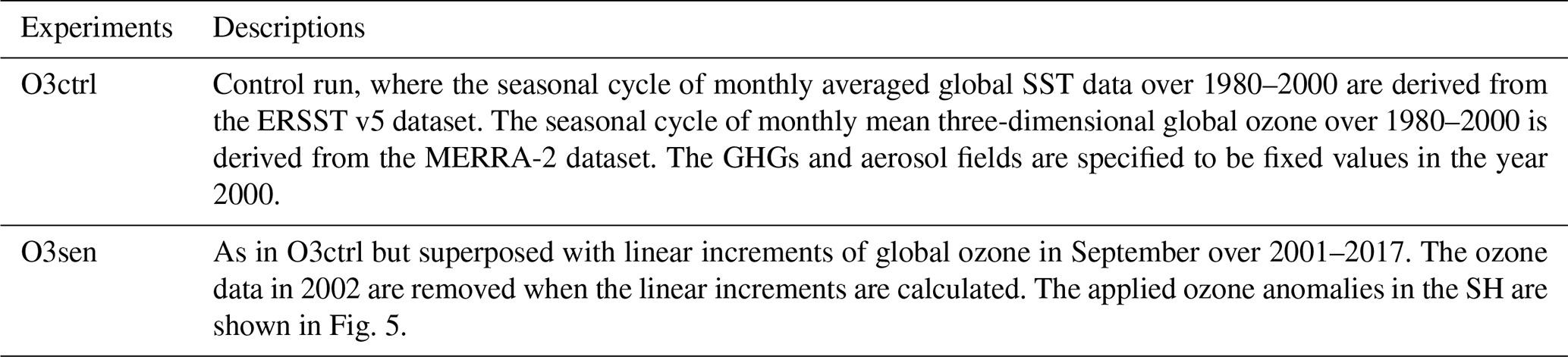
Control experiments and sensitivity experiments are conducted to investigate the responses of Antarctic stratospheric wave activities to SST trends and the ozone recovery trend in early austral spring. For the experiments of SST trends, monthly mean global SST during 1980–2000 derived from the ERSST v5 dataset is used as the SST forcing field in the control experiment (sstctrl). For the four sensitivity experiments (sstNH, sstSH, ssttrop, and sstSHtrop), linear increments of SST in different regions in September during 2000–2017 are used as the forcing field. Ozone, aerosols, and greenhouse gases (GHGs) in the control experiment and the four sensitivity experiments all have the fixed values from the year 2000. For the experiments of ozone recovery trend, monthly mean three-dimensional global ozone during 1980–2000, derived from the MERRA-2 dataset, is used as the ozone forcing field in the control experiment (O3ctrl). The sensitivity experiment (O3sen) is forced by linear increments of ozone in September during 2001–2017. The SSTs in O3ctrl and O3sen both are monthly mean global SST during 1980–2000. The aerosol and GHG values in the year 2000 are used. These experiment configurations are summarized and listed in Tables 1 and 2.

Table 1 Configurations of experiments for SST trends.

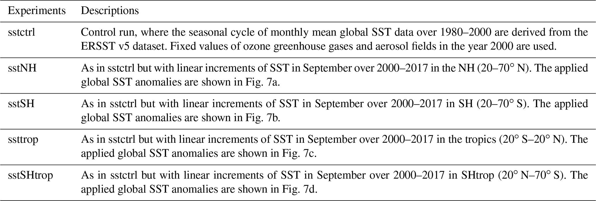
Table 2 Configurations of experiments for the ozone recovery trend.

First, we run the FWSC component to randomly generate different initial conditions for 120 years with a free run. Then, each experiment includes 100 ensemble members that run from July to September and forced by these initial conditions from the 21st year to the 120th year in July. The forcing fields of SST and ozone are only superposed from July to September. July and August are taken as the spin-up time, and simulations during this period are discarded. The ensemble mean in September derived from these 100 ensemble members is regarded as the final result of each experiment. A similar approach is implemented for sensitivity experiments, in which the forcing fields superposed only in certain months. The same approach has been used in previous studies (e.g., Zhang et al., 2018).

3 Trend of planetary wave activities in early austral spring

Figure 1 shows the trends of stratospheric planetary wave activities in the Southern Hemisphere in September during 1980–2000 and 2000–2017, respectively. Note that the vertical E–P flux entering into the stratosphere over 50–70^∘ S in September has been increasing during 1980–2000 and is accompanied by an intensified wave flux convergence in the upper stratosphere (Fig. 1a) that is mainly contributed by the wave 1 component (Fig. 1b). This feature implies that the stratospheric planetary wave activities have strengthened in early austral spring during 1980–2000. A similar result has been reported in previous studies (Hu and Fu, 2009; Lin et al., 2009). During 2000–2017, however, a vertical propagation of stratospheric E–P flux weakened over the subpolar region of the Southern Hemisphere, which was accompanied by intensified wave flux divergence in the upper stratosphere (Fig. 1d) that was mainly contributed by the wave 1 component (Fig. 1e), while the wave 2 component also made certain contributions (Fig. 1f). Similar features also appear in August but are not as significant as those in September (Fig. S1 in the Supplement). For this reason, hereafter we focus on the features in September.

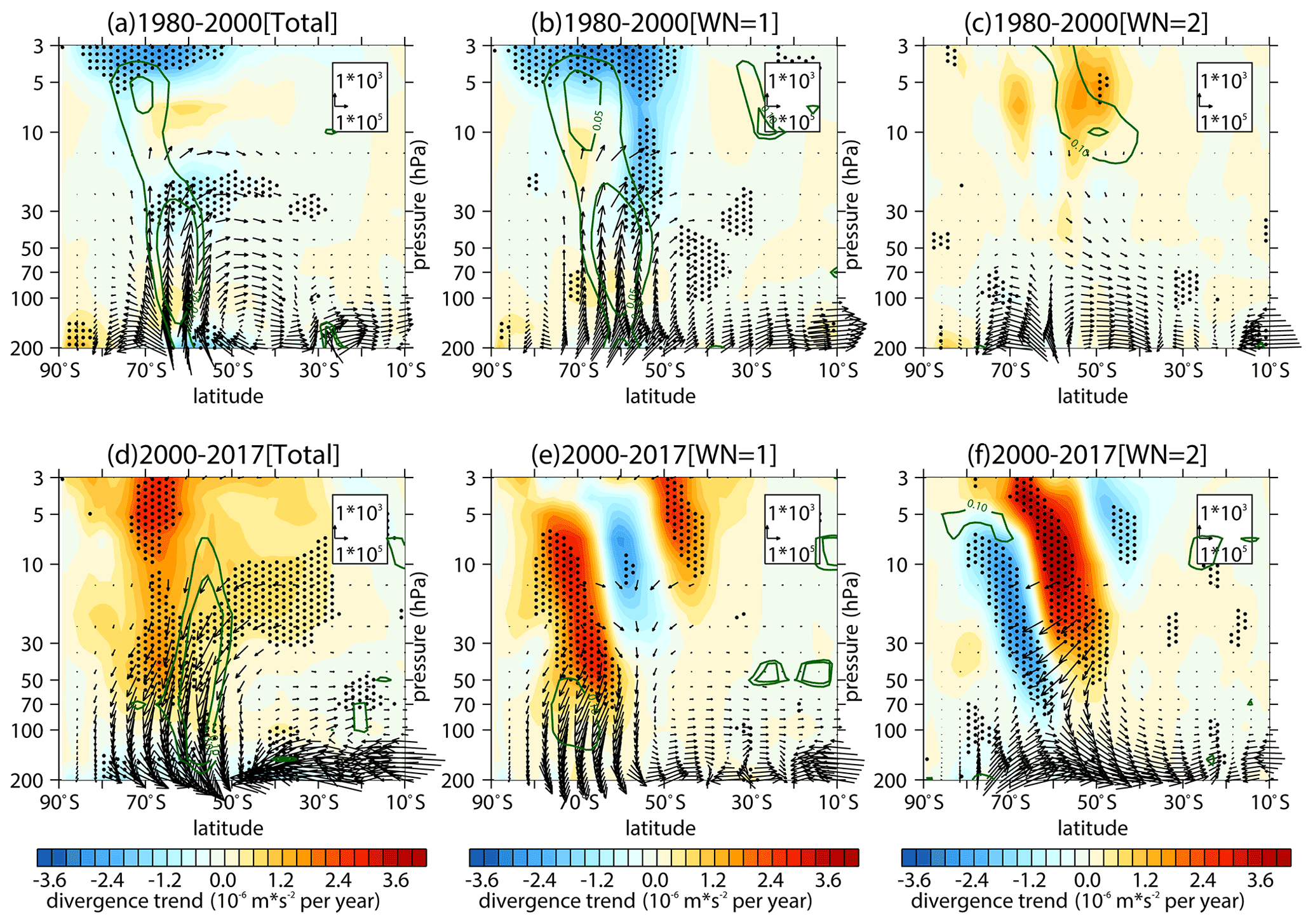
Figure 1 Trends in the Southern Hemisphere (a, d) stratospheric E–P flux (arrows; units of horizontal and vertical components are 10⁵ and 10³ kg s⁻² yr⁻¹, respectively) and its divergence (shading) with their (b, e) wave 1 components and (c, f) wave 2 components over (a, b, c) 1980–2000 and (d, e, f) 2000–2017 in September, as derived from the MERRA-2 dataset. The stippled regions indicate the trend of the E–P flux divergence significant at/above the 90 % confidence level. The green contours from outside to inside (corresponding to p=0.1 and 0.05) indicate the trend of vertical E–P flux significant at the 90 % and 95 % confidence level, respectively.

The SSW that occurred in 2002 was accompanied by large upward wave fluxes in the stratosphere, which is extremely rare in history and has been studied extensively in previous studies (e.g., Baldwin et al., 2003; Nishii and Nakamura, 2004; Newman and Nash, 2005). Since the period with a negative trend of the stratospheric vertical wave flux is short, it is necessary to further investigate whether such a negative trend is artificially influenced by the single year of 2002. Therefore, following Banerjee et al. (2020), we use a change point method to test the significance of the trend during various periods, based on four reanalysis datasets (ERA-Interim, MERRA-2, JRA-55, and NCEP-2). Figure 2a (including the year 2002) and b (excluding the year 2002) display the time series of the area-weighted vertical stratospheric wave flux (Fz) over the Southern Hemisphere subpolar region obtained from different reanalysis datasets. Note that the wave flux time series obtained from the four reanalysis datasets all present a positive trend from the early 1980s to the early 2000s and a negative trend from the early 2000s to present, regardless of whether the extreme value in 2002 is removed or not. The correlation coefficients of the time series between these reanalysis datasets are above 0.9 and statistically significant (Table 3), suggesting that the time series derived from different datasets are consistent with each other. Figure 2c–f show the trends and corresponding confidence intervals calculated with the four different beginning years (1980, 1981, 1982, and 1983), the four different ending years (2015, 2016, 2017, and 2018), and the change point years from 1998 to 2013. The trends and confidence intervals in Fig. 2g–j are the same as those in Fig. 2c–f, except that the extreme value in 2002 is removed. The positive trend from the early 1980s to the 21st century remains significant, regardless of different beginning years and ending change point years (Fig. 2c–j). However, Fig. 2c–f and g–j indicate that the positive value of the trend is decreasing gradually when the period is prolonged, which is apparently attributed to the negative trend with the beginning change point year of around the year 2000. Although the negative trend from the change point year to the ending year becomes less significant when the value in 2002 is removed, it remains significant in some periods, which is also illustrated in the diagrams of latitude pressure profiles (Fig. S2). Therefore, the weakening of stratospheric wave activities in early austral spring since the early 2000s has been robust. In this paper, we take the year 2000 as the beginning year of the weakening trend to simplify descriptions in the following discussion.

Table 3 Correlations of stratospheric vertical wave flux time series (area weighted from 100 to 30 hPa over 70–50^∘ S) between different reanalysis dataset.

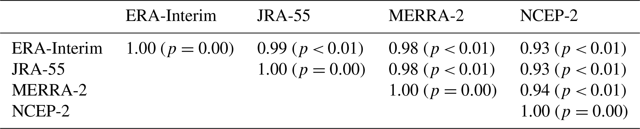
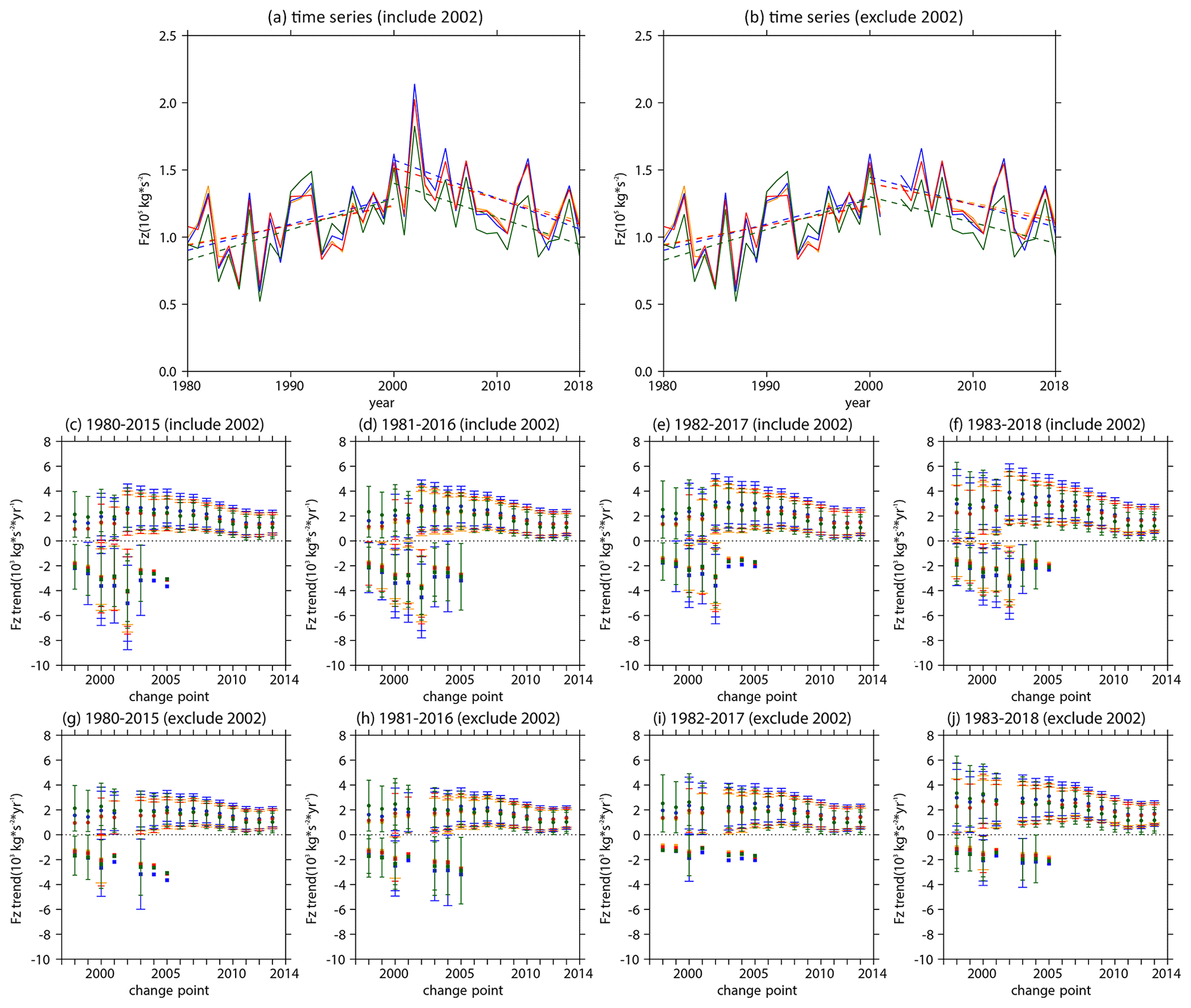
Figure 2 (a) The mean time series (solid lines) and piecewise (during 1980–2000 and 2000–2018) linear regressions (dashed lines) of vertical E–P flux area weighted from 100 to 30 hPa over 70–50^∘ S in September during 1980–2018 as derived from ERA-Interim (yellow), MERRA-2 (blue), JRA-55 (red), and NCEP-2 (green). Panel (b) is the same as panel (a), except that the data in 2002 are removed. (c, d, e, f) The trends (dots) and uncertainties (error bars) calculated during various periods using the change point method with different beginning and ending years (titles). Circles and squares in panels (c), (d), (e), and (f) represent positive trends from the beginning years to change point years (x axes) and negative trends from change point years to ending years, respectively. Different colors of the dots and error bars in panels (c), (d), (e), and (f) correspond to colors in panel (a), which represent trends and uncertainties derived from different datasets. The long and short error bars in same color reflect the 95 % and 90 % confidence intervals calculated by two-tailed t test. The error bar is omitted when the significance of the trend is lower than the corresponding confidence level. Negative trends and corresponding uncertainties with the beginning change point in the years after 2005 are also omitted, since the trend value shows a large fluctuation with the shortening of the time series. Panels (g), (h), (i), and (j) are the same as panels (c), (d), (e), and (f), except that the data in 2002 are removed when calculating trends and uncertainties.

Figure 3 shows the trends in tropospheric wave sources in September since the year 2000. There is a significant positive trend of the wave 1 component at 500 hPa geopotential height over the southern Indian ocean and a significant negative trend over the southern Pacific, which form an out-of-phase superposition on its climatology (Fig. 3b). The trend pattern of the wave 2 component is also out of phase with its climatology, although it is not significant (Fig. 3c). The above features are still maintained when the values in 2002 are removed (Fig. S3b, c), implying that the southern hemispheric tropospheric wave sources in early austral spring have weakened since the year 2000, which is also reflected in the decrease in the tropospheric vertical wave flux (Figs. 3d, e; S3d, e).

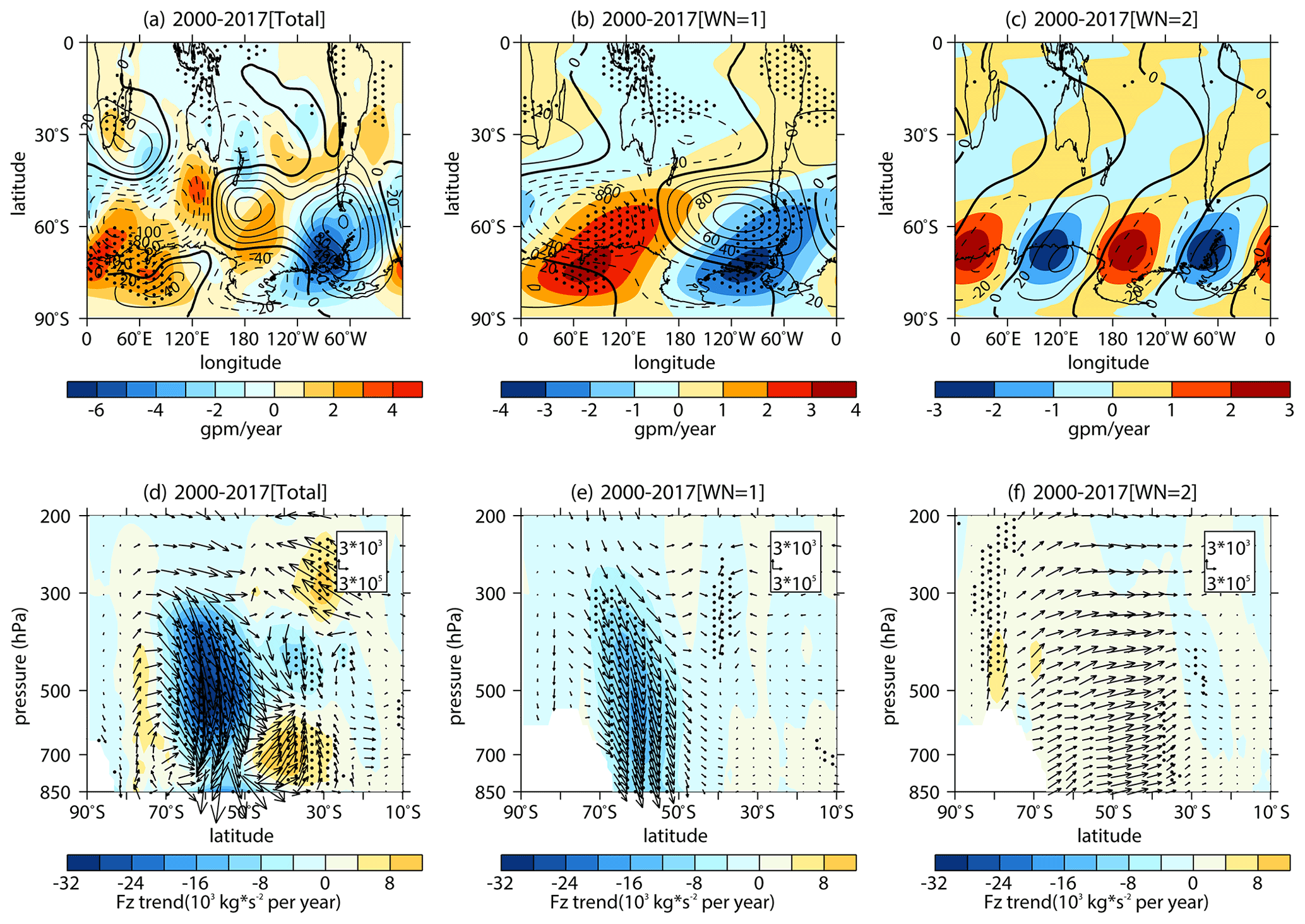
Figure 3 Trends (shading) and climatological distributions (contours with an interval of 20 gpm (geopotential meters); positive and negative values are depicted by solid and dashed lines, respectively; zeroes are depicted by thick solid lines) of southern hemispheric (a) 500 hPa geopotential height zonal deviations, with their (b) wave 1 component and (c) wave 2 component in September during 2000–2017, as derived from the MERRA-2 dataset. Trends of the southern hemispheric (d) tropospheric E–P flux (arrows; units of horizontal and vertical components are 3 × 10⁵ and 3 × 10³ kg s⁻² yr⁻¹, respectively) and its vertical component (shading), with their (e) wave 1 component and (f) wave 2 component in September during 2000–2017, as derived from the MERRA-2 dataset. The stippled regions represent the trend significant at/above the 90 % confidence level.

4 Response of Antarctic stratospheric wave activity to ozone recovery

Previous studies have suggested that ozone depletion and recovery are important to the climate shift that occurred around the year 2000 in the Southern Hemisphere during austral summer (e.g., Son et al., 2008; Thompson et al., 2011; Barnes et al., 2014; Banerjee et al., 2020). The impacts of stratospheric ozone changes on Antarctic wave propagation during austral summer has also been examined in previous studies (e.g., Hu et al., 2015). However, whether ozone recovery in September explains the weakening of stratospheric planetary waves during the same month remains unclear. The correlation between the detrended time series of the September Antarctic total column ozone (TCO) derived from SBUV and stratospheric vertical wave flux (Fz) is 0.70 (p=0.0011) during 2000–2017. The increase in wave activity in the polar stratosphere causes heating effects and suppresses the formation of PSCs and, hence, slows down the ozone depletion (e.g., Shen et al., 2020a). Therefore, the Antarctic ozone and stratospheric wave activity show a statistically significant positive correlation. Theoretically, heating effects caused by ozone recovery in the Antarctic stratosphere may also decelerate the Antarctic stratospheric polar vortex and induce more waves to propagate into stratosphere (Andrews et al., 1987; Holton, 2004). These preliminary analysis cannot verify that the ozone recovery is responsible for the weakening of stratospheric wave activity. The role of ozone recovery in stratospheric wave changes needs to be further explored by model simulations. In this section, we use a group of time slice experiments (O3ctrl and O3sen) to address this issue.

Figure 4 shows the time series and piecewise trends of the September TCO in the Antarctic during 1980–2017. As reported by previous studies (e.g., Angell and Free, 2009; Banerjee et al., 2020; Krzyścin, 2012; Solomon et al., 2016; WMO, 2011; Zhang et al., 2014), the Antarctic ozone show a significant decline during 1980–2000 (Fig. 4a, b, c) and a slight recovery during 2001–2017 (Fig. 4a, d, e). The recovery trend is calculated with the data in 2002 removed because the large poleward transport induced by SSW in 2002 leads to extreme values of ozone (e.g., Solomon et al., 2016). In addition, the correlation of TCO between the MERRA-2 and SBUV datasets is 0.61 (p=4.5 × 10⁻⁵), suggesting the changes of TCO derived from the reanalysis dataset, and the observations have a good consistency. Thus, in order to obtain a three-dimensional structure of ozone changes, the ozone data from MERRA-2 are used to make forcing fields for CESM. As described in Sect. 2, a control experiment (O3ctrl) forced by climatological ozone and a sensitivity experiment forced by the linear increment of global ozone in September during 2001–2017 are conducted to explore the impacts of ozone recovery. The pattern of ozone forcing fields is similar to its trend patterns (Figs. 4d, e; 5a, b). Other details of these two experiments have been given in Sect. 2 and Table 2.

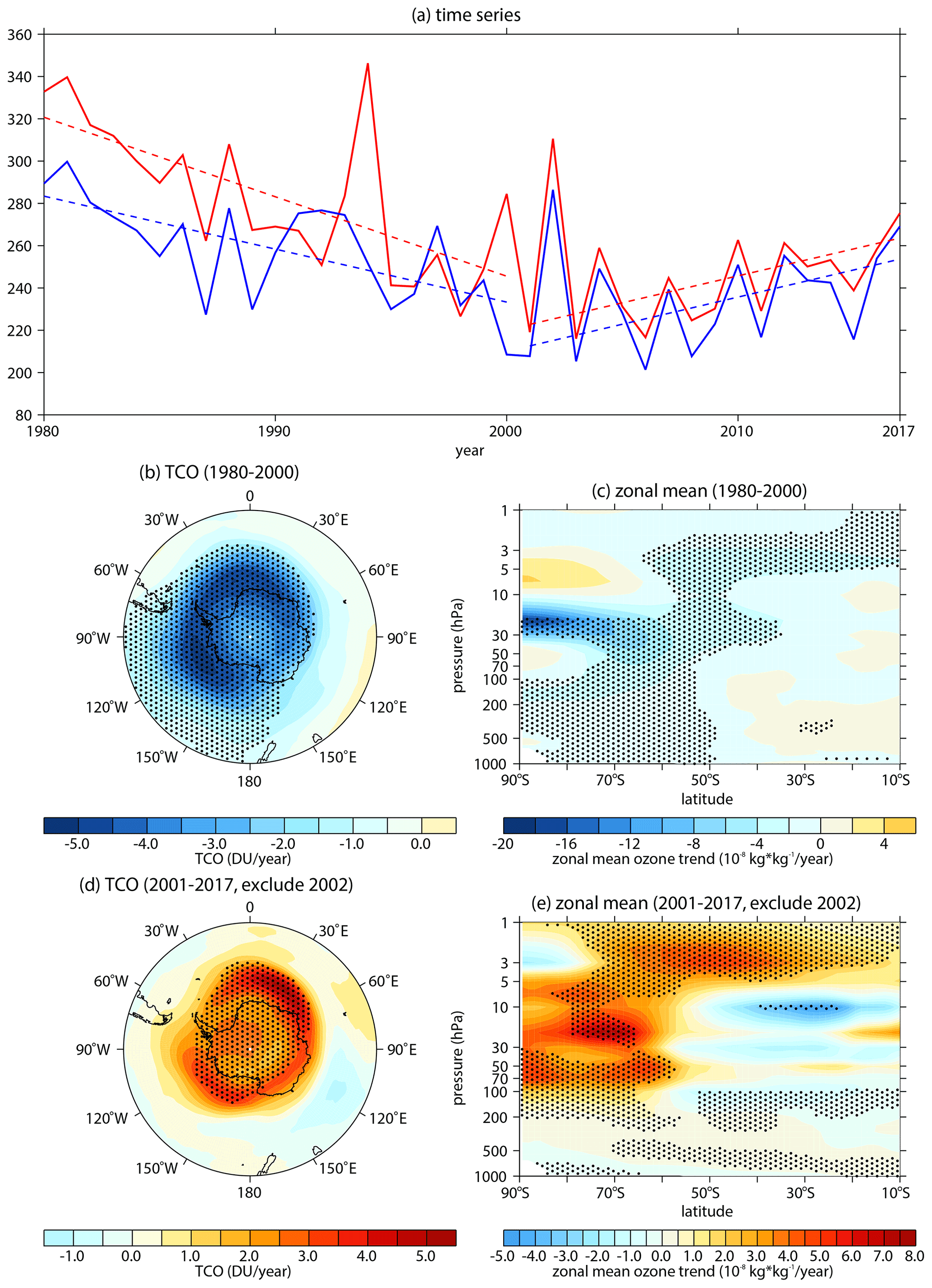
Figure 4 (a) Time series (solid lines) of area-weighted total column ozone (TCO) over 60 to 90^∘ S as derived from the MERRA-2 (red) and SBUV (blue) datasets. The dashed lines represent linear regression of TCO. (b, d) The TCO trends in September during 1980–2000 (b) and 2001–2017 (d) as derived from the MERRA-2 dataset. The outermost latitudes in panels (c, d) are both 40^∘ S. (c, e) The zonal mean ozone trends on the latitude pressure profile in September during 1980–2000 (c) and 2001–2017 (e) as derived from the MERRA-2 dataset. The stippled regions in panels (b)–(e) represent trends significant at/above the 90 % confidence level. Data from 2002 are removed when trends, regressions, and significances are calculated in this figure.

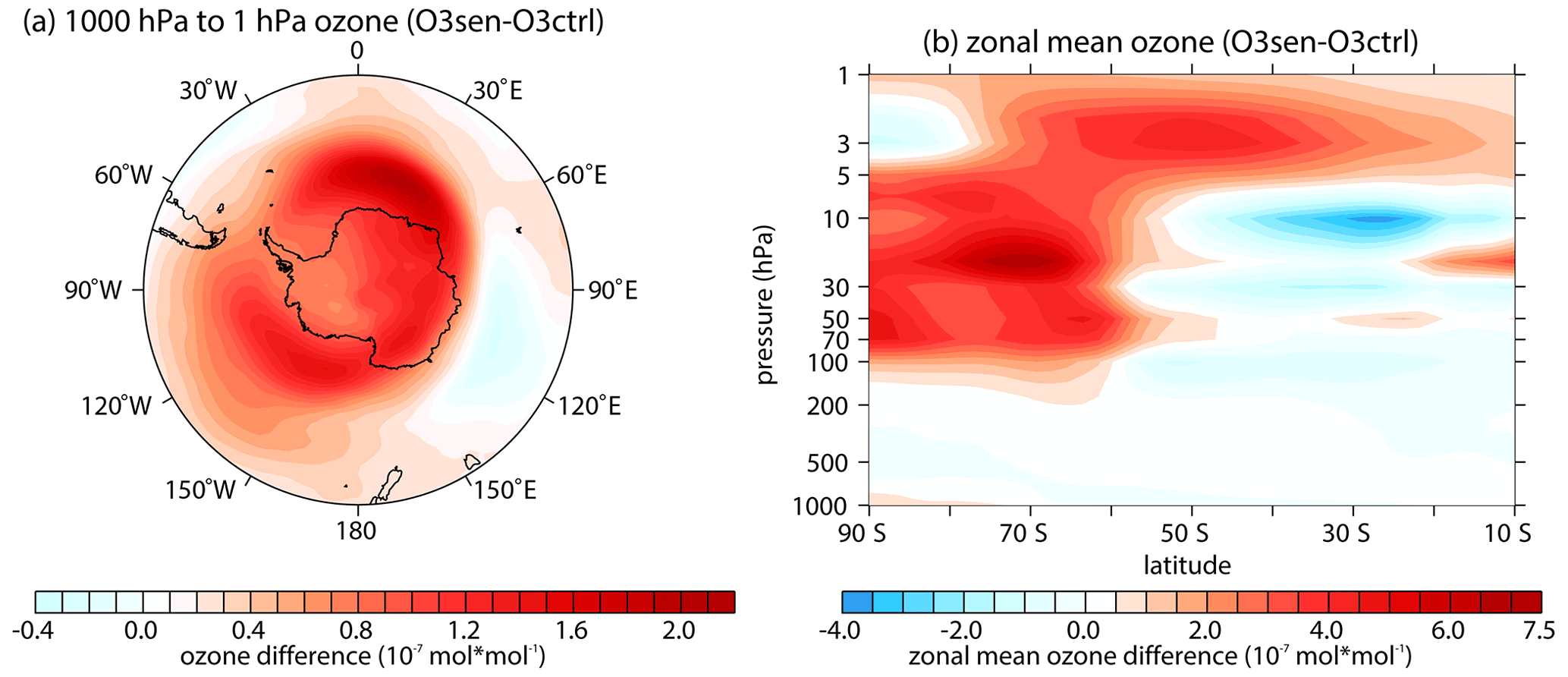
Figure 5 (a) Difference in the horizontal ozone forcing field averaged from 1000 to 1 hPa between O3sen and O3ctrl. The outermost latitude in panel (a) is 40^∘ S. (b) Zonal mean difference in the ozone forcing fields on latitude pressure profile in the Southern Hemisphere between O3sen and O3ctrl.

Figures 6 and 7 show the responses of the wave activity and wave propagation environment forced by O3sen. Note that the significant ozone recovery over the South Pole mainly appears in the lower stratosphere (about 200 to 50 hPa; Fig. 4e). In most southern polar regions, from 50 to 3 hPa, the ozone recovery is not significant (Fig. 4e). The features are attributed to limitation of the emission of ozone-depleting substances (ODSs) and the reduction in heterogeneous reactions on PSCs, which mainly distribute in the lower stratosphere (e.g., Solomon, 1999). Ozone recovery in the polar lower stratosphere absorbs more ultraviolet radiation and causes cooling in the Antarctic troposphere (Fig. 6b). To maintain the thermal balance, zonal wind accelerates below 200 hPa over 60–70^∘ S (Fig. 6a).

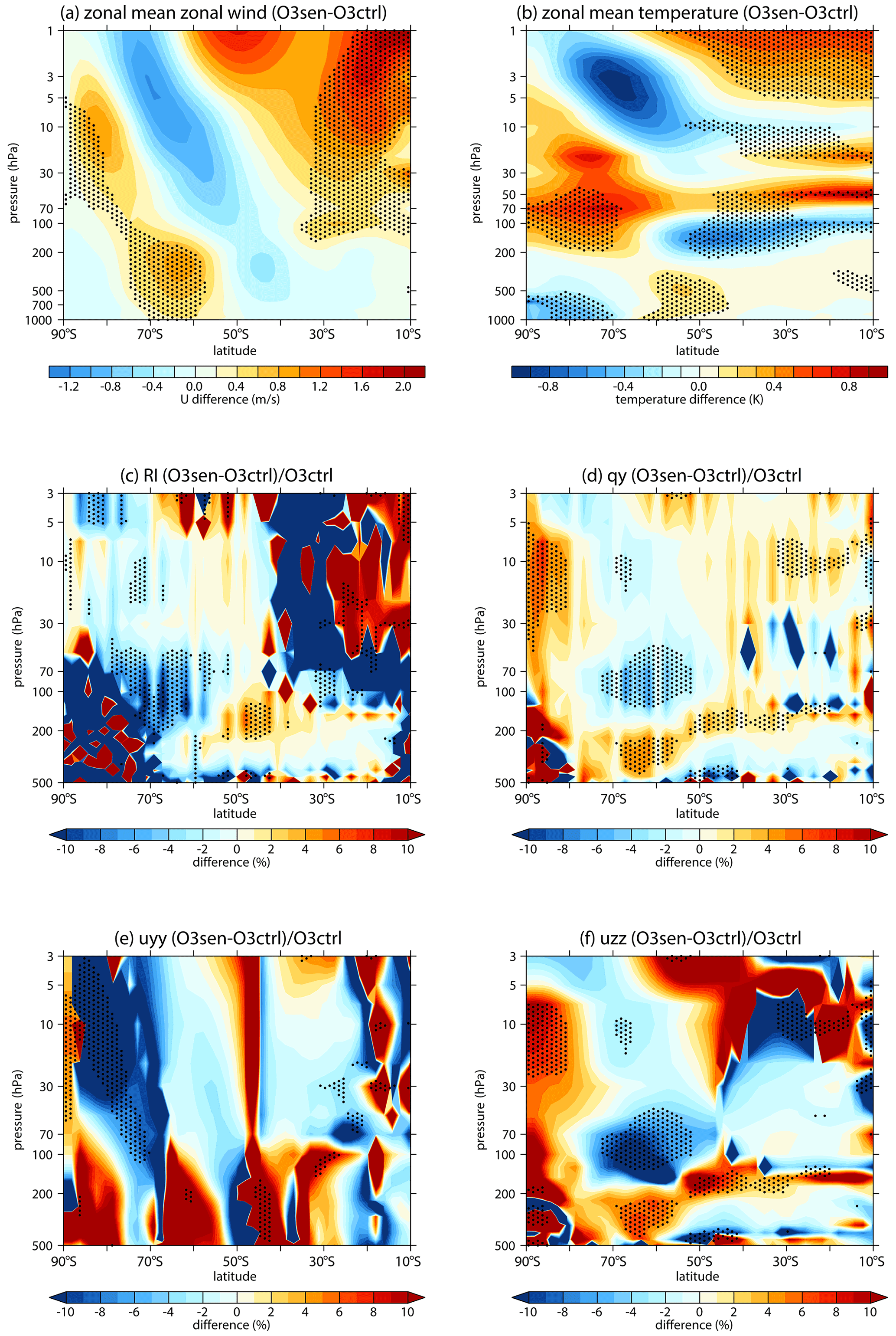
Figure 6 Differences in the (a) zonally averaged zonal wind, (b) zonally averaged temperature, (c) refractive index, (d) $a^{\mathrm{2}}{\overline{q}}_{\mathit{\phi }}$, (e) $-{\left[\frac{(\overline{u}\cos \mathit{\phi }{)}_{\mathit{\phi }}}{\cos \mathit{\phi }}\right]}_{\mathit{\phi }}$ (uyy term), and (f) $-\frac{a^{\mathrm{2}}{f}^{\mathrm{2}}}{{\mathit{\rho }}_{\mathrm{0}}}{\left({\mathit{\rho }}_{\mathrm{0}}\frac{{\overline{u}}_z}{N^{\mathrm{2}}}\right)}_z$ (uzz term) between O3sen and O3ctrl. The stippled regions represent the difference significant at/above 90 % confidence level.

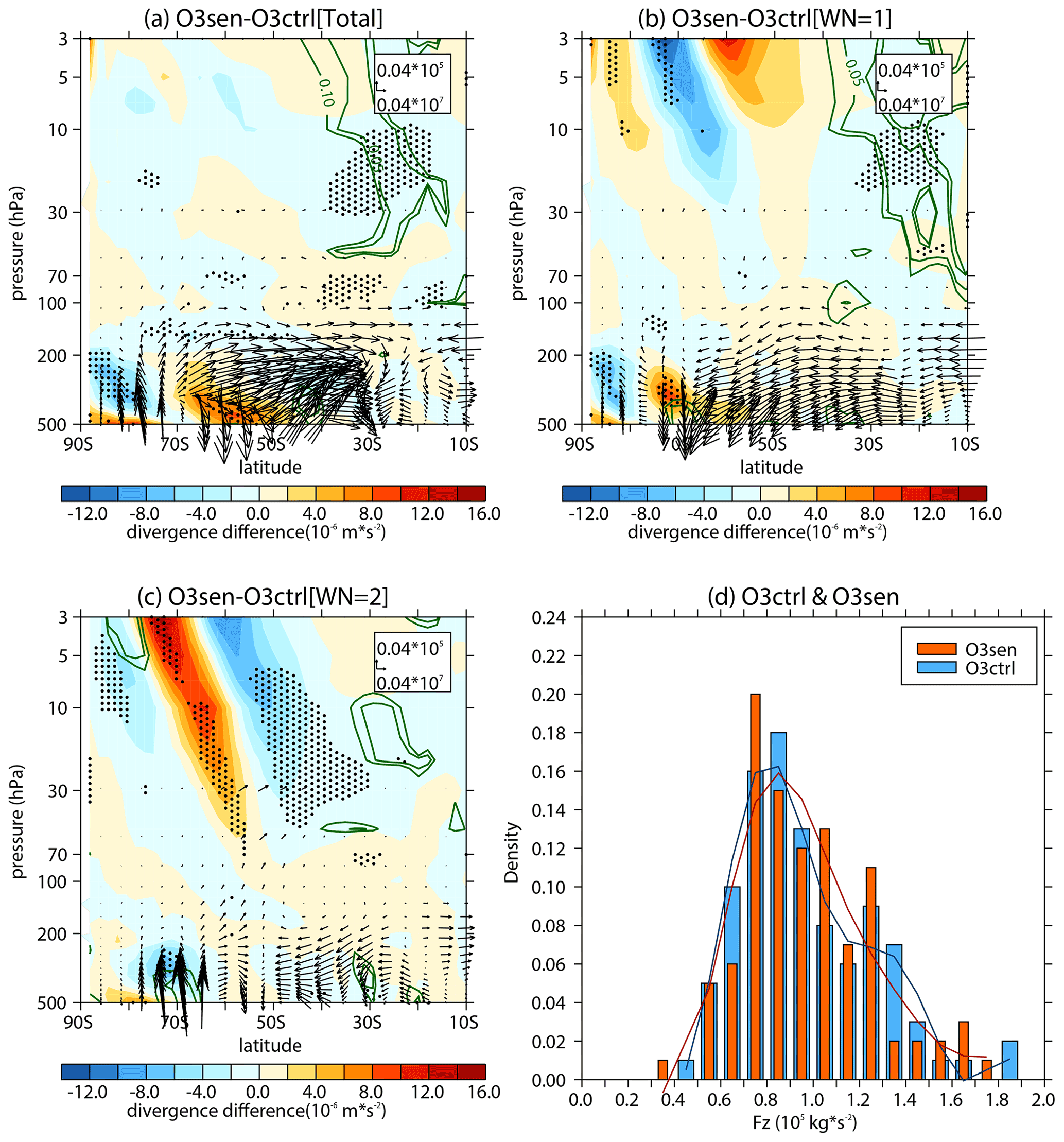
Figure 7 Differences in the (a) stratospheric E–P flux (arrows; units in horizontal and vertical components are 0.04 × 10⁷ and 0.04 × 10⁵ kg s⁻², respectively) and its divergence (shading) with their (b) wave 1 component and (c) wave 2 component between the sensitivity experiment (O3sen) and the control experiment (O3ctrl). The stippled regions represent the mean differences in the E–P flux divergence significant at/above the 90 % confidence level. The green contours from outside to inside (corresponding to p=0.1 and 0.05) represent the mean differences in the vertical E–P flux significant at the 90 % and 95 % confidence levels, respectively. (d) Frequency distributions (pillars; blue for O3ctrl and orange for O3sen) of vertical E–P flux (Fz; area weighted from 200 to 10 hPa over 70–50^∘ S) and its five-point low-pass filtered fitting curves (solid lines; blue for O3ctrl and red for O3sen) derived from 100 ensemble members.

The changes in the zonal wind and temperature forced by the ozone recovery induce changes in the wave propagation environment. The refractive index (RI) is a good matric to reflect the atmosphere state for wave propagation. Theoretically, planetary waves tend to propagate into large RI regions (Andrews et al., 1987). The responses of RI and its terms are shown in Fig. 6c–f. Note that the second term of RI does not change with atmospheric state, and the third term of RI is insignificant compared to the first term (Hu et al., 2019). Previous studies indicate that changes in zonal mean potential vorticity meridional gradient ${\overline{q}}_{\mathit{\phi }}$ could explain the changes in RI in the middle and high latitudes (e.g., Hu et al., 2019; Simpson et al., 2009). Consistent with these studies, the pattern of ${\overline{q}}_{\mathit{\phi }}$ shows some similarity with pattern of RI (Fig. 6c, d), especially in lower stratosphere over subpolar regions (Fig. 6c, d). According to the Eq. (5), the first term of ${\overline{q}}_{\mathit{\phi }}$ does not change with the atmospheric state. Therefore, the second term ($-{\left[\frac{(\overline{u}\cos \mathit{\phi }{)}_{\mathit{\phi }}}{\cos \mathit{\phi }}\right]}_{\mathit{\phi }}$; hereafter the uyy term or barotropic term) and the third term ($-\frac{f^{\mathrm{2}}}{{\mathit{\rho }}_{\mathrm{0}}}{\left({\mathit{\rho }}_{\mathrm{0}}\frac{{\overline{u}}_z}{N^{\mathrm{2}}}\right)}_z$; hereafter the uzz term or baroclinic term) are investigated. Note that the pattern of responses in the baroclinic term is similar with ${\overline{q}}_{\mathit{\phi }}$ (Fig. 6d, f). The uzz term also can be written as $\left(\frac{f^{\mathrm{2}}}{H{N}^{\mathrm{2}}}+\frac{f^{\mathrm{2}}}{N^{\mathrm{4}}}\frac{\mathrm{d}{N}^{\mathrm{2}}}{\mathrm{d}z}\right){\overline{u}}_z-\frac{f^{\mathrm{2}}}{N^{\mathrm{2}}}{\overline{u}}_{zz}$. Meanwhile, zonal wind acceleration in the upper troposphere weakens the vertical shear of u (${\overline{u}}_z)$ around 200 hPa over subpolar regions, inducing a decrease in the baroclinic term and RI in upper troposphere and lower stratosphere (UTLS) over 60–70^∘ S (Fig. 6d, f). The response of RI induces a slight decrease in the vertical wave flux in UTLS over subpolar regions (Fig. 7a), which is mainly contributed by its wave 1 component (Fig. 7b). However, the changes in the wave activity in UTLS are not significant in the ensemble mean of the simulations (Fig. 7a, b, c). Meanwhile, note that the responses of zonal wind and temperature to ozone recovery are not significant above 50 hPa over subpolar regions (Fig. 6a, b), thus inducing negligible changes in the wave propagation environment (Fig. 6c) and wave activity (Fig. 7) in the middle and upper stratosphere.

In a word, the significant ozone recovery in the Antarctic lower stratosphere changes the wave propagation in upper troposphere and lower stratosphere to some extent. However, these weak responses still cannot explain the significant decrease of stratospheric wave flux in September.

5 Role of SST trends in the weakening of Antarctic stratospheric wave activities

In this section, we further explore the factors responsible for the weakening of tropospheric wave sources and stratospheric wave activities since the early 2000s in early austral spring. Many studies reported that SST variations can affect stratospheric climate (e.g., Li, 2009; Hurwitz et al., 2011; Lin et al., 2012; Hu et al., 2014, 2018; Tian et al., 2017; Xie et al., 2020). Hu and Fu (2009) also attributed the strengthened stratospheric wave activities in the Southern Hemisphere to the SST trend from the early 1980s to the early 2000s. Furthermore, global SST in September during 2000–2017 also has a significant trend. The significant warming pattern is mainly found over the southern Indian ocean, the southern Atlantic ocean, the eastern and western equatorial Pacific, and the western equatorial and northern Atlantic ocean (Fig. 8b). A significant cooling pattern is located over the southeastern Pacific (Fig. 8b). In addition, the transitions around the year 2000 exist in the SST time series over some regions. In the southern Indian ocean, SST shows an insignificant trend during 1980–2000 and a significant warming trend during 2000–2017 (Fig. 8c). The subtropical Pacific Ocean in east of Australia is linked with the Pacific–South American (PSA) wave train (e.g., Shen et al., 2020b), and the SST there shows a significant warming trend during 1980–2000 and an insignificant trend during 2000–2017. The SST in the southeastern Pacific shows an insignificant trend during 1980–2000 and significant cooling during 2000–2017 (Fig. 8e). Trends of SST in southern Atlantic Ocean are the opposite during these two piecewise periods, showing significant cooling during 1980–2000 and significant warming during 2000–2017. It is apparent that the spatial pattern of SST trend during 2000–2017 is obviously different from that during 1980–2000 (Fig. 8a, b), which may affect the tropospheric wave sources. Thus, it is necessary to analyze the connection between SST trend and wave activity trend since the early 2000s.

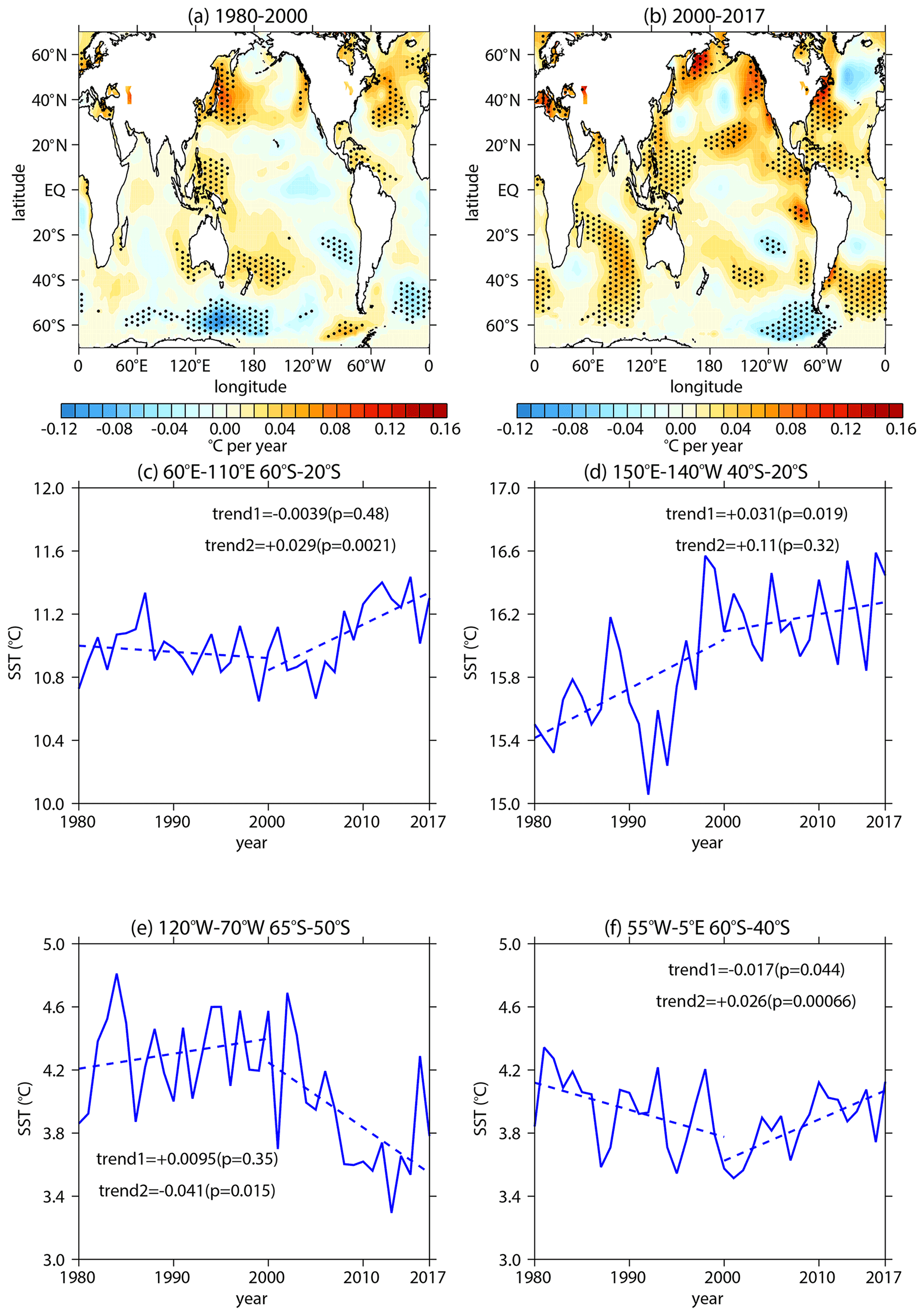
Figure 8 Trends of SST in September over (a) 1980–2000 and (b) 2000–2017 as derived from the ERSST v5 dataset. The stippled regions represent the trends significant at/above the 90 % confidence level. (c–f) Time series (blue solid lines) of SST during 1980–2017 over different regions (titles). The dashed lines represent linear regressions of the SST time series on piecewise periods (1980–2000 and 2000–2017). The labels of trend1 and trend2 in panels (c)–(f) represent the trend coefficients and the corresponding significances (in parentheses) over 1980–2000 and 2000–2017, respectively.

Figure 9 Trend significance of the first three SST principal components (PCs) in (a) the extratropical Southern Hemisphere (SH; 70–20^∘ S), (b) the tropics (TROP; 20^∘ S–20^∘ N), (c) the extratropical Northern Hemisphere (NH; 20–70^∘ N), (d) the extratropical Southern Hemisphere and the tropics (SHtrop; 70^∘ S–20^∘ N), (e) the extratropical Northern Hemisphere and the tropics (NHtrop; 20^∘ S–70^∘ N), (f) the globe (70^∘ S–70^∘ N), and the corresponding (g, h, i, j, k, l) correlation significances between them and the vertical E–P flux (Fz; area weighted from 100 to 30 hPa over 70–50^∘ S) during different beginning years (x axes) and ending years (y axes). The red and blue dots indicate that a positive and negative trend or correlation coefficient are significant, respectively. The black dots indicate that the trends or correlation coefficients are not significant. The stars indicate that the trends and the corresponding correlation coefficients are both significant. Each panel is divided into three regions, from bottom to top, corresponding to the first, second, and third PCs, respectively. The criterion to distinguish whether the trends and correlations are significant or not is the 90 % confidence level.

Figure 9 shows the significance of the trend of the principle component (PC) time series of the SST in different regions (Fig. 9a–f) and the significance of the correlations (Fig. 9g–l) between the PC time series and Fz in September during various periods. The trend of the PC1 time series in the SH region is significant during serval periods (Fig. 9a), while the correlation between PC1 and Fz is only significant with the particular ending year of 2015 (Fig. 9g). This feature suggests that the connection between the SST trend in SH region and the trend of stratospheric wave activity is not robust. The correlation between trend of stratospheric wave activity and that of SST in the TROP or NH regions is also weak (Fig. 9e, f). As for the combined regions, note that the PC2 time series in the SHtrop region has a significant trend (Fig. 9d), and the correlation between the PC2 time series in SHtrop and Fz with the beginning year of around the year 2000 is also significant (Fig. 9j), regardless of the different ending years. This feature implies that the extratropical Southern Hemisphere and tropical SST has a robust connection with stratospheric wave activities in early austral spring since the early 2000s. The correlations between Fz and all PC time series in the NHtrop (Fig. 9k) and globe (Fig. 9l) regions are not as robust as those between Fz and PC2 time series in the SHtrop region (Fig. 9j), indicating that the connection between SST trends in the extratropical Northern Hemisphere and the trend of stratospheric wave activity is weak.

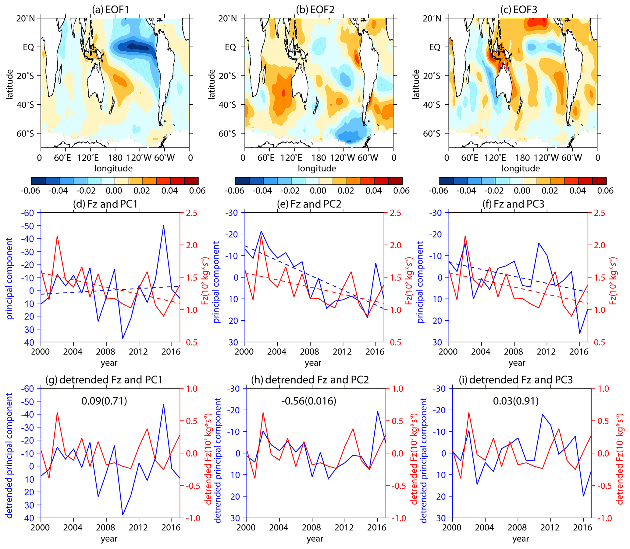
Figure 10 (a, b, c) The first three EOF patterns of SST in the SHtrop region. (d, e, f) The original time series of the first three principle components (PCs; blue solid lines correspond to left inverted y axes) and stratospheric vertical E–P flux (Fz; area weighted from 100 to 30 hPa over 70–50^∘ S; red solid lines correspond to right y axes) in September during 2000–2017. The blue and red dashed lines in panels (d), (e), and (f) represent the linear regressions of PC time series and Fz time series, respectively. The meaning of panels (g), (h), and (i) is the same as panels (d), (e), and (f), correspondingly, except for the detrended time series. The numbers without (and in) parentheses in panels (g), (h), and (i) represent the correlation coefficients between the detrended PC time series and Fz time series and the corresponding p values calculated by the two-tailed t test, respectively.

Figure 10 shows the first three EOF modes of the September SST in the SHtrop region during 2000–2017. The second mode (Fig. 10b) shows a great similarity to the spatial pattern of the SST trend (Fig. 8b), and the corresponding PC2 time series also has a significant trend (slope = 1.71; p<0.01). The correlation between PC2 and Fz is significant ($r=-$0.56; p=0.016), and the correlation coefficient remains significant ($r=-$0.46; p=0.065) at the 90 % confidence level when the value in 2002 is removed. This result suggests that the SST trend in the SHtrop region is closely related to the recent weakening of the stratospheric wave activities. The first EOF mode is similar to IPO (Fig. 10a), and its corresponding principal component is significantly correlated ($r=-\mathrm{0}$.98; p<0.01) with the unfiltered IPO index. However, it shows no significant trend (Fig. 10d) and has no significant correlation (Fig. 10g) with the stratospheric wave flux, implying that the link between the IPO phase change at around the year 2000 (e.g., Trenberth and Fasullo, 2013) and the weakening of Antarctic stratospheric wave activities is weak. The correlation between PC3 and Fz is also not significant (Fig. 10i). Therefore, it is possible that the combined effect of the SST trend (the second EOF mode) in the tropical and extratropical Southern Hemisphere has led to the weakening of stratospheric wave activities in early austral spring since the early 2000s.

6 Simulated changes in Antarctic stratospheric wave activities forced by SST trends

The analysis in Sect. 5 suggests that the SST changes in the SHtrop region may contribute to the weakening of the southern hemispheric stratospheric wave activities. Here, numerical experiments sstNH, sstSH, ssttrop, and sstSHtrop, forced by linear increments of SST in September during 2000–2017 (Fig. 11; more details can be found in Sect. 2), are conducted to verify the results presented in Sect. 5.

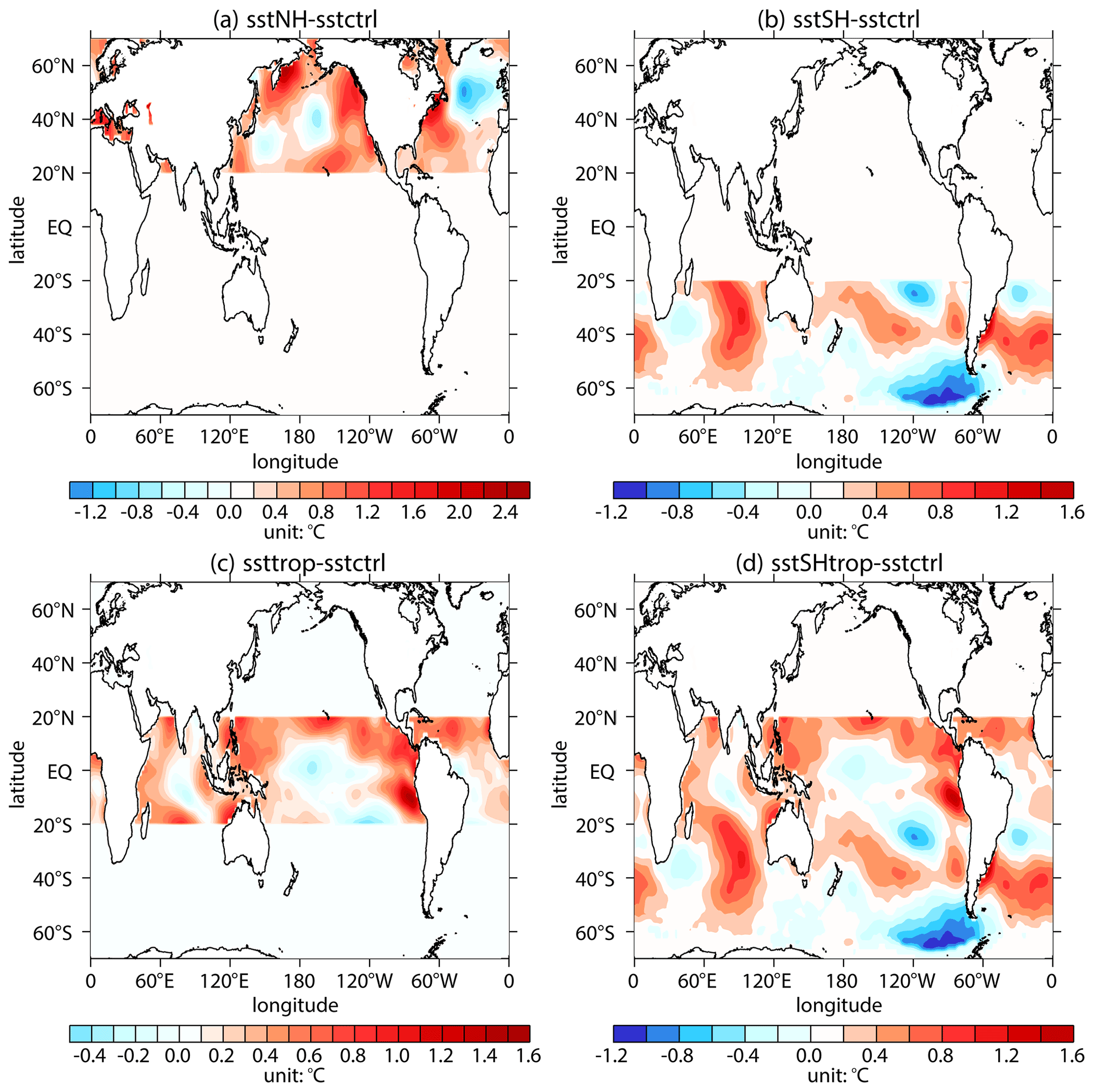
Figure 11 Differences in the SST forcing field between sensitivity experiments (a sstNH; b sstSH; c ssttrop; d sstSHtrop) and the control experiment (sstctrl).

Figure 12 Differences (shading) in the (a, d, g, j) 500 hPa geopotential height zonal deviations with their (b, e, h, k) wave 1 component and (c, f, i, l) wave 2 component between sensitivity experiments (a, b, c sstNH; d, e, f sstSH; g, h, i ssttrop; j, k, l sstSHtrop) and the control experiment (sstctrl). The mean distributions (contours with an interval of 20 gpm; positive and negative values are depicted by solid and dashed lines, respectively; zeroes are depicted by thick solid lines) of them are derived from the control experiment. The stippled regions represent the mean difference significant at/above the 90 % confidence level.

Figure 12 shows the simulated response of 500 hPa geopotential height to SST changes in different regions. The climatological distributions of the wave 1 component (Fig. 12b, e, h, k) and the wave 2 component (Fig. 12c, f, i, l) from the simulations are consistent with that from reanalysis dataset (Fig. 3b, c), indicating that the model can capture spatial distributions of the atmospheric waves well. Note that the wave 1 and wave 2 anomalies simulated with SST changes in SH, TROP, and SHtrop are all significant. They superpose on the corresponding climatological patterns in an out-of-phase style (Fig. 12e, f, h, i, k, l), indicating that the changes in SST in SH, TROP, and SHtrop lead to a weakening of tropospheric wave sources in the extratropical Southern Hemisphere. However, the predominate wave 1 component of the 500 hPa geopotential height anomaly in the extratropical Southern Hemisphere forced by the experiment with NH SST change is relatively weak (Fig. 12b). This feature suggests that the SST changes in extratropical Northern Hemisphere are incapable of inducing a robust response of tropospheric wave sources in the extratropical Southern Hemisphere.

Figure 13 shows the simulated responses of stratospheric wave activities in the Southern Hemisphere to SST changes over different regions. It is apparent that the experiments with SST changes in SH, TROP, and SHtrop show significantly weakened stratospheric wave activities (Fig. 13d, g, j), which are mainly attributed to the responses of the wave 1 component (Fig. 13e, h, k). These results are consistent with the responses of tropospheric wave sources (Fig. 12d, e, g, h, j, k). However, there are no significant anomalies of stratospheric wave flux in the subpolar region in Fig. 13a and b, which is consistent with the response of corresponding tropospheric wave sources (Fig. 12a, b) and the weak correlation between Fz and the PC time series of SST in NH region (Fig. 9i). The result here suggests that the response of Southern Hemisphere stratospheric wave activities to SST trend in NH region is weak.

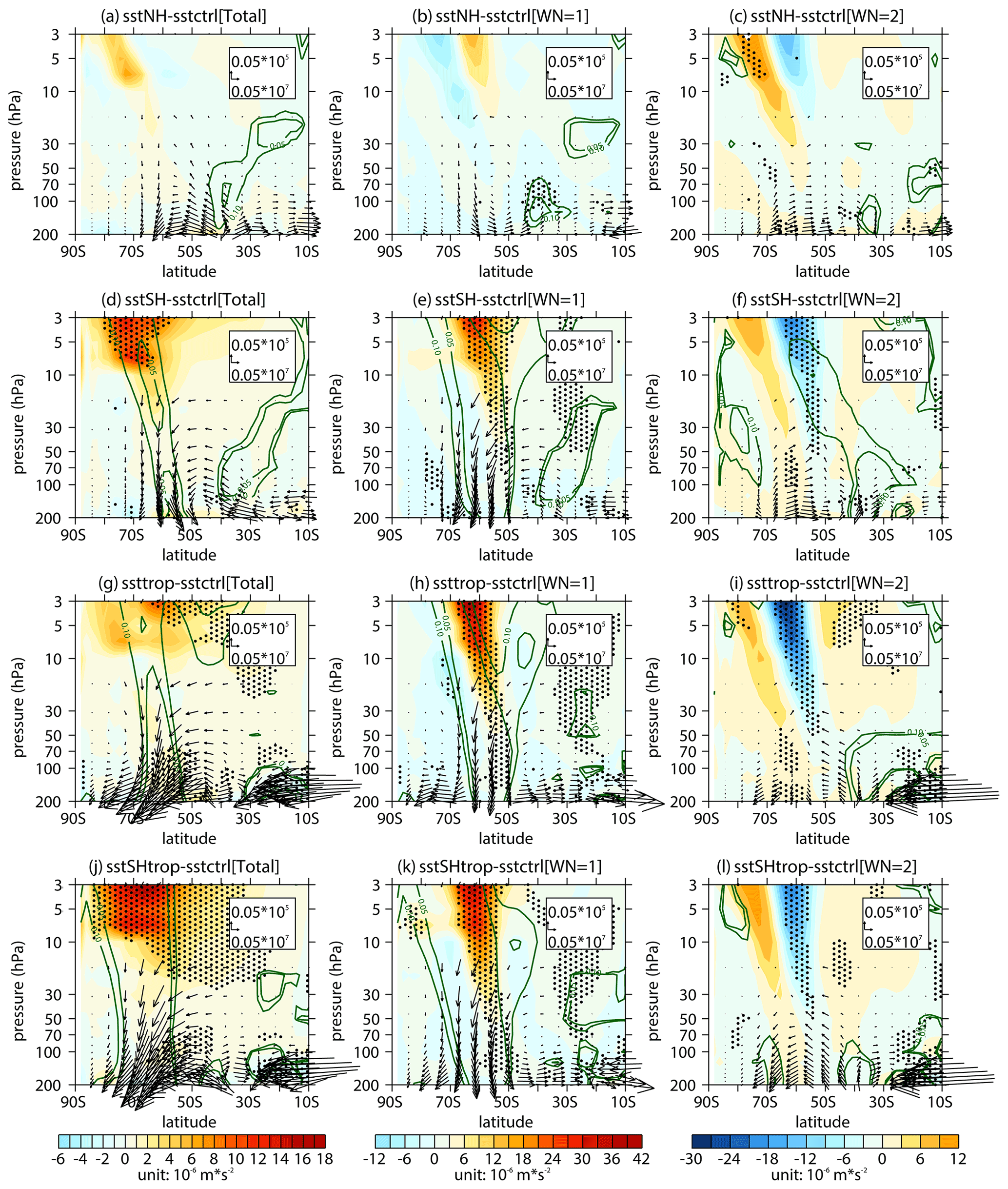
Figure 13 Differences in the (a, d, g, j) stratospheric E–P flux (arrows; units in horizontal and vertical components are 0.05 × 10⁷ and 0.05 × 10⁵ kg s⁻², respectively) and its divergence (shading) with their (b, e, h, k) wave 1 component and (c, f, i, l) wave 2 component between sensitivity experiments (a, b, c sstNH; d, e, f sstSH; g, h, i ssttrop; j, k, l sstSHtrop) and the control experiment (sstctrl). The stippled regions represent the mean differences in the E–P flux divergence significant at/above the 90 % confidence level. The green contours from outside to inside (corresponding to p=0.1 and 0.05) represent the mean differences in the vertical E–P flux significant at the 90 % and 95 % confidence levels, respectively.

The results of stratospheric vertical wave flux over 50–70^∘ S derived from the 100 ensemble members of each experiment are shown in Fig. S4, and the frequency distributions of them are displayed in Fig. 14. Compared to the blue fitting curves, the red fitting curves shift to the left, as shown in Fig. 14b, c and d, suggesting that the SST changes in SH, TROP, and SHtrop regions weaken the upward propagation of stratospheric wave flux. The area-weighted anomalies of vertical E–P flux in the subpolar region of the Southern Hemisphere, induced by SST changes in SH, TROP, and SHtrop regions, are −0.084 × 10⁵, −0.12 × 10⁵, and −0.13 × 10⁵ kg s⁻², respectively. The sum of the anomalies forced by sstSH and ssttrop is not equal to the anomaly forced by sstSHtrop, which may result from nonlinear interactions between the responses of wave activities to SST trends in SH region and TROP region. The weakening of stratospheric wave activities forced by SST increment in the tropical region is more significant than that in extratropical Southern Hemisphere (Fig. 14b, c, e), implying that the SST trend in the tropical region has contributed more to the weakening of stratospheric wave activities since the year 2000. Meanwhile, it is apparent that the weakening of the Southern Hemisphere stratospheric wave activities forced by sstSHtrop is the most significant among all the sensitivity experiments (Fig. 14e). The reduction in the vertical E–P flux over 50–70^∘ S (200–10 hPa) forced by sstSHtrop is approximately 12 %. These modeling results indicate that the weakening of the Antarctic stratospheric wave activities in September since the year 2000 has been induced mainly by the combined effects of SST trends in the tropical and extratropical Southern Hemisphere. It also explains why the independent correlation between Fz and PC time series obtained over SH or TROP region is not as significant as that between Fz and PC time series obtained over the SHtrop region (Fig. 9g, h, j). Moreover, the mean linear increment of area-weighted vertical E–P flux from 200 to 10 hPa over 70–50^∘ S in September during 2000–2017, as derived from four reanalysis datasets, is about −0.38 × 10⁵ kg s⁻². Therefore, the contribution of the SST trend over 20^∘ N–70^∘ S (the SHtrop region) to the weakening of stratospheric activities is approximately 34 %.

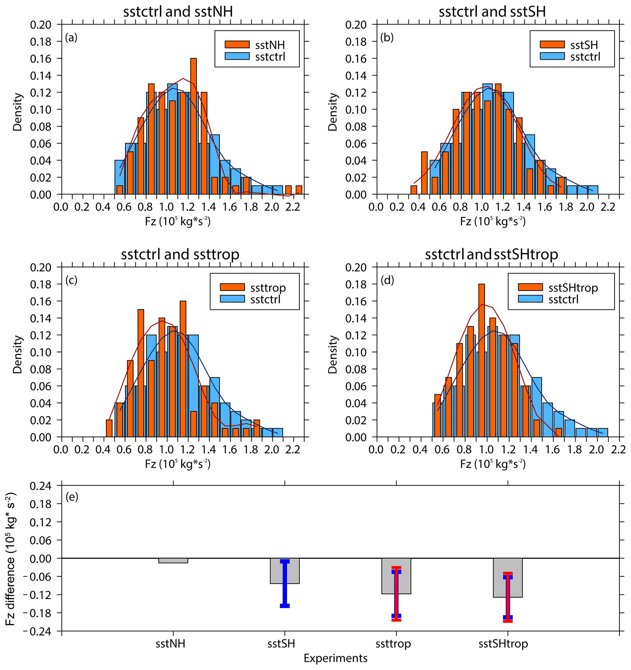
Figure 14 (a, b, c, d) Frequency distributions (pillars; blue for the control experiment and orange for sensitivity experiments) of vertical E–P flux (Fz; area weighted from 200 to 10 hPa over 70–50^∘ S) and its five-point low-pass filtered fitting curves (solid lines; blue for the control experiment and red for sensitivity experiments) derived from 100 ensemble members of the control experiment (sstctrl) and sensitivity experiments (a sstNH; b sstSH; c ssttrop; d sstSHtrop), respectively. (e) Mean differences (gray pillars) and corresponding uncertainties (error bars) of Fz between sensitivity experiments and the control experiment. The blue and red error bars reflect the 90 % and 95 % confidence levels calculated by two-tailed t test, respectively. The error bar is omitted when the significance of mean difference is lower than the corresponding confidence level.

Figure 15 (a) Trends of the southern hemispheric Brewer–Dobson circulation (arrows; units in horizontal and vertical components are 0.2 × 10⁻² and 0.2 × 10⁻⁴ m s⁻¹ yr⁻¹, respectively) and its stream function (shading) in September during (a) 1980–2000 and (b) 2000–2017 as derived from the MERRA-2 dataset. Data in 2002 are removed when trends are calculated in panel (b). (c) Differences in the Brewer–Dobson circulation (arrows; units in horizontal and vertical components are 10⁻² and 10⁻⁴ m s⁻¹, respectively) and its stream function (shading) between the O3ctrl and O3sen. (d, e, f) Differences in the Brewer–Dobson circulation and its stream function between the control experiment (sstctrl) and sensitivity experiments (d sstSH; e ssttrop; f sstSHtrop) with SST changes. The stippled regions represent the trends or differences in the stream function significant at/above the 90 % confidence level. The green contours from outside to inside (corresponding to p=0.1 and 0.05) represent the trends or differences in the vertical components significant at the 90 % and 95 % confidence levels, respectively.

In addition, the reanalysis datasets show that the Brewer–Dobson circulation related to wave activities in the stratosphere weakened significantly in early austral spring during 2000–2017 (Fig. 15b), which is contrary to the intensified trend during 1980–2000 (Fig. 15a). The transition of BDC around the year 2000 is believed to be associated with ozone depletion and recovery (e.g., Polvani et al., 2017, 2018). However, our modeling results suggest that the SST trend has been responsible for the weakening of BDC in September since the year 2000 (Fig. 15d, e, f), The response of BDC to ozone recovery is not significant (Fig. 15c) in September, especially for the branch near the Antarctic. These results indicate that, apart from the ozone depletion and recovery, the SST trend should also be taken into consideration when exploring the mechanism for the climate transition in the southern hemispheric stratosphere around the year 2000.

Previous studies reported that there is usually a time lag for tropic SST to affect extratropical circulation (e.g., Shaman and Tziperman, 2011). Thus, the impact of tropical SST change before September needs to be further examined. Our simulations indicate that the tropical SST trend in September plays a dominate role in weakening of stratospheric wave activity at the same month, and the effect of tropical SST change before September is negligible compared to that in September (detailed evidence to address this issue is shown in the Appendix).

7 Conclusions and discussions

This study has analyzed the trend of Antarctic stratospheric planetary wave activities in early austral spring since the early 2000s, based on various reanalysis datasets and model simulations. Using the change point method, we find that the Antarctic stratospheric wave activities in September have been weakening significantly since the year 2000, which means the intensified trend of wave activities noted in previous research (Hu and Fu, 2009; Lin et al., 2009) are reversed after the year 2000 in early austral spring. Further analysis suggests that the weakening of stratospheric wave activities is related to the weakening of tropospheric wave sources in extratropical Southern Hemisphere, which is mainly contributed by the wave 1 component.

As the Antarctic ozone also shows clear shift around the year 2000, we firstly examine the impact of ozone recovery on Antarctic stratospheric planetary wave activity. Our simulation results indicate that significant ozone recovery in the lower stratosphere changes the atmospheric state for wave propagation to some extent, inducing a slight decrease in the vertical wave flux over UTLS region in the subpolar Southern Hemisphere. Meanwhile, the changes in wave activity in the middle and upper stratosphere over the subpolar region induced by ozone recovery are not significant. Therefore, the ozone recovery has a minor contribution to the significant weakening of stratospheric planetary wave activity in September.

EOF analysis and correlation analysis indicate that the stratospheric wave activities in early austral spring during 2000–2017 are related to PC2 of SST over 20^∘ N–70^∘ S (i.e., the SHtrop region). The corresponding EOF2 mode also shows a good similarity to the spatial pattern of the SST trend, suggesting that the weakening of stratospheric wave activities is connected to the trend of SST in SHtrop region. Meanwhile, the link between the SST trend in NH region and the weakening of stratospheric wave activities is weak. The model simulations also support that the SST changes in SHtrop region lead to a weakening of tropospheric wave sources and stratospheric wave activities. The contribution of the SST trend in tropical region to the weakening of stratospheric wave activities is larger than that in the extratropical Southern Hemisphere. However, the response of tropospheric wave sources and stratospheric wave activities to SST trend in NH region is not significant. The contribution of the SST trend over the SHtrop region to the weakening of stratospheric wave activities is about 34 %. Finally, both reanalysis datasets and numerical simulations indicate that the Brewer–Dobson circulation related to stratospheric wave activity has also been weakening in early austral spring since the year 2000, which is also attributed to the changes in September SST in the tropics and extratropical Southern Hemisphere.

Although many researchers have claimed that the climate transition around the year 2000 in Southern Hemisphere is related to ozone depletion and recovery (e.g., Barnes et al., 2014; Banerjee et al., 2020), there is no contradiction between our results and these previous studies. First, the Southern Hemisphere tropospheric circulation (i.e., the SAM index, the tropospheric jet position, and the Hadley cell edge) shifts related to ozone changes in these previous studies basically occurred in austral summer (e.g., Son et al., 2008; Thompson et al., 2011; Barnes et al., 2014; Banerjee et al., 2020). These tropospheric circulation changes are induced by downward coupling of circulation anomalies in the stratosphere (e.g., Thompson et al., 2011) during October and November, when solar radiation covers the entire Antarctic and causes heating effects. However, the Antarctic stratospheric circulation response to ozone variation in September is not as strong as that in October or November (e.g., Thompson et al., 2011, Fig. 1b, d) because solar radiation can only reach part of Antarctic stratosphere during a majority period of September. This implies that the response of the atmospheric state in September to Antarctic stratospheric ozone change is not significant. Second, the FWSC component used in this study is an atmospheric module with prescribed SST and forcing gases. Therefore, our model results only indicate that the weakening of stratospheric wave activity can be attributed to SST changes, while the impact of ozone change in middle and low latitudes on SST cannot be determined based on these simulations. More efforts are needed to determine whether the trend transition signal of Antarctic stratospheric ozone can affect SST trends. This is an issue beyond the scope of this study, and further investigation is necessary by using a fully coupled Earth system model.

The Southern Hemisphere stratospheric wave activity trend from the early 1980s to the early 2000s has been investigated by Hu and Fu (2009; hereafter HF2009) and, hence, is not discussed in detail in the above. HF2009 attributed the strengthening of stratospheric wave activity in austral spring during 1979–2006 to the SST trends as well; however, they gave no more details about the trends of tropospheric wave sources. In this study, trends of tropospheric wave sources in September during 1980–2000 derived from MERRA-2 data are analyzed, and we also conducted an experiment (sstSHtrop) forced by the changes in September SST during 1980–2000 over 20^∘ N–70^∘ S (see Fig. S9 for applied SST anomalies). The model result indicates that the SST changes over 20^∘ N–70^∘ S contribute to intensification of wave 2 component of tropospheric wave sources (Fig. S10f) and weakening of the wave 1 component (Fig. S10e), which is overall analogous to the trends derived from MERRA-2 data (Fig. S10b, c). Accordingly, the simulated wave 2 component of the wave flux increases significantly in the stratosphere (Fig. S10h), while the response of the wave 1 component is not significant (Fig. S10i). In a word, the results from sstSHtrop80 suggest that the SST changes over 20^∘ N–70^∘ S induce a strengthening of stratospheric wave activity in September during 1980–2000. But it cannot explain the intensified wave 1 component of the stratospheric wave activity shown in Fig. 1b. A more detailed attribution of the trend of Antarctic stratospheric wave activity during 1980–2000 needs much more research.

The simulated stratospheric eddy heat flux (Fig. 11b in HF2009) forced by observed time-varying SST in HF2009 is relatively weak compared to that derived from reanalysis data (Fig. 6b in HF2009). Similarly, Wang and Waugh (2012; hereafter WW2012) used a stratosphere-resolving chemistry–climate model forced by time-varying factors to evaluate the trends of stratospheric temperature, residual circulation, and wave activity during recent decades, and the trend of cumulative eddy heat flux shown in their paper is not significant (Fig. 6 in WW2012). Additionally, Polvani et al. (2018) used time-varying ODSs that cover the period from the 1960s to the 2080s to simulate the Brewer–Dobson circulation and attained an obvious trend transition around the year 2000. We had also tried to conduct transient experiments forced by time-varying SST derived from ERSST v5 with different initial conditions; however, the trends of wave activities in the transient simulations are so weak, although the opposite trend signs exist during 1980–2000 and 2000–2018 (Table S2; Fig. S11). The significance of the simulated trend may be related to model performance and the length of simulating period. As the period we focus on is relatively short, and our purpose is attribution rather than generating a real trend, we perform the ensemble time slice experiments in this study, which are also used in many other previous researches (e.g., Hu et al., 2018; Kang et al., 2011; Zhang et al., 2016) to attribute trends in the atmosphere. In addition, most of the current climate models cannot generate a realistic wave activity trend, as waves in the atmosphere are linked with various processes and factors (e.g., Baldwin and Dunkerton, 2005; Garcia and Randel, 2008; Labitzke, 2005; Shindell et al., 1999; Shu et al., 2013; Xie et al., 2008).

Appendix A: Analysis of time lag for tropical SST affects Antarctic stratospheric wave activity

As stated in Sect. 2, the tropical SST anomalies (the linear increments) in the ssttrop experiment are also applied in July and August (Fig. S5a, b) to avoid abrupt SST variations from month to month, and the 2 months are taken as spin-up time. Therefore, whether the SST forcing in July and August also contributes to the weakening of Antarctic stratospheric wave activity in September or not cannot be justified based on the experiment ssttrop only. Here, we performed an additional experiment, ssttropAug, without September SST anomalies (Fig. S5f), to clarify whether the weakening of Antarctic stratospheric wave activity is induced by the tropical SST trend in the same month. Like other numerical experiments described in Table 1, the ssttropAug also includes 100 ensemble members that run from July to September and forced by the same initial conditions from the 21st year to the 120th year in July generated by free run. Detailed descriptions of ssttropAug and other relevant experiments in the paper are displayed in Table S1 in the Supplement for comparison. Figure S5 shows the applied global SST anomalies in ssttrop and ssttropAug from July to September.

The responses of tropospheric wave sources and stratospheric wave activities in ssttropAug are shown in Fig. S6a–c and d–f, respectively. Note that the anomalies of subpolar tropospheric geopotential height in September forced by changes in tropical SST in August does not superpose on their climatological patterns in an evident out-of-phase style (Fig. S6a–c). The anomaly of the wave 1 component of geopotential height shows a slight in-phase overlap with its climatology over subpolar region (Fig. S6b). Accordingly, the responses of stratospheric wave activities over the subpolar region of the Southern Hemisphere are not significant (Fig. S6d–f). The results here suggest that the decrease in the September vertical wave flux induced by SST changes in August is negligible when compared to the experiment with anomalous SST forcing in September (Fig. S6g), and the tropical SST trend in September plays a dominate role in the weakening of stratospheric wave activity in the same month.

Furthermore, we also use a linear barotropic model (LBM; e.g., Shaman and Tziperman, 2007, 2011) to quantify the timescale for the propagation of tropical anomalies to high latitudes. The LBM has been developed to solve the barotropic vorticity equation, which is given as Eq. (A1), as follows:

$$\begin{array}{}\text{(A1)}& {\displaystyle }\begin{array}{rl}\mathbf{J}(\overline{\mathit{\psi }},{\mathrm{\nabla }}^{\mathrm{2}}{\mathit{\psi }}^{\prime })& +\mathbf{J}({\mathit{\psi }}^{\prime },{\mathrm{\nabla }}^{\mathrm{2}}\overline{\mathit{\psi }}+f)+\mathit{\alpha }{\mathrm{\nabla }}^{\mathrm{2}}{\mathit{\psi }}^{\prime }\\ & +K{\mathrm{\nabla }}^{\mathrm{4}}{\mathrm{\nabla }}^{\mathrm{2}}{\mathit{\psi }}^{\prime }=R,\end{array}\end{array}$$

where the Jacobian J(A,B) is as follows:

$$\begin{array}{}\text{(A2)}& {\displaystyle }\mathbf{J}(A,B)={\displaystyle \frac{\mathrm{1}}{r^{\mathrm{2}}}}\left({\displaystyle \frac{\partial A}{\partial \mathit{\lambda }}}{\displaystyle \frac{\partial B}{\partial \mathit{\mu }}}-{\displaystyle \frac{\partial A}{\partial \mathit{\mu }}}{\displaystyle \frac{\partial B}{\partial \mathit{\lambda }}}\right),\end{array}$$

and the forcing function R is as follows:

$$\begin{array}{}\text{(A3)}& {\displaystyle }R=-\left(f+{\mathrm{\nabla }}^{\mathrm{2}}\overline{\mathit{\psi }}\right)D.\end{array}$$

ψ is the streamfunction, f is the Coriolis force, α is the Rayleigh coefficient, K is the diffusion coefficient, λ is the longitude, μ=sin (θ), θ is the latitude, r is the Earth's radius, and D is the divergence.

We use the wave 1 component of the stream function derived from the ensemble mean of sstctrl as the background field. In the LBM, the initial anomaly is given by the divergence. The divergence forcing field is limited to the range 40^∘ E–140^∘ W, 10^∘ S–0^∘ (Fig. S7) to ensure that the tropical initial anomaly of the stream function is superposed on its background field in an out-of-phase style. We set $D=-\mathrm{7.9}\times {\mathrm{10}}^{-\mathrm{7}}$ s⁻¹, which is the mean divergence over the forcing region. The LBM-simulated stream function anomalies are shown in Fig. S8b–i. Note that the anomalies in tropics only take a few days to arrive at the high latitudes in the Southern Hemisphere. After about 4 d, a stable anti-phase superposition of the stream function is well established in the extratropical Southern Hemisphere (Fig. S8f–i). These results are supported by previous studies (e.g., Shaman and Tziperman, 2011), which also indicate that the horizontal propagation of anomaly in atmosphere takes a few days.

Previous studies also reported that it takes about 4 d for wave 1 to propagate from the troposphere into the stratosphere and 1–2 d for wave 2 (e.g., Randel, 1987). Thus, the tropical oceans affect the stratosphere at mid–high latitudes with a lag of several days. However, the SST forcing field applied in CESM is on a monthly scale. It is reasonable to use the September SST trend to drive and explain the trends of extratropical circulation and wave activity in the same month.