the Creative Commons Attribution 4.0 License.
the Creative Commons Attribution 4.0 License.
 | 07 Dec 2022
Observation-based constraints on modeled aerosol surface area: implications for heterogeneous chemistry
Rachel A. Bergin
Monica Harkey
Alicia Hoffman
Richard H. Moore
Bruce Anderson
Andreas Beyersdorf
Luke Ziemba
Lee Thornhill
Edward Winstead
Tracey Holloway
Timothy H. Bertram
Heterogeneous reactions occurring at the surface of atmospheric aerosol particles regulate the production and lifetime of a wide array of atmospheric gases. Aerosol surface area plays a critical role in setting the rate of heterogeneous reactions in the atmosphere. Despite the central role of aerosol surface area, there are few assessments of the accuracy of aerosol surface area concentrations in regional and global models. In this study, we compare aerosol surface area concentrations in the EPA's Community Multiscale Air Quality (CMAQ) model with commensurate observations from the 2011 NASA flight-based DISCOVER-AQ (Deriving Information on Surface Conditions from COlumn and VERtically Resolved Observations Relevant to Air Quality) campaign. The study region includes the Baltimore and Washington, D.C. metropolitan area. Dry aerosol surface area was measured aboard the NASA P-3B aircraft using an ultra-high-sensitivity aerosol spectrometer (UHSAS). We show that modeled and measured dry aerosol surface area, Sa,mod and Sa,meas respectively, are modestly correlated (r2=0.52) and on average agree to within a factor of 2 () over the course of the 13 research flights. We show that does not depend strongly on photochemical age or the concentration of secondary biogenic aerosol, suggesting that the condensation of low-volatility gas-phase compounds does not strongly affect model–measurement agreement. In comparison, there is strong agreement between measured and modeled aerosol number concentration (, r2=0.63). The persistent underestimate of Sa in the model, combined with strong agreement in modeled and measured aerosol number concentrations, suggests that model representation of the size distribution of primary emissions or secondary aerosol formed at the early stages of oxidation may contribute to the observed differences.
For reactions occurring on small particles, the rate of heterogeneous reactions is a linear function of both Sa and the reactive uptake coefficient (γ). To assess the importance of uncertainty in modeled Sa for the representation of heterogeneous reactions in models, we compare both the mean and the variance in to those in γ(N2O5)(N2O5)meas. We find that the uncertainty in model representation of heterogeneous reactions is primarily driven by uncertainty in the parametrization of reactive uptake coefficients, although the discrepancy between Sa,mod and Sa,meas is not insignificant. Our analysis suggests that model improvements to aerosol surface area concentrations, in addition to more accurate parameterizations of heterogeneous kinetics, will advance the representation of heterogeneous chemistry in regional models.
- Article
(5991 KB) - Full-text XML
-
Supplement
(380 KB) - BibTeX
- EndNote


1.1 The role of aerosol surface area in heterogeneous reaction kinetics
Reactions occurring at atmospheric interfaces, such as suspended aerosol particles, catalyze the production and loss of key gas-phase compounds in Earth's atmosphere with important implications for regional air quality (Chang et al., 2011). The rate of heterogeneous reactions occurring at the surface of aerosol particles is a function of the gas–aerosol collision frequency and the reaction probability per collision. Variability in gas–aerosol collision frequency is determined by the aerosol surface area concentration. The probability of reaction, or the net reactive uptake coefficient (γ), is reaction specific and dependent on chemical kinetics, gas accommodation at the surface, and near-surface diffusion (Abbatt et al., 2012). Collectively, the first-order removal rate of a gas-phase species (A) from the atmosphere can be written as
where the heterogeneous reaction rate constant (khet), in the absence of gas-phase diffusion limitations, can be written as
where ω is the mean molecular speed of the gas-phase molecule (m s−1), and Sa is the surface area concentration of aerosol particles (m2 m−3).
To date, most evaluations of the role of heterogeneous chemistry on gas-phase composition have focused on uncertainty in parameterizations of reactive uptake coefficients, such as the reactive uptake of dinitrogen pentoxide (N2O5) due to its role as a NOx sink (Brown et al., 2009; Evans and Jacob, 2005; MacIntyre and Evans, 2010; McDuffie et al., 2018). In comparison, there has been less focus on model representation of aerosol surface area concentrations, despite the fact that khet is linearly dependent on Sa. An accurate representation of aerosol surface area in regional and global chemical transport models is challenging, as Sa is a complex function of size-dependent aerosol particle emissions, chemical transformations, and removal processes. Here, we directly compare aerosol surface area concentrations in a regional chemical transport model with commensurate aircraft measurements to assess the representation of Sa in regional air quality models.
1.2 Calculation of aerosol surface area in regional air quality models
The total aerosol particle surface area concentration has been calculated in air quality models using a variety of approaches, including the discrete representation of the particle size distribution in defined size ranges, known as the sectional method (Adams and Seinfeld, 2002; Gelbard et al., 1980; Jacobson, 2001; Lee et al., 2009; Lee and Adams, 2012; Luo and Yu, 2011; Spracklen et al., 2006; Trivitayanurak et al., 2008; Yu and Luo, 2009), and a continuous modal representation of the particle size distribution (Kleeman et al., 1997; Mann et al., 2010; Meng, 1998; Pringle et al., 2010; Sartelet et al., 2006; Stier et al., 2005; Vignati et al., 2004; Zhang et al., 2010a). Here, we review the modal representation of particle size distributions implemented in the Community Multiscale Air Quality (CMAQ) model and the calculation of both wet and dry total aerosol surface area (Sa). Aerosol particle size distributions in CMAQ follow the method developed for the Regional Particulate Model, an extension of the Regional Acid Deposition Model (Binkowski, 1999; Binkowski and Roselle, 2003), where the total particle size distribution is treated as the superposition of three separate lognormal distributions (or modes) – Aitken, accumulation, and coarse modes (Binkowski, 1999; Whitby, 1978). The lognormal particle size distribution for each mode is defined as
where N is the total number concentration, D is the particle diameter, and Dg and σg are the geometric mean diameter and geometric standard deviation. Under this definition, the Aitken mode describes aerosol particles of diameter smaller than approximately 0.1 µm with a median diameter of 0.03 µm, while the accumulation mode encompasses the diameter range of 0.1 to 2.5 µm with a median diameter of 0.3 µm (Binkowski, 1999). The coarse mode describes particles of diameter 0.3 to about 10 µm, with a median diameter of 6 µm. It should be noted that there is uncertainty in the exact size distributions within CMAQ, dependent on emissions parameters, so the median diameters within modes are approximate (Elleman and Covert, 2010). Particle nucleation and growth result in changes to the mode diameter and can result in the transfer of particle number, surface area, and mass to the next larger size (e.g., Aitken to accumulation). Outside of particle growth and nucleation, the approximate median diameters are unchanged. The size ranges for each mode are based on Whitby (1978), and geometric standard deviation is also based on Whitby (1978) but has been updated to the geometric standard deviations from Elleman and Covert (2010).
Three integral properties of the aerosol size distribution are calculated in CMAQ, the zeroth (M0), second (M2), and third moments (M3), where the kth moment of the size distribution is calculated as
In this representation, N=M0, Sa=πM2, and , where V is the total aerosol volume (Binkowski, 1999; Binkowski and Roselle, 2003). Though M2 is utilized in CMAQ's aerosol subroutines, it is multiplied by π prior to use in main CMAQ routines, such that it is identified as a modal surface area (Binkowski and Roselle, 2003).
The time rate of change of each moment is calculated for each grid box and time interval as
where P and L represent the production and loss of Mk in each aerosol mode. With respect to Sa (Sa=πM2), neglecting transport terms, P2 includes new particle formation (Aitken mode only), condensational growth, and primary emissions, and L2 includes intramodal coagulation and dry and wet deposition. Primary aerosol emission rates are sourced from the 2011 EPA National Emissions Inventory, which characterizes emissions based on source type and location. Within CMAQ, all primary aerosol emissions, independent of source type, are parameterized with modal size distributions per Elleman and Covert (2010) (see the Supplement). In the version of CMAQ used here, new particle formation is based on classical, binary homogeneous nucleation (Kulmala et al., 1998). Particle growth is described by Binkowski and Roselle (2003) and secondary organic aerosol (SOA) schemes in Carlton et al. (2010).
In the interpretation of model Sa, the following model-specific details should be considered: (1) fine particles (Aitken and accumulation modes) do not coagulate with coarse-mode particles, and coarse-mode particles do not coagulate with each other (Binkowski and Roselle, 2003). (2) The size distribution for primary PM2.5 emissions is assumed to have a geometric mean (Dg=0.3 µm) and geometric standard deviation (σg=2), and >99 % of PM2.5 emissions are assigned to the accumulation mode (Binkowski and Roselle, 2003), which may have consequent effects on the aerosol surface area distribution. (3) Particles are assumed to be spherical.
The condensation of water is accounted for in the chemical evolution of M2; thus M2 is inherently the wet second moment (), which is used in the calculation of heterogeneous chemical reactions. In addition to , a dry second moment () is calculated as a function of the third moment (M3) as
In the following analyses, we concentrate on the comparison of modeled and measured Sa to evaluate the relative uncertainty associated with model descriptions of heterogeneous kinetic mechanisms (i.e., reactive uptake coefficients, γ) and aerosol particle size distributions (i.e., aerosol surface area, Sa) that, combined, dictate the fate of reactive gas-phase molecules.
1.3 Previous model–measurement comparisons of aerosol surface area
Evaluation of regional air quality models has largely focused on criteria air pollutants such as ozone (O3) and particle mass (e.g., PM2.5) (Appel et al., 2021). Previous model evaluation of particle mass has focused on an array of metrics including mass concentration (Gantt et al., 2012; Spak and Holloway, 2009; Wang et al., 2009), number concentration (Park et al., 2006; Ranjithkumar et al., 2021; Wang et al., 2009; Zhang et al., 2010b), size distribution (Kelly et al., 2011; Nolte et al., 2015; Park et al., 2006; Zhang et al., 2010b), composition (Knote et al., 2011; Nolte et al., 2015; Prank et al., 2016), and aerosol optical depth (Ghan et al., 2001; Knote et al., 2011). There has been a very long and detailed history of CMAQ evaluation of PM2.5, including ground-based (Baker et al., 2018; Fan et al., 2005; Ghim et al., 2017; Hogrefe et al., 2009, 2015; Liu and Zhang, 2011; Prank et al., 2016; Smyth et al., 2006; Wang et al., 2021; Yu et al., 2012, 2008b, 2008a; Zhang et al., 2019, 2006, 2010c), ship-based (Yu et al., 2012), and aircraft-based measurements (Baker et al., 2018; Chen et al., 2020; Yu et al., 2012). For 15 studies comparing ground-based measurements of PM2.5 to CMAQ outputs between 1999 and 2018, 10 saw an underestimation of PM2.5 by the model ranging between 6 % –75 % (Ghim et al., 2017; Liu and Zhang, 2011; Prank et al., 2016; Wang et al., 2021; Yu et al., 2008a, 2012, 2008b; Zhang et al., 2019, 2006, 2010c), dependent on pollution events and rural versus urban location, while 4 found that CMAQ predicted observations well (Baker et al., 2018; Fan et al., 2005; Hogrefe et al., 2009; Smyth et al., 2006), matching general trends in the observational data, and 1 saw an overestimation of observational data (Hogrefe et al., 2015). Of the three aircraft studies, two saw significant underestimation of PM2.5 aloft (Baker et al., 2018; Chen et al., 2020), while one saw overestimation in some PM2.5 compositional components and underestimation in others (Yu et al., 2012).
Particle surface area specifically is not regulated as a criteria air pollutant as standards of measurement and air quality controls are determined on a mass per unit volume basis. However, particle surface area indirectly affects the concentration of PM2.5 and O3 as it can serve to regulate the lifetime of nitrogen oxides (Chang et al., 2011; Geyer and Stutz, 2004; Portmann et al., 1996; Stadtler et al., 2018) and hydrogen oxides (George et al., 2013; Lakey et al., 2015; Martin et al., 2003; Thornton et al., 2008; Thornton and Abbatt, 2005), the production rate of secondary organic aerosol (Gaston et al., 2014), and new particle formation and growth rates, as the preexisting aerosol surface area serves as a condensation sink for low-volatility gas-phase compounds (Donahue et al., 2014; Trump et al., 2014). There are few reports of model–measurement comparisons of particle surface area, and those that have been reported in the literature have focused on comparisons of heavily spatially and temporally averaged concentrations (e.g., field campaign averages). For example, Simon et al. (2010) compared ground-based aerosol surface area concentrations calculated in the CAMx model to measurements made aboard the RV Ronald H. Brown in the Gulf of Mexico and the Houston Ship Channel with two differential mobility particle sizers and an aerodynamic particle sizer (Bates et al., 2008). The results of these studies are given in Table 1. Model prediction of median Sa in the Gulf of Mexico was similar to the measurement data (), with median values and ranges again shown in Table 1. In comparison, model prediction of median Sa in the Houston Ship Channel, where there is large spatial and temporal fluctuation in Sa relative to the smaller interquartile range seen in the Gulf of Mexico, yielded . Modeled Sa was also compared to measured Sa aloft on two research flights from the TexAQS II/GoMACCS field study in September and October 2006. The range of measured Sa values (<600 µm2 cm−3) matched well with the average values predicted in the CAMx model, though the maximum modeled values were much larger than those measured (4000–8000 µm2 cm−3 compared to <600 µm2 cm−3), consistent with the RV Ronald H. Brown comparisons. Overall, it should be noted that on a regional scale, modeled values agree well with measurements of aerosol Sa; however maximum modeled values were larger than those measured both for ground-based measurements and those aloft.
Table 1Comparison of model and measured aerosol surface area concentrations. Simon et al. (2010) compared CAMx model results with ground-based measurements in the Gulf of Mexico and the Houston Ship Channel. Jaeglé et al. (2018) compared measurements from the WINTER campaign and GEOS-Chem modeled data at the surface and aloft between 3.5 and 4.5 km.
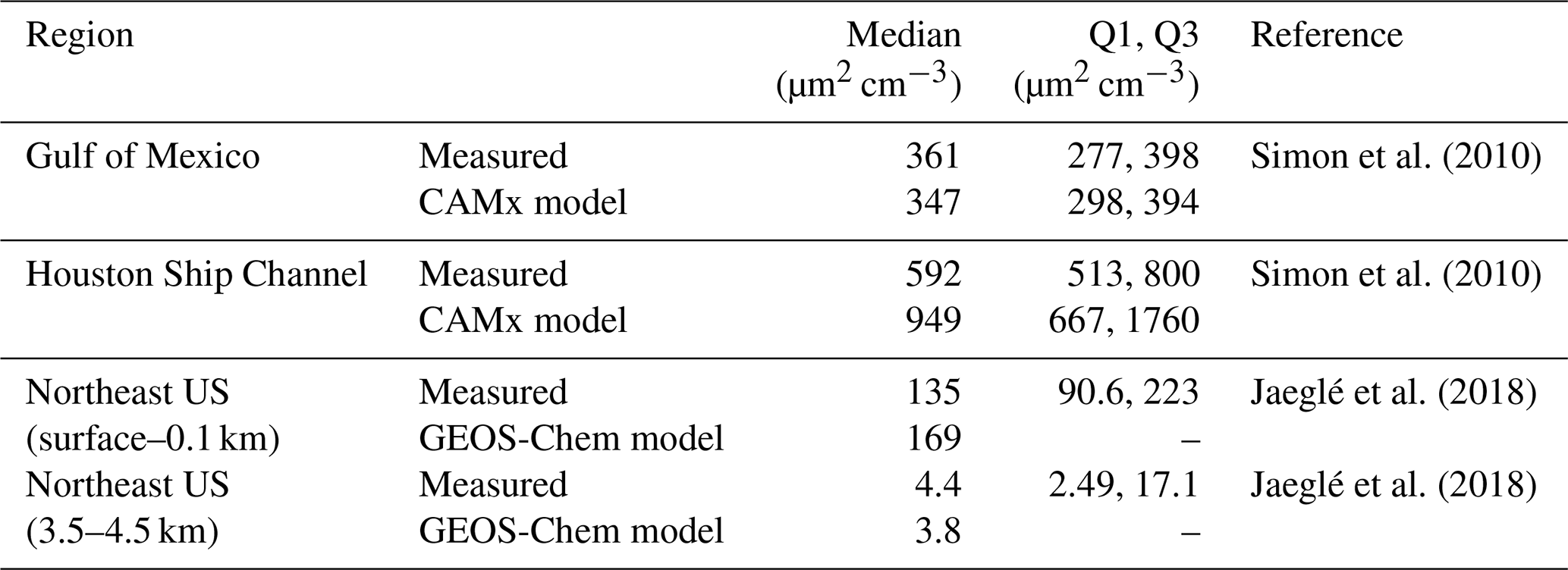
More recently, modeled dry surface area concentrations were assessed over the northeast US during the 2015 Wintertime INvestigation of Transport, Emissions, and Reactivity (WINTER) aircraft campaign (Jaeglé et al., 2018). While quantitative assessment of aerosol surface area was not the focus of this study, dry aerosol Sa was calculated by combining dry aerosol size distribution observations from a passive cavity aerosol spectrometer probe and ultra-high-sensitivity aerosol spectrometer and comparing these to the GEOS-Chem chemical transport model. Two versions of the model, a reference and improved model, were compared to the observations within 13 altitude bins, ranging from surface to 4.5 km; here we focus on the improved model results. The GEOS-Chem model medians were encompassed by the observed interquartile ranges in each altitude bin. The improved model showed excellent agreement with measurements when compiled over large spatial and temporal scales, where was 1.25 and 0.68 for the surface and 4.5 km comparisons, respectively.
Given the importance of accurate model representation of aerosol surface area to multiple atmospheric processes, and the limited number of prior studies conducted in urban environments, we revisit this comparison using a regional air quality model aerosol and commensurate aircraft observations conducted in an urban environment.
2.1 Aerosol evaluation in the CMAQ model
CMAQ simulations were performed as described by Abel et al. (2018, 2019) and Harkey et al. (2021), with carbon bond 5 chemistry, anthropogenic emissions from the 2011 National Emissions Inventory, and input meteorology from the Weather Research and Forecasting (WRF) version 3.2.1 (Skamarock et al., 2008), constrained to the North American Regional Reanalysis (NARR; Messinger et al., 2006; Abel et al., 2018, 2019; Harkey et al., 2021). The CMAQ simulation utilized here employed CMAQ version 5.2.1 (Byun and Schere, 2006; Nolte et al., 2015) and was run with 25 vertical layers from the surface to 100 hPa, a 12×12 km grid, and hourly temporal resolution. Anthropogenic emissions and emissions from fires (both prescribed and not) were based on the 2011 National Emissions Inventory version 2, with in-line estimates of NO and NO2 produced by lightning, boundary conditions from the Model for Ozone and Related Chemical Tracers version 4 (MOZART; Emmons et al., 2010), and biogenic emissions from WRF output in the Model of Emissions of Gases and Aerosols from Nature version 2.1 (MEGAN; Guenther et al., 2012). The model was run from 20 May through 31 August 2011, to include 11 d of spin-up (Harkey et al., 2021). The dataset utilized in this analysis is only a subset of the model dataset originally run at UW-Madison.
CMAQ was also run for the time period of the 2015 WINTER field campaign for comparison of modeled and measured N2O5 uptake coefficients. This CMAQ simulation also employs input meteorology constrained to NARR, calculated using WRF version 3.8.1 (Skamarock et al., 2008). Anthropogenic emissions were taken from the 2016 National Emissions Inventory Collaborative, version 1 (NEIC, 2019). Emissions from fires and boundary conditions were taken from the EPA Air QUAlity TimE Series (EQUATES) project (https://www.epa.gov/cmaq/equates, last access: 29 November 2021). Biogenic emissions and lightning NOx emissions were both calculated in-line. This simulation employed CMAQ version 5.3.2 (Appel et al., 2021), with carbon bond 6 chemistry (Emery et al., 2015; Luecken et al., 2019). The WINTER period simulation was run from 21 January through 16 March 2015, to include 11 d of spin-up, with hourly output on a 12×12 km grid and on 35 vertical levels from the surface to 100 hPa.
The CMAQ simulation for the 2011 DISCOVER-AQ (Deriving Information on Surface Conditions from COlumn and VERtically Resolved Observations Relevant to Air Quality) period employed the “AERO6” aerosol module (Binkowski and Roselle, 2003; Carlton et al., 2010; Foley et al., 2010; Sonntag et al., 2014), where primary and secondary aerosols are characterized by bimodal lognormal size distributions, and the total size distribution is the sum of three aerosol size modes, Aitken, accumulation, and coarse modes, with median diameters of 0.03, 0.3, and 6 µm respectively. The CMAQ simulation for the 2015 WINTER period employed the “AERO7” aerosol module, which builds on the AERO6 module, with updates to aerosols formed by monoterpene oxidation, anthropogenic volatile organic compounds (VOCs), and aerosol liquid water (Pye et al., 2015, 2017; Qin et al., 2021; Xu et al., 2018). The CMAQ simulation for the DISCOVER-AQ period employed the default heterogeneous N2O5 uptake (Davis et al., 2008), while the simulation covering the WINTER period employed a N2O5 uptake modified per Bertram and Thornton (2009).
Due to the modality of the CMAQ representation of aerosols, we calculate each parameter relating to the aerosol dataset separately for each mode, and these are then combined to result in a total value that can be directly compared to the DISCOVER-AQ observational data. The total CMAQ dry surface area is computed as the sum of the modal dry surface areas. The variable SRF is an output of CMAQ but is defined as SRF . SRF is a modal variable like each moment, such that total surface area = SRFATKN + SRFACC + SRFCOR (dry surface area in the Aitken, accumulation, and coarse modes, respectively).
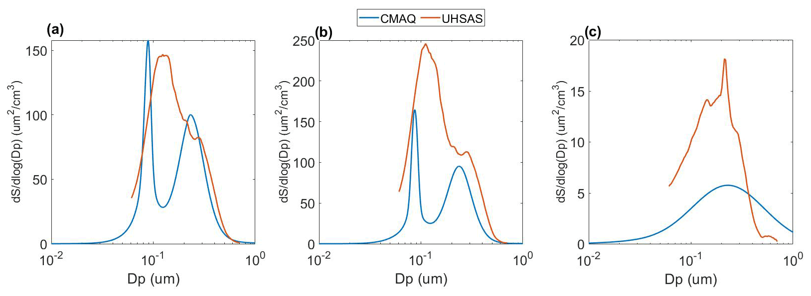
Figure 1Modeled (blue) and measured (orange) dry aerosol surface area distributions averaged over the DISCOVER-AQ sampling domain of Baltimore and Washington, D.C. at (a) all altitudes, (b) altitudes below 1 km, and (c) altitudes above 3 km for 1 July 2011.
2.2 DISCOVER-AQ 2011 campaign
Research flights conducted during the NASA DISCOVER-AQ campaigns were designed to measure the vertical and spatial distribution of key air pollutants in urban environments, with a focus on connecting surface measurements with vertically integrating satellite observations. The first DISCOVER-AQ campaign, conducted aboard the NASA P-3B aircraft during July 2011, was comprised of 14 science flights in the Baltimore and Washington, D.C. area (Crawford et al., 2014; Crawford and Pickering, 2014; NASA, 2012). The 2011 DISCOVER-AQ campaign was the first of a series of flights with an objective of narrowing the gap of satellite and observational data and air quality utilizing near-surface air pollution measurements. Science flights concentrated on high-time-resolution measurements of atmospheric composition in the convective boundary layer. Here, we focus on measurements of dry aerosol surface area concentration (Sa), determined from high-time-resolution (1 Hz) size distributions made using an ultra-high-sensitivity aerosol spectrometer (Droplet Measurement Technologies, UHSAS) integrating between 60<dp<1000 nm, which captures the peak of the surface area distribution, shown in Fig. 1 below. The UHSAS measures the particle size from optical light scattering, which was calibrated during DISCOVER-AQ using NIST-traceable polystyrene latex spheres whose refractive index may differ slightly from that of real-world aerosols that may result in a slight under-sizing bias (Moore et al., 2021). Ambient air was sampled through an isokinetic inlet, allowing the aerosol temperature to quickly equilibrate to that of the cabin of the P3-B aircraft. Along with additional ram pressure heating in the inlet during flow deceleration, particles reach an RH of below 40 %–50 %, meaning the aerosol is considered to be dry. The term “dry” here distinguishes that the particle hydration state is greatly reduced compared to that of the unperturbed ambient air. It is important to note that aerosol water is not accounted for in the following model–measurement comparison, though there would be some aerosol water present at the higher end of the 40 %–50 % RH threshold, which may impact the comparison of the measured aerosol to dry aerosol in the model. The particle mobility size from 10–310 nm diameters was measured with a TSI scanning mobility particle sizer (SMPS) with 45 s time resolution, and the particle aerodynamic size from 500–4000 nm diameters was measured with a TSI aerodynamic particle sizer (APS) at 1 Hz. On the representative day shown in Fig. 1, SMPS data showed that approximately 5.8 % of the surface area fell below the 60 nm threshold of the UHSAS measurement for an average surface area distribution for the average of all altitudes, while the APS indicated that supermicron particles did not contribute to the particle surface area. The distribution comparison between the model and measurement differs in shape at different altitudes. Figure 1b shows a comparison of the near-surface data, below 1 km, which gives a very similar distribution to that of the average of all altitudes. However, Fig. 1c, or that above 3 km altitude, shows a different shape and one that is more comparable between model and measurement. It should be noted that the axis scales in Fig. 1b and c do not match, showing a discrepancy in distribution calculation between CMAQ and DISCOVER-AQ that will be discussed in later sections. For simplicity, we choose to focus exclusively on the UHSAS size distribution data given their high frequency and wide size range of particle diameter, but it is important to note that not all of the particle surface area is captured by the UHSAS instrument. UHSAS data are available to the public at the NASA Langley Atmospheric Science's Data Center and Distributed Active Archive Center (https://doi.org/10.5067/Aircraft/DISCOVER-AQ/Aerosol-TraceGas). In the following analysis we utilize observations of nitric oxide (NO) and nitrogen dioxide (NO2) measured with the NCAR four-channel chemiluminescence instrument (Ridley and Grahek, 1990) and carbon monoxide (CO) measured via differential absorption CO measurement (DACOM) (Sachse et al., 1987) to assess differences in modeled and measured aerosol surface area.
2.3 Model–measurement comparison
To compare measured and modeled Sa, we sample the hourly 12 km × 12 km CMAQ output at the time and location of each DISCOVER-AQ sampling point. The spatial resolution of CMAQ, relative to the DISCOVER-AQ flight, is shown in Fig. 2 for the 28 July 2011 research flight, where the color corresponds to the modeled surface-level dry Sa (in µm2 cm−3) at noon EST. Indexing and analysis of the two aforementioned datasets was completed in MATLAB. Each 1 s data point from the DISCOVER-AQ 2011 campaign was mapped to the nearest (as described below) 4D index (time of day, latitude, longitude, and altitude) in the lower time and spatial resolution CMAQ model for direct comparison. The nearest 1 h averaged CMAQ time point was selected based on the time window that encompassed the aircraft flight time; i.e., a flight time of 09:16:00 was mapped to CMAQ time period of 09:00–09:59. The nearest 12 km × 12 km CMAQ grid box was also selected based on the grid box that encompassed the aircraft location at the time of sampling. The nearest CMAQ altitude (or layer) was identified by locating the aircraft height within one of the 25 indexes in which the altitude was encompassed. With all four CMAQ indexes assigned to each data point, the 1 s DISCOVER-AQ dataset could be fully mapped and compared to that from the CMAQ model. It should be noted that there are far more data points in the observed data than in the model due to resolution constraints, and thus the model is being oversampled. Each of the four indexes were concatenated together in the order defined in CMAQ, namely latitude, longitude, layer (altitude), and time. This process was utilized for each data point for an entire flight of DISCOVER-AQ and was then replicated for each subsequent flight. The result of this approach is shown in Fig. 3, for the comparison of modeled and measured carbon monoxide (CO). The coefficient of determination (r2) for the linear regression of modeled vs measured CO concentration (COmod COmeas) was 0.44 with a slope of 1.0499±0.0007. The large variance highlights the spatial and temporal mismatch of model sampling and measurement, while the near-unit correlation coefficient indicates that on average modeled and measured CO agree. This agreement implies that the model–measurement comparison of many well-understood parameters should be accurate and that there is not a fundamental issue in comparing modeled and measured data between the two datasets.

Figure 2Map of the Baltimore–Washington D.C. area representative of the July 2011 DISCOVER-AQ flights with an example flight path from 28 July 2011. The flight path is overlaid on the CMAQ model grid, showing the modeled surface area in each 12 km × 12 km grid box at noon EST (16:00 UTC).
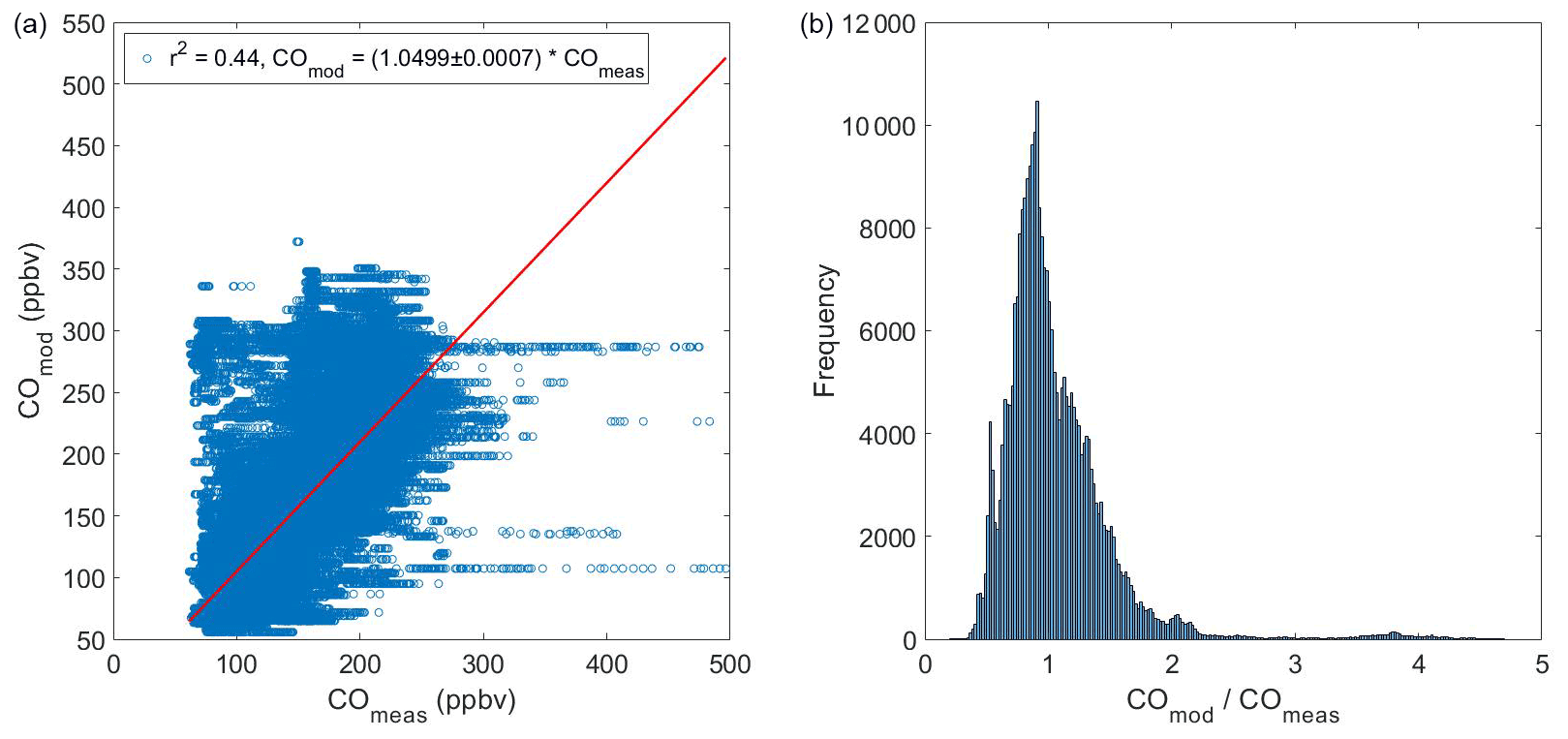
Figure 3(a) Linear regression of modeled vs measured carbon monoxide (CO) mixing ratio (in ppbv) and (b) histogram of the ratio of modeled-to-measured CO over the full DISCOVER-AQ campaign.
3.1 Campaign-averaged comparison of aerosol surface area concentrations
First, we assess general agreement between campaign-averaged modeled and measured surface area concentrations. The observational data are from the 13 DISCOVER-AQ flights during July 2011 (1–29 July). The final research flight consisted of a dual highway leg conducted south along the Baltimore–Washington Parkway and north along I-95 at low altitude to compare the two roadways. Given the proximity to a large point source, this research flight was not included in the following analysis. The observational data from the UHSAS included number, surface area, and volume measurements, though the focus of this study is primarily surface area (Sa).
In this analysis, we compare dry surface area concentrations as the DISCOVER-AQ measurements were made at an RH below 40 %–50 % and are thus considered dry, and we do not have direct measurements of particle growth factors for comparison of wet Sa. However, it is important to note that Sa used in E2 is the surface area concentration at ambient humidity, and any uncertainty in modeled aerosol hygroscopicity will propagate to the aerosol surface area concentration used in E2. Figure 4 shows the campaign-averaged vertical profile of both the measured dry UHSAS surface area (Sa,meas) and the modeled dry CMAQ surface area (Sa,mod), along with the interquartile ranges separated into 1 km altitude bins. Since the UHSAS measurement frequency is 1 Hz, the CMAQ modeled data are at 1 h time resolution, and the model samples a full domain in 12 km grid boxes compared to the smaller domain sampled by aircraft, there are many more measurement data points (N=330 204) than comparable modeled data points (N=5196) over the course of the flight campaign. In Fig. 4, the UHSAS measurements have been averaged to the spatial and temporal resolution of the model, such that the number of observational points is the same as the number of model points. The light gray error bars shown in Fig. 4a reflect the standard deviation of the data from the mean at that point in time and space. It should be noted that the error bars on this dataset are large, due to the spatial and temporal mismatch between model and measurement in a highly heterogeneous sampling domain. For both model and measurement, the surface area increases towards the surface, as is to be expected, and decreases with altitude. The vertical profile is well captured by the CMAQ model; however, there is a larger range of measured surface area concentrations than is seen in the corresponding model altitude bin.
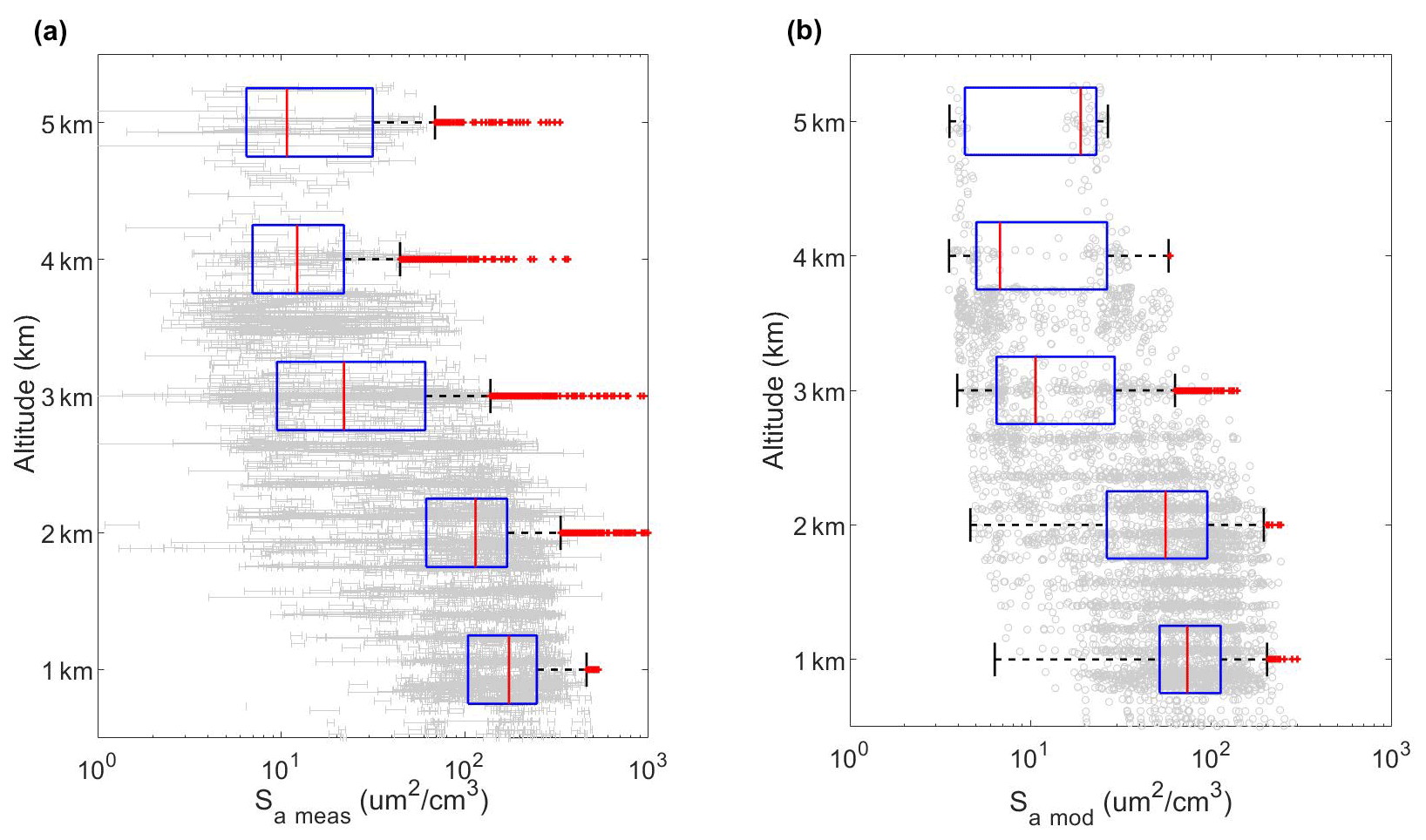
Figure 4Average vertical profile of (a) measured DISCOVER-AQ aerosol surface area concentration (Sa,meas) and (b) CMAQ aerosol surface area concentration (Sa,mod) over the entirety of the DISCOVER-AQ campaign. Each measured point is an average of the points included in that 4D index corresponding to CMAQ. The overlaid box plots show the median (red line within blue box) and interquartile ranges (blue box with the 25th percentile at the left end and 75th percentile at the right end) in 1 km altitude bins. The labels on the altitude axis lie at the midpoint of the 1 km altitude bin, and red crosses indicate outliers from the majority of the dataset at that altitude portion.
As shown in Fig. 4, measured Sa is on average larger than modeled Sa, particularly at low altitude, where the ratio of the median, modeled Sa to measured Sa near the surface (z<1 km) is 0.47. This contrasts with what has been reported previously in the literature. For example, both Jaeglé et al (2018) and Simon et al. (2010) found that the median modeled near-surface Sa was consistently larger than measured Sa ( 1.04–1.6).
The comparison between modeled and measured Sa is also shown with histograms in Fig. 5 for all altitudes (5a, b) and for the surface-level measurements (0–1 km; 5c, d). While the number of points is not consistent between the model and measurement datasets due to the 12 km grid box constraint and time frequency in CMAQ, differences in the range in surface area concentrations are observed. Measured surface area concentrations range between 0–1.87×103 µm2 cm−3, with the vast majority of data below 420 µm2 cm−3, while modeled Sa ranges between 0–300 µm2 cm−3.
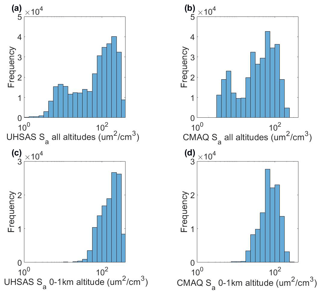
Figure 5Histograms of (a) measured aerosol surface area concentration (DISCOVER-AQ) at all altitudes, (b) modeled aerosol surface area concentration (CMAQ) at all altitudes, (c) measured aerosol surface area in the 0 to 1 km altitude bin, and (d) modeled aerosol surface area in the 0 to 1 km altitude bin over the entirety of the DISCOVER-AQ campaign.
3.2 Direct model–measurement comparison
A linear regression of CMAQ modeled dry aerosol surface area concentration and measured aerosol surface area concentration is shown in Fig. 6. The measured data have been averaged to the space and time domain of CMAQ (latitude, longitude, altitude, and time). The coefficient of determination (r2) for the linear regression of modeled and measured Sa was 0.52 with a slope of 0.437±0.004, indicating that the measured Sa is on average twice that of the model value.
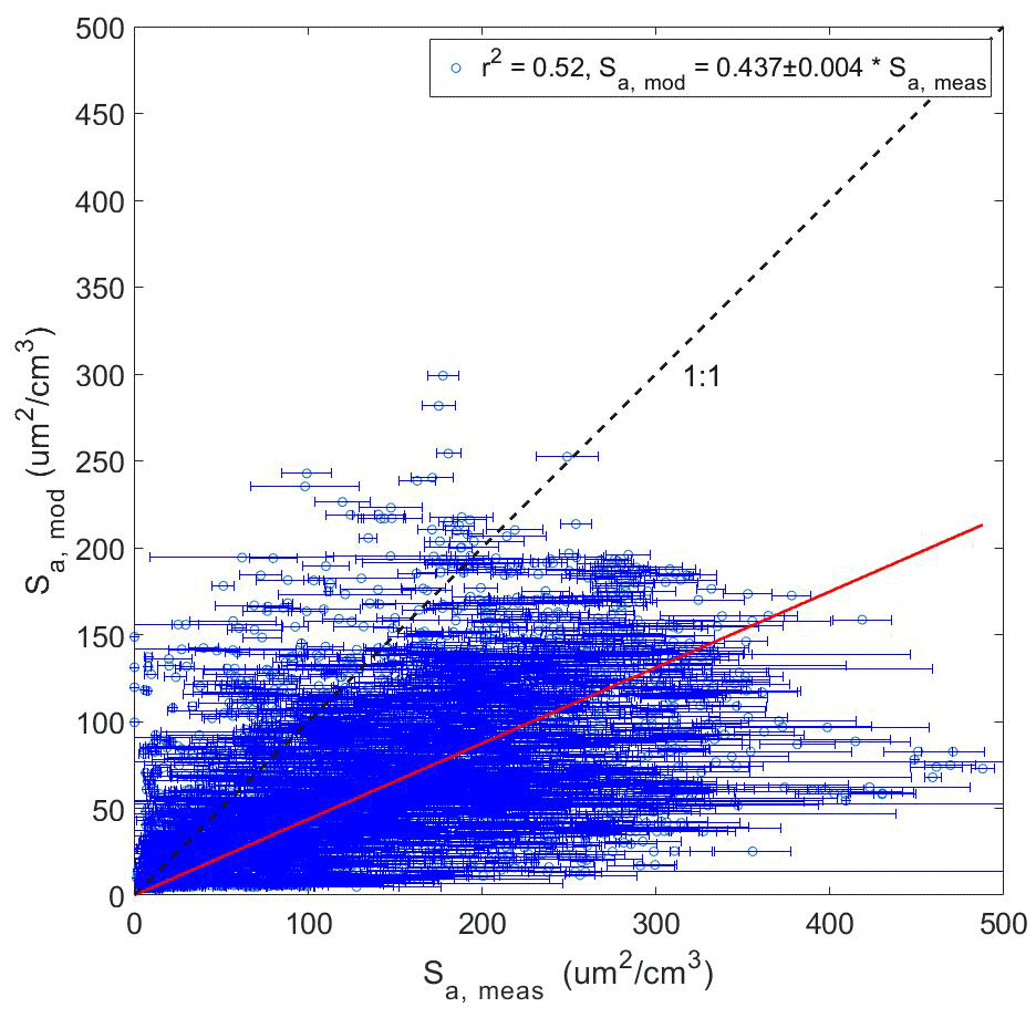
Figure 6Comparison of Sa,mod and Sa,meas over the full DISCOVER-AQ campaign with measurement data averaged to the corresponding model latitude, longitude, altitude, and time point.
The histogram of the surface area ratio () throughout the campaign in Fig. 7 shows that the model underpredicts the measured surface area ratio in 81 % of the comparison points. The model underpredicts Sa by a factor of 2 44 % of the time. In the following section, we explore potential causes for model–measurement disagreement, including model–measurement spatial and temporal differences, the spatial distribution of primary emissions, and/or treatment of secondary aerosol formation.
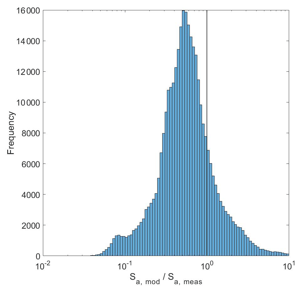
Figure 7Histogram of the ratio of modeled-to-measured aerosol surface area concentration () over the full DISCOVER-AQ campaign.
In the following section, we explore the source of model–measurement discrepancy in Sa discussed in Sect. 3. We begin by investigating the dependence of on altitude and proximity to primary aerosol sources. We then investigate the role of temporal and spatial resolution as CMAQ has a much coarser resolution, both spatially and temporally, than the measured data. Finally, we investigate the possibility of impacts on from anthropogenic and biogenic indicators as they are tied to aerosol emissions. It is also important to acknowledge that some of the model–measurement disagreement could be due to processes not considered in the model such as phase separation, viscosity changes of aerosols, and direct modeling of clouds impacting cloud processing of aerosols, though the impacts of these processes are not investigated further in this work. The lack of a fourth mode below the Aitken mode for nucleation of particles and growth to the Aitken mode also impacts the accuracy of the size distribution within CMAQ and may explain a portion of the model–measurement disagreement, though it is known that improving the default parameterization does not reduce all errors to the size distribution (Elleman and Covert, 2009b).
4.1 Dependence of on altitude
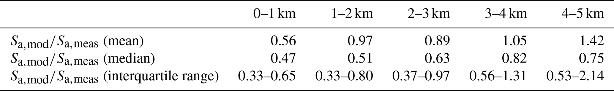
Given the strong dependence of Sa on altitude as shown in Fig. 4, we first explore if part of the variance in shown in Fig. 6 can be explained by altitude. In Fig. 8, we show as a function of altitude. As shown, there is an altitude dependence in , where the mean, median, and interquartile range (25th to 75th percentile) are given in Table 2 for the 1 km altitude bins from 0–5 km. Model–measurement discrepancy in Sa is largest at low altitude, where particle number concentrations are highest, proximity to particle sources is close, and heterogeneity in particle number concentrations is largest.
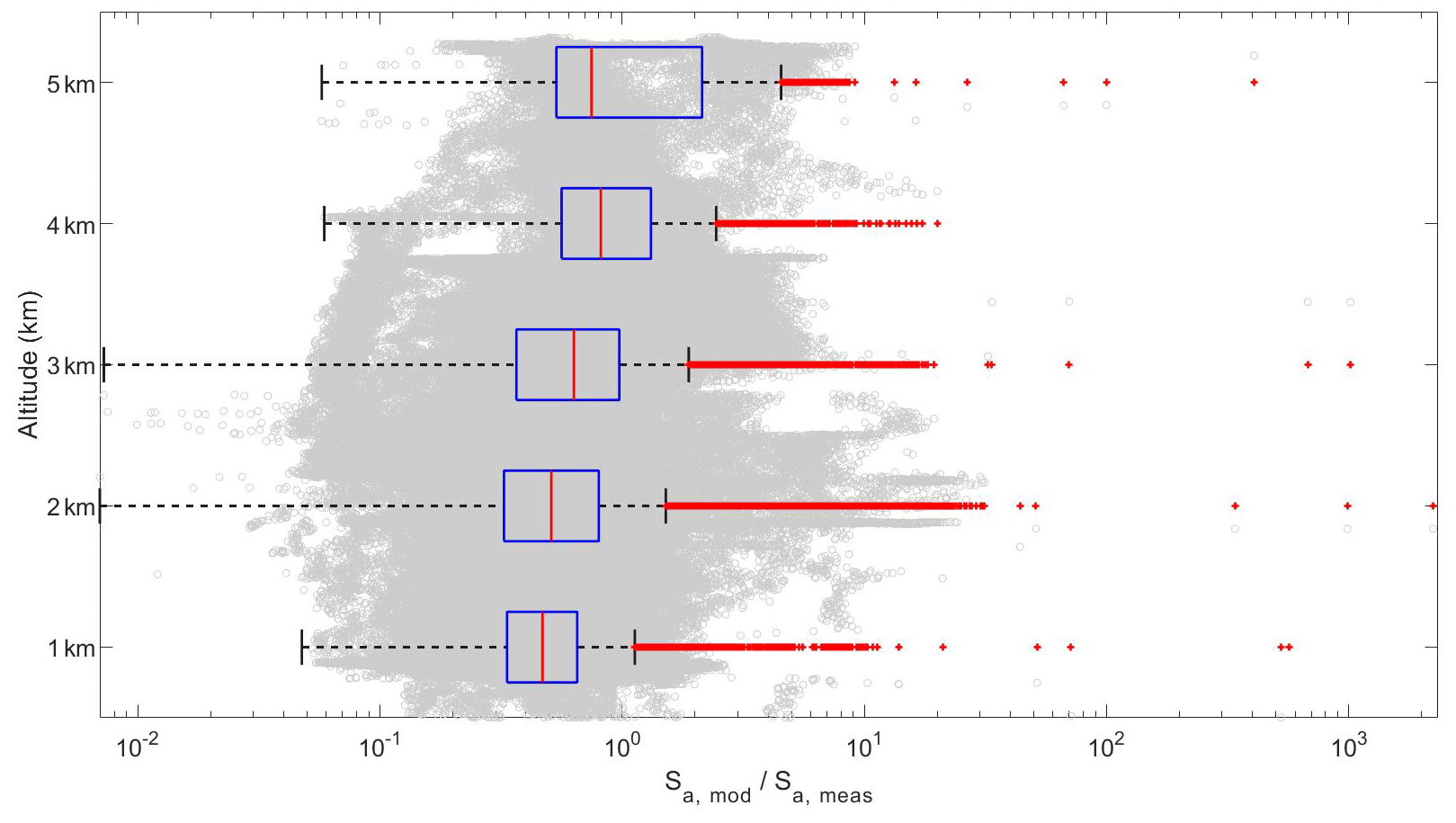
Figure 8Ratio of modeled to measured aerosol surface area concentration () including median (red line within blue box), and interquartile ranges (blue box with the 25th percentile at the left end and 75th percentile at the right end) in 1 km altitude bins. The red crosses outside of the bounds of the plot denote outliers. The labels on the altitude axis lie at the midpoint of the 1 km altitude bin.
Table 2Mean, median, and interquartile range (range of 25th to 75th percentile) surface area ratio () for each 1 km altitude bin from 0–5 km.
4.2 Dependence of on spatial and temporal resolution
The 12 km × 12 km spatial resolution and 1 h temporal resolution of CMAQ is significantly larger and longer than the spatial and temporal resolution of the aircraft data, resulting in an inherent contrast in resolution between model and measurement that may play a role in the variance in . Within any individual 12 km × 12 km model pixel, in the Baltimore–Washington sampling area, there is heterogeneity in Sa as shown in Fig. 9. Sub-grid-scale variability in Sa would lead to increased variance in but likely with a mean and median close to 1 if the domain sampling was not biased, comparable to what is observed in the CO comparison (Fig. 3), where the histogram of the CO data showcases a clear center around 1, with very few data points beyond a COmod COmeas value of 2.
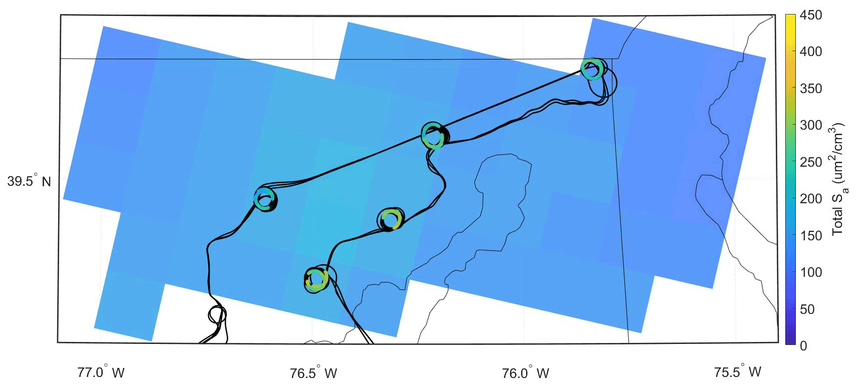
Figure 9Flight path from 28 July with overlaid UHSAS Sa data within the 10th layer of CMAQ altitude (∼ 850–1000 m) and gridded CMAQ Sa from layer 10 in the background. The CMAQ data are specifically at noon EST (16:00 UTC).
To investigate the discrepancy more quantitatively, we compare the probability density functions (PDFs) of the model-to-measured CO, NOx, particle number concentration, and particle surface area concentrations. We use the PDFs to characterize the population of data based on the standard deviation and mean, which provides a quantitative and comparable assessment of the variability in the comparison. Assuming that the research flights sampled the CMAQ model domain in an unbiased way (i.e., flights did not target or avoid point sources) we would expect that the PDFs of the modeled-to-measured ratio in CO, NOx, number concentration, and surface area concentration would all center at 1 (or log10(1) = 0 as shown in Fig. 10), and the standard deviation of the distribution (σ) would reflect heterogeneity in the scalar concentration at scales smaller than the model spatial or temporal domain. The histogram, PDF, and cumulative distribution function (CDF) for log) are shown in Fig. 10. The PDF of the histogram of log) has a mean (μ) of −0.26 and standard deviation (σ) of 0.34.

Figure 10Normalized histogram, probability density function (PDF), and cumulative distribution function (CDF) for the modeled-to-measured aerosol surface area (). The histogram and PDF serve to indicate the median and spread of the dataset, while the CDF indicates the percentage of data encompassed at a certain data threshold.
Table 3Probability density function (PDF) fit parameters for the distributions shown in Fig. 11.
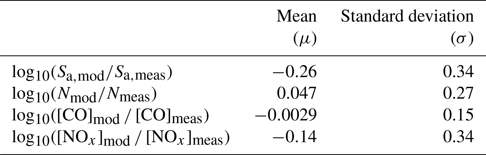
Comparison of the peak and width of the PDF of the model-to-measured ratios of CO, particle number concentration (N), and NOx provides an objective measure for assessing the impact of spatial and temporal resolution on the comparison. As shown in Fig. 11 and Table 3, the mean of each PDF is −0.0029, 0.047, and −0.14 for CO, N, and NOx. Each of these values is significantly closer to 0 than that measured for Sa (−0.26), suggesting that the methodology for assessing model–measurement agreement should not be significantly impacted by model resolution, especially given the large range in atmospheric lifetimes for CO, N, and NOx. However, without utilizing a smaller model resolution to directly test for impacts of the grid size, resolution issues cannot be fully ruled out. Interestingly, the mean is close to 1 (100.047=1.11), where a value closer to 1 indicates agreement between model and measurement and that closer to zero indicates a large discrepancy between datasets. The mean is significantly different than that observed for (10), perhaps suggesting that the model–measurement disagreement is related to the shape of the size distribution, either due to the a priori emissions size distribution or secondary aerosol processes.
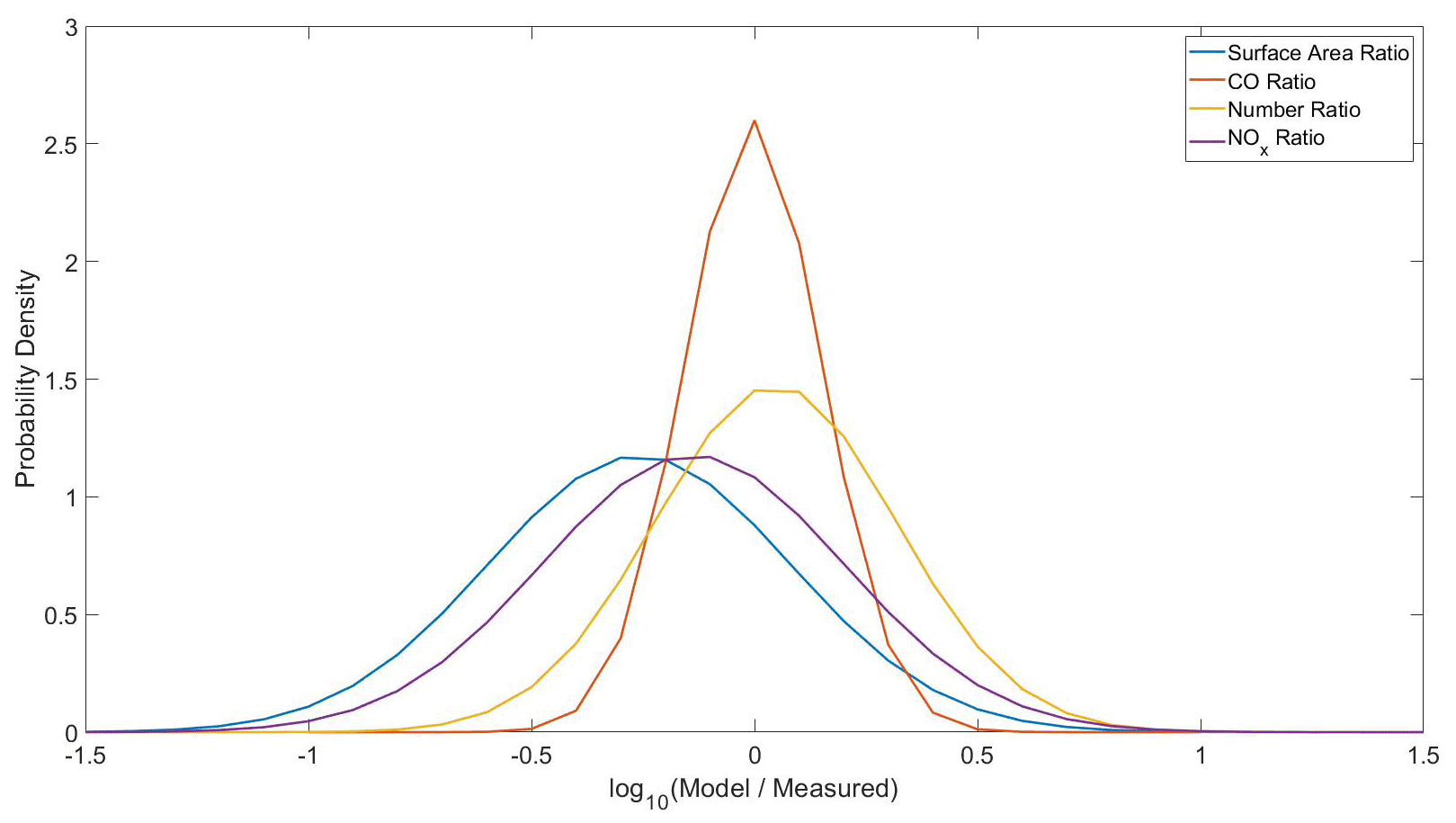
Figure 11Normalized probability density functions for the log10 of the model-to-measurement ratio in particle number concentration (yellow), carbon monoxide (red), NOx (purple), and particle surface area concentration (blue).
Also shown in Fig. 11 and Table 3, the standard deviation (σ) of the PDF for the CO, N, and NOx model-to-measurement ratios is 0.15, 0.27, and 0.34 respectively. The standard deviation of the PDF of [CO]mod [CO]meas is the narrowest, likely reflecting the longer lifetime of CO and a damping of sub-grid-scale variability of CO in each pixel. The width of the N and Sa ratio distributions is comparable, again highlighting that the deviation of from 1 may reflect differences in the modeled–measured aerosol size distribution (as shown in Fig. 1). Collectively, this analysis suggests that there is not a significant bias on average in the methodology based on model resolution and that the apparent differences in the number and surface area model–measurement ratios are most likely driven by the shape of the underlying aerosol size distribution.
It is interesting to note that the model–measurement agreement in particle number concentrations is significantly better than that of particle surface area concentrations, implying that the differences in Sa may be related to the shape of the aerosol size distribution. There have been numerous analyses of model–measurement comparison of the aerosol number concentration and size distributions specific to CMAQ (Elleman and Covert, 2009a, 2010; Kelly et al., 2011; Zhang et al., 2010b). Elleman and Covert (2009a) compared the 4 km CMAQ v4.4 model's size distributions to measurement data from the 2001 Pacific Northwest and Pacific field campaigns. The Pacific Northwest field campaign (PNW2001) was conducted in August 2001 with both airborne and ground-based measurements of pollution in the Puget Sound urban area around Seattle, Washington, and included northwest Oregon, western Washington, and southwest British Columbia. PNW2001 was conducted to complement that of the Pacific 2001 field campaign, which was a major regional air pollution study in the Lower Fraser Valley of metropolitan Vancouver, British Columbia, focusing on ground-based observations, conducted from 10 August to 2 September 2001. Analyses of these two campaigns and model predictions found that CMAQ underpredicted airborne particle number concentrations by a factor of 10–100 and was least accurate in the smallest size mode: the Aitken mode (Elleman and Covert, 2009a). The underprediction was consistent between measurement studies and did not depend on time and location. Zhang et al (2010b) compared CMAQ v4.4 to the 1999 Southern Oxidants Study and corroborated the findings of Elleman and Covert (2009a), that the Aitken mode was significantly underpredicted in total number concentration (varying by up to 3 orders of magnitude), yielding an overall underprediction of PM2.5 in Atlanta.
In a follow-up analysis, Elleman and Covert used updated emissions size distributions to compare a summer 2001 case study comprising data from a period of August 2001 with airborne and surface measurements from Pacific 2001 and PNW2001, as was used in the original base case to CMAQ (Elleman and Covert, 2010). CMAQ still underpredicted the observable aerosol number concentrations by about one order of magnitude with updated emission size distributions, which was an improvement from the 1–2 orders of magnitude previously but pointed to issues within the model's prediction of aerosol number. Kelly et al. then utilized the updated emissions size distributions from Elleman and Covert as well as the original distributions with in CMAQ to compare to the 1998 California Regional PM10 PM2.5 Air Quality Study (CRPAQS) (Kelly et al., 2011). It was noted that the simulated number size distributions from the improved emission simulation were about 20 % lower than the observations, while the standard-emission simulation was about a factor of 5 lower than the observations, confirming that the updated emissions improved model–measurement agreement. The observed shape of the distributions also better matched the updated emissions simulations. The improvement in model–measurement agreement showcases the necessity for accurate size distributions and emissions within CMAQ and the impact on Sa data.
4.3 Dependence of on secondary aerosol production
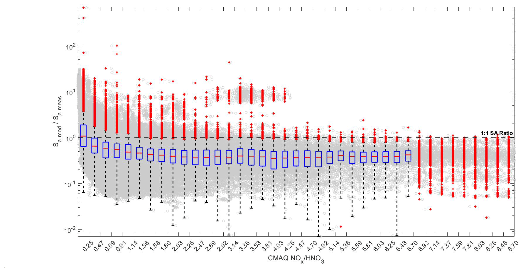
Two potential reasons for the discrepancy between mean (0.55) and mean (1.11) are (1) uncertainty in the size distribution of primary aerosol particles and (2) uncertainty in secondary aerosol production (i.e., the condensation of low-volatility material to existing aerosol particles). To investigate these two potential sources, we investigate the response of to photochemical age. We start by looking at the response of to the ratio (Fig. 12), where high in this sampling region is indicative of air masses near an anthropogenic source, similar to that of a clock (Kleinman et al., 2008; Pan et al., 2015; Tie et al., 2009). If the aerosol surface area of primary emissions is underestimated in the model, we would expect to be biased low at high . If the condensation rate of low-volatility anthropogenic species is underestimated in the model, we would expect to decrease with a decreasing ratio as the air mass ages. As shown in Fig. 12, is remarkably constant over a wide span of ratios (0.5–10), before tending to larger values at low . This trend is also seen in the dependence of on , suggesting a potential discrepancy in the modeled–measured lifetime of aerosol or treatment of background aerosol particles in the region. This trend suggests that an underestimate in the condensation of low-volatility gas-phase compounds of anthropogenic origin is not a significant driver of model–measurement discrepancy in Sa. Rather, the persistent underestimate of Sa in the model at high points to uncertainty in the size distribution of primary emissions or secondary aerosol formed at the early stages of oxidation.
To address secondary aerosol formation more generally, we also assessed the response of to temperature as equilibrium partitioning in the gas phase based on temperature and RH is a primary driver of secondary aerosol formation. No statistically significant trend in was observed over the range of temperatures observed during DISCOVER-AQ.
To further investigate secondary aerosol formation as a factor in driving the discrepancy in modeled Sa, we assess the response of to isoprene oxidation products in the aerosol phase as an example of biogenic VOC oxidation. As shown in Fig. 13, there does not appear to be a trend with concentration of isoprene SOA. Though we cannot test for all biogenic oxidation products, the lack of a trend with isoprene SOA in the aerosol phase may mean that the discrepancy in is not biogenic in nature. There is also no trend with the total SOA concentration parameterized in CMAQ, shown in Fig. 13b.

Figure 13Interquartile ranges in as a function of the modeled (CMAQ) (a) isoprene SOA concentration and (b) total SOA concentration.
As shown in E2, the rate constant for the heterogeneous loss of gas-phase compounds to aerosol (khet) is linearly dependent on both aerosol surface area concentration (Sa) and the reactive uptake coefficient (γ). In Sect. 3, we showed that the average , determined from the regression of the average model and measurement Sa was 0.437, which would result in an underestimate by approximately a factor of 2 in khet. A similar underestimation has been seen previously in select ground-based (Ghim et al., 2017; Liu and Zhang, 2011; Prank et al., 2016; Wang et al., 2021; Yu et al., 2008a, 2012, 2008b; Zhang et al., 2019, 2006, 2010c) and aircraft-based (Baker et al., 2018; Chen et al., 2020) studies of CMAQ prediction of PM2.5, which may point to a larger issue in model representation of particle mass. For some heterogeneous reactions, where the reactive uptake coefficients are well parameterized in model (e.g., extremely low-volatility species), uncertainty in Sa likely determines uncertainty in khet. To assess the dominant source of uncertainty in model-derived khet, we focus on the N2O5 system as an example. Recently, McDuffie et al. (2018) assessed the accuracy of model parameterizations of γ(N2O5) using ambient observations from the WINTER campaign. In Fig. 14a, we show the histogram and PDF of the ratio of γ(N2O5)mod calculated in CMAQ using the Bertram and Thornton (2009) parameterization for the WINTER campaign, compared with γ(N2O5)meas, which was determined in McDuffie et al. (2018) from an observationally constrained analysis of flight data via a box model solved along the flight path to determine the uptake coefficient. The PDF of the directly compared model–measurement ratio is centered above zero (μ=0.22 or γ(N2O(N2O5)meas=1.65) (Fig. 14, Table 3). Interestingly, since khet(N2O5) is proportional to the product of Sa and γ(N2O5), the underestimate in model Sa is compensated for by an overestimate in γ (N2O5) in the mean state if the underestimate in model Sa is consistent for WINTER, though that is not necessarily the case. While the width of the PDF of log10(γ(N2O5)(N2O5)meas) for WINTER is similar to that seen for Sa for DISCOVER-AQ, it should be noted that neither the histogram of the γ(N2O5) ratio or the Sa ratio is easily fit to a Gaussian peak shape. As shown in Fig. 14, the histogram of the log10(γ(N2O(N2O5)meas) for WINTER has a broader range of values than that of Sa in this study. Collectively, this analysis highlights that while model uncertainty in khet(N2O5) is largely a function of quality of the γ(N2O5) parameterization, future improvements in modeled surface area concentrations, particularly in urban environments, will also result in more accurate representations of heterogeneous chemical reactions.
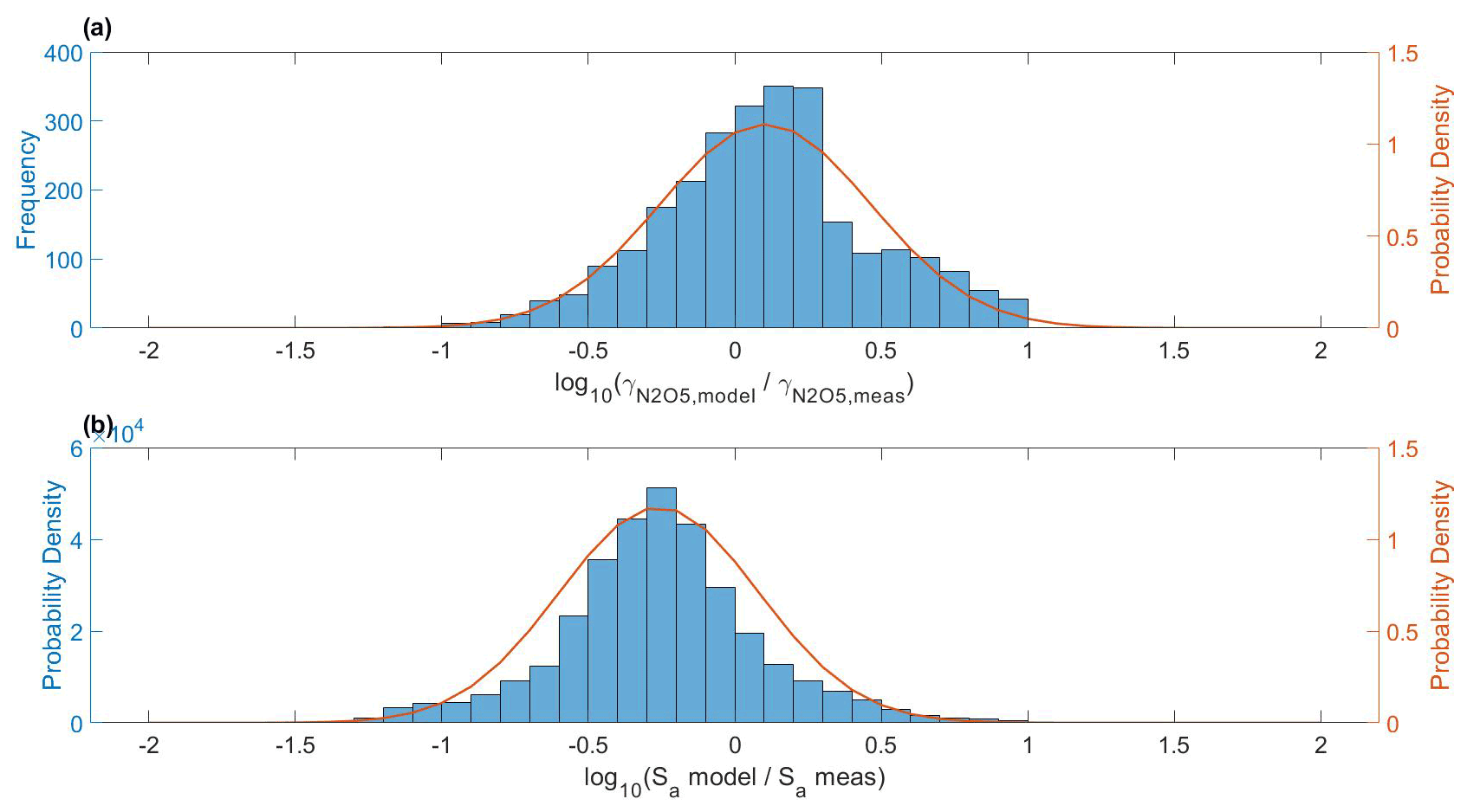
Figure 14Normalized probability density functions for the log10 of the model-to-measurement ratio in (a) γ(N2O5) from the WINTER campaign and (b) particle surface area concentration, Sa, from this study.
This study examined the ability of the CMAQ model to accurately predict aerosol surface area as it directly affects heterogeneous chemistry within the model. The CMAQ data were compared to dry measured aerosol surface area data from the 2011 DISCOVER-AQ campaign utilizing a UHSAS. Showing a discrepancy between modeled and measured dry aerosol surface area, Sa,mod and Sa,meas, respectively, are modestly correlated (r2=0.52) and on average agree to within a factor of 2 () over the course of the 13 research flights. However, there was a strong correlation between measured and modeled number concentration (, r2=0.63). When looking into possible sources of the discrepancy, there was not a strong dependence on photochemical age or secondary biogenic aerosol concentration. The strong agreement in aerosol number concentration may indicate that the modeled size distribution contributes to the observed discrepancy, though the exact source of discrepancy is outside of the scope of this study.
The discrepancy in aerosol surface area was also compared to that of the reactive uptake coefficient of N2O5 during the 2015 WINTER campaign due to the fact that the uptake coefficient also directly impacts heterogeneous reaction rates. The uncertainty in the modeled heterogeneous chemistry remains primarily driven by that of the uptake coefficient, as the uncertainty in those values is larger than that seen by Sa. Model improvements to aerosol surface area concentrations along with improvements to the parameterization of reactive uptake coefficients will greatly impact the accuracy of heterogeneous chemistry within regional models.
Data from the 2011 DISCOVER-AQ campaign are publicly available at https://doi.org/10.5067/Aircraft/DISCOVER-AQ/Aerosol-TraceGas (NASA/LARC/SD/ASDC, 2014). CMAQ output data are available on the University of Wisconsin – Madison MINDS database at https://minds.wisconsin.edu/handle/1793/83241 (Bertram and Bergin, 2022).
The supplement related to this article is available online at: https://doi.org/10.5194/acp-22-15449-2022-supplement.
MH, AH, and TH ran the CMAQ model and assisted with analysis of model outputs. RAB analyzed the model and measurement data. RAB and THB wrote the paper. All authors reviewed and edited the paper.
At least one of the (co-)authors is a member of the editorial board of Atmospheric Chemistry and Physics. The peer-review process was guided by an independent editor, and the authors also have no other competing interests to declare.
The paper has not been formally reviewed by EPA. The views expressed in this document are solely those of the authors of this publication and do not necessarily reflect those of the Agency. EPA does not endorse any products or commercial services mentioned in this publication.
Publisher's note: Copernicus Publications remains neutral with regard to jurisdictional claims in published maps and institutional affiliations.
We would like to thank Heather Simon and Lyatt Jaeglé for their data contributions and Erin McDuffie and Steve Brown for the use of the WINTER data in this work.
This publication was developed under Assistance Agreement No. R840006 awarded by the U.S. Environmental Protection Agency to The University of Wisconsin-Madison. This research was also supported by the NOAA Climate Program Office's Atmospheric Chemistry, Carbon Cycle, and Climate program (NA18OAR4310109). The NASA LARGE research team was supported by funding from the NASA Earth Venture Suborbital-1 Program.
This paper was edited by Qi Chen and reviewed by two anonymous referees.
Abbatt, J. P. D., Lee, A. K. Y., and Thornton, J. A.: Quantifying trace gas uptake to tropospheric aerosol: recent advances and remaining challenges, Chem. Soc. Rev., 41, 6555–6581, https://doi.org/10.1039/c2cs35052a, 2012.
Abel, D. W., Holloway, T., Harkey, M., Meier, P., Ahl, D., Limaye, V. S., and Patz, J. A.: Air-quality-related health impacts from climate change and from adaptation of cooling demand for buildings in the eastern United States: An interdisciplinary modeling study, PLoS Med., 15, 1–27, https://doi.org/10.1371/journal.pmed.1002599, 2018.
Abel, D. W., Holloway, T., Martínez-Santos, J., Harkey, M., Tao, M., Kubes, C., and Hayes, S.: Air Quality-Related Health Benefits of Energy Efficiency in the United States, Environ. Sci. Technol., 53, 3987–3998, https://doi.org/10.1021/acs.est.8b06417, 2019.
Adams, P. J. and Seinfeld, J. H.: Predicting global aerosol size distributions in general circulation models, J. Geophys. Res.-Atmos., 107(19), AAC 4-1-AAC 4-23, https://doi.org/10.1029/2001JD001010, 2002.
Appel, K. W., Bash, J. O., Fahey, K. M., Foley, K. M., Gilliam, R. C., Hogrefe, C., Hutzell, W. T., Kang, D., Mathur, R., Murphy, B. N., Napelenok, S. L., Nolte, C. G., Pleim, J. E., Pouliot, G. A., Pye, H. O. T., Ran, L., Roselle, S. J., Sarwar, G., Schwede, D. B., Sidi, F. I., Spero, T. L., and Wong, D. C.: The Community Multiscale Air Quality (CMAQ) model versions 5.3 and 5.3.1: system updates and evaluation, Geosci. Model Dev., 14, 2867–2897, https://doi.org/10.5194/gmd-14-2867-2021, 2021.
Baker, K. R., Woody, M. C., Valin, L., Szykman, J., Yates, E. L., Iraci, L. T., Choi, H. D., Soja, A. J., Koplitz, S. N., Zhou, L., Campuzano-Jost, P., Jimenez, J. L., and Hair, J. W.: Photochemical model evaluation of 2013 California wild fire air quality impacts using surface, aircraft, and satellite data, Sci. Total Environ., 637–638, 1137–1149, https://doi.org/10.1016/j.scitotenv.2018.05.048, 2018.
Bates, T. S., Quinn, P. K., Coffman, D., Schulz, K., Covert, D. S., Johnson, J. E., Williams, E. J., Lerner, B. M., Angevine, W. M., Tucker, S. C., Brewer, W. A., and Stohl, A.: Boundary layer aerosol chemistry during TexAQS/GoMACCS 2006: Insights into aerosol sources and transformation processes, J. Geophys. Res., 113, 1–18, https://doi.org/10.1029/2008jd010023, 2008.
Bertram, T. H. and Bergin, R. A.: Observation-based constraints on modeled aerosol surface area, MINDS@UW [data set], https://minds.wisconsin.edu/handle/1793/83241, last access: 27 May 2022.
Bertram, T. H. and Thornton, J. A.: Toward a general parameterization of N2O5 reactivity on aqueous particles: the competing effects of particle liquid water, nitrate and chloride, Atmos. Chem. Phys., 9, 8351–8363, https://doi.org/10.5194/acp-9-8351-2009, 2009.
Binkowski, F. S.: Chapter 10 – AEROSOLS IN MODELS-3 CMAQ, in: SCIENCE ALGORITHMS OF THE EPA MODELS-3 COMMUNITY MULTISCALE AIR QUALITY (CMAQ) MODELING SYSTEM, edited by: Byun, D. W. and Ching, J. K. S., 10-1–10-23, U.S. Environmental Protection Agency, Washington, DC., EPA/600/R-99/030 (NTIS PB2000-100561), 1999.
Binkowski, F. S. and Roselle, S. J.: Models-3 Community Multiscale Air Quality (CMAQ) model aerosol component, 1, Model description, J. Geophys. Res., 108, 4183, https://doi.org/10.1029/2001JD001409, 2003.
Brown, S. S., Dubé, W. P., Fuchs, H., Ryerson, T. B., Wollny, A. G., Brock, C. A., Bahreini, R., Middlebrook, A. M., Neuman, T. A., Atlas, E., Roberts, J. M., Osthoff, H. D., Trainer, M., Fehsenfeld, F. C., and Ravishankara, A. R.: Reactive uptake coefficients for N2O5 determined from aircraft measurements during the Second Texas Air Quality Study: Comparison to current model parameterizations, J. Geophys. Res.-Atmos., 114, 1–16, https://doi.org/10.1029/2008JD011679, 2009.
Byun, D. and Schere, K. L.: Review of the governing equations, computational algorithms, and other components of the Models-3 Community Multiscale Air Quality (CMAQ) modeling, Appl. Mech. Rev., 59, 51–77, https://doi.org/10.1115/1.2128636, 2006.
Carlton, A. G., Bhave, P. V., Napelenok, S. L., Edney, E. O., Sarwar, G., Pinder, R. W., Pouliot, G. A., and Houyoux, M.: Model representation of secondary organic aerosol in CMAQv4.7, Environ. Sci. Technol., 44, 8553–8560, https://doi.org/10.1021/es100636q, 2010.
Chang, W. L., Bhave, P. V., Brown, S. S., Riemer, N., Stutz, J., and Dabdub, D.: Heterogeneous atmospheric chemistry, ambient measurements, and model calculations of N2O5: A review, Aerosol Sci. Technol., 45, 665–695, https://doi.org/10.1080/02786826.2010.551672, 2011.
Chen, J., Yin, D., Zhao, Z., Kaduwela, A. P., Avise, J. C., DaMassa, J. A., Beyersdorf, A., Burton, S., Ferrare, R., Herman, J. R., Kim, H., Neuman, A., Nowak, J. B., Parworth, C., Scarino, A. J., Wisthaler, A., Young, D. E., and Zhang, Q.: Modeling air quality in the San Joaquin valley of California during the 2013 Discover-AQ field campaign, Atmos. Environ. X, 5, 100067, https://doi.org/10.1016/j.aeaoa.2020.100067, 2020.
Crawford, J. H. and Pickering, K. E.: DISCOVER-AQ: Advancing strategies for air quality observations in the next decade, EM Air Waste Manag. Assoc. Mag. Environ. Manag., 4–7, https://pubs.awma.org/flip/EM-Sept-2014/emsept14.pdf (last access: 29 November 2022), 2014.
Crawford, J. H., Dickerson, R. R., and Hains, J. C.: DISCOVER-AQ: Observations and early results, EM Air Waste Manag. Assoc. Mag. Environ. Manag., 8–15, https://pubs.awma.org/flip/EM-Sept-2014/emsept14.pdf (last access: 29 November 2022), 2014.
Davis, J. M., Bhave, P. V., and Foley, K. M.: Parameterization of N2O5 reaction probabilities on the surface of particles containing ammonium, sulfate, and nitrate, Atmos. Chem. Phys., 8, 5295–5311, https://doi.org/10.5194/acp-8-5295-2008, 2008.
Donahue, N. M., Robinson, A. L., Trump, E. R., Riipinen, I., and Kroll, J. H.: Volatility and Aging of Atmospheric Organic Aerosol, in: Atmospheric and Aerosol Chemistry, edited by: McNeill, V. F. and Ariya, P. A., 97–143, Springer Berlin Heidelberg, Berlin, Heidelberg, https://doi.org/10.1007/128_2012_355, 2012.
Elleman, R. A. and Covert, D. S.: Aerosol size distribution modeling with the Community Multiscale Air Quality modeling system in the Pacific Northwest: 1. Model comparison to observations, J. Geophys. Res.-Atmos., 114, D11206, https://doi.org/10.1029/2008JD010791, 2009a.
Elleman, R. A. and Covert, D. S.: Aerosol size distribution modeling with the Community Multiscale Air Quality modeling system in the Pacific Northwest: 2. Parameterizations for ternary nucleation and nucleation mode processes, J. Geophys. Res., 114, D11207, https://doi.org/10.1029/2009JD012187, 2009b.
Elleman, R. A. and Covert, D. S.: Aerosol size distribution modeling with the Community Multiscale Air Quality modeling system in the Pacific Northwest: 3. Size distribution of particles emitted into a mesoscale model, J. Geophys. Res.-Atmos., 115, 1–14, https://doi.org/10.1029/2009JD012401, 2010.
Emery, C., Jung, J., Koo, B., and Yarwood, G.: Improvements to CAMx snow cover treatments and carbon bond chemical mechanism for winter ozone, Ramboll Environ, 43 pp., Report Number UDAQ PO 480 52000000001, https://www.camx.com/files/udaq_snowchem_final_6aug15.pdf (last access: 29 November 2022), 2015.
Emmons, L. K., Walters, S., Hess, P. G., Lamarque, J.-F., Pfister, G. G., Fillmore, D., Granier, C., Guenther, A., Kinnison, D., Laepple, T., Orlando, J., Tie, X., Tyndall, G., Wiedinmyer, C., Baughcum, S. L., and Kloster, S.: Description and evaluation of the Model for Ozone and Related chemical Tracers, version 4 (MOZART-4), Geosci. Model Dev., 3, 43–67, https://doi.org/10.5194/gmd-3-43-2010, 2010.
Evans, M. J. and Jacob, D. J.: Impact of new laboratory studies of N2O5 hydrolysis on global model budgets of tropospheric nitrogen oxides, ozone, and OH, Geophys. Res. Lett., 32, 1–4, https://doi.org/10.1029/2005GL022469, 2005.
Fan, J., Zhang, R., Li, G., Nielsen-Gammon, J., and Li, Z.: Simulations of fine particulate matter (PM2.5) in Houston, Texas, J. Geophys. Res. D Atmos., 110, 1–9, https://doi.org/10.1029/2005JD005805, 2005.
Foley, K. M., Roselle, S. J., Appel, K. W., Bhave, P. V., Pleim, J. E., Otte, T. L., Mathur, R., Sarwar, G., Young, J. O., Gilliam, R. C., Nolte, C. G., Kelly, J. T., Gilliland, A. B., and Bash, J. O.: Incremental testing of the Community Multiscale Air Quality (CMAQ) modeling system version 4.7, Geosci. Model Dev., 3, 205–226, https://doi.org/10.5194/gmd-3-205-2010, 2010.
Gantt, B., Johnson, M. S., Meskhidze, N., Sciare, J., Ovadnevaite, J., Ceburnis, D., and O'Dowd, C. D.: Model evaluation of marine primary organic aerosol emission schemes, Atmos. Chem. Phys., 12, 8553–8566, https://doi.org/10.5194/acp-12-8553-2012, 2012.
Gaston, C. J., Riedel, T. P., Zhang, Z., Gold, A., Surratt, J. D., and Thornton, J. A.: Reactive uptake of an isoprene-derived epoxydiol to submicron aerosol particles, Environ. Sci. Technol., 48, 11178–11186, https://doi.org/10.1021/es5034266, 2014.
Gelbard, F., Tambour, Y., and Seinfeld, J. H.: Sectional representations for simulating aerosol dynamics, J. Colloid Interface Sci., 76, 541–556, https://doi.org/10.1016/0021-9797(80)90394-X, 1980.
George, I. J., Matthews, P. S. J., Whalley, L. K., Brooks, B., Goddard, A., Baeza-Romero, M. T., and Heard, D. E.: Measurements of uptake coefficients for heterogeneous loss of HO2 onto submicron inorganic salt aerosols, Phys. Chem. Chem. Phys., 15, 12829–12845, https://doi.org/10.1039/c3cp51831k, 2013.
Geyer, A. and Stutz, J.: Vertical profiles of NO3, N2O5, O3, and NOx in the nocturnal boundary layer: 2. Model studies on the altitude dependence of composition and chemistry, J. Geophys. Res. D Atmos., 109, 1–18, https://doi.org/10.1029/2003JD004211, 2004.
Ghan, S., Laulainen, N., Easter, R., Wagener, R., Nemesure, S., Chapman, E., Zhang, Y., and Leung, R.: Evaluation of aerosol direct radiative forcing in MIRAGE, J. Geophys. Res., 106, 5295–5316, 2001.
Ghim, Y. S., Choi, Y., Kim, S., Bae, C. H., Park, J., and Shin, H. J.: Evaluation of model performance for forecasting fine particle concentrations in Korea, Aerosol Air Qual. Res., 17, 1856–1864, https://doi.org/10.4209/aaqr.2016.10.0446, 2017.
Guenther, A. B., Jiang, X., Heald, C. L., Sakulyanontvittaya, T., Duhl, T., Emmons, L. K., and Wang, X.: The Model of Emissions of Gases and Aerosols from Nature version 2.1 (MEGAN2.1): an extended and updated framework for modeling biogenic emissions, Geosci. Model Dev., 5, 1471–1492, https://doi.org/10.5194/gmd-5-1471-2012, 2012.
Harkey, M., Holloway, T., Kim, E. J., Baker, K. R., and Henderson, B.: Satellite Formaldehyde to Support Model Evaluation, J. Geophys. Res.-Atmos., 126, 1–18, https://doi.org/10.1029/2020JD032881, 2021.
Hogrefe, C., Lynn, B., Goldberg, R., Rosenzweig, C., Zalewsky, E., Hao, W., Doraiswamy, P., Civerolo, K., Ku, J. Y., Sistla, G., and Kinney, P. L.: A combined model-observation approach to estimate historic gridded fields of PM2.5 mass and species concentrations, Atmos. Environ., 43, 2561–2570, https://doi.org/10.1016/j.atmosenv.2009.02.031, 2009.
Hogrefe, C., Pouliot, G., Wong, D., Torian, A., Roselle, S., Pleim, J., and Mathur, R.: Annual application and evaluation of the online coupled WRF-CMAQ system over North America under AQMEII phase 2, Atmos. Environ., 115, 683–694, https://doi.org/10.1016/j.atmosenv.2014.12.034, 2015.
Jacobson, M. Z.: GATOR-GCMM: A global- through urban-scale air pollution and weather forecast model 1. Model design and treatment of subgrid soil, vegetation, roads, rooftops, water, sea ice, and snow, J. Geophys. Res.-Atmos., 106, 5385–5401, https://doi.org/10.1029/2000JD900560, 2001.
Jaeglé, L., Shah, V., Thornton, J. A., Lopez-Hilfiker, F. D., Lee, B. H., McDuffie, E. E., Fibiger, D., Brown, S. S., Veres, P., Sparks, T. L., Ebben, C. J., Wooldridge, P. J., Kenagy, H. S., Cohen, R. C., Weinheimer, A. J., Campos, T. L., Montzka, D. D., Digangi, J. P., Wolfe, G. M., Hanisco, T., Schroder, J. C., Campuzano-Jost, P., Day, D. A., Jimenez, J. L., Sullivan, A. P., Guo, H., and Weber, R. J.: Nitrogen Oxides Emissions, Chemistry, Deposition, and Export Over the Northeast United States During the WINTER Aircraft Campaign, J. Geophys. Res.-Atmos., 123, 12368–12393, https://doi.org/10.1029/2018JD029133, 2018.
Kelly, J. T., Avise, J., Cai, C., and Kaduwela, A. P.: Simulating particle size distributions over California and impact on lung deposition fraction, Aerosol Sci. Technol., 45, 148–162, https://doi.org/10.1080/02786826.2010.528078, 2011.
Kleeman, M. J., Cass, G. R., and Eldering, A.: Modeling the airborne particle complex as a source-oriented external mixture, J. Geophys. Res.-Atmos., 102, 21355–21372, https://doi.org/10.1029/97jd01261, 1997.
Kleinman, L. I., Springston, S. R., Daum, P. H., Lee, Y.-N., Nunnermacker, L. J., Senum, G. I., Wang, J., Weinstein-Lloyd, J., Alexander, M. L., Hubbe, J., Ortega, J., Canagaratna, M. R., and Jayne, J.: The time evolution of aerosol composition over the Mexico City plateau, Atmos. Chem. Phys., 8, 1559–1575, https://doi.org/10.5194/acp-8-1559-2008, 2008.
Knote, C., Brunner, D., Vogel, H., Allan, J., Asmi, A., Äijälä, M., Carbone, S., van der Gon, H. D., Jimenez, J. L., Kiendler-Scharr, A., Mohr, C., Poulain, L., Prévôt, A. S. H., Swietlicki, E., and Vogel, B.: Towards an online-coupled chemistry-climate model: evaluation of trace gases and aerosols in COSMO-ART, Geosci. Model Dev., 4, 1077–1102, https://doi.org/10.5194/gmd-4-1077-2011, 2011.
Kulmala, M., Laaksonen, A., and Pirjola, L.: Parameterizations for sulfuric acid/water nucleation rates, J. Geophys. Res.-Atmos., 103, 8301–8307, https://doi.org/10.1029/97JD03718, 1998.
Lakey, P. S. J., George, I. J., Whalley, L. K., Baeza-Romero, M. T., and Heard, D. E.: Measurements of the HO2 Uptake Coefficients onto Single Component Organic Aerosols, Environ. Sci. Technol., 49, 4878–4885, https://doi.org/10.1021/acs.est.5b00948, 2015.
Lee, Y. H. and Adams, P. J.: A fast and efficient version of the TwO-Moment Aerosol Sectional (TOMAS) global aerosol microphysics model, Aerosol Sci. Technol., 46, 678–689, https://doi.org/10.1080/02786826.2011.643259, 2012.
Lee, Y. H., Chen, K., and Adams, P. J.: Development of a global model of mineral dust aerosol microphysics, Atmos. Chem. Phys., 9, 2441–2458, https://doi.org/10.5194/acp-9-2441-2009, 2009.
Liu, P. and Zhang, Y.: Use of a process analysis tool for diagnostic study on fine particulate matter predictions in the U.S. – Part I: Model evaluation, Atmos. Pollut. Res., 2, 49–60, https://doi.org/10.5094/APR.2011.007, 2011.
Luecken, D. J., Yarwood, G., and Hutzell, W. T.: Multipollutant modeling of ozone, reactive nitrogen and HAPs across the continental US with CMAQ-CB6, Atmos. Environ., 201, 62–72, https://doi.org/10.1016/j.atmosenv.2018.11.060, 2019.
Luo, G. and Yu, F.: Simulation of particle formation and number concentration over the Eastern United States with the WRF-Chem + APM model, Atmos. Chem. Phys., 11, 11521–11533, https://doi.org/10.5194/acp-11-11521-2011, 2011.
Macintyre, H. L. and Evans, M. J.: Sensitivity of a global model to the uptake of N2O5 by tropospheric aerosol, Atmos. Chem. Phys., 10, 7409–7414, https://doi.org/10.5194/acp-10-7409-2010, 2010.
Mann, G. W., Carslaw, K. S., Spracklen, D. V., Ridley, D. A., Manktelow, P. T., Chipperfield, M. P., Pickering, S. J., and Johnson, C. E.: Description and evaluation of GLOMAP-mode: a modal global aerosol microphysics model for the UKCA composition-climate model, Geosci. Model Dev., 3, 519–551, https://doi.org/10.5194/gmd-3-519-2010, 2010.
Martin, R. V, Jacob, D. J., Yantosca, R. M., Chin, M., and Ginoux, P.: Global and regional decreases in tropospheric oxidants from photochemical effects of aerosols, J. Geophys. Res., 108, 4097, https://doi.org/10.1029/2002JD002622, 2003.
McDuffie, E. E., Fibiger, D. L., Dubé, W. P., Lopez-Hilfiker, F., Lee, B. H., Thornton, J. A., Shah, V., Jaeglé, L., Guo, H., Weber, R. J., Michael Reeves, J., Weinheimer, A. J., Schroder, J. C., Campuzano-Jost, P., Jimenez, J. L., Dibb, J. E., Veres, P., Ebben, C., Sparks, T. L., Wooldridge, P. J., Cohen, R. C., Hornbrook, R. S., Apel, E. C., Campos, T., Hall, S. R., Ullmann, K., and Brown, S. S.: Heterogeneous N2O5 Uptake During Winter: Aircraft Measurements During the 2015 WINTER Campaign and Critical Evaluation of Current Parameterizations, J. Geophys. Res.-Atmos., 123, 4345–4372, https://doi.org/10.1002/2018JD028336, 2018.
Meng, Z.: of Atmospheric Aerosol Dynamics, Environ. Eng., 103, 3419–3435, 1998.
Messinger, F., DiMego, G., Kalnay, E., Mitchell, K., Shafran, P. C., Ebisuzaki, W., Jović, D., Woollen, J., Rogers, E., Berbery, E. H., Ek, M. B., Fan, Y., Grumbine, R., Higgins, W., Li, H., Lin, Y., Manikin, G., Parrish, D., and Shi, W.: North American Regional Reanalysis, B. Am. Meteorol. Soc., 87, 343–360, https://doi.org/10.1175/BAMS-87-3-343, 2006.
Moore, R. H., Wiggins, E. B., Ahern, A. T., Zimmerman, S., Montgomery, L., Campuzano Jost, P., Robinson, C. E., Ziemba, L. D., Winstead, E. L., Anderson, B. E., Brock, C. A., Brown, M. D., Chen, G., Crosbie, E. C., Guo, H., Jimenez, J. L., Jordan, C. E., Lyu, M., Nault, B. A., Rothfuss, N. E., Sanchez, K. J., Schueneman, M., Shingler, T. J., Shook, M. A., Thornhill, K. L., Wagner, N. L., and Wang, J.: Sizing response of the Ultra-High Sensitivity Aerosol Spectrometer (UHSAS) and Laser Aerosol Spectrometer (LAS) to changes in submicron aerosol composition and refractive index, Atmos. Meas. Tech., 14, 4517–4542, https://doi.org/10.5194/amt-14-4517-2021, 2021.
NASA: DISCOVER-AQ: Diagnosing the Air We Breathe, http://www.nasa.gov/discover-aq (last access: 11 April 2022), 2012.
NASA/LARC/SD/ASDC: DISCOVER-AQ P-3B Aircraft in-situ Trace Gas Measurements, NASA Langley Atmospheric Science Data Center DAAC [data set], https://doi.org/10.5067/AIRCRAFT/DISCOVER-AQ/AEROSOL-TRACEGAS, 2014.
NEIC: National Emissions Inventory Collaborative, 2016v1 Emiss. Model. Platf, http://views.cira.colostate.edu/wiki/wiki/10202 (last access: 3 November 2021), 2019.
Nolte, C. G., Appel, K. W., Kelly, J. T., Bhave, P. V., Fahey, K. M., Collett Jr., J. L., Zhang, L., and Young, J. O.: Evaluation of the Community Multiscale Air Quality (CMAQ) model v5.0 against size-resolved measurements of inorganic particle composition across sites in North America, Geosci. Model Dev., 8, 2877–2892, https://doi.org/10.5194/gmd-8-2877-2015, 2015.
Pan, X., Kanaya, Y., Tanimoto, H., Inomata, S., Wang, Z., Kudo, S., and Uno, I.: Examining the major contributors of ozone pollution in a rural area of the Yangtze River Delta region during harvest season, Atmos. Chem. Phys., 15, 6101–6111, https://doi.org/10.5194/acp-15-6101-2015, 2015.
Park, S. K., Marmur, A., Kim, S. B., Tian, D., Hu, Y., McMurry, P. H., and Russell, A. G.: Evaluation of fine particle number concentrations in CMAQ, Aerosol Sci. Technol., 40, 985–996, https://doi.org/10.1080/02786820600907353, 2006.
Portmann, R. W., Solomon, S., Garcia, R. R., Thomason, L. W., Poole, L. R., and McCormick, M. P.: Role of aerosol variations in anthropogenic ozone depletion in the polar regions, J. Geophys. Res.-Atmos., 101, 22991–23006, https://doi.org/10.1029/96jd02608, 1996.
Prank, M., Sofiev, M., Tsyro, S., Hendriks, C., Semeena, V., Vazhappilly Francis, X., Butler, T., Denier van der Gon, H., Friedrich, R., Hendricks, J., Kong, X., Lawrence, M., Righi, M., Samaras, Z., Sausen, R., Kukkonen, J., and Sokhi, R.: Evaluation of the performance of four chemical transport models in predicting the aerosol chemical composition in Europe in 2005, Atmos. Chem. Phys., 16, 6041–6070, https://doi.org/10.5194/acp-16-6041-2016, 2016.
Pringle, K. J., Tost, H., Message, S., Steil, B., Giannadaki, D., Nenes, A., Fountoukis, C., Stier, P., Vignati, E., and Lelieveld, J.: Description and evaluation of GMXe: a new aerosol submodel for global simulations (v1), Geosci. Model Dev., 3, 391–412, https://doi.org/10.5194/gmd-3-391-2010, 2010.
Pye, H. O. T., Luecken, D. J., Xu, L., Boyd, C. M., Ng, N. L., Baker, K. R., Ayres, B. R., Bash, J. O., Baumann, K., Carter, W. P. L., Edgerton, E., Fry, J. L., Hutzell, W. T., Schwede, D. B., and Shepson, P. B.: Modeling the current and future roles of particulate organic nitrates in the southeastern United States, Environ. Sci. Technol., 49, 14195–14203, https://doi.org/10.1021/acs.est.5b03738, 2015.
Pye, H. O. T., Murphy, B. N., Xu, L., Ng, N. L., Carlton, A. G., Guo, H., Weber, R., Vasilakos, P., Appel, K. W., Budisulistiorini, S. H., Surratt, J. D., Nenes, A., Hu, W., Jimenez, J. L., Isaacman-VanWertz, G., Misztal, P. K., and Goldstein, A. H.: On the implications of aerosol liquid water and phase separation for organic aerosol mass, Atmos. Chem. Phys., 17, 343–369, https://doi.org/10.5194/acp-17-343-2017, 2017.
Qin, M., Murphy, B. N., Isaacs, K. K., McDonald, B. C., Lu, Q., McKeen, S. A., Koval, L., Robinson, A. L., Efstathiou, C., Allen, C., and Pye, H. O. T.: Criteria pollutant impacts of volatile chemical products informed by near-field modeling, Nat. Sustain., 4, 129–137, https://doi.org/10.1038/s41893-020-00614-1, 2021.
Ranjithkumar, A., Gordon, H., Williamson, C., Rollins, A., Pringle, K., Kupc, A., Abraham, N. L., Brock, C., and Carslaw, K.: Constraints on global aerosol number concentration, SO2 and condensation sink in UKESM1 using ATom measurements, Atmos. Chem. Phys., 21, 4979–5014, https://doi.org/10.5194/acp-21-4979-2021, 2021.
Ridley, B. A. and Grahek, F. E.: A small, low-flow, high-sensitivity reaction vessel for NO chemiluminescence detectors, J. Atmos. Ocean. Technol., 7, 307–311, https://doi.org/10.1175/1520-0426(1990)007<0307:aslfhs>2.0.co;2, 1990.
Sachse, G., Hill, G., Wade, L., and Perry, M.: Fast-response, high-precision carbon monoxide sensor using a tunable diode laser absorption technique, J. Geophys. Res.-Atmos., 92, 2071–2081, https://doi.org/10.1029/JD092iD02p02071, 1987.
Sartelet, K. N., Hayami, H., Albriet, B., and Sportisse, B.: Development and preliminary validation of a modal aerosol model for tropospheric chemistry: MAM, Aerosol Sci. Technol., 40, 118–127, https://doi.org/10.1080/02786820500485948, 2006.
Simon, H., Kimura, Y., McGaughey, G., Allen, D. T., Brown, S. S., Coffman, D., Dibb, J., Osthoff, H. D., Quinn, P., Roberts, J. M., Yarwood, G., Kemball-Cook, S., Byun, D., and Lee, D.: Modeling heterogeneous ClNO2 formation, chloride availability, and chlorine cycling in Southeast Texas, Atmos. Environ., 44, 5476–5488, https://doi.org/10.1016/j.atmosenv.2009.09.006, 2010.
Skamarock, W. C., Klemp, J. B., Dudhia, J., Gill, D. O., Barker, D. M., Duda, M. G., Huang, X.-Y., Wang, W., and Powers, J. G.: A description of the Advanced Research WRF Version 3, 113 pp., NCAR Tech. Note NCAR/TN-475+STR, https://doi.org/10.5065/D68S4MVH, 2008.
Smyth, S. C., Jiang, W., Yin, D., Roth, H., and Giroux, É.: Evaluation of CMAQ O3 and PM2.5 performance using Pacific 2001 measurement data, Atmos. Environ., 40, 2735–2749, https://doi.org/10.1016/j.atmosenv.2005.10.068, 2006.
Sonntag, D. B., Baldauf, R. W., Yanca, C. A., and Fulper, C. R.: Particulate matter speciation profiles for light-duty gasoline vehicles in the United States, J. Air Waste Manage. Assoc., 64, 529–545, https://doi.org/10.1080/10962247.2013.870096, 2014.
Spak, S. N. and Holloway, T.: Seasonality of speciated aerosol transport over the Great Lakes region, J. Geophys. Res.-Atmos., 114, 1–18, https://doi.org/10.1029/2008JD010598, 2009.
Spracklen, D. V., Carslaw, K. S., Kulmala, M., Kerminen, V.-M., Mann, G. W., and Sihto, S.-L.: The contribution of boundary layer nucleation events to total particle concentrations on regional and global scales, Atmos. Chem. Phys., 6, 5631–5648, https://doi.org/10.5194/acp-6-5631-2006, 2006.
Stadtler, S., Simpson, D., Schröder, S., Taraborrelli, D., Bott, A., and Schultz, M.: Ozone impacts of gas–aerosol uptake in global chemistry transport models, Atmos. Chem. Phys., 18, 3147–3171, https://doi.org/10.5194/acp-18-3147-2018, 2018.
Stier, P., Feichter, J., Kinne, S., Kloster, S., Vignati, E., Wilson, J., Ganzeveld, L., Tegen, I., Werner, M., Balkanski, Y., Schulz, M., Boucher, O., Minikin, A., and Petzold, A.: The aerosol-climate model ECHAM5-HAM, Atmos. Chem. Phys., 5, 1125–1156, https://doi.org/10.5194/acp-5-1125-2005, 2005.
Thornton, J. and Abbatt, J. P. D.: Measurements of HO 2 uptake to aqueous aerosol: Mass accommodation coefficients and net reactive loss, J. Geophys. Res., 110, 1–12, https://doi.org/10.1029/2004JD005402, 2005.
Thornton, J. A., Jaegle, L., and Mcneill, V. F.: Assessing known pathways for HO2 loss in aqueous atmospheric aerosols: Regional and global impacts on tropospheric oxidants, J. Geophys. Res., 113, 1–16, https://doi.org/10.1029/2007JD009236, 2008.
Tie, X., Madronich, S., Li, G., Ying, Z., Weinheimer, A., Apel, E., and Campos, T.: Simulation of Mexico City plumes during the MIRAGE-Mex field campaign using the WRF-Chem model, Atmos. Chem. Phys., 9, 4621–4638, https://doi.org/10.5194/acp-9-4621-2009, 2009.
Trivitayanurak, W., Adams, P. J., Spracklen, D. V., and Carslaw, K. S.: Tropospheric aerosol microphysics simulation with assimilated meteorology: model description and intermodel comparison, Atmos. Chem. Phys., 8, 3149–3168, https://doi.org/10.5194/acp-8-3149-2008, 2008.
Trump, E. R., Riipinen, I., and Donahue, N. M.: Interactions between atmospheric ultrafine particles and secondary organic aerosol mass: A model study, Boreal Environ. Res., 19, 352–362, 2014.
Vignati, E., Wilson, J., and Stier, P.: M7: An efficient size-resolved aerosol microphysics module for large-scale aerosol transport models, J. Geophys. Res. D Atmos., 109, 1–17, https://doi.org/10.1029/2003JD004485, 2004.
Wang, M., Penner, J. E., and Liu, X.: Coupled IMPACT aerosol and NCAR CAM3 model: Evaluation of predicted aerosol number and size distribution, J. Geophys. Res.-Atmos., 114, 1–30, https://doi.org/10.1029/2008JD010459, 2009.
Wang, X., Li, L., Gong, K., Mao, J., Hu, J., Li, J., Liu, Z., Liao, H., Qiu, W., Yu, Y., Dong, H., Guo, S., Hu, M., Zeng, L. and Zhang, Y.: Modelling air quality during the EXPLORE-YRD campaign – Part I. Model performance evaluation and impacts of meteorological inputs and grid resolutions, Atmos. Environ., 246, 118131, https://doi.org/10.1016/j.atmosenv.2020.118131, 2021.
Whitby, K. T.: The physical characteristics of sulfur aerosols, Atmos. Environ., 12, 135–159, https://doi.org/10.1016/j.atmosenv.2007.10.057, 1978.
Xu, L., Pye, H. O. T., He, J., Chen, Y., Murphy, B. N., and Ng, N. L.: Experimental and model estimates of the contributions from biogenic monoterpenes and sesquiterpenes to secondary organic aerosol in the southeastern United States, Atmos. Chem. Phys., 18, 12613–12637, https://doi.org/10.5194/acp-18-12613-2018, 2018.
Yu, F. and Luo, G.: Simulation of particle size distribution with a global aerosol model: contribution of nucleation to aerosol and CCN number concentrations, Atmos. Chem. Phys., 9, 7691–7710, https://doi.org/10.5194/acp-9-7691-2009, 2009.
Yu, S., Mathur, R., Schere, K., Kang, D., Pleim, J., Young, J., Tong, D., Pouliot, G., McKeen, S. A., and Rao, S. T.: Evaluation of real-time PM2.5 forecasts and process analysis for PM2.5 formation over the eastern United States using the Eta-CMAQ forecast model during the 2004 ICARTT study, J. Geophys. Res.-Atmos., 113, D06204, https://doi.org/10.1029/2007JD009226, 2008a.
Yu, S., Mathur, R., Pleim, J., Pouliot, G., Wong, D., Eder, B., Schere, K., Gilliam, R., and Rao, S. T.: Comparative evaluation of the impact of WRF/NMM and WRF/ARW meteorology on CMAQ simulations for PM2.5 and its related precursors during the 2006 TexAQS/GoMACCS study, Atmos. Chem. Phys., 12, 4091–4106, https://doi.org/10.5194/acp-12-4091-2012, 2012.
Yu, Y., Sokhi, R. S., Kitwiroon, N., Middleton, D. R., and Fisher, B.: Performance characteristics of MM5-SMOKE-CMAQ for a summer photochemical episode in southeast England, United Kingdom, Atmos. Environ., 42, 4870–4883, https://doi.org/10.1016/j.atmosenv.2008.02.051, 2008b.
Zhang, K., Wan, H., Wang, B., Zhang, M., Feichter, J., and Liu, X.: Tropospheric aerosol size distributions simulated by three online global aerosol models using the M7 microphysics module, Atmos. Chem. Phys., 10, 6409–6434, https://doi.org/10.5194/acp-10-6409-2010, 2010a.
Zhang, Q., Xue, D., Liu, X., Gong, X., and Gao, H.: Process analysis of PM2.5 pollution events in a coastal city of China using CMAQ, J. Environ. Sci. (China), 79, 225–238, https://doi.org/10.1016/j.jes.2018.09.007, 2019.
Zhang, Y., Liu, P., Queen, A., Misenis, C., Pun, B., Seigneur, C., and Wu, S. Y.: A comprehensive performance evaluation of MM5-CMAQ for the Summer 1999 Southern Oxidants Study episode-Part II: Gas and aerosol predictions, Atmos. Environ., 40, 4839–4855, https://doi.org/10.1016/j.atmosenv.2005.12.048, 2006.
Zhang, Y., Liu, P., Liu, X. H., Jacobson, M. Z., McMurry, P. H., Yu, F., Yu, S., and Schere, K. L.: A comparative study of nucleation parameterizations: 2. Three-dimensional model application and evaluation, J. Geophys. Res.-Atmos., 115, D20213, https://doi.org/10.1029/2010JD014151, 2010b.
Zhang, Y., Liu, P., Liu, X. H., Pun, B., Seigneur, C., Jacobson, M. Z. and Wang, W. X.: Fine scale modeling of wintertime aerosol mass, number, and size distributions in central California, J. Geophys. Res.-Atmos., 115, D15207, https://doi.org/10.1029/2009JD012950, 2010c.