The evolution and dynamics of the Hunga Tonga–Hunga Ha'apai sulfate aerosol plume in the stratosphere

We use a combination of spaceborne instruments to study the unprecedented stratospheric plume after the Tonga eruption of 15 January 2022. The aerosol plume was initially formed of two clouds at 30 and 28 km, mostly composed of submicron-sized sulfate particles, without ash, which is washed out within the first day following the eruption. The large amount of injected water vapour led to a fast conversion of SO₂ to sulfate aerosols and induced a descent of the plume to 24–26 km over the first 3 weeks by radiative cooling. Whereas SO₂ returned to background levels by the end of January, volcanic sulfates and water still persisted after 6 months, mainly confined between 35^∘ S and 20^∘ N until June due to the zonal symmetry of the summer stratospheric circulation at 22–26 km. Sulfate particles, undergoing hygroscopic growth and coagulation, sediment and gradually separate from the moisture anomaly entrained in the ascending branch Brewer–Dobson circulation. Sulfate aerosol optical depths derived from the IASI (Infrared Atmospheric Sounding Interferometer) infrared sounder show that during the first 2 months, the aerosol plume was not simply diluted and dispersed passively but rather organized in concentrated patches. Space-borne lidar winds suggest that those structures, generated by shear-induced instabilities, are associated with vorticity anomalies that may have enhanced the duration and impact of the plume.

1 Introduction

The phreatomagmatic eruption of the Hunga Tonga–Hunga Ha'apai (hereafter HTHH) on 15 January 2022 was exceptional in several respects. Its explosive intensity is close to that of the eruption of Mount Pinatubo in 1991, with a volcanic explosivity index of ∼ 6 (Poli and Shapiro, 2022). The induced atmospheric Lamb wave circled the globe at least four times with an amplitude comparable to that of the 1883 Krakatau eruption (Matoza et al., 2022; Vergoz et al., 2022; Wright et al., 2022). Within a few hours, several successive events injected material up into the mesosphere, with the bulk of the plume being detrained between 26 and 34 km (Carr et al., 2022; Khaykin et al., 2022; Podglajen et al., 2022; Proud et al., 2022; Taha et al., 2022). A further remarkable fact is that the plume carried an unprecedented amount of water vapour into the stratosphere, increasing instantaneously its overall water vapour content by ∼ 10 % (Millán et al., 2022; Khaykin et al., 2022). Quite surprisingly, the satellite data gathered after the event reported a stratospheric SO₂ injection of only 0.5 Tg, on par with much smaller and less explosive eruptions (Millán et al., 2022; Carn et al., 2022). This led to an early estimate of negligible climatic impact (Witze, 2022; Zhang et al., 2022). Here, we report on the evolution of the stratospheric plume during the first months after the eruption, and we advocate that, due to the amount of water vapour and of the sulfate aerosols which have resulted from a fast conversion, its climatic effect is very significant. We focus on the circumnavigation of the plume and proceed from the large-scale to the local patterns.

2 The 6-month evolution of the zonal mean

Figure 1 shows the zonal mean stratospheric conditions in January–March. In the domain 21–28 km and 25^∘ S–15^∘ N, they are characterized by an easterly band with a maximal angular speed of 30^∘ d⁻¹ (at 25 km and 5^∘ S in Fig. 1a). The diabatic heating rate is positive everywhere except at a narrow region near 27 km over the Equator (Fig. 1b). These conditions are stable during the whole January–March period (Fig. 1d–g). In April–June, the angular speed weakens and changes sign (Fig. 1d and f), while the warming turns to cooling (Fig. 1e and g) as a combined effect of the Quasi-Biennial Oscillation (QBO) and the seasonal cycle.

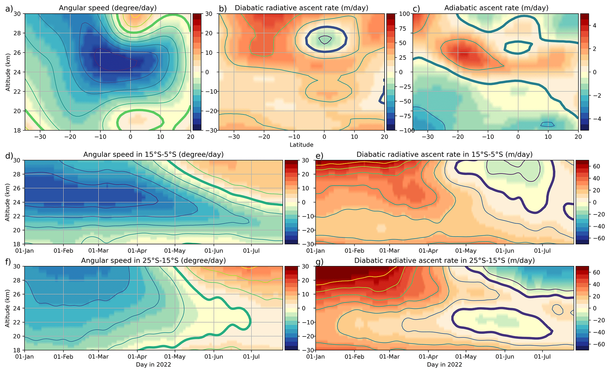
Figure 1 (a) Zonal mean angular rotation speed $\mathit{\omega }=\frac{U}{R_{\mathrm{Earth}}\cos \left(\mathit{\varphi }\right)}$ from ERA5, averaged between 15 January 2022 and 15 March 2022 (in ${}^{\circ }{\mathrm{d}}^{-\mathrm{1}}$). (b) Same as (a) for the diabatic ascent rate calculated from the total all-sky ERA5 heating rate (in m d⁻¹). (c) Same as (a) for the adiabatic ascent rate due to motion of the isentropic surfaces with respect to the geopotential surfaces (in m d⁻¹). (d) Daily zonal and altitude band average angular speed between 15 and 5^∘ S as a function of time (in ${}^{\circ }{\mathrm{d}}^{-\mathrm{1}}$). (e) Same as (d) for the diabatic ascent (in m  d⁻¹). (f)–(g) Same as (d)–(e) for the latitude band between 25 and 15^∘ S.

Figure 2 shows that after an initial rapid meridional dispersion in the first days after the eruption (Khaykin et al., 2022), the aerosol and water plume stay mostly confined within the latitude band 35^∘ S–20^∘ N until June when wave activity increases and evolve slowly in the zonal mean. By mid-February, aerosols and water vapour have already spread through all longitudes (Khaykin et al., 2022, and Fig. 6 below). The Ozone Mapping and Profiler Suite Limb Profiler (OMPS-LP) extinction ratio increases in time at the core of the cloud and reaches a maximum in mid-April. The simultaneous increase of the Cloud-Aerosol Lidar with Orthogonal Polarization (CALIOP) scattering ratio suggests particle growth. The Microwave Limb Sounder (MLS) water vapour distribution initially coincides with that of the aerosols, but the distributions progressively move apart vertically (see also Schoeberl et al., 2022) due to the sedimentation of the aerosols. By early June, aerosols and moisture appear fully separated below and above 25 km, respectively.

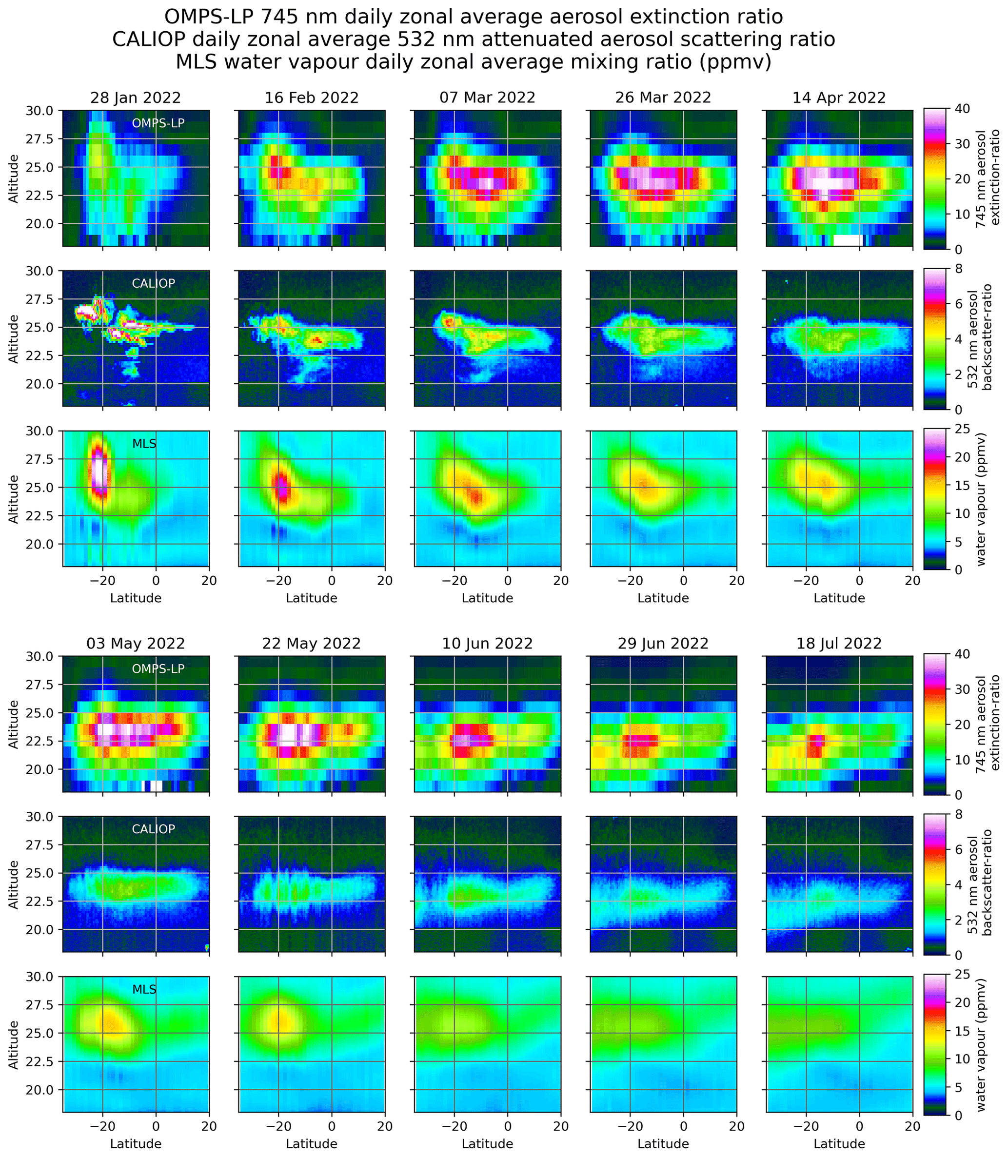
Figure 2 Series of daily zonal averages over all available orbits from three satellites measuring aerosols and water vapour (Appendix A1.3, A1.1 and A1.4). The series is shown in two consecutive blocks of three rows. Upper row: OMPS-LP 745 nm aerosol extinction ratio. Middle row: CALIOP 532 nm aerosol attenuated backscatter ratio. Lower row: MLS water vapour (in ppmv). Days from 28 January 2022 to 16 July 2022 with 19 d step.

The plume vertical motion (Appendix A3) is analysed (Fig. 3) for two latitude bands and the apparent aerosol radius is estimated by interpreting the aerosol plume motion as a fall speed of the scattering particles. The descent of aerosols is separated into two subsequent phases. For the first phase, lasting until about 20 February, Fig. 3a–d show a fast descent in the two latitude bands, which would imply unrealistically large aerosol sizes (Fig. 3e). During this phase, the water vapour follows the aerosol downward motion. Sellitto et al. (2022) (S2022 hereafter) explain this behaviour by the cooling effect of water vapour infrared emission, which is strong as long as the water vapour is concentrated and is located well above its neutral radiative level. Sedimentation is then a secondary effect.

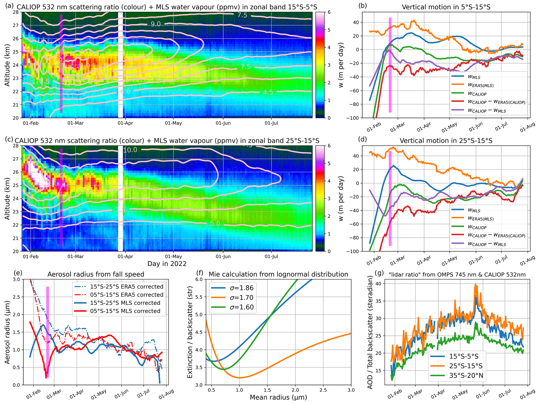
Figure 3 Panels (a) and (c) show zonal and latitude band averages as a function of time for CALIOP 532 nm scattering ratio (colour) and MLS water vapour (contours, ppmv) for the 15–5^∘ S and 25–15^∘ S latitude bands, respectively. Panels (b) and (d) show vertical motions for the same two latitude bands: W_CALIOP for aerosol plume and W_MLS for water vapour plume deduced from (a) and (c) (Appendix A3), W_ERA5(MLS) for ERA5 ascent rate (Appendix A2) at the location of the MLS plume, and W_CALIOP−W_ERA5(CALIOP) and W_CALIOP−W_MLS for the CALIOP sedimentation speed estimated, respectively, with respect to the ERA5 ascent rate and the MLS water ascent rate (Appendix A3). (e) Aerosol radius deduced from the aerosol sedimentation speed interpreted as an aerosol fall speed and using Eq. (9.42) of Seinfeld and Pandis (2016). The dashed lines show the estimate for the ERA5 correction, which is applicable after May when the aerosol and moist layers are separated and the water vapour cooling has ceased, and the solid lines show the estimate for the MLS correction, which is valid as long as the aerosol and moist layers overlap (Appendix A3). (f) Ratio of the theoretical 745 nm aerosol extinction and 532 nm aerosol backscatter cross sections, calculated using a Mie code (see Appendix A4) with three values of the standard deviation σ. (g) Ratio of the 745 nm OMPS LP aerosol optical depth and 532 nm CALIOP integrated attenuated backscatter, both over the vertical range 18 to 30 km. The curves are shown for the same latitude bands as in (a) and (c) and for the 35^∘ S–20^∘ N band that also encompasses the periphery of the aerosol plume. In (a)–(e), a vertical line is drawn on 20 February to indicate the separation between the two phases of the vertical motion as discussed in Sect. 2. During the last third of May, both OMPS LP and CALIOP are perturbed by the intensified solar activity, and the peak seen in panel (g) at such dates must be considered as spurious.

In the second phase, after 20 February, the diluted water vapour is ascending but is still producing a cooling, detected by the departure of its ascent rate from the ERA5 ascent rate (Appendix A2), especially in the 25–15^∘ S band, which persists until June (see also Schoeberl et al., 2022; Coy et al., 2022), where it eventually vanishes as water vapour gets too diluted to produce significant cooling. The estimated sedimentation rate of the scattering aerosols and the corresponding particle radius (Appendix A3) suggest (Fig. 3e) that the aerosol particle size grows up to about 1.4 µm in April–May and starts shrinking in May–June in the 15–5^∘ S band, whereas it stays near 1 µm until June before shrinking in the 25–15^∘ S band.

The extinction-to-backscatter ratio, obtained by combining OMPS-LP and CALIOP data (Fig. 3g), exhibits a growth followed by a decay, which are qualitatively consistent with the aerosol size evolution (Fig. 3g) and the expected behaviour of the ratio (Fig. 3f) in the 1–2 µm size range. Considering the saturation and decay of the extinction (Fig. 2), and the progressive vertical separation of aerosols and moisture, we suggest that the initial growth of the particles was by hygroscopic growth until April, where the extinction culminates, and was followed by coagulation over April–May and then by a decay due to evaporation as the ambient air gets drier, and the aerosol plume is diluted. Coagulation and evaporation are obviously not exclusive, and their competition depends on the ambient conditions that vary over space and time (Hamill et al., 1977). It is also apparent from Fig. 2 that the moist layer is less confined than the aerosol layer and extends in latitude beyond the limits of the figure. The extinction-to-backscatter ratio is also smaller on the periphery of the aerosol plume (Fig. 3g). Therefore, we expect evaporation of the transported sulfate aerosols to occur at such latitudes.

3 Inferred composition of the plume

We now consider the history of the aerosol composition of the plume. The sequence in Fig. 4a–d shows, in agreement with Carr et al. (2022), S2022 and Khaykin et al. (2022), that the ash and ice cloud (brown and deep blue) is rapidly removed within the first day following the eruption, likely via sedimentation of large ice particles which condensed water in excess of the saturated profile up to 35 km on 15 January (Khaykin et al., 2022). Taha et al. (2022) mention that ash is missing in the plume on 17 January from UV satellite observations. What emerges on the west side are two greenish clouds (C1 and C2 on Fig. 4b–d) without any hint of ash (ash would appear as yellow/reddish) in a composite RGB product, denoted as RGB-Ash. The CALIOP cross section through these clouds (Fig. 4e–f) shows a high scattering ratio without depolarization and is hence indicative of predominantly small spherical particles. The two clouds C1 and C2 are well separated in altitude. A few days later, the Light Optical Aerosol Counter flight and ground lidar observations, both from La Réunion, confirm this by showing submicron size, mainly non-absorbing, particles (Kloss et al., 2022; Baron et al., 2022).

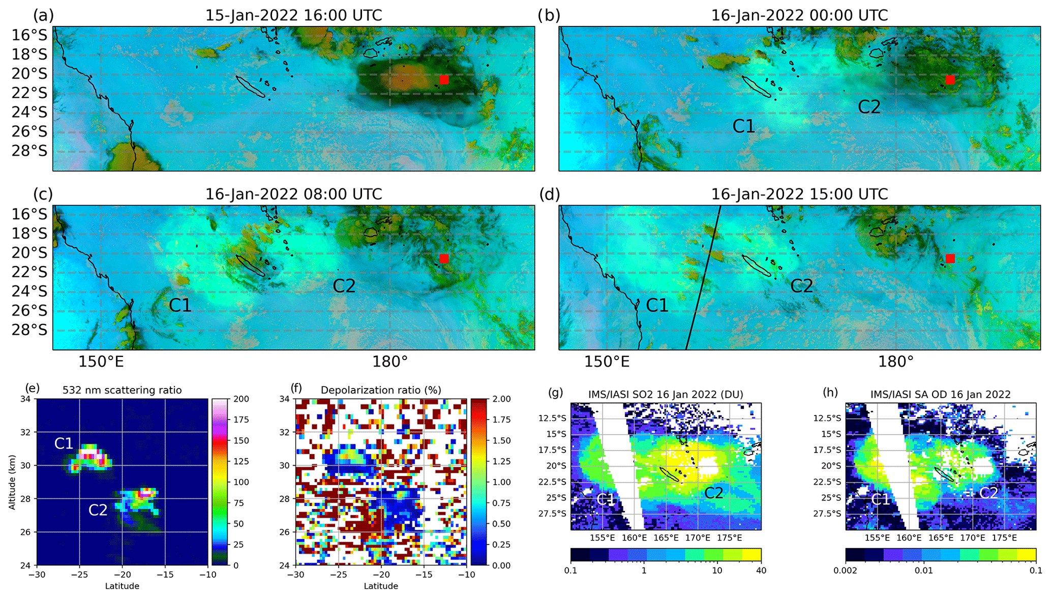
Figure 4 (a)–(d) RGB-Ash composite (see Appendix A1.6) from Himawari-8 at four selected times during the first day and half following the eruption. The red square denotes the location of the volcano. This product allows us to qualitatively distinguish thick ash plumes or ice clouds (brown), thin ice clouds (dark blue) and sulfur-containing plumes (green). Mixed ash-/sulfur-containing volcanic species would appear in reddish and yellow shades. (e) CALIOP 532 nm backscatter ratio at 15:08 UTC along the orbit track shown in panel (d). (f) 532 nm depolarization ratio (orthogonal channel/total) for the same orbit. (g)–(h) SO₂ and SA optical depth from IMS on 16 January 2022 for two night orbits crossing the Equator at 10:26 UTC (right swath) and 12:08 UTC (left swath). The two sulfur clouds produced by the eruption are marked as C1 and C2 in all panels where they are visible but (f).

A further source of information is the Infrared/Microwave Sounder (IMS) retrieval (Appendix A1.2) of SO₂ column and sulfate aerosols (SA) optical depth. Figure 4g–h show that the conversion to sulfates started immediately after the eruption, with an SA optical depth reaching 0.1 one day after the eruption, suggesting that the two clouds seen by CALIOP are composed of almost pure sulfate droplets. The fast conversion of SO₂ to sulfate aerosols is also discussed by S2022 and Zhu et al. (2022), using observations and chemical/transport modelling, respectively. The presence of a significant amount of gas sulfates is not expected under the ambient conditions of the plume (Hamill et al., 1977; Tsagkogeorgas et al., 2017).

A period of 4 d later (Fig. 5b), the two clouds are still separated but have elongated under the zonal shear forming a pair of long strips. Comparing Fig. 5a and b makes it apparent that the conversion to sulfates is almost complete in the western strip generated from C1, while it is incomplete in the eastern strip generated from C2. S2022 show that the western cloud C1 is much moister than the eastern cloud C2, offering a likely reason for faster conversion, as also discussed by Zhu et al. (2022). A cloud C3 of almost pure SO₂ is located between Australia and Indonesia (Fig. 5a), at lower altitudes than the other two clouds, as inferred from its low travelling angular speed. Comparing the IMS products to RGB-Ash (Fig. 5c) demonstrates that RGB-Ash shows sulfates rather than SO₂ as usually assumed since both C1 and C2 are present, but C3 is absent. The sensitivity of geostationary broadband products, like RGB-Ash, to sulfates is shown by Sellitto and Legras (2016).

Figure 5 (a)–(b) SA optical depth and SO₂ from IMS on 20 January 2022 for three night orbits crossing Equator at 14:06 UTC (right swath), 15:48 UTC (middle swath) and 17:29 UTC (left swath). (c) RGB-Ash composite from Meteosat-8 and Himawari-8 at 16:00 UTC on the same day. (d)–(e) Zonal average SA optical depth and SO₂ from 13 January 2022 to 30 April 2022. (f) CALIOP 532 nm attenuated backscatter integrated between 18 and 30 km from 27 January 2022 to 30 April 2022 (per steradian). The sulfur clouds C1 and C2 in Fig. 4 are now seen as two elongated strips, which are marked in (a)–(b). A third cloud C3 is marked in (a)–(b).

The conversion of remaining SO₂ to sulfates proceeds until SO₂ returns to background conditions by late January (Fig. 5d). The sulfates persist for at least 6 months (Fig. 2), and the comparison of Fig. 5e and f shows that zonal averages of IMS and CALIOP products exhibit very similar patterns. The CALIOP depolarization ratio never exceeds its initial value (Fig. 4f) until July.

4 Circumnavigation and instabilities

Figure 6 shows the circumnavigation of the sulfate plume from a series of SA optical depth maps over 1 month and a half (an extended view until 30 April is provided by the supplemental movie (Appendix B)). Due to the differential rotation, the fastest patches near 5^∘ S caught the slowest by 30^∘ S by mid-February, and the plume filled the whole latitude circle. As time proceeds, the components of the plume kept elongating and mixed together towards a zonal uniformity (see movie).

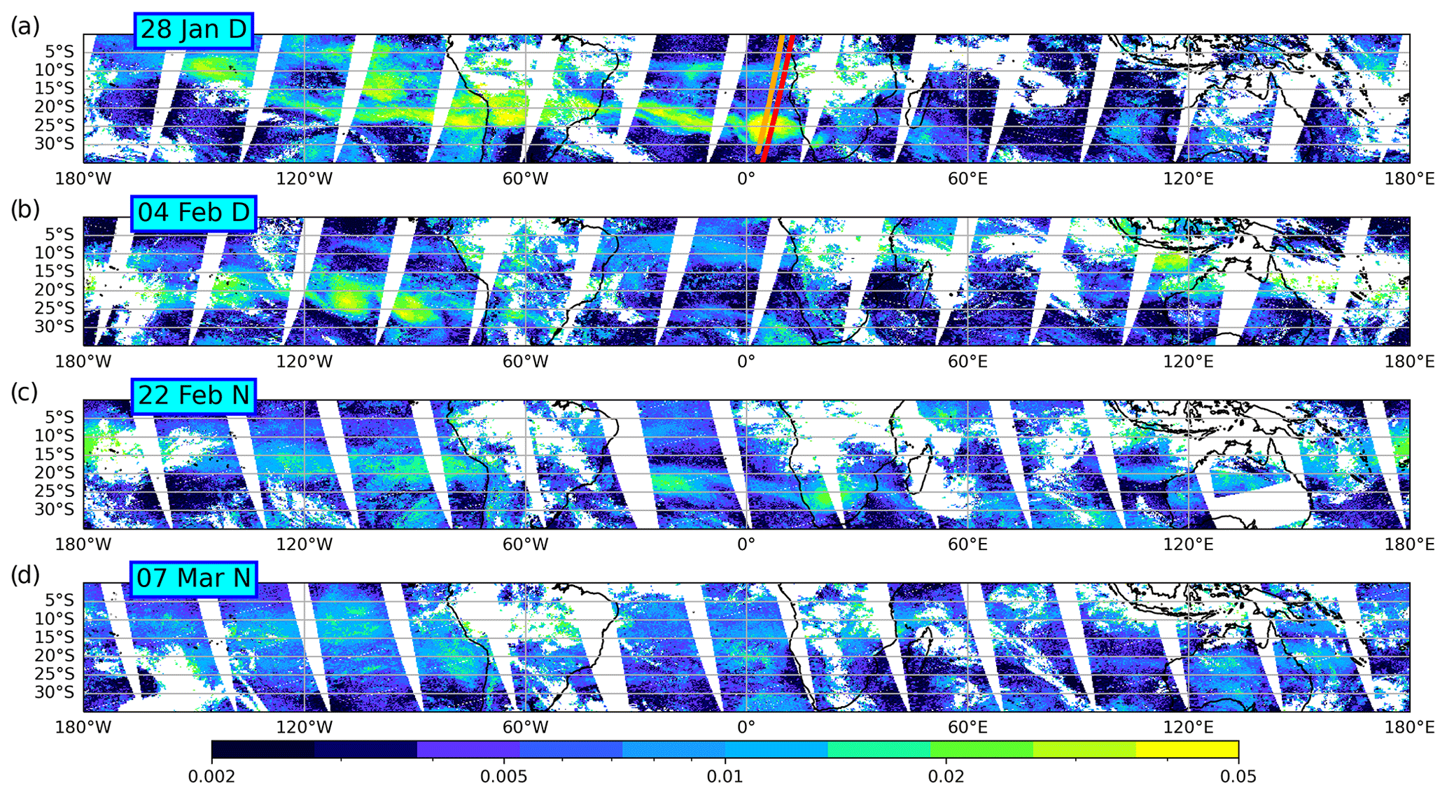
Figure 6 SA optical depth from IMS in the latitude range 0^∘–35^∘ S on four different dates, as indicated. Panels (a)–(b) are drawn for daytime swaths, whereas panels (c)–(d) are drawn for night-time swaths. The time progresses from right to left, and the interval between two adjacent swaths is about 1 h 52 min.

However, Fig. 6 shows a number of localized concentrated patches which persist and keep forming in the plume 1 month after the eruption. Figure 7 investigates the structure of some of them and compares the SA optical depth to the observations from active instruments. Using the Atmospheric Laser Doppler Instrument (ALADIN) (Appendix A1.5), we see (Fig. 7b), on 24 January, an anomalous anticyclonic shear across the highest (28 km) patch at 5^∘ W and 22^∘ S in Fig. 7a, which is part of the western strip defined in Sect. 3. The same pattern is observed on 28 January (Fig. 7c) across a patch near 11^∘ E and 25^∘ S (Fig. 6a), which belongs to the eastern strip. The corresponding CALIOP section (Fig. 7d) exhibits a “jellyfish” pattern with a head at 26 km connected by a tail to lower-altitude patches along an arc of same angular speed (Fig. 1a). This pattern is found repetitively on subsequent CALIOP sections (not shown).

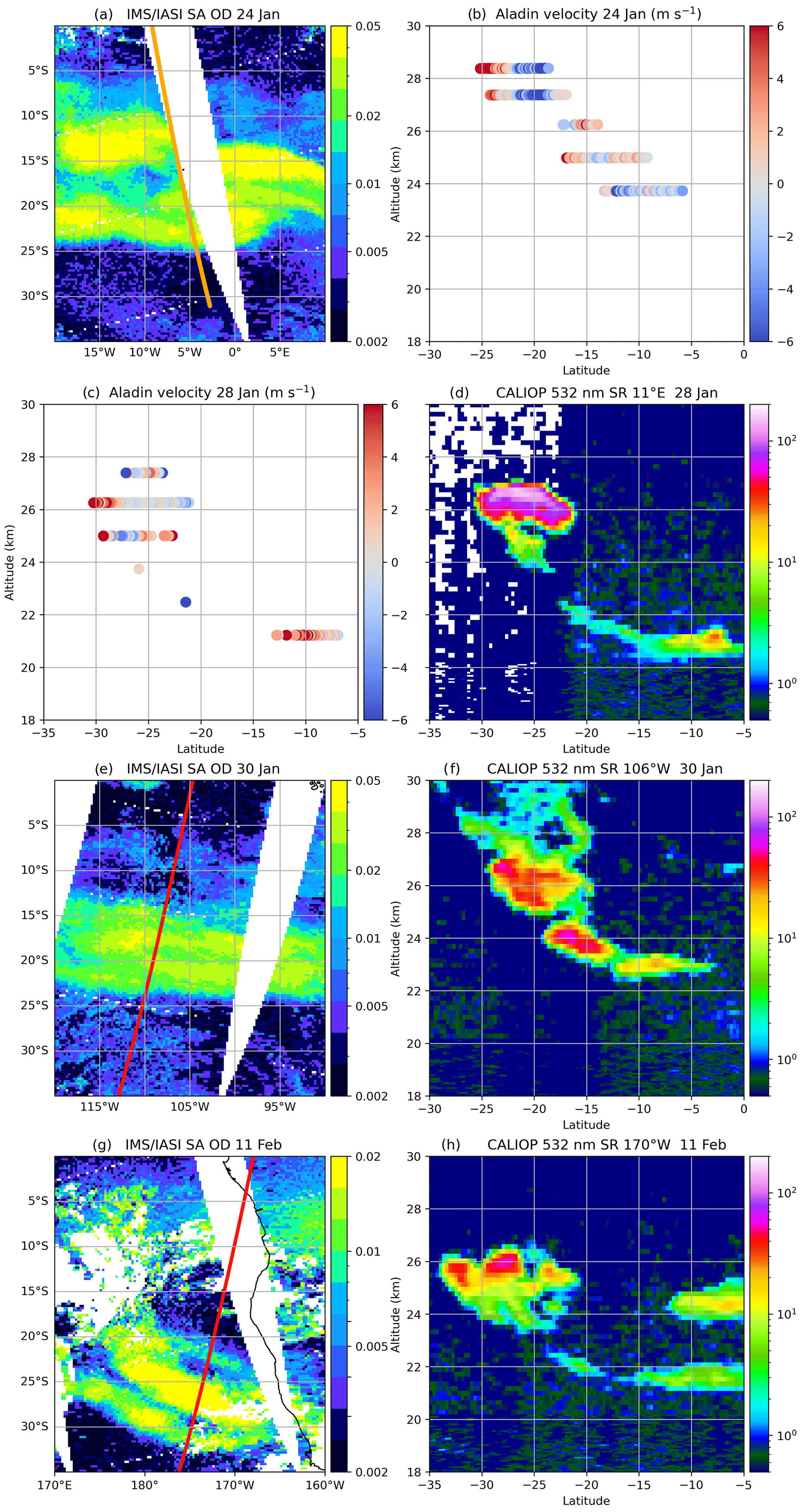
Figure 7 (a) IMS SA optical depth chart on 24 January 2022 near 22:52 UTC for the left swath. (b) ALADIN wind anomaly on 24 January 2022 near 18:36 UTC along the track shown in panel (a). (c) ALADIN wind anomaly near 05:12 UTC on 28 January 2022 along the orange track shown on Fig. 6a within the IASI 08:48 UTC swath on the same day. (d) CALIOP 532 nm scattering ratio on 28 January 2022 near 01:48 UTC along the red track on Fig. 6a. (e) IMS SA optical depth chart on 30 January 2022 near 11:28 UTC for the left swath. (f) CALIOP 522 nm scattering ratio on 30 January 2022 near 09:37 UTC along the red track on panel (e). (g) IMS SA optical depth chart on 11 February near 09:49 UTC for the left swath. (h) CALIOP 522 nm scattering ratio on 11 February near 13:52 UTC along the red track on panel (g).

On 30 January 2022, we are back on the western strip (Fig. 7e), and the corresponding CALIOP section (Fig. 7f) shows filaments overlying the main compact patch that we interpret as a tail left by the fast descent. Again this pattern is repetitively observed on CALIOP sections across the western strip until mid-February where the fast descent halts. The western strip originates from the moister cloud in Fig. 5e that descended faster than the other.

A remarkable feature in the SA optical depth maps is the train of compact elliptical structures linked together by filaments, which is visible all along February and early March in Fig. 6 and the supplemental movie. This peculiar shape is reminiscent of shear-induced instabilities (Juckes, 1995), leading to the formation of a chain of vortices. The suspicion is reinforced by the pattern of a wrapping-up tripolar structure seen near 180^∘ E on 11 February (Fig. 7g) and perfectly captured by CALIOP as a core surrounded by two arms at the same level (Fig. 7h). This comparison also reveals the ability of the IMS product to retrieve small-scale details.

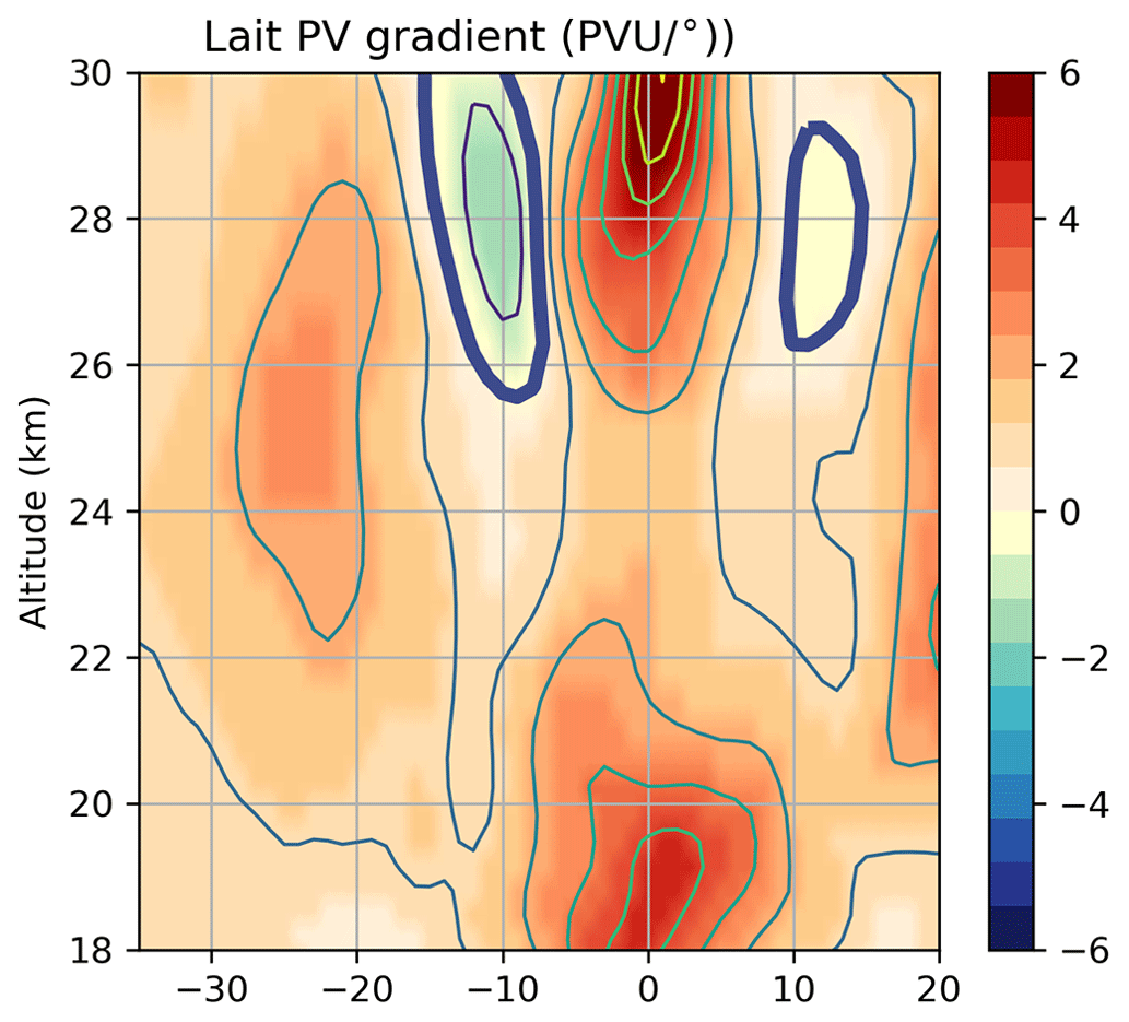
Barotropic shear instability requires a reversal of the meridional gradient of absolute vorticity. The mean flow in ERA5 does not satisfy this criterion. A generalized baroclinic instability requires a reversal of the potential vorticity gradient, but the mean flow again hardly satisfies this criterion at the required altitude of 25 km (Fig. 8). The very fact that the instability produces aerosol patches suggests that they are related to the generation of vorticity. The detection of an anomalous anticyclonic shear across the concentrated patches of the plume by ALADIN (Fig. 7b–c) supports this hypothesis. However, sulfates are poor absorbers, and neither these vortical structures nor their thermal signature have been detected by our present investigation of the ERA5. Therefore, this observation still requires an explanation that we leave for future studies.

Figure 8 Meridional gradient of the zonal and time-averaged Lait PV defined in Appendix A2. The unit is potential vorticity units (PVU) per degree, where 1 PVU = 10⁶ m² Ks⁻¹ kg⁻¹.

5 Discussion and conclusion

The very intense and unusual HTHH eruption generated an intense and unusual stratospheric plume with a huge amount of injected water vapour that remained well above normal 6 months after the eruption. After a fast initial removal of ice and ash, the bulk of the remaining plume consisted of two main clouds between 26 and 32 km travelling westward due to the prevailing phase of the QBO. The ensuing zonal transport dispersed the plume through all longitudes in less than a month (see also Khaykin et al., 2022). The initial SO₂ was fully converted into sulfates in less than 2 weeks under the influence of water vapour. Notice that the absence of detection does not entirely rule out the possible presence of very thin ash as nucleus within sulfate liquid droplets without an optical signature.

The fast initial descent of the upper part of the plume induced by the radiative water vapour cooling has concentrated the aerosols within a fairly narrow layer, about 2 km thick, as seen from CALIOP measurements (Figs. 2 and 5). Within the limit of MLS resolution, the water vapour distribution then coincides with the aerosols. The aerosols later continued subsiding at a slower rate under the effect of gravitational sedimentation, whereas the moist layer entrained by the Brewer–Dobson circulation was simultaneously ascending, so that the two layers progressively separated (as also seen by Schoeberl et al., 2022). The spurious warming in the ERA5 that overlaps the moist layer suggests that radiative cooling by water vapour persists until May (see also Schoeberl et al., 2022; Coy et al., 2022). Although a precise sequencing is difficult without quantitative modelling, it is likely that the sulfate aerosols first grew by hygroscopic growth, then by coagulation and ended by dwindling under evaporation. Our estimation of fall speed and extinction-to-backscatter ratio trends is consistent with a growth up to about 1.4 µm and then a decrease in mean size.

The fast conversion of SO₂ suggests that the initial sulfur injection might have been underestimated. Consistently, S2022 showed that the HTHH eruption produced the largest stratospheric aerosol perturbation since the Pinatubo eruption in 1991 and suggested a large potential for climatic impacts (see also Khaykin et al., 2022). By June, the hemispheric stratospheric aerosol optical depth perturbation of the HTHH plume is twice as large as the peak perturbation of the 2019 Raikoke eruption, and the tropical impact is at least 3 times as large as any volcanic perturbation since Pinatubo 1991 (S2022, Khaykin et al., 2022). As the SO₂ emissions for the Raikoke eruption have been estimated at 1.5 Tg (de Leeuw et al., 2021), we assume this value as the lower limit for the HTHH eruption, 3 times larger than early estimates (Witze, 2022). The young aerosols seem mostly to be made of submicron-sized liquid sulfate particles, then growing to 1.4 µm due to hygroscopic growth and coagulation. The dispersion of the plume questions the magnitude and the duration of the impact. An early estimate of the resulting radiative forcing by S2022 shows that stratospheric aerosol and water vapour perturbations from the eruption may significantly impact the climate system. Given the large greenhouse potential of stratospheric water vapour (e.g. Solomon et al., 2010), it was proposed that the dispersed plume has a net warming effect (S2022), in contrast with the cooling expected from stratospheric aerosols.

Finally, we have shown that the dynamics repetitively generates compact aerosol structures in a process that bears similarities with shear instability and that some structures carry anomalous anticyclonic vorticity. That points to the possible role of such processes in extending the lifetime and the impact of the plume.

Appendix A: Data and methods

A1 Observations

We use data from the following instruments and products.

A1.1 CALIOP

The Cloud-Aerosol Lidar with Orthogonal Polarization (CALIOP) is a spaceborne lidar on board the CALIPSO satellite (Vaughan et al., 2004; Winker et al., 2010). We use the L1 532 nm attenuated backscatter, which is filtered in the horizontal with a median filter of width 102 km. In particular, this filter removes the noise associated with the South Atlantic Anomaly (SAA) in the Earth's magnetic field, which perturbs CALIOP data between 30 and 80^∘ W (Noel et al., 2014). In practice, a limited amount of data are usable in this region and only at night. After filtering, the data are further averaged at a resolution of 34 km for compactness. The other channels are processed in the same way.

Due to solar activity, CALIOP was not operating on 18 January and between 20 and 26 January. Hence, our CALIOP series start on 27 January. We only use night-time data in this work. The molecular backscatter is calculated following Hostetler et al. (2006). For each day, the backscatter ratio is zonally averaged over all available orbits of that day (14 to 15 for a nominal day). The native vertical resolution in the 20–30 km range is 180 m.

A1.2 IMS

The RAL (Rutherford Appleton Laboratory) Infrared/Microwave Sounder (IMS) retrieval core scheme (Siddans, 2019) uses an optimal estimation spectral fitting procedure to retrieve atmospheric and surface parameters jointly from co-located measurements by IASI (Infrared Atmospheric Sounding Interferometer), AMSU (Advanced Microwave Sounding Unit) and MHS (Microwave Humidity Sounder) on MetOp-B spacecraft, using RTTOV-12 (Radiative Transfer for TOVS) (Saunders et al., 2017) as the forward radiative transfer model. The use of RTTOV-12 enables the quantitative retrieval of volcanic-specific aerosols (sulfate aerosol) and trace gases (SO₂). The present paper uses IMS SO₂ and sulfate aerosol observations from its near-real-time implementation. The IMS scheme retrieves the SO₂ in the sensitive region around 1100–1200 cm⁻¹ (in ppbv), assuming a uniform vertical mixing ratio. It retrieves sulfate-specific optical depth at 1170 cm⁻¹ (i.e. the peak of the mid-infrared extinction cross section; Sellitto and Legras, 2016), assuming a Gaussian extinction coefficient profile shape peaking at 20 km altitude, with 2 km full-width half-maximum. The bulk of the spectroscopic information on SO₂ and sulfate aerosols, in the IMS scheme, thus comes from the Infrared Atmospheric Sounding Interferometer (IASI) (Clerbaux et al., 2009). We refer to the two retrieved products as IMS SO₂ and SA optical depth (SA OD in the figure titles) in this work. The data are provided daily on a regular grid with 0.25^∘ resolution in latitude and longitude, with one image collecting the daytime swaths and another collecting the night-time swaths.

A1.3 OMPS-LP

The Ozone Mapping and Profiler Suite Limb Profiler (OMPS-LP) on board the Suomi-NPP satellite provides along-track vertical profiles of aerosol extinction in several visible bands (Loughman et al., 2018; Taha and Loughman, 2020). We use version 2.1 and the 745 nm band, as recommended by Taha et al. (2021). Swaths with non-zero quality flag are discarded. Basically, this filters data polluted by the SAA, but filtered and non-filtered results differ very little in our processing. The molecular extinction is calculated from the same formulas as the CALIOP molecular backscatter but for a change of wavelength. The extinction is averaged daily over all available orbits of that day and after a horizontal interpolation to a latitude grid of 1.1^∘ resolution that corresponds to the mean resolution of OMPS-LP in the considered range of latitudes.

OMPS-LP has a vertical resolution of 1.5 km, which is lower than the vertical resolution of CALIOP. It is also sensitive to the arch effect (Gorkavyi et al., 2021), which tends to shift the apparent bottom of an extended aerosol layer downward by several kilometres.

A1.4 MLS

The Microwave Limb Sounder (MLS) on board NASA's AURA satellite provides along-track vertical profiles of water vapour mixing ratio (Lambert et al., 2015; Schwartz et al., 2020) as well as other trace gases, temperature and cloud ice. We use version 4 without accounting for the quality flag as in Millán et al. (2022). The data are projected and zonally averaged daily onto a fixed-latitude grid of 1.45^∘ resolution in the domain of interest. As they are provided on pressure levels with an approximate vertical resolution of 1.5 km, similar to that of OMPS-LP, they are interpolated to altitudes using the geopotential calculated daily on the ERA5 zonal mean. In order to get estimates of the altitudes by the method described in Appendix A3, the interpolation is done to a resolution of 100 m using a non-oscillating Akima interpolator.

A1.5 ALADIN

The Atmospheric Laser Doppler Instrument (ALADIN) on board the Aeolus satellite is the first spaceborne Doppler wind lidar (Rennie et al., 2020). It is designed to measure wind along the line of sight from the Doppler shift of the 355 nm light emitted by the laser and scattered back by molecules (Rayleigh wind) or aerosols (Mie wind). Horizontal line-of-sight wind is retrieved neglecting the vertical wind component. The anomaly wind is calculated by removing the background wind at the same time and location from ERA5. As the line of sight is perpendicular to the heliosynchronous orbit, the measured component at low latitudes and mid-latitudes is essentially the zonal wind. The ceiling of Aeolus vertical bins can be adjusted and was increased to 30 km in the area of the HTHH plume (30^∘ S–0^∘) a few days after the eruption. We use the Mie product which is of better quality than the Rayleigh product inside the plume (Zuo et al., 2022).

A1.6 RGB-Ash

We use a composite RGB product, denoted as RGB-Ash, that benefits from the sensitivity of the 8.5 µm band of the Advanced Himawari Imager (AHI) and Spanning Enhanced Visible and InfraRed Imager (SEVIRI) on board the geostationary Himawari-8 and Meteosat-8 satellites. The product is based on the EUMETSAT Ash RGB recipe (https://navigator.eumetsat.int/product/EO:EUM:DAT:MSG:VOLCANO/print, last access: 26 May 2020) and uses the brightness temperatures (BT in kelvin) of the three channels: 8.5, 10.4 and 12.3 µm. The recipe for the three colour indexes ranging from 0 to 1 is $R=\left(\mathrm{BT}\right(\mathrm{12.3})-\mathrm{BT}(\mathrm{10.4})+\mathrm{2574})/\mathrm{6}$, $G=\left(\mathrm{BT}\right(\mathrm{10.4})-\mathrm{BT}(\mathrm{8.5})+\mathrm{4})/\mathrm{9}$ and $B=\left(\mathrm{BT}\right(\mathrm{10.4})-\mathrm{243})/\mathrm{60}$. The same recipe is used for both instruments, even if the channels are not strictly identical. This product allows us to qualitatively distinguish thick ash plumes or ice clouds (brown), thin ice clouds (dark blue) and sulfur-containing plumes (green). Mixed ash-/sulfur-containing volcanic species would appear in reddish and yellow shades.

A2 ERA5 reanalysis and meteorological data

We use the European Centre for Medium Range Forecasts ERA5 reanalysis (Hersbach et al., 2020) at 1^∘ × 1^∘  resolution and all the model levels with 6-hourly sampling at 00:00, 06:00, 12:00 and 18:00 UTC. Geopotential, potential temperature and potential vorticity are calculated at full resolution for each time. All the fields are then averaged in longitude and over the four daily samples to provide a daily zonal average. At the stratospheric altitudes which are relevant to this study, the model levels are pure pressure, and therefore the averages are made over isobars.

The total all-sky radiative heating rate is converted into diabatic vertical velocity from the profile of pressure, geopotential and temperature. The motion of the isentropes with respect to the geopotential in the zonal mean is used to define the adiabatic vertical velocity (see Appendix A3).

The ERA5 does not assimilate the anomalous water vapour or the aerosols in the stratosphere and therefore cannot account for their direct radiative effect, either short-wave absorption or longwave absorption and emission. However, it assimilates the induced temperature perturbation if it is large enough to be detected and then reacts to dampen it by longwave radiative relaxation with a timescale of the order of 5 d at 25 km (Lestrelin et al., 2021).

In the present case, the water vapour radiative cooling creates a negative temperature anomaly overlapping the plume (Schoeberl et al., 2022; Coy et al., 2022) that generates a spurious compensating heating rate and exaggerated vertical ascent.

The Lait potential vorticity (LPV) used in Fig. 8 is defined from the Ertel potential vorticity (PV) as

$$\mathrm{LPV}={\left({\displaystyle \frac{\mathrm{600}}{\mathit{\theta }}}\right)}^{\mathrm{4}}\mathrm{PV},$$

where θ is the potential temperature in kelvin.

A3 Vertical motion from CALIOP and MLS

The observed vertical motion is obtained from CALIOP and MLS by applying a second-order Savitzky–Golay filter with a 31 d window to the daily mean vertical location of CALIOP scattering ratio and MLS water vapour, retaining data above 2 and 6 ppmv offsets, respectively. The offset are defined to isolate the aerosol and the water plumes from the background. The 31 d window has been adjusted from several trials with 11, 21, 31 and 41 d as the value beyond which the resulting motion curve was rid of short time fluctuations and did not change any more in shape. This was reached with the 31 d window for MLS and the 21 d window for CALIOP, but for the sake of consistency, we use the 31 d window for both.

The diabatic and adiabatic background vertical velocities are calculated from ERA5 zonal means. The diabatic motion results from the total radiative heating rate $\frac{DT}{Dt}{|}_{\mathrm{RAD}}$ multiplied by $\frac{\mathit{\theta }}{T}\frac{\mathit{\delta }z}{\mathit{\delta }\mathit{\theta }}$, where $(T,\mathit{\theta },z)$ are temperature, potential temperature and geopotential altitude. The adiabatic motion, which is always a small correction, is estimated as $-\frac{\partial \mathit{\theta }}{\partial t}{|}_p\frac{\mathit{\delta }z}{\mathit{\delta }\mathit{\theta }}+\frac{\partial z}{\partial t}{|}_p$, where derivatives are taken at constant pressure p. The calculations are made by centred finite differences on the model grid, which is in pure pressure in the considered altitude range.

Two correction methods are applied to the observed descent of aerosols from CALIOP in order to estimate the sedimentation velocity with respect to the air. In the first method, the ascent of the water vapour plume seen by MLS is used as an estimate of air motion, and in the second method, the sum of diabatic and adiabatic ERA5 vertical velocities provides this estimate. Then this air motion is added to the aerosol descent rate to estimate the sedimentation velocity. The first method is applicable to the period during which the aerosol and water vapour distributions overlap, and the water vapour cooling perturbs the heating rate estimate of ERA5. The second method applies at a later stage when the aerosol and water vapour distributions are well separated, and the radiative effect of water vapour has been defeated by dilution. As the boundary between these two regimes cannot be defined accurately, we show the results of the two methods.

The scattering aerosol radius is then estimated using Stokes' fall speed formula for small particles (Seinfeld and Pandis, 2016).

A4 Mie calculations

The theoretical extinction-to-backscatter ratio for the plume has been calculated using the Python-based miepython Mie code, available at https://miepython.readthedocs.io/en/latest/ (last access: 20 May 2022). The extinction and backscatter coefficients have been estimated at 750 and 532 nm, respectively, to simulate OMPS and CALIOP observations. Typical sulfate aerosol refractive indices have been considered, with the assumption of very weakly absorbing particles (based on the results of Kloss et al., 2022). Lognormal size distributions with varying standard deviation are simulated, to study how this ratio changes with radius.

Appendix B: IMS animation

The animation in the Supplement https://doi.org/10.5281/zenodo.7242467 (Legras et al., 2022) shows the IMS SA optical depth product for all daytime and night-time orbits of each day between 13 January and 30 April 2022. The indicated times are those of the intersection of the orbits with the Equator. When two orbit swaths overlap, the crossing time of the overlapped orbit is indicated in red. Missing orbits are blanked out. Several days are missing entirely between 8 and 14 March.