Quantifying the drivers of surface ozone anomalies in the urban areas over the Qinghai-Tibet Plateau

Improved knowledge of the chemistry and drivers of surface ozone over the Qinghai-Tibet Plateau (QTP) is significant for regulatory and control purposes in this high-altitude region in the Himalayas. In this study, we investigate the processes and drivers of surface ozone anomalies (defined as deviations of ozone levels relative to their seasonal means) between 2015 and 2020 in urban areas over the QTP. We separate quantitatively the contributions of anthropogenic emissions and meteorology to surface ozone anomalies by using the random forest (RF) machine-learning model-based meteorological normalization method. Diurnal and seasonal surface ozone anomalies over the QTP were mainly driven by meteorological conditions, such as temperature, planetary boundary layer height, surface incoming shortwave flux, downward transport velocity and inter-annual anomalies were mainly driven by anthropogenic emission. Depending on region and measurement hour, diurnal surface ozone anomalies varied over −27.82 to 37.11 µg m⁻³, whereas meteorological and anthropogenic contributions varied over −33.88 to 35.86 µg m⁻³ and −4.32 to 4.05 µg m⁻³ respectively. Exceptional meteorology drove 97 % of surface ozone non-attainment events from 2015 to 2020 in the urban areas over the QTP. Monthly averaged surface ozone anomalies from 2015 to 2020 varied with much smaller amplitudes than their diurnal anomalies, whereas meteorological and anthropogenic contributions varied over 7.63 to 55.61 µg m⁻³ and 3.67 to 35.28 µg m⁻³ respectively. The inter-annual trends of surface ozone in Ngari, Lhasa, Naqu, Qamdo, Diqing, Haixi and Guoluo can be attributed to anthropogenic emissions in 95.77 %, 96.30 %, 97.83 %, 82.30 %, 99.26 % and 87.85 %, and meteorology in 4.23 %, 3.70 %, 2.17 %, 3.19 %, 0.74 % and 12.15 % respectively. The inter-annual trends of surface ozone in other cities were fully driven by anthropogenic emission, whereas the increasing inter-annual trends would have larger values if not for the favorable meteorological conditions. This study can not only improve our knowledge with respect to spatiotemporal variability of surface ozone but also provide valuable implications for ozone mitigation over the QTP.

1 Introduction

The Qinghai-Tibet Plateau (QTP) (27–45^∘ N, 70–105^∘ E), with an average altitude of 4000 m a.s.l. (above sea level), is the highest plateau in the world. It is known as the “Roof of the World” and the “Third Pole” (Qiu, 2008; Yang et al., 2013; Yin et al., 2017). The QTP has an area of approximately 2.5×10⁶ km² and accounts for about one quarter of China's territory (Duo et al., 2018). The QTP is the source region of five major rivers in Asia, i.e., the Indus, Ganges, Brahmaputra, Yangtze and Yellow rivers, which provide water resources to more than 1.4 billion people (Immerzeel et al., 2010). The QTP has been verified to be a critical region for regulating Asian monsoon climate and hydrological cycle, and it is thus an important ecological barrier for the whole of Asia (Loewen et al., 2007; Yanai et al., 1992). The QTP has long been regarded as a pristine region owing to its low population and industrial levels (Zhu et al., 2013). Because of its unique features of landform, ecosystem and monsoon circulation pattern, the QTP has been regarded as a region that is sensitive to anthropogenic impact, and is referred to as an important indicator of regional and global climate change (Qiu, 2008). The exogenous and local atmospheric pollutants have the potential to accelerate the melting of glaciers, damage air quality, water sources and grasslands, and threaten climate on regional and global scales (Yin et al., 2017; X. F. Yin et al., 2019; Sun et al., 2021d; Pu et al., 2007; Kang et al., 2016). Therefore, improved knowledge of the evolutions and drivers of atmospheric pollutants in the QTP is of great importance for understanding the local ecological situation and formulating regulatory policies.

Surface ozone (O₃) is a major air pollutant that threatens human health and vegetation growth (Jerrett et al., 2009; Yin et al., 2021b). Surface ozone over the QTP is generated either from its local anthropogenic and natural precursors such as nitrogen oxides (NO_x), volatile organic compounds (VOCs) and carbon monoxide (CO) via a chain of photochemical reactions or transported from long-distance regions by downwelling from the stratosphere. Surface ozone level is sensitive to local emissions, meteorological conditions and transport. Meteorological conditions affect surface ozone level indirectly through changes in natural emissions of its precursors or directly via changes in wet and dry removal, dilution, chemical reaction rates and transport flux. Emissions of air pollutants affect surface ozone level by perturbing the abundances of hydroperoxyl (HO₂) and alkylperoxyl (RO₂) radicals, which are the key atmospheric constituents in the formation of ozone. Some previous studies have presented the variability and analyzed qualitatively the drivers of surface ozone over the QTP at a specific site or region (Xu et al., 2016; X. Yin et al., 2019; Yin et al., 2017; Zhu et al., 2004). However, none of these studies has quantitatively separated the contributions of anthropogenic emission and meteorology. Separation of anthropogenic and meteorological drivers is very important as it conveys to us exactly which processes drive the observed ozone anomaly and therefore the correct conclusions can be drawn on whether an emission mitigation policy is effective.

Chemical transport models (CTMs) are widely used to evaluate the influences of meteorology and anthropogenic emission on atmospheric pollution levels (Hou et al., 2022; Sun et al., 2021a; Yin et al., 2020; Yin et al., 2019). However, there are significant uncertainties in the emission inventories and in the models themselves, and shutting down an emission inventory in CTMs may cause a large nonlinear effect, which inevitably influences the accuracy, performance and efficiency of CTMs (Vu et al., 2019; Zhang et al., 2020). Mathematical and statistical models such as the multiple linear regression (MLR) model and general additive models (GAMs) have also been used in many studies to quantify the influence of meteorological factors (Li et al., 2019; K. Li et al., 2020; Yin et al., 2021a; Yin et al., 2022; Zhai et al., 2019).

Machine learning (ML) is a well-known field that has been developing rapidly in recent years. ML is a fusion of statistics, data science and computing that experiences use across a very wide range of applications (Grange et al., 2018). Unlike most ML models, such as artificial neural networks, whose working mechanisms are hard to understand, the random forest (RF) model is not a “black-box” method, its prediction process can be explained, investigated and understood (Gardner and Dorling, 2001; Grange et al., 2018; Grange and Carslaw, 2019; Shi et al., 2021). Recently, the RF model-based meteorological normalization technique has been proposed and used to decouple the influence of meteorology on atmospheric pollution. For example, Vu et al. (2019) have used this technique to demonstrate that the clean air action plan implemented in 2013 was highly effective in reducing the anthropogenic emissions and improving air quality in Beijing. Shi et al. (2021) have used this technique to quantitatively evaluate changes in ambient NO₂, ozone, and PM_2.5 concentrations arising from these emission changes in 11 cities globally during the COVID-19 lockdowns.

Figure 1 Geolocations of each city over the Qinghai-Tibet Plateau (QTP). The base map of the figure was created using the Basemap package in Python.

In this study, we investigate the evolutions, implications and drivers of surface ozone anomalies (defined as deviations of ozone levels relative to their seasonal means) from 2015 to 2020 in the urban areas over the QTP. Compared with previous studies, which focused on surface ozone over the QTP, this study involves a larger area and a longer time span. Most importantly, this study separates quantitatively the contributions of anthropogenic emission and meteorology to surface ozone anomalies by using the RF model- based meteorological normalization method. This study can not only improve our knowledge with respect to spatiotemporal variability of surface ozone but also provide valuable implication for ozone mitigation over the QTP. We introduce detailed descriptions of the surface ozone and meteorological field dataset in Sect. 2. The method for separating contributions of meteorology and anthropogenic emission is presented in Sect. 3. Section 4 analyzes spatiotemporal variabilities of surface ozone from 2015 to 2020 in each city over the QTP. The performance of the RF model used for surface ozone prediction over the QTP is evaluated in Sect. 5. We discuss the implications and the drivers of surface ozone anomalies from 2015 to 2020 in each city over the QTP in Sect 6. We conclude this study in Sect. 7.

2 Data sources

2.1 Surface ozone data

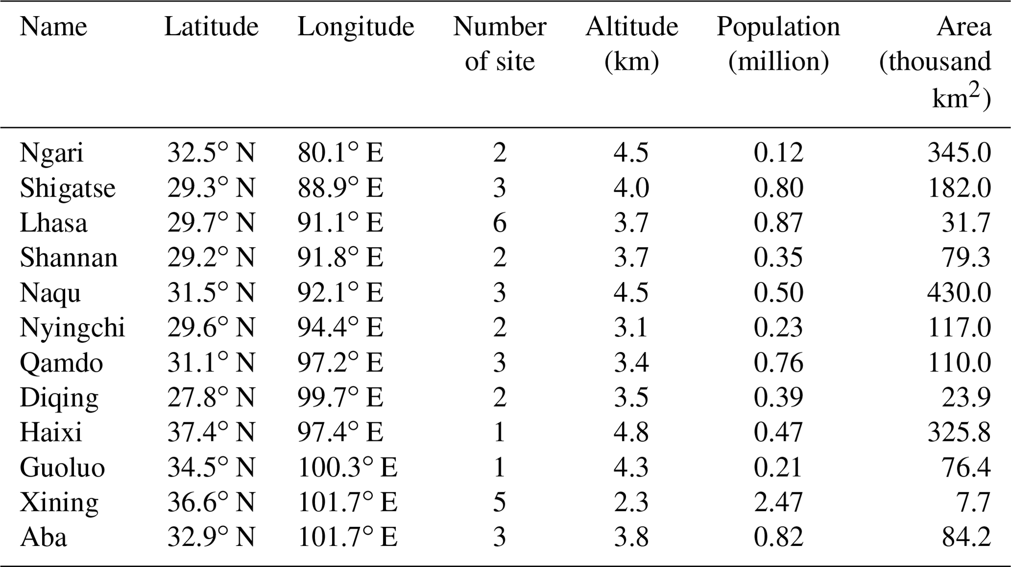
The QTP covers an area of 2.5 million square meters and has a population of around 3 million, with most of them living in several cities. During the in-depth study of the atmospheric chemistry over the Tibetan Plateau, @Tibet field campaign, ozone photochemistry and its roles in ozone budget are of great interest in both background atmosphere and in QTP urban areas. The former represents the influence of anthropogenic emission and cross-boundary transport on the nature cycle of ozone in pristine atmosphere. The latter represents not only the upper limit of ozone photochemistry contribution to its budget, also demanding knowledge for the sake of ozone pollution management. As illustrated in Fig. 1, the QTP (latitude range: 26^∘00^′–39^∘47^′, longitude range: 73^∘19^′–104^∘47^′) covers the Kunlun Mountain, the A-erh-chin Mountain and the Qilian Mountain in the north, the Pamir Plateau and the Karakorum Mountains in the west, the Himalayas in the south, and the Qinling Mountains and the Loess Plateau in the east. The 12 cities are the most populated areas over the QTP. All these cities except for Aba and Diqing are located in the Tibet or Qinghai provinces. Aba and Diqing are in the Sichuan and Yunnan provinces respectively. The area of these cities ranges from 7.7 to 430 thousand km², the altitude ranges from 2.3 to 4.8 km a.s.l. and the population ranges from 0.12 to 2.47 million. The residents within the 12 cities number about 3.85 million and account for about 51 % of the population over the QTP.

Table 1 Geolocations of each city over the QTP. Population statistics are available from the 2020 nationwide population census issued by the National Bureau of Statistics of China.

Hourly surface ozone data in the urban areas over the QTP are available from the China National Environmental Monitoring Center (CNMEC) network (http://www.cnemc.cn/en/, last access: 26 November 2021). The CNMEC network-based ozone measurements have been widely used in many studies for the evaluation of regional atmospheric pollution and transport over China (Lu et al., 2019a, 2020, 2021; Sun et al., 2021c, d; Yin et al., 2021a, b, 2022). The CNEMC network has deployed 33 measurement sites in 12 cities over the QTP (Table 1). The number of measurement sites in each city varies from 1 to 6. All surface ozone time series at each measurement site are provided by active differential absorption ultraviolet (UV) analyzers. For all the 33 measurement sites, hourly surface ozone data since 2015 are available. We first removed unreliable measurements at all measurement sites in each city by using the filter criteria following our previous studies (Lu et al., 2018, 2020; Sun et al., 2021b, d; Yin et al., 2021a, b), then averaged all measurements in each city to generate a city representative dataset. All investigations in this study are performed on such a city representative basis.

The filter criteria can be summarized as follows. Hourly observed data points were first transformed into Z scores via Eq. (1) and the observed data were then removed if the corresponding Z_i value met one of the following conditions: (1) Z_i is larger or smaller than the previous one (Z_i−1) by 9 ($|Z_i-Z_{i-\mathrm{1}}|>\mathrm{9}$), (2) the absolute value of Z_i is greater than 4 ($\left|Z_i\right|>\mathrm{4}$) or (3) the ratio of the Z value to the third-order center moving average is greater than 2 $\left(\frac{\mathrm{3}{Z}_i}{Z_{i-\mathrm{1}}+Z_i+Z_{i+\mathrm{1}}}>\mathrm{2}\right)$.

$$\begin{array}{}\text{(1)}& z_k={\displaystyle \frac{x_k-u_k}{{\mathit{\sigma }}_k}},\end{array}$$

where u_k and σ_k are the average and 1σ standard deviation (SD) of x_k, and z_k is the pre-processed value for parameter x_k.

2.2 Meteorological data

Meteorological fields used in this study are from the Modern-Era Retrospective analysis for Research and Applications Version 2 (MERRA-2) dataset (Gelaro et al., 2017). The MERRA-2 dataset is produced by the NASA Global Modeling and Assimilation Office and it can provide time series of many meteorological variables with a spatial resolution of $\mathrm{0.5}{}^{\circ }\times \mathrm{0.625}{}^{\circ }$ (GMAO, 2022). The boundary layer height and surface meteorological variables are available per hour and other meteorological variables are available every 3 hours. It has been verified that the MERRA-2 meteorological fields over the QTP are in good agreement with the observations (Wang and Zeng, 2012; Xie et al., 2017). This MERRA-2 dataset has been extensively used in evaluations of regional atmospheric pollution formation and transport over China (Carvalho, 2019; Kishore Kumar et al., 2015; Song et al., 2018; Zhou et al., 2017; Li et al., 2019; K. Li et al., 2020; Yin et al., 2022; Zhai et al., 2019).

3 Methodology

3.1 Quantifying seasonality and inter-annual variability

We quantify the seasonality and inter-annual variability of surface ozone from 2015 to 2020 in each city over the QTP by using a bootstrap resampling method. The principle of such a bootstrap resampling method was described in detail in Gardiner et al. (2008). Many studies have verified the robustness of Gardiner's methodology in modeling the seasonality and inter-annual variabilities of a suite of atmospheric species (Sun et al., 2020; Sun et al., 2018, 2021a, b, d). In this study, we used a second Fourier series plus a linear function to fit surface ozone monthly mean time series from 2015 to 2020 over the QTP. The usage of measurements on monthly basis can improve the fitting correlation and lower the regression residual. As a result, the relationship between the measured and bootstrap resampled surface ozone monthly mean time series can be expressed as

$$\begin{array}{}\text{(2)}& {\displaystyle }\begin{array}{rl}V(t,b)& =b_{\mathrm{0}}+b_{\mathrm{1}}t+b_{\mathrm{2}}\cos \left({\displaystyle \frac{\mathrm{2}\mathit{\pi }t}{\mathrm{12}}}\right)+b_{\mathrm{3}}\sin \left({\displaystyle \frac{\mathrm{2}\mathit{\pi }t}{\mathrm{12}}}\right)\\ & +b_{\mathrm{4}}\cos \left({\displaystyle \frac{\mathrm{4}\mathit{\pi }t}{\mathrm{12}}}\right)+b_{\mathrm{5}}\sin \left({\displaystyle \frac{\mathrm{4}\mathit{\pi }t}{\mathrm{12}}}\right)\end{array}\text{(3)}& {\displaystyle }F(t,a,b)=V(t,b)+\mathit{\epsilon }\left(t\right),\end{array}$$

where $F(t,a,b)$ and V(t,b) represent the measured and fitted surface ozone time series respectively. The parameters b₀–b₅ contained in the vector b are coefficients obtained from the bootstrap resampling regression with V(t,b). The b₀ is the intercept, the b₁ is the annual growth rate and $b_{\mathrm{1}}/b_{\mathrm{0}}$ is the inter-annual trend discussed below. The parameters b₂–b₅ describe the seasonality, t is the measurement time in the month elapsed since January 2015, and ε(t) represents the residual between the measurements and the fitting results. The autocorrelation in the residual can increase the uncertainty in calculation of inter-annual trend. In this study, we have followed the procedure of Santer et al. (2008) and included the uncertainty arising from the autocorrelation in the residual.

3.2 Random forest model

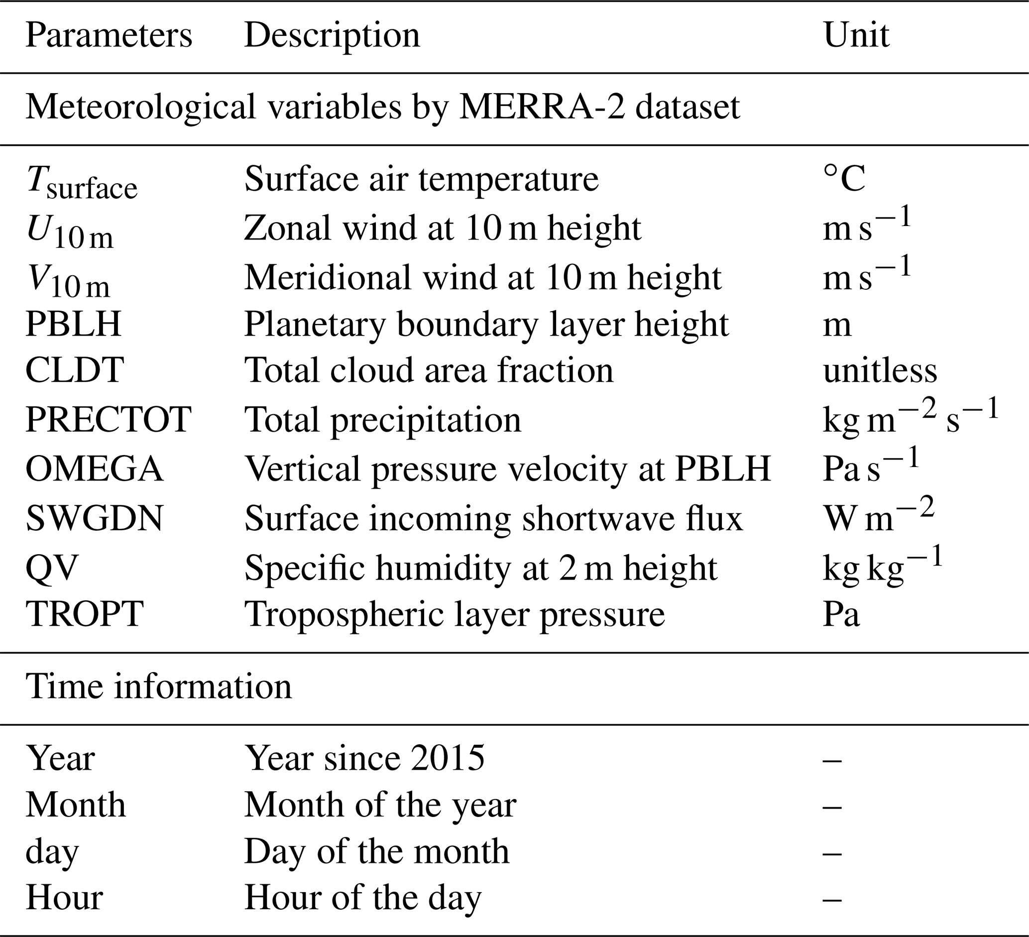
We have established a decision tree-based random forest (RF) machine-learning model to describe the relationships between hourly surface ozone concentrations (response variables) and their potential driving factors (predictive variables) in the urban areas over the QTP. As summarized in Table 2, predictive variables used in this study include time variables such as year 2015 to 2020, month 1 to 12, day of the year from 1 to 365, hour of the day from 0 to 23 and meteorological parameters such as wind, temperature, pressure, cloud fraction, rainfall, vertical transport, radiation and relative humidity. These time variables were selected as proxies for emissions as pollutant emissions vary by the time of day, day of the week and season (Grange et al., 2018).

Table 2 List of predictive variables fed into the RF model.

The detailed descriptions of RF machine-learning model can be found in Breiman (2001). Briefly, the RF model is an ensemble model consisting of hundreds of individual decision tree models. Each individual decision tree model uses a bootstrap aggregating algorithm to randomly sample response variables and their predictive variables with a replacement from a training dataset. In this study, a single regression decision tree is grown in different decision rules based on the best fitting between surface ozone measurements and their predictive variables. The predictive variables are selected randomly to give the best split for each tree node. The predicted surface ozone concentrations are given by the final decision as the outcome of the weighted average of all individual decision trees. By averaging all predictions from bootstrap samples, the bagging process decreases variance and thus helps the model to minimize overfitting.

Figure 2 Flowchart for separation of meteorology and anthropological contributions.

As shown in Fig. 2, the whole dataset was randomly divided into (1) a training dataset to establish the RF model and (2) a testing dataset (not included in model training) to evaluate the model performance. The training dataset was randomly selected from 70 % of the whole data and the remaining 30 % was taken as the testing dataset. The hyperparameters for the RF model in this study were configured following those in Vu et al. (2019) and Shi et al. (2021) and are summarized as follows: the maximum tree of a forest is 300 (n_tree = 300), the number of variables for splitting the decision tree is 4 (mtry = 4) and the minimum size of terminal nodes is 3 (min_node_size = 3). As the meteorological variables differ in units and magnitudes, which could lead to unstable performance of the model, we therefore uniformized all meteorological variables via Eq. (1) before using them in the RF model. This pre-processing procedure can also speed up the establishment of the RF model.

3.3 Separation of meteorological and anthropologic contributions

In order to separate the contributions of meteorology and anthropological emission to surface ozone anomalies in each city over the QTP, we have decoupled meteorology-driven anomalies by using the RF model-based meteorological normalization method. The meteorological normalization method was first introduced by Grange et al. (2018) and improved by Vu et al. (2019) and Shi et al. (2021). To decouple the meteorological influence, we first generated a new input dataset of predictive variables, which includes original time variables and resampled meteorological variables (T_surface, U₁₀, V₁₀, PBLH, CLDT, PRECTOT, OMEGA, SWGDN, QV, TROPH). Specifically, meteorological variables at a specific selected hour of a particular day in the input dataset were generated by randomly selecting from the meteorological data during 1980 to 2020 at that particular hour of different dates within a 4-week period (i.e., 2 weeks before and 2 weeks after that selected date). For example, the new input meteorological data at 18:00 LT, 15 February 2018, are randomly selected from the meteorological data at 18:00 LT on any date from 1 to 29 February of any year during 1980 to 2020. This selection process was repeated 1000 times to generate a final input dataset. The 1000 meteorological data were then fed into the RF model to predict surface ozone concentration. The 1000 predicted ozone concentrations were then averaged as Eq. (4) to calculate the final meteorological normalized concentration (O_3,dew) for that particular hour, day and year. This process ensures that all kinds of weather conditions around the measurement time have been considered in the model predictions, which eliminate the influence of abnormal meteorological conditions and get concentrations under the averaged meteorological conditions.

$$\begin{array}{}\text{(4)}& {\mathrm{O}}_{\mathrm{3},\mathrm{dew}}={\displaystyle \frac{\mathrm{1}}{\mathrm{1000}}}\sum _{i=\mathrm{1}}^{\mathrm{1000}}{\mathrm{O}}_{\mathrm{3},i,\mathrm{pred}},\end{array}$$

where O${}_{\mathrm{3},i,\mathrm{pred}}$ is the surface ozone concentration predicted by using the ith meteorological data randomly selected from the meteorological data at the specific selected hour on any date from 1 to 29 February of any year in 1980 to 2020. O_3,dew represents surface ozone concentration under the mean meteorological conditions at the specific selected hour between 1980 and 2020.

Table 3 Statistical summary of surface ozone concentration (units: µg m⁻³) in each city over the QTP from 2015 to 2020.

If the seasonal variabilities of anthropogenic emission and meteorology are constant over the year, the variability of the surface ozone can be exactly reproduced by Eq. (2), i.e., the annual growth rate of surface ozone and the fitting residual should be close to zero. But this is not realistic in the real world. Any year-to-year difference in either anthropogenic emission or meteorology could result in anomalies. We calculate surface ozone anomalies (O_3,anomalies) in each city over the QTP by subtracting their seasonal mean values (O_3,mean) from all hourly surface ozone measurements (O_3,individual) through Eq. (5) (Hakkarainen et al., 2016, 2019; Mustafa et al., 2021).

$$\begin{array}{}\text{(5)}& {\mathrm{O}}_{\mathrm{3},\mathrm{anomalies}}={\mathrm{O}}_{\mathrm{3},\mathrm{individual}}-{\mathrm{O}}_{\mathrm{3},\mathrm{mean}},\end{array}$$

where O_3,mean in each city are approximated by the seasonality plus the intercept described in Eq. (1). As a result, the difference O_3,meteo between O_3,individual and O_3,dew calculated as Eq. (6) is the portion of anomalies induced by changes in meteorology. The difference O_3,emis between O_3,anomalies and O_3,meteo calculated as Eq. (7) represents the portion of anomalies induced by changes in anthropogenic emission.

$$\begin{array}{}\text{(6)}& {\displaystyle }& {\displaystyle }{\mathrm{O}}_{\mathrm{3},\mathrm{meteo}}={\mathrm{O}}_{\mathrm{3},\mathrm{individual}}-{\mathrm{O}}_{\mathrm{3},\mathrm{dew}}\text{(7)}& {\displaystyle }& {\displaystyle }{\mathrm{O}}_{\mathrm{3},\mathrm{emis}}={\mathrm{O}}_{\mathrm{3},\mathrm{anomalies}}-{\mathrm{O}}_{\mathrm{3},\mathrm{meteo}}.\end{array}$$

By applying the meteorological normalization method, we finally separate the contributions of meteorology and anthropogenic emissions to the surface ozone anomalies in each city over the QTP. Positive O_3,meteo and O_3,emis indicate that changes in meteorology and anthropogenic emission cause surface ozone concentration above their seasonal mean values respectively. Similarly, negative O_3,meteo and O3,emis indicate that changes in meteorology and anthropogenic emissions cause surface ozone concentration below their seasonal mean values respectively.

4 Variabilities of surface ozone over the QTP

4.1 Overall ozone level

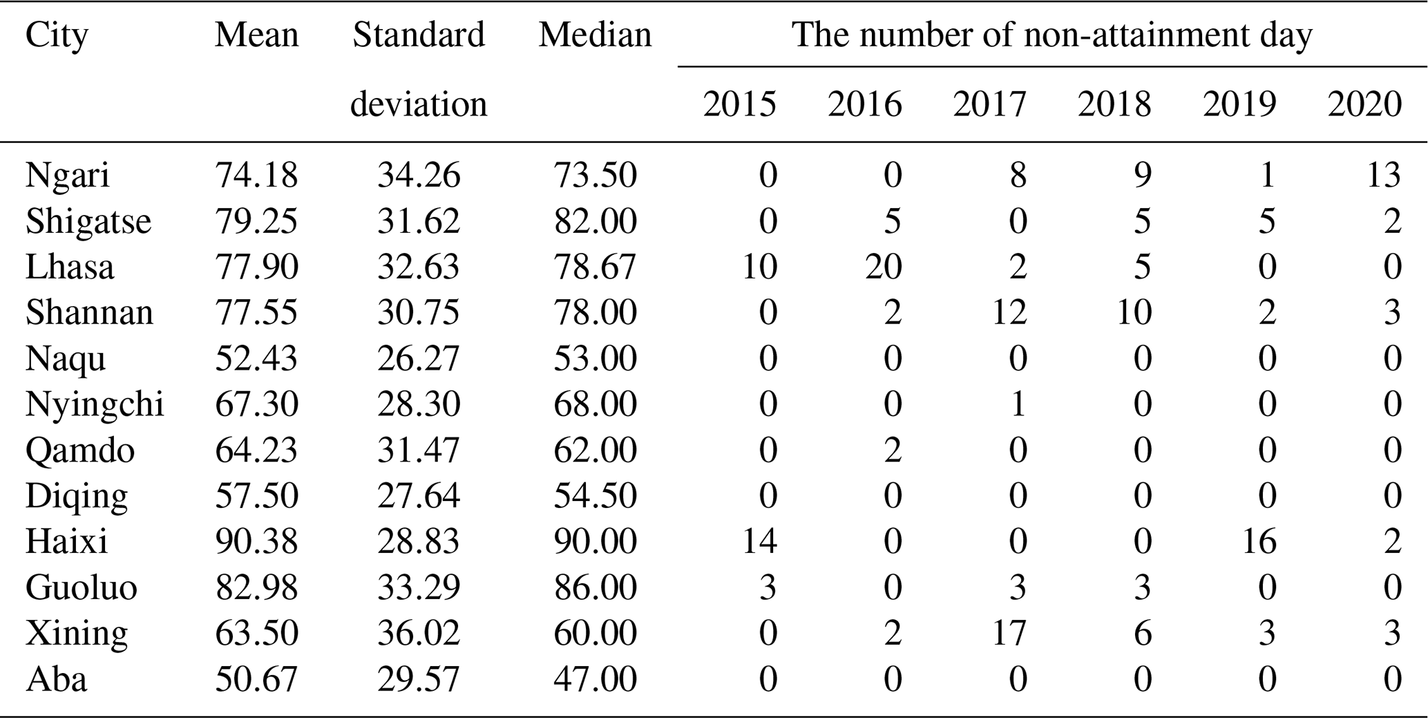
Statistical summary and box plot of surface ozone concentration (units: µg m⁻³) in each city over the QTP from 2015 to 2020 are presented in Table 3 and Fig. S1 in the Supplement respectively. The average of surface ozone between 2015 and 2020 in each city over the QTP varied over 50.67±29.57 to 90.38±28.83 µg m⁻³, and the median value varied over 53.00 to 90.00 µg m⁻³. In comparison, the average surface ozone between 2015 and 2020 in the Beijing-Tianjin-Hebei (BTH), the Fenwei Plain (FWP), the Yangtze River Delta (YRD) and the Pearl River Delta (PRD) in densely populated and highly industrialized eastern China was 140.76, 132.16, 125.09 and 119.82 µg m⁻³ respectively. The average surface ozone between 2011 and  2015 at the suburb Nam Co station in the southern-central part of the QTP was 47.00±12.43 µg m⁻³ (X. Yin et al., 2019). As a result, surface ozone levels in the urban areas over the QTP are much lower than those in urban areas in eastern China but higher than those in the suburban areas over the QTP. Among all cities over the QTP, the highest and lowest surface ozone concentrations occur in Haixi and Aba, with mean values of 90.38±28.83 and 50.67±28.83 µg m⁻³ respectively. Generally, surface ozone concentrations in Qinghai province are higher than those in Tibet province. We also presented the percentile variation of surface ozone concentration (units: µg m⁻³) in each city over the QTP from 2015 to 2020 in Fig. S2. The percentile variation modes of surface ozone concentration in all cities over the QTP are similar. In this study, only mean plus standard variance of surface ozone concentration rather than its percentile variation in each city was investigated. This prevailing method has been used in a number of studies to describe the variabilities of atmospheric compositions over the QTP (Li et al., 2020; Liu et al., 2021; Ma et al., 2020; Xu et al., 2016, 2018; Yin et al., 2017, 2019).

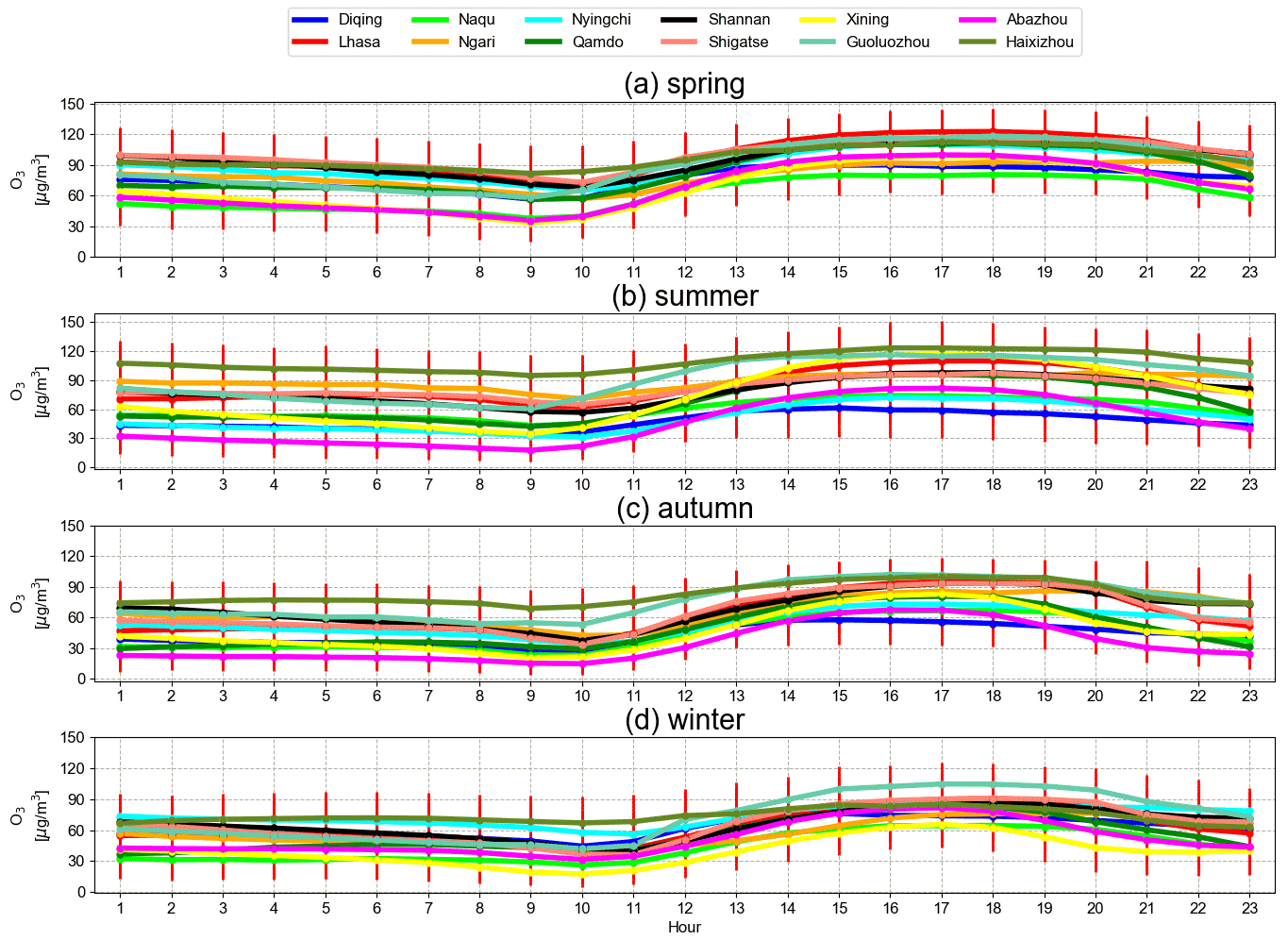
Figure 3 Diurnal cycle of surface ozone (units: µg m⁻³) in each season and each city over the QTP. The vertical error bar is 1σ standard variation (SD) within that hour.

The ambient air quality standard issued by the Chinese government regularized that the critical value (Class 1 limit) for the maximum 8 h average ozone level is 160 µg m⁻³. With this rule, we summarize the number of non-attainment day per year in each city over the QTP in Table 3. The number of non-attainment days per city and per year over the QTP is only 2 between 2015 and 2020. Ozone non-attainment events over the QTP typically occur in spring or summer. In comparison, the number of non-attainment days per city and per year over the BTH, FWP, YRD and PRD is much larger, with values of 78, 36, 82 and 45 between 2015 and 2020 respectively, and all ozone non-attainment events over these regions occur in summer. The number of non-attainment days in Ngari in 2020, Lhasa in 2016 and 2017, Shannan in 2017 and 2018, Haixi in 2015 and 2019, and Xining in 2017 are 13, 10, 20, 12, 10, 14, 16 and 17 d respectively. The number of non-attainment days in all other cities over the QTP are less than 10 d. In particular, surface ozone concentrations in Aba, Naqu and Diqing in all the years between 2015 and 2020 are less than the Class 1 limit of 160 µg m⁻³. There are only 1 and 2 non-attainment days in Nyingchi and Qamdo between 2015 and 2020 respectively.

4.2 Diurnal variability

Diurnal cycles of surface ozone in each season and each city over the QTP are presented in Fig. 3. Overall, diurnal cycle of surface ozone in each city over the QTP presents a unimodal pattern in all seasons. For all cities in all seasons, high levels of surface ozone occur in the daytime (09:00 to 20:00 LT) and low levels of surface ozone occur at nighttime (21:00 to 08:00 LT). As seen from Fig. 3, surface ozone levels usually increase over time starting at 08:00 to 11:00 LT in the morning, reach the maximum values at 15:00 to 18:00 LT in the afternoon, and then decrease over time till the minimum values at 08:00 or 09:00 LT the next day.

The timings of the diurnal cycles in all cities over the QTP were shifted by 1 to 2 h later in winter than those during the rest of the year, most likely due to the later time of sunrise. Yin et al. (2017) also observed such a shift in the diurnal cycle at the suburb Nam Co station. The diurnal cycles of surface ozone in the urban areas over the QTP spanned a large range of −43.73 % to 47.12 % depending on region, season and measurement time. The minimum and maximum surface ozone levels in the urban areas over the QTP varied over (22.89±15.55) to (68.96±18.27) µg m⁻³ and (57.77±21.56) to (102.08±15.14) µg m⁻³ respectively. On average, surface ozone levels in the urban areas over the QTP have mean values of (72.41±33.83) µg m⁻³ during the daytime (08:00–19:00 LT) and (60.89±32.25) µg m⁻³ during the evening (20:00–08:00 LT). The diurnal cycles of surface ozone in all cities over the QTP are generally consistent with the results reported in eastern China and the suburban areas over the QTP (X. Yin et al., 2019; Yin et al., 2017; Zhao et al., 2016; Shen et al., 2014).

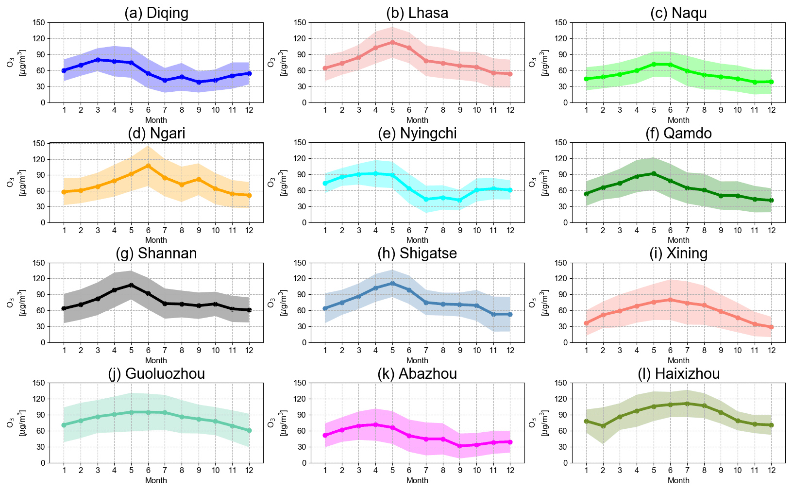
Figure 4 Monthly mean time series of surface ozone (units: µg m⁻³) between 2015 and 2020 in each city over the QTP. The vertical error bar is 1σ standard variation (SD) within that month.

4.3 Seasonal variability

Monthly averaged time series of surface ozone in each city over the QTP between 2015 and 2020 are shown in Fig. 4. Surface ozone levels in all cities over the QTP showed pronounced seasonal features. Seasonal cycles of surface ozone in most cities present a unimodal pattern with a seasonal peak occurring around March-July and a seasonal trough occurring around October–December. Specifically, maximum surface ozone levels occur in spring over Diqing, Lhasa, Naqu, Nyingchi, Qamdo, Shannan, Shigatse and Aba, and occur in summer over Ngari, Xining, Guoluo and Haixi; minimum surface ozone levels in Nyingchi and Diqing occur in autumn, and in other cities they occur in winter. The minimum and maximum surface ozone levels between 2015 and 2020 over the QTP varied over (29.21±19.03) to (60.45±31.35) µg m⁻³ and (71.25±26.53) to (112.46±28.92) µg m⁻³ respectively (Table S1 in the Supplement). The peak-to-trough contrast in Diqing, Naqu, Nyingchi and Aba were smaller than those in other cities. Owing to regional deference in meteorology and anthropogenic emission, the seasonal cycle of surface ozone in the urban areas over the QTP is also regional dependent.

4.4 Inter-annual variability

The inter-annual variability of surface ozone between 2015 and 2020 in each city over the QTP fitted by the bootstrap resampling method is presented in Figs. 5 and S3, and is also summarized in Table S1. Generally, the measured and fitted surface ozone concentrations in each city over the QTP are in good agreement with a correlation coefficient (R) of 0.68–0.92 (Fig. S4). The measured features in terms of seasonality and inter-annual variability can be reproduced by the bootstrap resampling model. However, owing to the year-to-year deference in anthropogenic emission and meteorology, both inter-annual variability and fitting residual were not zero in all cities. The inter-annual trends in surface ozone level from 2015 to 2020 over the QTP spanned a large range of ($-\mathrm{2.43}\pm \mathrm{0.56}$) to (7.55±1.61) µg m⁻³ yr⁻¹, indicating a regional representation of each dataset. The inter-annual trends of surface ozone levels in most cities including Diqing, Naqu, Ngari, Nyingchi, Shannan, Shigatse, Xining, Abzhou and Haixi showed positive trends. The largest increasing trends were presented in Diqing and Nagri, with values of (5.31±1.28) and (7.55±1.61) µg m⁻³ yr⁻¹ respectively. In contrast, surface ozone levels in Lhasa, Qamdo and Guoluo presented negative trends, with values of ($-\mathrm{1.62}\pm \mathrm{0.76}$), ($-\mathrm{2.43}\pm \mathrm{0.56}$) and ($-\mathrm{2.36}\pm \mathrm{0.81}$) µg m⁻³ yr⁻¹ respectively.

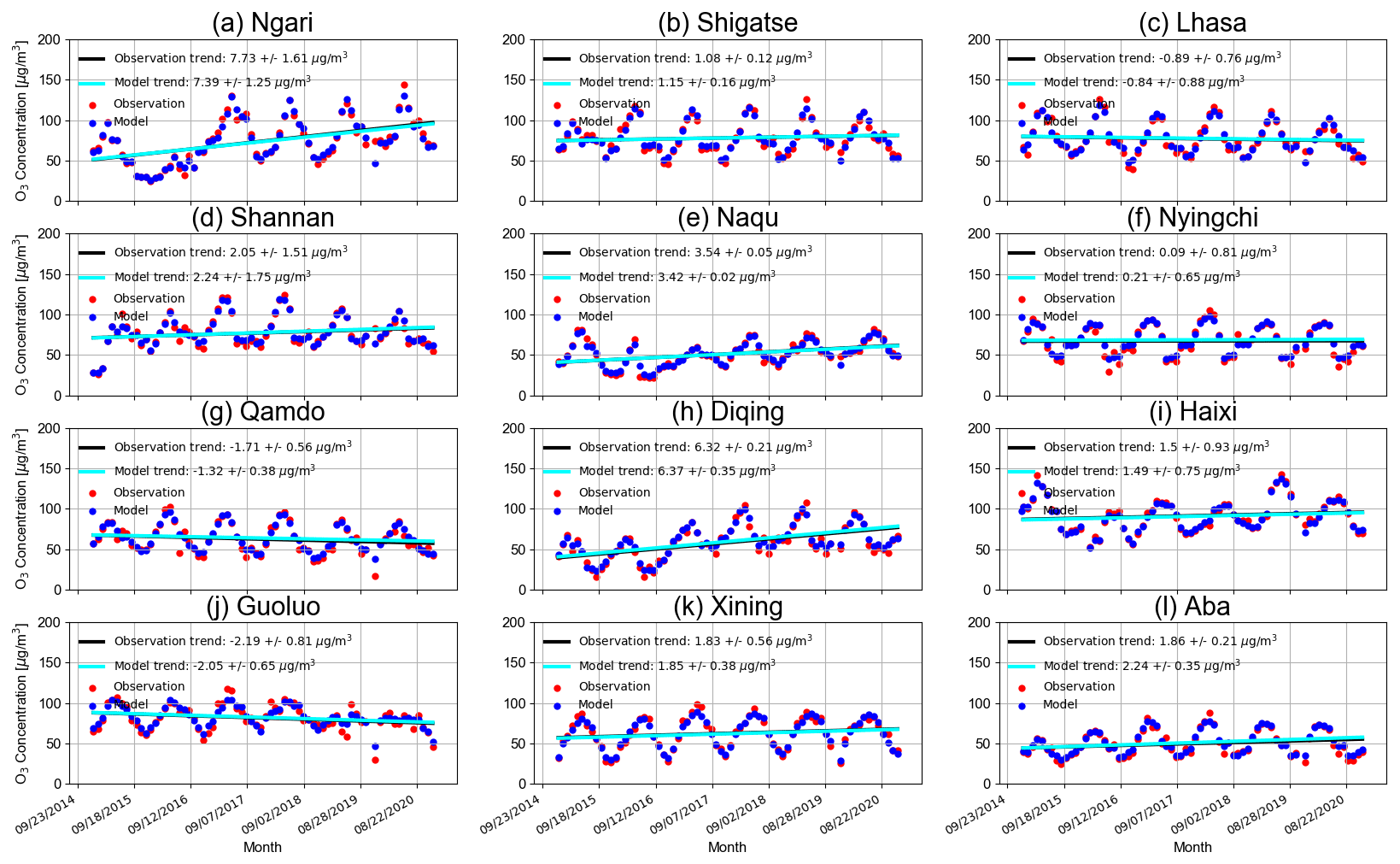
Figure 5 Inter-annual trends of surface ozone levels between 2015 and 2020 in the urban areas over the QTP. Blue dots are the monthly averaged surface ozone measurements. The seasonality and inter-annual variability in each city fitted by using a bootstrap resampling model with a second Fourier series (red dots) plus a linear function (black line) are also shown.

5 Performance evaluation

We evaluate the performance of the RF model in predicting hourly surface ozone level in each city over the QTP using the metrics of Pearson correlation coefficient (R), the root means square error (RMSE), and the mean absolute error (MAE). They are commonly used metrics for evaluation of machine-learning model predictions, and are defined as Eqs. (8)–(10) respectively.

$$\begin{array}{}\text{(8)}& {\displaystyle }& {\displaystyle }R={\displaystyle \frac{n\sum _{i=\mathrm{0}}^n{x}_i{y}_i-\sum _{i=\mathrm{0}}^n{x}_i\cdot \sum _{i=\mathrm{0}}^n{y}_i}{\sqrt{n\sum _{i=\mathrm{0}}^n{x}_i^{\mathrm{2}}-{\left(\sum _{i=\mathrm{0}}^n{x}_i\right)}^{\mathrm{2}}}\cdot \sqrt{n\sum _{i=\mathrm{0}}^n{y}_i^{\mathrm{2}}-{\left(\sum _{i=\mathrm{0}}^n{y}_i\right)}^{\mathrm{2}}}}}\text{(9)}& {\displaystyle }& {\displaystyle }\mathrm{RMSE}=\sqrt{{\displaystyle \frac{\sum _{i=\mathrm{1}}^n{\left(x_i-y_i\right)}^{\mathrm{2}}}{n}}}\text{(10)}& {\displaystyle }& {\displaystyle }\mathrm{MAE}={\displaystyle \frac{\sum _{i=\mathrm{1}}^n\mathrm{|}{x}_i-y_i\mathrm{|}}{n}},\end{array}$$

where x_i and y_i are the ith concurrent measured and predicted data pairs respectively. The n is the number of measurements. The R value represents the fitting correlation between the measurements and predictions. The RMSE value measures the relative average difference between the measurements and predictions. The MAE value measures the absolute average difference between the measurements and predictions. The units of RMSE and MAE are same as the measured data, namely µg m⁻³.

Comparisons between the model predictions and measurements for the testing data (not included in model training) in each city over the QTP are shown in Fig. S5. Overall, the RF model predictions and surface ozone measurements are in good agreement, showing high R and low RMSE and MAE for testing dataset in each city over the QTP (Fig. S5). Depending on cities, the R values varied over 0.85 to 0.94, the RMSE over 10.24 to 17.55 µg m⁻³ and MAE over 7.32 to 12.76 µg m⁻³. The R, RMSE and MAE are independent of city and surface ozone level. The results affirm that our model performs very well in predicting surface ozone levels and variabilities in each city over the QTP.

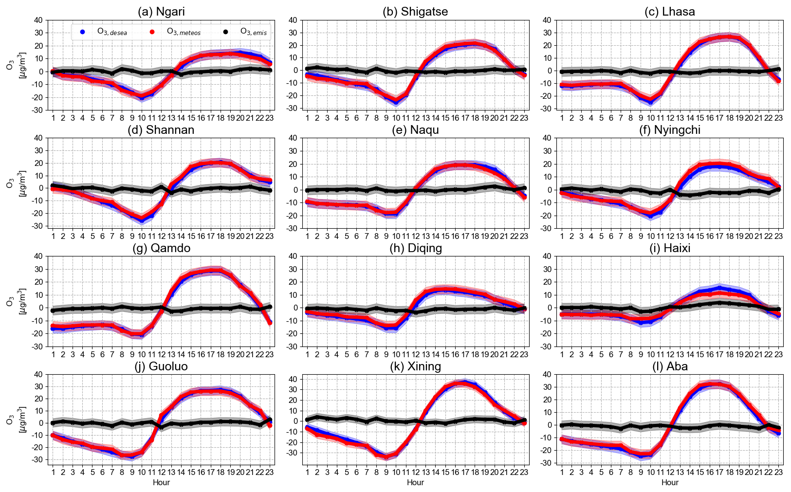
Figure 6 Diurnal cycles of surface ozone anomalies (O_3,anomalies, blue dots and lines) along with the meteorology-driven portions (O_3,meteo, red dots and lines) and the anthropogenic-driven portions (O_3,emis, black dots and lines) in each city over the QTP. Bold curves and the shadows are diurnal cycles and the 1σ standard variations respectively.

We further investigate the importance of each input variable in the RF model for predicting surface ozone level in each city over the QTP. As shown in Fig. S6, time information such as hour term (Hour), year term (Year) or seasonal term (Month) are the most important variables in the RF model predictions in all cities except Xining and Haixi, where temperature term (T_2 m) is the most important variable. For all cities, the aggregate importance of time information is greater than 50 %. In all cities over the QTP, the meteorological variables such as temperature (T_2 m), relative humidity (QV), vertical pressure velocity (OMEGA) and planetary boundary layer height (PBLH) play significant roles when explaining surface ozone concentrations. For other variables, although they are not decisive variables in the RF model predictions, they are not negligible in predicting surface ozone in all cities over the QTP. Although time information is the most important variable in the RF model predictions, it can be used very precisely, and thus the RF model measurement discrepancy in all cities could be from other predictive variables rather than from time information.

6 Drivers of surface ozone anomalies

In this section, we explore the drivers of surface ozone anomalies between 2015 and 2020 over the QTP. We first present descriptively the contributions of anthropogenic emission and meteorology to surface ozone anomalies over the QTP in Sects. 6.1 to 6.3, where statistics on different time scales are summarized. We then present an in-depth analysis of each driver in Sect. 6.4.

6.1 Diurnal scale

Figure 6 presents diurnal cycles of surface ozone anomalies between 2015 and 2020, along with the meteorology-driven and anthropogenic-driven portions in each city over the QTP. In all cities, the anthropogenic contributions are almost constant, but the meteorological contributions show large variations throughout the day. Depending on region and measurement hour, diurnal surface ozone anomalies on average varied over −27.82 to 37.11 µg m⁻³ between 2015 and 2020, whereas meteorological and anthropogenic contributions varied over −33.88 to 35.86 µg m⁻³ and −4.32 to 4.05 µg m⁻³ respectively. The least contrast between meteorological contribution and anthropogenic contribution occurs in Haixi. The diurnal cycles of meteorological contribution are consistent with those of surface ozone anomalies. High levels of meteorological contributions occur during the daytime (09:00 to 20:00 LT) and low levels of meteorological contributions occur in at nighttime. As a result, diurnal surface ozone anomalies in each city over the QTP were mainly driven by meteorology.

Figure 7 Seasonal cycles of surface ozone anomalies (O_3,anomalies, blue dots and lines) along with the meteorology-driven portions (O_3,meteo, red dots and lines) and the anthropogenic-driven portions (O_3,emis, black dots and lines) in each city over the QTP. Bold curves and the shadows are monthly mean values and the 1σ standard variations respectively.

We further investigated the drivers of surface ozone non-attainment events from 2015 to 2020 in each city over the QTP. All ozone non-attainment events were classified as meteorology-dominated or anthropogenic-dominated events according to which one has a larger contribution to the observed surface ozone non-attainment events. The statistical results are listed in Table S2. Except for 1 d in Ngari in 2018, 1 d in Shigatse in 2016 and 1 d in Haixi in 2019, which were dominated by anthropogenic emission, all other surface ozone non-attainment events from 2015 to 2020 over the QTP were dominated by meteorology. Exceptional meteorology drove 97 % of surface ozone non-attainment events from 2015 to 2020 in the urban areas over the QTP. For the meteorology-dominated surface ozone non-attainment events, meteorological and anthropogenic contributions varied over 32.85 to 55.61 µg m⁻³ and 3.67 to 7.23 µg m⁻³ respectively. For the anthropogenic-dominated surface ozone non-attainment events, meteorological and anthropogenic contributions varied over 7.63 to 10.53 µg m⁻³ and 15.63 to 35.28 µg m⁻³ respectively.

6.2 Seasonal scale

Figure 7 presents seasonal cycles of surface ozone anomalies between 2015 and 2020 along with the meteorology-driven and anthropogenic-driven portions in each city over the QTP. In all cities, the monthly averaged surface ozone anomalies between 2015 and 2020 varied with much smaller amplitudes than their diurnal anomalies. Noticeable anomalies include pronounced positive anomalies in December in Nagri, in May in Lhasa, Shannan and Qamdo, in July in Haixi, in June in Guoluo, and negative anomalies in July in Lhasa, Nyingchi and Guoluo. Both meteorological and anthropogenic contributions are regional dependent and show large variations throughout the year. Depending on region and month, meteorological and anthropogenic contributions varied over −4.54 to 3.31 µg m⁻³ and −2.67 to 3.35 µg m⁻³ between 2015 and 2020 respectively.

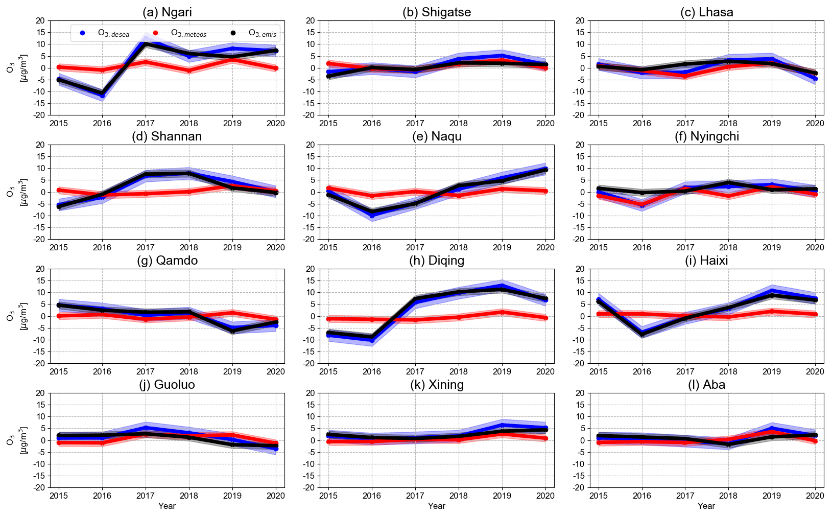
Figure 8 Annual mean surface ozone anomalies (O_3,anomalies, blue dots and lines) along with meteorology-driven portions (O_3,meteo, red dots and lines) and anthropogenic-driven portions (O_3,emis, black dots and lines) in each city over the QTP. Bold curves and the shadows are annual mean values and the 1σ standard variations respectively.

Seasonal surface ozone anomalies between 2015 and 2020 in all cities over the QTP were mainly driven by meteorology. For example, meteorology caused decrements of 3.05 µg m⁻³ in July and 4.27 µg m⁻³ in September in Diqing, whereas anthropogenic emission caused increments of 0.64 and 1.34 µg m⁻³ in respective months. Aggregately, we observed −2.41 and −2.89 µg m⁻³ of seasonal surface ozone anomalies in July and September in Ngari respectively. In all cities, seasonal cycles of meteorological contributions are more consistent with those of surface ozone anomalies over the QTP. In some cases, surface ozone anomalies would have larger values if not for the unfavorable meteorological conditions, e.g., surface ozone anomalies in June in Ngari and in December in Shannan, Guoluo and Aba.

6.3 Multi-year scale

Annual mean surface ozone anomalies between 2015 and 2020, along with meteorology-driven and anthropogenic-driven portions in each city over the QTP are presented in Fig. 8. Surface ozone in Diqing, Naqu, Nagri, Haixi and Shannan shows larger year-to-year variations than that in other cities. Annual mean surface ozone levels in Diqing, Naqu, Nagri and Haixi showed significant reductions of 2.10, 10.32, 6.87 and 15.97 µg m⁻³ respectively, Shannan showed an increment of 9.12 µg m⁻³ and other cities showed comparable values in 2016 relative to 2015. The largest year-to-year difference occurred in Ngari during 2016 to 2017, which has an increment of 25.25 µg m⁻³. The results show that anthropogenic contributions decreased by 1.85, 7.14, 5.65 and 15.98 µg m⁻³ respectively in Diqing, Naqu, Nagri and Haixi, increased by 11.13 µg m⁻³ in Shannan in 2016 relative to 2015 and increased by 20.85 µg m⁻³ in Ngari in 2017 relative to 2016. As a result, all above reductions or increments in surface ozone level were mainly driven by anthropogenic emission. In contrast, surface ozone anomalies in Lhasa in 2017 and 2020, and in Shigatse and Nyingchi in 2019, were mainly driven by meteorology.

Table S3 summarizes the inter-annual trends of surface ozone anomalies, meteorological and anthropogenic contributions from 2015 to 2020 in each city over the QTP. Except for Guoluo, Qamdo and Lhasa, which show decreasing trends, anthropogenic contributions in all other cities showed increasing trends from 2015 to 2020. With respect to meteorology contribution, Ngari, Naqu, Diqing and Haixi showed increasing trends from 2015 to 2020 and all other cities showed decreasing trends. The inter-annual trends of surface ozone anomalies in Ngari, Lhasa, Naqu, Qamdo, Diqing, Haixi and Guoluo can be attributed to anthropogenic emissions in 95.77 %, 96.30 %, 97.83 %, 82.30 %, 99.26 % and 87.85 %, and to meteorology in 4.23 %, 3.70 %, 2.17 %, 3.19 %, 0.74 % and 12.15 % respectively. The inter-annual trends of surface ozone in other cities were fully driven by anthropogenic emission, where the increasing inter-annual trends would have larger values if not for the favorable meteorological conditions. As a result, the inter-annual trends of surface ozone anomalies in all cities over the QTP were dominated by anthropogenic emission.

6.4 Discussions

Typically, all cities over the QTP are formed in flat valleys, with surrounding mountains rising to more than 5.0 km a.s.l., and maintain continuous expansion and development over time. Inhibited by surrounding mountains, regional-dependent emissions and mountain peak-valley meteorological systems result in regional representation of surface ozone level and their drivers on diurnal, seasonal and inter-annual scales.

Correlations between O_3,meteo and each meteorological anomaly are summarized for all time, for the diurnal scale, for the seasonal scale and for the multi-year scale in Tables S4–S7. We find that all-time scales of meteorology-driven surface ozone anomalies in each city are positively related to anomalies of temperature, planetary boundary layer height (PBLH), surface incoming shortwave flux (SWGDN), downward transport velocity at the PBLH (OMEGA), and tropopause height (TROPH). Among all these positive correlations, the correlations with temperature, PBLH and SWGDN in all cities are higher than those with OMEGA and TROPH. As high temperature and SWGDN facilitate the formation of ozone via the increase in chemical reaction rates or biogenic emissions, the meteorology-driven surface ozone anomalies have the highest correlations with the changes in temperature and SWGDN. Possible reasons for the ozone increases with the increase in PBLH include lower NO concentration at the urban surface owing to the deep vertical mixing, which then limits ozone destruction and increases ozone concentrations (He et al., 2017), and more downward transport of ozone from the free troposphere, where the ozone concentration is higher than the near-surface concentration (Sun et al., 2009). Large OMEGA and high tropopause height also facilitate downward transport of stratospheric ozone, resulting in a high surface ozone level. The QTP has been identified as a hot spot for stratospheric–tropospheric exchange (Cristofanelli et al., 2010; Škerlak et al., 2014), where the surface ozone is elevated from the baseline during the spring owing to frequent stratospheric intrusions. Generally, surface ozone anomalies are negatively related to humidity, rainfall and total cloud fraction in each city over the QTP. These wet meteorological conditions inhibit biogenic emissions, slow down ozone chemical production, and facilitate the ventilation of ozone and its precursors (Gong and Liao, 2019; Jiang et al., 2021; Lu et al., 2019a, b; Ma et al., 2019), and therefore contribute to ozone decrease.

The U_10 m and V_10 m represent the metrics for evaluating the horizontal transport. In most of the cities over the QTP, noticeable ozone versus horizontal wind correlations are observed, indicating that horizontal transport is an important contributor to surface ozone (Shen et al., 2014; Zhu et al., 2004). The QTP region, as a whole, is primarily regulated by the interplay of the Indian summer monsoon and the westerlies, and the atmospheric environment over the QTP is heterogeneous. Mount Everest is representative of the Himalayas on the southern edge of the Tibetan Plateau and is close to South Asia, where anthropogenic atmospheric pollution has been increasingly recognized as disturbing the high mountain regions (Decesari et al., 2010; Maione et al., 2011; Putero et al., 2014). The northern QTP, including Xining, Haixi and Guoluo, is occasionally influenced by regional polluted air masses (Xue et al., 2011; Zhu et al., 2004), in particular, the impacts of anthropogenic emissions from central and eastern China in the summer (Xue et al., 2011). The cities over the inland QTP are distant from both South Asia and northwestern China; this area has been found to be influenced by episodic long-range transport of air pollution from South Asia (Lüthi et al., 2015), evidenced by the study of aerosol and precipitation chemistry in these cities (Cong et al., 2010).

In order to determine which specific meteorological variables are responsible for the meteorology-dominated ozone non-attainment events over the QTP, we have investigated the correlations between each meteorological variable and ozone anomalies in each city during the ozone non-attainment days. As tabulated in Table S8, temperature is the dominant meteorological variable responsible for the meteorology-dominated ozone non-attainment events, especially in Shigatse, Lhasa, Shannan, Haixi and Guoluo. In addition, the OMEGA is an important meteorological variable in most cities, especially in Guoluo, where the correlation is up to 0.69. For other meteorological variables, winds (U_10 m, V_10 m) and TROPH also have noticeable contributions to some ozone non-attainment events.

The NO_x and VOCs are the main precursors of surface ozone. The monthly and annual averaged anthropogenic emissions of NO_x and VOCs in each city over the QTP extracted from the Multi-resolution Emission Inventory for China (MEIC) between 2015 and 2017 are presented in Tables S9–S12. Major anthropogenic emissions in each city over the QTP are from the transport sector and residential sector, including burning emissions of coal, post-harvest crop residue, yak dung and religious incense (Chen et al., 2009; Kang et al., 2016, 2019; Li et al., 2017). The NO_x and VOCs emissions have decreased in Diqing, Naqu, Nagri in 2016 relative to 2015. These reductions of NO_x and VOCs emissions have jointly driven the changes of ozone in these cities. Although NO_x emissions increased in Haixi during 2015 to 2016, VOCs emissions have significantly decreased by 6.82 t. As a result, the decreases in ozone in Haixi in 2016 relative to 2015 were attributed to VOCs reductions during the same period.

The correlations of the monthly and annual averaged anthropogenic contributions against the NO_x and VOCs emissions are summarized in Table S13. The correlations of the monthly averaged anthropogenic contributions against anthropogenic NO_x and VOCs emissions are within the range 0.35–0.81 and 0.33–0.83 respectively. For the annual averaged statistics, the correlations against NO_x and VOCs emissions are within the range 0.15–0.94 (except for Nyingchi and Diqing), and 0.34–0.98 (except for Haixi) respectively. For all cities except for Shannan, Qamdo and Haixi, both the NO_x and VOCs emissions are consistent with the anthropogenic contributions. although only NO_x emissions in Qamdo and Haixi and VOCs emissions in Shannan are consistent with anthropogenic contributions. In general, the changes in NO_x and VOCs emissions in the MEIC are able to explain the variabilities of both monthly and annual averaged anthropogenic contributions.

7 Conclusions

In this study, we have investigated the evolutions, implications and the drivers of surface ozone anomalies (defined as deviations of ozone levels relative to their seasonal means) between 2015 and 2020 in the urban areas over the QTP. Diurnal, seasonal and inter annual variabilities of surface ozone in 12 cities over the QTP are analyzed. The average surface ozone between 2015 and 2020 in each city over the QTP varied over (50.67±29.57) to (90.38±28.83) µg m⁻³, and the median value varied over 53.00 to 90.00 µg m⁻³. Overall, the diurnal cycle of surface ozone in each city over the QTP presents a unimodal pattern in all seasons. For all cities in all seasons, high levels of surface ozone occur in the daytime (09:00 to 20:00 LT) and low levels of surface ozone occur at nighttime (21:00 to 08:00 LT). Seasonal cycles of surface ozone in most cities present a unimodal pattern with a seasonal peak occurring around March–July and a seasonal trough occurring around October–December. The inter-annual trends in surface ozone level from 2015 to 2020 over the QTP spanned a large range of ($-\mathrm{2.43}\pm \mathrm{0.56}$) to (7.55±1.61) µg m⁻³ yr⁻¹, indicating a regional representation of each dataset.

We have established a RF regression model to describe the relationships between hourly surface ozone concentrations (response variables) and their potential driving factors (predictive variables) in the urban areas over the QTP. The RF model predictions and surface ozone measurements are in good agreement, showing high R and low RMSE and MAE in each city over the QTP. Depending on the city, the R values varied over 0.85 to 0.94, the RMSE over 10.24 to 17.55 µg m⁻³ and the MAE over 7.32 to 12.76 µg m⁻³. The R, RMSE and MAE are independent of city and surface ozone levels. The results affirm that our model performs very well in predicting surface ozone levels and variabilities in each city over the QTP.

We have separated quantitatively the contributions of anthropogenic emission and meteorology to surface ozone anomalies by using the RF model-based meteorological normalization method. Diurnal and seasonal surface ozone anomalies over the QTP were mainly driven by meteorology, and inter-annual anomalies were mainly driven by anthropogenic emission. Depending on the region and the measurement hour, diurnal surface ozone anomalies varied over −30.55 to 34.01 µg m⁻³ between 2015 and 2020, whereas meteorological and anthropogenic contributions varied over −20.08 to 48.73 µg m⁻³ and −27.18 to 1.92 µg m⁻³ respectively. Unfavorable meteorology drove 97 % of surface ozone non-attainment events between 2015 and 2020 in the urban areas over the QTP. Monthly averaged surface ozone anomalies varied with much smaller amplitudes than their diurnal anomalies, whereas meteorological and anthropogenic contributions varied over 7.63 to 55.61 µg m⁻³ and 3.67 to 35.28 µg m⁻³ between 2015 and 2020 respectively. The inter-annual trends of surface ozone anomalies in Ngari, Lhasa, Naqu, Qamdo, Diqing, Haixi and Guoluo can be attributed to anthropogenic emissions in 95.77 %, 96.30 %, 97.83 %, 82.30 %, 99.26 % and 87.85 %, and to meteorology in 4.23 %, 3.70 %, 2.17 %, 3.19 %, 0.74 % and 12.15 % respectively. The inter-annual trends of surface ozone anomalies in other cities were fully driven by anthropogenic emission, where the increasing inter-annual trends would have larger values if not for the favorable meteorological conditions. This study can not only improve our knowledge with respect to spatiotemporal variability of surface ozone but also provide valuable implications for ozone mitigation over the QTP.