Inverse modelling of Chinese NO_x emissions using deep learning: integrating in situ observations with a satellite-based chemical reanalysis

Nitrogen dioxide (NO₂) column density measurements from satellites have been widely used in constraining emissions of nitrogen oxides (NO_x = NO + NO₂). However, the utility of these measurements is impacted by reduced observational coverage due to cloud cover and their reduced sensitivity toward the surface. Combining the information from satellites with surface observations of NO₂ will provide greater constraints on emission estimates of NO_x. We have developed a deep-learning (DL) model to integrate satellite data and in situ observations of surface NO₂ to estimate NO_x emissions in China. A priori information for the DL model was obtained from satellite-derived emissions from the Tropospheric Chemistry Reanalysis (TCR-2). A two-stage training strategy was used to integrate in situ measurements from the China Ministry of Ecology and Environment (MEE) observation network with the TCR-2 data. The DL model is trained from 2005 to 2018 and evaluated for 2019 and 2020. The DL model estimated a source of 19.4 Tg NO for total Chinese NO_x emissions in 2019, which is consistent with the TCR-2 estimate of 18.5 ± 3.9 Tg NO and the 20.9 Tg NO suggested by the Multi-resolution Emission Inventory for China (MEIC). Combining the MEE data with TCR-2, the DL model suggested higher NO_x emissions in some of the less-densely populated provinces, such as Shaanxi and Sichuan, where the MEE data indicated higher surface NO₂ concentrations than TCR-2. The DL model also suggested a faster recovery of NO_x emissions than TCR-2 after the Chinese New Year (CNY) holiday in 2019, with a recovery time scale that is consistent with Baidu “Qianxi” mobility data. In 2020, the DL-based analysis estimated about a 30 % reduction in NO_x emissions in eastern China during the COVID-19 lockdown period, relative to pre-lockdown levels. In particular, the maximum emission reductions were 42 % and 30 % for the Jing-Jin-Ji (JJJ) and the Yangtze River Delta (YRD) mega-regions, respectively. Our results illustrate the potential utility of the DL model as a complementary tool for conventional data-assimilation approaches for air quality applications.

1 Introduction

Nitrogen oxides (NO_x = NO + NO₂) are a family of primary air pollutants that are directly involved in the formation of other air pollutants, such as tropospheric ozone and secondary inorganic aerosols. Emitted by anthropogenic and natural sources on the surface, NO_x also has sources from lightning in the free troposphere (Murray, 2016). Satellite observations of tropospheric NO₂ columns have been widely used during the past 2 decades to constrain NO_x emissions (referred to as “top-down” emissions). Martin et al. (2003) used a mass balance approach with the GEOS-Chem global chemical transport model (CTM) to relate changes in the NO₂ column to NO_x emissions at the surface. They showed that the top-down analysis could reduce regional uncertainties in the a priori NO_x emissions. Satellite-derived NO_x emissions have been obtained by several subsequent studies using a similar mass balance approach (Bertram et al., 2005; Konovalov et al., 2006; Kim et al., 2006; Martin et al., 2006; Toenges-Schuller et al., 2006; Boersma et al., 2008). Advanced data-assimilation methods have also been applied to obtain satellite-based emission estimates of NO_x. For example, the four-dimensional variational (4D-Var) method uses a CTM and its adjoint to propagate the differences between satellite data and simulation to the a priori estimate of NO_x emissions (Müller and Stavrakou, 2005; Kurokawa et al., 2009; Chai et al., 2009; Qu et al., 2019). The Kalman filter is another widely used method, which employs information about the error covariance in the forecast of the trace gases to update atmospheric quantities in the CTMs (Napelenok et al., 2008; Miyazaki et al., 2020a; Wu et al., 2020).

Despite the range of inverse modelling approaches used to estimate NO_x emissions from satellite observations, they all suffer from potential limitations associated with the CTMs employed in the inversion analyses. For example, Lin and McElroy (2010) found that a different scheme for mixing in the planetary boundary layer could lead to 3 %–14 % differences in the top-down NO_x emission budgets for East China. Deep convective transport in the free troposphere, which can be challenging to accurately simulate, could vertically transport NO₂ generated by lightning activities, which results in greater nonlinearity between NO_x emissions and NO₂ columns (Choi et al., 2005; Nault et al., 2017). The lifetime of NO_x varies diurnally and seasonally, and discrepancies in the ability of a CTM to capture these variations will contribute to uncertainties in the top-down NO_x emission estimates (Beirle et al., 2011; de Foy et al., 2014; Liu et al., 2016).

An additional limitation with the satellite-based top-down emission estimates of NO_x is that NO₂ is highly concentrated near the surface, whereas satellite measurements have lower sensitivity near the surface (Boersma et al., 2016). As a result, it is challenging for satellite observations to capture changes in surface NO_x emissions. It has been suggested that satellite NO₂ measurements are blending information from both surface emissions and atmospheric background of NO₂ due to the low sensitivity of the satellite retrievals to NO₂ near the surface (Li and Wang, 2019; Silvern et al., 2019; Qu et al., 2021). In situ observations of surface NO₂ are more representative of local emissions, but typically have more limited observational coverage. As a result, combining the surface observations with the satellite data could offer greater constraints on NO_x emission estimates.

Here we use a deep-learning (DL) model to indirectly integrate satellite data and in situ observations of surface NO₂ to estimate NO_x emissions in China. Deep-learning and other machine-learning models have been increasingly used in the field of atmospheric science (Rasp et al., 2018; He et al., 2022; Keller and Evans, 2019). These data-driven methods show high skill in capturing the nonlinear relationship between correlated atmospheric quantities. Compared to conventional data-assimilation systems, DL models are free of errors in chemistry and the potential errors associated with defective parameterization of subgrid-scale processes (Rasp et al., 2018). Moreover, high-resolution data assimilation using conventional approaches is computationally expensive, especially when dealing with large amounts of data, whereas DL models show much higher computational efficiency for high-resolution data-rich applications. In the present work, we use a DL model to estimate Chinese NO_x emissions using surface NO₂ concentrations. We train the DL model twice with different input information used in each training stage. We use the two-stage transfer learning strategy to integrate in situ NO₂ observations from the China Ministry of Ecology and Environment (MEE) network with the Tropospheric Chemical Reanalysis (TCR-2) that assimilated satellite observations.

We focus on the 2019–2020 period, which overlaps with the COVID-19 pandemic that led to the lockdown of over one-third of Chinese cities in early 2020. Observations have shown significant reductions of atmospheric abundances of NO₂ over China during this period (Bauwens et al., 2020; Liu et al., 2020). The change in atmospheric NO₂ implies an anomalous change in emission of NO_x, which provides a unique opportunity to evaluate the utility of the DL model for estimating NO_x emissions. We evaluate the performance of the DL model by analysing the predicted NO_x emissions for the normal year 2019 and the anomalous year 2020. Evaluation of the DL-based system utilized the dependent testing data set from the TCR-2 standard product (based on data from the Ozone Monitoring Instrument (OMI)), an updated higher-resolution TCR-2 product constrained by the TROPOspheric Monitoring Instrument (TROPOMI) measurements, and the independent Baidu “Qianxi” mobile data (Kraemer et al., 2020; Zhang et al., 2021).

The outline of the paper is as follows. Section 2 describes the data sets used in the analysis, the DL model, and the two-stage training strategy. Section 3 shows the results from the evaluation of the model performance after the two training stages and the analyses of the Chinese NO_x emissions for 2019 and 2020. Conclusions are presented in Sect. 4.

2 Data and methods

2.1 TCR-2 data products

The TCR-2 chemical data set (Miyazaki et al., 2020a) was generated using a local ensemble transform Kalman filter (LETKF) data-assimilation system (Hunt et al., 2007), which optimizes both emissions and atmospheric abundance of various chemical species from the assimilation of multi-constituent measurements from multiple satellite instruments. The observational data are assimilated into the MIROC-CHASER global CTM (Sudo et al., 2002; Sekiya et al., 2018). The TCR-2 data product has a horizontal resolution of $\mathrm{1.1}{}^{\circ }\times \mathrm{1.1}{}^{\circ }$, and consists of 27 pressure levels from 1000 to 60 hPa. Details about the TCR-2 data-assimilation system can be found in Miyazaki et al. (2020a).

The TCR-2 NO_x emissions were constrained in part by tropospheric NO₂ column retrievals from the QA4ECV version 1.1 level 2 product for Ozone Monitoring Instrument (OMI) NO₂ measurements (Boersma et al., 2018). The OMI is a spectrometer on board the NASA Aura spacecraft that was launched on 15 July 2004. It measures NO₂ in the UV-VIS range of the spectrum, from which vertical column densities (VCD) of NO₂ are retrieved. The OMI measurement strategy provides global coverage once per day. It should be noted that as a chemical data-assimilation system with detailed tropospheric chemistry, TCR-2 also relies on observational constraints from other NO₂-related chemical species (e.g. tropospheric ozone) to optimize tropospheric NO₂ and NO_x emissions. For the analysis conducted here, the TCR-2 surface NO₂ concentrations and NO_x emissions were averaged to daily fields to train the DL model. In addition to the standard TCR-2 product, we also used an updated version of the TCR-2 products that assimilated tropospheric NO₂ column retrievals from the TM5-MP-DOMINO data product version 1.2 for TROPOMI (van Geffen et al., 2020) at a higher spatial resolution of 0.5625^∘ (referred to as the T213 product Miyazaki et al., 2020b, 2021). TROPOMI serves as the continuation and the next generation of the OMI sensor, monitoring air pollutants at a much higher horizontal resolution (7 km × 3.5 km at nadir), and data have been available since February 2018. Since the TROPOMI-based TCR-2 T213 product is only available for the last few years of the analysis period considered here, we use it as an independent data set in the evaluation of the DL model for the year 2020.

2.2 MEE network

As part of the Chinese government's Air Pollution Control Action Plan, the Ministry of Ecology and Environment (MEE) of the People’s Republic of China (PRC) have been deploying ground-based stations to monitor air pollution since 2013. Surface NO₂ concentration measurements are archived at an hourly frequency, at more than 1500 ground-based stations as of 2019. The NO₂ concentrations are measured and reported in micrograms per cubic metre (µg m⁻³). Special attention is given to the reference state for unit conversion. Until 31 August 2018, the reference state for in situ measurements was 273 K and 1013 hPa, after which it was changed to 298 K and 1013 hPa. To simplify the integration of the MEE data with the TCR-2 data, the in situ measurements were aggregated to the $\mathrm{1.1}{}^{\circ }\times \mathrm{1.1}{}^{\circ }$ grid of the TCR-2 system using the nearest neighbour interpolation method. The locations of the MEE sites as of 2019 are shown in Fig. 1. The MEE network has good coverage over eastern and central China. For western and northeastern China, the spatial coverage is lower. Han et al. (2022) investigated the impact of observational coverage by removing 10 % of the grid-averaged observations from the training of a similar DL model and found no noticeable performance degradation in the evaluation of the DL model over these regions. However, the low station densities in some grids could lead to representation errors in the aggregated observations. The MEE network includes both urban and rural sites and we included data from all sites to increase observational coverage and mitigate representation errors. The MEE measurements are made using a chemiluminescence analyser with a molybdenum converter that results in an overestimation of NO₂ (Lamsal et al., 2008). Following Lamsal et al. (2008), we used the GEOS-Chem model to simulate NO_x, HNO₃, peroxyacetyl nitrate (PAN), and alkyl nitrates (AN) to produce correction factors (CFs) for the measurements using the following relationship:

$$\begin{array}{}\text{(1)}& \mathrm{CF}={\displaystyle \frac{\left[{\mathrm{NO}}_{\mathrm{2}}\right]}{\left[{\mathrm{NO}}_{\mathrm{2}}\right]+\mathrm{0.95}\left[\mathrm{PAN}\right]+\mathrm{0.35}\left[{\mathrm{HNO}}_{\mathrm{3}}\right]+\sum \left[\mathrm{AN}\right]}},\end{array}$$

where ∑AN is the sum of all ANs. We used version 12.0.2 of GEOS-Chem at a resolution of $\mathrm{2}{}^{\circ }\times \mathrm{2.5}{}^{\circ }$ to estimate monthly mean CFs for 2015. The simulation was conducted with full chemistry and the MIX inventory (Li et al., 2017). The annual total Chinese emissions in the simulation was 19.0 Tg NO, which is consistent with TCR-2 estimates. These 2015 CFs were regridded to the $\mathrm{1.1}{}^{\circ }\times \mathrm{1.1}{}^{\circ }$ resolution of the DL model and applied to the MEE measurements for 2014–2020. The CFs were close to unity in high emission regions, such as in eastern China, but could be as small as 0.4 in rural regions.

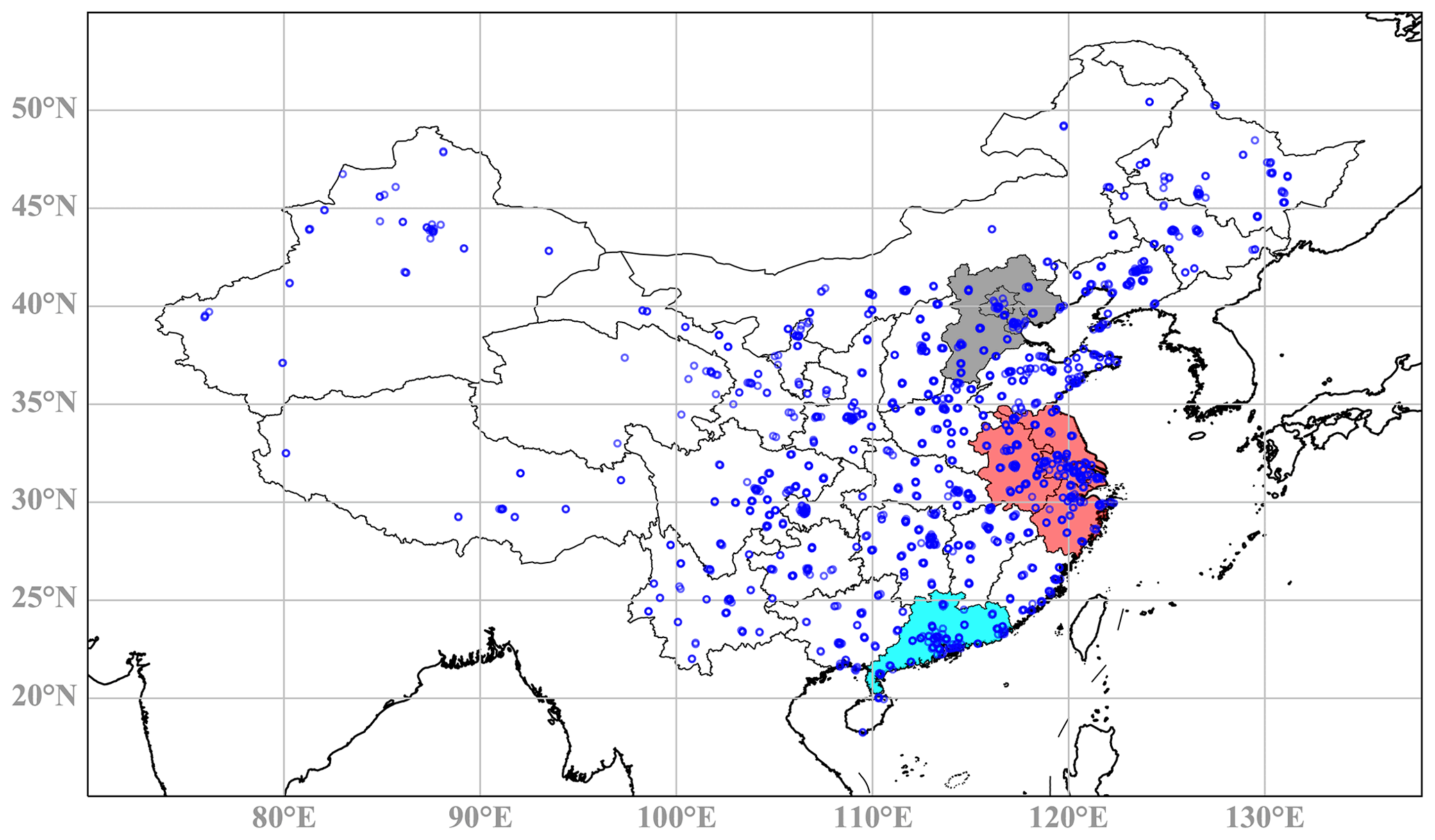
Figure 1 Location of the MEE network stations as of 2019. Blue circles represent the MEE stations. The three metropolitan regions that we focused on in the analysis are shaded in grey, red, and cyan, for Jing-Jin-Ji (JJJ), the Yangtze River Delta (YRD), and the Pearl River Delta (PRD), respectively.

2.3 Baidu “Qianxi” mobile data

The Baidu “Qianxi” mobile data are generated from the Baidu map service, which is widely used in China as an equivalent to Google maps. It quantifies the intensity of human mobility as an immigration index (I-index), an emigration index (E-index), and an intra-city index (C-index). These migration indices have been used by other studies and are shown to have good correlation with human activities (Wei and Wang, 2020; Kraemer et al., 2020; Zhang et al., 2021). The C-index measures the movement of people out of their homes in the city, reflecting intra-city movement, and is thus a proxy of human activity. Zhang et al. (2021) found that the C-index showed much higher correlation with variations in surface NO₂ concentration than the other two indices (the I-index and the E-index). They found that about 40 % of the variance of emission-based NO₂ reductions in 29 megacities (with populations over 8 million) in China could be explained by the C-index. For some megacities in southern China, the variance explained by the C-index was as large as 70 %. The Zhang et al. (2021) results suggest that human mobility can provide a proxy for NO_x emissions. We therefore use the C-index here as the independent data set to evaluate the DL model.

2.4 Deep-learning (DL) model and input variables

The DL model used here is built using convolutional neural networks (CNNs) (LeCun et al., 2015) and long short-term memory (LSTM) units (Hochreiter and Schmidhuber, 1997). Figure 2 shows a schematic diagram of the model. The hybrid architecture was previously used for predicting summertime surface ozone concentrations in the United States in He et al. (2022). The DL model showed great predictive skill in capturing the nonlinear relationship between the predictors and the model output. This DL architecture is applied here for estimating Chinese NO_x emissions using surface NO₂ concentrations and meteorological variables as input predictors. The input variables are forwarded to three sequential convolutional blocks. Each convolutional block consists of two CNN layers and one max-pooling layer. Each CNN layer uses filters that are 3×3 in size to apply convolutional operations with the data vectors and output so-called latent vectors. The softplus function is applied to activate the output from each CNN layer to increase the nonlinearity of the DL architecture. The max-pooling layers further condense the dimension of the latent vectors by taking the maximum values within 2×2 windows. The first three convolutional blocks were used as an encoder for the extraction of spatial features hidden in the input information. The output of the last convolutional block was a highly compressed and reshaped latent vector with a size of 30×1024, which was then forwarded to two LSTM cells, which are recurrent neural networks (RNNs), with 1024 units to learn the dynamics. The LSTM cell is followed by three up-convolutional layers and seven convolutional layers. The up-convolutional layers use 2×2 convolutional filters to up-sample the latent vectors to high-resolution outputs. We applied residual learning connections (the arrows in Fig. 2), which stabilize the performance of the U-net model (Li et al., 2018; He et al., 2016). We used the Adam optimizer for boosted optimization of the U-net model (Kingma and Ba, 2014). The DL model was run on the NVIDIA T4 tensor core graphics processing unit (GPU) on the Graham supercomputer of Compute Canada. During the training process, the convolutional filters, the weight matrices, and bias vectors in the LSTM were iteratively optimized using a back-propagation algorithm. The initial learning rate was $\mathrm{1}\times {\mathrm{10}}^{-\mathrm{5}}$ for both training stages, and the residual sum of squares was used as the loss function. Other hyper-parameters for the training of the model include the number of epochs, which was 250, and the batch size, which was 30.

The meteorological variables were taken from the ERA5 data product, which is different from the ERA-Interim data product used in the TCR-2 data-assimilation system. We chose the more recent ERA-5 product because of its higher spatial and temporal resolution, which better represents mesoscale to synoptic-scale transport processes (Hoffmann et al., 2019). This could be advantageous for the Stage 2 training, where the MEE in situ observations are used to improve the NO₂–NO_x relationship. Table 1 lists the chosen input variables for the U-net model. We treated information of surface NO₂ from days t and t−1 as different channels in the input layer. Considering the short lifetime of surface NO_x, we did not include meteorological variables from day t−1. We included surface NO₂ from days t and t−1 for better prediction of NO_x emissions. All the input variables are regridded to the $\mathrm{1.1}{}^{\circ }\times \mathrm{1.1}{}^{\circ }$ grid of TCR-2 using the first-order conservative remapping algorithm. As mentioned above, the output of the DL model, which is NO_x emissions, is at the same $\mathrm{1.1}{}^{\circ }\times \mathrm{1.1}{}^{\circ }$ grid. To ensure stability of the training of the DL model, all the input variables were scaled to make sure the values are within a relatively similar range. Table 1 gives the details about the input variables selected for the NO_x emission inversions.

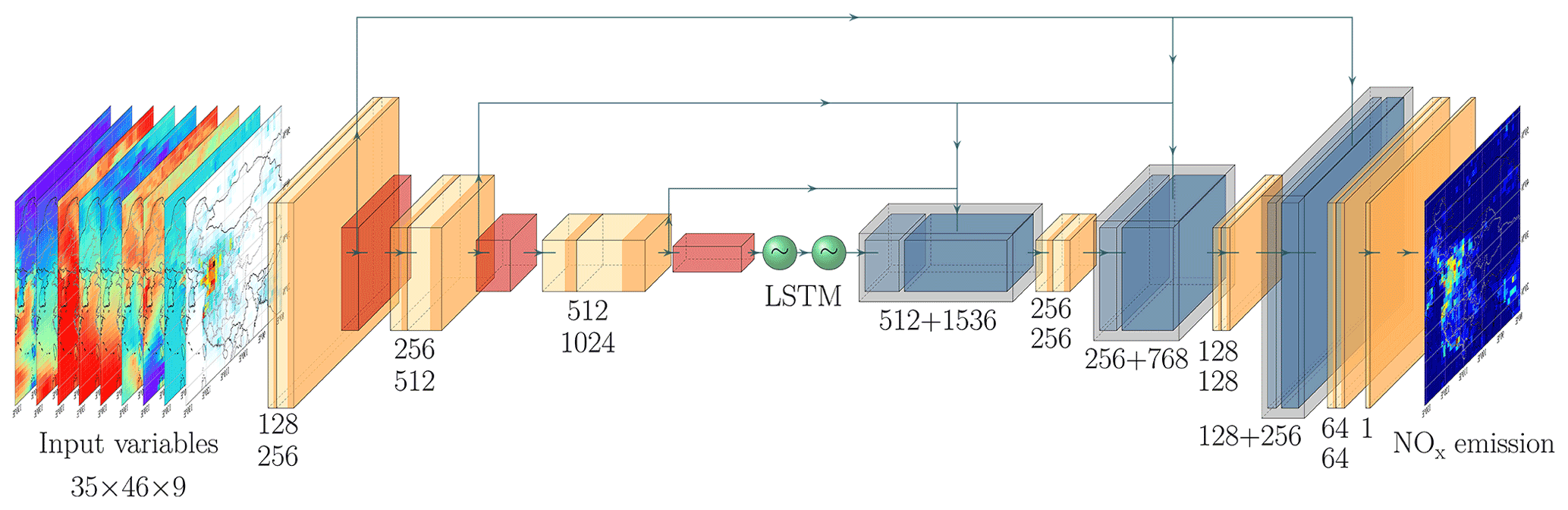
Figure 2 Schematic representation of the U-net model for the prediction of Chinese NO_x emissions. The CNN layers with 3×3 filters are shown in orange. The dark orange regions indicate the application of softplus activation functions. The 2×2 max-pooling layers are shown in red. The two green circles represent the LSTM cells. The 2×2 up-convolutional layers are shown in light blue, which are concatenated (indicated as grey boxes) with the transferred latent vectors (shown as dark blue boxes) from the encoder. The arrows indicate the residual connections.

Table 1 Input variables for NO_x emission inversion using the DL model.

¹ Units of the raw data could be different from these units. Multiplicative scaling is done to match these units before being used by the U-net model. ² TCR-2 surface NO₂ concentrations are used for the first training stage. The MEE in situ NO₂ measurements are added in the second training stage.

2.5 Two-stage training strategy

For the integration of the MEE in situ data with the TCR-2 data, we use a two-stage transfer learning strategy (Zhuang et al., 2021), as depicted in Fig. 3. The first training stage focuses on the TCR-2 NO₂ concentration and NO_x emission relationship. In this training stage, we train the model using the TCR-2 data pairs of NO₂ and NO_x, together with the ERA5 meteorological predictors. The purpose of this training stage is to supervise the DL model with the prior knowledge of the relationship between surface NO₂ concentrations and NO_x emissions from the TCR-2 system. The goal here is to train the DL model to reproduce the TCR-2 NO_x emissions, given the TCR-2 surface NO₂ data. The second training stage is conducted based on the pre-trained DL model from Stage 1. This stage utilizes the transferred TCR-2 knowledge and the pre-trained DL model weights to provide an initial model state for Stage 2. In this second stage, the MEE NO₂ data are integrated with the TCR-2 surface NO₂ data and the model retrained with the combined data set. The purpose of Stage 2 is to improve the relationship between surface NO₂ and NO_x emissions acquired from TCR-2, given the available surface NO₂ observations. Figure 4 shows the annual mean NO₂ concentrations from TCR-2 and MEE for 2019 and the mean TCR-2 NO_x emissions for 2019. The distributions of surface NO₂ and NO_x are spatially consistent. Compared to surface NO₂ used in Stage 1 training, the MEE in situ measurements add more information to the Stage 2 training. The TCR-2 standard data product spans from 2005 to 2020, whereas the MEE measurements are available from the beginning of 2014. Therefore, we train the DL model from 2005 to 2018 for Stage 1, and from 2014 to 2018 for Stage 2. The evaluation of the DL model is conducted for 2019 and 2020. Due to the impact of the COVID-19 pandemic, year 2020 is anomalous as compared to the training set with normal years. The mean TCR-2 Chinese NO_x emissions for the first 115 d in 2020 are 10 % and 23 % lower than the same period in 2005 and 2014, respectively, and the change in emissions was faster than at any point in the training set. Thus, by including 2020 in the testing period, we examined the capability of the U-net model to extrapolate the training sample.

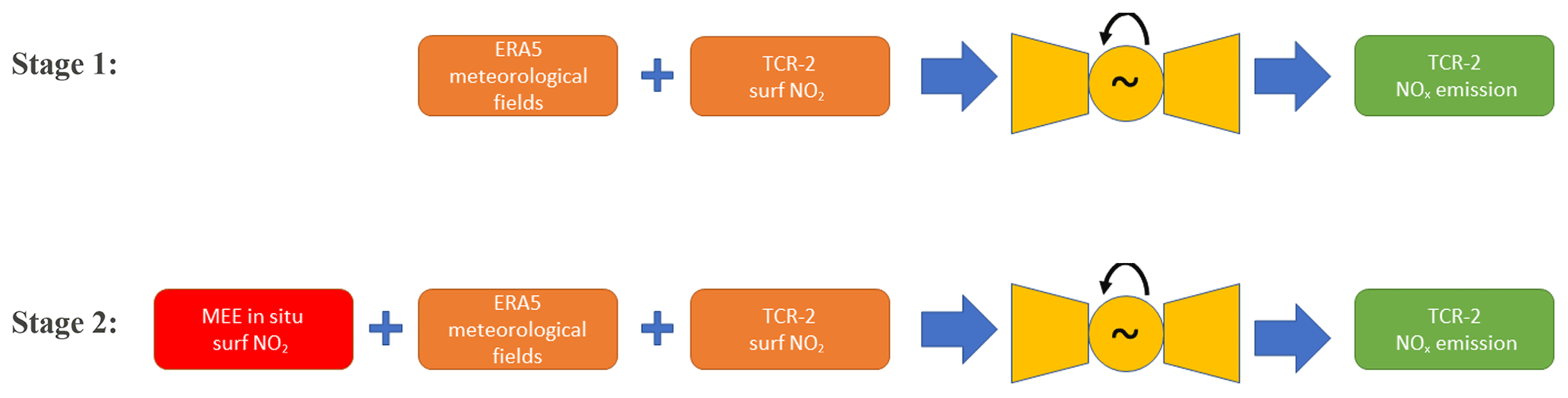
Figure 3 The two-stage training strategy used to integrate the in situ data with the TCR-2 data. In Stage 1, only the ERA5 meteorological fields and the TCR-2 surface NO₂ data (represented by the orange boxes) are used as predictors in training the model (indicated by the yellow symbols) to predict NO_x emissions (indicated by the green box). In Stage 2, the two surface NO₂ predictors (for days t and t−1) are replaced by the MEE in situ NO₂ measurements (denoted by the red box) with data gaps filled with the TCR-2 NO₂. Meteorological variables remain the same in both training stages.

Figure 4 Annual mean (a) TCR-2 surface NO₂, (b) MEE surface NO₂ with data gaps filled by TCR-2, and (c) TCR-2 NO_x emissions for 2019. East China is mostly covered by MEE, but West China has fewer stations and is mostly filled with TCR-2 data in (b).

3 Results and discussion

3.1 Analysis of the DL emission in 2019, during the testing period

A comparison of the Stage-1 DL analysis and the TCR-2 NO_x emissions for 2019 is shown in Fig. 5. The DL-estimated daily NO_x emissions are in good agreement with the TCR-2 “truth” after the first training stage, with a correlation coefficient of 0.96 and a slope of 1.02. The annual mean errors in the DL-estimated NO_x emissions are within 10 %. These results indicate that the DL model captured well the relationship between surface NO₂ and NO_x emissions from TCR-2 after the first training stage. The time series of estimated NO_x emissions for three metropolitan regions, five selected provinces, and four major cities in China are plotted in Fig. 6. As can be seen after Stage 1, the DL model agrees well with the TCR-2 emissions in most regions. Even on small scales such as Beijing, which is only one grid box at the 1.1^∘ resolution, the inferred emissions after Stage 1 are consistent with the TCR-2 emissions. The largest discrepancies after Stage 1 are found in the coastal regions of the Pearl River Delta (PRD) and the Yangtze River Delta (YRD), which encompass the cities of Guangzhou and Shanghai, respectively, (see Fig. 1 for the locations of the PRD and YRD regions).

Figure 5 Correlation between daily NO_x emissions from the TCR-2 estimates and the DL analysis for 2019 (the testing period).

The difficulty of the DL model in reproducing the TCR-2 emissions in the coastal regions, particularly in the PRD, could reflect issues in both TCR-2 and the DL model. In the coastal regions in southern China, cloud cover will result in significantly reduced observational coverage from the satellites, which would impact TCR-2. For example, in the PRD (and Guangzhou), TCR-2 exhibits periods, such as around days 50 and 100, with anomalously low and constant NO_x emissions, which could be due to reduced observational coverage. In addition, although both the PRD and the YRD experience heavy rainfall during the monsoon season, Luo et al. (2013) found that the PRD experience more frequent mesoscale convective systems and greater rainfall accumulation than the YRD, which they attributed to the mountainous topography of the PRD and the nearby ocean, in contrast to the more flat YRD. It is possible that at a resolution of $\mathrm{1.1}{}^{\circ }\times \mathrm{1.1}{}^{\circ }$, both TCR-2 and the DL model cannot capture the complex meteorology (e.g. the sea breeze circulation and its model errors) in the PRD and its impact on the trace gas distribution, and thus are unable to reproduce the appropriate relationship between the NO_x emissions and the atmospheric NO₂ concentrations.

After Stage 2, the NO_x emissions calculated by the DL model are still consistent with the TCR-2 emissions in the main source emission regions. For Jing-Jin-Ji (JJJ), the DL emissions are 13.8 % higher than the TCR-2 emissions, while for the YRD, the DL emissions are 10.0 % higher. The seasonal differences in the estimated emissions are given in Table 2. In JJJ, the differences between the DL and TCR-2 emissions are relatively constant throughout the year, whereas for the YRD the differences are small in autumn and larger in winter. In general, we find that the DL model suggests modest increases in emissions in central and eastern China, with relatively larger increases in the less-densely populated provinces, such as Sichuan. In Sichuan, the estimated DL emissions are 23.2 % higher than those in TCR-2 in summer. Comparison of the emissions after Stages 1 and 2 in Fig. 6 shows that these large increases were produced after incorporating the MEE data in Stage 2. Thus, it is helpful to compare the time series of the TCR-2 and MEE surface NO₂ data, which are plotted in Fig. 7. In Sichuan, the MEE observations suggest significantly higher surface NO₂ abundances, which could account for the higher DL emission estimates. For JJJ and the YRD, the TCR-2 NO₂ is in good agreement with the MEE data.

To further evaluate the estimated NO_x emissions, in Fig. 8 we compare the 2019 TRC-2 and DL emissions with the recently updated Multi-resolution Emission Inventory for China (MEIC) (Zheng et al., 2021). For total Chinese emissions, there is good consistency between the three inventories, with TCR-2, the DL model, and MEIC suggesting total Chinese emissions of 18.5 ± 3.9, 19.4, and 20.9 Tg NO, respectively. However, despite the good agreement on the national scale, there are regional differences between the inventories. Compared to TCR-2, MEIC suggested higher NO_x emissions in JJJ and in the Jiangsu province (the northeastern part of the YRD). The DL-estimated emissions are higher than TCR-2 in these regions, but lower than those of MEIC. In Inner Mongolia, both TCR-2 and the DL model infer higher emissions than MEIC, with the DL model suggesting more emissions than MEIC and less than TCR-2. For the PRD, TCR-2 NO_x emissions are slightly lower than MEIC, whereas the DL results are slightly higher than MEIC. In less-densely populated regions, such as Sichuan and Yunnan provinces, the DL-estimated NO_x emissions are higher than both TCR-2 and MEIC.

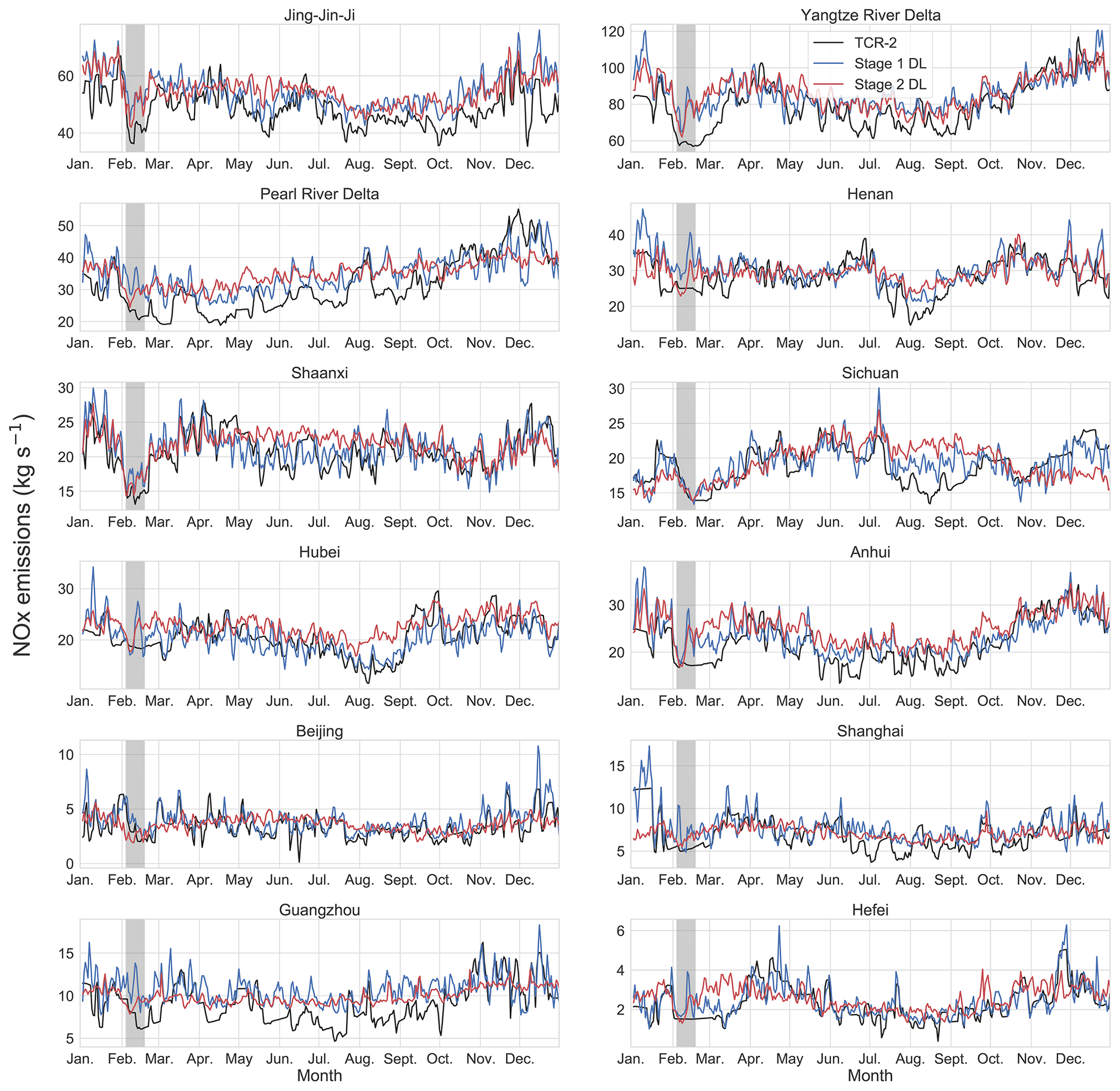
Figure 6 Time series of daily mean NO_x emissions in 2019 for three Chinese metropolitan regions (Jing-Jin-Ji, the Yangtze River Delta, and the Pearl River Delta), five selected provinces (Henan, Shaanxi, Sichuan, Hubei, and Anhui), and four major cities (Beijing, Shanghai, Guangzhou, and Hefei) for 2019 (the testing period). Shown are the emissions from the TCR-2 estimates (black) and the DL analysis after Stage 1 (blue) and Stage 2 (red). The shaded areas represent the 14 d period after the Chinese New Year.

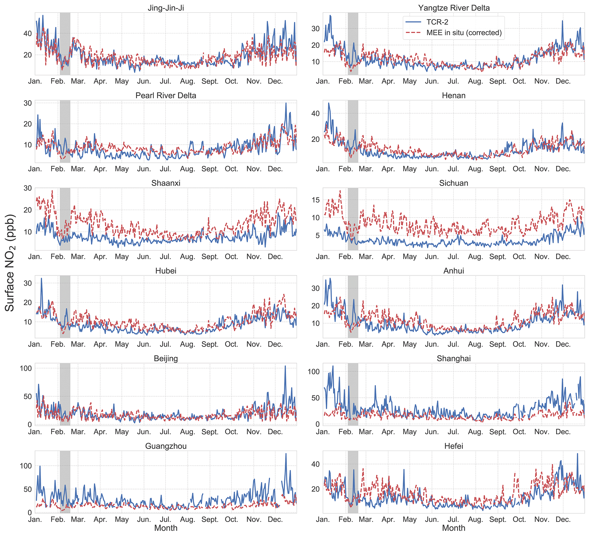
Figure 7 Time series of daily mean surface NO₂ concentrations in 2019 for the three Chinese metropolitan regions, selected provinces, and major cities shown in Fig. 6. The corresponding TCR-2 NO₂ data sampled at MEE sites are shown in blue, whereas the MEE ground-based NO₂ observations are indicated by the dashed red line. The shaded areas represent the 14 d period after the Chinese New Year.

Table 2 Mean percentage difference between the estimated seasonal NO_x emissions from the DL model (after Stage 2) and TCR-2 for 2019. Positive values represent that DL emissions are higher.

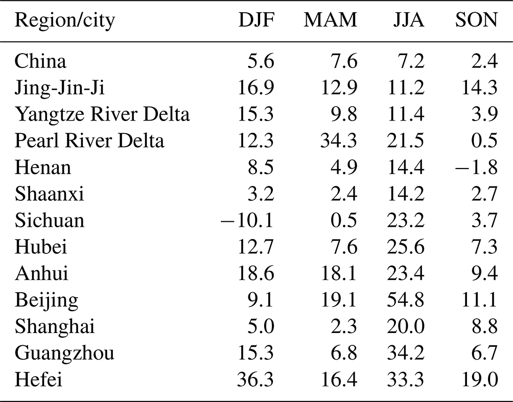
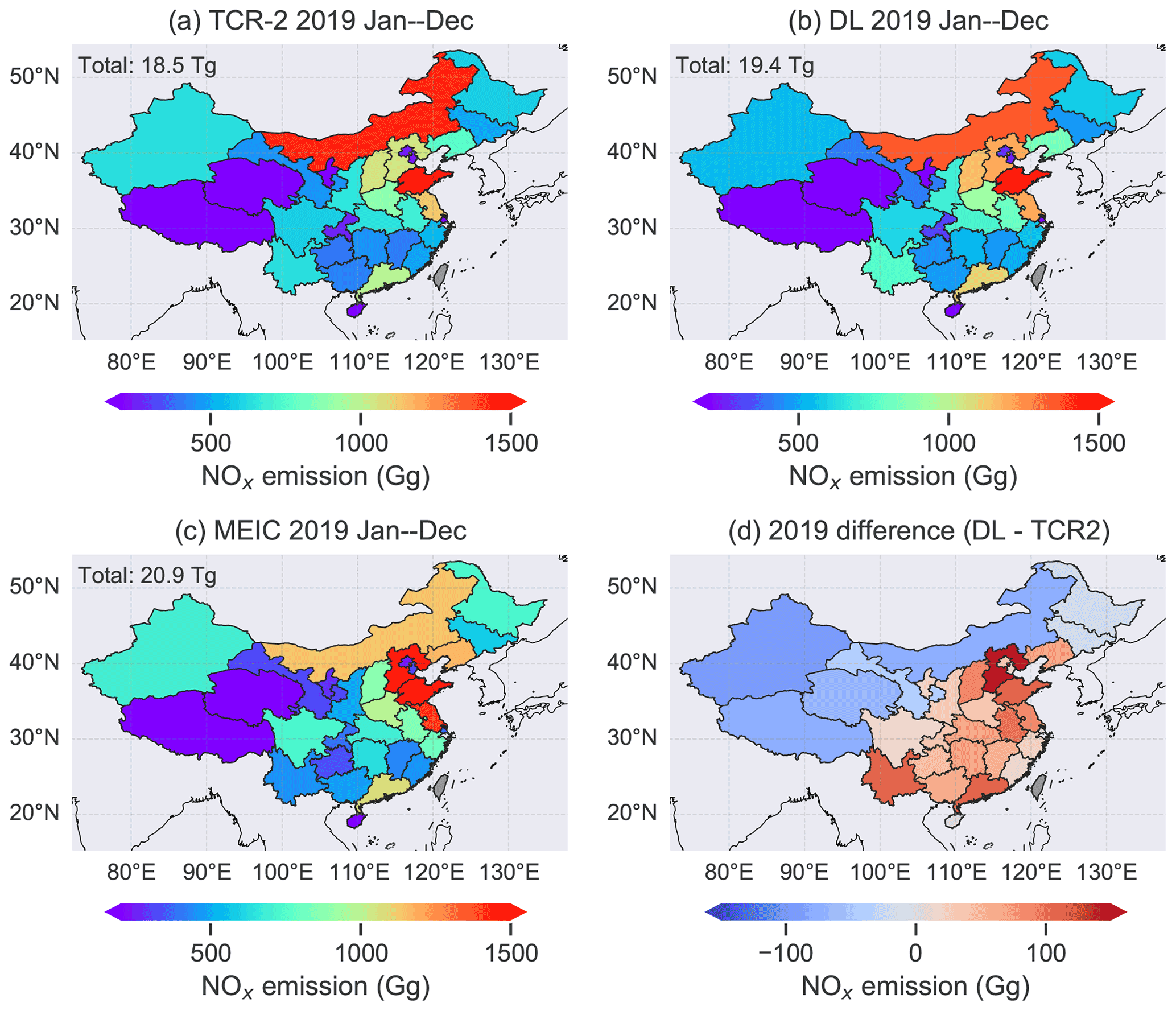
Figure 8 Annual NO_x emissions (Tg NO) for 2019 estimated by (a) the TCR-2 T106 data product, (b) the DL analysis and (c) the MEIC inventory. The DL minus TCR-2 emission differences are shown in (d).

3.2 Recovery of NO_x emissions after the Chinese New Year (CNY) holiday in 2019

Chinese NO_x emissions typically decrease around January and February every year due to reduced human activity during the Chinese New Year (CNY) holidays. After the 1-week holiday, Chinese NO_x emissions gradually recover to pre-holiday levels. This annual variation in NO_x emissions is well captured by TCR-2, as shown in Fig. 9. Starting from 10 d before the holidays, the Chinese NO_x emissions decrease rapidly by 20 % relative to emissions 20 d before the CNY, reaching a minimum shortly after the CNY. The interannual spread in TCR-2 emissions was about ±5 % for the 2005–2019 period, as similarly demonstrated by Miyazaki et al. (2020b), and the 2019 NO_x emissions were consistent with the multi-annual mean. The CNY-related variation in NO_x emissions was captured in TCR-2 in all three of the mega-regions: Jing-Jin-Ji (JJJ), the Yangtze River Delta (YDR), and the Pearl River Delta (PRD).

The DL analysis from Stage 2 was in good agreement with the TCR-2 emission estimates before the 2019 CNY for China and for the JJJ and YRD regions. However, after the holiday, the DL-based NO_x emissions recovered 50 % of the post-holiday reductions within 10–20 d, which was faster than in TCR-2 NO_x. The faster recovery in the DL-based NO_x emissions can be clearly seen for China and the YRD. The largest discrepancy between the DL model and TCR-2 was for the PRD region, where the variations in the DL-based NO_x emissions did not match that in TCR-2 before nor after the CNY. For example, TCR-2 exhibited large variations in the emissions, which the DL model does not capture. As discussed above, the DL model has difficulty reproducing the TCR-2 emissions in the PRD throughout 2019, even after Stage 1 of the training, when the model is trained solely on TCR-2 data, so the discrepancy between TCR-2 and the DL model in the signal of the CNY in the PRD emissions is consistent with the results shown in Fig. 6.

To validate the faster post-holiday recovery in the DL-based NO_x emissions, we use the C-index from the Baidu “Qianxi” data, which is also shown in Fig. 9. During the 2019 CNY period, the average C-index over the whole country rapidly decreased by 10 % from 4.5 to 4.1. It should be noted that the relationship between the C-index and NO_x emissions is not linear, as a 20 % decrease in NO_x emissions does not necessarily correspond to a comparable decrease in the C-index. However, as a measure of human activity and a proxy for NO_x emissions, the timing of the recovery in the C-index could provide useful information to evaluate the performance of the models in capturing the relative variations in NO_x emissions, especially from transportation source sectors. As shown in Fig. 9, the faster recovery of the DL model is consistent with the C-index. This is particularly evident for China, JJJ, and the YRD. Figure 10 shows the estimated time (in days) for the DL model, the TCR-2 NO_x emissions, and the C-index to recover to 50 % of the averaged values 5 d before the CNY for China, the three Chinese mega-regions, and all Chinese provinces. For all provinces, the recovery of the C-index took 9.5±5.2 d after the CNY (Fig. 10b). In comparison, the recovery of the NO_x emissions in the DL model and TCR-2 took 14.4±8.4 and 23.0±11.1 d, respectively. For JJJ and the YRD, the DL model suggested a recovery time of 15 and 16 d, respectively, whereas the C-index recovery took 9 d (Fig. 10a). For the PRD, the DL model recovered after 15 d, whereas the C-index recovered after 18 d.

The validation of the DL estimates here provide insights about the limitations of the satellite-derived NO_x emissions. Insufficient space-based observational constraints can limit the representation of short-term changes in NO_x emissions. The OMI observational coverage is limited, especially during winter over China due to cloudy or rainy conditions, and the relatively large retrieval uncertainty could prevent rapid a posteriori emission changes in the top-down analysis. This limitation could be mitigated by further optimization of the background error covariances in the top-down analysis to better reflect individual measurements. In addition, the use of more dense and accurate observations, such as from TROPOMI (see Sect. 3.3) could provide an improved representation of daily emission changes.

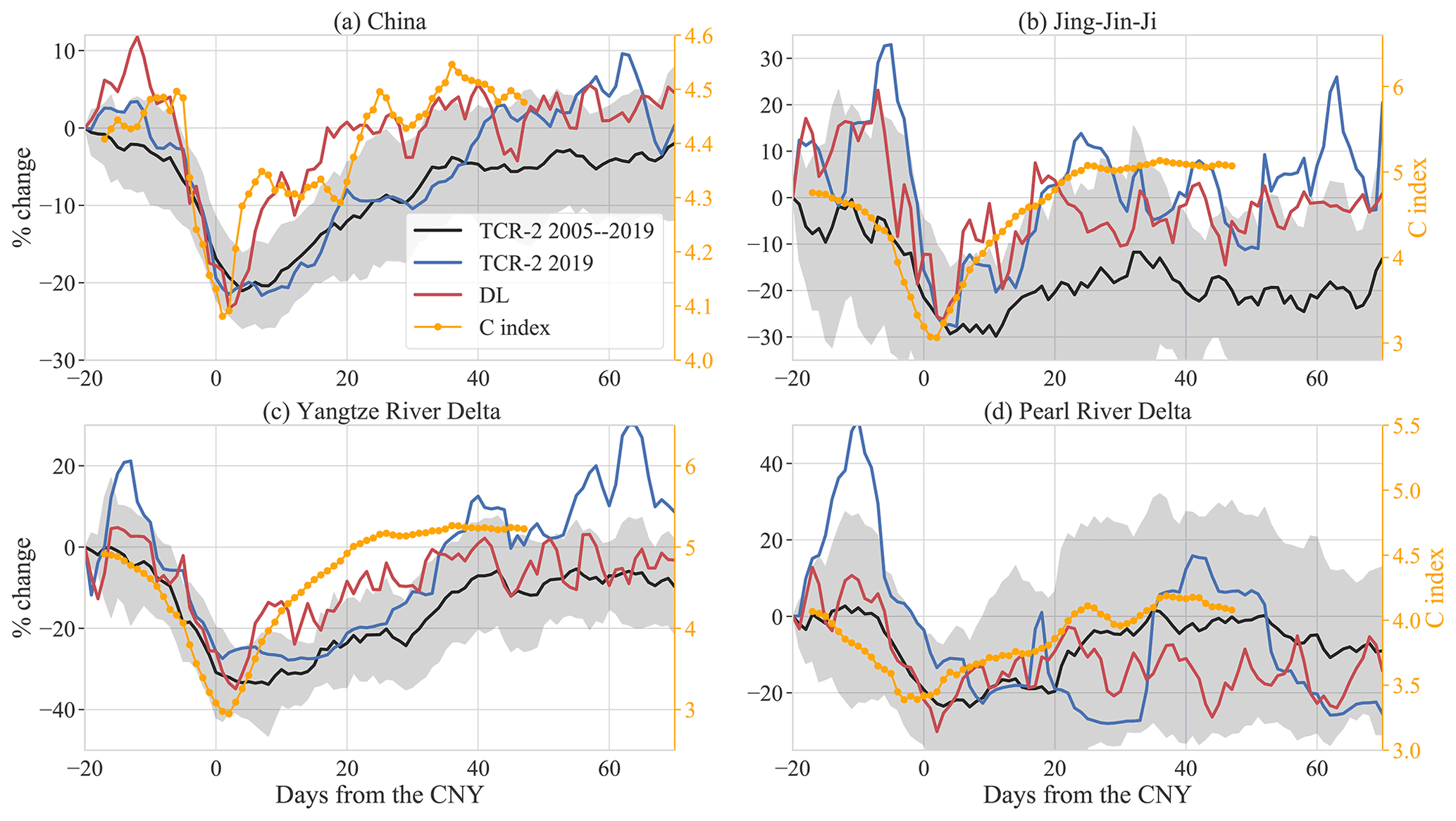
Figure 9 Time series of the percentage change in Chinese NO_x emissions and the C-index Baidu mobile data as a function of days from the CNY. The differences are plotted relative to 20 d before the 2019 CNY. Shown are time-series comparisons for (a) China, (b) the Jing-Jin-Ji region, (c) the Yangtze River Delta region, and (d) the Pearl River Delta region. The black line represents the TCR-2 mean for 2005–2019. The C-index is smoothed by a 7 d window to remove weekly variability.

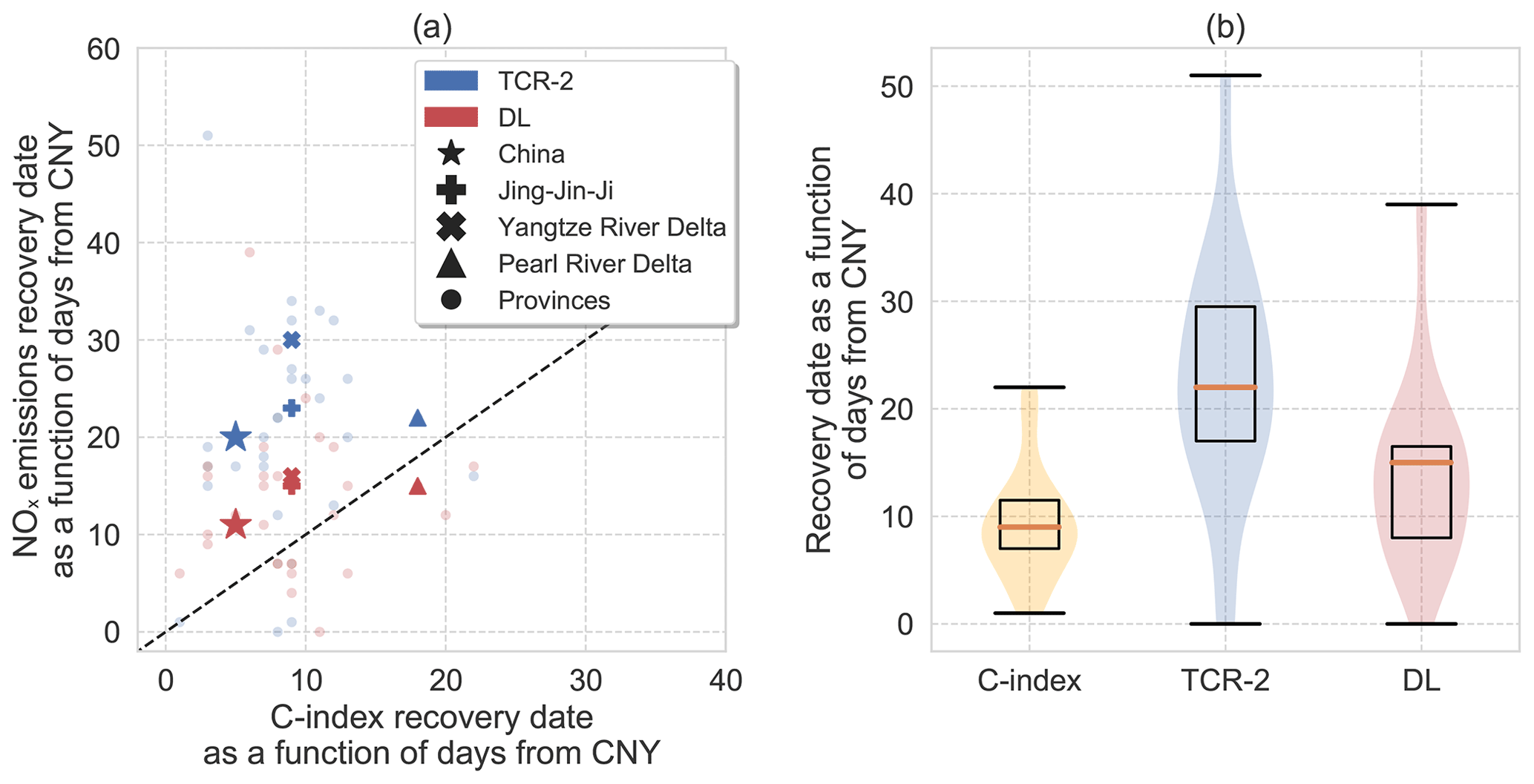
Figure 10 Comparison of the timing of the recovery of the NO_x emissions and Baidu C-index data back to 50 % of the averaged values 5 d before the CNY in 2019. (a) The scatter plot of NO_x emission recovery dates versus the C-index recovery dates. Each circle represents a province and special markers correspond to the larger regions as indicated by the legend. (b) Box whisker plots and the normalized distribution of the recovery dates for the C-index, TCR-2 NO_x emissions, and the DL-based NO_x emissions, calculated based on all provinces in China.

3.3 Analysis of the 2020 COVID-19 pandemic period

Since the COVID-19 pandemic lockdown led to a significant and unexpected perturbation to human activity, we examine the ability of the DL model to quantify changes in NO_x emissions during the lockdown period in China in 2020. Here we use the TROPOMI-based higher-resolution analysis using TCR-2 (hereafter referred to as T213 data) as an independent data set for the evaluation of the DL model. The standard OMI-based TCR-2 data product is hereafter referred to as T106 data. The T213 data were used to study detailed spatial and temporal changes in NO_x emissions during the COVID-19 lockdown period (Miyazaki et al., 2020b, 2021). The T213 product is expected to better capture variability in NO_x emissions, compared to the T106 product, because of the greater observational constraints from TROPOMI and the higher spatial resolution and coverage. The time series of the relative changes in NO_x emissions around the 2020 CNY are shown in Fig. 11. We choose the reference date to be 10 d before the 2020 CNY to avoid spin-up issues in the T213 data. On the national scale, all three NO_x emission estimates decreased at roughly the same rate until about 10 d after the 2020 CNY, after which the DL-based emission began increasing. The T106 and T213 NO_x emissions continued to decrease for about an additional 10 d after the CNY, with the T213 data suggesting a smaller overall reduction than T106. All three NO_x emission estimates suggested that a full recovery took 60 d after the CNY. However, of the three, the DL-based estimates suggested the smallest overall reduction in Chinese NO_x emissions. For JJJ, the DL-based and T106 emissions estimates were fairly consistent, but the T213 estimates suggested a faster recovery.

Comparison of the NO_x emission time series with the C-index in Fig. 11 shows distinct differences in the timing of the minimum in the data after the 2020 CNY. As noted above, we do not expect there to be a linear relationship between the C-index and the NO_x emissions, but since the reduction in emissions is in part driven by the lockdown, we anticipate that the minimum in the migration data should closely correspond to the minimum in emissions. For China, as listed in Table 3, the C-index reached a minimum 14 d after the CNY, whereas the DL model, the T213 data, and the T106 data reached a minimum within 13, 21, and 23 d, respectively. The DL model reproduced well the timing of the minimum for JJJ and the YRD. However, it significantly underestimated the timing for the PRD (3 d for the DL model compared to 12 d for the C-index). But as we noted above, the DL model has difficulty simulating the PRD, and the timing of the minimum for the PRD is not well defined, as the signal is noisy and exhibits a fairly broad minimum. We find that the timing of the minima in the T213 emissions more closely match that of the C-index than T106, which suggested delayed minima.

The timing of the recovery of the post-holiday reductions to 50 % of the averaged values 5 d before the holiday for the C-index and the estimated NO_x emissions are listed in Table 4. For China, the C-index took 31 d to recover in 2020, whereas the DL model and the T213 data took 31 and 37 d, respectively, to recover. The recovery time in T106 data was 41 d. For JJJ, the time required for the 50 % recovery was 34 d for the C-index, whereas for the DL model, the T213 data, and the T106 data it was 34, 36, and 31 d, respectively. For the YRD, both reanalysis data products took over 40 d to recover, which is more than 20 d longer than the C-index and more than 10 d longer than the DL model. In the PRD, all of the estimated NO_x emissions took more than 20 d longer to recover than the C-index.

The spatial distribution of the DL-estimated changes in Chinese NO_x emissions 20–30 d after the 2020 CNY, relative to 10–20 d prior to the CNY, are shown in Fig. 12. The DL analysis shows over 30 % reduction in NO_x emissions 20–30 d after the 2020 CNY for the heavily polluted regions in northern and eastern China. In JJJ, the DL analysis suggested a maximum reduction in NO_x emissions of 42 % during the lockdown period, whereas the T106 and T213 data indicated a maximum reduction of 49 % and 41 %, respectively. Using a regional model to assimilate the MEE data to estimate NO_x emissions for January–March 2020, Feng et al. (2020) estimated a reduction of 42 % in NO_x emissions for JJJ. For the YRD, the DL model and the T106 data suggested comparable reductions of 30 % and 31 %, respectively, which were roughly 10 % smaller than the reductions in the T213 data and in Feng et al. (2020) of 40 % and 41 %, respectively. The comparison here shows that the impact of the lockdown on NO_x emissions in the higher-resolution T213 data, in contrast to the T106 data, is more consistent with Feng et al. (2020). This confirms that the emission analysis at T106 resolution (1.1^∘) constrained by the OMI measurements may not provide sufficient information to capture rapid regional variations in NO_x emissions. The four analyses exhibited the largest disagreement in the PRD, where Feng et al. (2020) estimated a 50 % maximum reduction in emissions, whereas the T106 and T213 data suggested maximum reductions of 39 % and 35 %, respectively. The DL model significantly underestimated the emission reduction in the region, with a maximum reduction of 24 %. Overall, the comparison with the migration data and with the Feng et al. (2020) results indicate that, with the exception of the PRD, integrating the MEE and TCR-2 data results in an improved relationship between surface NO₂ concentrations and NO_x emissions.

Table 3 Timing (in days) of the minimum in the migration data and NO_x emissions during 30 d after the 2020 CNY.

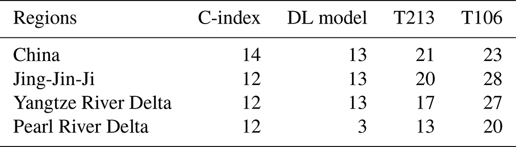
Table 4 Time (in days) for the migration data and NO_x emissions to recover to 50 % of the pre-CNY level in 2020.

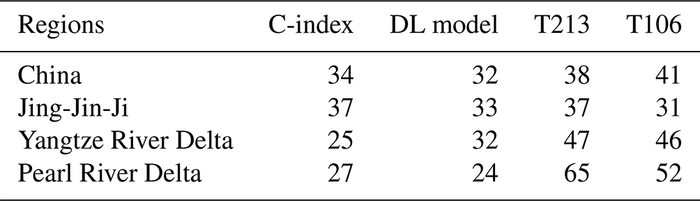
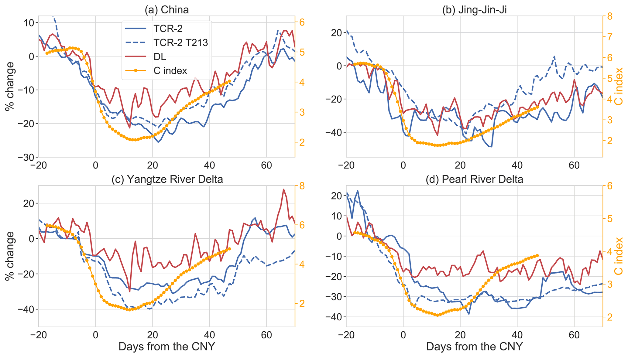
Figure 11 Time series of percentage changes in NO_x emissions and the C-index Baidu mobility data, relative to 10 d before the 2020 CNY, as a function of days from the CNY. Shown are the time series for (a) China, (b) the Jing-Jin-Ji region, (c) the Yangtze River Delta, and (d) the Pearl River Delta.

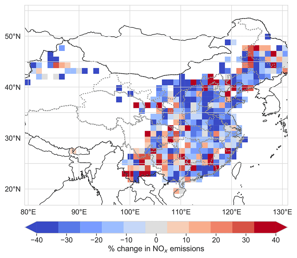
Figure 12 DL-estimated percent changes in Chinese NO_x emissions averaged 20–30 d after the 2020 CNY compared to 20–10 d before the 2020 CNY. Results for grid boxes with NO_x emissions less than $\mathrm{1}\times {\mathrm{10}}^{-\mathrm{11}}$ kgN m⁻² s⁻¹ are not shown.

4 Conclusions

We developed a DL model to estimate Chinese NO_x emissions using surface NO₂ concentration and meteorological predictors, based on the integration of MEE in situ NO₂ observations with TCR-2 NO₂. To that end, we applied a multistage training strategy for the transfer learning of the chemical relationship between surface NO₂ and NO_x emissions in the TCR-2 data set. We found that the integration of the MEE in situ data with TCR-2 suggested NO_x emissions from China for 2019 to be 19.4 Tg NO, which is consistent with the 18.5 ± 3.9 Tg NO estimated by TCR-2. The DL model and TCR-2 were both consistent with the suggested Chinese source of 20.9 Tg NO in the MEIC inventory (Zheng et al., 2021). For the JJJ and YRD mega-regions in China, the DL-based NO_x emissions were higher than TCR-2 by 13.8 % and 10.0 %, respectively. The DL model particularly increased emissions in the less-densely populated provinces, where the MEE observations indicated higher surface NO₂ abundances than in TCR-2. He et al. (2022) suggested that inversions using satellite observations to estimate NO_x emissions have the potential to blend information from background NO_x and surface emissions at coarse spatial resolutions. It is possible that much higher resolution than the $\mathrm{1.1}{}^{\circ }\times \mathrm{1.1}{}^{\circ }$ of TCR-2 is needed for the satellite-based assimilation system to capture the surface NO₂ signal in these less-densely populated provinces. We also found that the DL model could not reproduce the TCR-2 relationship between NO_x emissions and surface NO₂ in the PRD, and integration of the MEE data resulted in large adjustments in the NO_x emissions in the region. During the monsoon season, southern China experiences heavy and frequent rainfall, and the mountainous topography of the PRD and its proximity of the ocean could make it challenging for TCR-2 and the DL model to accurately account for the influence on surface NO₂ of the complex meteorology in the region at a resolution of $\mathrm{1.1}{}^{\circ }\times \mathrm{1.1}{}^{\circ }$.

Analysis of the DL-based NO_x emissions focused around the CNY holiday in 2019 showed a faster recovery of the Chinese NO_x emissions after the 2019 CNY, which was consistent with the Baidu “Qianxi” mobile data (Kraemer et al., 2020; Zhang et al., 2021). During the 2020 lockdown period for the COVID-19 pandemic, the DL model estimated maximum reductions in NO_x emissions – 42 % for JJJ and 30 % for the YRD. These estimates were consistent with the TCR-2 T106 data (with reductions of 49 % for JJJ and 31 % for the YRD), the high-resolution TCR-2 T213 data (with reductions of 41 % for JJJ and 40 % for the YRD), and with Feng et al. (2020) (who estimated reductions of 42 % for JJJ and 41 % for the YRD). For the PRD, the DL model estimated a significantly smaller maximum reduction in NO_x emissions of 24 %, which is likely due to the model bias in the region.

The analysis during the 2020 lockdown period showed that the DL model has the ability to extrapolate outside the regime of the training data set. Our results showed the potential of this DL model as a good complementary tool for conventional data-assimilation approaches. The flexibility of the model is such that it could be adapted to provide near-real time estimates of NO_x emissions for air quality forecasts and chemical reanalysis systems. The high computational efficiency of the DL model in integrating large amounts of observational data from multiple sources would be advantageous in the emerging era with geostationary satellites that will significantly enhance observational coverage for air quality applications.