Decay times of atmospheric acoustic–gravity waves after deactivation of wave forcing

High-resolution numerical simulations of non-stationary, nonlinear acoustic–gravity waves (AGWs) propagating upwards from surface wave sources are performed for different temporal intervals relative to activation and deactivation times of the wave forcing. After activating surface wave sources, amplitudes of AGW spectral components reach a quasi-stationary state. Then the surface wave forcing is deactivated in the numerical model, and amplitudes of vertically traveling AGW modes quickly decrease at all altitudes due to discontinuations of the upward propagation of wave energy from the wave sources. However, later the standard deviation of residual and secondary wave perturbations experiences a slower quasi-exponential decrease. High-resolution simulations allowed, for the first time, for the estimation of the decay times of this wave noise produced by slow residual, quasi-standing and secondary AGW spectral components, which vary between 20 and 100 h depending on altitude and the rate of wave source activation and deactivation. The standard deviations of the wave noise are larger for the case of sharp activation and deactivation of the wave forcing compared to the steep processes. These results show that transient wave sources may create long-lived wave perturbations, which can form a background level of wave noise in the atmosphere. This should be taken into account in parameterizations of atmospheric AGW impacts.

1 Introduction

Recently, acoustic–gravity waves (AGWs) are believed to exist almost permanently in the atmosphere (Siefring et al., 2010; Snively et al., 2013; Wei et al., 2015; Lay, 2018; Meng et al., 2019). Observations detect regular AGW presence up to high atmospheric altitudes (e.g., Djuth et al., 2004; Park et al., 2014; Trinh et al., 2018). Modeling of general circulation demonstrated AGW capabilities of transferring energy and momentum from tropospheric wave sources to higher atmospheric levels (e.g., Medvedev and Yiğit, 2019). Nonhydrostatic models of the general circulation of the atmosphere revealed that AGWs permanently exist at all atmospheric heights (e.g., Yiğit et al., 2012).

Many AGWs detected in the atmosphere are excited in the troposphere (Fritts and Alexander, 2003; Snively, 2013; Yiğit and Medvedev, 2014). AGWs can be produced by interactions of winds with mountains (e.g., Gossard and Hooke, 1975), atmospheric jet streams and fronts (e.g., Gavrilov and Fukao, 1999; Dalin et al., 2016), thunderstorms and cumulus clouds (Siefring et al., 2010; Blanc et al., 2014; Lay, 2018), convective regions and shear flows (Townsend, 1966; Fritts and Alexander, 2003; Vadas and Fritts, 2006), typhoons (Wu et al.,2015), volcanoes (De Angelis et al., 2011), waves on the sea surface (Godin et al., 2015), explosions at the Earth's surface (Meng, 2019), earthquakes (Rapoport et al., 2004), tsunamis (Wei at al., 2015), different objects moving in the atmosphere (Afraimovich et al., 2002), big fires, etc. Some AGWs can be generated by mesoscale turbulence in the atmosphere (Townsend, 1965; Medvedev and Gavrilov, 1995). These AGW sources are located mainly at tropospheric heights (Gavrilov and Fukao, 1999; Dalin, 2016).

Most wave sources listed above are non-stationary. They can be activated during initial time intervals, operate for some time and then be deactivated during final time intervals. The initial and final time intervals could be shorter or longer depending on the physical properties of particular wave sources. Non-stationary activating and deactivating wave sources can generate transient AGW pulses propagating upwards from the lower atmosphere, which require their analysis.

High-resolution numerical models are frequently used for studies of meso- and microscale processes in the atmosphere, for example, the Weather Research and Forecasting Nonhydrostatic Mesoscale Model, also known as the North American Mesoscale Model (WRF, 2019), as well as the Regional Atmospheric Modeling System (RAMS) described by Pielke et al. (1992) and other similar models. Direct numerical simulation (DNS) and large-eddy simulation (LES) models (e.g., Mellado, 2018) should be mentioned in this context. Fritts et al. (2009, 2011) used a numerical model of Kelvin–Helmholtz instabilities, AGW breaking and generation of turbulence in atmospheric regions with fixed horizontal and vertical extents. They utilized a Galerkin-type algorithm for turning partial differential equations into equations for spectral series coefficients. Liu et al. (2009) simulated the propagation of atmospheric AGWs and creation of Kelvin–Helmholtz billows. Yu et al. (2017) used a numerical model for AGWs propagating in the atmosphere from tsunamis.

Gavrilov and Kshevetskii (2013) studied nonlinear AGWs with a numerical two-dimensional model, which involved fundamental conservation laws. This model permitted non-smooth solutions of the nonlinear wave equations and gave the required stability of the numerical model (Kshevetskii and Gavrilov, 2005). A respective three-dimensional algorithm was introduced by Gavrilov and Kshevetskii (2014) to simulate nonlinear atmospheric AGWs. Gavrilov and Kshevetskii (2013, 2014) showed that after triggering wave forcing at the lower boundary of the numerical model, initial AGW pulses could reach high atmospheric levels in a few minutes. AGW phase surfaces are quasi-vertical initially, but later they become inclined to the horizon. AGW vertical wavelengths decrease in time and are close to their theoretical predictions after intervals of a few periods of wave forcing.

In this study, using the high-resolution nonlinear wave model developed by Gavrilov and Kshevetskii (2014), we continue simulating transient waves generated by non-stationary AGW sources at the lower boundary and propagating upwards to the atmosphere. The main focus is AGW behavior after deactivations of wave sources in the model. After activating the surface wave source and disappearing initial wave pulses, AGW amplitudes tend to stabilize at all atmospheric altitudes. In this quasi-stationary state, the surface wave forcing is deactivated in the numerical model. After that, amplitudes of traveling AGW modes quickly decrease at all altitudes due to discontinuation of the upward propagation of wave energy from the surface sources. We found, however, that after some time, the standard deviation of residual quasi-standing and secondary wave perturbations experiences a slower exponential decrease with substantial decay times.

These results show that residual and secondary AGW modes produced by transient wave sources can exist for a long time in the stratosphere and mesosphere and form a background level of wave noise there. AGW decay times and their dependences on parameters of the surface wave forcing are estimated for the first time.

2 Numerical model

In this study, we employed the high-resolution three-dimensional numerical model of nonlinear AGWs in the atmosphere developed by Gavrilov and Kshevetskii (2014). Currently, this model (called AtmoSym) is available for free online usage (AtmoSym, 2017). The AtmoSym model utilizes the plain geometry and primitive hydrodynamic three-dimensional equations (Gavrilov and Kshevetskii, 2014):

$$\begin{array}{}\text{(1)}& \begin{array}{rl}& {\displaystyle \frac{\partial \mathit{\rho }}{\partial t}}+{\displaystyle \frac{\partial \mathit{\rho }{v}_{\mathit{\beta }}}{\partial x_{\mathit{\beta }}}}=\mathrm{0},\mathit{\rho }{c}_p{\displaystyle \frac{\mathrm{d}T}{\mathrm{d}t}}={\displaystyle \frac{\mathrm{d}p}{\mathrm{d}t}}+\mathit{\rho }\mathit{\epsilon },p=\mathit{\rho }RT,\\ & {\displaystyle \frac{\partial \mathit{\rho }{v}_i}{\partial t}}+{\displaystyle \frac{\partial \mathit{\rho }{v}_i{v}_{\mathit{\beta }}}{\partial x_{\mathit{\beta }}}}=-{\displaystyle \frac{\partial p}{\partial x_i}}-\mathit{\rho }g{\mathit{\delta }}_{i\mathrm{3}}+{\displaystyle \frac{\partial {\mathit{\sigma }}_{i\mathit{\beta }}}{\partial x_{\mathit{\beta }}}},i,\mathit{\beta }=\mathrm{1},\mathrm{2},\mathrm{3},\end{array}\end{array}$$

where t is time; p, ρ and T are pressure, density and temperature, respectively; v_β represents the velocity components along the coordinate x_β axes; σ_iβ is the viscous stress tensor; g is the acceleration due to gravity; c_p is the specific heat capacity at constant pressure; R is the atmospheric gas constant; ε is the specific heating rate; $\mathrm{d}/\mathrm{d}t$ = $\partial /\partial t+v_{\mathit{\beta }}\partial /\partial x_{\mathit{\beta }}$; repeating Greek indexes assume summation. Quantities σ_iβ and ε in Eq. (1) contain stresses and heating rates produced by molecular viscosity and heat conductivity (see details in Gavrilov and Kshevetskii, 2014). After numerical integration of Eq. (1), dynamical deviations (marked with primes below) from stationary background values p₀, ρ₀, T₀ and v_i0 are calculated:

$$\begin{array}{}\text{(2)}& p^{\prime }=p-p_{\mathrm{0}};{\mathit{\rho }}^{\prime }=\mathit{\rho }-{\mathit{\rho }}_{\mathrm{0}};T^{\prime }=T-T_{\mathrm{0}};{v^{\prime }}_i=v_i-v_{i\mathrm{0}}.\end{array}$$

The AtmoSym model takes into account dissipative and nonlinear processes that accompany AGW propagation. The model is capable of simulating such complicated processes as AGW instability, breaking and turbulence generation. Dynamical deviations as defined in Eq. (2) describe both wave perturbations and modifications of background fields due to momentum and energy exchange between dissipating AGWs and the atmosphere. The background temperature T₀(z) is obtained from the semi-empirical NRLMSISE-00 atmospheric model (Picone et al., 2002). Background dynamic molecular viscosity, μ₀, and heat conductivity, κ₀, are estimated using Sutherland's formulae (Kikoin, 1976):

$$\begin{array}{}\text{(3)}& \begin{array}{rl}& {\mathit{\mu }}_{\mathrm{0}}={\displaystyle \frac{\mathrm{1.46}\times {\mathrm{10}}^{-\mathrm{6}}\sqrt{T_{\mathrm{0}}}}{\mathrm{1}+\mathrm{110}/T_{\mathrm{0}}}}\left({\displaystyle \frac{\mathrm{kg}}{\mathrm{m}\mathrm{s}}}\right)\\ & {\mathit{\kappa }}_{\mathrm{0}}={\displaystyle \frac{{\mathit{\mu }}_{\mathrm{0}}}{\text{Pr}}};\mathrm{\text{Pr}}={\displaystyle \frac{\mathrm{4}\mathit{\gamma }}{\mathrm{9}\mathit{\gamma }-\mathrm{5}}},\end{array}\end{array}$$

where γ is the heat capacity ratio, and Pr is the Prandtl number. The AtmoSym model also involves the mean turbulent thermal conductivity and viscosity having maxima of about 10 m² s⁻¹ in the boundary layer and in the lower thermosphere and a broad minimum of up to 0.1 m² s⁻¹ in the stratosphere (Gavrilov and Kshevetskii, 2014). The upper boundary conditions at z=h have the following form (Kurdyaeva et al., 2018):

$$\begin{array}{}\text{(4)}& \begin{array}{rl}& {\left({\displaystyle \frac{\partial T}{\partial z}}\right)}_{z=h}=\mathrm{0},{\left({\displaystyle \frac{\partial v_{\mathrm{1}}}{\partial z}}\right)}_{z=h}=\mathrm{0},{\left({\displaystyle \frac{\partial v_{\mathrm{2}}}{\partial z}}\right)}_{z=h}=\mathrm{0},\\ & (w{)}_{z=h}=\mathrm{0},\end{array}\end{array}$$

where indices 1 and 2 correspond to horizontal directions, and w=v₃ is vertical velocity. Conditions (Eq. 4) may cause reflections of AGWs coming from below. The upper boundary in the present study is set at h = 600 km, where molecular viscosity and heat conductivity are very high, and reflected waves are strongly dissipated. Sensitivity tests reveal that the impact of conditions at the upper boundary as defined by Eq. (4) is negligible at altitudes z < h−2H, where H is the atmospheric scale height. Therefore, at altitudes of the middle atmosphere analyzed in this paper, the influence of the upper boundary conditions (Eq. 4) could be negligible. The lower boundary conditions at the Earth's surface have the following form (see Kurdyaeva et al., 2018):

$$\begin{array}{}\text{(5)}& \begin{array}{rl}& (T^{\prime }{)}_{z=\mathrm{0}}=\mathrm{0},(v_{\mathrm{1}}{)}_{z=\mathrm{0}}=\mathrm{0},(v_{\mathrm{2}}{)}_{z=\mathrm{0}}=\mathrm{0},\\ & (w{)}_{z=\mathrm{0}}=W_{\mathrm{0}}\cos (\mathit{\sigma }t-\mathit{k}\cdot \mathit{r}),\end{array}\end{array}$$

where W₀ and σ are the amplitude and frequency of wave excitation; $\mathit{k}=(k_{\mathrm{1}},k_{\mathrm{2}})$ is the horizontal wave vector; $\mathit{r}=(x_{\mathrm{1}},x_{\mathrm{2}})$ is the position vector in the horizontal plane; and k₁ and k₂ are the wavenumbers along horizontal x₁ and x₂ axes, respectively. The last relation for the surface vertical velocity in Eq. (5) serves as the source of plane AGW modes in the AtmoSym model. Such plane modes can represent spectral components of tropospheric dynamical processes. Their effects can be approximated by appropriate sets of effective spectral components of vertical velocity at the lower boundary (Townsend, 1965, 1966). Along horizontal x₁ and x₂ axes, one can assume periodicity of wave fields

$$\begin{array}{}\text{(6)}& F(x_{\mathrm{1}},x_{\mathrm{2}},z,t)=F(x_{\mathrm{1}}+L_{\mathrm{1}},x_{\mathrm{2}}+L_{\mathrm{2}},z,t),\end{array}$$

where F denotes any of the simulated hydrodynamic quantities; L₁=n₁λ₁ and L₂=n₂λ₂ are horizontal dimensions of the analyzed atmospheric region; ${\mathit{\lambda }}_{\mathrm{1}}=\mathrm{2}\mathit{\pi }/k_{\mathrm{1}}$ and ${\mathit{\lambda }}_{\mathrm{2}}=\mathrm{2}\mathit{\pi }/k_{\mathrm{2}}$ are wavelengths along the x₁ and x₂ axes, respectively; and n₁ and n₂ are integers.

In our simulations, the wave excitation in Eq. (5) is activated at the moment t=t_a, and then its amplitude W₀ does not change for some time. One should expect that at small amplitudes of wave source in Eq. (5), the numerical solutions in the lower and middle atmosphere should tend at t≫t_a to a steady-state plane AGW mode corresponding to the traditional linear theory (e.g., Gossard and Hooke, 1975). Gavrilov et al. (2015) showed good agreement of ratios of simulated amplitudes of different wave fields with polarization relations of linear AGW theory (Gossard and Hooke, 1975) at t≫t_a at altitudes up to 100 km.

The novelty of the present study is deactivating the wave source in Eq. (5) at some moment t=t_d after reaching the quasi-steady solution described above. Previous simulations with the AtmoSym model showed that sharp activation of the surface wave source (Eq. 5) could create an initial AGW pulse, which can reach high altitudes in a few minutes. To control the rate of the wave source activation and deactivation, in the present simulations, we multiply the surface vertical velocity in Eq. (5) by a function

$$\begin{array}{}\text{(7)}& q\left(t\right)=\left\{\begin{array}{lll}\exp \left[-(t-t_{\mathrm{a}}{)}^{\mathrm{2}}/s_{\mathrm{a}}^{\mathrm{2}}\right]& \text{at}& t\le t_{\mathrm{a}}\\ \mathrm{1}& \text{at}& t_{\mathrm{a}}<t<t_{\mathrm{d}}\\ \exp \left[-(t-t_{\mathrm{d}}{)}^{\mathrm{2}}/s_{\mathrm{d}}^{\mathrm{2}}\right]& \text{at}& t\ge t_{\mathrm{d}}\end{array}\right\},\end{array}$$

where s_a and s_d are constants.

3 Results of numerical simulations

Our numerical modeling begins with a steady-state, windless, non-perturbed atmosphere with profiles of background temperature, density, molecular weight and molecular kinematic viscosity corresponding to January at latitude 50^∘ N at medium solar activity according to the NRLMSISE00 model (Picone et al., 2002), which are presented in Fig. 1 of the paper by Gavrilov et al. (2018).

Figure 1 Spectral density (in relative units) of the surface wave source (Eq. 5) having period of 2 h for 20 h running time intervals centered at model times t≈ 20 h (a), t≈ 70 h (b) and t≈ 120 h (c), which correspond to the wave forcing activation, activated state and deactivation. Solid and dashed lines correspond to the steep and sharp activation and deactivation rates s_a and s_d in (Eq. 7).

In this study, we consider AGW modes propagating along the eastward x axis and assume the horizontal dimension of the considered atmospheric region to be equal to the circle of latitude at 50^∘ N, which is L_x≈ 27 000 km. At horizontal boundaries of this circle of latitude, we use periodical boundary conditions according to Eq. (6). Representing the circle of latitude by a rectangle area assumes fixed L_x at all altitudes, while in spherical coordinates L_x is increasing in altitude. However, the differences in L_x at altitudes of the middle atmosphere do not exceed 2 %. Modeling was performed with the surface wave source (Eq. 5) for AGW modes with amplitudes W₀ = 0.01–0.1 mm s⁻¹. The smallest amplitudes correspond to weak AGWs, for which nonlinear effects are small at all considered altitudes. Excitations at W₀ ∼ 0.1 mm s⁻¹ produce strong AGWs with substantial nonlinear interactions in the mesosphere and lower thermosphere. The used range of horizontal phase speeds c_x ∼ 50–200 m s⁻¹ corresponds to AGW modes with relatively large vertical wavelengths, which can propagate from the ground up to the upper atmosphere. The number of wave periods along the circle of latitude is taken to be n₁=32. This corresponds to the horizontal wavelength of ${\mathit{\lambda }}_x=L_x/n_{\mathrm{1}}\approx$ 844 km and AGW periods of $\mathit{\tau }={\mathit{\lambda }}_x/c_x$ ∼ 4.7–1.2 h for the range of c_x values specified above. The horizontal grid spacing of the numerical model is $\mathrm{\Delta }x={\mathit{\lambda }}_x/\mathrm{16}$, and the time step of calculations was automatically adjusted to Δt≈ 2.9 s. The vertical grid of the model covers altitudes up to h = 600 km and contains 1024 non-equidistant nodes. Vertical spacing varies between 12 m and 3 km from the lower to the upper boundary, so about 70 % of the grid nodes are located in the lower and middle atmosphere.

For parameters of the smoothing factor (Eq. 7) in the present simulations, we take t_a = 10⁵ s ≈ 28 h and t_d = 4 × 10⁵ s ≈ 110 h and consider steep AGW source activating and deactivating with s_a=s_d = 3.3 × 10⁴ s ≈ 9 h and sharp triggering at s_a=s_d = 0.3 s. The shape of the smoothing factor (Eq. 7) influences the spectrum of the surface wave source in the model. Figure 1 shows spectra of the sinusoidal source (Eq. 5) with wave period τ = $\mathrm{2}\mathit{\pi }/\mathit{\sigma }$ = 2 h, which were calculated using 20 h running time intervals corresponding to the phases of activation, activated state and deactivation of the wave source (Eq. 5) with the abovementioned “steep” and “sharp” values of s_a and s_d in Eq. (7). Comparisons of solid and dashed lines in Fig. 1 show that the sharp activation and deactivation of the wave source decrease the spectral density at the frequency of the main spectral maximum. However, the sharp triggering considerably increases the high-frequency part of the wave spectra in Fig. 1, which means larger proportions of acoustic waves generated by quickly varying wave sources in the atmosphere.

3.1 Steep wave source triggering

Figure 2 shows time variations in the standard deviation of wave vertical velocity δw at different altitudes averaged over one horizontal wavelength for the steep activation and deactivation of the surface wave source (Eq. 5) with W₀ = 0.01 mm s⁻¹ and c_x = 50 m s⁻¹. The standard deviation δw is proportional to the amplitude of wave variations in vertical velocity. Vertical dashed lines in Fig. 2 show moments $t=t_{\mathrm{a}}\approx$ 28 h and $t=t_{\mathrm{d}}\approx$ 110 h of the surface wave source activation and deactivation in Eq. (7). The bottom left panel of Fig. 2 for the Earth's surface shows that the wave source amplitude increases steeply at t < t_a, maintains constant at t_a < t < t_d and steeply decreases to zero at t > t_d in accordance with Eq. (7).

Figure 2 Time variations in standard deviations of the wave vertical velocity at different altitudes (marked with numbers) for the steep activation and deactivation of the surface wave source (Eq. 5) at c_x = 50 m s⁻¹ and W₀ = 0.01 mm s⁻¹. Dashed lines correspond to t=t_a and t=t_d in (Eq. 7). Solid lines show exponential fits.

One can see similar increases in δw during the activation interval t < t_a at all altitudes in Fig. 2. At altitudes higher than 60 km noisy components are noticeable in Fig. 2 at t < t_a, which can be produced by acoustic components of the wave source spectrum shown in Fig. 1a. However for the steep smoothing factor q(t) in Eq. (7) this acoustic noise is substantially smaller than the wave amplitudes at t > t_a at all altitudes. In Fig. 2, one can see later transition to a quasi-stationary wave regime with steady amplitudes at higher altitudes compared to that at the Earth's surface. This reflects a time delay τ_e ∼ $z/c_z$ required for the main modes of internal gravity waves (IGWs) to propagate from the surface to altitude z with the mean vertical group velocity c_z ∼ ${\mathit{\lambda }}_z/\mathit{\tau }$, where λ_z and τ are the mean vertical wavelength and wave period, respectively (see Gavrilov and Kshevetskii, 2015). For the wave excitation (Eq. 5) with λ_x = 844 km and c_x = 50 m s⁻¹ shown in Fig. 2, using the traditional theory of AGWs (e.g., Gossard and Hooke, 1975), one can estimate τ ∼ 4.7 h, λ_z ∼ 15 km and t_e ∼ (6.7–13.3) τ ∼ 31–62 h for z = 100–200 km. This corresponds to the time delays between the moments t_a and achieving quasi-stationary amplitudes at different altitudes in Fig. 2.

The main goal of this study is the analysis of wave fields remaining after deactivating the surface wave source (Eq. 5), which we later call “residual waves”. In this section, we apply Eq. (7) with t_d≈ 110 h and s_d≈ 9 h for the steep triggering. Figure 2 shows that after the wave source deactivation, AGW amplitudes start to decrease from their quasi-stationary values at all altitudes with time delays t_e discussed above. Just after the wave forcing deactivation, δw decreases relatively fast, similarly to the decrease in the wave source amplitude in the bottom left panel of Fig. 2. This may reflect the disappearance of fast-traveling AGW modes due to discontinuities of their generation after the wave forcing deactivation. However, later, at t > 170 h all panels in Fig. 2 demonstrate slower δw decreases, which can be approximated by exponential curves δw $\sim \exp (-t/{\mathit{\tau }}_{\mathrm{0}})$, where τ₀ is the decay time. Simulations for other values of c_x and W₀ showed behavior similar to Fig. 2 with differences in the decay time τ₀, which are presented in Table 1 for different altitudes.

Table 1 AGW decay times τ₀ in hours in the interval t ∼ 170–290 h at different altitudes for various parameters of the surface wave sources (Eq. 5) and their time dependences (Eq. 7).

For the steep deactivation of the low-amplitude wave source shown in Fig. 2, the decay times in Table 1 are τ₀ ∼ 17–98 h depending on altitude, which is much larger than the timescale of the steep deactivation s_d≈ 9 h. In the middle atmosphere, our model involves the same dissipation mechanisms as at higher altitudes, namely molecular and turbulent viscosity and heat conduction as well as instabilities and nonlinear effects leading to generation of short-wave modes (e.g., Heale et al., 2020), which we later call “secondary waves”. The rate of AGW dissipation depends on the wavelength. Short-wave components may effectively dissipate in the middle atmosphere. However, long-wave modes can propagate up to the upper atmosphere. Slow decay rates shown in Table 1 may be caused by partial reflections of the wave energy resulting in vertically standing AGW modes (see Sect. 4).

Contributions may also occur from slow components of the wave source spectrum (see Fig. 1), which can dominate after the recession of faster primary spectral modes. In addition, slow short-wave secondary AGW modes can be produced by nonlinear wave interactions at all stages of high-resolution simulations. The mentioned residual and secondary wave modes can slowly travel to higher atmospheric levels and dissipate there due to increased molecular and turbulent viscosity and heat conductivity, which are small in the lower and middle atmosphere. Therefore, decaying these residual and secondary AGW modes may require substantial time intervals after deactivating wave forcing, as one can see in Fig. 2.

3.2 Sharp wave source triggering

Figure 3 shows the same standard deviation of wave vertical velocity δw as Fig. 2, but for the sharp activation of the surface wave source (Eq. 5) with W₀ = 0.01 mm s⁻¹; c_x = 50 m s⁻¹; and parameters in the time factor (Eq. 7) t_a≈ 28 h, t_d≈ 110 h and s_a=s_d = 0.3 s. The initial AGW pulses are more intensive and contain wider ranges of spectral components (see Fig. 1a and c) in the case of sharp wave source activations and deactivations. The top right panel of Fig. 3 shows that at high altitudes the initial wave pulses might be so high that AGW amplitudes do not reach steady-state conditions existing in the respective panel of Fig. 2.

Figure 3 Same as Fig. 2, but for the sharp wave source activation.

The top right panel of Fig. 3 shows substantial AGW pulses not only at the wave source activation t_a but also at the moment of wave source sharp deactivation t_d, when δw values have additional maxima at high altitudes. Stronger AGW pulses caused by the sharp wave source activation and deactivation increase proportions of slow quasi-standing, residual and secondary wave components after turning off the wave forcing in the AtmoSym model. Therefore, exponential decays of δw start earlier and are more pronounced in Fig. 3 than those in the respective panels of Fig. 2. AGW decay times τ₀ corresponding to the exponential approximations in Fig. 3 for the sharp wave source activation are given in the left column of Table 1 and vary between 44 and 85 d. They are generally larger than the values of τ₀ discussed above in Fig. 2, which means that stronger residual wave noise for the case of sharp wave source triggering requires longer time intervals for their decay.

Figures 2 and 3 represent results for the wave source (Eq. 5) with c_x = 50 m s⁻¹. Table 1 also contains the decay times for the wave excitation with c_x = 100 m s⁻¹. Respective primary AGWs have larger vertical wavelengths and should experience smaller molecular and turbulent dissipation in the atmosphere. For the steep activation and deactivation of the wave source (Eq. 5) with small amplitude W₀ = 0.01 mm s⁻¹, Table 1 reveals larger values of τ₀ for AGWs with c_x = 100 m s⁻¹ compared to those with c_x = 50 m s⁻¹. Therefore, smaller dissipation of the faster AGW modes corresponds to longer time for their decay, especially at altitudes below 100 km. For the sharp activation and deactivation of the wave source at W₀ = 0.01 mm s⁻¹, the left columns of Table 1 show approximately equal τ₀ values for waves with c_x = 50 m s⁻¹ and c_x = 100 m s⁻¹.

Table 2 Ratios $\mathit{\delta }w\left(z\right)/W_{\mathrm{0}}$ at t = 170 h at different altitudes for various parameters of the surface wave source (Eq. 5) and its time dependence (Eq. 7).

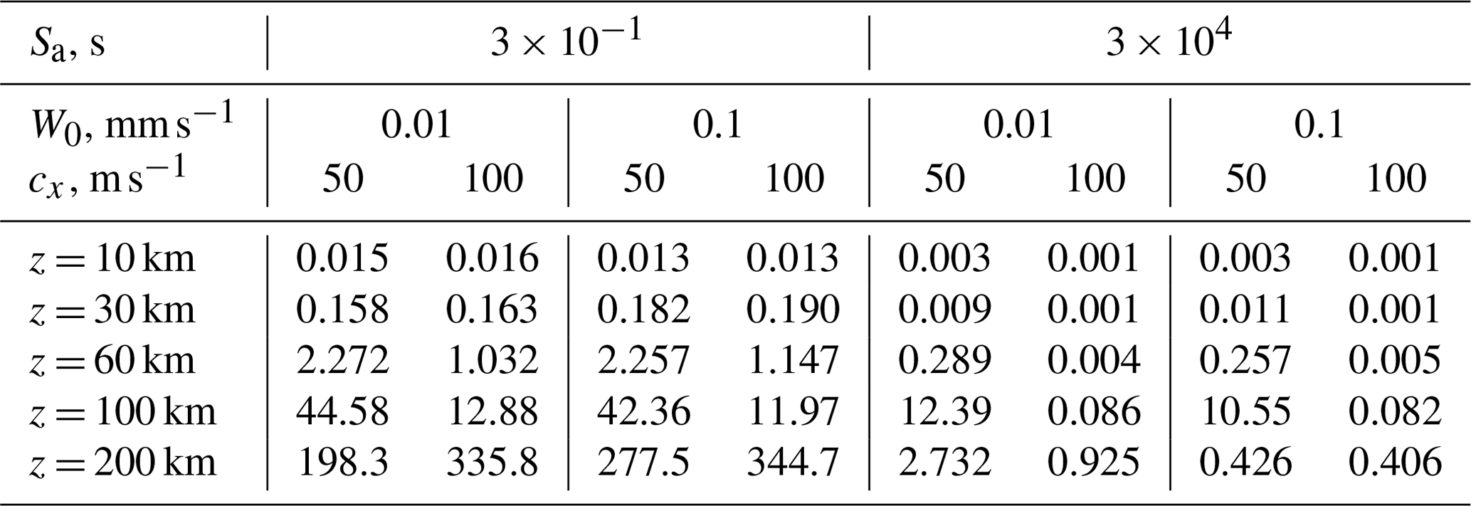
Relative contributions of residual and secondary AGWs can be estimated by the ratio $\mathit{\delta }w/W_{\mathrm{0}}$ at the beginning of the exponential tails in Figs. 2 and 3 at t = 170 h, which is presented in Table 2. For the steep wave source activation and deactivation at $s_{\mathrm{a}}=s_{\mathrm{d}}\approx$ 9 h in Eq. (7) and W₀ = 0.01 mm s⁻¹ in Eq. (5), Table 2 shows smaller ratios of the residual wave noise at altitudes below 200 km for the wave forcing with c_x = 100 m s⁻¹ compared to c_x = 50 m s⁻¹. At the sharp wave source activation and deactivation at $s_{\mathrm{a}}=s_{\mathrm{d}}\approx$ 0.3 s in Eq. (7), the ratios of residual waves are larger at all altitudes compared to the steep case in Table 2. For the wave forcing (Eq. 5) with c_x = 100 m s⁻¹, the ratios are comparable or smaller at altitudes below 150 km and larger above 150 km compared to the case of c_x = 50 m s⁻¹. Larger ratios of residual and secondary waves at sharp wave source triggering in Table 2 may explain generally larger AGW decay times τ₀ in the left columns of Table 1 for W₀ = 0.01 mm s⁻¹ in that the dissipation of stronger wave noise may require longer time intervals.

3.3 Larger-amplitude wave sources

The simulations described above were made for small-amplitude wave sources (Eq. 5) with W₀ = 0.01 mm s⁻¹. For larger W₀ = 0.1 mm s⁻¹, Fig. 4 reveals time variations in the vertical velocity standard deviations δw at different altitudes for c_x = 100 m s⁻¹ at the steep wave source activation and deactivation with $s_{\mathrm{a}}=s_{\mathrm{d}}\approx$ 9 h in Eq. (7), which is similar to Fig. 2.

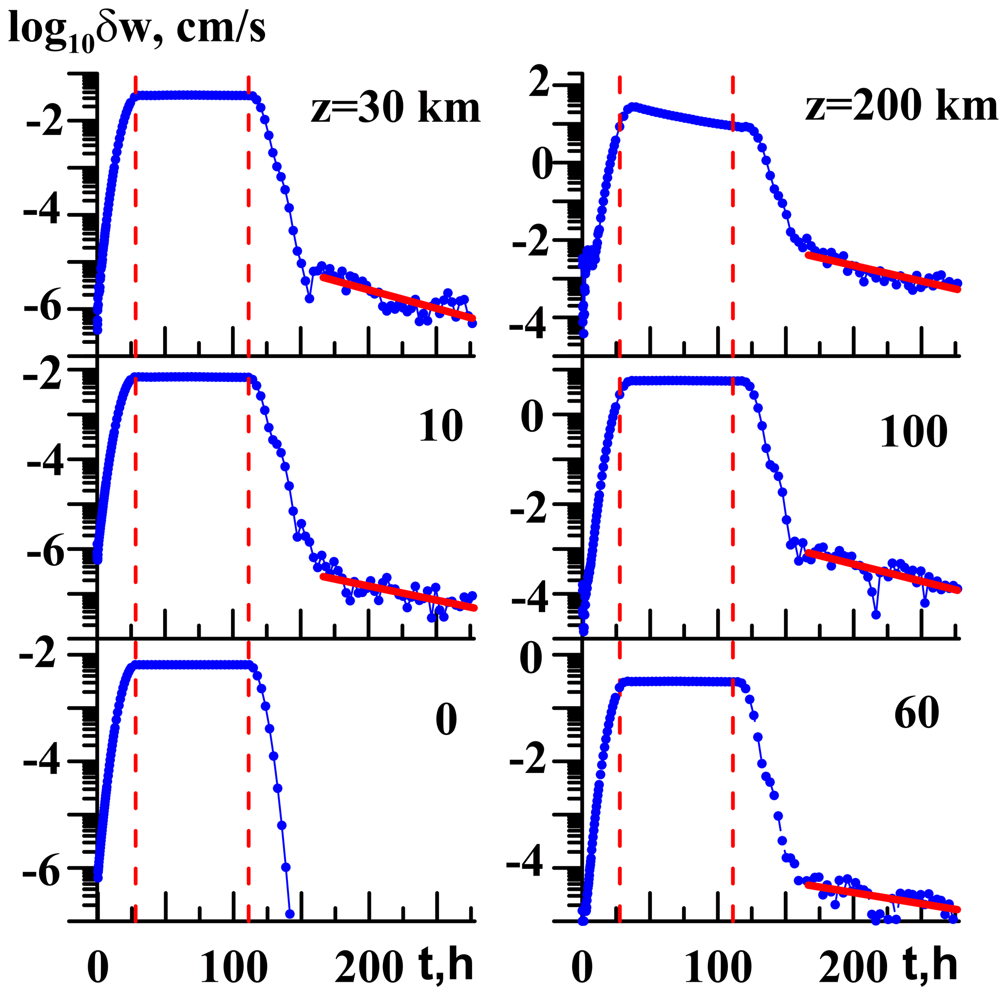
Figure 4 Same as Fig. 2, but for the surface wave source (Eq. 5) at c_x = 100 m s⁻¹ and W₀ = 0.1 mm s⁻¹.

Below an altitude of 100 km, one can see the intervals of quasi-constant AGW amplitudes after the end of the wave source activation at t=t_a (vertical dashed lines in Fig. 4). The theoretical time delay t_e between the wave source activation and the beginning of the steady-state AGW regime is 4 times smaller for c_x = 100 km than that for c_x = 50 km, as one can see comparing Figs. 2 and 4. After deactivations of the surface wave source (Eq. 5) at t=t_d, values of δw in Fig. 4 are first decreasing relatively fast due to the discontinuing generation of primary AGW modes at the lower boundary. At t > 150–170 h, slower decays of residual and secondary wave modes occur at all altitudes in Fig. 4 with decay times τ₀ listed in Table 1 for the steep and sharp wave source activation and deactivation.

Peculiarities of Fig. 4 for large W₀ are gradual decreases in AGW amplitudes during the wave source operation between moments t_a and t_d at high altitudes (see the top right panel of Fig. 4) in comparison with steady amplitudes in the respective panels of Fig. 2 for smaller W₀. The reason could be strong generations of wave-induced jet streams by large-amplitude AGWs at high altitudes. Figure 5 shows time variations in horizontal velocity u₀ averaged over a period of the surface wave source (Eq. 5) with W₀ = 0.1 mm s⁻¹ at different altitudes.

Figure 5 Time variations in the wave-induced mean horizontal velocity at different altitudes (marked with numbers) for the steep activations and deactivations of the surface wave source (Eq. 5) at c_x = 100 m s⁻¹ and W₀ = 0.1 mm s⁻¹. Dashed lines correspond to t=t_a and t=t_d in (Eq. 7).

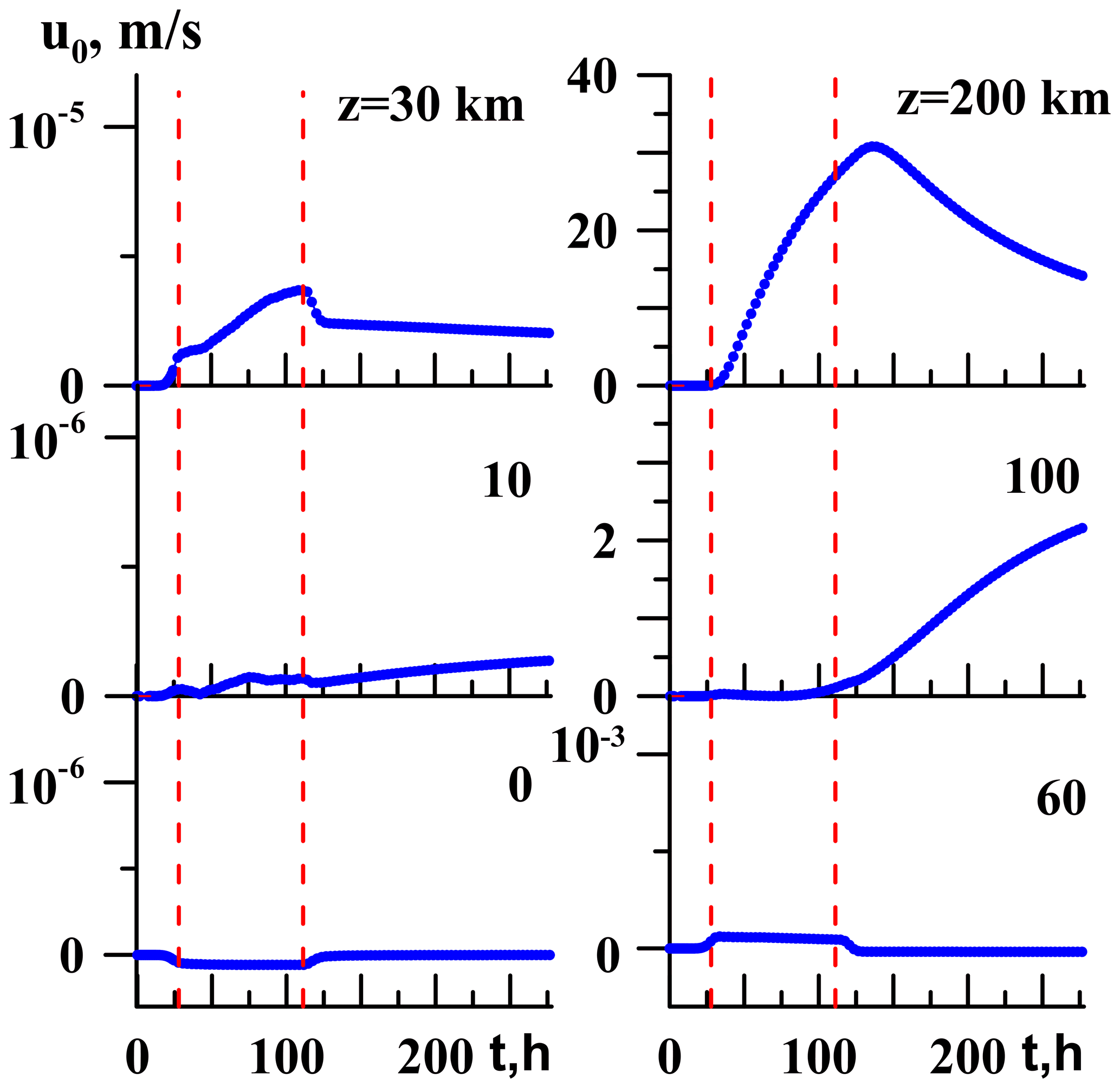
Generation of the wave-induced jet streams was simulated and considered in more detail in our previous papers (Gavrilov and Kshevetskii, 2015; Gavrilov et al., 2018). Larsen (2000) and Larsen et al. (2005) found frequent high horizontal wind velocities at altitudes near 100 km, which could be related to the wave-induced jet streams. In Fig. 5 for the strong wave excitation with amplitude of W₀ = 0.1 mm s⁻¹, one can see substantial u₀ rises at altitudes above 100 km during the wave source operation. Rising u₀ decreases the AGW intrinsic frequency and vertical wavelength (e.g., Gossard and Hooke, 1975). This may increase wave dissipation due to molecular viscosity and heat conductivity, leading to the gradual decrease in AGW amplitude in the top right panel of Fig. 4 in the time interval between t_a and t_d. The rate of u₀ weakening after the wave source deactivation decreases slowly in time in the top right panel of Fig. 5 so that the wave-induced horizontal winds are still substantial after hundreds of wave source periods at high altitudes. An interesting feature is an increase in u₀ at t > t_d in the panel of Fig. 5 for z = 100 km. This shows that residual and secondary AGWs slowly traveling upwards from below can produce substantial wave accelerations of the mean flow for a long time after deactivations of the surface wave sources.

Table 2 represents the ratio $\mathit{\delta }w/W_{\mathrm{0}}$ at the moment t≈ 170 h for larger-amplitude surface wave sources (Eq. 5), which may characterize a proportion of residual and secondary waves after the fast-traveling modes of the wave excitation disappear. At steep wave source activations and deactivations with $s_{\mathrm{a}}=s_{\mathrm{d}}\approx$ 9 h, Table 2 demonstrates approximately the same $\mathit{\delta }w/W_{\mathrm{0}}$ values below an altitude of 100 km and generally smaller values at higher altitudes for W₀ = 0.1 mm s⁻¹ as compared with W₀ = 0.01 mm s⁻¹ if one considers columns for fixed c_x at different W₀ values. This may be caused by the transfer of wave energy to wave-induced jets discussed above, which can also provide larger reflections and dissipation of wave components with larger amplitudes.

AGW decay times in Table 1 for W₀ = 0.1 mm s⁻¹ at altitudes below 100 km are generally larger for the sharp wave source triggering (s_a = s_d≈ 0.3 s) than those for the steep triggering ($s_{\mathrm{a}}=s_{\mathrm{d}}\approx$ 9 h), similar to the case of smaller wave source amplitude discussed in Sect. 3.2. At high altitudes in Table 1 for W₀ = 0.1 mm s⁻¹, wave decay times for the sharp wave source deactivation become smaller than those for the steep triggering.

3.4 Spatial structure of AGW fields

To analyze changes in the spatial structure of simulated AGW fields, Figs. 6 and 7 present cross-sections of the field of wave vertical velocity by the XOZ vertical plane at different time moments during activations and deactivations of the surface wave sources (Eq. 5) with the steep values of $s_{\mathrm{a}}=s_{\mathrm{d}}\approx$ 9 h in Eq. (7). Figure 6a shows that after dispersion and dissipation of the initial AGW pulse just after the wave forcing activation time, t_a≈ 28 h, wave fronts become inclined to the horizon. This behavior is characteristic for the main IGW mode with the period τ ∼ 4.7 h, which dominates in the spectrum of the wave source with c_x = 50 m s⁻¹, similar to Fig. 1a. In the middle and at the end of quasi-stationary intervals shown in Figs. 2–4, the inclined wave fronts in Fig. 6b and c expand to the entire atmospheric region considered, and wave amplitudes become larger compared to Fig. 6a.

Figure 6 AGW vertical velocity fields at times t≈ 30 h (a), t≈ 70 h (b) and t≈ 110 h (c) for the steep rate of activating and deactivating the wave source (Eq. 5) with c_x = 50 m s⁻¹ and W₀ = 0.01 mm s⁻¹.

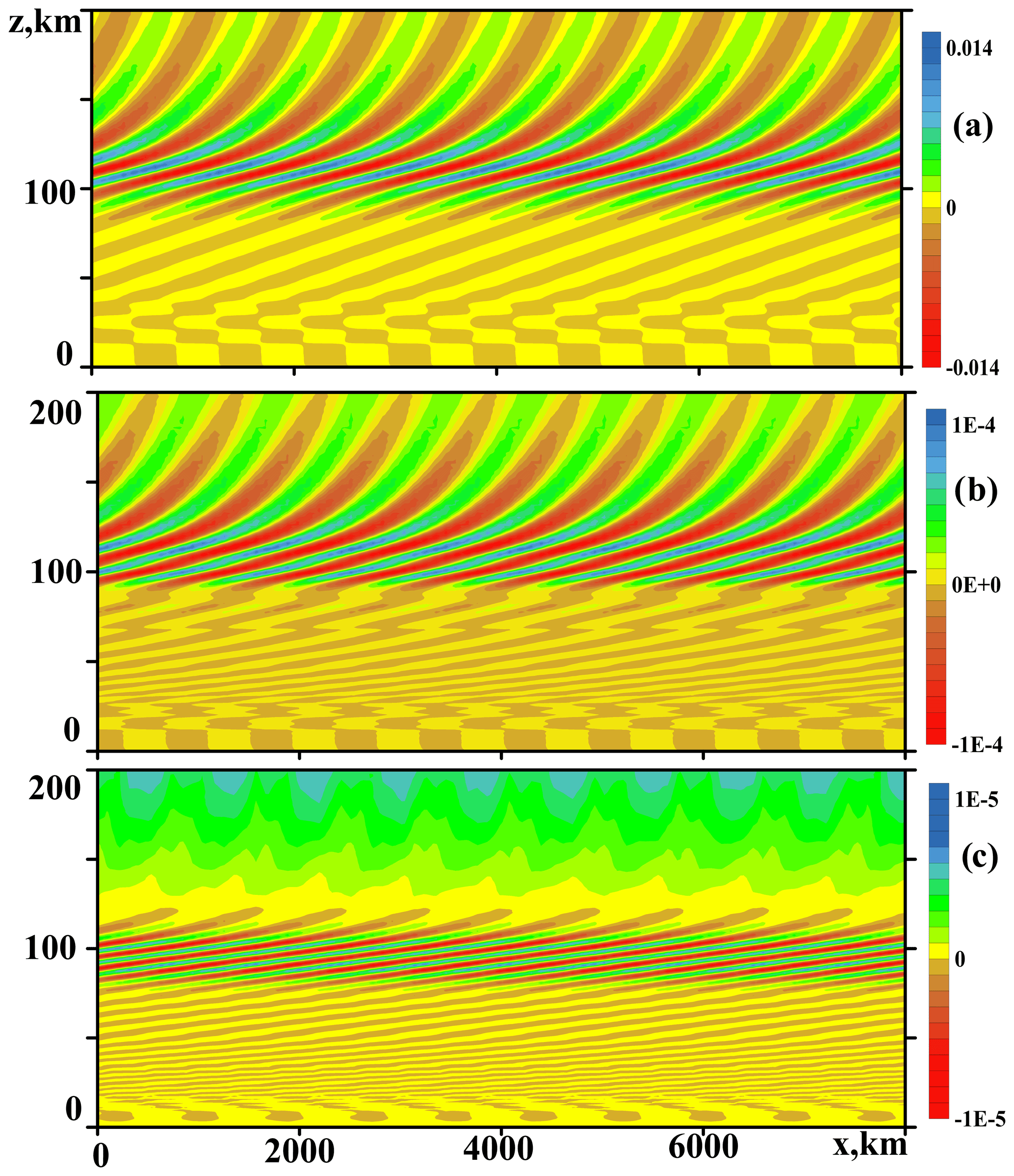
Figure 7 Same as Fig. 6, but for time moments after the wave source steep deactivating: t≈ 140 h (a), t≈ 200 h (b) and t≈ 250 h (c).

Cross-sections shown in Fig. 7 correspond to time moments after the wave source (Eq. 5) deactivation at t_d≈ 110 h. Figure 7a shows that just after turning off the wave source, the inclined fronts are destroyed first in the lower atmosphere. Above 50 km altitude, the wave field structure in Fig. 7a is still similar to Fig. 6b and c. Later, in Fig. 7b and c, wave amplitudes become smaller, especially at low and high altitudes. Therefore, maximum AGW amplitudes in Fig. 7c are located at altitudes 80–120 km. This explains the growing wave-induced horizontal velocity at 100 km altitude after the wave source deactivation in the respective panel of Fig. 5. At heights below 50 km in Fig. 7, directions of wave front inclinations to the horizon are opposite to those in Fig. 6. This reveals the existence of downward-traveling IGW modes in the stratosphere and troposphere after deactivations of the surface wave sources. Such modes could be produced by partial reflections of primary upward-traveling IGWs at higher atmospheric levels (see Sect. 4).

Figure 7b and c show increasing numbers of small-scale structures, which can be formed by slow short-wave residual wave modes, which appear due to broad wave source spectra in Fig. 1 and due to the generation of secondary waves by nonlinear interactions of primary AGW modes.

4 Discussion

The timescale of AGW dissipation in the turbulent atmosphere can be estimated as follows (Gossard and Hooke, 1975):

$$\begin{array}{}\text{(8)}& {\mathit{\tau }}_{\mathrm{d}}={\mathit{\lambda }}_z^{\mathrm{2}}/\mathrm{2}\mathit{\pi }{K}_{\mathrm{z}},\end{array}$$

where K_z is the total vertical coefficient of turbulent and molecular viscosity and heat conductivity. For the main primary AGW modes simulated in this study and with λ_z ∼ 15–30 km (see Sect. 3.1), τ_d ∼ 10³–10⁵ h at altitudes below 100 km. These values are much larger than the AGW decay times τ₀ in Table 1. Therefore, attenuations of primary AGW modes in the middle atmosphere shown in Figs. 2–7 after deactivations of the surface wave forcing cannot be explained by direct turbulent and molecular dissipations.

AGWs propagating in the atmosphere with vertical gradients of the background fields are subject to partial reflections. In particular, strong wave reflections occur at altitudes of 110–150 km, where large vertical gradients of the mean temperature exist (e.g., Yiğit and Medvedev, 2010; Walterscheid and Hickey, 2011; Gavrilov and Kshevetskii, 2018). Partial reflections of wave energy propagating upwards from the wave sources before their deactivations may produce vertically standing waves in the middle atmosphere. Simulations by Gavrilov and Yudin (1987) showed that the standing-wave ratio for IGW amplitudes might reach 0.4 at altitudes below 100 km. After deactivations of wave sources, vertically traveling AGW modes propagate quickly upwards and dissipate at higher atmospheric altitudes. This gives fast decreases in AGW amplitudes at all heights in Figs. 2 and 4 just after the wave source deactivations. After disappearing fast-traveling modes, residual quasi-standing AGWs produced by partial reflections may form long-lived wave structures in the atmosphere shown in Figs. 2–7.

The standing AGWs discussed above are composed of the primary wave modes traveling upwards from the surface wave sources (Eq. 5) and downward-propagating waves reflected at higher atmospheric levels. After the wave source deactivations, the reflected downward waves propagate to the Earth's surface and create wave fronts at low altitudes in Fig. 7, which are inclined to the horizon in directions opposite to the fronts of primary AGWs shown in Fig. 6. For the used smooth climatological temperature profiles from the NRLMSISE-00 model (see Fig. 1 of the paper by Gavrilov et al., 2018) AGW reflections inside the troposphere are smaller than the reflection from the ground caused by lower boundary conditions given by Eq. (4). Therefore, the abovementioned downward-traveling waves are reflected from the ground and propagate upwards back to the middle atmosphere. Kurdyaeva et al. (2018) showed that such AGW reflections from the ground could be equivalent to additional wave forcing at the lower boundary, which is still effective after deactivations of primary surface wave sources. Waves traveling upward from the ground and reflected again at higher altitudes can maintain quasi-standing AGW structures for a long time (see Fig. 7). As long as wave reflections are partial, portions of wave energy can propagate to higher altitudes and dissipate there for a long time. This can explain the relatively large AGW decay times τ₀ in the lower and middle atmosphere shown in Figs. 2–4 and in Table 1. Even after substantial time from the wave source turning off, AGW structures in Fig. 7b and c at altitudes above 50 km are still similar to those shown in Fig. 6 during active wave forcing.

The panels of Fig. 2 for the steep wave source activation and deactivation demonstrate periodical increases and decreases in the residual wave noise standard deviations (especially at low altitudes), which are superimposed on the exponential decay at t>t_d. This may be caused by long-term biases between upward and downward wave packages reflected from the ground and from the upper atmosphere, which propagate through the middle atmosphere. Increased molecular and turbulent AGW dissipation makes periodical amplitude variations less noticeable in the panels of Fig. 2 for high altitudes. These biases are also less noticeable in the respective panels of Fig. 3 for the sharp wave source activation because the wave source spectra in Fig. 1 are smoother and wider in this case compared to the smooth deactivation of the wave excitation.

One can raise the question as to the extent to which the results shown in Tables 1 and 2 may depend on so-called “numerical viscosity” caused by mathematical algorithms used in the model. Our model is based on special numerical algorithms accounting for the main conservation laws (Gavrilov and Kshevetskii, 2013, 2014). Therefore, the numerical viscosity is very small. Test simulations showed that in the absence of physical dissipation, wave modes might exist in the model for hundreds of wave periods without noticeable decreases in their amplitudes. In addition, simulated ratios of standard deviations of different components of long-wave fields in the middle atmosphere follow to the polarization relations of conventional theory of nondissipative AGWs (Gavrilov et al., 2015). Therefore, we assume that in the present model, the numerical viscosity is much smaller than molecular and turbulent viscosity and heat conduction, which are involved in the model at all altitudes.

The ratios $\mathit{\delta }w/W_{\mathrm{0}}$ at t≈ 170 km shown in Table 2 may reflect proportions of the residual and secondary AGW modes in the beginning of quasi-exponential fits in Figs. 2–4. For the steep wave forcing activations and deactivations, in the right part of Table 2, one can see larger ratios for wave modes with c_x = 50 m s⁻¹ at all altitudes. This corresponds to longer intervals of fast decreases in AGW amplitudes after deactivations of the wave sources in Fig. 4 compared to Fig. 2. Considerations of the respective right columns of Table 1 reveal larger decay times τ₀ of waves with c_x = 100 m s⁻¹ due to their larger vertical wavelength and smaller dissipation in the middle atmosphere.

Comparisons of the right columns in Table 2 with the same c_x and different W₀ show that values of $\mathit{\delta }w/W_{\mathrm{0}}$ for each c_x are approximately equal at altitudes below 60 km and become smaller at higher altitudes for larger-amplitude wave sources. This may reflect larger transfers of AGW energy to wave-induced jet streams and to secondary nonlinear modes produced by larger-amplitude waves. The respective right columns of Table 1 show higher decay times τ₀ of larger-amplitude wave noise corresponding to W₀ = 0.1 mm s⁻¹ at altitudes higher than 100 km. This noise can be maintained for a long time by wave energy fluxes propagating with stronger residual and secondary waves from the middle atmosphere to higher altitudes.

For the sharp activations and deactivations of the wave sources (Eq. 5), the left columns of Table 2 show values of $\mathit{\delta }w/W_{\mathrm{0}}$ which are much larger compared to the respective right columns for the steep wave forcing triggering. These ratios are less dependent on the speed and amplitude of simulated AGWs and could be connected with wave pulses produced by sharp activations and deactivations of the wave sources (see spectra in Fig. 1). AGW decay times for the sharp triggering in the respective left columns of Table 1 are also less dependent on wave parameters.

Substantial numbers of small-scale structures in Fig. 7b and c show increased proportions of wave modes, produced due to high-frequency tails of the wave forcing spectra in Fig. 1, also due to multiple reflections and nonlinear interactions of these modes. Nonlinear AGW interactions and generations of secondary waves should be stronger at high altitudes due to increased wave amplitudes (Vadas and Liu, 2013; Gavrilov at al., 2015). Then the secondary waves can propagate downwards and make small-scale wave perturbations at all atmospheric altitudes (see Figs. 6 and 7). The AGW decay times τ₀ in Table 1 are generally larger for longer AGW modes with c_x = 100 m s⁻¹. This may be explained by their smaller dissipation due to turbulent and molecular viscosity and heat conductivity in the atmosphere. Due to small coefficients of turbulent dissipation in the stratosphere and mesosphere, maximum AGW decay times in Table 1 exist at altitudes of 30–100 km. Quasi-standing and secondary AGWs may exist there for several days after deactivations of the wave forcing. Wave energy can slowly penetrate upwards from the stratosphere and mesosphere and maintain a background level of AGW activity at higher altitudes. Figure 7c reveals that after 10 d of simulations, the largest amplitudes of the residual wave field exist at altitudes of 70–110 km. This is enough for the creation of wave accelerations, which can act and modify the mean velocity at altitudes near 100 km for a long time after the wave source deactivations (see respective panels of Fig. 5).

Simulations presented in this paper are made for horizontally uniform wave excitation at the ground described by Eq. (5). At the same time, many wave sources are localized in different atmospheric regions. Our test simulations for localized wave sources (e.g., Kurdyaeva et al., 2018) showed that near an isolated deactivated wave source the amplitude decay could be faster due to horizontal dispersion of wave packets. However, at low altitudes these wave packets can go around the globe and return to the initial point similar to wave packages observed after big explosions of meteorites and volcanoes (e.g., Ewing and Press, 1955; Roberts et al., 1982). Therefore, globally, wave packets may exist in the atmosphere for a long time. For several local wave sources, wave packets from different sources may overlap and produce more horizontally uniform long-lived wave noise. Therefore, the horizontally inhomogeneous model considered in this paper may reflect general global features of AGW decay processes in the atmosphere. Isolated and multiple local wave sources require special considerations in subsequent papers.

The simulations described above were made for single relatively long AGW spectral components which experience little dissipation in the stratosphere and mesosphere. Real wave fields in the atmosphere are superpositions of a wide range of spectral components generated by a variety of different wave sources. However, after deactivations of wave sources, fast-traveling spectral components disperse to higher altitudes, and short-wave modes are strongly dissipated due to turbulent and molecular viscosity and heat conductivity. Therefore, one may expect that at the final stage of wave disappearance after deactivations of wave forcing, wave fields in the stratosphere and mesosphere should consist of vertically standing, relatively long spectral components, similar to those considered in the present study. These wave fields may contain substantial proportions of residual and secondary wave modes produced by multiple reflections and nonlinear interactions. Such an impression is probably true for the residual wave noise, which may exist for a long time after the wave source deactivation. However, amplitudes of this residual noise become smaller in time, and near active wave sources, amplitudes of generated primary AGWs may far exceed the wave noise.

In this paper, we analyze idealistic cases of long-lived horizontally homogeneous coherent wave sources producing quasi-stationary wave fields in the atmosphere. Such modeling is useful for comparisons of simulated results with standard AGW theories. However, many AGW sources in the atmosphere are local and operate for a short time, which is not enough for developments of steady-state wave fields. Further simulations are required for studying wave decay processes after deactivating such local short-lived wave sources in the atmosphere.

5 Conclusion

In this study, the high-resolution numerical model AtmoSym is applied for simulating non-stationary, nonlinear AGWs propagating from surface wave sources to higher atmospheric altitudes. After activating the surface wave forcing and fading away initial wave pulses, AGW amplitudes reach a quasi-stationary state. Then the surface wave forcing is deactivated in the numerical model, and amplitudes of primary traveling AGW modes quickly decrease at all altitudes due to discontinuation of wave energy generation by the surface wave sources. However, later the standard deviation of the residual and secondary wave perturbations produced by slow components of the wave source spectrum, multiple reflections and nonlinear interactions experiences slower exponential decreases. The decay time of the residual AGW noise may vary between 20 and 100 h, with maxima in the stratosphere and mesosphere. Standard deviations of the residual AGWs in the atmosphere are much larger at sharp activations and deactivations of the wave forcing compared to the steep processes. These results show that transient wave sources in the lower atmosphere could create long-lived residual and secondary wave perturbations in the middle atmosphere, which can slowly propagate to higher altitudes and form a background level of wave noise for time intervals of several days after deactivations of wave sources. Such behavior should be taken into account in parameterizations of AGW impacts in numerical models of dynamics and energy of the middle atmosphere.