Interactive biogenic emissions and drought stress effects on atmospheric composition in NASA GISS ModelE

Drought is a hydroclimatic extreme that causes perturbations to the terrestrial biosphere and acts as a stressor on vegetation, affecting emissions patterns. During severe drought, isoprene emissions are reduced. In this paper, we focus on capturing this reduction signal by implementing a new percentile isoprene drought stress (y_d) algorithm in NASA GISS ModelE based on the MEGAN3 (Model of Emissions of Gases and Aerosols from Nature Version 3) approach as a function of a photosynthetic parameter (V_c,max) and water stress (β). Four global transient simulations from 2003–2013 are used to demonstrate the effect without y_d (Default_ModelE) and with online y_d (DroughtStress_ModelE). DroughtStress_ModelE is evaluated against the observed isoprene measurements at the Missouri Ozarks AmeriFlux (MOFLUX) site during the 2012 severe drought where improvements in the correlation coefficient indicate it is a suitable drought stress parameterization to capture the reduction signal during severe drought. The application of y_d globally leads to a decadal average reduction of ∼2.7 %, which is equivalent to ∼14.6 Tg yr⁻¹ of isoprene. The changes have larger impacts in regions such as the southeastern US. DroughtStress_ModelE is validated using the satellite ΩHCHO column from the Ozone Monitoring Instrument (OMI) and surface O₃ observations across regions of the US to examine the effect of drought on atmospheric composition. It was found that the inclusion of isoprene drought stress reduced the overestimation of ΩHCHO in Default_ModelE during the 2007 and 2011 southeastern US droughts and led to improvements in simulated O₃ during drought periods. We conclude that isoprene drought stress should be tuned on a model-by-model basis because the variables used in the parameterization responses are relative to the land surface model hydrology scheme (LSM) and the effects of y_d application could be larger than seen here due to ModelE not having large biases of isoprene during severe drought.

1 Introduction

In present-day conditions terrestrial ecosystems release about 1000 Tg C yr⁻¹ of biogenic volatile organic compounds (BVOCs) into the atmosphere, and there is an additional smaller emission from marine ecosystems (Guenther et al., 2012). The majority of BVOCs emitted from vegetation are isoprene and monoterpenes (Guenther et al., 2006, 2012). Representing over half of emitted BVOCs, isoprene is the dominant species globally with reported ranges of 440–600 Tg C yr⁻¹ (Guenther et al., 2012) and high emission factors from some, but not all, broadleaf trees including species of oak, willow, palm oil, and eucalyptus (Benjamin et al., 1996; Geron et al., 2000). Isoprene is produced from carbon substrates generated during photosynthesis and contributes to abiotic stress tolerance from water and temperature stress (Loreto and Sharkey, 1990; Monson et al., 2021). Isoprene emissions peak during warm, sunnier months of the growing season (March–October) (Opacka et al., 2021). Isoprene has a chemical lifetime of approximately 1 h via oxidation by the hydroxyl radical (OH), producing organic aerosols and oxidation products that contribute to ozone (O₃) formation (Carlton et al., 2009). Biogenic isoprene emissions affect atmospheric composition and climate and in turn depend on environmental factors including light, temperature, photosynthetically active radiation (PAR), leaf area index (LAI), water stress, ambient O₃, and CO₂ concentrations. Thus, the response of isoprene emissions to weather extremes and changing climates is highly uncertain.

Drought is a common abiotic stress to terrestrial ecosystems characterized by low soil moisture, usually associated with high temperature and low precipitation. However, even boreal forests undergo winter drought due to frozen soils. Recent work has shown a strong correlation between drought severity and fine-mode aerosols in the US and estimated that regions undergoing severe drought see up to 17 % surface enhancement of aerosols during the growing season (Wang et al., 2017). This suggests a strong perturbation of drought to atmospheric aerosols, likely caused by changing BVOC emissions due to drought stress. Limited field and lab measurements have shown that during drought, isoprene has a unique emission response whereby an initial increase in temperature causes an increase in emission, but prolonged or severe drought causes a decrease in emissions due to the shutdown of physiological processes (Potosnak et al., 2014). This behavior is not reproduced by commonly used BVOC emission models such as the Model of Emissions of Gases and Aerosols from Nature Version 2.1 (MEGAN2.1), which has a simple drought algorithm that is often not used due to the unavailability of the required driving variables in chemistry climate models (CCMs), and the Biogenic Emission Inventory System (BEIS), which does not include a drought algorithm as an option.

Isoprene flux observations at the Missouri Ozarks (MOFLUX) AmeriFlux site in Missouri (Fig. S1 in the Supplement) recorded a moderate drought in summer 2011 (Potosnak et al., 2014) and a particularly severe drought event in summer 2012 (Seco et al., 2015). To the best of our knowledge, these are the only in situ isoprene flux measurements capturing a drought anywhere. Using the MOFLUX observations, Jiang et al. (2018) developed an isoprene drought stress activity factor for MEGAN3 (Model of Emissions of Gases and Aerosols from Nature Version 3) designed to reduce emissions of isoprene during drought. The previous MEGAN2.1 isoprene drought parameterization utilized soil moisture and the soil wilting point threshold to include impacts of drought on photosynthetic processes. The MEGAN3 isoprene drought stress activity factor is a more process-based parameterization based on a photosynthetic parameter (V_c,max) and water stress (β) from the Community Land Model (CLM) as coupled with the CAM-Chem climate model (Jiang et al.,  2018). V_c,max is the maximum carboxylation capacity of a leaf (usually in units of micromoles of CO₂ per leaf area per time); that is, it is the ability of a plant to convert CO₂ into sugar and hence determine productivity of carbon substrates for biogenic volatile organic compound (BVOC) production when no other conditions are limiting. β is a scaling factor between zero and 1 used in CLM to reduce V_c,max due to plant water stress. MEGAN3 isoprene drought stress was also incorporated into the CSIRO chemical transport model (C-CTM) with the Australian land surface model Mk3.6 Global Climate Model and the Soil-Litter-Iso model with a focus on Australia (Emmerson et al., 2019). Both prior modeling studies (Jiang et al., 2018; Emmerson et al., 2019) only looked at the drought effects on O₃; here we study the combined effect of drought on O₃ and the formaldehyde column.

The accurate simulation of stress-affected emissions of isoprene during extreme hydroclimate events (i.e., drought) is crucial to understanding vegetation–climate–chemistry feedbacks because isoprene is a precursor to tropospheric O₃ and secondary organic aerosol (SOA), both being climate forcers as well as air pollutants. Here we focus on deriving a model-specific tuned isoprene drought stress factor that is coupled into the existing MEGAN2.1 framework in NASA GISS ModelE, an Earth system model, to model the effect of drought on isoprene emissions and their effect on atmospheric composition. The model-specific tuning is required due to different land system models parameterizing key variables of V_c,max and β in different ways with varying distributions. The model's drought effects were extensively evaluated across the US due to the availability of observational evidence during drought at the MOFLUX site and due to the EPA monitoring network for O₃ and PM_2.5 (particulate matter ≤2.5 µm) (Wang et al., 2017). While the MOFLUX data are the only available measurements of isoprene emissions during drought, formaldehyde (HCHO), the high-yield oxidation product of isoprene, can be used as a proxy for isoprene emissions when no direct ground-based observations of isoprene are available (Zhu et al., 2016). Section 2 describes the modeling approaches used to represent drought impacts on isoprene emissions. Section 3 describes the comparison of modeled isoprene emissions to observations at the MOFLUX site during drought along with the necessity of building a model-specific isoprene drought stress parameterization. Section 4 details the comparisons between simulations with model-specific tuned isoprene drought stress (DroughtStress_ModelE) and observational O₃, PM_2.5, and tropospheric formaldehyde columns (ΩHCHO) over North America.

2 Methods and data

2.1 The biogenic emission model MEGAN

MEGAN is a widely used BVOC emissions model that is implemented in many CCMs. Here we briefly describe MEGAN2.1 as implemented in ModelE. MEGAN2.1 calculates the net primary emissions for 20 compound classes, which are speciated into over 150 species such as isoprene and monoterpenes (Guenther et al., 2012). The emission rate (µg per grid cell per hour) of each compound into the above-canopy atmosphere from a model grid cell is calculated as

$$\begin{array}{}\text{(1)}& \text{emission}=\text{EF}\times y\times S,\end{array}$$

where EF ($\mathrm{\mu }\mathrm{g}{\mathrm{m}}^{-\mathrm{2}}{\mathrm{h}}^{-\mathrm{1}}$) is emission factor per compound, y is the dimensionless emission activity factor that accounts for emission response to phenological and meteorological conditions, and S is the grid cell area (m²).

The emission activity factor y for each compound is calculated following the MEGAN2.1 parameterization (Guenther et al., 2006, 2012; Henrot et al., 2017):

$$\begin{array}{}\text{(2)}& y=y_{\mathrm{CE}}\times y_{\mathrm{A}}\times y_{\mathrm{d}}\times y_{{\mathrm{CO}}_{\mathrm{2}}},\end{array}$$

where y_CE is the canopy environment coefficient (assigned a value of 1 for standard conditions) that takes into account variations associated with LAI (m² m⁻²), photosynthetic photon flux density (PPFD) (µmol of photons in the 400–700 nm range per meter squared per second – m⁻² s⁻¹), and temperature (K). y_A is the leaf age emission activity factor, the parameterization of which is based on coefficients of the decomposition of the canopy into new, growing, mature, and senescing leaves for current and previous months' LAI (Guenther et al., 2006, 2012). y_d is the isoprene drought stress activity factor, and $y_{{\mathrm{CO}}_{\mathrm{2}}}$ is the isoprene emission activity factor associated with CO₂ inhibition (for all other compounds y_d and $y_{{\mathrm{CO}}_{\mathrm{2}}}=\mathrm{1}$) (Heald et al., 2009). The biogenic emission module implemented in ModelE follows the ECHAM6-HAMMOZ online MEGAN2.1 implementation (Henrot et al., 2017) in a CCM. Within ModelE the MEGAN2.1 module maps the 16 plant functional types (PFTs) from Ent TBM (Terrestrial Biosphere Model) (Kim et al., 2015) into 16 MEGAN PFTs and contains 13 chemical compound classes. ModelE uses a modified MEGAN2.1 following Henrot et al. (2017) to provide a framework to simulate isoprene emissions and uses prescribed emissions factors per PFT to simulate emissions per compound class.

In Henrot et al. (2017), to avoid using a detailed canopy environment model calculating light and temperature at each canopy depth, the parameterized canopy environmental emission activity (PCEEA) approach from Guenther et al. (2006) is used to replace y_CE with a parameterized canopy environment activity factor ($y_{\mathrm{LAI}}\times y_{\mathrm{P}}\times y_{\mathrm{T}}$). With this approach the light-dependent and light-independent factors are multiplied by y_LAI not LAI, so they are not directly proportional to LAI. This approach allows for calculation of light-dependent emissions following isoprene emission response to temperature; it is assumed that the light-dependent factor (LDF) equals 1 for isoprene and light-independent emissions follow the monoterpene exponential temperature response. Please see Guenther et al. (2006, 2012) and Henrot et al. (2017) for activity factor parameterizations. At any given time step in ModelE, the emissions formula for a compound class (c) and PFT (i) (units kg m⁻² s⁻¹) is given by

$$\begin{array}{}\text{(3)}& \begin{array}{rl}{\text{emission}}_{i,\mathrm{c}}=& \left(\mathrm{1}\times {\mathrm{10}}^{-\mathrm{9}}/\mathrm{3600}\right)\times \left({\text{EF}}_{i,\mathrm{c}}\times {\text{PFTboxf}}_i\right)\\ & \times y_{\mathrm{LAI}}\times y_{\mathrm{A}}\times y_{\mathrm{d}}\times y_{{\mathrm{CO}}_{\mathrm{2}}}\\ & \times (\left(\mathrm{1}-\text{LDF}\right)\times y_{\mathrm{TLI}}+\text{LDF}\times y_{\mathrm{P}}\times y_{\mathrm{TLD}})\\ & \times {\text{SF}}_{\mathrm{c}}\times {\text{MWC}}_{\mathrm{c}},\end{array}\end{array}$$

where EF_i,c is the emissions factor ($\mathrm{\mu }\mathrm{g}{\mathrm{m}}^{-\mathrm{2}}{\mathrm{h}}^{-\mathrm{1}}$) for a given PFT and compound class, PFTboxf_i is the fraction of the grid cell (ranging from zero to 1) covered by PFT_i, and SF_c is a linear scale factor for compound class c. The activity factors, y, listed in Eq. (3) are unitless and account for the emissions response to leaf area index (LAI), aging (A), drought (d), CO₂ (CO₂), and PPFD (P). The LDF weights the contributions from light-independent (y_TLI) and light-dependent (y_TLD) emissions response to temperature. MWC_c stands for a molecular weight conversion to remove non-carbon mass, if appropriate ($\mathrm{1}\times {\mathrm{10}}^{-\mathrm{9}}/\mathrm{3600}$: the numerator converts units from $\mathrm{\mu }\mathrm{g}{\mathrm{m}}^{-\mathrm{2}}{\mathrm{h}}^{-\mathrm{1}}$ to kg m² s⁻¹, and the denominator is the time step conversion for seconds in an hour). Note that although the drought activity factor y_d is present in ModelE, it is set to equal 1 in all cases prior to this work, meaning no drought effects on BVOC emissions in the model.

For example, the emission formula for the compound class of isoprene in ModelE for PFT_i is as follows (where LDF =1):

$$\begin{array}{}\text{(4)}& \begin{array}{rl}{\mathrm{\text{isoprene}}}_i=& \left(\mathrm{1}\times {\mathrm{10}}^{-\mathrm{9}}/\mathrm{3600}\right)\times \left({\text{EF}}_{i,\mathrm{isoprene}}\times {\text{PFTboxf}}_i\right)\\ & \times y_{\mathrm{LAI}}\times y_{\mathrm{A}}\times y_{\mathrm{d}}\times y_{{\mathrm{CO}}_{\mathrm{2}}}\times \left(y_{\mathrm{P}}\times y_{\mathrm{TLD}}\right)\\ & \times {\text{SF}}_{\mathrm{isoprene}}\times (\mathrm{60.05}/\mathrm{68.12})\end{array}\end{array}$$

2.2 MEGAN2.1 isoprene drought stress emission algorithm

Guenther et al. (2006) introduced isoprene drought stress as a soil-moisture-dependent algorithm called y_SM. This isoprene drought stress activity factor relied upon soil moisture and wilting point to apply drought stress to isoprene emissions. The algorithm for soil moisture isoprene drought stress is as follows:

$$\begin{array}{}\text{(5a)}& {\displaystyle }{y}_{\mathrm{SM}}=\mathrm{1}\text{when}\mathit{\theta }>{\mathit{\theta }}_{\mathrm{1}},\text{(5b)}& {\displaystyle }{y}_{\mathrm{SM}}={\displaystyle \frac{\mathit{\theta }-{\mathit{\theta }}_{\mathrm{w}}}{{\mathrm{\Delta }}_{{\mathit{\theta }}_{\mathrm{1}}}}}\text{when}{\mathit{\theta }}_{\mathrm{w}}<\mathit{\theta }<{\mathit{\theta }}_{\mathrm{1}},\text{(5c)}& {\displaystyle }{y}_{\mathrm{SM}}=\mathrm{0}\text{when}\mathit{\theta }<{\mathit{\theta }}_{\mathrm{w}},\end{array}$$

where θ is soil moisture (volumetric water content m³ m⁻³), θ_w is the point beyond which plants cannot extract water from soil that is known as the wilting point (units: m³ m⁻³), ${\mathrm{\Delta }}_{{\mathit{\theta }}_{\mathrm{1}}}$ (0.06 in Guenther et al., 2006 and 0.04 in Guenther et al., 2012) is an empirical parameter, and θ₁ is defined as ${\mathit{\theta }}_{\mathrm{w}}+{\mathrm{\Delta }}_{{\mathit{\theta }}_{\mathrm{1}}}$. Soil moisture and wilting point are not widely available parameters in models, and y_SM was not widely adopted to represent isoprene drought stress as studies showed substantial uncertainty associated with the soil-moisture-predicted response of isoprene emission to water stress and in the selection of wilting point values (Müller et al., 2008; Tawfik et al., 2012; Sindelarova et al., 2014; Huang et al., 2015; Jiang et al., 2018). There are also challenges associated with validating soil moisture datasets due to the limited spatial coverage of in situ root-zone measurements in the contiguous United States (Ochsner et al., 2013). A study found that the accurate simulation of soil moisture in land surface models was highly model-dependent due to the differing horizontal and vertical spatial resolution of such models at large scales (Koster et al., 2009). Potosnak et al. (2014) determined that the selection of different wilting point values greatly impacted the drought impacts on biogenic isoprene emission. With these associated challenges, it was rare to find isoprene drought stress implemented in CCMs, and thus a new isoprene drought activity factor needed to be developed that could be easily incorporated into a variety of models that had a land surface model (LSM) or terrestrial biosphere model (TBM).

2.3 MEGAN3 isoprene drought stress emission algorithm

Jiang et al. (2018) developed a new isoprene drought stress activity factor in MEGAN3 that focuses on photosynthetic carboxylation capacity and water stress to model reductions of vegetative isoprene during drought. Vegetation responds to high water stress by undergoing physiological, morphological, and biochemical changes (Seleiman et al., 2021). During high water stress plants experience leaf area reduction and loss of leaves, decreasing photosynthetic rate due to stomatal closure, decreasing stomatal conductance, transpiration, and evaporative cooling. During drought there is also decreasing Rubisco efficiency, which is the enzyme used for carbon fixation of atmospheric CO₂ into useable sugar molecules during photosynthesis (Seleiman et al., 2021). These are just a few of the ways vegetation responds to water stress, which impacts isoprene emissions. The algorithm was developed using isoprene flux observations during the severe drought of the summer of 2012 and less severe drought of 2011 (Potosnak et al., 2014; Seco et al., 2015) at MOFLUX. The MOFLUX site is located in the University of Missouri Baskett wildlife research area in central Missouri, which is known as the isoprene volcano (Wells et al., 2020). The MOFLUX site is primarily comprised of deciduous broadleaf trees, primarily oaks, known to emit high quantities of isoprene. All meteorological data from the site come from the AmeriFlux website (Wood and Gu, 2021).

We refer to the original MEGAN3 drought stress developed by Jiang et al. (2018) as DroughtStress_MEGAN3_Jiang. The corresponding parameterization for isoprene activity factor during drought, where (y_d) is a function of PFT and where the values of V_c,max and β are specified by PFT, is

$$\begin{array}{}\text{(6a)}& {\displaystyle }{y}_{\mathrm{d}}=\mathrm{1}\text{when}\mathit{\beta }\ge \mathrm{0.6},\text{(6b)}& {\displaystyle }{y}_{\mathrm{d}}={\displaystyle \frac{\left(V_{\mathrm{c},\max }\times \mathit{\beta }\right)}{\mathit{\alpha }}}\text{when}\mathit{\beta }<\mathrm{0.6},\mathit{\alpha }=\mathrm{37},\text{(6c)}& {\displaystyle }\mathrm{0}\le y_{\mathrm{d}}\le \mathrm{1}\end{array}$$

$$\begin{array}{}\text{(7)}& \begin{array}{rl}{\text{isoprene}}_i=& \left(\mathrm{1}\times {\mathrm{10}}^{-\mathrm{9}}/\mathrm{3600}\right)\\ & \times \left({\text{EF}}_{i,\mathrm{isoprene}}\times {\text{PFTboxf}}_i\right)\\ & \times y_{\mathrm{LAI}}\times y_{\mathrm{A}}\times y_{\mathrm{d}}\times y_{{\mathrm{CO}}_{\mathrm{2}}}\\ & \times \left(y_{\mathrm{P}}\times y_{\mathrm{TLD}}\right)\times {\text{SF}}_{\mathrm{isoprene}}.\end{array}\end{array}$$

The drought stress activity factor, y_d, in DroughtStress_MEGAN3_Jiang was originally developed using the Community Land Model Version 4.5 (CLM4.5) (Jiang et al., 2018). The photosynthetic parameter used is V_c,max, which is the maximum rate of leaf-level carboxylation. In ModelE, V_c,max is scaled with an enzymatic kinetics response to temperature, and drought stress reduces leaf stomatal conductance, thereby reducing photosynthetic activity through CO₂ diffusion limitation rather than by reduction of V_c,max. In CLM4.5, V_c,max is a function of nitrogen (Jiang et al., 2018). Water stress in CLM4.5 is based on soil texture (Clapp and Hornberger, 1978), and it is a function of soil water potential of each soil layer, wilting factor, and PFT root distribution. Water stress (β) ranges from zero when a plant is completely stressed to 1 when a plant is not undergoing stress. In CLM4.5, V_c,max is scaled online by β before being applied to the isoprene drought activity parameterization, and thus this scaling step is not reflected in the equations shown by Jiang et al. (2018). Since ModelE does not scale V_c,max by β (instead, ModelE scales leaf stomatal conductance by β), to reproduce the original scheme by Jiang et al. (2018) as much as possible in ModelE, we scaled V_c,max with β inside the equation of isoprene drought activity factor as in Eq. (6b). y_d as defined in Eqs. (6a)–(6c) is then applied in ModelE as an activity factor to the MEGAN2.1 isoprene emissions equation per plant functional type (PFT), and the modeling results from this simulation are referred to as DroughtStress_MEGAN3_Jiang. The y_d ranges from zero to 1 and is designed to reduce isoprene emissions during severe and prolonged drought.

2.4 NASA GISS ModelE climate chemistry model

NASA GISS ModelE2.1 is an Earth system model (ESM) with a horizontal and vertical resolution of 2^∘ in latitude and 2.5^∘ in longitude with 40 vertical layers from the surface to 0.1 hPa (Kelley et al., 2020). The climate model is configured in the CMIP6 (Coupled Model Intercomparison Project Phase 6) configuration (Miller et al., 2021) with fully coupled atmospheric composition with interactive gas-phase chemistry. The model described here is driven by historical Atmospheric Model Intercomparison Project (AMIP) simulations using prescribed ocean temperature and sea ice datasets. There are two aerosol schemes to choose from: MATRIX (“Multiconfiguration Aerosol TRacker of mIXing state”) (Bauer et al., 2008) is a microphysical aerosol scheme and OMA (One-Moment Aerosol) is a mass-based aerosol scheme (Koch et al., 2006; Miller et al., 2006; Bauer et al., 2007; Tsigaridis et al., 2013; Bauer et al., 2020). Here we use the OMA scheme due to its better representation of secondary organic aerosol chemistry (Tsigaridis et al., 2013). SOA is calculated using the CBM4 chemical mechanism to describe the gas-phase tropospheric chemistry together with all main aerosol components, including SOA formation and nitrate, and is calculated using four tracers in the model. Isoprene (VOCs) contributes to the formation of SOA. OMA has 34 tracers for the representation of aerosols that are externally mixed, except for mineral dust that can be coated (Bauer et al., 2007), and has a prescribed constant size distribution (Bauer et al., 2020). OMA aerosol schemes are coupled to the stratospheric and tropospheric chemistry scheme (Shindell et al., 2013), which includes inorganic chemistry of O_x, NO_x, HO_x, and CO, as well as organic chemistry of CH₄ and higher hydrocarbons, with explicit treatment of secondary OA (organic aerosol). They are also coupled to the stratospheric chemistry scheme, which includes chlorine and bromine chemistry together with polar stratospheric clouds. O₃ and aerosols impact climate via coupling to the radiation scheme, and aerosols serve as cloud condensation nuclei (CCN) for cloud activation. The model includes the first indirect effect. Sea salt, dimethyl sulfide (DMS), and biogenic dust emission fluxes are calculated interactively, while anthropogenic dust is not represented in ModelE2.1. Other anthropogenic fluxes are from the Community Emissions Data System Inventory (CEDS) (Hoesly et al., 2018), and biomass burning is from the GFED4s (Global Fire Emissions Database with small fires) inventory (van Marle et al., 2017) for 1850–2014.

Vegetation activity in ModelE is simulated with a dynamic global vegetation model, the Ent Terrestrial Biosphere Model (Ent TBM) (Kim et al., 2015). In standard ModelE experiments, the Ent TBM prescribes satellite-derived vegetation canopy structure (plant functional type, canopy height, monthly leaf area index) (Ito et al., 2020) as boundary conditions for coupling the biophysics of canopy radiative transfer, photosynthesis, vegetation and soil respiration, and transpiration with the land surface model and atmospheric model. These processes provide surface fluxes of CO₂ and water vapor, and surface albedo is specified by cover type and season. ModelE uses the MEGAN2.1 BVOC emissions model to simulate interactive biogenic emissions from vegetation (Guenther et al., 2006, 2012). Ent TBM water stress is calculated as a scaling factor between zero and 1 as a function of relative extractable water (REW) for the given soil texture and PFT-dependent levels of REW for onset of stress and wilting (Kim et al., 2015); this scaling has been updated since Kim et al. (2015) to be a function of the water stress factor of only the wettest soil layer in the PFT's root zone. Ent TBM uses a leaf-level model of coupled Farquhar–von Caemmerer photosynthesis and Ball–Berry stomatal conductance (Farquhar et al., 1980; Farquhar and von Caemmerer, 1982; Ball et al., 1987). The model calculates an unstressed leaf photosynthesis rate and stomatal conductance, then applies its water stress scaling factor to scale down leaf stomatal conductance to emulate how hormonal signaling by roots under water stress induces stomatal closure. Since there is a coupling of transpiration and CO₂ uptake through stomatal conductance, water stress thereby also reduces the photosynthesis rate through the limitation on CO₂ diffusion into the leaf; this is different from CLM4.5's approach, which instead reduces V_c,max. Canopy radiative transfer in the Ent TBM scales leaf processes to the canopy scale by calculating the vertical layering of incident photosynthetically active radiation on sunlit versus shaded leaves. The different PFTs in Ent TBM have different critical soil moisture values for the onset of stress (when stomatal closure begins in response to drying soils) and their wilting point (when the plant is unable to withdraw moisture from the soil and complete stomatal closure occurs). It should be noted that the GISS land surface model is wetter than observed soil moisture (Kim et al., 2015). V_c,max is a function of a Q₁₀ temperature function in ModelE. Since nitrogen dynamics are not represented yet in the Ent TBM, leaf nitrogen is fixed and therefore V_c,max is not dynamic with nitrogen as in CLM4.5. The Q₁₀ coefficient is often used to predict the impact of temperature increases on the rate of metabolic change (Rasmusson et al., 2019).

To emulate the MEGAN/CLM representation of drought stress, in this study, in the Ent TBM leaf model, we applied a reduction in V_c,max with water stress as shown in Eq. (6b). It is important to note that the reduction of V_c,max with water stress in Eq. (6b) is not used outside the isoprene drought stress parameterization, so the V_c,max reduction is not applied to the calculation of photosynthetic CO₂ uptake; this avoids applying another secondary indirect scaling to conductance, since the Ent TBM already applies its water stress factor to reduce stomatal conductance.

For this study, ModelE2.1 was configured with a transient atmosphere and ocean using a prescribed sea surface temperature (SST) and sea ice (SSI) according to observations. The transient simulations contain continuously varying greenhouse gases in order to represent a realistic mode in the present day. To facilitate direct comparison with atmospheric composition observations as in this study, meteorology is nudged to the National Centers for Environmental Prediction (NCEP) reanalysis winds. Four transient ModelE simulations were run for the period of 2003–2013 with a 3-year spin-up using MEGAN2.1 with varying configurations for isoprene drought stress described below. The authors found that the default MEGAN implementation in ModelE2.1 underestimates isoprene and monoterpene emissions, and thus appropriate scaling factors (SF_c) were applied for global annual emission estimates of 1.8 for isoprene and 3 for monoterpenes to match the literature estimates of around ∼500 Tg C for isoprene and ∼130 Tg C for monoterpenes (Arneth et al., 2008; Guenther et al., 2012).

2.5 Observations of isoprene emissions at MOFLUX during the drought of 2011–2012

The MOFLUX site, located at 38.7441^∘ N, −92.2000^∘ W (latitude, longitude), is comprised mostly of deciduous broadleaf forests dominated by oak–hickory forest, and the climate is classified as humid subtropical with no dry season and hot summers. The site experienced a mild drought in the middle to late summer of 2011 and an extreme to exceptional drought from the middle to late summer of 2012 when concurrent biogenic isoprene flux measurements were taken. The 2011 drought was not as severe as the drought of summer of 2012. The ecosystem response of isoprene has two stages including a mild phase of drought stress wherein emissions are stimulated by increases in leaf temperature due to reduced stomatal conductance, while in the second stage of drought, the more severe phase of drought stress, emissions are suppressed by reduction in substrate availability or isoprene synthase production (Potosnak et al., 2014; Seco et al., 2015).

In 2011, the spring was wet but the drought started to appear in June due to lack of rainfall, while temperatures broke records and continued through July (Potosnak et al., 2014; Jiang et al., 2018). The US Drought Monitor (USDM) produces color-coded maps indicating drought severity across the US and is produced through a partnership of the National Drought Mitigation Center at the University of Nebraska-Lincoln, the US Department of Agriculture, and the National Ocean and Atmospheric Administration (NOAA). The USDM drought maps have five classifications to indicate drought conditions: (D0) abnormally dry, (D1) moderate drought, (D2) severe drought, (D3) extreme drought, and (D4) exceptional drought. However, the USDM did not capture this drought signal from June to July, only showed abnormally dry periods from 2 to 16 August, and never went into the extreme (D2) or severe drought stage (D3). This suggests that the 2011 summer was a useful case only for studying the drought response of isoprene during weak drought conditions. The highest observed isoprene fluxes were from 11 July to 3 August, as shown in Fig. 1a. Potosnak et al. (2014) reported that from 14 July to 10 August their MEGAN2.1 simulations consistently underestimated isoprene emissions during the onset of drought and overestimated as drought progressed from 18 August to 2 September. From 3 to 23 August there was a total of 65 mm of precipitation, which led to an increase in observed soil moisture. It was suggested that since observed soil moisture increases during the period of drought progression when isoprene is decreasing (18 August–2 September) relative to the onset of drought (14 July–10 August), this indicates that the response to drought stress during this year is time-dependent, and a time-independent algorithm based on soil moisture will not capture the relevant processes during a less severe drought year. It was also noted that MEGAN2.1 underpredicts during the cooler months of May–June and underpredicts during the warmer month of July (Potosnak et al., 2014), and it only overpredicts during small portions of August–September as denoted by a grey box in Fig. 1a. With this pattern of underprediction observed in MEGAN2.1 simulations and also seen in Default_ModelE, as well as weak drought conditions as stated above, 2011 is not an ideal year to tune an isoprene drought stress algorithm to target the reduction period caused by drought stress.

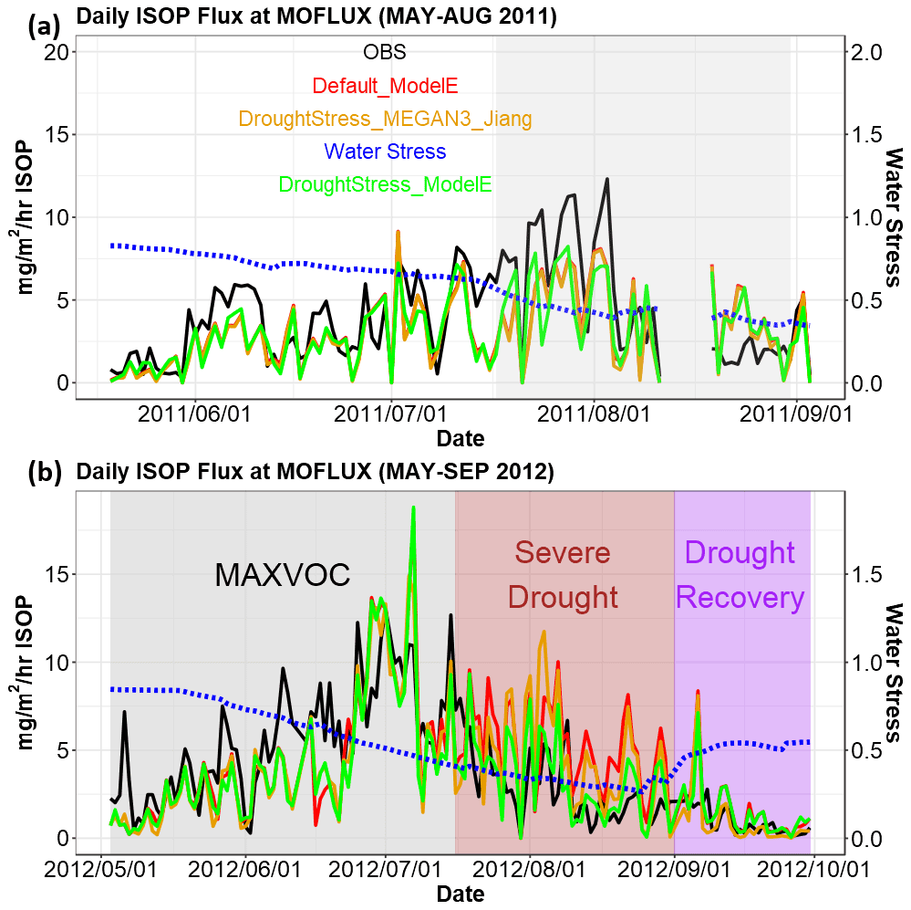
Figure 1 Daily isoprene emissions flux at MOFLUX (May–August 2011 and May–September 2012). LST time series are shown. Black shows observed isoprene emissions (abbreviated as ISOP), red shows Default_ModelE without isoprene drought stress, orange shows DroughtStress_MEGAN3_Jiang, and green shows DroughtStress_ModelE (units: mg m⁻² h⁻¹ of isoprene). (a) Shaded in grey from 17 July through 31 August 2011 is the period wherein water stress falls below 0.4 for short periods. (b) Shaded in grey is the MAXVOC period, shaded in brown is the period of severe–extreme drought from 17 July through August 2012, and shaded in purple is the drought recovery period.

In 2012, there were three unique periods that displayed the development of a severe drought that make it ideal to tune an isoprene drought stress algorithm. Shown in Fig. 1b is the daily averaged isoprene flux broken up into three periods. We define the MAXVOC episode from 1 May to 16 July. The severe drought period (17 July–31 August) is shaded in brown in Fig. 1b, and the drought recovery period is 1–31 September. Although Seco et al. (2015) defined MAXVOC from 18 June to 31 July, they identified 16 July as the transitional stage between the MAXVOC episode and severe drought. Thus, our work used 16 July to separate MAXVOC and severe drought periods. The periods of pre-drought (prior to 31 May) and mild drought identified by Seco et al. (2015) from 31 May to 14 June are included in the MAXVOC period because during this time period a typical seasonal pattern of increasing emissions with increasing temperatures is shown, and there is no indication of decreasing emissions due to drought stress. The mild drought period (31 May–14 June) corresponds to USDM periods of abnormally dry and moderate drought. Isoprene emissions continue to increase during the beginning of summer, which is supported by several studies showing that isoprene emissions during the first stages of drought increase even though there is a decrease in CO₂ fixation, which is attributed to drought-induced stomatal closure, rising leaf temperature, decreasing transpirational cooling, and CO₂ concentration in the leaf (Rosenstiel et al., 2003; Pegoraro et al., 2004; Potosnak et al., 2014; Seco et al., 2015). Separating the MAXVOC and severe drought period allows the algorithm development to target the latter severe drought stage wherein isoprene reduction occurs, while not reducing emissions during the early, and less severe, stages of drought. During the severe drought period, total annual precipitation was the lowest in a decade, while soil water content reached its minimum at the end of August when the drought peaked (Jiang et al., 2018). During the severe drought there is a marked decrease in isoprene flux, as shown by the brown shaded box coinciding with lower β values. It is well established that isoprene emissions are linked to high temperatures (Singsaas and Sharkey, 2000), and without the contributing factor of drought there should be an increase in isoprene emissions in July and August. The severe drought period encompasses periods of severe and extreme drought identified by the USDM. 3 July marks the first week indicated by the USDM of severe drought, and 31 July marks the first week of extreme drought. During severe drought isoprene production is suppressed by reductions in substrate availability and isoprene synthase transcription (Potosnak et al., 2014). Rain events at the end of August led to drought recovery and soil water content started to increase, which is indicated by increasing β values shown in the drought recovery period indicated in purple in Fig. 1b. Overall, 2012 shows a complete development of drought conditions that affect isoprene emissions and will provide useful constraints on the drought stress factor parameterization: a MAXVOC period that encompasses pre-drought and mild drought periods, a severe drought period (17 July–31 August), and a drought recovery period (1–30 September). Included in Fig. S8 are distributions of daily averaged isoprene flux split into MAXVOC, severe drought period, and drought recovery period for simulations Default_ModelE and DroughtStress_ModelE compared to observations.

2.6 Offline isoprene emissions model

An offline model was created based on the isoprene emissions formula in Eq. (4) of the MEGAN module contained in ModelE in order to develop the new parametrization in a timely fashion without waiting for online transient simulations to complete. ModelE was first run in a default transient simulation with MEGAN2.1 with no isoprene drought stress applied, which is referred to as Default_ModelE, from which the MEGAN activity factors and variables required to drive the offline calculation of isoprene emissions were output and archived. Default_ModelE is compared to observed temperature at MOFLUX in Figs. S10 and S12a as temperature is the main biogenic driver of isoprene (Mishra and Sinha, 2020; Jiang et al., 2018). Default_ModelE is also compared to sensible heat and latent heat in Fig. S11 as the exchange of latent and sensible heat fluxes is one of the most important aspects of land–atmosphere coupling. These energy fluxes are affected by partitioning of net radiation absorbed by the surface, which influences atmospheric dynamics, boundary layer structure, cloud development, and rainfall (Gu et al., 2016). We verified LAI at the MOFLUX site during 2012 in Fig. S12b using the NOAA Climate Data Record AVHRR (Advanced Very High Resolution Radiometer) LAI dataset (Vermote and NOAA CDR Program, 2019) that we averaged on a monthly scale and regridded from $\mathrm{0.05}{}^{\circ }\times \mathrm{0.05}{}^{\circ }$ to match ModelE's horizontal resolution. Other monthly averaged meteorological variables at MOFLUX during 2012, including temperature, LAI, relative humidity, shortwave incoming solar radiation, CO₂ flux, vapor pressure deficit (VPD), and canopy conductance, are compared to those observed when observations are available in Fig. S12. Soil moisture by layer is shown in Fig. S14. The offline model was then driven by these outputs at the half-hourly time step to match the 30 min time step in the online calculation of physics and the MEGAN module. The offline model was verified by making sure outputs of isoprene emissions matched the online Default_ModelE simulation. With the verified offline model, different parameterizations of isoprene drought stress could be tested and cross-verified with observations at MOFLUX. The offline model is used to derive a model-specific α and β threshold (Eqs. 6a–6c) for ModelE in order to create the appropriate parameterization of a model-specific isoprene drought stress in ModelE known as DroughtStress_ModelE, as described in Sect. 3.3. Since models calculate water stress and V_c,max in different ways, the offline model is the necessary step to derive model-specific water stress thresholds to target drought periods and ensure that α and β are being applied correctly.

2.7 ModelE sensitivity simulations

Four transient global ModelE simulations were configured for the period of 2003–2013 with a 3-year spin-up, as described in Table 1. A default simulation (Default_ModelE) that set y_d=1 was performed wherein no isoprene drought stress parameterization was applied. A second simulation named DroughtStress_MEGAN3_Jiang was performed as a sensitivity test to determine the efficacy of the DroughtStress_MEGAN3_Jiang algorithm in Eqs. (6a)–(6c), which is not tuned specifically for ModelE and was originally developed by Jiang et al. (2018) as a non-model-specific tuned isoprene drought stress formula to be widely used in models. A third simulation was performed based upon the offline-derived tuned response of ModelE to the best fit with MOFLUX observations (MOFLUX_DroughtStress) using Eqs. (8a)–(8c), as described in Sect. 3.2. A fourth simulation called DroughtStress_ModelE was performed using a subset of parameters derived from MOFLUX_DroughtStress but a different drought activation method (Sect. 3.3) using Eqs. (10a)–(10b).

Table 1 ModelE online transient simulation descriptions.

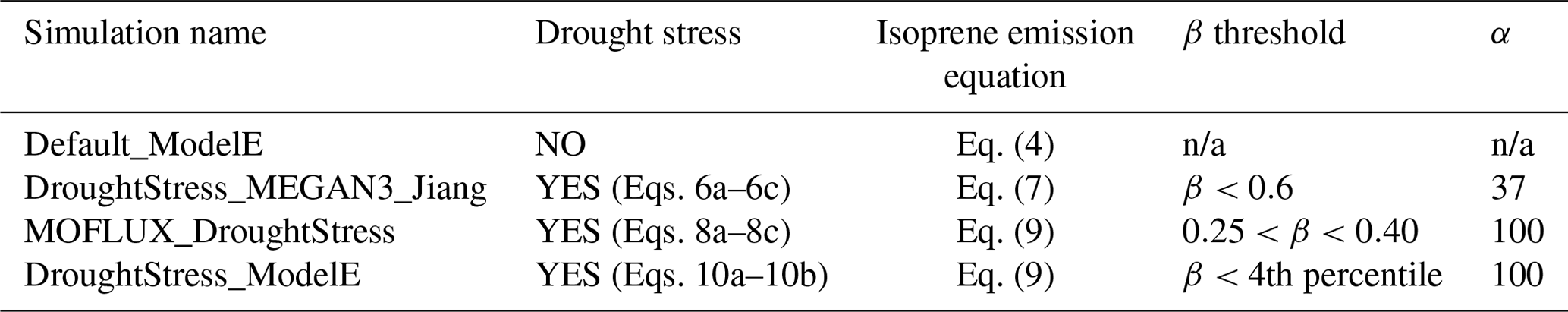
n/a: not applicable.

3 Development of model-specific drought stress parameterization

3.1 MOFLUX single-site observational comparison to model

Shown in Fig. 1a is the 2011 time series of biogenic isoprene flux at the MOFLUX site from the two online simulations Default_ModelE (red) and DroughtStress_MEGAN3_Jiang (orange) compared to observations (black). In 2011, Default_ModelE tended to underestimate isoprene flux during the onset of drought (14 July–10 August) and had minor periods of overestimation during drought progression (18 August–2 September), which was also seen by MEGAN2.1 simulations of Potosnak et al. (2014). The DroughtStress_MEGAN3_Jiang simulation applied isoprene drought stress from mid-July through September when β fell below the 0.6 threshold identified by Jiang et al. (2018). In the DroughtStress_MEGAN3_Jiang simulation it is shown that during the drought progression stage, DroughtStress_MEGAN3_Jiang isoprene is reduced compared to Default_ModelE, but reductions are not strong enough to align with lower observed values for a majority of this period. The time series shows that there is little deviation between Default_ModelE and DroughtStress_MEGAN3_Jiang during the 2011 mild drought.

Shown in Fig. 1b is the 2012 time series of biogenic isoprene flux at the MOFLUX site from the two online simulations Default_ModelE and DroughtStress_MEGAN3_Jiang compared to observations with β (blue). Default_ModelE typically underestimates isoprene flux during the MAXVOC period, overestimates during the severe drought period, and reproduces the drought recovery period sufficiently except for 6 September when the model greatly overestimates, leading to a peak not matched by observations. During the severe drought period the Default_ModelE mean bias (MB) ≅2.20 mg m⁻² h⁻¹ and the normalized mean bias (NMB) ≅76.10 %. β daily average values fell below the 0.60 threshold on 20 June and continued below the threshold through 3 September. With β falling below 0.60, the DroughtStress_MEGAN3_Jiang simulation starts reducing isoprene during the MAXVOC period and continues to reduce it through the drought recovery period. This leads to compounding the underestimation during the MAXVOC period, small corrections to overestimation during severe drought but missing peak overestimations, and overly large of reductions of isoprene during drought recovery period. During the severe drought period the MB of DroughtStress_MEGAN3_Jiang was ≅1.61 mg m⁻² h⁻¹ and the NMB was ≅55.81 %. DroughtStress_MEGAN3_Jiang thus decreased the overestimation by ∼20.29 % during the severe drought period. The time series comparison for 2012 indicates that the parameters in the Jiang et al. (2018) parameterization resulted in only minor improvements in ModelE for the severe drought period because they were tuned for CLM4.5. The DroughtStress_MEGAN3_Jiang simulation shows that α and β need to be tuned on a model-by-model basis. Based on these minor improvements and the differences in how V_c,max and β are calculated in CLM4.5 versus Ent TBM, it was clear a model-tuned parameterization could be used to further improve the relationship of simulated isoprene emissions during drought.

3.2 Site-tuned MOFLUX_DroughtStress parameterization

Using the offline isoprene emissions model (Sect. 2.6) driven by catalogued variables from each time step of the Default_ModelE simulation and the MOFLUX biogenic isoprene flux measurements for 2012, we describe here how a water stress threshold to target severe–extreme drought periods and a model-appropriate empirical variable (α) were derived to create the isoprene drought stress parameterization based upon the framework of Eqs. (6a)–(6c), called MOFLUX_DroughtStress. MOFLUX_DroughtStress was developed to target the 2012 severe drought period shown in Fig. 1b as this period is when the model overestimates despite observations showing decreasing emissions during drought. The water stress threshold range targeting the severe drought period determines when the isoprene drought stress is applied, and it is bounded to exclude the period of drought recovery and the onset of drought when isoprene emissions are still increasing. The range of β specific to ModelE is 0.25 to 0.40 during the severe drought period, which differs from the CLM4.5 threshold of 0.60 as it is a model-specific parameterization. Isoprene drought stress in MOFLUX_DroughtStress is thus applied only when $\mathrm{0.25}<\mathit{\beta }<\mathrm{0.40}$, and at all other β values y_d=1.

To find the empirical variable, α, an offline sensitivity analysis was conducted using the offline isoprene emissions model with 0.25 to 0.40 as the β threshold to activate isoprene drought stress. The PFT-weighted values of V_c,max and β were used to calculate the y_d in the offline isoprene emissions model. A range of α values from 60 to 160 was tested in Eqs. (8a)–(8c) to find y_d. y_d dependence on the value of α was fed into Eq. (9) to output offline isoprene emissions. The offline-modeled emissions from Eq. (9) were evaluated against observed isoprene fluxes at MOFLUX, and it was determined that α=100 gave the best fit and strongest relationship between the offline-modeled emissions and measured isoprene at MOFLUX. α=100 had the lowest NMB closest to zero during the severe drought period and the most improved slope, y intercept, and correlation coefficient during the summer of 2012. The α variable, though empirically derived, is strongly related to the model-specific V_c,max, which is why our alpha differs from DroughtStress_MEGAN3_Jiang, wherein α=37. Based on the offline emission comparisons to observed it was determined that MOFLUX_DroughtStress is defined as follows:

$$\begin{array}{}\text{(8a)}& {\displaystyle }{y}_{\mathrm{d}}=\mathrm{1}\left(\mathit{\beta }\ge \mathrm{0.4}\right),\text{(8b)}& {\displaystyle }{y}_{\mathrm{d}}={\displaystyle \frac{\left(v_{\mathrm{c},\max }\times \mathit{\beta }\right)}{\mathit{\alpha }}}\left(\mathrm{0.25}<\mathit{\beta }<\mathrm{0.40}\right)\text{where}\mathit{\alpha }=\mathrm{100},\text{(8c)}& {\displaystyle }{y}_{\mathrm{d}}=\mathrm{1}\left(\mathit{\beta }\le \mathrm{0.25}\right),\end{array}$$

$$\begin{array}{}\text{(9)}& \begin{array}{rl}{\text{isoprene}}_i=& \left(\mathrm{1}\times {\mathrm{10}}^{-\mathrm{9}}/\mathrm{3600}\right)\\ & \times \left({\text{EF}}_{i,\mathrm{isoprene}}\times {\text{PFTboxf}}_i\right)\times y_{\mathrm{LAI}}\times y_{\mathrm{A}}\\ & \times y_{\mathrm{d}}\times y_{{\mathrm{CO}}_{\mathrm{2}}}\times \left(y_{\mathrm{P}}\times y_{\mathrm{TLD}}\right)\times {\text{SF}}_{\mathrm{isoprene}},\end{array}\end{array}$$

where y_d uses the area-weighted average over PFTs of V_c,max and β in Eqs. (8a)–(8c), and thus y_d in Eq. (9) is not a function of PFT, which differs from DroughtStress_MEGAN3_Jiang in Eq. (7) where y_d is a function of PFT.

MOFLUX_DroughtStress simulation with isoprene drought stress applied in Eqs. (8a) to (8c) is found to reduce the MB at the MOFLUX site to ≅0.04 mg m⁻² h⁻¹ during the 2012 severe drought period, indicating that the parameterization is able to correct the model overestimation of isoprene emissions. Scatterplots and time series of the simulation MOFLUX_DroughtStress during May–September 2012 are included in Fig. S2. The NMB decreased to ≅1.53 %, indicating a ∼74.57 % reduction compared to Default_ModelE. Large improvements were not expected for 2011 as this algorithm was designed to target severe–extreme drought. Despite the better agreement between measured and modeled fluxes in MOFLUX_DroughtStress at the MOFLUX site, the regional analysis described below determined that water stress values are region-specific and a new approach was needed in order to make the algorithm applicable for other regions in the global model.

3.3 New percentile threshold isoprene drought stress parameterization

After implementing MOFLUX_DroughtStress in ModelE, we found isoprene emissions reductions for June–August 2011 in the southeastern (SE) US (defined as 96–75^∘ W, 25–38^∘ N) of approximately −3.5 %, −7.2 %, and −5.7 %, respectively. These regional reductions were smaller than expected as the SE US in 2011 experienced a spatially extensive severe drought over a largely forested and vegetated region. The US Drought Monitor (USDM) reported that in June–August 2011 63 %, 61 %, and 55 %, respectively, of the southeast area was in moderate to exceptional drought. Other studies for other regions of the world have reported during severe drought that reductions in isoprene vary by region and have large uncertainty. For example, Huang et al. (2015) reported that using different soil moisture products resulted in isoprene reductions of 12  %–70 % for Texas. Others showed reductions up to a maximum of 17 % (Jiang et al., 2018; Wang et al., 2021). The reason why MOFLUX_DroughtStress falls on the lowest end of reported isoprene reductions for the regional analysis is probably because drought stress activation was calibrated to water stress ranges at a single site. As water stress is expected to vary regionally, a new regional method was needed in order to simulate drought stress effects globally.

A new parameterization was designed to not only work at MOFLUX since this is the site used for validation, but also capture isoprene drought signals for other regions. To do so, we first simulated daily averaged water stress during the growing season for 10 years (2003–2012) at MOFLUX for a total of 2450 d. It was determined that water stress was less than the 0.4 threshold for 102 d, which is a percentage of ∼4.16 %. For simplicity, we rounded the percentage to 4 %. The new approach then relied upon finding the fourth percentile water stress value across 10 years of daily water stress per grid and for each individual month in order to build a parameterization that would capture regional and seasonal variability in water stress in ModelE. This new drought stress parameterization is known as DroughtStress_ModelE, uses the same alpha (α=100) as MOFLUX_DroughtStress, and is applied as weighted average per PFT. What makes this different from the previous approach, MOFLUX_DroughtStress, is that the water stress threshold used to apply drought stress is based on the model's unique lowest fourth percentile of water stress on a grid-by-grid basis, is not based on the absolute values of water stress at a single site (i.e., MOFLUX), and is a statistical tuning method. The fourth percentile of daily water stress was used as the trigger for drought stress activation. The parameterization for DroughtStress_ModelE is Eqs. (10a)–(10b):

$$\begin{array}{}\text{(10a)}& {\displaystyle }{y}_{\mathrm{d}}=\mathrm{1}\text{when}\left(\mathit{\beta }\ge \mathrm{4}\text{th percentile}\right),\text{(10b)}& {\displaystyle }\begin{array}{rl}{y}_{\mathrm{d}}=& {\displaystyle \frac{\left(v_{\mathrm{c},\max }\times \mathit{\beta }\right)}{\mathit{\alpha }}}\text{when}\left(\mathit{\beta }<\mathrm{4}\text{th percentile}\right),\\ & \text{where}\mathit{\alpha }=\mathrm{100}.\end{array}\end{array}$$

A global transient simulation was run (2003–2013) by applying Eqs. (10a)–(10b) globally, called DroughtStress_ModelE in order to determine the effects of the isoprene drought stress parameterization and to see if it captures the signal of the 2011 SE drought. DroughtStress_ModelE for JJA 2011 showed isoprene emissions percent reductions for the SE of approximately −9.6 %, −5.9 %, and −12.7 %, respectively. These reported reductions are a factor of 2 greater than MOFLUX_DroughtStress for the same period and are in the mid-range of reported isoprene reductions during drought. A complete time series of isoprene emissions at MOFLUX for all four simulations as described by Table 1 is shown in Fig. S2a–b for 2011 and 2012.

3.4 DroughtStress_ModelE evaluation at MOFLUX

During 2011 at the MOFLUX site, there were only small differences between Default_ModelE and DroughtStress_ModelE. The scatterplots of isoprene emissions at the MOFLUX site for the summer of 2011 show that the hourly correlation coefficient between modeled and observed isoprene fluxes experienced minor improvement from 0.77 to 0.78, with minor changes in slope and y intercept (Fig. S3a, c). The diurnal cycles for 2011 included in Fig. S4a show that neither MOFLUX_DroughtStress nor DroughtStress_ModelE altered the diurnal cycle in comparison to Default_ModelE. For 2011, all four simulations underestimate the diurnal cycle for May–August. Large improvements due to the applications of the Eqs. (10a)–(10b) were not expected for 2011 as this algorithm was designed to target severe–extreme drought and not less severe drought conditions.

During the severe drought period of 2012 at MOFLUX, the β values fell below the fourth percentile thresholds for July–August, and isoprene drought stress was applied, leading to reductions in the overestimation shown by Default_ModelE. DroughtStress_ModelE had MB ≅0.42 mg m⁻² h⁻¹ and NMB ≅14.5 % during the severe drought period. DroughtStress_ModelE reduced overestimation by ∼61.6 % during the severe drought period compared to Default_ModelE, which is a similar statistical improvement compared to MOFLUX_DroughtStress during the severe drought period as the parameterizations were designed in a similar manner. The scatterplots of isoprene emissions at the MOFLUX site for the summer of 2012 show that the hourly correlation coefficient between observations and simulations increased from 0.68 in Default_ModelE to 0.73 in DroughtStress_ModelE (Fig. 2a, c). In Fig. 2 changes are clearly seen in the cluster of β values lower than 0.4 (shown by red oval), indicating a reduction in overestimation during severe drought.

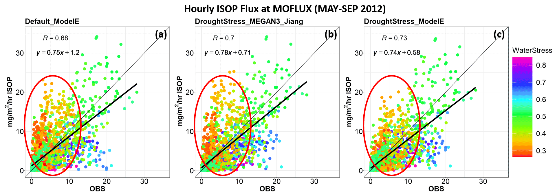
Figure 2 Scatterplots (a)–(c) show hourly simulated isoprene emissions compared to observed for May–September 2012 at the MOFLUX site (units: mg m⁻² h⁻¹ of isoprene). Panels (a)–(c) indicate the simulations Default_ModelE, DroughtStress_MEGAN3_Jiang, and DroughtStress_ModelE, respectively. The hourly averaged points are color-coded by water stress.

DroughtStress_ModelE, with decreases in y intercept, increasing correlation coefficient, and minor change in slope compared to Default_ModelE, suggests better performance in simulating isoprene emissions during severe and extreme drought at MOFLUX during the summer of 2012. The hourly scatterplots during the 2012 severe drought period are included in Fig. S13. The daily correlation coefficient increased from 0.64 to 0.73 during the 2012 drought in DroughtStress_ModelE (Fig. S5a, c), and in Fig. S13 during the severe drought period the daily correlation increases from 0.40 to 0.48. In addition, DroughtStress_ModelE reproduces the diurnal cycle of isoprene emission from May–September 2012, as shown in Fig. S4b, and corrects the overestimation of Default_ModelE during the peak hours of 10:00–15:00 LST. It was found that DroughtStress_ModelE tended to reduce the overestimation of Default_ModelE for the daily peak of isoprene flux and move it closer to observed during the severe drought period, as shown in Fig. S9. Overall, there is an acceptable level of agreement between measured and modeled fluxes in DroughtStress_ModelE, indicating that it is a suitable model-tuned parameterization for estimating isoprene emissions during severe drought at the MOFLUX site.

4 Model response to drought parameterization: global and regional evaluation of DroughtStress_ModelE

The impact of applying isoprene drought stress in DroughtStress_ModelE globally to the annual emissions of isoprene from 2003–2013 is shown in Table 2. The yearly global reduction of isoprene emissions ranges from $\sim -\mathrm{0.9}$ % to −4.3 %. The global decadal average from 2003–2013 is ∼533 Tg yr⁻¹ of isoprene in Default_ModelE and ∼518 Tg yr⁻¹ of isoprene in DroughtStress_ModelE, which is a reduction of 2.7 %, which is equivalent to ∼14.6 Tg yr⁻¹ of isoprene. On a global scale these changes average under 3 %, but for high-isoprene-emission regions such as the southeastern US during drought periods there are larger impacts, as shown below in Fig. 6.

Table 2 Global annual Tg of isoprene (2003–2013).

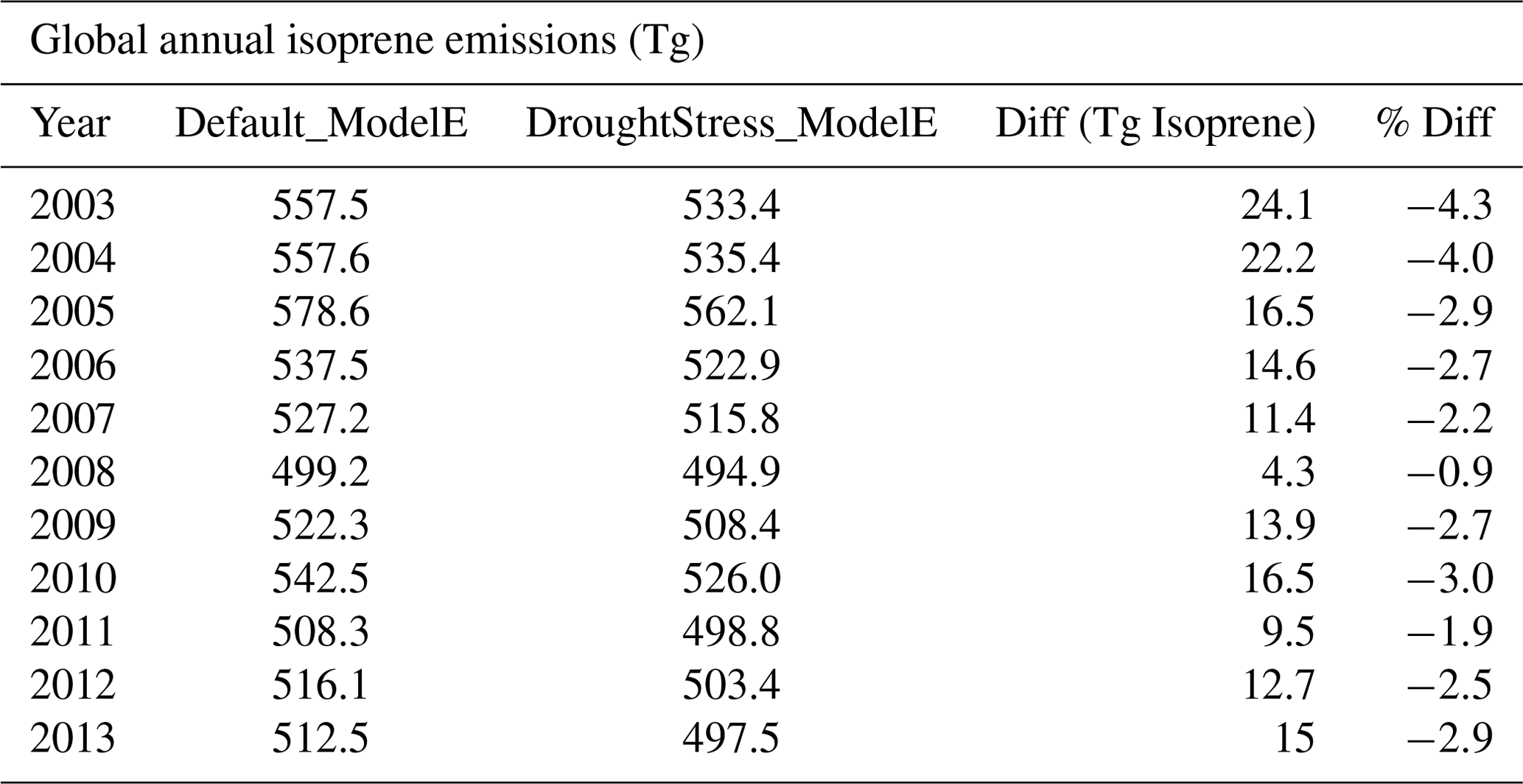
Figure 3 shows the global 9-year average of isoprene emissions and tropospheric HCHO column densities (ΩHCHO) of the lowest 20 layers of the model during JJA from 2005–2013. Due to extremely limited in situ measurements of isoprene emissions during drought, satellite-retrieved ΩHCHO, which is the high-yield oxidation product of isoprene, can be used as a proxy for isoprene emissions on the monthly scale (Zhu et al., 2016). Here we used ΩHCHO from OMI (Ozone Monitoring Instrument) on the Aura satellite starting in 2005. The level 3 total column-weighted mean was regridded from its original resolution of $\mathrm{0.1}{}^{\circ }\times \mathrm{0.1}{}^{\circ }$ to match ModelE's horizontal resolution of $\mathrm{2}{}^{\circ }\times \mathrm{2.5}{}^{\circ }$, and the daily data were aggregated to a monthly mean (Chance, 2019). OMI satellite data were filtered with the data_quality_flag, so cloud fractions less than 0.3, solar zenith angles less than 60, and values within the range of −0.5 to 10×10¹⁶ molec. cm⁻² were used (Zhu et al., 2016). A factor of 1.59 is applied to the OMI vertical column density (VCD) to correct the mean bias (Kaiser et al., 2018). As this is the first evaluation of tropospheric ΩHCHO in ModelE, a gridded level 3 dataset was used for analysis without applying the air mass factor (AMF) using ModelE-predicted HCHO profiles, which according to Zhu et al. (2016) can lead to an increase of ∼38 % uncertainty in the southeastern US. Figure 3c and f show the percent difference of isoprene emissions and ΩHCHO, and shown in blue are the decreases in DroughtStress_ModelE globally. Figure 3d–e show OMI ΩHCHO and Default_ModelE-simulated ΩHCHO. It is important to note the difference in scales as Default_ModelE overestimates ΩHCHO in regions such as the SE US for every June–July from the 2005–2013 period with a regional mean scale factor of ∼0.56 and ∼0.80 when the SE boundary is extended westward to include portions of Texas. These overestimates in the SE US are also reported by Kaiser et al. (2018) wherein they saw a 50 % overestimate by GEOS-Chem with MEGAN2.1 simulations compared to SEAC⁴RS observations. While applying isoprene drought stress leads to reductions in ΩHCHO as shown by Fig. 3f, this reduction is limited to drought-stricken regions and periods, and it is not designed to correct for the systematic biases of HCHO in ModelE. The overestimation of ΩHCHO in Default_ModelE will require further study and could be due to several reasons such as emission errors, incorrect spatial gradients of OH, or possibly an overly strong sensitivity to temperature (Wells et al., 2020; Zhu et al., 2017; Wang et al., 2022). This version of ModelE also lacks direct emissions of HCHO from anthropogenic sources, which may result in the lower vertical deposition and, due to the short lifetime, the higher than the observed HCHO column over portions of the US and lower in other regions. It was found that nudged simulations show a large overestimation of the HCHO column compared to free-running simulations using model winds. As this study only shows modest decreases in the HCHO column we can only conclude that adding isoprene drought stress to a model may reduce the HCHO column depending on atmospheric chemistry, but under certain NO_x- and VOC-limited environments may have another effect.

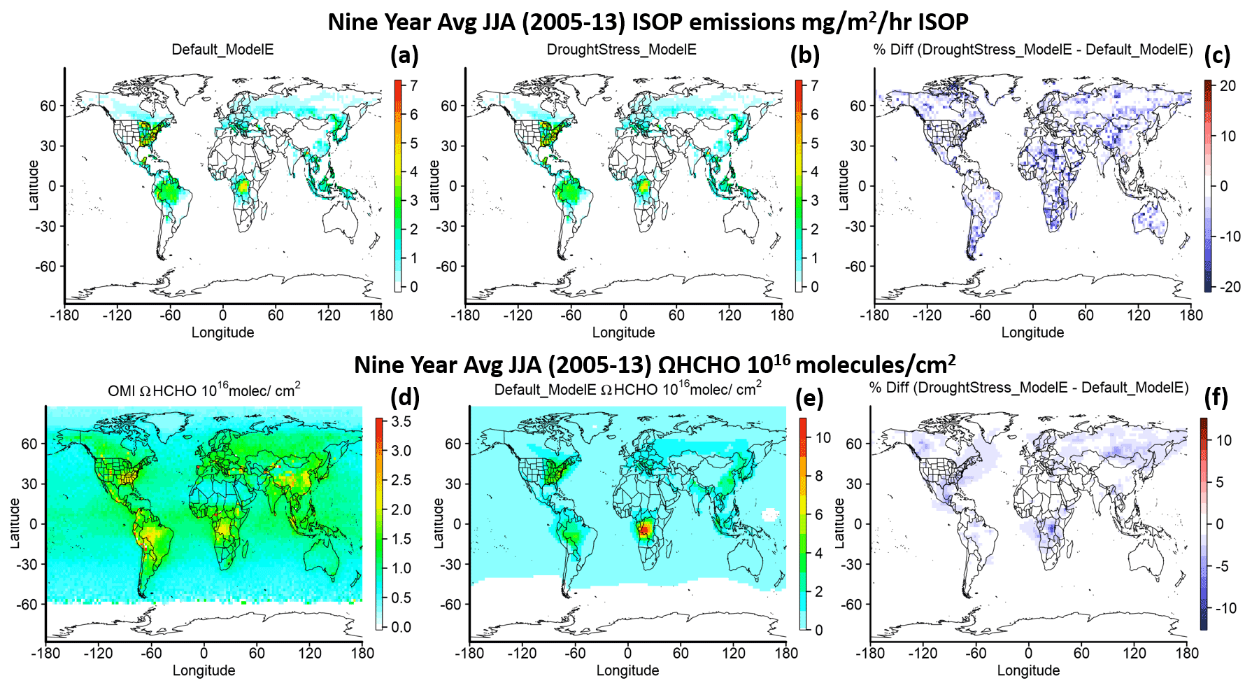
Figure 3 Global 9-year average of JJA 2005–2013 isoprene emissions (first row) for Default_ModelE (a), DroughtStress_ModelE (b), and the percent difference between DroughtStress_ModelE and Default_ModelE (c). ΩHCHO (second row) for OMI (d), Default_ModelE (e), and the percent difference between DroughtStress_ModelE and Default_ModelE (f). Note the different color scales between panels (d) and (e).

Four global isoprene emission hotspots are selected to showcase the changes in isoprene emissions. The geographic regions are defined as the eastern US (eastern US: 65–105^∘ W, 25–50^∘ N), SA (Amazon: 40–80^∘ W, 30^∘ S–7^∘ N), AF (central Africa: 10–40^∘ E, 15^∘ S–10^∘ N), and SE Asia (Southeast Asia: 100–150^∘ E, 11^∘ S–38^∘ N) as shown in Fig. S6. Figure 4 shows the relationship of dryness categorized by SPEI (Standardized Precipitation–Evapotranspiration Index) and relative difference in isoprene emissions between DroughtStress_ModelE and Default_ModelE from 2005–2013 for the growing season in the Northern Hemisphere and spring–summer in the Southern Hemisphere for the four global isoprene hotspots. SPEI is a multiscalar climatic index that represents the duration of drought in a region. It is based on a climatic water balance approach which considers the impact of temperature and evapotranspiration (Beguería et al., 2010; Vicente-Serrano et al., 2010; Beguería et al., 2014). To identify the extent of drought impacts and differentiate from normal variability in the hydrological cycle, 1-month SPEI is used to identify drought periods extending beyond a single month. Default_ModelE simulation variables were used to calculate modeled SPEI at the resolution of $\mathrm{2}{}^{\circ }\times \mathrm{2.5}{}^{\circ }$. Positive SPEI typically indicates wet conditions, and dry conditions are indicated by negative values. Drought conditions are indicated by SPEI $\le -\mathrm{1.3}$, normal conditions $-\mathrm{0.5}\le \text{SPEI}\le \mathrm{0.5}$, and wet conditions SPEI ≥1.3 following the Wang et al. (2017) approach. For the four regions the average percent difference in isoprene emissions for March–October for Northern Hemisphere regions and September–February for Southern Hemisphere regions from 2005–2013 is $\sim -\mathrm{2.62}$ % for the eastern US, $\sim -\mathrm{3.01}$ % for the Amazon (SA), $\sim -\mathrm{2.64}$ % for central Africa (AF), and $\sim -\mathrm{3.10}$ % for Southeast Asia (SE Asia). The scatterplots for the four hotspots show decreasing isoprene emissions across all dryness conditions. The decreases in isoprene emissions for the four regions are not seen exclusively when SPEI indicates dry conditions, which indicates the simulated water stress as shown by the model does not exactly align with SPEI drought-indicated conditions.

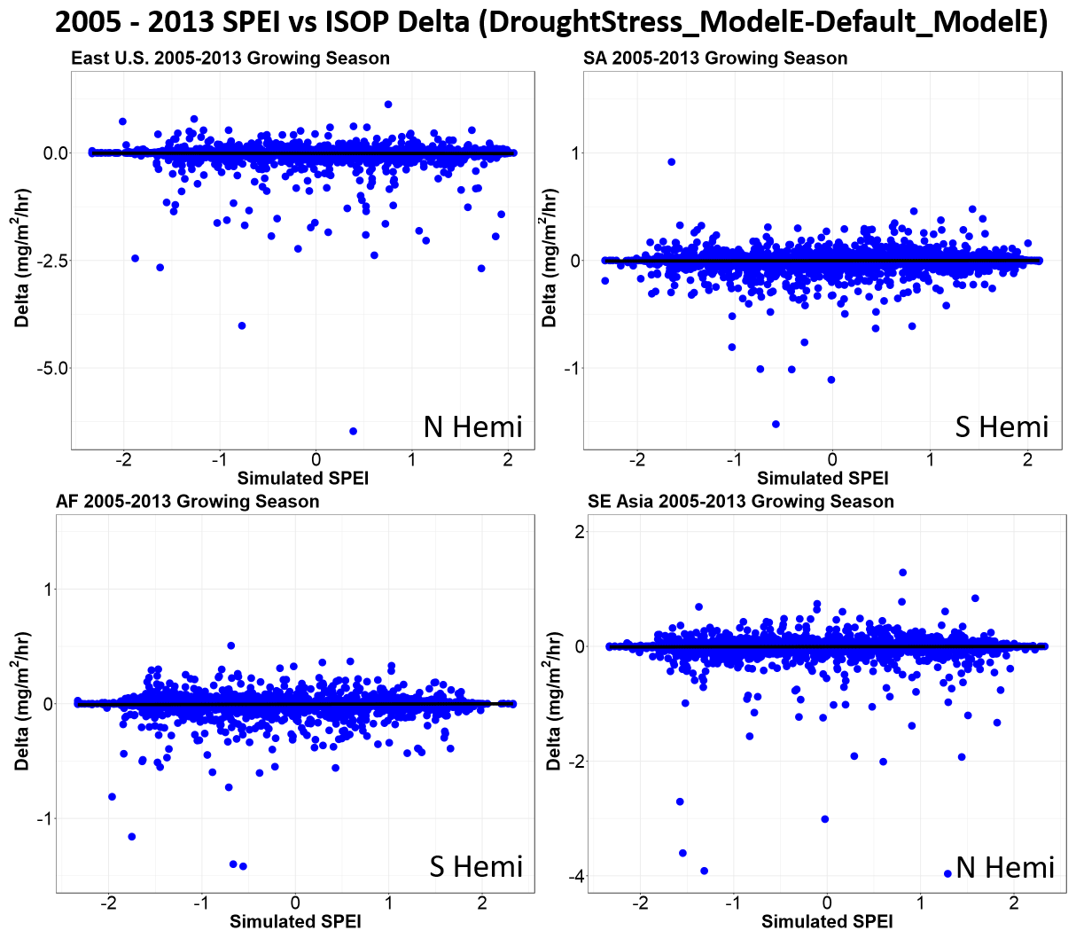
Figure 4 Scatterplots of four global isoprene hotspots and their relative differences in isoprene emissions (mg m⁻² h⁻¹ isoprene) in relationship to simulated SPEI from 2005–2013 during the growing season. The four regions of focus are the eastern US (East), the Amazon (SA), central Africa (AF), and Southeast Asia (SE Asia). The regions East and SE Asia are in the Northern Hemisphere, and the growing seasons is from March–October. The hotspots of SA and AF are in the Southern Hemisphere, and the growing season is during spring–summer (September–February).

Narrowing the focus from global to the US to illustrate the long-term difference between DroughtStress_ModelE and Default_ModelE, a time series from 2005–2013 is shown in Fig. 5 of the continental US for the two regions West (105–125^∘ W, 25–50^∘ N) and East (65–105^∘ W, 25–50^∘ N), indicating the percent difference in ΩHCHO and isoprene emissions corresponding to percent area that is dry (SPEI $<-\mathrm{0.5}$). The map showing the regions West and East is located in Fig. S7. The western US (West), despite having a much smaller magnitude of isoprene emissions, does see reductions in isoprene, which is mimicked on a lesser scale by reductions in ΩHCHO. For the eastern US (East) there are visible decreases in the percent reduction of isoprene emission and ΩHCHO during the 2007, 2011, and 2012 drought years. Focusing on the East time series, the maximum percent difference between simulations DroughtStress_ModelE and Default_ModelE for isoprene occurred from August–October 2007 of approximately −4.5 %, −7.4 %, and −4.6 %, with corresponding decreases in ΩHCHO of $\sim -\mathrm{4.1}$ %, −5.4 %, and −3.6 %, respectively. For 2011 the maximum percent difference in isoprene emissions occurred in September–November and was $\sim -\mathrm{9.0}$ %, −8.7 %, and −8.3 %. The percent difference in ΩHCHO was $\sim -\mathrm{5.9}$ %, −3.6 %, and −2.6 %. For 2012 the maximum percent difference occurred from August–October, and the difference in isoprene was $\sim -\mathrm{5.1}$ %, −8.8 %, and −10.8 %. The difference in ΩHCHO was $\sim -\mathrm{2.8}$ %, −4.0 %, and −2.7 %.

Figure 5 The percent difference of ΩHCHO and isoprene emissions from 2005–2013 in relationship to percent area dry for two regions of the US: West (a) and East (b). Percent dry area is indicated by SPEI $<-\mathrm{0.5}$. The first grey shaded rectangle indicates the time period of the 2011 drought at MOFLUX from June to August 2011. The second grey shaded rectangle indicates the 2012 severe drought at MOFLUX from 17 July through August. These time periods are added to the time series to highlight when they occurred.

Figure 6 displays spatial maps of ΩHCHO during the summer (JJA) of 3 drought years: 2007, 2011, and 2012. The summers of 2007 and 2011 were drought periods in the US, with 2007 being a less severe drought than 2011 in the SE US. The drought of 2012 was focused more on the Great Plains (GP) region. The spatial maps show the reduction in ΩHCHO in panels (c), (f), and (i) due to the inclusion of isoprene drought stress. Based on the spatial differences in ΩHCHO, three regions of the greatest reduction in percent difference in the ΩHCHO column are selected for the 3 drought years of 2007, 2011, and 2012, respectively. The three geographic regions are shown in Fig. 7 and defined as SE1 (Southeast Region1: 75–93^∘ W, 31–39^∘ N), SE2 (Southeast Region2: 75–101^∘ W, 29–37^∘ N), and GP (Great Plains: 89–100^∘ W, 33–43^∘ N). During JJA for 2007 the SE1 region has an average percent difference in ΩHCHO of −6.46 %. During JJA 2011 the SE2 region has a percent difference of −7.58 %, and the GP region during JJA 2012 has an average percent difference of −3.29 %.

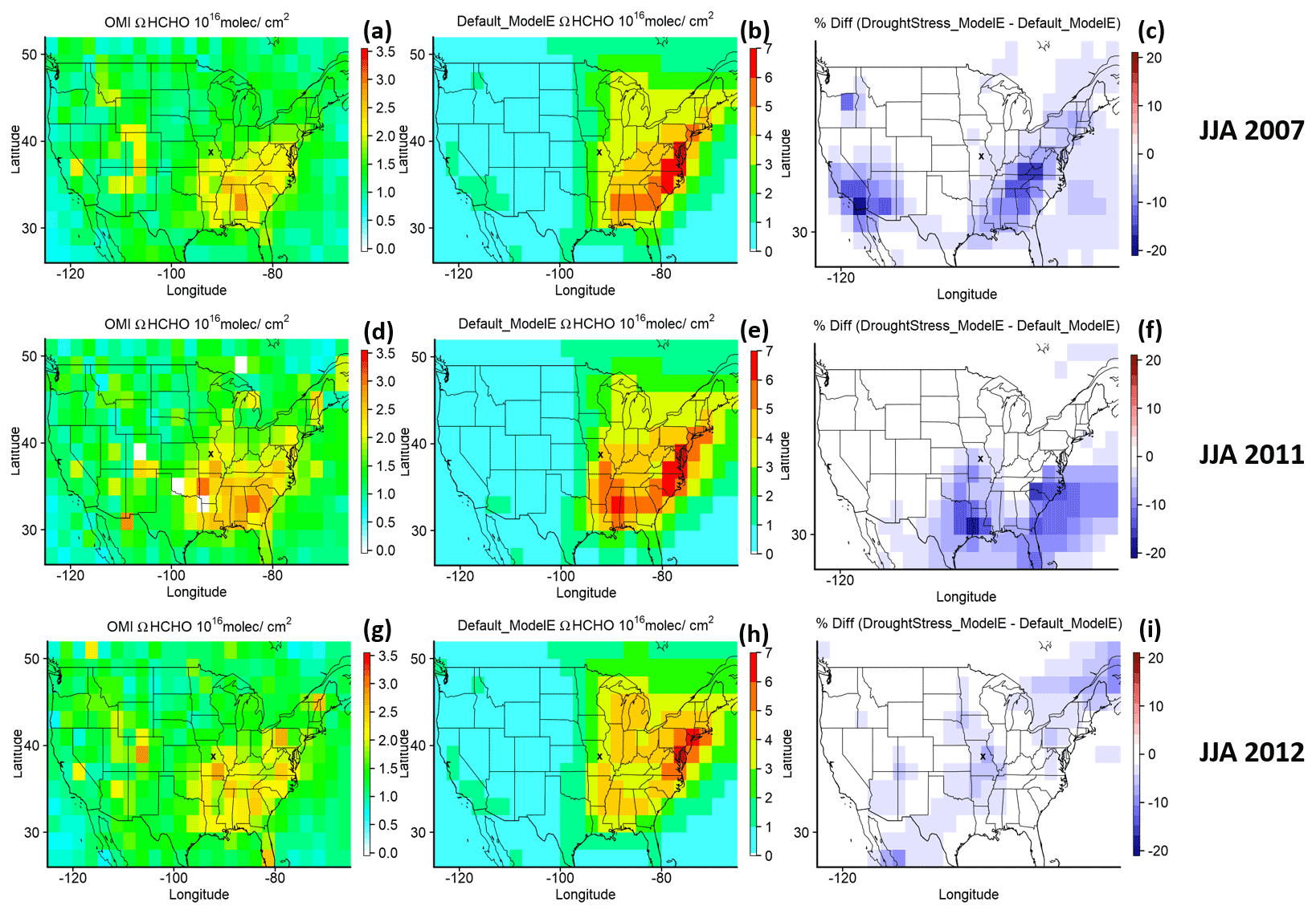
Figure 6 The ΩHCHO column (units: molec. cm⁻²) for OMI, Default_ModelE, and the percent difference between DroughtStress_ModelE and Default_ModelE across the US during the summer of drought years 2007, 2011, and 2012. X indicates the location of the MOFLUX site on the spatial maps.

Figure 7 shows the time series for the three regions of SE1 during 2007, SE2 for 2011, and GP for 2012. In the SE1 region during the period of maximum isoprene difference from August–October 2007 (shaded in grey on the time series), DroughtStress_ModelE reduced NMB of ΩHCHO by ∼19.3 %. The isoprene percent difference for this period was approximately −9.0 %, −17.5 %, and −13.2 %. The ΩHCHO percent difference for the SE1 region from August–October 2007 was approximately −8.4 %, −12.1 %, and −7.3 %. In the SE2 region the maximum isoprene difference period was August–November 2011, and DroughtStress_ModelE decreased ΩHCHO NMB by ∼15.3 %. The monthly isoprene percent difference for SE2 during this period was approximately −16.1 %, −18.6 %, −14.7 %, and −13.9 %, while the ΩHCHO percent difference was $\sim -\mathrm{10.0}$ %, −11.2 %, −6.6 %, and −4.6 %, respectively. In the GP region during September–November 2012, the isoprene percent difference was approximately −5.4 %, −14.2 %, and −11.1 %, and the ΩHCHO percent difference was $\sim -\mathrm{2.8}$ %, −2.4 %, and −0.4 %, respectively. The small change in the HCHO column despite estimated larger changes in isoprene emissions is probably due to the suppression of oxidants such as hydroxyl radicals (OH) by isoprene under low-NO_x conditions in the GP region (Wells et al., 2020).

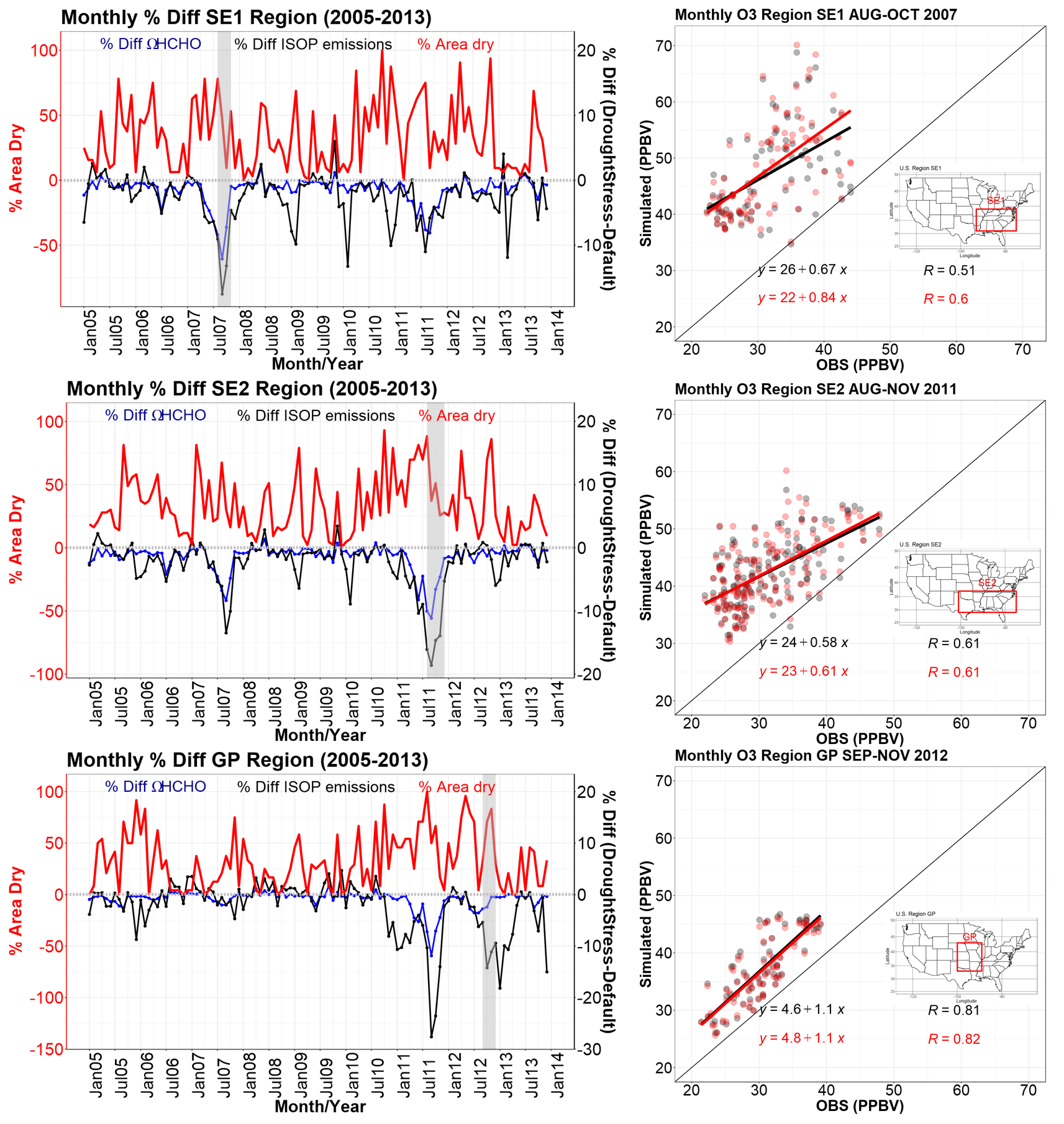
Figure 7 The time series from 2005–2013 of percent dry area on the y axis shown in red and the percent difference in ΩHCHO (blue) and isoprene emissions (black) between DroughtStress_ModelE and Default_ModelE for the three regions SE1, SE2, and GP on the second y axis. Shaded in grey are the time periods of the maximum percent difference of isoprene emissions during the drought years. The scatterplots show the relationship between observed O₃ (ppbv) and simulated O₃ during the shaded grey time periods on the time series for Default_ModelE in black and DroughtStress_ModelE in red for SE1 during 2007, SE2 during 2011, and GP during 2012. Maps showing the geographic regions are inset into the scatterplots. The regions' spatial extent is based on the region of maximum percent difference in Fig. 6c, f, and i.

It is well established that biogenic isoprene, the most abundant BVOC, is a highly reactive species. In the presence of nitrogen oxides (NO_x), BVOCs contribute to the formation of tropospheric O₃. Oxidation of BVOCs also produces secondary organic aerosols, a major component of fine particulate matter (PM_2.5). PM_2.5 and O₃ have been previously linked to change during drought with adverse effects on air quality (Wang et al., 2017). During drought there is elevated O₃ and PM_2.5 compared to non-drought periods (Wang et al., 2017; Zhao et al., 2019; Naimark et al., 2021). Higher ozone compared to non-drought years is due to the reduction of vegetative deposition due to reduced stomatal conductance, higher temperatures stimulating precursors, and enhanced NO₂ (Naimark et al., 2021). By including isoprene drought stress in the simulations, isoprene emissions are decreased, which will change O₃; the direction of change depends on NO_x-limited or VOC-limited regimes (Li et al., 2022). In summary, we better predicted isoprene emission response to drought by including isoprene drought stress. It is thus important to show the impact of drought-induced changes in isoprene emissions on O₃ and PM_2.5. The scatterplots in Fig. 7 show the relationship between observed and simulated O₃ during the drought period of maximum percent difference highlighted on the time series for the corresponding region. PM_2.5 comparison to observed is not shown here due to Default_ModelE underestimating PM_2.5 across all three regions SE1, SE2, and GP, and thus no improvements were seen due to the inclusion of DroughtStress_ModelE. The observational O₃ data are a combination of hourly data from the EPA-AQS (US Environmental Protection Agency, EPA, Air Quality System), CASTNET (Clean Air Status and Trends Network), and NAPS (National Air Pollution Surveillance) networks. The observational O₃ datasets were gridded and interpolated for comparison to a gridded model (Schnell et al., 2014). The hourly gridded observations were then averaged onto a monthly scale for comparison with model results. Shown in Fig. 7, the SE1 region saw improvement in O₃ from August–October 2007 when the correlation coefficient (R) increased from 0.51 in Default_ModelE to 0.60 in DroughtStress_ModelE, and the slope of the linear regression also improved significantly. The SE2 region from August–November 2011 saw a slight improvement in the slope of the linear regression but no change in R. The GP region from September–November 2012 saw a slight improvement in R but no change in the correlation slope between Default_ModelE and DroughtStress_ModelE. During non-drought periods of 2008, 2010, and 2013 compared to their respective drought periods of 2007, 2011, and 2012 there were no large changes in O₃ or ΩHCHO statistics as expected since isoprene drought stress is only supposed to affect drought periods. During the drought periods of 2007, 2011, and 2012 the model predicts higher mean O₃ and ΩHCHO than the non-drought years of 2008, 2010, and 2013. The analysis of these drought years and periods of the greatest percent difference leads to the conclusion that isoprene drought stress improves ΩHCHO simulation and O₃ simulation during drought periods.

5 Discussion and conclusions

Drought is a hydroclimatic extreme that causes perturbations to the terrestrial biosphere. As a stressor for vegetation, drought can induce changes to vegetative emissions known as BVOCs (biogenic volatile organic compounds). Biogenic isoprene represents about half of total BVOC emissions and is a precursor to ozone (O₃) and secondary organic aerosol (SOA), both of which are climate forcing species. In order to simulate isoprene flux during drought and the feedbacks associated with these complex BVOC–chemistry–climate interactions, we implemented the MEGAN (Model of Emissions of Gases and Aerosols from Nature) isoprene drought stress parameterization, y_d, into NASA GISS (Goddard Institute of Space Studies) ModelE, a leading Earth system model. Four online transient simulations were performed from 2003–2013: Default_ModelE without y_d, DroughtStress_MEGAN3_Jiang using the parameterization developed by Jiang et al. (2018), and a model-tuned parameterization developed for ModelE based on the MOFLUX AmeriFlux site observations (MOFLUX_DroughtStress). The fourth simulation implemented isoprene drought stress using a grid-by-grid approach to capture regional changes in isoprene during drought known as DroughtStress_ModelE. The model-tuned parameterization (MOFLUX_DroughtStress and DroughtStress_ModelE) was developed using an offline model of emissions to create a model-specific empirical variable and water stress threshold, since key variables V_c,max (photosynthetic parameter) and water stress (β) are parameterized differently across models. Observational measurements of isoprene flux during the severe drought of 2012 at the MOFLUX site were used for validation of the parameterization. It was found that DroughtStress_ModelE corrects the overestimation of emissions during the phase of severe drought at MOFLUX. Previously, this reduction during drought was not included in BVOC emission models due to the lack of a drought stress term. Globally the decadal average from 2003–2013 in Default_ModelE was ∼533 Tg of isoprene and ∼518 Tg of isoprene in DroughtStress_ModelE. DroughtStress_ModelE was validated using the observational satellite ΩHCHO column from the Ozone Monitoring Instrument (OMI) and using O₃ observations across regions of the US to examine the effect of drought on atmospheric composition. It was found that the inclusion of isoprene drought stress reduced the overestimation of ΩHCHO in Default_ModelE during the 2007 and 2011 southeastern US droughts and led to improvements in simulated O₃ during drought periods. The inclusion of a grid-specific percentile isoprene drought stress is model-specific, and the reduction of isoprene seen in models will depend on each model's mean bias and parameterizations of V_c,max and water stress. ModelE's modest signal can be explained by underestimating isoprene emissions during the early stages of drought and by not having a high mean bias during severe drought.

Our analysis of isoprene drought stress leads to the recommendation that each model should arrive at a tuning of their water stress parameters based on the magnitude of water stress occurring during simulated drought, and a unique alpha should be derived. Each land surface model (LSM) has a unique hydrology scheme (with different soil layering approaches and soil physics treatments), and any variables that depend on response to soil moisture – whether chemical, physical, or biological – must be tuned due to the fact that soil moisture in LSMs is averaged over a grid cell, whereas in nature soil moisture is heterogeneous at spatial scales down to the plot level. The resulting parameterization, since it relies on model-specific variables, would be well suited for future or historical simulations. The current approach also requires vegetation-coupled land surface models that have photosynthesis models that use V_c,max and β, and many current general circulation models (GCMs) with less process-based vegetation schemes do not have these variables readily available.

Besides tuning responses to drought, the light response of isoprene emissions may not be well captured in a simple factor like the PCEEA. Vegetation models differ in their approach to leaf-to-canopy scaling. Some ESMs' vegetation models have more sophisticated canopy radiative transfer submodels that capture layering and sunlit–shaded leaf area. Future isoprene modeling investigations could make use of the ability of these canopy models to calculate isoprene emissions with leaf-level responses to the heterogeneous light in canopies. Unger et al. (2013) previously implemented such a leaf-to-canopy scaling of isoprene emissions in the Ent TBM through a leaf-level isoprene model as a function of leaf-level gross primary production (GPP). Since the Ent TBM scales stomatal conductance with drought stress and hence also GPP, this intrinsically results in isoprene emission responsiveness to drought stress. The main challenge will be to find consensus about the fundamental process-based physics of isoprene emissions at the leaf level. The method of Unger et al. (2013) was not used for this paper in order to preserve the MEGAN3 features and test this particular isoprene drought stress parameterization.

A limitation of our tuning method for applying isoprene drought stress is that there does not appear to be a strong relationship between SPEI and water stress, which makes it challenging to determine when the algorithm should be applied during severe drought. This is why the current application is limited and based on the single MOFLUX site where water stress values and the corresponding decreases in isoprene during severe drought were observed. Possible future work of the satellite Cross-track Infrared Sound (CrIS) isoprene measurements (Wells et al., 2020) may be used to develop a drought algorithm that is not based on a single site and provide a more dynamic drought stress algorithm for capturing the decrease in emissions during severe drought. The reduction of isoprene in the model also depends on how dry (low values of water stress) the model is. If the model is too dry or if isoprene emissions are already overestimated there will be larger reductions in isoprene than reported here in ModelE, with larger feedbacks on O₃, SOA, and the ΩHCHO column. Models that do not severely overestimate during severe drought will show modest reductions like ModelE. It is important to note that the application of isoprene drought stress in this paper is designed to reduce emissions during severe drought. Future work could focus more on the parameterization of isoprene emissions during mild or early stages of drought when isoprene emissions might be increasing, and as we see in ModelE the model underestimates during this period. Overall, the strength of the reduction signal of isoprene depends on the model, and for models overestimating isoprene the application of isoprene drought stress to the model could improve model simulations significantly. Recent published work has also brought up the importance of drought duration as an important factor to consider in further isoprene drought stress parameterization (Li et al., 2022). Future work on developing drought parameterizations should focus on capturing the increasing signal of isoprene at the start of drought and the reduction signal during severe drought, while also considering a time component because eventually plants can reach a stage of emission cessation.

In summary, this paper demonstrates why isoprene response to drought stress is model-specific and should be tuned on a model-by-model basis, and it details a new method for implementing isoprene drought stress to reduce isoprene emissions during severe drought in ModelE. This new method uses a grid-by-grid percentile threshold based on simulated water stress and can be used by many models to show regional changes in isoprene emissions during severe drought as well as their associated feedbacks on ΩHCHO and O₃. With more severe droughts predicted in the United States for the 21st century (Dai, 2013), this is a first look into model performance for analyzing how BVOC emissions change during drought conditions using GISS ModelE for regions in the US.