The representation of the trade winds in ECMWF forecasts and reanalyses during EUREC⁴A

The characterization of systematic forecast errors in lower-tropospheric winds is an essential component of model improvement. This paper is motivated by a global, long-standing surface bias in the operational medium-range weather forecasts produced with the Integrated Forecasting System (IFS) of the European Centre for Medium-Range Weather Forecasts (ECMWF). Over the tropical oceans, excessive easterly flow is found. A similar bias is found in the western North Atlantic trades, where the EUREC⁴A field campaign provides an unprecedented wealth of measurements. We analyze the wind bias in the IFS and ERA5 reanalysis throughout the entire lower troposphere during EUREC⁴A. The wind bias varies greatly from day to day, resulting in root mean square errors (RMSEs) up to 2.5 m s⁻¹, with a mean wind speed bias up to −1 m s⁻¹ near and above the trade inversion in the forecasts and up to −0.5 m s⁻¹ in reanalyses. These biases are insensitive to the assimilation of sondes. The modeled zonal and meridional winds exhibit a diurnal cycle that is too strong, leading to a weak wind speed bias everywhere up to 5 km during daytime but a wind speed bias below 2 km at nighttime that is too strong. Removing momentum transport by shallow convection reduces the wind bias near the surface but leads to stronger easterly near cloud base. The update in moist physics in the newest IFS cycle (cycle 47r3) reduces the meridional wind bias, especially during daytime. Below 1 km, modeled friction due to unresolved physical processes appears to be too strong but is (partially) compensated for by the dynamics, making this a challenging coupled problem.

1 Introduction

Accurate wind predictions are vital for renewable wind energy generation, which has experienced substantial growth in the last decade (Foley et al., 2012). An improvement in the representation of horizontal winds is also necessary for a stepwise change in the realism of climate projections, as they redistribute energy, moisture, and momentum and can drive cloud patterns (Bony et al., 2015).

Motivated by this need to improve the representation of winds in weather and climate models, we take a fresh look at one of the most systematic and long-standing biases in forecasts of near-surface weather, i.e., the biases in lower-tropospheric winds (Hollingsworth, 1994; Brown et al., 2005, 2006; Sandu et al., 2013).

The characterization of systematic forecast errors in tropospheric winds over the ocean and the understanding of their causes are largely limited by the availability of observations of the wind profile. Apart from island radiosonde launches and near-surface measurements from buoys, there are no regular wind profiling observations over the oceans, including the tropical Atlantic Ocean (Brown et al., 2005). Only the Aeolus satellite mission has provided global coverage of tropospheric winds since 2019 (Stoffelen et al., 2005; Rennie et al., 2021), but with a footprint on the order of 100 km, a vertical resolution on the order of 500 m, and systematic errors of ∼ 2 m s⁻¹ (Witschas et al., 2020), its resolution and accuracy are hardly sufficient to evaluate the forecast wind biases in the lower troposphere.

The ASCAT scatterometer provides near-surface measurements of the winds at a resolution of about 25 km with random errors of ∼ 0.7 m s⁻¹ per component. ASCAT measurements have been used to evaluate the medium-range forecasts and reanalyses produced with the Integrated Forecasting System (IFS) of the European Centre for Medium-Range Weather Forecasts (ECMWF) at a global scale (Sandu et al., 2020). The 10 m wind speeds over the oceans were shown to be biased by up to 0.5 m s⁻¹ compared to ASCAT scatterometer observations in the ECMWF reanalyses: ERA-Interim, for which ASCAT data are not assimilated (Dee et al., 2011), and ERA5, for which ASCAT data are assimilated (Belmonte Rivas and Stoffelen, 2019; Hersbach et al., 2020). In particular, the reanalyses show excessive mean easterlies and mean meridional winds that are too weak in the trade region (Belmonte Rivas and Stoffelen, 2019). These biases may seem small, but they can introduce a large bias in the wind stress, which is a function of the wind speed squared. Such a wind stress bias could result in significant errors in ocean–atmosphere coupling and climate prediction (Chelton and Freilich, 2005).

Belmonte Rivas and Stoffelen (2019) also demonstrated that errors in the mean surface wind speed and direction in ERA-Interim and ERA5 are accompanied by errors in the transient component of the winds, defined as the root mean square of the departure from the mean. The reanalyses underestimate the variability of the transient wind, which could be due to a misrepresentation of the mesoscale convective variability, and wind shear, as previously suggested by Houchi et al. (2010).

Although successive changes to the ECMWF Integrated Forecasting System (IFS) reduced the near-surface wind error over the oceans throughout the years, its typical global signature remains (Sandu et al., 2020). Sandu et al. (2020) analyzed the wind profile forecast errors over the trade-winds region east of Barbados in more detail, on which we also focus in this study. They showed that the model analysis (initial condition of the forecasts) is uncertain in the lowest part of the troposphere, particularly in the cloud layer, where it is most poorly constrained by observations. The IFS wind errors develop in the first 12 h of the forecast and do not grow significantly until day 5. Excessive zonal surface winds are not a widespread characteristic of day 5 forecasts, as is the case in short-range forecasts. This suggests that the cause of the bias lies in processes that act on fast timescales. Sandu et al. (2020) also explored the influence of convective momentum transport (CMT) by the abundant shallow convection in this region and showed that it plays an important role in communicating wind biases that are present at cloud levels towards the surface, hinting that the biases may be established at levels above the surface layer.

Here we exploit a unique opportunity offered through the EUREC⁴A field campaign (Stevens et al., 2021) to assess wind biases in medium-range forecasts and reanalyses produced with the IFS, not only at the surface but also throughout the lower troposphere. Between January and February 2020 the EUREC⁴A field campaign took place in the oceanic trade-winds region east of Barbados, where no in situ observations are regularly made. EUREC⁴A is among the largest observational field campaigns of the coupled atmosphere–ocean system, and it provided benchmark measurements for a new generation of models and scientific discoveries. The duration of the campaign and the large communal effort resulted in an unprecedentedly comprehensive record of tropospheric winds in the trades. In particular, during EUREC⁴A more than 1200 dropsondes, 800 radiosondes, and a total of six wind lidars were deployed (Stevens et al., 2021), allowing a detailed study of the vertical structure of the winds and circulations in the boundary layer.

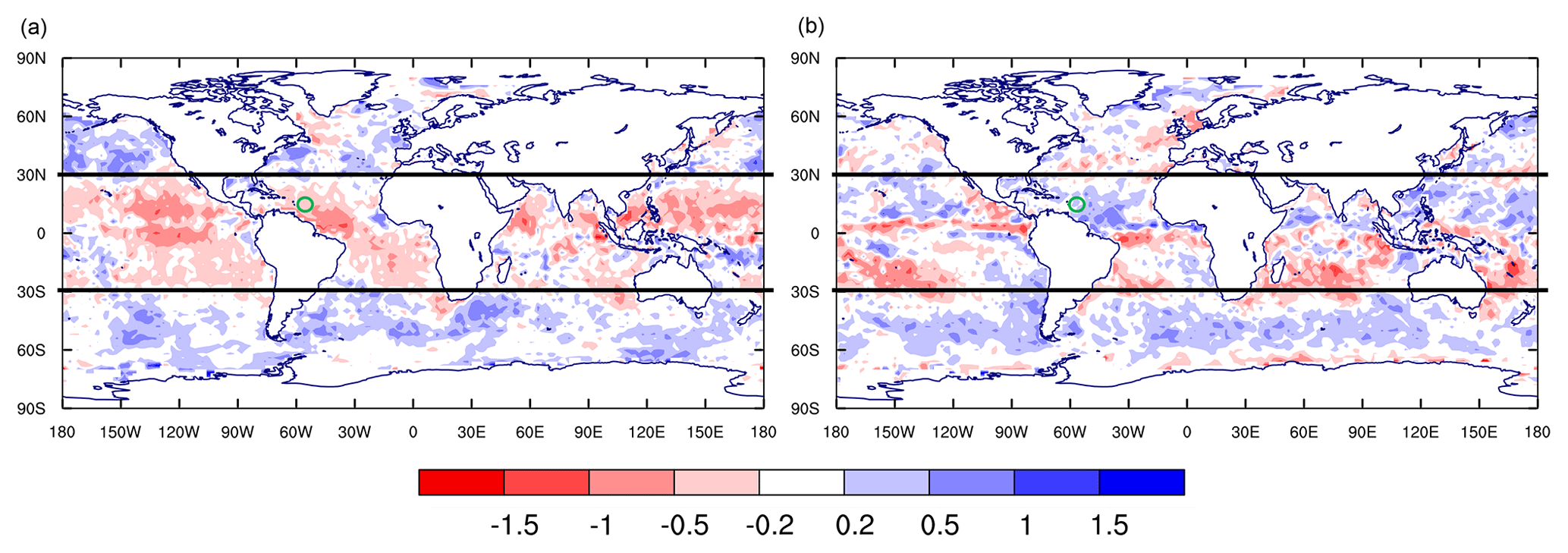
Figure 1 Surface wind bias with respect to ASCAT in the ECMWF operational deterministic forecasts for the months of January and February 2020. The green circles include the study area of EUREC⁴A. Panels (a) and (b) refer to the zonal and meridional wind components, respectively.

For the EUREC⁴A period we show (Fig. 1) global maps of the surface wind bias with respect to ASCAT as in Sandu et al. (2020). As already suggested by Sandu et al. (2020), the surface bias near Barbados is representative of the entire trade region, and during the campaign the bias is consistent with the average for the wintertime. On average, the zonal component is overestimated and the meridional component is underestimated.

Some aspects of the systematic error in surface winds from weather models have been described in the literature, for instance the insufficient mesoscale variability in the extratropics (Gille, 2005), the lack of small-scale features relevant for sea surface temperature (SST) gradient effects (Chelton et al., 2004; Risien and Chelton, 2008), and the generally excessive zonal winds (Chaudhuri et al., 2013; Belmonte Rivas and Stoffelen, 2019; Sandu et al., 2020). In the Northern Hemisphere there is a clear veering of the forecasted surface wind direction with respect to observations, leading to a smaller wind turning angle between the forecasted surface wind and the forecasted geostrophic wind than that seen in observations (Sandu et al., 2020).

In this study we focus on the representation of the vertical profile of winds during EUREC⁴A in operational forecasts and the ERA5 reanalyses produced with the ECMWF IFS. Our objectives are to

• a.

  combine various wind profiling observations to investigate the temporal variability of the wind bias in the operational ECMWF high-resolution deterministic short-range forecasts (approximately 9 km at the Equator),

• b.

  evaluate the differences in the bias of the analyses and reanalyses compared to the bias of the forecasts,

• c.

  assess the extent to which the assimilation of observations gathered during EUREC⁴A helped improve the analyses and forecasts performed with the IFS, and

• d.

  explore the origin of the wind bias through the use of additional model sensitivity experiments.

After a description of the data (Sect. 2) and the methods used to derive and compare statistics of the wind profiles (Sect. 3), we present a description of the observed wind profiles during EUREC⁴A (Sect. 4). In Sect. 5 we look at modeled winds and answer the following questions. What is the vertical distribution of the wind bias in forecasts and reanalyses produced with the IFS? How much are the analyses constrained by the assimilation of radiosondes and dropsondes during EUREC⁴A? What is the temporal variability of the wind bias? In Sect. 6 we then evaluate the influence of model physics, in particular the role of convection and turbulence representation. Our results are summarized and discussed in Sect. 7.

2 Data

Within EUREC⁴A, a region of intensive measurements was defined; it is situated in the trade-winds region near the western end of the “trade-wind alley”, which is an extended corridor across the Atlantic (see Fig. 1 in Stevens et al., 2021) with its downwind terminus defined by the Barbados Cloud Observatory (BCO). We adopt this region as the domain of our study (Fig. 2). More precisely, we cover an area of about 350 km × 350 km between 55.8 and 59.25^∘ W and between 11.4 and 14.7^∘ N. Our study samples 29 d during the boreal winter from 18 January 2020 to 15 February 2020. During the boreal winter the Intertropical Convergence Zone (ITCZ) is typically located at lower latitudes, and the area east of Barbados experiences undisturbed trade winds from an east to northeast direction, with the prevalence of cumulus clouds confined to the lower troposphere, moderate large-scale subsidence, and an inversion around 800 hPa (Stevens et al., 2016; Brueck et al., 2015; Nuijens et al., 2014).

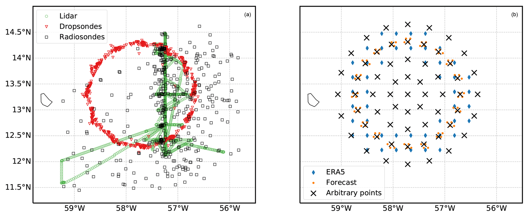
Figure 2 Overview of the spatial coverage of different datasets. Panel (a) illustrates the observational datasets: 3169 lidar measurements from the Meteor research vessel (green circles), 444 radiosondes from research vessels (black squares), and 799 dropsondes from JOANNE (red triangles). Panel (b) illustrates the points in which profiles were retrieved from IFS forecasts and (re)analyses. Model grid points are shown only for the second most external ring: see text for an explanation of different modeling datasets and resolutions.

Several observational datasets, such as dropsondes, radiosondes, and a shipborne wind-lidar system, are used to evaluate the forecasts and (re)analyses produced with ECMWF IFS.

2.1 Observations

2.1.1 JOANNE

We use EUREC⁴A dropsonde measurements from the JOANNE (Joint dropsonde Observations of the Atmosphere in tropical North atlaNtic meso-scale Environments) dataset (George et al., 2021a). Level 3 of this dataset is made available with a homogenized vertical resolution of 10 m. The primary strategy of the EUREC⁴A dropsonde launches was to sample atmospheric profiles along a ∼ 222 km diameter circle centered at 13.3^∘ N, 57.7^∘ W. Following Stevens et al. (2021), we call this the EUREC⁴A circle. The majority of the dropsondes over the EUREC⁴A circle were launched from the German high-altitude and long-range research aircraft HALO, with a few complementary flights also being performed by the American WP-3D Orion research aircraft. Typically, a flight over the EUREC⁴A circle took 1 h and 12 dropsondes were launched per circle, although the number of profiles per circle is often less than 12 due to either instrument or operator errors. An overview of the circles and corresponding dropsondes is outlined in George et al. (2021a). For our study, we use sounding profiles from 799 dropsondes (see red dots in Fig. 2) launched from 73 EUREC⁴A circles spread over 13 d between 18 January 2020 and 15 February 2020. In this study, we refer to the days with dropsonde measurements as flight days, and we use flight hours for the hours with dropsonde measurements within the flight days. We produce one mean dropsonde profile for each flight circle. Figure 3 schematically represents the temporal availability of JOANNE and of the other EUREC⁴A datasets used in this study. Black stripes indicate hours sampled in the corresponding dataset.

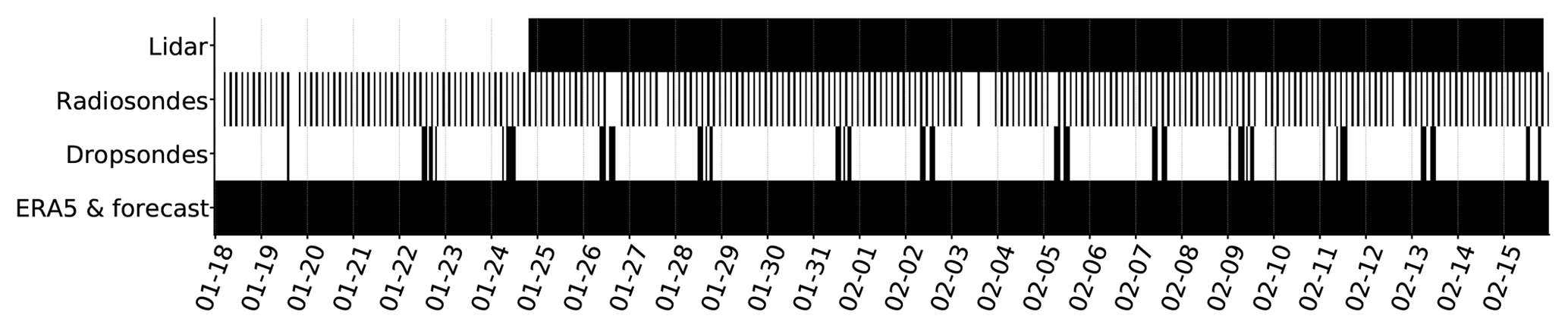
Figure 3 Overview of the temporal coverage of different observational datasets from EUREC⁴A which are used in this study. A black stripe indicates the availability of data for the corresponding hour.

2.1.2 Radiosondes

Radiosondes considered in this study were launched from four research vessels (RVs) over the northwestern tropical Atlantic eastward of Barbados: two German research vessels, Maria S. Merian (Merian) and Meteor; a French research vessel, L'Atalante (Atalante); and a United States research vessel, Ronald H. Brown (Ron Brown). The Meteor operated between 12.5 and 14.5^∘ N along the 57.25^∘ W meridian. The Ron Brown measured air masses along the trade-wind alley, while the Merian and Atalante vessels mainly sailed southward of Barbados (see Fig. 1 in Stevens et al., 2021). Most radiosondes recorded information in both the ascent and descent sections, with descending radiosondes falling by parachute for all platforms except for the Ron Brown.

This study makes use of 444 radiosondes (258 in ascending mode and 186 in descending mode) within the study domain defined above, as documented in Stephan et al. (2021). We use Level 2 of this dataset, which is made available with a vertical resolution of 10 m. Each black square in Fig. 2 (left) refers to a radiosonde either in ascending or descending mode. Radiosondes drifting outside the area of interest are considered only when inside the domain, and radiosondes launched outside and drifting inside the domain are also considered only where relevant.

There are about two radiosondes per hour, and we produce one averaged wind profile every 3 h to represent the entire domain. The radiosondes provide a regular and comprehensive dataset during all days of the study, as can be seen in Fig. 3.

2.1.3 WindCube long-range wind lidar

A Leosphere long-range WindCube (WLS70) on board the Meteor research vessel performed measurements at 20 different height levels every 100 m between 100 and 2000 m. The WLS70 device has a sampling rate of approximately 6 s and measures the line-of-sight radial velocity successively at four azimuthal positions along a cone angle of 14.7^∘; thus, every 360^∘ scan takes around 24 s.

The radial velocities are corrected for ship motions with a simplified correction methodology using an internal GPS system of an accompanying short-range WLS7 WindCube, which uses a combination of an xSEns MTi-G attitude with heading reference sensor (AHRS) and a Trimble SPS361 satellite compass. The simple motion correction applied to the line of sight (LOS) velocities takes into account the translational ship motions and the yaw information, as explained in Wolken-Möhlmann et al. (2014) and Gottschall et al. (2018). The pitch and roll information is not used, since according to previous studies (Wolken-Möhlmann et al., 2014), the effects of these tilt motions are less relevant for relatively stable platforms. After corrections, the wind vector is retrieved and the data are averaged to 1-hourly values.

The left panel of Fig. 2 shows the location of the RV Meteor carrying the WindCube every 10 min (in green). Figure 3 shows that wind profiles from lidar measurements are available continuously from 25 January to 15 February.

2.2 Modeling datasets

The modeling datasets comprise the operational (at the time of the campaign) deterministic high-resolution (9 km) forecasts, the ERA5 reanalysis (Hersbach et al., 2020), and several experiments at coarser resolution. The modeling data are on hybrid vertical coordinates, which give about 20 m resolution near the surface and ∼ 300 m resolution at 5 km. For each of these datasets, model output was extracted at the nearest four neighbors of 61 points placed concentrically around the center of the EUREC⁴A circle. Each group of four points was then used to interpolate the model values to the locations of the 61 arbitrary points using an inverse distance weighting method. This method is applied to reduce to a minimum the already marginal impact of different spatial resolutions on the results of this study. The location of these 61 arbitrary points is shown in the right panel of Fig. 2 with black crosses. They are chosen to represent the mean state of the study area, with particular attention to the EUREC⁴A circle, which coincides with the second most external ring of points.

2.2.1 Forecast

For the operational ECMWF deterministic 10 d forecasts (cycle 47r2) the extracted model grid points for the EUREC⁴A circle are marked in orange in Fig. 2b. For clarity, we avoid showing the rest of the extracted model grid points. We extract hourly output for day 2 of the forecasts (lead time of 24 to 48 h) and hereafter we will refer to this simply as forecast. We focus on these short-range forecasts after Sandu et al. (2020) showed that over this trade-winds region the errors in wind profiles develop in the first 12 h of the forecast and do not grow significantly until day 5.

2.2.2 ERA5

The fifth generation ECMWF global reanalysis (ERA5) produced for the Copernicus Climate Change Service is widely used for model evaluation, and often it is used as a proxy for observations. Similar to the operational analysis, ERA5 is produced with ECMWF IFS by optimally combining short-range forecasts and observations through data assimilation (as is done to create the analysis or initial condition of the forecasts). While operational analyses are not consistent in time because of regular upgrades to the forecasting system, reanalyses are produced with a unique version of the forecasting system. This leads to a consistent time series, which allows one to monitor environmental changes. ERA5 is produced with the IFS model cycle 41r2 at a resolution of approximately 32 km and covers the period 1950 to present (Hersbach et al., 2020).

Here we exploit EUREC⁴A observations to also evaluate the quality of the wind profiles in the ERA5 reanalysis. The extraction points for ERA5 corresponding to the EUREC⁴A circle are shown in blue in Fig. 2b. In the sections below we focus on the wind profiles from ERA5, rather than from the operational analysis, because the differences in wind profiles over the EUREC⁴A region between the operational analysis and ERA5 are marginal (not shown) but ERA5 is available hourly, whereas the operational analysis is available 6-hourly. The choice of using ERA5 is also motivated by its widespread use in the literature as a reference and truth.

2.2.3 Sensitivity experiments

EUREC⁴A dropsondes and radiosondes are assimilated in ERA5, which may lead to an underestimation of the bias calculated with respect to these measurements. Sentić et al. (2022) recently analyzed the impact of dropsondes on the ECMWF IFS analysis and found overall small differences. For our case, we similarly investigate to what extent the IFS reanalysis is close to reality because local observations are assimilated. To answer this question, several sensitivity experiments were performed at 40 km resolution with outputs saved every 3 h for the forecasts and every 6 h for the analyses.

First, a control analysis (CTRL_an) and corresponding 10 d control forecasts (CTRL_fc) initialized from it were performed at this resolution. Second, so-called data denial experiments were performed in which measurements made during EUREC⁴A are not assimilated when creating the initial conditions of the forecasts. These experiments consist of (a) an analysis experiment in which the EUREC⁴A dropsondes are not assimilated as well as corresponding 10 d forecasts (Exp1_an, Exp1_fc) and (b) an analysis experiment wherein neither EUREC⁴A dropsondes nor radiosondes are assimilated as well as corresponding 10 d forecasts (Exp2_an, Exp2_fc).

Another pair of experiments allow us to explore the origin of the IFS wind bias. We performed an analysis experiment and corresponding 10 d forecasts, for which shallow convective momentum transport is switched off (Exp3_an, Exp3_fc). In the IFS cumulus convection is parameterized with a bulk mass-flux scheme, which was originally described in Tiedtke (1989). Clouds are represented by a single pair of entraining–detraining plumes, which describes updraft and downdraft processes. Convection is classified as shallow when the cloud top is below 200 hPa and deep otherwise. This distinction is only necessary for the closure and the specification of the entrainment rates that are a factor of 2 larger for shallow convection (IFS, 2020).

Lastly, an experiment is performed with the most recent IFS cycle (47r3), which was not yet operational at the time of the campaign. This is used to investigate the role of the model physics in determining the wind bias, particularly the deep convection away from Barbados. For all the abovementioned sensitivity experiments forecasts were initialized daily at 00:00 UTC from the corresponding analysis.

3 Methods

Mean wind profiles are derived using the datasets described above. The differences between the modeled and observed winds are quantified by computing the instantaneous model error (Θ_mod−Θ_obs) at all time stamps and subsequently defining the mean model bias and the root mean square error (RMSE) as

$$\begin{array}{}\text{(1)}& {\displaystyle }\mathrm{Bias}=\stackrel{\mathrm{‾}}{{\mathrm{\Theta }}_{\mathrm{mod}}-{\mathrm{\Theta }}_{\mathrm{obs}}},\text{(2)}& {\displaystyle }\mathrm{RMSE}=\sqrt{\stackrel{\mathrm{‾}}{{\left({\mathrm{\Theta }}_{\mathrm{mod}}-{\mathrm{\Theta }}_{\mathrm{obs}}\right)}^{\mathrm{2}}}},\end{array}$$

where the overbar represents the arithmetic mean and Θ is any modeled (mod) or observed (obs) variable.

While the RMSE measures model accuracy independent of the sign of the error, the model bias takes into account the sign of the errors and can be used to study the distribution of the error. The skewness of the error distribution is important for the bias: large errors that are normally distributed result in large values of RMSE but a bias that is approximately zero. Otherwise, said positive and negative errors can compensate for each other and result in a nearly zero mean bias.

All profiles are interpolated to a grid of 50 m vertical resolution between 0.15 and 5 km for simplicity. The mean sub-cloud layer top (630 m) and the mean inversion height (2260 m) are calculated from the JOANNE dataset. The sub-cloud layer top is defined as the height at which relative humidity maximizes below 1 km. The inversion height is defined as the altitude below 6 km at which the Brunt–Väisälä frequency squared (N²) is maximum. The wind vectors are decomposed into zonal (u) and meridional (v) components and analyzed at different hours of the day using hourly and 3-hourly composites. While the modeling datasets directly provide vectorial wind components, the observations measure scalar quantities such as wind speed (wspd) and wind direction. In this study we retrieve the corresponding meridional and zonal components for each radiosonde and dropsonde as well as for each of the 10 min lidar winds, thus before computing any mean.

While model outputs uniformly sample the entire domain at each time step, observations only sample one location at the time. To partially account for these differences in the datasets, we sample the model output to match the sampling of the respective observational dataset when we derive the forecast and (re)analysis errors. For example, when we compare to the radiosondes, we average the model profiles for the 61 points and over 3-hourly intervals, assuming that the launch locations over 3 h are sufficiently dispersed to provide a good representation of the entire domain. When we compare to the dropsondes, we average only the model points extracted along the EUREC⁴A circle at the hour during which the circle was flown. In the case of the wind lidar, we use only the closest extraction point to the instrument when computing the model errors. When the model is simultaneously compared to multiple observational datasets (e.g., in Figs. 5a–c and 7a–c), we show the model mean obtained from all 61 points and with the temporal resolution available for the model output.

Figure 4 Spatial variability of wind components (zonal u, meridional v, and wind speed – wspd) at 500 m derived from ERA5 for the whole period and at all hours.

Figure 4 helps quantify the spatial variability of winds in the study area and motivates our choice of the spatial matching between observations and the model output. It shows that there is a NW to SE gradient in wind, whereby the southeast region of the domain experiences winds about 0.5 m s⁻¹ stronger than the average of the domain. The lidar samples this region more frequently than the northwest area where weaker winds prevail. Thus, we expect the wind-lidar winds to generally be stronger.

4 Observed winds during EUREC⁴A

4.1 Wind profile and synoptic variability

EUREC⁴A was characterized on average by low-level northeasterly winds, as shown in Fig. 5a and b, which includes both observations (radiosondes in black and lidar in green) and models (in blue). The JOANNE dropsonde dataset is not shown because of the limited number of flight days and because JOANNE does not sample all hours of the day. We will show in Sect. 5.3 that on flight hours dropsondes and radiosondes only disagree for the zonal component in the cloud layer (630–2260 m). Note that the lidar measured stronger winds in the sub-cloud layer while deployed in a region where winds were stronger (Sect. 3).

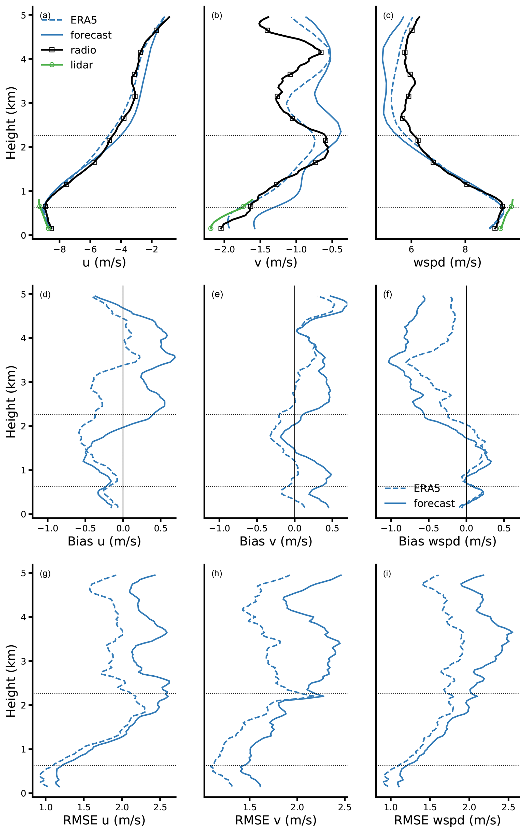
Figure 5 Mean profiles of zonal wind (a, d, g), meridional wind (b, e, h), and wind speed (c, f, i) during EUREC⁴A. In the top row (a–c) are monthly profiles retrieved from lidar (green circles), radiosondes (black squares), ERA5 reanalysis (dashed blue), and day 2 forecast (solid blue). The middle (d–f) and bottom (g–i) rows show the monthly biases and root mean square error of the forecast and ERA5 with respect to radiosondes. The horizontal dotted lines indicate the mean sub-cloud layer top and inversion height.

The mean wind speed (Fig. 5c) is about 9 m s⁻¹ at 150 m; it slightly increases in the lower 800 m and is sharply reduced to 6 m s⁻¹ in the cloud layer between 1 and 2 km. The zonal component is the largest contributor to the total wind speed, which typically peaks near cloud base and decreases aloft, establishing a so-called backward sheared wind profile. This structure was documented in earlier field studies (Riehl et al., 1951; Brümmer et al., 1974) and more recently using the BCO climatology alongside ERA-Interim (Brueck et al., 2015). A recent study using North Atlantic large eddy simulations with ICON (hindcasts performed for the pre-EUREC⁴A NARVAL campaign period) suggests that the local maximum in zonal wind near cloud base results from efficient turbulent diffusion in the sub-cloud layer but little if any cumulus friction at cloud base (Helfer et al., 2021). In the cloud layer counter-gradient momentum transport is found, which suggests that moist convection tends to enhance and not reduce the vertical wind shear above ≈ 1 km (Larson et al., 2019; Dixit et al., 2021).

The mean meridional wind maximizes closer to the surface with wind speeds of about −2 m s⁻¹, and it decreases in magnitude (negative numbers) to −0.5 m s⁻¹ at 2 km.

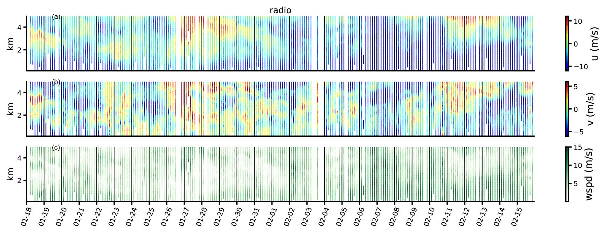
Figure 6 Time series of 3-hourly zonal wind (a), meridional wind (b), and wind speed (c) from radiosondes averaged over the whole domain.

Although the trade winds are generally steadier than midlatitude flows, they still exhibit significant synoptic variability. Figure 6 shows the observed winds (zonal and meridional wind as well as wind speed) at 3-hourly resolution derived from the radiosondes. Winds were relatively weak with strong backward shear during the final 2 weeks of January 2020, transitioning to a period with stronger winds and weaker shear during the first week of February 2020, and the campaign ended with several days with strong winds and strong backward shear.

4.2 Wind diurnality

An important highlight of EUREC⁴A, although not novel, is the presence of pronounced diurnality in both convection and the winds. Figure 7a–c plot hourly and 3-hourly wind composites averaged over the layer between 0.15 and 0.75 km from the lidar data (green) and the radiosondes (black). A diurnal cycle is present, with the weakest wind speeds during the day and the strongest winds at night. The amplitude of the observed diurnal cycle is about 1 m s⁻¹ in both the meridional and zonal component.

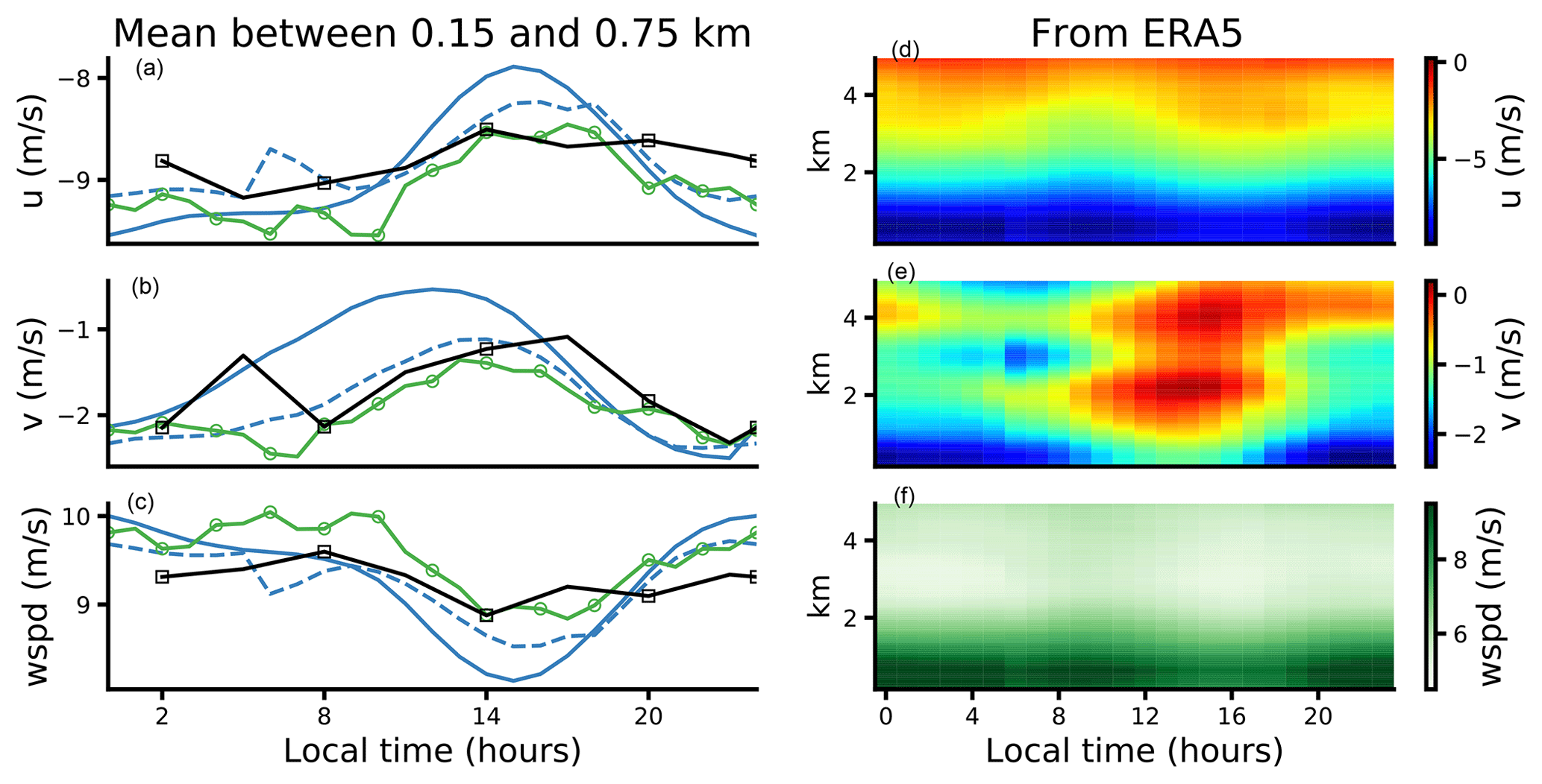
Figure 7 Diurnal cycle of zonal wind (a, d), meridional wind (b, e), and wind speed (c, f). The left column (a–c) refers to the layer between 0.15 and 0.75 km with values from radiosondes (black squares), lidar (green circles), ERA5 (dashed blue), and the forecast (solid blue). The right column (d–f) refers to multiple levels from the surface to 5 km with values from ERA5 only.

The diurnal wind variations are not fully understood, but Ueyama and Deser (2008) showed that over the tropical Pacific such variations agree very well with pressure-derived wind diurnality, suggesting that the pressure gradient force plays a dominant role in setting the diurnality, next to a possible role for boundary layer stability and/or diurnality in moist convection. We will return to this in Sect. 6, where we present the diurnality in the large-scale pressure gradient as part of the observed and modeled momentum budget.

5 Modeled winds

5.1 Mean bias

The EUREC⁴A mean zonal wind profile in Fig. 5 is captured well by ERA5 (blue dashed line) and the forecast (solid blue line), particularly below 2 km, but the forecast especially suggests weaker meridional winds at all heights, in particular near 0.15 and 3 km. A bias in the wind direction, with winds veered with respect to the observations, has long been known to be present in the model; see also Sandu et al. (2020) and the comparison of ERA5 and surface scatterometer winds in Belmonte Rivas and Stoffelen (2019). Less appreciated is that the wind bias (see also the actual bias with respect to the radiosondes in Fig. 5d–f) is larger above the boundary layer, while it is small (∼ 0.1 m s⁻¹) below roughly 2 km (near the trade inversion).

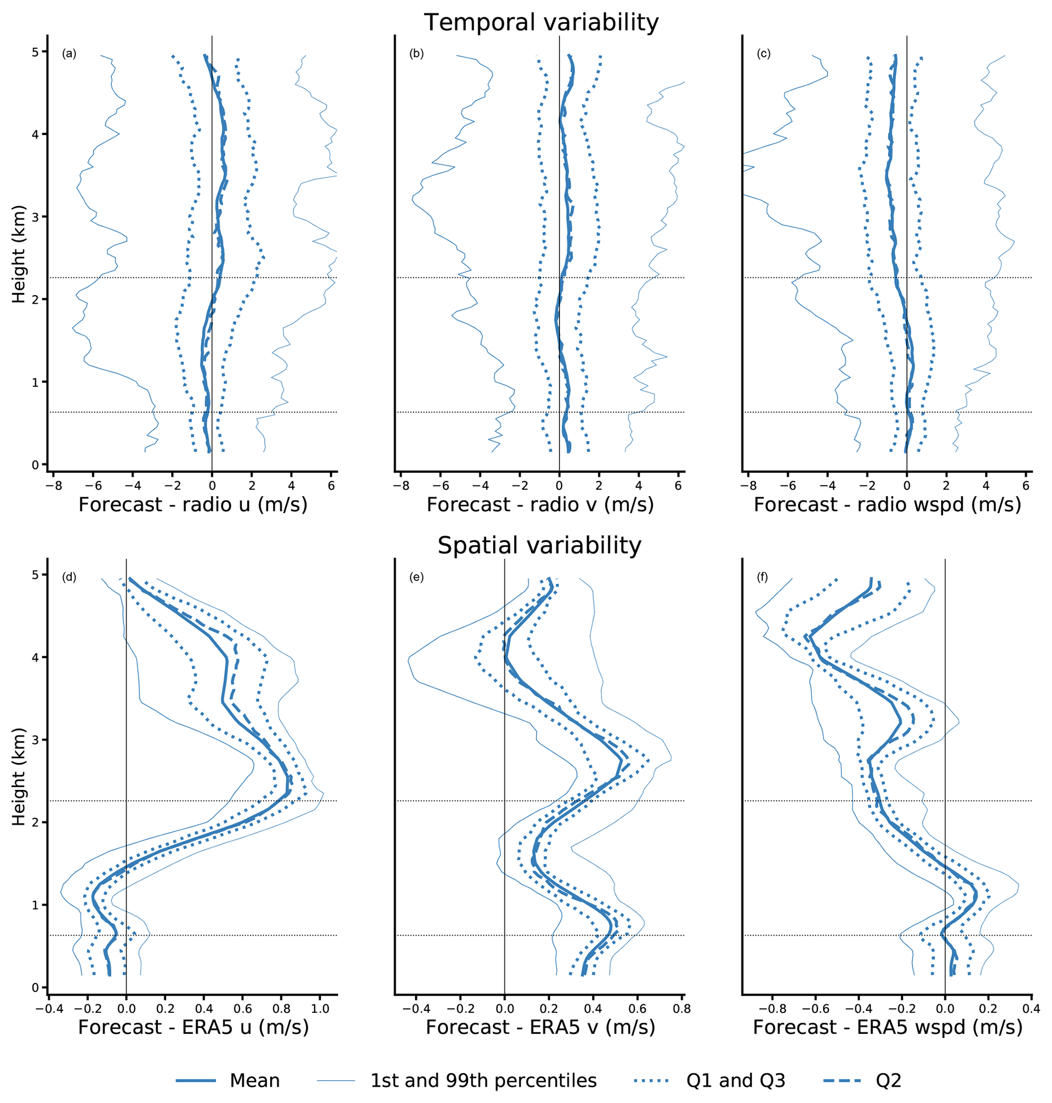
Figure 8 Statistical distribution over time of the forecast error with respect to the radiosondes for all levels up to 5 km (a–c). Statistical spatial distribution for the 61 extraction points of the difference between the forecast and ERA5 (d–f).

However, the mean bias is not a good representation of the errors made on shorter timescales. Figure 5g, h, and i show that the RMSE between the forecast–ERA5 and radiosondes is as large as 1 m s⁻¹ at 250 m and 2.5 m s⁻¹ between 3 and 4 km for all components. Figure 8 shows – as a function of height – the mean, the quartiles (Q1, Q2, Q3), and the first to last percentiles of the forecast errors at individual times (top row). The interquartile range of errors can be up to ±1 m s⁻¹, while the first and last percentiles range ±4 m s⁻¹. The errors are fairly normally distributed, and as such the mean bias can be small.

With the data available here, the spatial distribution of the model bias can only be addressed with dropsondes on the HALO circle and thus for a few days. Instead, we show the difference between the forecast and ERA5 for all 61 extraction points and investigate the spatial variability of this difference for the entire period (Fig. 8d–f). Compared to the temporal variability, the errors made at individual locations within the circle are far more similar and at least an order of magnitude smaller, ranging ±0.4 m s⁻¹.

As expected, the bias and RSME of ERA5 are smaller than those of the forecast. The radiosondes and dropsondes launched during EUREC⁴A were used in the data assimilation process of ERA5. The following section investigates to what extent the assimilation of these observations has influenced the performance of the analysis and the forecast.

5.2 Influence of sounding assimilation

We performed extractions from the IFS analysis and forecast of a control experiment (CTRL_an, CTRL_fc), an experiment without assimilating dropsondes (Exp1_an, Exp1_fc), and an experiment without assimilating dropsondes nor radiosondes (Exp2_an, Exp2_fc). For each of the mentioned experiments the monthly mean bias and RMSE are calculated over all hours of the day with respect to the radiosondes, as done in Fig. 5d–i. The results are shown in Fig. 9, where the dashed lines refer to the analyses and the solid lines to the forecasts.

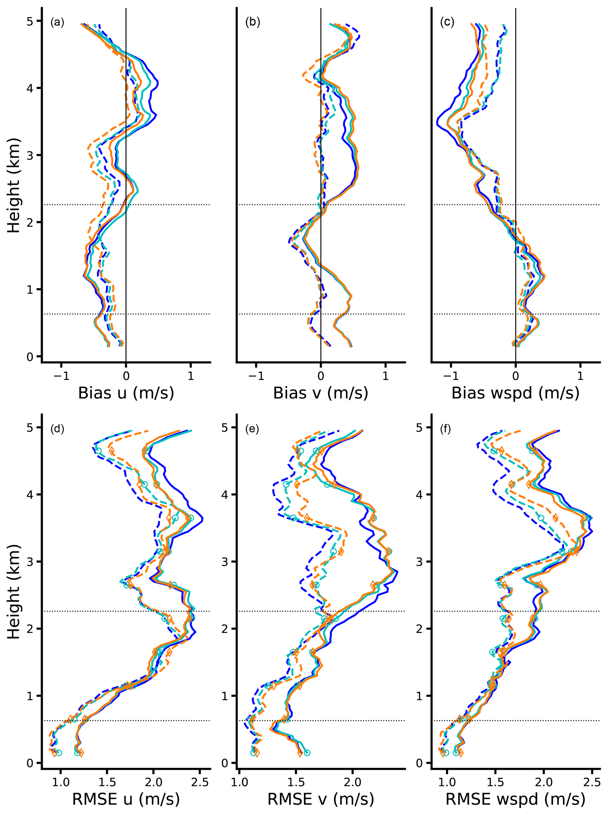
Figure 9 Monthly mean IFS bias (a–c) and root mean square error (d–f) against radiosondes as in Fig. 5d–i; forecasts are in solid and analyses in dashed. In the control experiment (blue) both dropsondes and radiosondes from EUREC⁴A are assimilated. In the first experiment (cyan) dropsondes are excluded from the assimilation. In the second experiment (orange) neither dropsondes nor radiosondes are assimilated.

Evidently, all analysis and forecast experiments remain considerably close to the corresponding control experiment (blue lines): the differences are small everywhere and almost nonexistent below 2 km. The sign, shape, and magnitude of the profiles in Fig. 9 confirm the results described in previous sections (see, e.g., Fig. 5) and support the idea that the mean wind bias does not increase with coarser model runs (40 km spatial resolution and 3 h temporal resolution of the model output). This also suggests that assimilating the local soundings does not alleviate the existing biases.

That the analyzed wind profile error does not change much in any of the denial experiments does not necessarily mean that the observations have not played a role in constraining the wind profiles, because typically, when one observing system is withdrawn from the data assimilation system, the analysis is constrained through other observing systems (Sandu et al., 2020).

The variability in the (sign of) errors is explored next and also shown to critically depend on the time of the day.

5.3 Temporal structure of the bias

Do certain days during EUREC⁴A have systematically larger wind errors? The sign and magnitude of the 3-hourly biases (Fig. 10) are relatively similar in the first and second half of the EUREC⁴A period, with positive and negative values of up to 2 m s⁻¹ in both the zonal and the meridional wind components that sometimes last just a few hours and sometimes several days. The 3-hourly forecast bias with respect to radiosondes shows a similar results but with larger values (not shown).

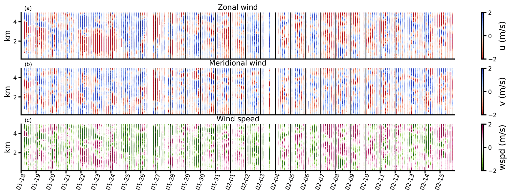
Figure 10 Difference between ERA5 and radiosonde wind profiles averaged over the whole domain and over 3-hourly intervals. From top to bottom: zonal winds, meridional winds, and wind speed.​​​​​​​

A more systematic bias is seen in the diurnal cycle of winds, which was already hinted at in Fig. 7. The wind diurnality is significantly overestimated by the forecast with an amplitude almost twice that of the observations. At 15:00 LT the zonal wind bias is largest: the forecast underestimates the magnitude of the zonal wind component by 1 m s⁻¹ with respect to both lidar and radiosonde measurements. Instead, in the late night and early morning the forecast biases are most pronounced in the meridional wind (Fig. 7b): the forecast is out of phase, exaggerating and anticipating the morning weakening of the meridional wind.

ERA5 is notably better at capturing the amplitude and phase of the diurnal cycle in the meridional component, despite the fact that the assimilation of local dropsondes and radiosondes is not important for reducing the bias (Sect. 5.2). The origin of the diurnality in winds is not fully understood. Above 2 km, the zonal and total wind speed variations (Fig. 7d–f) suggest a semi-diurnal cycle of the zonal winds, with weakest winds in the first few hours of the day and around 16:00 LT. Such a semi-diurnal cycle in zonal winds (and diurnal cycle in meridional winds) has been found over the tropical oceans in earlier studies (Dai and Deser, 1999; Ueyama and Deser, 2008) and linked to semi-diurnal atmospheric thermal tides generated by the absorption of solar radiation by ozone in the stratosphere and water vapor in the troposphere. These tides travel downward and affect sea level pressure, whose tidal amplitudes appear mostly semi-diurnal.

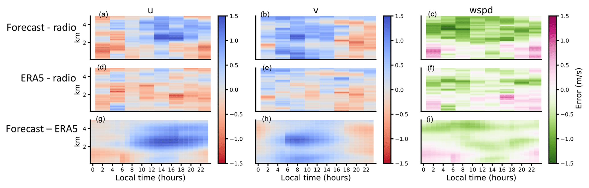
Figure 11 Diurnal cycle of the forecast bias with respect to radiosondes (a–c), the ERA5 bias with respect to radiosondes (d–f), and the forecast bias with respect to ERA5 (g–i). From left to right, columns refer to the biases in zonal wind, meridional wind, and wind speed. Blue regions are related to a positive bias (e.g., negative zonal wind that is too weak), and red regions are related to a negative bias (e.g., wind speed that is too weak).

Figure 11 quantifies the mean model bias as a function of height and time of day with respect to radiosondes (Fig. 11a–c and d–f), while Fig. 12 shows the mean bias during flight hours (Fig. 12a–c), daytime (between 10:00 and 16:00 LT), and nighttime (between 22:00 and 04:00 LT). These figures reveal that an overly strong easterly wind in the IFS during nighttime (as found near the surface in Fig. 7) is present throughout the lower 2 km of the atmosphere. During daytime and during flight hours (which are predominantly during daytime), the meridional wind component contributes most to the weak wind speed bias in the forecasts below 2 km. Overly weak easterly wind are seen also above 2 km, where both meridional and zonal winds are underestimated (Figs. 11 and 12).

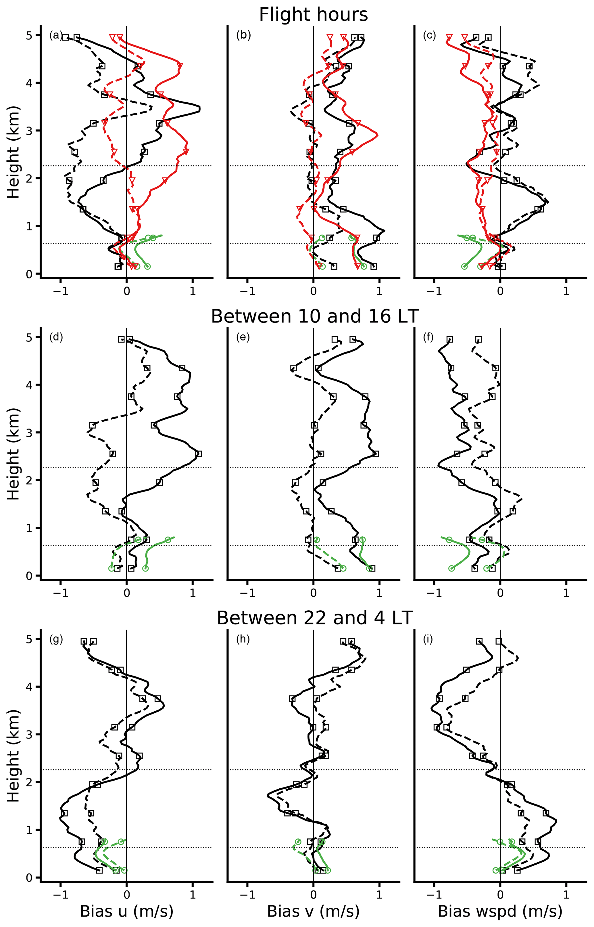
Figure 12 Mean model bias (forecast in solid and ERA5 in dashed) during flight hours (a–c) and during the whole EUREC⁴A campaign, measured separately for daytime between 10:00 and 16:00 LT (d–f) and for nighttime between 22:00 and 04:00 LT (g–i). The bias is calculated with respect to radiosondes (black squares), lidar measurements (green circles), and dropsondes (red triangles). From left to right the columns refer to the bias in the zonal wind (u), meridional wind (v), and wind speed.

ERA5 performs much better than the forecast at all hours of the day. Nevertheless, the pattern in the rightmost panels (wind speed) suggests that the reanalysis only reduces the magnitude of the bias, without eliminating the fundamental causes of an overestimated diurnal wind cycle below 1 km. At nighttime the forecast is close to ERA5, while during daytime the forecast and ERA5 differ considerably (more than 1 m s⁻¹ at 2.5 km for both the zonal and meridional components). This can be traced back to what is seen in Fig. 7, where both the forecast and reanalysis overestimate the amplitude of the diurnal cycle, but only ERA5 captures the phase of the cycle.

From Fig. 12a–c we can also infer that the dropsondes and radiosondes agree fairly well, apart from the zonal wind in the cloud layer. Here, at about 1.5 km, the radiosondes show zonal winds ∼ 1 m s⁻¹ stronger than the dropsondes. These differences may be due to differences between the descending and ascending radiosondes. Descending radiosondes tend to show stronger winds above 1.5 km. Excluding the 186 descending radiosondes produces better agreement with the dropsondes above 2 km (not shown). However, around 1 km the descending radiosondes match the dropsondes considerably better than the ascending radiosondes. We also notice that the number of operating dropsondes is reduced at lower altitudes.

6 The role of parameterized moist convection

Previous sections highlighted that a wind speed bias exists throughout the lower troposphere and not just near the surface. To address the role of shallow moist convection in setting the bias, this section compares the modeled momentum budget with the observed momentum budget during EUREC⁴A and discusses a sensitivity experiment that removes momentum transport by shallow convection, which already has a profound effect on the circulation. Rather than turning off shallow convection entirely, which would lead to a substantially different structure of the trade-wind layer, the control run can be compared to the latest IFS model cycle 47r3, which has a different representation of moist physics.

6.1 Observed versus modeled momentum budget

In Fig. 13 the mean tendencies in the momentum budget are compared against the mean momentum tendencies derived from the JOANNE dataset (Sect. 2.1.1). Figure 13a and b represent the average over all flight hours during all flight days, while the daytime and nighttime tendencies over all EUREC⁴A days and just for the model are shown in Fig. 13c and d as well as Fig. 13e and f. In the observations (solid lines) and in the IFS (dashed lines), the advection, pressure gradient, and Coriolis force are combined into a “dynamical” forcing that acts on the scale of the circle (∼ 200 km). In the model, the so-called “frictional force” is comprised of parameterized convective and turbulent momentum transport. In the observations, it is derived as the residual in the momentum budget and interpreted as the vertical eddy flux divergence established by turbulent flows within the circle (including small-scale turbulence, convection, and mesoscale circulations) (Nuijens et al., 2022). Horizontal advection and vertical advection of the mean wind are combined and on average an order of magnitude smaller than the other budget terms (not shown), so the momentum balance is predominantly a balance between the pressure gradient force, a Coriolis force, and friction.

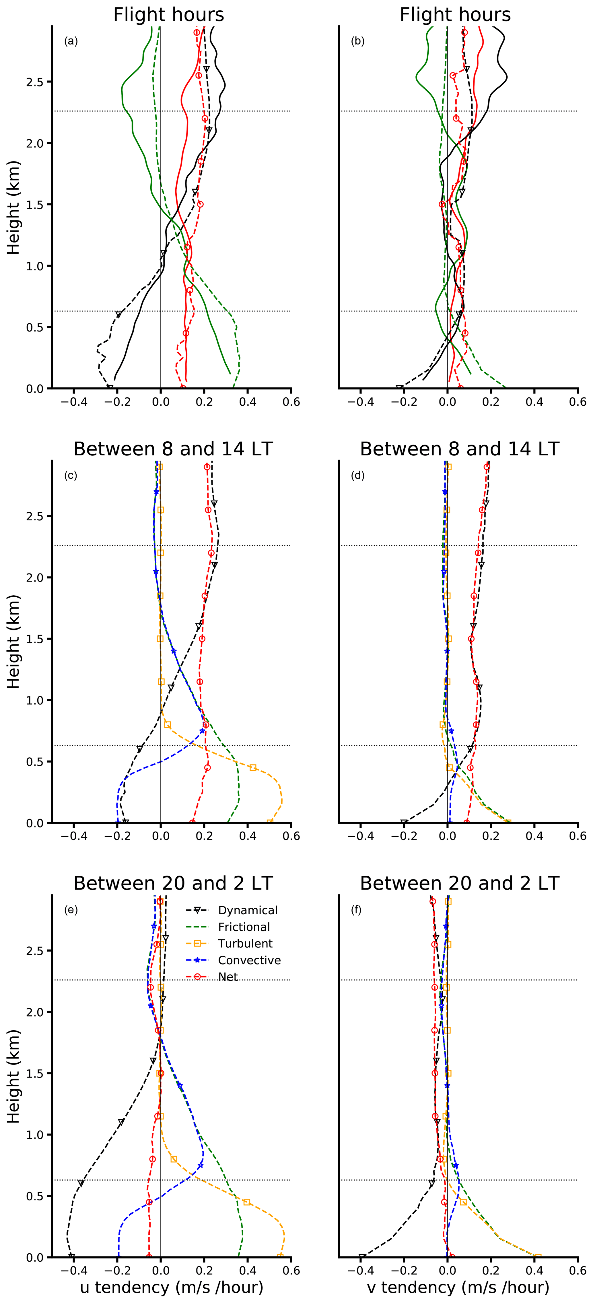
Figure 13 Components of the momentum budget retrieved from the dropsondes (solid) and the forecast (dashed). The net tendency (red circles) balances the dynamical force (black triangles) and the frictional force (green). The latter is split into turbulent and convective for the forecast. The top row (a, b) refers to days and hours sampled by the dropsondes (flight hours). The middle row (c, d) refers to the hours between 08:00 and 14:00 LT during all EUREC⁴A days. The bottom row (e, f) refers to the hours 20:00 to 02:00 LT during all EUREC⁴A days.

Because most flight hours took place in the early morning, the observed and modeled tendencies are most comparable to the daytime tendencies between 08:00 and 14:00 LT (Fig. 13c, d). During this time the dynamical forcing is about half that of the forcing experienced at night (Fig. 13e, f). This diurnality in pressure gradients is not fully understood but may be linked to a diurnality in remote deep convection; e.g., deep convection in the ITCZ peaks in the early morning, while deep convection over the South American continent peaks in the afternoon (Wood et al., 2009).

There is remarkable agreement between the general structure and magnitude of the tendencies in the observations and the IFS in the boundary layer, providing confidence in the method used to estimate the budget from observations, as well as in the ability of the IFS to reproduce the different processes at play. There is a non-negligible positive net tendency in the zonal direction (red), in agreement with a slowdown of the easterly wind in the morning and afternoon, which is preceded by a reduction in the large-scale dynamical forcing (black lines in Fig. 13c and e).

Compared to the observations, the IFS has larger dynamical and frictional tendencies in the zonal component in the sub-cloud layer up to ∼ 0.75 km (Fig. 13a), where the observations suggest a gradual weakening of these tendencies with height. Because the turbulent friction and large-scale pressure gradients are coupled through the circulation, it is hard to disentangle which error is driving which. In the meridional component the model and observations agree on the dynamical forcing driving northerly winds below 500 m, but the IFS overestimates the frictional force.

Between 1.5 and 3 km the frictional force is near zero in the IFS, but the observations suggest a layer with negative frictional force (i.e., an acceleration of the easterly flow) that is near cumulus tops. As such there is a larger net deceleration of easterly winds in the IFS, consistent with the finding that the IFS has a slow zonal wind bias at those heights during flight hours (Fig. 12, top row). In the meridional component, the IFS appears to overestimate friction in the sub-cloud layer and underestimate friction above ∼ 500 m, where the observations suggest that small frictional effects are present (between 1 and 2 km). An acceleration of northerly winds in the observations is seen above 2 km.

6.2 Shallow convective momentum transport

In previous work, convectively driven circulations and variability have been suggested to play a role in the long-standing near-surface wind bias over subtropical oceans (Belmonte Rivas and Stoffelen, 2019; Sandu et al., 2020). We cannot disentangle the role of convection versus turbulence in the observed tendencies and therefore cannot test whether the IFS has either too little or too much (cumulus) friction at different levels (the abovementioned simulations target these open questions).

However, in the IFS we can turn off shallow convective momentum transport (CMT) to study which aspects of the wind bias are sensitive to the process. CMT acts to mix winds between the surface and the cloud layer. If the wind speed increases with height, as is typically true for the sub-cloud layer, this would result in an increase in wind speed near the surface and a decrease in wind speed in the cloud layer, the latter being the so-called “cumulus friction” effect. Without shallow CMT, the sub-cloud layer shear is expected to be enhanced. Figure 14 compares simulations without shallow CMT – Exp3_an and Exp3_fc in black dashed and solid lines with circles – to the same control experiment as in Sect. 5.2 (CTRL_an and CTRL_fc in dashed and solid blue). It confirms that shallow CMT acts to strengthen winds near the surface and weaken easterly winds in the cloud layer. Without shallow CMT, the bias near the surface disappears, but the bias around 1 km gets much larger. At this level, especially at night, overly strong easterly winds develop (Fig. 14d–f). This highlights the role of shallow convection in partially communicating wind biases from the lower cloud layer to the surface.

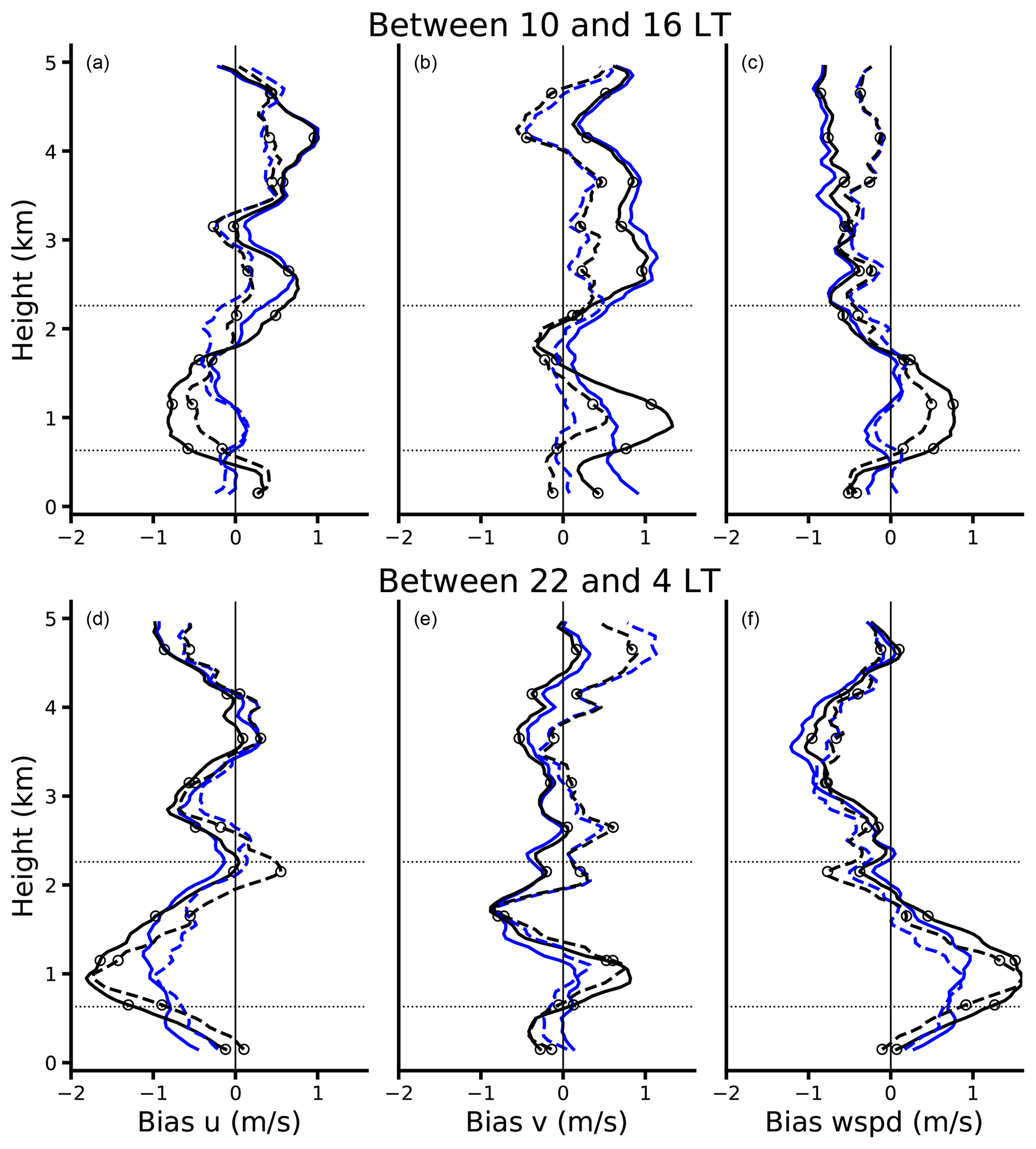
Figure 14 Mean IFS bias (forecast in solid and analysis in dashed) during EUREC⁴A with respect to radiosondes. Blue refers to the control experiment, while black circles refer to the experiment with convective momentum transport turned off (Exp3). The top (a–c) and bottom rows (d–f) respectively show the bias between 10:00 and 16:00 LT and between 22:00 and 04:00 LT.

Above 2 km, there is little difference between the black lines (Exp3_an and Exp3_fc) and the blue lines (CTRL_an and CTRL_fc) (Fig. 14). At these height levels, convective tendencies in the IFS are small or negligible (Fig. 13c–f), and the weak wind speed bias evident in both the zonal and meridional components remains.

6.3 New moist physics

In this section we compare a model experiment with the most recent IFS cycle (47r3) (Becker et al., 2021) to the forecast of cycle 47r2 used here, which was operational at the time of the field campaign. In the 47r3 cycle the main revisions concern the parameterization of deep convection, especially the representation of propagating mesoscale convective systems and their diurnal cycle (Bechtold et al., 2020). The coupling between convection and dynamics is improved by adding a tendency from the dynamics to the mass flux closure, namely the total (vertical and horizontal) advective moisture tendency. Insufficient nighttime convection over land has been identified as a major shortcoming in IFS forecasts of convective activity (Becker et al., 2021). Comparing the two cycles thus reflects changes in the wind bias that are more likely to be caused by changes in remote convection and subsequent changes in circulation patterns than by changes in local convection.

The red lines in Fig. 15 indicate that the mean wind bias with respect to radiosondes is largely reduced during daytime and above 2 km. The solid blue lines refer to the operational forecast, while the dashed blue lines refer to ERA5. We present separate panels for the EUREC⁴A mean over all hours of the day (Fig. 15a–c), for daytime (Fig. 15d–f), and for nighttime (Fig. 15g–i). The upgraded model improves the wind forecast everywhere except for a slight deterioration of the zonal component below 1.5 km during daytime and above 2 km during nighttime.

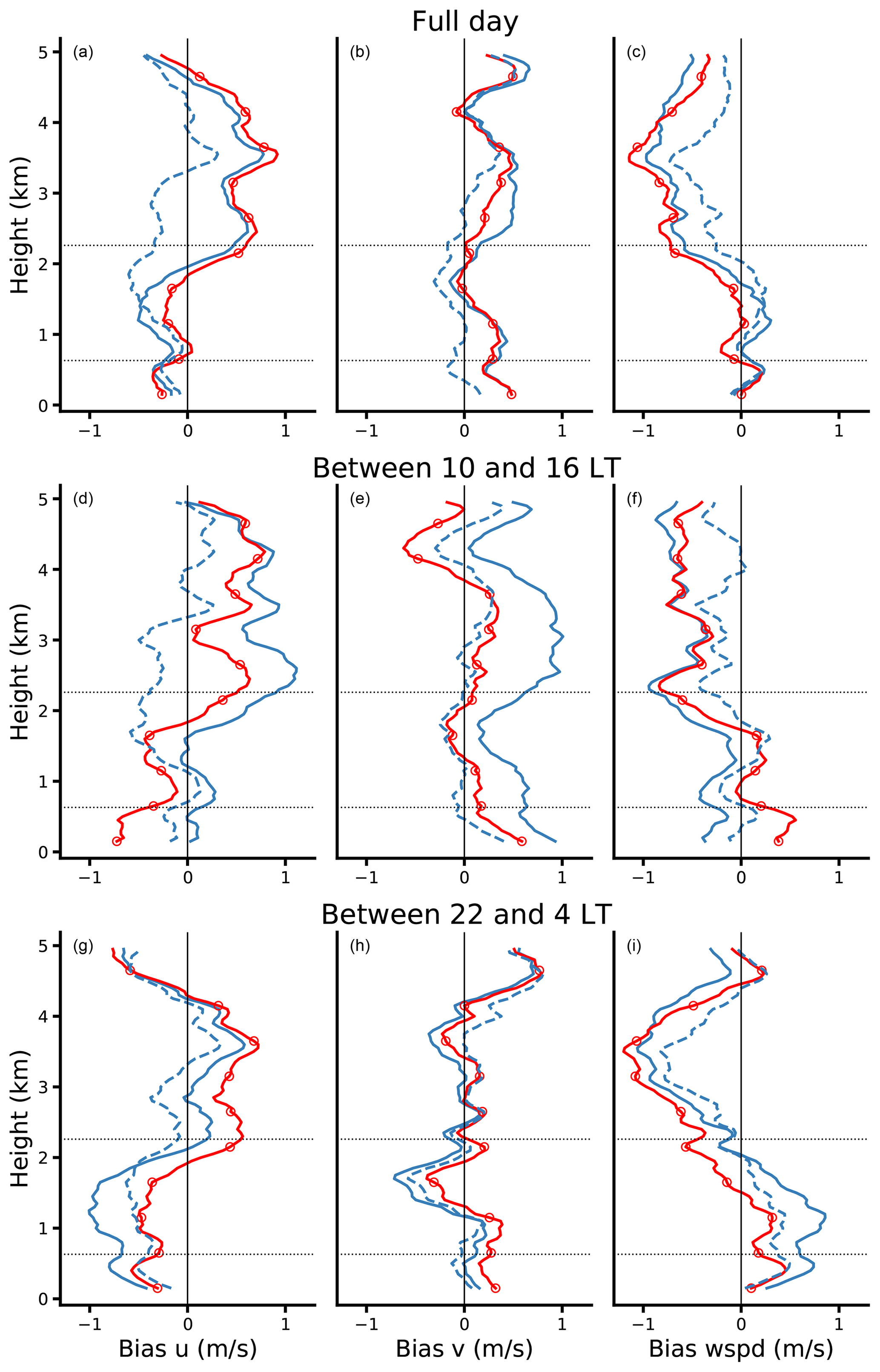
Figure 15 Mean model bias for ERA5 (dashed blue), the operational forecast (solid blue), and a forecast with the new model cycle 47r3 (red circles). The bias is shown separately for all hours of the day (a–c), for daytime between 10:00 and 16:00 LT (d–f), and for nighttime between 22:00 and 04:00 LT (g–i). The bias is calculated with respect to radiosondes. From left to right the columns refer to the bias in the zonal wind (u), meridional wind (v), and wind speed.

Although the overall mean wind profiles are similar for the two model versions (see first row in Fig. 15), there is a remarkable reduction of the daytime meridional wind bias (see Fig. 15e). With the upgraded model, the forecast becomes closer to the observations and to ERA5 at all levels. This suggests that the IFS wind bias is, at least in part, related to remote deep convection.

7 Discussion and conclusions

In this study we exploited multiple measurements from the EUREC⁴A field campaign to assess the lower-tropospheric wind bias in the operational forecasts and ERA5 reanalyses performed with the Integrated Forecasting System (IFS) of the European Centre for Medium-Range Weather Forecast (ECMWF). We focused on a 350 km × 350 km domain in the trade-winds region eastward of Barbados and investigated wind profiles extending up to 5 km height during a month-long period during boreal winter. To the authors' knowledge, this is the first time that observational vertical profiles of wind fields have been available over ocean for such an extended period of time and from various instruments.

Our analysis shows that the structure and variability of the trade winds are reasonably reproduced in the IFS, although there are biases both at the surface and throughout the troposphere, with the largest values of the bias near and above the mean trade inversion (∼ 2.3 km). In a monthly average the forecast underestimates the meridional wind component by about 0.5 m s⁻¹ in the layers below 1 km and between 2.5 and 4 km. The zonal wind component is also about 0.5 m s⁻¹ too weak between 2.5 and 4 km, while it is slightly overestimated below 1 km, in line with the known near-surface excessive easterly flow of the IFS (Belmonte Rivas and Stoffelen, 2019). The RMSE of the forecasts is larger: it increases with height from 1 m s⁻¹ near the surface to 2.5 m s⁻¹ near 3.5 km in all wind components. The RMSE is independent of the sign of the error and thus also measures positive and negative random errors that can otherwise compensate. As expected, the wind bias is smaller in ERA5, with the RMSE peaking at about 2 m s⁻¹. An analysis of the impact of the assimilation of the EUREC⁴A soundings shows that the IFS (re)analysis and forecasts are not very sensitive to the assimilation of local wind information in these undisturbed trade-winds conditions and are apparently well constrained through large-scale dynamics and other observing systems.

The wind bias in the sub-cloud layer is not constant throughout the day but exhibits a diurnal cycle just like the wind speed itself (Vial et al., 2019), which is weakest during the day at 14:00 LT (∼ 9 m s⁻¹) and strongest at midnight (∼ 10 m s⁻¹). This diurnality is overestimated by the IFS, with winds that are too weak during the day and winds that are too strong during the night, particularly in the forecasts.

The wind biases are consistent with biases in the momentum tendencies through a direct comparison of the tendencies with observed tendencies. Momentum tendencies in the model are confined to the lowest 1.5 km in the zonal direction, where the parameterized friction appears to be too large but is compensated for by larger than observed dynamical forcing, while it is missing a net acceleration of winds at levels above 2 km. In the meridional direction, the model overestimates the friction below cloud base (500 m) and misses tendency aloft, which is not well understood.

Using ICON-LEM hindcast runs over the North Atlantic corresponding to the NARVAL flight campaigns, Dixit et al. (2021) and Helfer et al. (2021) show that the cumulus friction effect is rather small at cloud base and in the cloud layer, and more friction takes place in the upper mixed layer due to sub-cloud layer overturning (coherent dry convective circulations). 10 d of EUREC⁴A large eddy simulation hindcasts are currently being investigated to shed more light on the relative contribution of dry and moist convection as well as different scales to the momentum budget.

Previous studies have suggested that missing convective variability may be the cause of the near-surface wind bias (Belmonte Rivas and Stoffelen, 2019). Removing momentum transport by shallow convection altogether reduces the wind bias near the surface, but a strong easterly wind bias near cloud base develops. The wind biases above 2 km in both the zonal and meridional wind remain. This suggests that convective momentum transport may be too active in mixing overly strong easterly momentum towards the surface and/or that there is a missing source of friction near cloud base.

A comparison with the latest IFS release (cycle 47r3), which has most significant updates in tropical deep convection, shows that the meridional wind bias (and to a lesser extent the zonal wind bias) is notably reduced during daytime. This suggests that equatorial deep convection may contribute to the bias by influencing large-scale pressure gradients. Unraveling the causes of the bias remains challenging because small-scale physics and large-scale dynamics are closely coupled. At the moment, large-domain LES hindcasts for EUREC⁴A are being analyzed to disentangle which processes and what scales critically influence the momentum budget.