the Creative Commons Attribution 4.0 License.
the Creative Commons Attribution 4.0 License.
 | 10 Oct 2022
Modelling the growth of atmospheric nitrous oxide using a global hierarchical inversion
Michael Bertolacci
Andrew Zammit-Mangion
Matthew Rigby
Paul J. Fraser
Christina M. Harth
Paul B. Krummel
Manfredi Manizza
Jens Mühle
Simon O'Doherty
Ronald G. Prinn
Ray F. Weiss
Dickon Young
Anita L. Ganesan
Nitrous oxide is a potent greenhouse gas (GHG) and ozone-depleting substance, whose atmospheric abundance has risen throughout the contemporary record. In this work, we carry out the first global hierarchical Bayesian inversion to solve for nitrous oxide emissions, which includes prior emissions with truncated Gaussian distributions and Gaussian model errors, in order to examine the drivers of the atmospheric surface growth rate. We show that both emissions and climatic variability are key drivers of variations in the surface nitrous oxide growth rate between 2011 and 2020. We derive increasing global nitrous oxide emissions, which are mainly driven by emissions between 0 and 30∘ N, with the highest emissions recorded in 2020. Our mean global total emissions for 2011–2020 of 17.2 (16.7–17.7 at the 95 % credible intervals) Tg N yr−1, comprising of 12.0 (11.2–12.8) Tg N yr−1 from land and 5.2 (4.5–5.9) Tg N yr−1 from ocean, agrees well with previous studies, but we find that emissions are poorly constrained for some regions of the world, particularly for the oceans. The prior emissions used in this and other previous work exhibit a seasonal cycle in the extra-tropical Northern Hemisphere that is out of phase with the posterior solution, and there is a substantial zonal redistribution of emissions from the prior to the posterior. Correctly characterizing the uncertainties in the system, for example in the prior emission fields, is crucial for deriving posterior fluxes that are consistent with observations. In this hierarchical inversion, the model-measurement discrepancy and the prior flux uncertainty are informed by the data, rather than solely through “expert judgement”. We show cases where this framework provides different plausible adjustments to the prior fluxes compared to inversions using widely adopted, fixed uncertainty constraints.
- Article
(5391 KB) - Full-text XML
-
Supplement
(730 KB) - BibTeX
- EndNote


Nitrous oxide (N2O) is an important greenhouse gas (GHG) that contributes substantially to the increase in radiative forcing of climate by anthropogenic activities (Myhre et al., 2013; Etminan et al., 2016). Additionally, nitrous oxide is currently the largest contributor to stratospheric ozone depletion, when considering ozone depletion potential-weighted anthropogenic emissions (Ravishankara et al., 2009). The amount of nitrous oxide in the atmosphere has risen from about 290 ppb in 1940 to 333 ppb in 2020 (Park et al., 2012; Prinn et al., 2000, 2018; Dlugokencky et al., 2021). This rise is predominantly due to increasing agricultural emissions (Davidson, 2009; Syakila and Kroeze, 2011; Tian et al., 2019). The natural sources of nitrous oxide are natural soils, biomass burning, and oceans, which are all highly uncertain in magnitude and distribution (e.g. Ciais et al., 2013). Nitrous oxide is only slowly removed from the atmosphere by photolysis and reaction with excited oxygen atoms (O(1D)) in the stratosphere, resulting in a lifetime of about 120 years (Ko et al., 2013; Prather et al., 2015).
The atmospheric abundance of nitrous oxide is monitored by several laboratories, and in this work, we use measurements taken by the National Oceanic and Atmospheric Administration (NOAA; Dlugokencky et al., 2021; Sweeney et al., 2021) and the Advanced Global Atmospheric Gases Experiment (AGAGE; Prinn et al., 2000, 2018). Figure 1 shows the atmospheric surface nitrous oxide growth rate from 2011 to 2020 based on these observations. From mid-2017 until 2019, the abundance of nitrous oxide was growing fastest in the Southern Hemisphere. Since 2000, this is only the second extended time period where the surface growth rate was led by the Southern Hemisphere. This pattern may be explained by increasing emissions within this region (Thompson et al., 2019; Tian et al., 2020; Patra et al., 2022), or by climatic variability, (e.g. the quasi-biennial oscillation (QBO)), which have been shown to be key drivers of the growth rate of surface nitrous oxide mole fraction (Ray et al., 2020; Ruiz et al., 2021).
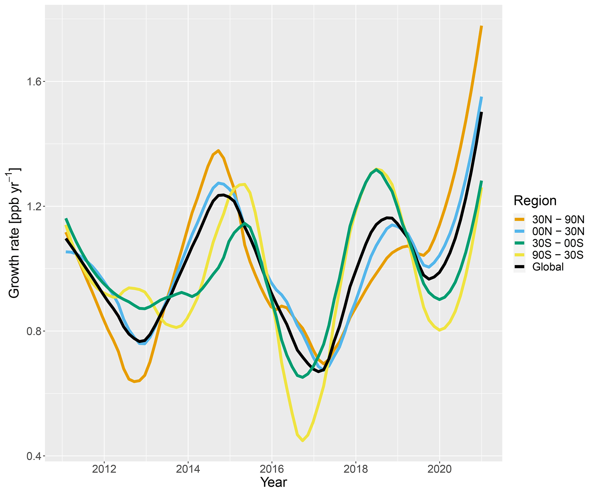
Figure 1The observed atmospheric surface nitrous oxide growth rate derived from the AGAGE and NOAA networks for each month of 2011–2020 globally (black line) and in four latitude bands (coloured lines). The observations included are detailed in Sect. 2.1, and are combined into latitude band and global totals by weighting by the cosine of the latitude. The surface growth rate is calculated as the difference in the mole fraction between the month in the displayed year and the year before, and has been smoothed using a LOESS (locally weighted smoothing) algorithm with a span of 0.3.
Previous global nitrous oxide inversions that estimated emissions from atmospheric mole fraction data include Wells et al. (2015, 2018), Thompson et al. (2019), Tian et al. (2020), and Patra et al. (2022). The latter three investigated decadal-scale emissions trends, finding that global nitrous oxide emissions have risen over the last 2 decades, with Thompson et al. (2019) attributing this rise to agricultural soils as a result of a non-linear relationship between nitrogen inputs and nitrous oxide emissions.
The agreement between previous inversion studies demonstrates that global total nitrous oxide emissions are well constrained by observations at around 17 Tg N yr−1. However, there is considerable variation on the regional scale. For example, one inversion setup in Thompson et al. (2019) derives oceanic emissions of 7.2 Tg N yr−1 over 1998–2016, whereas Patra et al. (2022) derives oceanic emissions of 2.8 Tg N yr−1 over 2000–2019. The discrepancy is also seen in developed land regions. For example, Wells et al. (2018) derives very different emissions for Europe (0.43–1.05 Tg N yr−1), depending on the inversion setup. These discrepancies suggest that new measurement or modelling approaches are required to constrain fluxes at the regional scale in global inversions.
The limited ability of atmospheric observations within global inversions to partition emissions at the regional scale means that the “bottom-up” inventory and process-modelling estimates used as prior estimates for the “top-down” inversion methods could strongly influence the inversion results. The majority of nitrous oxide emissions come from poorly understood microbial processes in the soil (Butterbach-Bahl et al., 2013), which are controlled by temperature, moisture, nitrogen inputs, and other environmental factors. Most of the remaining emissions are oceanic, and are also derived from microbial processes. Marine nitrous oxide emissions additionally require knowledge of air–sea exchange (Nevison et al., 1995; Manizza et al., 2012; Yang et al., 2020). The complex and poorly understood nature of nitrous oxide emissions means that uncertainties in the prior estimates are difficult to characterize. For example, the posterior solutions of several previous inversions have substantially altered seasonal cycles compared to bottom-up studies (e.g. Thompson et al., 2014a; Nevison et al., 2018; Wells et al., 2018). This discrepancy is thought to be due to missing freeze–thaw processes or fertilizer-application timings in process models (Wagner-Riddle et al., 2017; Nevison et al., 2018; Wells et al., 2018), or inaccuracies in top-down estimates due to model transport (Nevison et al., 2007; Thompson et al., 2014a).
Here, for the first time, we use a hierarchical Bayesian global inversion framework to estimate nitrous oxide emissions from 2011 to 2020. Previous studies investigating nitrous oxide have used either an analytical Bayesian inversion framework (e.g. Thompson et al., 2019; Tian et al., 2020; Patra et al., 2022) or a four-dimensional variational (4D-Var) method (e.g. Wells et al., 2015, 2018; Thompson et al., 2019; Tian et al., 2020). Our hierarchical Bayesian inversion framework is advantageous as both analytical and 4D-Var atmospheric inversions require specification of uncertainties on the prior fluxes and model error, both often assumed to be Gaussian, which are determined by “expert judgement”. Incorrectly specified uncertainties can significantly impact the posterior solution (Ganesan et al., 2014). The hierarchical inversion addresses this by using hyper-parameters to explore a range of possible prior uncertainties. Additionally, using Markov chain Monte Carlo (MCMC) allows the use of non-Gaussian flux distributions, which cannot easily be implemented in analytical inversion systems. These distributions are useful for gases such as nitrous oxide, as we expect land emissions to be predominantly positive. In this work, we investigate nitrous oxide emissions on a global and zonal scale using the hierarchical inversion. To help examine departures from previous inversions and explore the benefits of the hierarchical framework, we compare it to results from an analytical inversion.
2.1 Atmospheric observations
The atmospheric observations used in this work are surface measurements from 45 stations which are listed in Table 1 and mapped in Fig. 2. These observations were made by the Advanced Global Atmospheric Gases Experiment (AGAGE; Prinn et al., 2000, 2018) and as part of two National Oceanic and Atmospheric Administration (NOAA) programmes: the Halocarbons and other Atmospheric Trace Species (HATS) and the Carbon Cycle Greenhouse Gases (CCGG; Dlugokencky et al., 2021). The NOAA stations were selected based on two criteria: (i) they have nitrous oxide records for at least 6 of the years in the target time period (2010–2020) to prevent temporal inconsistencies in the inferred fluxes as stations come in and out of service, (ii) they are not heavily influenced by local nitrous oxide sources, which are determined by visual comparison of the GEOS-Chem base run (Sect. 2.2) and the observations. This filtering is necessary because the model resolution is too coarse to simulate local effects. Whilst this filtering was somewhat subjective, our results were not substantially changed if we included additional sites that appeared to experience moderate regional influence. High-frequency AGAGE data are similarly filtered to only include samples representative of background air. The background air samples are identified using the Lagrangian model, NAME (Numerical Atmospheric dispersion Modelling Environment; Jones et al., 2007), as samples where the proportion of air from the surrounding grid cells, populated areas, and the upper troposphere is low (Arnold et al., 2018).
The NOAA and AGAGE networks are on different calibration scales. To prevent this from affecting the inversion, we harmonize the networks by rescaling the AGAGE data using the method of Wells et al. (2018). This is done by using measurements from locations where both AGAGE and NOAA data are available (Cape Grim, Mace Head, Ragged Point, Tutuila, and Trinidad Head). The AGAGE and NOAA measurements made within 15 min of each other are matched, and the average ratio between the matched AGAGE and NOAA measurements (AGAGE measurements NOAA measurements) was found to be 1.0015. This ratio is used to rescale the AGAGE data. A single ratio was used for the whole time period as there was no evidence of a trend in this value over time.
Following the calibration adjustment, we compute monthly averages of the raw measurements for each station, along with the standard deviation of the measurements in that month. The monthly averages are used as observations for the inversion, and the standard deviations are used as the measurement error component of the total error budget for each observation. This is a conservative estimate of the measurement error that allows for the possibility of very high correlation between measurements within each month. If there is only one sample at a station for a month, or the calculated standard deviation is smaller than the median instrumental uncertainty reported by the data provider over all stations that month, then the median reported instrumental uncertainty is used. This method results in median measurement uncertainties of 0.26 ppb. The other component of the total error budget for each observation is model error, which we discuss in Sect. 2.3.3.
Table 1Surface stations included in the inversion. Locations of the stations are shown in Fig. 2.
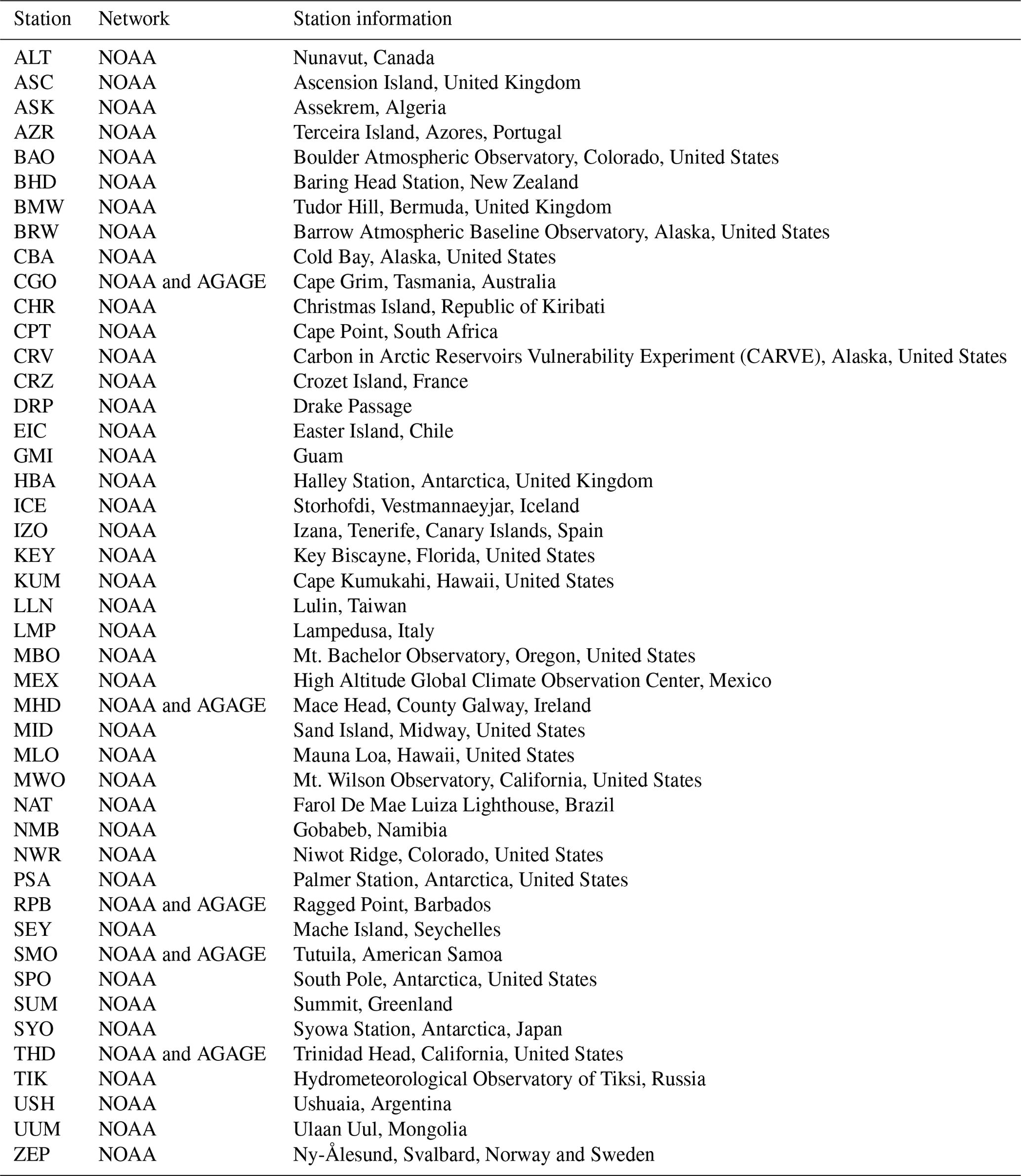

Figure 2The locations of the observations used in this work.
2.2 Nitrous oxide prior emissions and model simulations
We run model simulations to link the observations of nitrous oxide mole fractions to emissions. The simulations use the GEOS-Chem chemical transport model (http://acmg.seas.harvard.edu/geos/, last access: 28 May 2021), version 13.0.0, run with a horizontal resolution of 4∘ × 5∘ and 72 vertical levels from the surface to 0.01 hPa. The time steps are 10 min for transport and 20 min for chemistry and emissions, and use MERRA-2 meteorology (Gelaro et al., 2017).
The prior emissions we use are a combination of anthropogenic emissions from EDGARv5.0 (Crippa et al., 2019), natural soil emissions from Saikawa et al. (2013), oceanic emissions using output from the ocean model ECCO2‐Darwin (Ganesan et al., 2020), and biomass burning emissions from GFED4 (Randerson et al., 2017). The sources and their temporal resolutions are given in Table 2. The emissions from soil, oceans, and biomass burning are turned into monthly climatologies by taking the average in each calendar month in the dataset. The stratospheric loss of nitrous oxide by photolysis and reaction with O(1D) is taken from archived monthly loss frequencies from the Global Modeling Initiative (GMI; Rotman et al., 2001).
To derive an initial condition for the nitrous oxide mole fraction, we run a spin-up simulation for 10 years using repeating 2009 emissions and meteorology, starting from an atmosphere with a constant nitrous oxide mole fraction. The resulting initial condition field matches surface nitrous oxide observations to within a few ppb, has a zonal and annual mean latitude–altitude cross section of nitrous oxide mixing ratio that matches other models (Thompson et al., 2014b), and also gives a nitrous oxide lifetime of 120 years, in good agreement with Ko et al. (2013) and Prather et al. (2015). A “base” simulation is then run for 2010–2020 with time-varying meteorology and prior emissions. Further simulations using fluxes that are perturbed from the prior are used to construct basis functions, which are described in Sect. 2.3.1. In order to compare the model simulations to the observations, the modelled mole fraction is sampled at the latitude, longitude, altitude, and time of the measurements described in Sect. 2.1. Monthly mean values are created from these samples using the same method as for the observations, as in Sect. 2.1.
Crippa et al. (2019)Saikawa et al. (2013)Ganesan et al. (2020)Randerson et al. (2017)Table 2Emissions inventories used for prior emissions in this work.

2.3 WOMBAT inversion framework
The inversion uses a hierarchical Bayesian inversion framework called WOMBAT (the WOllongong Methodology for Bayesian Assimilation of Trace-gases), which has previously been used for estimating carbon dioxide emissions from satellite data (Zammit-Mangion et al., 2022). The WOMBAT framework was developed to reduce the problem of model misspecification caused by issues such as an inaccurate prior flux field and uncertainty; retrieval biases for satellite data; and possible spatio-temporal correlations in the measurement error (Zammit-Mangion et al., 2022). WOMBAT tackles these problems in the following ways: (i) specifying prior distributions on the uncertainty in the prior fluxes; (ii) modelling biases in the mole fraction data; (iii) adding a spatio-temporally correlated component of variability to the measurement error; and (iv) propagating uncertainty on all unknowns within a fully Bayesian statistical framework where inference is made using MCMC. This framework therefore provides a more statistically rigorous approach than many previous atmospheric flux inversions. A complete description of the framework for carbon dioxide inversions is given by Zammit-Mangion et al. (2022). Here, we provide a brief description of the modified framework used in this work.
This work is set up as for carbon dioxide in Zammit-Mangion et al. (2022), with four exceptions:
-
No bias in observations and no correlation in model-measurement discrepancy are considered, as the monthly data used are less likely to have correlated errors than the higher-frequency data used in Zammit-Mangion et al. (2022).
-
The fluxes are described by a Gaussian prior distribution truncated at zero to prevent negative emissions from land.
-
Fluxes are estimated using a 3-year moving window to reduce the computational cost of the inversion.
-
The autocorrelation between flux scaling factors is assumed to be zero due to the timing of the prior seasonal cycle, discussed in Sect. 3.3.2.
2.3.1 The flux process model
The true flux of nitrous oxide (Y1) is modelled as the prior flux () plus a sum of r flux basis functions (ϕj), which are weighted by scaling factors (αj). In this study, there are 3036 flux basis functions spanning the 23 TransCom regions (Fig. S1; see Gurney et al., 2002) and the 132 months of the study period. The scaling factors (α) are estimated in the inversion, and can take values of (Sect. 2.3.4). The flux process model may be written as follows:
where s is the spatial location, t denotes time, and v1 is an error term. The basis functions are set equal to the prior emissions in their corresponding region and month, and zero elsewhere. Consequently, excluding the error term, the true flux in a region is modelled as a scaling of the prior flux in that region. The error term v1 accommodates deviations between the true flux spatio-temporal patterns and those in the prior emissions.
2.3.2 The mole fraction process model
Like the flux field, the mole fraction field has a basis function representation, where each flux basis function has a corresponding response function representing the impact of the prior emissions in a TransCom region and a month on the atmospheric mole fraction field. The true mole fraction (Y2) at space–height–time location () is modelled as the prior expectation of the mole fraction field derived from the chemical transport model () plus a sum of the r response functions (ψj) which are weighted by the same scaling factors (αj) that appear in Eq. (1). The resulting mole fraction process model is as follows:
where v2 amalgamates spatio-temporal errors from the use of low-dimensional basis functions and a chemical transport model that does not simulate transport and chemistry perfectly. To construct each response function, we run a perturbed model simulation where the prior fluxes are doubled in that region and month, then subtract the simulated base mole fraction field from the field simulated under the perturbation. The perturbed simulations are run for 2 years, past which the response function is assumed to be constant in each grid cell. Running the perturbed simulations is computationally expensive, but can be reduced by running simulations in parallel and using tagged tracers within GEOS-Chem for the emissions from the different TransCom regions. These model runs are required for both an analytical inversion as well as the hierarchical inversion.
2.3.3 The mole fraction data model
The data used to constrain the nitrous oxide fluxes are the monthly mean mole fractions described in Sect. 2.1. The ith measured value (Z2,i) at space–height–time location () differs from the actual true mole fraction of the atmosphere (Y2) by the measurement error (ϵi):
Substituting Eq. (2) into Eq. (3) yields the relationship between the scaling factors (αj) and the measurements. The measurements are grouped by observation station into groups , and collected into vectors Z2,g. There are 45 observation stations in this work, and so ng is 45 in this case. The model for the gth group can be written in matrix-vector form as follows:
where the error term v2 and the measurement error ϵi have been amalgamated into an overall model-measurement discrepancy term, ξg.
We assume that the elements of ξg are distributed as independent Gaussians with mean zero and variance as follows: let ξi be the model-measurement discrepancy term for observation i in group g. We set the variance of ξi, the square root of which we call the error budget for the observation, to
where γg>0, σi is the measurement error (Sect. 2.1), and τi is the model error. The term γg is a station-specific (or equivalently, group g specific) error budget scaling factor which is estimated in the inversion. We assign the model error τi as follows. First, we calculate the standard deviation in the mole fraction of a simulation run with the prior nitrous oxide emissions in the nine horizontal model grid cells surrounding each observation. We then set τi to be the median standard deviation of the nine grid cells for each month at each station. The median (over all sites and all months) measurement uncertainty, model uncertainty, and overall error budget are 0.26, 0.08, and 0.27 ppb, respectively. This overall error budget is at the lower end of the values seen in other recent nitrous oxide inversions (Thompson et al., 2019; Tian et al., 2020; Patra et al., 2022).
The estimated model errors are likely too small, as their construction considers only spatial variability (Chen and Prinn, 2006), and ignores other errors, such as those in atmospheric transport. One benefit of our approach, is that the scaling factor γg adjusts the error budgets for the station until they better match the scale of the errors seen in the inversion. We reflect this in the prior distribution for γg, which is described in the next section.
2.3.4 The parameter model
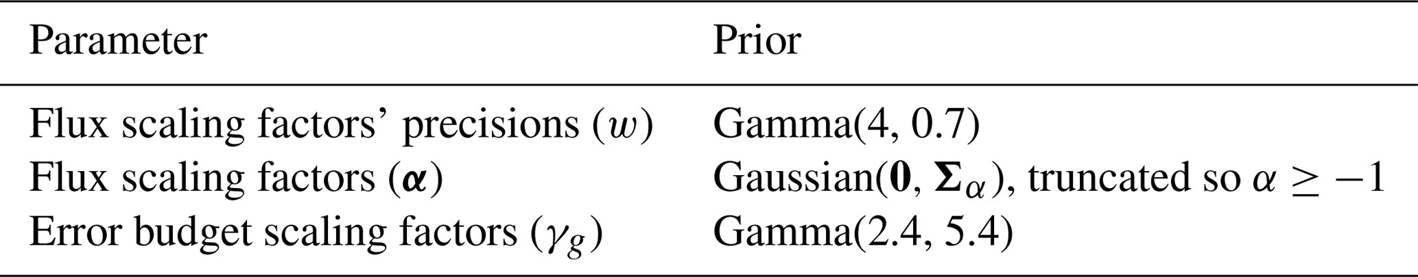
In Zammit-Mangion et al. (2022), the scaling factors (α) are assigned a multivariate Gaussian prior. In this work, to constrain the emissions to be non-negative, we instead use as prior the truncated Gaussian distribution, where denotes a multivariate Gaussian distribution with mean μ and covariance Σ, and values of α are constrained to the region F. The precision matrix is diagonal with the diagonal equal to w, and the truncation region Fα is set such that . This constrains the posterior emissions to have a sign equal to that of the prior emissions at every point in space and time. The elements of w are assigned independent gamma distributions with a shape parameter of 4 and rate parameter of 0.7 (i.e. Ga(4,0.7)). The prior mean of an element of w is thus 5.7, corresponding to a standard deviation of 0.4 (i.e. a 1σ uncertainty of 40 %) on the scaling factors.
The error budget scaling factors (γg) are given independent prior distributions of Ga(2.4,5.4). This distribution has 5 % and 95 % percentiles of 0.1 and 1.0, respectively. This corresponds to the square of the error budget being between 1 and 10 times its nominal value of , which reflects the belief that the model error is likely to be underestimated.
The relationship between the variables is summarized in Fig. 3 and the unknown parameters and their prior distributions are summarized in Table 3.

Figure 3Graphical model summarizing the relationship between the unknown parameters that are optimized in the inversion (dark grey, bottom row), intermediate variables (white, middle row), and the atmospheric mole fraction grouped by station (light grey, top row). The arrows represent the statistical dependence between the variables.
Table 3Parameters optimized in the inversion, along with their prior distributions. The values used in the measurement-error variance inflation factors' prior are given to 1 decimal place.
2.3.5 Estimation of unknown parameters
The joint posterior distribution over the unknown parameters α, w, and γ is sampled using the Gibbs sampler described by Zammit-Mangion et al. (2022), with the step to sample α modified to use the method of Pakman and Paninski (2014) to accommodate the truncated Gaussian prior. MCMC, of which a Gibbs sampler is one form, generates samples from a target distribution by simulating a Markov chain that has the target distribution as its equilibrium distribution. MCMC is beneficial as it can be used to characterize distributions that are non-Gaussian.
The method of Zammit-Mangion et al. (2022) is too computationally expensive to run over the long time period in this study. We instead use a moving window approach, which reduces the computation time from weeks to days, but is still much longer than the seconds it would take to solve analytically. Our method involves estimating the unknown parameters over a 3-year window (e.g. 2010–2012) and keeping only the parameter values inferred for the middle year (2011). This allows the first year to account for spin-up effects and the last year to contribute observations to the middle year. The next moving window (2011–2013) is then run with the prior mole fraction field for the start of the first year set to the posterior estimate from the previous window. For the last year, 2020, we use the estimates from a shorter 2019–2020 window, so fluxes from this year are more uncertain.
The results from the moving window approach were compared with varying length windows. Since the sensitivity of observations to a perturbation in the fluxes is nearly constant a year after the perturbation ceases, there was little difference between the flux scaling factors inferred by the 3-year moving window inversion and longer-length windows. Therefore, we decided to use a 3-year window to minimize computational expense while maintaining accuracy.
2.4 Analytical inversion framework
To assess the departures from previous work caused by using a hierarchical inversion, an analytical inversion is also run for comparison. The observations, error budgets, prior fluxes, and prior flux uncertainty are set up as for the WOMBAT inversion framework (Sect. 2.3), with the exception that the prior flux distribution is Gaussian rather than a truncated Gaussian. There is no adjustment of the prior flux uncertainty or the error budgets in the inversion, and since the analytical inversion is far less computationally expensive, the inversion can be run for the whole time period without the moving window approach (Sect. 2.3.5).
In the analytical inversion, the optimal flux scaling factors are found using the linear least squares approach described by Tarantola (2005), which is briefly outlined here. The centre of the posterior Gaussian (α) is given by
where Σα is the covariance matrix of α, H is the transport matrix (which transforms fluxes into modelled mole fractions), Σξ is the covariance matrix for the observations, Z2 is the observations, and is the modelled mole fraction using the prior emissions. The hyper-parameters w and γ are not solved for in this inversion, they are instead fixed values of 5.7 and 1, respectively. This results in Σα being diagonal with the diagonal values equal to 0.42, and Σξ being diagonal with diagonal values equal to the square of the error budget . The covariance matrix of the posterior Gaussian is given by
3.1 Validation of the inversion results
The inversion results can be validated by examining how well the posterior flux reproduces the observed mole fractions used in the inversion, which is presented in the Supplement. The median difference between the observed mole fraction and the prior GEOS-Chem simulation is 1.494 ppb, which is reduced to 0.012 and 0.021 ppb for the hierarchical and analytical posteriors, respectively. In order to further validate the inversion results, a GEOS-Chem simulation with the posterior fluxes from the hierarchical inversion was run. The output from this run was compared to the HIAPER Pole-to-Pole Observations (HIPPO) aircraft data, which was not used to optimize the fluxes in the inversion. This comparison is further discussed in the Supplement, but the median difference between the GEOS-Chem simulation and the observations improves from 1.36 ppb for the prior to 0.17 ppb for the hierarchical posterior.
3.2 Drivers of the surface nitrous oxide growth rate
To investigate the drivers of the observed surface nitrous oxide growth rate (Fig. 4a), we examine the prior (Fig. 4b) and posterior (Fig. 4c) estimates. The only difference between Fig. 4b and c is emissions, demonstrating that emissions are impacting the surface growth rate. To investigate the role of the climatic variability on growth rate during the last 5 years, we ran a forward GEOS-Chem simulation using the prior emissions with repeating 2015 meteorology (Fig. 4d), thus removing any interannual meteorological variations. The prior emissions in the prior are constant from 2015 onwards (Table 2), so the only difference between Fig. 4b and d is the meteorology after 2015. Most of the surface growth rate fluctuations after 2016 disappear and the surface growth rate is no longer led by the Southern Hemisphere around 2018, demonstrating that climatic variability is a key driver of the surface growth rate. Previous studies have suggested that the quasi-biennial oscillation (QBO) is an important driver of the nitrous oxide growth rate, as it modulates the stratosphere to troposphere mass flux (Ray et al., 2020; Ruiz et al., 2021).
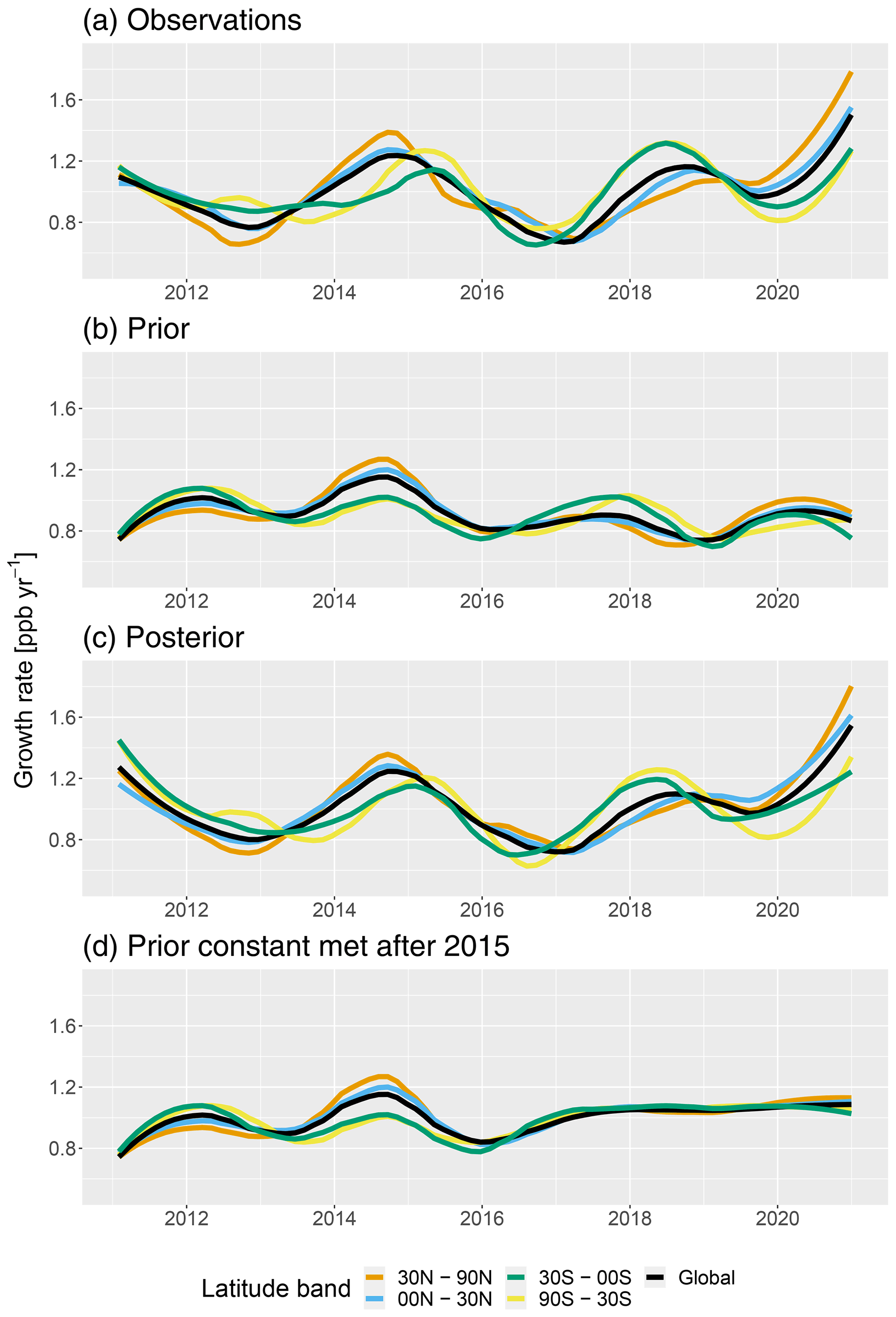
Figure 4Atmospheric nitrous oxide surface growth rate for 2011–2020 in four latitude bands and globally, for (a) the observations, (b) GEOS-Chem with the prior emissions, (c) GEOS-Chem with the posterior emissions, and (d) GEOS-Chem with repeating 2015 meteorology and prior emissions (which is the same as (b) except with constant meteorology after 2015). The growth rates have been smoothed using a LOESS (locally weighted smoothing) algorithm with a span of 0.3.
3.3 Nitrous oxide emissions
3.3.1 The global scale
Our posterior mean (and 95 % credible interval) of the global mean flux of nitrous oxide for 2011–2020 is 17.2 (16.7–17.7) Tg N yr−1, with 12.0 (11.2–12.8) Tg N yr−1 from the land (TransCom regions 0–11 in Fig. S1) and 5.2 (4.5–5.9) Tg N yr−1 from the oceans (TransCom regions 12–22 in Fig. S1). These values are within the range of other top-down estimates during this period (Wells et al., 2018; Thompson et al., 2019; Tian et al., 2020; Patra et al., 2022), as shown in Fig. 5a and b. Additionally, the inferred global total emissions show a statistically significant increasing trend over 2011–2020 (p value <0.05 when fitting a classical linear model to the posterior means), as shown in Fig. 5c. This is consistent with previous inversions which have also inferred increasing global emissions (Thompson et al., 2019; Tian et al., 2020; Patra et al., 2022), although this is the first paper to report emissions for 2020 which are likely to be the highest in 2011–2020, the cause of which is further discussed below. This emissions increase is driven by both land and ocean sectors, but we further describe below how partitioning to ocean and land could be influenced by choice of prior.
Imposed on the increasing emissions trend is substantial interannual variation, as shown in Fig. 5. Previous studies have found correlation between nitrous oxide fluxes and the El Niño–Southern Oscillation (ENSO) (Ishijima et al., 2009; Thompson et al., 2013; Ji et al., 2019; Patra et al., 2022), with the La Niña phase corresponding to higher nitrous oxide emissions. This higher emission has been attributed to increased oceanic upwelling bringing up nutrients, which increases primary production, removing oxygen from the subsurface region, which increases denitrification and nitrous oxide production (Stramma et al., 2016; Espinoza‐Morriberón et al., 2017; Ji et al., 2019). Soil emissions are also thought to vary with ENSO as a result of changing soil water content and temperature (Ishijima et al., 2009; Saikawa et al., 2013). The ENSO relationship is also seen in our work, where El Niño events in 2014–2016 and 2018–2019 correspond to lower nitrous oxide emissions, although some of the peaks and troughs in our emissions do occur in different years than in previous studies. For example, previous inversions (Thompson et al., 2019; Patra et al., 2022) infer a peak in emissions during 2013, whereas this work infers a peak in emissions during 2014. These differences are unlikely to be caused by the inversion method itself, since performing an analytical inversion rather than using a hierarchical scheme in this work produces the same pattern of interannual variability (Fig. 5). The inversions have slightly different prior emissions, but Patra et al. (2022) experimented with using different priors and the interannual variability remained unchanged. It seems that the most likely explanations for the disagreement are differences in atmospheric transport between the models and optimizing emissions for different regions. This type of systematic uncertainty is not estimated in any of the inversions presented here.
Whilst it is difficult to deduce the cause of the emissions increase in 2020 from this study, several factors could play a role. It is likely that natural cycles (e.g. the El Niño–Southern Oscillation (ENSO) (Ishijima et al., 2009; Thompson et al., 2013; Ji et al., 2019; Patra et al., 2022)) contribute to the emissions increase in 2020, alongside the longer-term trend in increasing emissions, which has been attributed to a non-linear response of nitrous oxide emissions when nitrogen input is high (Thompson et al., 2019) or an increasing emissions factor due to warming and the redistribution of emissions (Harris et al., 2022).
The impact of the hierarchical inversion can be seen by comparing it to an analytical inversion within this work, as shown in Fig. 5. On the global scale, there is very good agreement in total emissions between the two inversions performed in this work. The only year where the analytical result falls outside of the 95 % credible interval of the hierarchical result is 2020. This is because on a global scale, nitrous oxide emissions are well constrained by the observations so the inversions give consistent solutions. However, there are fewer observations to constrain the emissions in 2020 (as 2021 observations were not available). The hierarchical inversion moves further from the prior because the uncertainties in the inversion can be adjusted if the data suggest it (Sect. 3.4). The two inversions do not agree on the land and ocean emissions for 2011–2020 as well as for the global total emissions over the same time period. The land and ocean emissions are less constrained by the observations than the global total emissions, and so differences in the uncertainties in the inversions (Sect. 3.4) lead to different results. This is also the case for the zonal emissions which are discussed in Sect. 3.3.2.
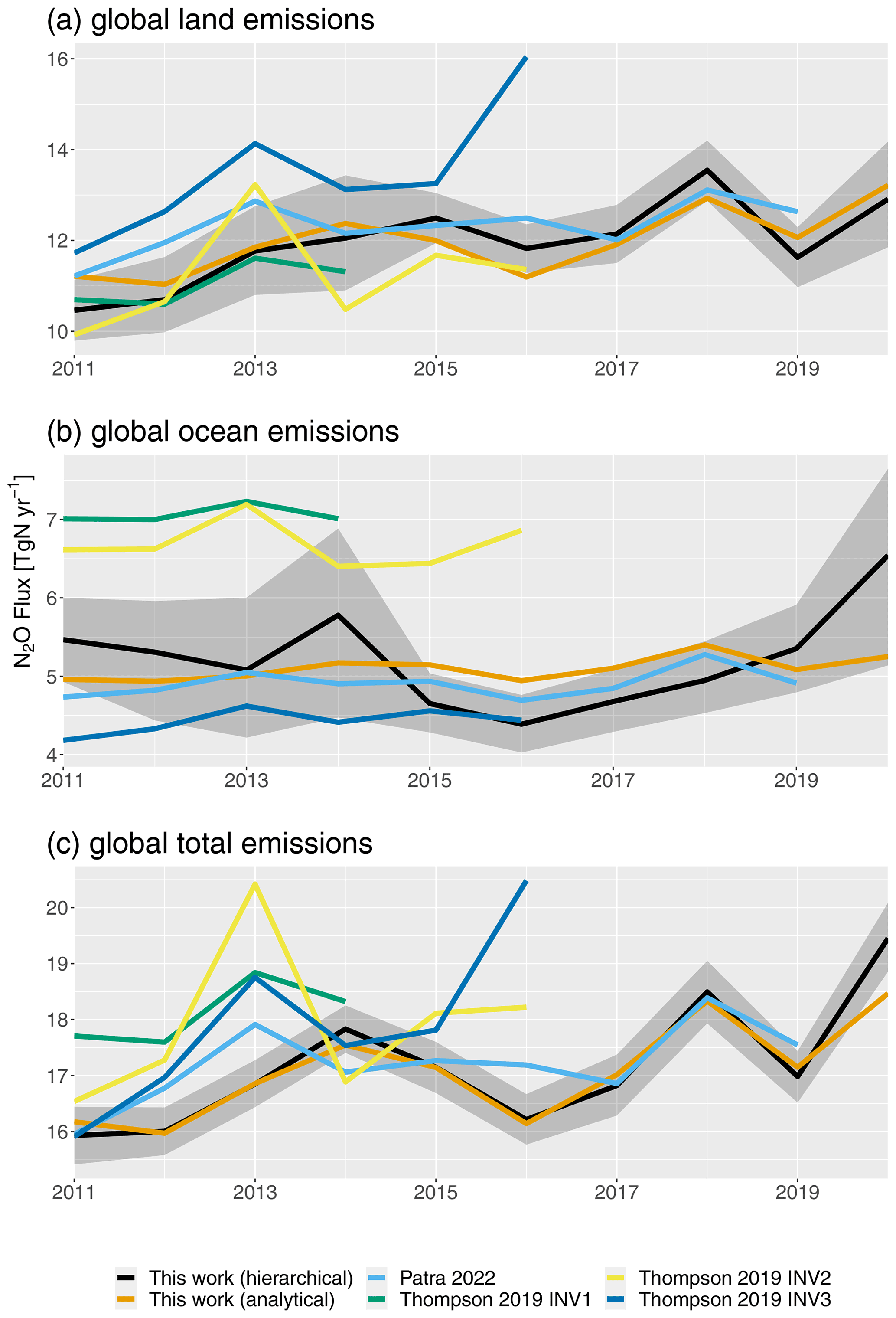
Figure 5Variation in global annual nitrous oxide emissions over 2011–2020 inferred here and in recent atmospheric inversions (Thompson et al., 2019; Patra et al., 2022), for (a) the global land, (b) the global ocean, and (c) the global total emissions. The shading represents the 95 % credible interval on the mean estimate in this work.
When total emissions are separated into land and ocean contributions, a wide range of emissions are derived by inversions depending on the prior assumptions as shown in Fig. 5a and b. We investigated the sensitivity of the inversion results in the first window (2010–2012) to having the land and ocean priors rescaled to half and double their original values with the results shown in Fig. 6. Rescaling the prior for either land or ocean results in a redistribution of the nitrous oxide emissions between land and ocean, however the global total is conserved. The redistribution is more marked when rescaling the ocean emissions. This shows that, even in a hierarchical inversion, whilst the global total emissions of nitrous oxide are well constrained by the observations, emissions on a smaller scale are strongly influenced by the prior values, in particular for the ocean regions. However, this range in prior values is not dissimilar to the range used in inversions, for example Patra et al. (2022) uses prior ocean emissions of 3.4 Tg N yr−1 whereas one inversion in Thompson et al. (2019) uses a value of over 7 Tg N yr−1. As a result, different inversion set ups will likely disagree on a regional scale until more observations are available to constrain the fluxes.

Figure 6The effect of rescaling the prior emissions over (a) land and (b) ocean on the inferred nitrous oxide flux in the first window of the inversion, inferring fluxes for the year 2011. Orange bars are the inferred fluxes when the prior was halved, blue bars are with the original prior, and green bars when the prior was doubled. The error bars represent the 95 % credible intervals on the estimates.
3.3.2 The zonal scale
We focus on zonal inferred emissions, because we believe the problems discussed in Sect. 3.3.1 imply that flux inference on a finer spatial scale is highly challenging with the background network used here, combined with our low-resolution global model setup. Therefore, we do not analyse individual TransCom regions but these are provided in the Supplement with the note that they may be unreliable estimates. The fluxes inferred on a zonal scale are shown in Fig. 7, on both annual and monthly timescales. Moving from the prior to the posterior, there has been a redistribution of emissions, with increased fluxes in the Northern Hemisphere between 0 and 30∘ N and reduced fluxes beyond 30∘ N and 30∘ S. Most of the increasing trend in global nitrous oxide emissions comes from the Northern Hemisphere between 0 and 30∘ N, although all zonal bands contribute to the interannual variability.

Figure 7Inferred nitrous oxide emissions for 2011–2020 in four zonal bands: (a) Northern Hemisphere (30–90∘ N), (b) Northern Hemisphere (0–30∘ N), (c) Southern Hemisphere (30∘ S–0∘), and (d) Southern Hemisphere (30–90∘ S). Plots on the left-hand side show annually averaged emissions and on the right-hand side show monthly emissions, where orange is the hierarchical inversion posterior, green is the analytical inversion posterior, and blue is the prior, with the shading showing the 95 % credible intervals of the hierarchical inversion posterior.
The impact of the hierarchical inversion can be seen by comparing it to an analytical inversion within this work, as shown in Fig. 7. In contrast to the well constrained global total, the inversions do infer different zonal totals, with the analytical inversion having a smaller flux and a smaller increasing trend in the Northern Hemisphere between 0 and 30∘ N. This difference between the inversions in this zonal band is mainly caused by differences in the North African and East Pacific Tropical regions (as shown in the Supplement), which can move further from the prior in the hierarchical inversion (Sect. 3.4).
Whilst it is difficult to directly compare our results to previous inversions which optimize fluxes for different regions and scales, the results are broadly similar. Previous atmospheric inversions also redistribute emissions from the extra-tropics in the prior to the tropics (Thompson et al., 2019; Patra et al., 2022), and assign an increasing trend in emissions to tropical regions, in particular South and East of Asia, Africa, tropical America, and central South America (Thompson et al., 2019; Patra et al., 2022). The main difference in this work is that no trend is derived for Asia and the Americas. This is likely a result of the hierarchical inversion which allows some regions' emissions, particularly North Africa, to be further from the prior if the data dictate it (Sect. 3.4), and hence have a larger emissions trend. In non-hierarchical inversions, it appears that the increase in emissions is spread more evenly between regions, perhaps because the prior uncertainty is more homogeneous.
Another notable difference from the prior seen in Fig. 7 is the seasonal cycle in the Northern Hemisphere between 30 and 90∘ N, which peaks as winter ends in the posterior (typically in March), rather than during summer in the prior. This seasonal cycle change has been inferred by other inversions (e.g. Thompson et al., 2014a; Nevison et al., 2018; Wells et al., 2018). According to our inversion, the land in the Northern Hemisphere causes this reversal. The prior anthropogenic emissions only vary on an annual timescale, so the land seasonal cycle predominantly comes from natural soil emissions (Saikawa et al., 2013), which does not account for processes in this latitude band such as freeze–thaw cycles or fertilizer application (Wagner-Riddle et al., 2017; Nevison et al., 2018).
3.4 The use of a hierarchical inversion
We used a hierarchical inversion scheme to characterize the uncertainties more objectively compared to previous studies. This was done by including flux scaling factor precisions and error budget scaling factors (Sect. 2.3). The mean values of these hyper-parameters over all windows inferred by the inversion, transformed into standard deviation space, are shown in Fig. 8a and b. While only a mean is presented here, the hyper-parameter values are relatively consistent between the years, although this does vary between different regions and stations (see Supplement). The shading in Fig. 8a shows the flux scaling factor standard deviation for each TransCom region. The median value for the flux scaling factor standard deviation is 0.5 (50 % prior uncertainty), but it is highly dependent on the region. Some regions have a much larger scaling factor standard deviation which means the data provide a strong enough constraint to move these regions far from the prior value. The median value is very similar to the values commonly imposed through “expert judgement” (0.5–1.0), but the hierarchical inversion scheme infers an uncertainty above 1.0 for every year in two key regions (Eurasia Temperate and North Africa). This implies that imposing a strict prior uncertainty of 100 % (or similar) in these regions may overly constrain the prior.
The second type of hyper-parameter shown in Fig. 8b are the error budget scaling factors for each measurement station. This hyper-parameter scales the error budget which includes both a measurement error and model error (Sect. 2.3). Our calculation of the error budget does not include many other types of error, such as atmospheric transport or chemistry, which the error budget scaling factors can compensate for. The median value of the error budget scaling factor (over all sites and all years) is 1.06, which corresponds to a value of 0.97 in Fig. 8b and a 3 % reduction in the error budget, but the values vary substantially by station. This means the error budget in this work is smaller than a non-hierarchical inversion would have imposed. Therefore, a non-hierarchical inversion for the same number of data points and uncertain parameters would be less data-constrained than our framework.
The variation in the error budget scaling factor between different stations is somewhat counter-intuitive, with extra-tropical stations in the Southern Hemisphere having the largest values, despite small emissions in this area. In this area, the inversion does not match the seasonal cycle or the interannual variation in the observations as well as other areas (shown in the Supplement). One of the most likely causes of the large error budget scaling factors and observational mismatch is an inadequate prior without enough flexibility to change as a result of solving on the scale of TransCom regions. The TransCom regions are particularly restrictive in the Antarctic circle (where the largest error budget scaling factors are found), as the TransCom region for Antarctica also includes Greenland and the Mediterranean Sea (see Fig. S1), limiting the potential for the fluxes in this area to adjust. Another factor could be that the extra-tropical stations in the Southern Hemisphere generally have lower error budgets before the scaling factor is applied, because of the lower spatial and temporal variability in their mole fractions. Additionally, because of the low emissions in this area, the variations in atmospheric nitrous oxide mole fractions are mainly driven by atmospheric transport, which the inversion cannot adjust.
The analytical inversion does not include these hyper-parameters and hence, the uncertainties in the inversion are not as reliable as in the hierarchical inversion. Therefore, the analytical inversion presented in this work should not be interpreted as an alternative solution, but rather as a way to examine departures from previous work.
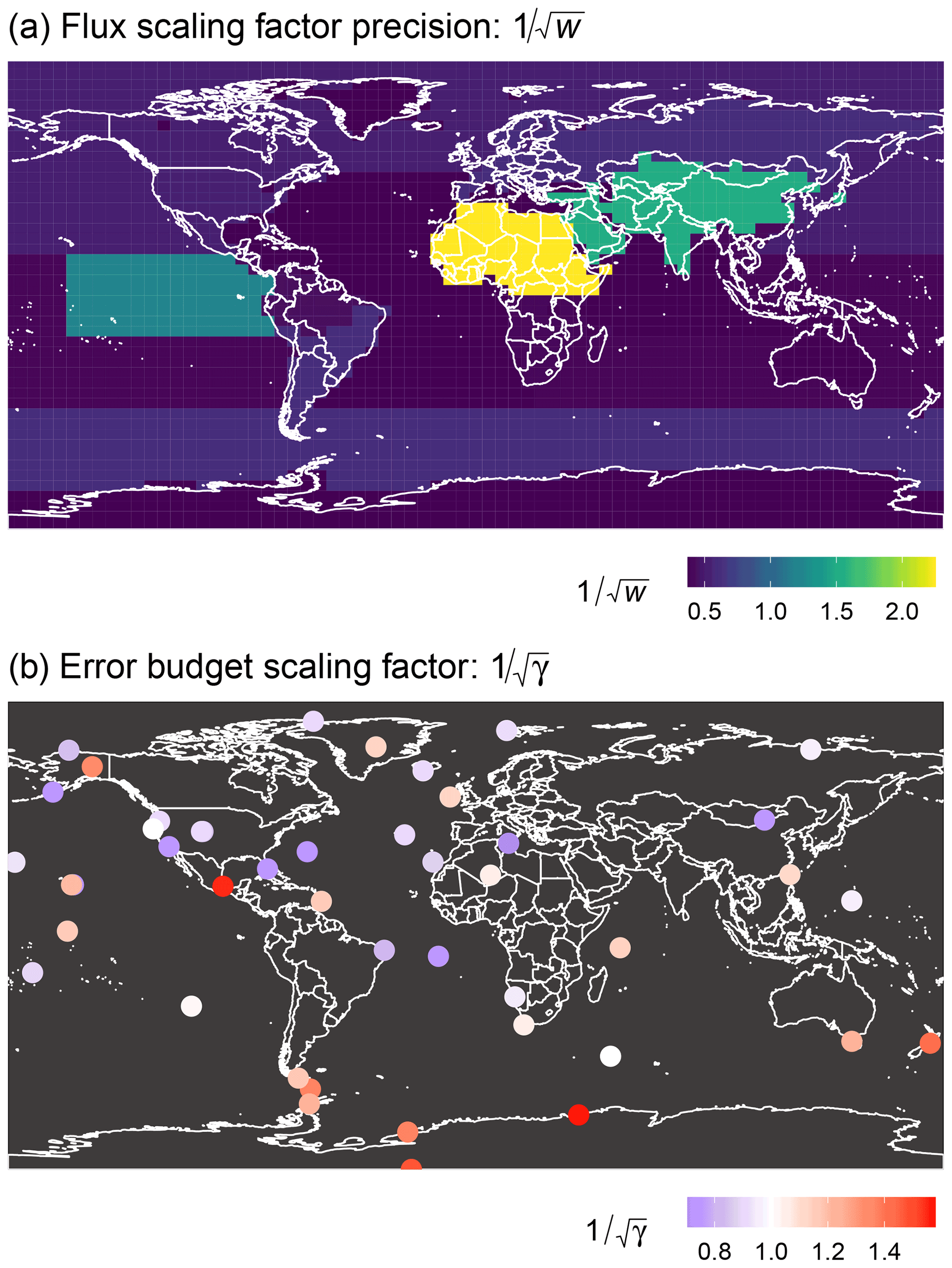
Figure 8The inferred hyper-parameters transformed into a standard deviation scale. The shading in (a) represents the mean uncertainty in the prior emissions () which is solved for each TransCom region on an annual basis. The coloured dots in (b) represent the mean error budget scaling factor () which is solved for each measurement station.
We carried out the first hierarchical inversion to solve for global nitrous oxide emissions. We find that global emissions have increased between 2011 and 2020, with substantial interannual variability. Emissions derived for 2020 were the highest in this period, 19.5 (95 % credible interval: 18.9–20.1) Tg N yr−1 due to an increase of emissions in the tropics. On annual timescales, our estimated global emissions differ from other studies, likely due to differences in atmospheric chemical transport models and optimizing emissions for different regions, rather than the inversion method. We show that the recent atmospheric surface growth rate fluctuations are likely to be driven by both emissions and interannual variability in transport.
At the zonal scale, we find several issues with the bottom-up emission estimates used as a prior. The posterior seasonal cycle in the extra-tropical Northern Hemisphere is out of phase with the prior. This may be because the agricultural soil emissions in the prior are only on an annual resolution, and/or because natural soil emissions do not include important processes such as freeze–thaw cycles. Additionally, there has been a substantial redistribution of emissions from the extra-tropics in the prior to the tropics in the Northern Hemisphere in the posterior. This is the zonal band where most of the globally increasing trend comes from over the time period studied.
By adapting and extending the hierarchical inversion framework of Zammit-Mangion et al. (2022), we have shown that inversions for nitrous oxide can be performed that do not rely on rigid assumptions regarding error budgets or the uncertainty of the fluxes. Our uncertainties are estimated by the inversion and are generally smaller than those that would be used in a non-hierarchical inversion for the same number of data points and uncertain parameters, and therefore our inversion is more data-constrained. Additionally, our uncertainties vary greatly across different stations and regions, which is not considered in previous non-hierarchical studies. Two innovations in this work over Zammit-Mangion et al. (2022) are the moving window technique, which allows for more efficient computation of fluxes over very long time periods (∼10 years or longer), and the incorporation of a truncated Gaussian prior to impose sign constraints on the emissions. The method presented here serves as a framework that can be extended to higher-resolution models (potentially allowing more reliable regional emissions inference) and larger datasets.
The code and data for this work can be found at https://doi.org/10.17605/OSF.IO/SN539 (Stell, 2022). The GEOS-Chem model is available to be downloaded at http://www.geos-chem.org (last access: 28 May 2021; The International GEOS-Chem User Community, 2021, https://doi.org/10.5281/zenodo.4618180). The atmospheric observations can be obtained from the data providers: https://www.esrl.noaa.gov/gmd/ (last access: 28 May 2021; Dlugokencky et al., 2021, https://doi.org/10.7289/V5CN725S; Sweeney et al., 2021, https://doi.org/10.7289/V5N58JMF) for NOAA and https://agage.mit.edu (last access: 28 May 2021; Prinn et al., 2021, https://doi.org/10.15485/1781803) for AGAGE.
The supplement related to this article is available online at: https://doi.org/10.5194/acp-22-12945-2022-supplement.
ACS wrote the code (excluding the WOMBAT framework), performed the calculations, and led the writing of the manuscript. MB and AZM wrote the original WOMBAT framework and MB helped to develop the framework further for this work. PJF, CMH, PBK, JM, SO, RGP, RFW, and DY provided the AGAGE atmospheric measurements. XL provided the NOAA atmospheric measurements. MM provided ocean model output and helped to interpret the results. ACS, MB, AZM, MR, and ALG designed the research. All authors contributed to the manuscript.
The contact author has declared that none of the authors has any competing interests.
Neither UKRI nor any of the partner institutions are responsible for the views advanced here.
Publisher's note: Copernicus Publications remains neutral with regard to jurisdictional claims in published maps and institutional affiliations.
This work results from research funded by UK Research and Innovation (UKRI) under the South Asian Nitrogen Hub (SANH). The project team includes partners from across South Asia and the UK. Angharad C. Stell was supported by SANH. Michael Bertolacci and Andrew Zammit-Mangion were supported by the Australian Research Council (ARC) Discovery Project (DP). The MHD, THD, RPB, SMO, and CGO AGAGE stations are supported by the National Aeronautics and Space Administration (NASA). Support also comes from the UK Department for Business, Energy & Industrial Strategy (BEIS) for MHD, NOAA for RPB, and the Commonwealth Scientific and Industrial Research Organization (CSIRO) and the Bureau of Meteorology (Australia) for CGO. This work is supported in part by the Cooperative Agreement between NOAA and the Cooperative Institute for Research in Environmental Sciences (CIRES).
This research has been supported by the UK Research and Innovation (grant no. NE/S009019/1), the Australian Research Council (grant no. DP190100180), and the National Aeronautics and Space Administration (grant nos. NX16AC98G, NNX16AC97G, and NNX16AC96G).
This paper was edited by Andreas Hofzumahaus and reviewed by two anonymous referees.
Arnold, T., Manning, A. J., Kim, J., Li, S., Webster, H., Thomson, D., Mühle, J., Weiss, R. F., Park, S., and O'Doherty, S.: Inverse modelling of CF4 and NF3 emissions in East Asia, Atmos. Chem. Phys., 18, 13305–13320, https://doi.org/10.5194/acp-18-13305-2018, 2018. a
Butterbach-Bahl, K., Baggs, E. M., Dannenmann, M., Kiese, R., and Zechmeister-Boltenstern, S.: Nitrous oxide emissions from soils: how well do we understand the processes and their controls?, Philos. T. Roy. Soc. B, 368, 20130122, https://doi.org/10.1098/rstb.2013.0122, 2013. a
Chen, Y.-H. and Prinn, R. G.: Estimation of atmospheric methane emissions between 1996 and 2001 using a three-dimensional global chemical transport model, J. Geophys. Res.-Atmos., 111, D10307, https://doi.org/10.1029/2005JD006058, 2006. a
Ciais, P., Sabine, C., Bala, G., Bopp, L., Brovkin, V., Canadell, J., Chhabra, A., DeFries, R., Galloway, J., Heimann, M., Jones, C., Le Quéré, C., Myneni, R. B., Piao, S., and Thornton, P.: Carbon and other biogeochemical cycles in climate change 2013 – The physical science basis, in: Working Group I Contribution to the Fifth Assessment Report of the Intergovernmental Panel on Climate Change, edited by: [Stocker, T. F., Qin, D., Plattner, G.-K., Tignor, M., Allen, S. K., Boschung, J., Nauels, A., Xia, Y., Bex, V. and Midgley, P. M., Cambridge University Press, Cambridge, United Kingdom and New York, NY, USA, 465–570, 2013. a
Crippa, M., Oreggioni, G., Guizzardi, D., Muntean, M., Schaaf, E., Lo Vullo, E., Solazzo, E., Monforti-Ferrario, F., Olivier, J., Vignati, E., European Commission, and Joint Research Centre: Fossil CO2 and GHG emissions of all world countries: 2019 report, Publications Office of the European Union, Luxembourg, https://doi.org/10.2760/687800, 2019. a, b
Davidson, E. A.: The contribution of manure and fertilizer nitrogen to atmospheric nitrous oxide since 1860, Nat. Geosci., 2, 659–662, https://doi.org/10.1038/ngeo608, 2009. a
Dlugokencky, E., Crotwell, A., Lang, P., Higgs, J., Vaughn, B., Englund, S., Novelli, P., Wolter, S., Mund, J., Moglia, E., Crotwell, M., and NOAA ESRL: Earth System Research Laboratory Carbon Cycle and Greenhouse Gases Group Flask-Air Sample Measurements of CO2, CH4, CO, N2O, H2, SF6 and isotopic ratios at Global and Regional Background Sites, 1967–Present, Version 2.0, NOAA National Centers for Environmental Information [data set], https://doi.org/10.7289/V5CN725S, 2021. a, b, c, d
Espinoza‐Morriberón, D., Echevin, V., Colas, F., Tam, J., Ledesma, J., Vásquez, L., and Graco, M.: Impacts of El Niño events on the Peruvian upwelling system productivity, J. Geophys. Res.-Oceans, 122, 5423–5444, https://doi.org/10.1002/2016JC012439, 2017. a
Etminan, M., Myhre, G., Highwood, E. J., and Shine, K. P.: Radiative forcing of carbon dioxide, methane, and nitrous oxide: A significant revision of the methane radiative forcing, Geophys. Res. Lett., 43, 12614–12623, https://doi.org/10.1002/2016GL071930, 2016. a
Ganesan, A. L., Rigby, M., Zammit-Mangion, A., Manning, A. J., Prinn, R. G., Fraser, P. J., Harth, C. M., Kim, K.-R., Krummel, P. B., Li, S., Mühle, J., O'Doherty, S. J., Park, S., Salameh, P. K., Steele, L. P., and Weiss, R. F.: Characterization of uncertainties in atmospheric trace gas inversions using hierarchical Bayesian methods, Atmos. Chem. Phys., 14, 3855–3864, https://doi.org/10.5194/acp-14-3855-2014, 2014. a
Ganesan, A. L., Manizza, M., Morgan, E. J., Harth, C. M., Kozlova, E., Lueker, T., Manning, A. J., Lunt, M. F., Mühle, J., Lavric, J. V., Heimann, M., Weiss, R. F., and Rigby, M.: Marine Nitrous Oxide Emissions From Three Eastern Boundary Upwelling Systems Inferred From Atmospheric Observations, Geophys. Res. Lett., 47, e2020GL087822, https://doi.org/10.1029/2020GL087822, 2020. a, b
Gelaro, R., McCarty, W., Suárez, M. J., Todling, R., Molod, A., Takacs, L., Randles, C. A., Darmenov, A., Bosilovich, M. G., Reichle, R., Wargan, K., Coy, L., Cullather, R., Draper, C., Akella, S., Buchard, V., Conaty, A., da Silva, A. M., Gu, W., Kim, G.-K., Koster, R., Lucchesi, R., Merkova, D., Nielsen, J. E., Partyka, G., Pawson, S., Putman, W., Rienecker, M., Schubert, S. D., Sienkiewicz, M., and Zhao, B.: The Modern-Era Retrospective Analysis for Research and Applications, Version 2 (MERRA-2), J. Climate, 30, 5419–5454, https://doi.org/10.1175/JCLI-D-16-0758.1, 2017. a
Gurney, K. R., Law, R. M., Denning, A. S., Rayner, P. J., Baker, D., Bousquet, P., Bruhwiler, L., Chen, Y.-H., Ciais, P., Fan, S., Fung, I. Y., Gloor, M., Heimann, M., Higuchi, K., John, J., Maki, T., Maksyutov, S., Masarie, K., Peylin, P., Prather, M., Pak, B. C., Randerson, J., Sarmiento, J., Taguchi, S., Takahashi, T., and Yuen, C.-W.: Towards robust regional estimates of CO2 sources and sinks using atmospheric transport models, Nature, 415, 626–630, https://doi.org/10.1038/415626a, 2002. a
Harris, E., Yu, L., Wang, Y.-P., Mohn, J., Henne, S., Bai, E., Barthel, M., Bauters, M., Boeckx, P., Dorich, C., Farrell, M., Krummel, P. B., Loh, Z. M., Reichstein, M., Six, J., Steinbacher, M., Wells, N. S., Bahn, M., and Rayner, P.: Warming and redistribution of nitrogen inputs drive an increase in terrestrial nitrous oxide emission factor, Nat. Commun., 13, 4310, https://doi.org/10.1038/s41467-022-32001-z, 2022. a
Ishijima, K., Nakazawa, T., and Aoki, S.: Variations of atmospheric nitrous oxide concentration in the northern and western Pacific, Tellus B, 61, 408–415, https://doi.org/10.1111/j.1600-0889.2008.00406.x, 2009. a, b, c
Ji, Q., Altabet, M. A., Bange, H. W., Graco, M. I., Ma, X., Arévalo-Martínez, D. L., and Grundle, D. S.: Investigating the effect of El Niño on nitrous oxide distribution in the eastern tropical South Pacific, Biogeosciences, 16, 2079–2093, https://doi.org/10.5194/bg-16-2079-2019, 2019. a, b, c
Jones, A., Thomson, D., Hort, M., and Devenish, B.: The U.K. Met Office's Next-Generation Atmospheric Dispersion Model, NAME III, in: Air Pollution Modeling and Its Application XVII, edited by: Borrego C. and Norman AL., 580–589, Springer, Boston, MA, https://doi.org/10.1007/978-0-387-68854-1_62, 2007. a
Ko, M. K. W., Newman, P. A., Reimann, S., and Strahan, S. E.: SPARC Report on Lifetimes of Stratospheric Ozone-Depleting Substances, Their Replacements, and Related Species, Tech. rep., SPARC Office, http://www.sparc-climate.org/publications/sparc-reports/ (last access: 7 July 2022), SPARC Publication Title: SPARC Report vol. 6, 2013. a, b
Manizza, M., Keeling, R. F., and Nevison, C. D.: On the processes controlling the seasonal cycles of the air–sea fluxes of O2 and N2O: A modelling study, Tellus B, 64, 18429, https://doi.org/10.3402/tellusb.v64i0.18429, 2012. a
Myhre, G., Shindell, D., Bréon, F.-M., Collins, W., Fuglestvedt, J., Huang, J., Koch, D., Lamarque, J.-F., Lee, D., Mendoza, B., Nakajima, T., Robock, A., Stephens, G., Takemura, T., and Zhang, H.: Anthropogenic and Natural Radiative Forcing, in: Climate Change 2013: The Physical Science Basis, Contribution of Working Group I to the Fifth Assessment Report of the Intergovernmental Panel on Climate Change edited by: Stocker, T.F., Qin, D., Plattner, G.-K., Tignor, M., Allen, S.K., Boschung, J., Nauels, A., Xia, Y., Bex, V., and Midgley, P.M., 82, Cambridge University Press, Cambridge, United Kingdom and New York, NY, USA, 2013. a
Nevison, C., Andrews, A., Thoning, K., Dlugokencky, E., Sweeney, C., Miller, S., Saikawa, E., Benmergui, J., Fischer, M., Mountain, M., and Nehrkorn, T.: Nitrous Oxide Emissions Estimated With the CarbonTracker‐Lagrange North American Regional Inversion Framework, Global Biogeochem. Cycles, 32, 463–485, https://doi.org/10.1002/2017GB005759, 2018. a, b, c, d
Nevison, C. D., Weiss, R. F., and Erickson, D. J.: Global oceanic emissions of nitrous oxide, J. Geophys. Res., 100, 15809–15820, https://doi.org/10.1029/95JC00684, 1995. a
Nevison, C. D., Mahowald, N. M., Weiss, R. F., and Prinn, R. G.: Interannual and seasonal variability in atmospheric N2O, Global Biogeochem. Cycles, 21, GB3017, https://doi.org/10.1029/2006GB002755, 2007. a
Pakman, A. and Paninski, L.: Exact Hamiltonian Monte Carlo for Truncated Multivariate Gaussians, J. Comput. Graphical Stat., 23, 518–542, https://doi.org/10.1080/10618600.2013.788448, 2014. a
Park, S., Croteau, P., Boering, K. A., Etheridge, D. M., Ferretti, D., Fraser, P. J., Kim, K.-R., Krummel, P. B., Langenfelds, R. L., van Ommen, T. D., Steele, L. P., and Trudinger, C. M.: Trends and seasonal cycles in the isotopic composition of nitrous oxide since 1940, Nat. Geosci., 5, 261–265, https://doi.org/10.1038/ngeo1421, 2012. a
Patra, P. K., Dlugokencky, E. J., Elkins, J. W., Dutton, G. S., Tohjima, Y., Sasakawa, M., Ito, A., Weiss, R. F., Manizza, M., Krummel, P. B., Prinn, R. G., O'Doherty, S., Bianchi, D., Nevison, C., Solazzo, E., Lee, H., Joo, S., Kort, E. A., Maity, S., and Takigawa, M.: Forward and Inverse Modelling of Atmospheric Nitrous Oxide Using MIROC4-Atmospheric Chemistry-Transport Model, J. Meteorol. Soc. Japan. Ser. II, 100, 361–386, https://doi.org/10.2151/jmsj.2022-018, 2022. a, b, c, d, e, f, g, h, i, j, k, l, m, n, o
Prather, M. J., Hsu, J., DeLuca, N. M., Jackman, C. H., Oman, L. D., Douglass, A. R., Fleming, E. L., Strahan, S. E., Steenrod, S. D., Søvde, O. A., Isaksen, I. S. A., Froidevaux, L., and Funke, B.: Measuring and modeling the lifetime of nitrous oxide including its variability, J. Geophys. Res.-Atmos., 120, 5693–5705, https://doi.org/10.1002/2015JD023267, 2015. a, b
Prinn, R. G., Weiss, R. F., Fraser, P. J., Simmonds, P. G., Cunnold, D. M., Alyea, F. N., O'Doherty, S., Salameh, P., Miller, B. R., Huang, J., Wang, R. H. J., Hartley, D. E., Harth, C., Steele, L. P., Sturrock, G., Midgley, P. M., and McCulloch, A.: A history of chemically and radiatively important gases in air deduced from ALE/GAGE/AGAGE, J. Geophys. Res.-Atmos., 105, 17751–17792, https://doi.org/10.1029/2000JD900141, 2000. a, b, c
Prinn, R. G., Weiss, R. F., Arduini, J., Arnold, T., DeWitt, H. L., Fraser, P. J., Ganesan, A. L., Gasore, J., Harth, C. M., Hermansen, O., Kim, J., Krummel, P. B., Li, S., Loh, Z. M., Lunder, C. R., Maione, M., Manning, A. J., Miller, B. R., Mitrevski, B., Mühle, J., O'Doherty, S., Park, S., Reimann, S., Rigby, M., Saito, T., Salameh, P. K., Schmidt, R., Simmonds, P. G., Steele, L. P., Vollmer, M. K., Wang, R. H., Yao, B., Yokouchi, Y., Young, D., and Zhou, L.: History of chemically and radiatively important atmospheric gases from the Advanced Global Atmospheric Gases Experiment (AGAGE), Earth Syst. Sci. Data, 10, 985–1018, https://doi.org/10.5194/essd-10-985-2018, 2018. a, b, c
Prinn, R., Weiss, R., Arduini, J., Arnold, T., DeWitt, H. L., Fraser, P., Ganesan, A., Gasore, J., Harth, C., Hermansen, O., Kim, J., Krummel, P., Li, S., Loh, Z., Lunder, C., Maione, M., Manning, A., Miller, B., Mitrevski, B., Mühle, J., O'Doherty, S., Park, S., Reimann, S., Rigby, M., Saito, T., Salameh, P., Schmidt, R., Simmonds, P., Steele, P., Vollmer, M., Wang, H., Yao, B., Young, D., and Zhou, L.: In-situ measurements of chemically and radiatively important atmospheric gases from the Advanced Global Atmospheric Gas Experiment (AGAGE) and affiliated stations. The Advanced Global Atmospheric Gases Experiment (AGAGE) Data, ESS-DIVE repository [data set], https://doi.org/10.15485/1781803, 2021. a
Randerson, J., van der Werf, G., Giglio, L., Collatz, G., and Kasibhatla, P.: Global Fire Emissions Database, Version 4.1 (GFEDv4), ORNL DAAC [data set], https://doi.org/10.3334/ORNLDAAC/1293, 2017. a, b
Ravishankara, A. R., Daniel, J. S., and Portmann, R. W.: Nitrous Oxide (N2O): The Dominant Ozone-Depleting Substance Emitted in the 21st Century, Science, 326, 123–125, https://doi.org/10.1126/science.1176985, 2009. a
Ray, E. A., Portmann, R. W., Yu, P., Daniel, J., Montzka, S. A., Dutton, G. S., Hall, B. D., Moore, F. L., and Rosenlof, K. H.: The influence of the stratospheric Quasi-Biennial Oscillation on trace gas levels at the Earth’s surface, Nat. Geosci., 13, 22–27, https://doi.org/10.1038/s41561-019-0507-3, 2020. a, b
Rotman, D. A., Tannahill, J. R., Kinnison, D. E., Connell, P. S., Bergmann, D., Proctor, D., Rodriguez, J. M., Lin, S. J., Rood, R. B., Prather, M. J., Rasch, P. J., Considine, D. B., Ramaroson, R., and Kawa, S. R.: Global Modeling Initiative assessment model: Model description, integration, and testing of the transport shell, J. Geophys. Res.-Atmos., 106, 1669–1691, https://doi.org/10.1029/2000JD900463, 2001. a
Ruiz, D. J., Prather, M. J., Strahan, S. E., Thompson, R. L., Froidevaux, L., and Steenrod, S. D.: How Atmospheric Chemistry and Transport Drive Surface Variability of N2O and CFC‐11, J. Geophys. Res.-Atmos., 126, e2020JD033979, https://doi.org/10.1029/2020JD033979, 2021. a, b
Saikawa, E., Schlosser, C. A., and Prinn, R. G.: Global modeling of soil nitrous oxide emissions from natural processes, Global Biogeochem. Cycles, 27, 972–989, https://doi.org/10.1002/gbc.20087, 2013. a, b, c, d
Stell, A. C.: Modelling the growth of atmospheric nitrous oxide using a hierarchical inversion, OSF [code and data], https://doi.org/10.17605/OSF.IO/SN539, 2022. a
Stramma, L., Fischer, T., Grundle, D. S., Krahmann, G., Bange, H. W., and Marandino, C. A.: Observed El Niño conditions in the eastern tropical Pacific in October 2015, Ocean Sci., 12, 861–873, https://doi.org/10.5194/os-12-861-2016, 2016. a
Sweeney, C., Higgs, J., Wolter, S., Crotwell, A., Neff, D., Dlugokencky, E., Lang, P., Novelli, P., Mund, J., Moglia, E., Crotwell, M., and NOAA ESRL: Earth System Research Laboratory Carbon Cycle and Greenhouse Gases Group Flask-Air Sample Measurements of CO2, CH4, CO, N2O, H2, and SF6 from the Aircraft Program, 1992–Present, Version 2.0, NOAA National Centers for Environmental Information [data set], https://doi.org/10.7289/V5N58JMF, 2021. a, b
Syakila, A. and Kroeze, C.: The global nitrous oxide budget revisited, Greenhouse Gas Measurement and Management, 1, 17–26, https://doi.org/10.3763/ghgmm.2010.0007, 2011. a
Tarantola, A.: Inverse Problem Theory and Methods for Model Parameter Estimation, Society for Industrial and Applied Mathematics, https://doi.org/10.1137/1.9780898717921, 2005. a
The International GEOS-Chem User Community: geoschem/GCClassic: GEOS-Chem 13.0.0 (13.0.0), Zenodo [code], https://doi.org/10.5281/zenodo.4618180, 2021. a
Thompson, R. L., Dlugokencky, E., Chevallier, F., Ciais, P., Dutton, G., Elkins, J. W., Langenfelds, R. L., Prinn, R. G., Weiss, R. F., Tohjima, Y., O'Doherty, S., Krummel, P. B., Fraser, P., and Steele, L. P.: Interannual variability in tropospheric nitrous oxide, Geophys. Res. Lett., 40, 4426–4431, https://doi.org/10.1002/grl.50721, 2013. a, b
Thompson, R. L., Ishijima, K., Saikawa, E., Corazza, M., Karstens, U., Patra, P. K., Bergamaschi, P., Chevallier, F., Dlugokencky, E., Prinn, R. G., Weiss, R. F., O'Doherty, S., Fraser, P. J., Steele, L. P., Krummel, P. B., Vermeulen, A., Tohjima, Y., Jordan, A., Haszpra, L., Steinbacher, M., Van der Laan, S., Aalto, T., Meinhardt, F., Popa, M. E., Moncrieff, J., and Bousquet, P.: TransCom N2O model inter-comparison – Part 2: Atmospheric inversion estimates of N2O emissions, Atmos. Chem. Phys., 14, 6177–6194, https://doi.org/10.5194/acp-14-6177-2014, 2014a. a, b, c
Thompson, R. L., Patra, P. K., Ishijima, K., Saikawa, E., Corazza, M., Karstens, U., Wilson, C., Bergamaschi, P., Dlugokencky, E., Sweeney, C., Prinn, R. G., Weiss, R. F., O'Doherty, S., Fraser, P. J., Steele, L. P., Krummel, P. B., Saunois, M., Chipperfield, M., and Bousquet, P.: TransCom N2O model inter-comparison – Part 1: Assessing the influence of transport and surface fluxes on tropospheric N2O variability, Atmos. Chem. Phys., 14, 4349–4368, https://doi.org/10.5194/acp-14-4349-2014, 2014b. a
Thompson, R. L., Lassaletta, L., Patra, P. K., Wilson, C., Wells, K. C., Gressent, A., Koffi, E. N., Chipperfield, M. P., Winiwarter, W., Davidson, E. A., Tian, H., and Canadell, J. G.: Acceleration of global N2O emissions seen from two decades of atmospheric inversion, Nat. Clim. Change, 9, 993–998, https://doi.org/10.1038/s41558-019-0613-7, 2019. a, b, c, d, e, f, g, h, i, j, k, l, m, n, o
Tian, H., Yang, J., Xu, R., Lu, C., Canadell, J. G., Davidson, E. A., Jackson, R. B., Arneth, A., Chang, J., Ciais, P., Gerber, S., Ito, A., Joos, F., Lienert, S., Messina, P., Olin, S., Pan, S., Peng, C., Saikawa, E., Thompson, R. L., Vuichard, N., Winiwarter, W., Zaehle, S., and Zhang, B.: Global soil nitrous oxide emissions since the preindustrial era estimated by an ensemble of terrestrial biosphere models: Magnitude, attribution, and uncertainty, Global Change Biol., 25, 640–659, https://doi.org/10.1111/gcb.14514, 2019. a
Tian, H., Xu, R., Canadell, J. G., Thompson, R. L., Winiwarter, W., Suntharalingam, P., Davidson, E. A., Ciais, P., Jackson, R. B., Janssens-Maenhout, G., Prather, M. J., Regnier, P., Pan, N., Pan, S., Peters, G. P., Shi, H., Tubiello, F. N., Zaehle, S., Zhou, F., Arneth, A., Battaglia, G., Berthet, S., Bopp, L., Bouwman, A. F., Buitenhuis, E. T., Chang, J., Chipperfield, M. P., Dangal, S. R. S., Dlugokencky, E., Elkins, J. W., Eyre, B. D., Fu, B., Hall, B., Ito, A., Joos, F., Krummel, P. B., Landolfi, A., Laruelle, G. G., Lauerwald, R., Li, W., Lienert, S., Maavara, T., MacLeod, M., Millet, D. B., Olin, S., Patra, P. K., Prinn, R. G., Raymond, P. A., Ruiz, D. J., van der Werf, G. R., Vuichard, N., Wang, J., Weiss, R. F., Wells, K. C., Wilson, C., Yang, J., and Yao, Y.: A comprehensive quantification of global nitrous oxide sources and sinks, Nature, 586, 248–256, https://doi.org/10.1038/s41586-020-2780-0, 2020. a, b, c, d, e, f, g
Wagner-Riddle, C., Congreves, K. A., Abalos, D., Berg, A. A., Brown, S. E., Ambadan, J. T., Gao, X., and Tenuta, M.: Globally important nitrous oxide emissions from croplands induced by freeze–thaw cycles, Nat. Geosci., 10, 279–283, https://doi.org/10.1038/ngeo2907, 2017. a, b
Wells, K. C., Millet, D. B., Bousserez, N., Henze, D. K., Chaliyakunnel, S., Griffis, T. J., Luan, Y., Dlugokencky, E. J., Prinn, R. G., O'Doherty, S., Weiss, R. F., Dutton, G. S., Elkins, J. W., Krummel, P. B., Langenfelds, R., Steele, L. P., Kort, E. A., Wofsy, S. C., and Umezawa, T.: Simulation of atmospheric N2O with GEOS-Chem and its adjoint: evaluation of observational constraints, Geosci. Model Dev., 8, 3179–3198, https://doi.org/10.5194/gmd-8-3179-2015, 2015. a, b
Wells, K. C., Millet, D. B., Bousserez, N., Henze, D. K., Griffis, T. J., Chaliyakunnel, S., Dlugokencky, E. J., Saikawa, E., Xiang, G., Prinn, R. G., O'Doherty, S., Young, D., Weiss, R. F., Dutton, G. S., Elkins, J. W., Krummel, P. B., Langenfelds, R., and Steele, L. P.: Top-down constraints on global N2O emissions at optimal resolution: application of a new dimension reduction technique, Atmos. Chem. Phys., 18, 735–756, https://doi.org/10.5194/acp-18-735-2018, 2018. a, b, c, d, e, f, g, h
Yang, S., Chang, B. X., Warner, M. J., Weber, T. S., Bourbonnais, A. M., Santoro, A. E., Kock, A., Sonnerup, R. E., Bullister, J. L., Wilson, S. T., and Bianchi, D.: Global reconstruction reduces the uncertainty of oceanic nitrous oxide emissions and reveals a vigorous seasonal cycle, P. Natl. Acad. Sci. USA, 117, 11954–11960, https://doi.org/10.1073/pnas.1921914117, 2020. a
Zammit-Mangion, A., Bertolacci, M., Fisher, J., Stavert, A., Rigby, M., Cao, Y., and Cressie, N.: WOMBAT v1.0: a fully Bayesian global flux-inversion framework, Geosci. Model Dev., 15, 45–73, https://doi.org/10.5194/gmd-15-45-2022, 2022. a, b, c, d, e, f, g, h, i, j