the Creative Commons Attribution 4.0 License.
the Creative Commons Attribution 4.0 License.
 | 06 Oct 2022
Ozone, DNA-active UV radiation, and cloud changes for the near-global mean and at high latitudes due to enhanced greenhouse gas concentrations
John Kapsomenakis
Ilias Fountoulakis
Christos S. Zerefos
Patrick Jöckel
Martin Dameris
Alkiviadis F. Bais
Germar Bernhard
Dimitra Kouklaki
Kleareti Tourpali
Scott Stierle
J. Ben Liley
Colette Brogniez
Frédérique Auriol
Henri Diémoz
Stana Simic
Irina Petropavlovskikh
Kaisa Lakkala
Kostas Douvis
This study analyses the variability and trends of ultraviolet-B (UV-B, wavelength 280–320 nm) radiation that can cause DNA damage. The variability and trends caused by climate change due to enhanced greenhouse gas (GHG) concentrations. The analysis is based on DNA-active irradiance, total ozone, total cloud cover, and surface albedo calculations with the European Centre for Medium-Range Weather Forecasts – Hamburg (ECHAM)/Modular Earth Submodel System (MESSy) Atmospheric Chemistry (EMAC) chemistry–climate model (CCM) free-running simulations following the RCP 6.0 climate scenario for the period 1960–2100. The model output is evaluated with DNA-active irradiance ground-based measurements, satellite SBUV (v8.7) total-ozone measurements, and satellite MODerate-resolution Imaging Spectroradiometer (MODIS) Terra cloud cover data. The results show that the model reproduces the observed variability and change in total ozone, DNA-active irradiance, and cloud cover for the period 2000–2018 quite well according to the statistical comparisons. Between 50∘ N–50∘ S, the DNA-damaging UV radiation is expected to decrease until 2050 and to increase thereafter, as was shown previously by Eleftheratos et al. (2020). This change is associated with decreases in the model total cloud cover and negative trends in total ozone after about 2050 due to increasing GHGs. The new study confirms the previous work by adding more stations over low latitudes and mid-latitudes (13 instead of 5 stations). In addition, we include estimates from high-latitude stations with long-term measurements of UV irradiance (three stations in the northern high latitudes and four stations in the southern high latitudes greater than 55∘). In contrast to the predictions for 50∘ N–50∘ S, it is shown that DNA-active irradiance will continue to decrease after the year 2050 over high latitudes because of upward ozone trends. At latitudes poleward of 55∘ N, we estimate that DNA-active irradiance will decrease by 8.2 %±3.8 % from 2050 to 2100. Similarly, at latitudes poleward of 55∘ S, DNA-active irradiance will decrease by 4.8 % ± 2.9 % after 2050. The results for the high latitudes refer to the summer period and not to the seasons when ozone depletion occurs, i.e. in late winter and spring. The contributions of ozone, cloud, and albedo trends to the DNA-active irradiance trends are estimated and discussed.
- Article
(4888 KB) - Full-text XML
-
Supplement
(6102 KB) - BibTeX
- EndNote


The observed depletion of stratospheric ozone in the middle and high latitudes in the 1980s and the 1990s was followed by a general stabilization in the 2000s and by signs of recovery in the 2010s (Solomon et al., 2016; Weber et al., 2018; Krzyścin and Baranowski, 2019). The general behaviour of ozone in the last 4 decades motivated research into the response of UV variability to ozone variability during periods with and without ozone decline. UV-B radiation is of special importance because of its effects on human health and the environment. In the short-term, the biological effects of UV-B radiation on humans include skin effects (erythema, photodermatitis) and eye effects (keratitis, conjunctivitis). Long-term effects include skin cancer, skin ageing, and cataracts. UV radiation can also damage the immune system and DNA (Lucas et al., 2019, Sect. 3.2 and references therein).
Changes in UV-B radiation and their relation to the depletion of the ozone layer in the stratosphere have been studied since the early 1990s (e.g. Blumthaler and Ambach, 1990; McKenzie et al., 1991; Bais and Zerefos, 1993; Bais et al., 1993). Early measurements of solar UV irradiance suggested that the long-term increase in the strongly ozone-dependent wavelength of 305 nm was solely attributed to the observed stratospheric ozone decline and that it was not the result of improvements in air quality in the troposphere and changes in environmental conditions (Kerr and McElroy, 1993; Zerefos et al., 1998). Later studies based on longer atmospheric measurements looked at the effects of cloud cover, aerosols, air pollutants, and surface reflectance on the long-term UV variability (e.g. Bernhard et al., 2007; den Outer et al., 2010; Kylling et al., 2000; Douglass et al., 2011). Over Canada, Europe, and Japan, it was found that the observed positive change in UV-B irradiance could not be explained solely by the observed ozone change and that a large part of the observed UV increase was attributed to tropospheric aerosol decline, the so-called brightening effect (Wild et al., 2005), since cloudiness had no significant trends (Zerefos et al., 2012). At high latitudes on the other hand, it was found that the long-term variability in UV-B irradiance was not affected by aerosol trends but by ozone trends (Eleftheratos et al., 2015).
Further efforts to understand the interactions between solar UV radiation and related geophysical variables were carried out by Fountoulakis et al. (2018). They concluded that the long-term changes in UV-B radiation vary greatly over different locations over the Northern Hemisphere and that the main drivers of these changes are changes in aerosols and total ozone. Updated analysis of total ozone and spectral UV data recorded at four European stations during 1996–2017 revealed that long-term changes in UV are mainly driven by changes in aerosols, cloudiness, and surface albedo, while changes in total ozone play a less significant role (Fountoulakis et al., 2020b). Over higher latitudes, part of the observed changes may be attributed to changes in surface reflectivity and clouds (Fountoulakis et al., 2018, and references therein). Dedicated studies assessing trends of UV radiation in Antarctica provided further evidence that the UV indices are now decreasing in Antarctica during summer months but not yet during spring when the ozone hole leads to large UV index variability (Bernhard and Stierle, 2020). The downward trends in UV index during summer are associated with upward trends in total ozone.
Long-term predictions of UV radiation are governed by assumptions about the future state of the ozone layer, changes in clouds, changes in tropospheric pollution, mainly aerosols, and changes in surface albedo. Unpredictable volcanic eruptions, increasing emissions of greenhouse gases (GHGs), effects from growing air traffic, changes in air quality, and changes in the oxidizing capacity of the atmosphere induce uncertainties in long-term predictions of ozone and therefore in UV radiation levels (Madronich et al., 1998). The Environmental Effects Assessment Panel of the United Nations Environment Programme publishes the most recent global environmental effects from the interactions between stratospheric ozone, UV radiation, and climate change. The panel noted that future changes in UV radiation will be influenced by changes in seasonality and extreme events due to climate change (Neale et al., 2021). Simulations of surface UV erythemal irradiance by Bais et al. (2011) showed that UV irradiance will likely return to its 1980 levels by the first quarter of the 21st century at northern mid-latitudes and high latitudes, and 20–30 years later at southern mid-latitudes and high latitudes. After reaching this level, UV will continue to decrease towards 2100 in the Northern Hemisphere because of the continuing increases in total ozone due to circulation changes induced by the increasing GHG concentrations, whereas it is highly uncertain whether UV will reach its 1960s levels by 2100 in the Southern Hemisphere (Bais et al., 2011). However, in the Arctic, large seasonal loss of column ozone could persist for much longer that commonly appreciated. Projections of stratospheric halogen loading and humidity with general circulation model (GCM)-based forecasts of temperature suggest that conditions favourable to large Arctic ozone loss could persist or even worsen by the end of this century if future GHG concentrations continue to rise steeply. Consequently, anthropogenic climate change has the potential to partially counteract the positive effects of the Montreal Protocol in protecting the Arctic ozone layer (von der Gathen et al., 2021). Chemistry–climate model (CCM) simulations of DNA-damaging UV variability analysed by Eleftheratos et al. (2020) showed that UV irradiance will likely increase at low latitudes and mid-latitudes during the second half of the 21st century due to decreases in cloud cover driven by climate change caused by enhanced GHG concentrations.
GHG changes can be an important driver of cloudiness changes. Norris et al. (2016) provided evidence for climate change in the satellite cloud record. They estimated fewer clouds over the mid-latitudes from 1983 to 2009 and concluded that the observed and simulated cloud change patterns are consistent with poleward retreat of mid-latitude storm tracks, expansion of subtropical dry zones, and increasing height of the highest cloud tops at all latitudes. The primary drivers for these changes were found to be the increasing GHG concentrations and a recovery from volcanic radiative cooling (Norris et al., 2016). In the same direction, Schneider et al. (2019) showed that stratocumulus clouds, some of the planet's most effective cooling systems, become unstable and break up into scattered clouds under increasing GHG concentrations. They also showed that fewer clouds will trigger additional surface warming to that from the rising CO2 levels. Both studies provided indications that increasing GHGs can affect clouds, which in turn will affect the UV radiation reaching the Earth's surface.
In this work we investigate the UV variability and trends for the near-global mean (50∘ N–50∘ S) and at high latitudes due to the expected increase in GHG concentrations in the future. We show that DNA-active irradiance will continue to decrease after 2050 at high latitudes due to the prescribed evolution of greenhouse gases in contrast to regions located between 50∘ N and 50∘ S, where it is shown to increase. The year 2050 was chosen as a mid-point to evaluate the trends as it divides the 21st century into two equal periods (2000–2049 and 2050–2099) but most importantly because it was noted that for a Representative Concentration Pathway (RCP) of 6.0, the Chemistry-Climate Model Initiative (CCMI, phase 1) simulations project that global total-column ozone will return to 1980 values around the middle of this century (Dhomse et al., 2018). Our study confirms the previous work by Eleftheratos et al. (2020), which focused on ozone profiles from five well-maintained lidar stations at low latitudes and mid-latitudes. Here, we add more ozone and UV stations at mid-latitudes and include estimates from high-latitude stations with long-term measurements of UV radiation. The analysis aims to investigate whether the increase in DNA-active radiation predicted for mid-latitudes in view of climate change will also be observed at high latitudes. To address the issue, we use the same methodology as Eleftheratos et al. (2020), in which we compare two CCM simulations; one with increasing GHGs according to RCP 6.0 and one with fixed-GHG emissions at 1960 levels. The variability in ozone from the model simulations is evaluated against solar backscatter ultraviolet radiometer 2 (SBUV/2) satellite ozone data. The variability in DNA-active irradiance from the model simulations is evaluated against ground-based DNA-active radiation measurements, and the variability in simulated cloud cover is evaluated against cloud fraction data from the MODerate-resolution Imaging Spectroradiometer (MODIS) Terra v6.1 satellite dataset.
It is important to clarify the novelty of this research and its added value with respect to the previous study by Eleftheratos et al. (2020) and to point out the main differences and similarities. This research aims at investigating how increasing GHGs in the future will influence changes in total ozone, DNA-active irradiance, and cloud cover at high latitudes with respect to the near-global mean (50∘ N–50∘ S). Moreover, we are aiming to estimate the fraction of the DNA-active irradiance changes in the future that can be explained by ozone and cloud changes using a multiple linear regression (MLR) statistical analysis. The previous study by Eleftheratos et al. (2020) did not look at high latitudes and did not apply MLR analysis to quantify the effects on the DNA-weighted UV irradiance. The previous study analysed data from 5 stations between 50∘ N and 50∘ S, while the new study uses data from 13 stations at a near-global scale. Finally, this study includes analysis of averages in latitude bands, which was not done in the previous study, thus providing more complete results.
The study is organized as follows. Section 2 describes the data sources and methodology. Section 3 shows the variability and projections of DNA-damaging UV radiation at high-latitude stations in comparison to mid-latitude stations, and, finally, Sect. 4 summarizes the main results.
2.1 Ground-based data
We have analysed DNA-weighted UV irradiance data at 20 ground-based (GB) stations listed in Table 1. Although the DNA action spectrum tends to exaggerate UV effects on humans, mammals, etc. (as it was determined with bacteria and viruses and does not take the wavelength dependence of the skin's transmission into account), it is the appropriate action spectrum for studying the detrimental biological effects of solar radiation and the effective dose of UV radiation in producing skin cancer (Setlow, 1974).
Table 1Ground-based stations with long-term UV measurements used for the evaluation of EMAC CCM DNA-active irradiance simulations. Stations are listed from northern to southern high latitudes and are grouped as follows: 3 stations at latitudes greater than 55∘ N, 13 stations between 50∘ N–50∘ S, and 4 stations at latitudes greater than 55∘ S.

*NDACC sites.
Most of the stations listed in Table 1 contribute spectral UV data to the data repository of the Network for the Detection of Atmospheric Composition Change (NDACC, http://www.ndaccdemo.org/, last access: 4 September 2022) at https://www-air.larc.nasa.gov/pub/NDACC/PUBLIC/stations/ (last access: 4 September 2022) (De Mazière et al., 2018) and have been reported among those possessing high-quality long-term UV irradiance measurements (McKenzie et al., 2019). Sites not part of NDACC are Aosta, Athens, Sodankylä, and Thessaloniki. Data from these stations are of high quality as well (e.g. Fountoulakis et al., 2018, 2020a; Kosmopoulos et al., 2021; Lakkala et al., 2008). The high quality of the spectral UV measurements is ensured by applying strict calibration and maintenance protocols.
We have calculated monthly mean irradiances from noon averages for all stations listed in Table 1 (average of measurements ± 45 min around local noon) and compared them with the DNA-active irradiance data from a European Centre for Medium-Range Weather Forecasts – Hamburg (ECHAM)/Modular Earth Submodel System (MESSy) Atmospheric Chemistry (EMAC) sensitivity simulation (internally named SC1SD-base-02), with specified dynamics representing the recent past (2000–2018) as a means for model evaluation. The comparisons are presented in Sect. 3.1 and in the Supplement of this study for each station separately.
2.2 Satellite data
We have analysed the daily solar backscatter ultraviolet radiometer 2 (SBUV/2) ozone profile and total-ozone data, selected to match the UV stations' locations. The data are available from April 1970 to the present, with nearly continuous data coverage from November 1978. The satellite ozone data coverage is from backscatter ultraviolet radiometer (BUV) to solar backscatter ultraviolet radiometer 2 (SBUV-2; Bhartia et al., 2013), as follows: Nimbus-4 BUV (May 1970–April 1976), Nimbus-7 SBUV (November 1978–May 1990), NOAA-9 SBUV/2 (February 1985–January 1998), NOAA-11 SBUV/2 (January 1989–March 2001), NOAA-14 SBUV/2 (March 1995–September 2006), NOAA-16 SBUV/2 (October 2000–May 2014), NOAA-17 SBUV/2 (August 2002–March 2013), NOAA-18 SBUV/2 (July 2005–November 2012), NOAA-19 SBUV/2 (March 2009–present), and Suomi NPP OMPS (National Polar-orbiting Partnership Ozone Mapping and Profiler Suite) (December 2011–present). We calculated daily averages by averaging the measurements from all available SBUV instruments, and then we calculated monthly means from daily averages according to Zerefos et al. (2018).
Cloud fraction monthly mean data were taken from the MODIS Terra v6.1 dataset for the period 2000–2020. We include estimates of the variability in cloudiness around each of the ground-based monitoring stations listed in Table 1. The cloud data were taken at a spatial resolution of 3∘ × 3∘ around each monitoring station. We have calculated the correlation coefficients between the de-seasonalized monthly time series of cloud fraction from MODIS Terra and EMAC CCM for their common period (March 2000–July 2018), in order to evaluate the model simulations. The seasonal component was removed from the series by subtracting from each monthly value the 2000–2018 seasonal mean. Analytical estimates are provided in Sect. 3.1 and in the Supplement.
2.3 EMAC chemistry climate model (CCM) simulations
We use the same CCM simulations and methodology as described by Eleftheratos et al. (2020). The simulations come from the EMAC model. The EMAC model is designed to study the chemistry and dynamics of the atmosphere (Jöckel et al., 2016). The resolution applied here is 2.8∘ × 2.8∘ in latitude and longitude, with 90 model levels reaching up to 0.01 hPa (about 80 km).
We have analysed the EMAC RC1SD-base-10 (Jöckel et al., 2016) and SC1SD-base-02 simulation results of ozone, DNA-active irradiance, and total cloud cover (in %). These simulations have been performed in a “specified dynamics” (SD) setup, i.e. nudged with ECMWF ERA-Interim reanalysis data (Dee et al., 2011) for the periods January 1979–December 2013 (RC1SD-base-10) and January 2000–July 2018 (SC1SD-base-02), and are therefore particularly suited for a direct comparison with observations such as ground-based and satellite measurements as presented in Sect. 3.1 and Appendix A. We note that the SD simulation (RC1SD-base-10, which starts in 1979) is used for the comparisons during the period of ozone depletion as SC1SD-base-02 does not cover that period (1980s and 1990s).
Two free-running hind-case and projection simulations have been analysed, both based on boundary conditions following the RCP 6.0 scenario: the reference simulation RC2-base-04 (1960–2100, with additional 10 years spin-up; Jöckel et al., 2016) and the sensitivity simulation SC2-fGHG-01 (1960–2100), in which the GHG mixing ratios have been kept at 1960 levels (Dhomse et al., 2018). The RC2-base-04 and SC2-fGHG-01 simulations were forced with sea surface temperatures (SSTs) and sea-ice concentrations (SICs) from the Hadley Centre Global Environment Model version 2 – Earth System (HadGEM2-ES) Model (Collins et al., 2011; The HadGEM2 Development Team, 2011). These simulations were performed for the Coupled Model Intercomparison Project – Phase 5 (CMIP5) multi-model datasets in the framework of the Program for Climate Model Diagnosis and Intercomparison (PCMDI). For years up to 2005, the data of the “historical” simulation with HadGEM2-ES are used. Afterwards, the RCP 6.0 simulation, which is initialized with the historical simulation, was employed (Jöckel et al., 2016, and reference therein). The future solar forcing used for the projections was prepared according to the solar forcing used in the CMIP5 simulation HadGEM2-ES, where the SSTs and SICs are taken from Jones et al. (2011); see also Sect. 3.3 of Jöckel et al. (2016). It consists of repetitions of an idealized solar cycle which is connected to the observed time series in July 2008. This has been applied consistently for all projections with prescribed SSTs (RC2-base) and the same holds also for the SD simulations. Here, we deviate from the CCMI recommendations consisting of a sequence of the last four solar cycles (20–23) (see Sect. 3.4 of Jöckel et al., 2016).
The UV-B radiation calculated by the photolysis scheme (JVAL) (Sander et al., 2014) is weighted with the DNA damage potential of Setlow (1974) with the parameterization by Brühl and Crutzen (1989). The DNA-damaging irradiance of the NDACC database is again based on the action spectrum by Setlow (1974) and parameterized using Eq. (2) of Bernhard et al. (1997). The different parameterization of the DNA action spectrum in the EMAC CCM simulations and the GB measurements will likely lead to small differences between the two datasets. For example, the radiative amplification factors (RAFs) for the two parameterizations may not be identical, which may lead to seasonal variations because RAFs are solar zenith angle and ozone dependent. To reduce such differences, we only compared de-seasonalized data. The seasonal component at each station was removed by subtracting the long-term monthly mean (2000–2018) from each individual monthly value. The monthly departures were then expressed in percent of the long-term monthly mean.
Ozone and total cloud cover data from the two RC2-base-04 and SC2-fGHG-01 free-running simulations for the stations listed in Table 1 have been analysed as well, and respective de-seasonalized monthly means were derived. Here, the monthly data were de-seasonalized with respect to the 30-year long-term monthly mean (1990–2019).
We note here that by a separate analysis (not shown) on total cloud cover variability and trends through the 21st century, using the available simulations from the CCMI-1 REF-C2 set (e.g. Eyring et al., 2013), the EMAC models results fall well within the range of uncertainty, close to the ensemble average.
In all simulations analysed here, we used prescribed aerosol distributions. The prescribed aerosol effects are separated into the aerosol surface area, representing chemical effects via heterogeneous chemistry, and the radiative properties influencing the radiation budget (Sect. 3.7 of Jöckel et al., 2016). Due to a glitch, the stratospheric volcanic aerosol was not considered correctly in the free-running simulations (Sect. 3.12.1 of Jöckel et al., 2016). Therefore, the dynamical effects of large volcanic eruptions (e.g. Mt Pinatubo 1991; El Chichón 1982) are essentially not represented in the simulations, except for the contribution to the tropospheric temperature signal induced by the prescribed SSTs. For the specified dynamics simulations, however, this has been corrected. Since the aerosol distributions have been prescribed, there is no aerosol output for these simulations that we could look at. As such, we cannot investigate the impact of future changes in aerosol loading on the UV radiation reaching the surface.
In the following sections, to assist the reader to easily follow the figure content, we change the notation of our simulations as follows:
-
SC1SD-base-02 – further abbreviated as HIS-SD for historical specified dynamics
-
RC2-base-04 – further denoted as REF for reference, and
-
SC2-fGHG-01 – further denoted as FIX for fixed GHGs.
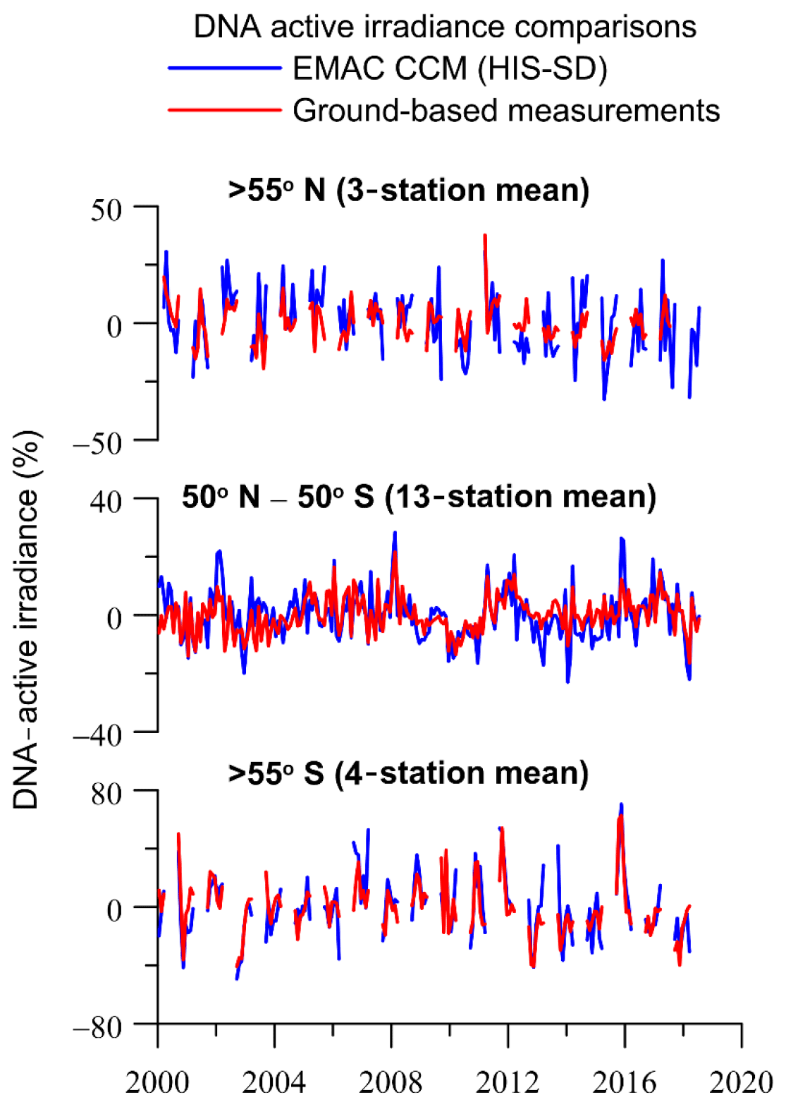
Figure 1Comparison of model simulations of DNA-active irradiance with averages of ground-based measurements at 3 UV stations in the northern high latitudes (> 55∘ N) (upper panel), 13 UV stations from 50∘ N to 50∘ S (middle panel), and 4 UV stations in the southern high latitudes (> 55∘ S) (lower panel). The y axis shows monthly de-seasonalized DNA-active irradiance data (in %). The monthly data at each station were de-seasonalized by subtracting the long-term monthly mean (2000–2018) pertaining to the same calendar month and were expressed in percent. Then, the average over each geographical zone was estimated by averaging the de-seasonalized data of the stations belonging to each geographical zone. Shown are data from March to September for the northern high latitudes and from September to March for the southern high latitudes.
2.4 Statistical methods
In Sect. 3.1, we evaluate the variability in DNA-active irradiance from the model simulations with station measurements for a nearly 20-year period (2000–2018). The comparisons were based on regression analyses between the simulated and the observed DNA-active irradiance monthly data after removing variations related to the seasonal cycle. The monthly data at each station were de-seasonalized by subtracting the long-term monthly mean (2000–2018) pertaining to the same calendar month.
We have calculated the Pearson's correlation coefficients, R, between the simulated and measured DNA-active irradiance (Eq. 1) and tested it for statistical significance using the t test formula for the correlation coefficient with n 2 degrees of freedom (Eq. 2) (von Storch and Zwiers, 1999):
where x refers to the measured and y to the simulated data.
The same procedure was followed for the comparisons between the simulated and satellite-derived total-ozone and cloud cover datasets for the period 2000–2018, which are presented in Sect. 3.1.
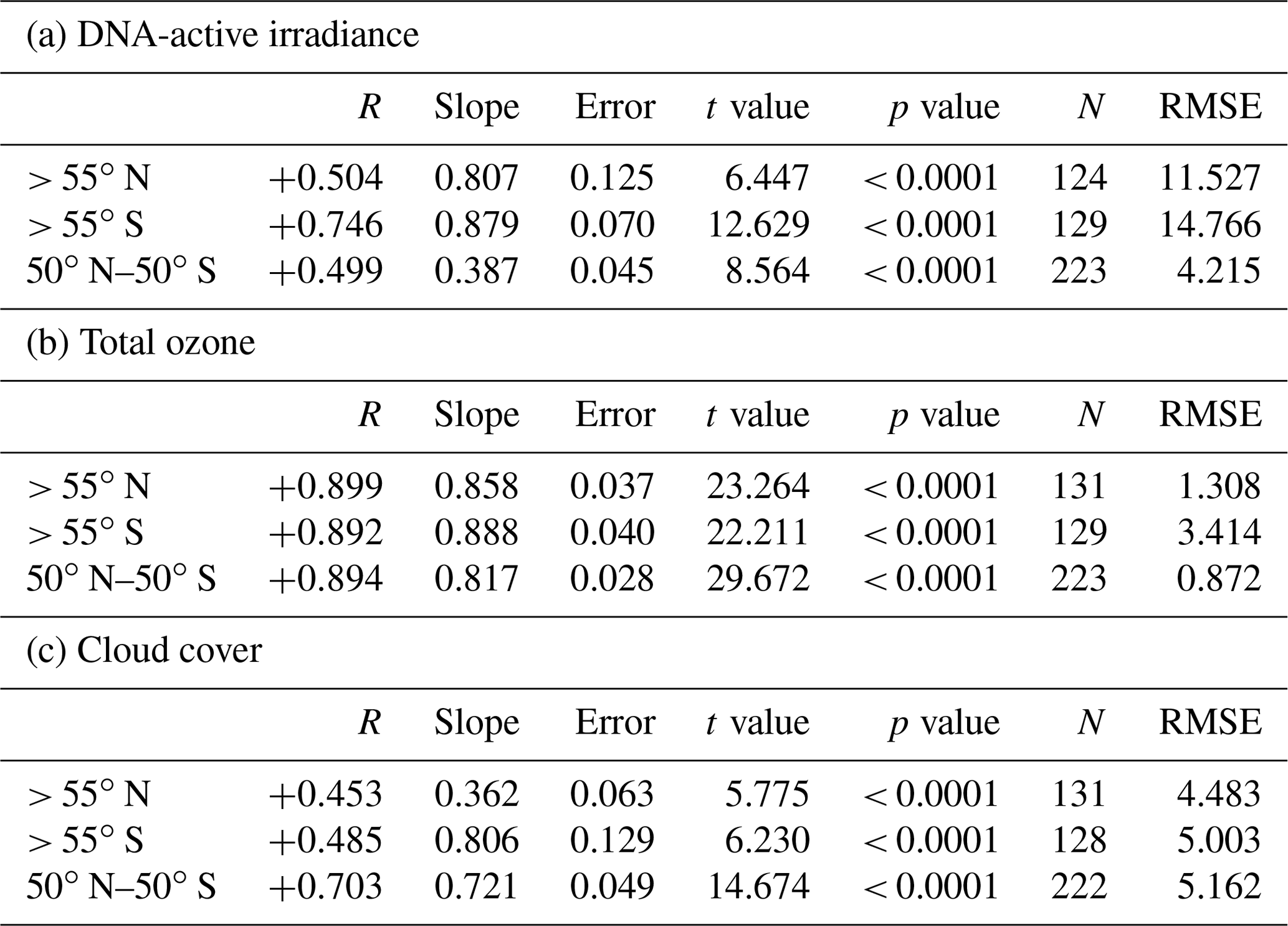
Table 2(a) Correlation results between model simulations (HIS-SD) and ground-based DNA-active irradiance data for the northern high-latitude stations (> 55∘ N), the southern high-latitude stations (> 55∘ S), and the stations between 50∘ N–50∘ S. (b) Same as (a) but for the HIS-SD simulation and satellite SBUV (v8.7) total-ozone data. (c) Same as (a) but for the HIS-SD simulation and satellite MODIS Terra cloud fraction data. Error, t value, and p value refer to slope; t value should be higher than 2.576 for 99 % statistical significance.
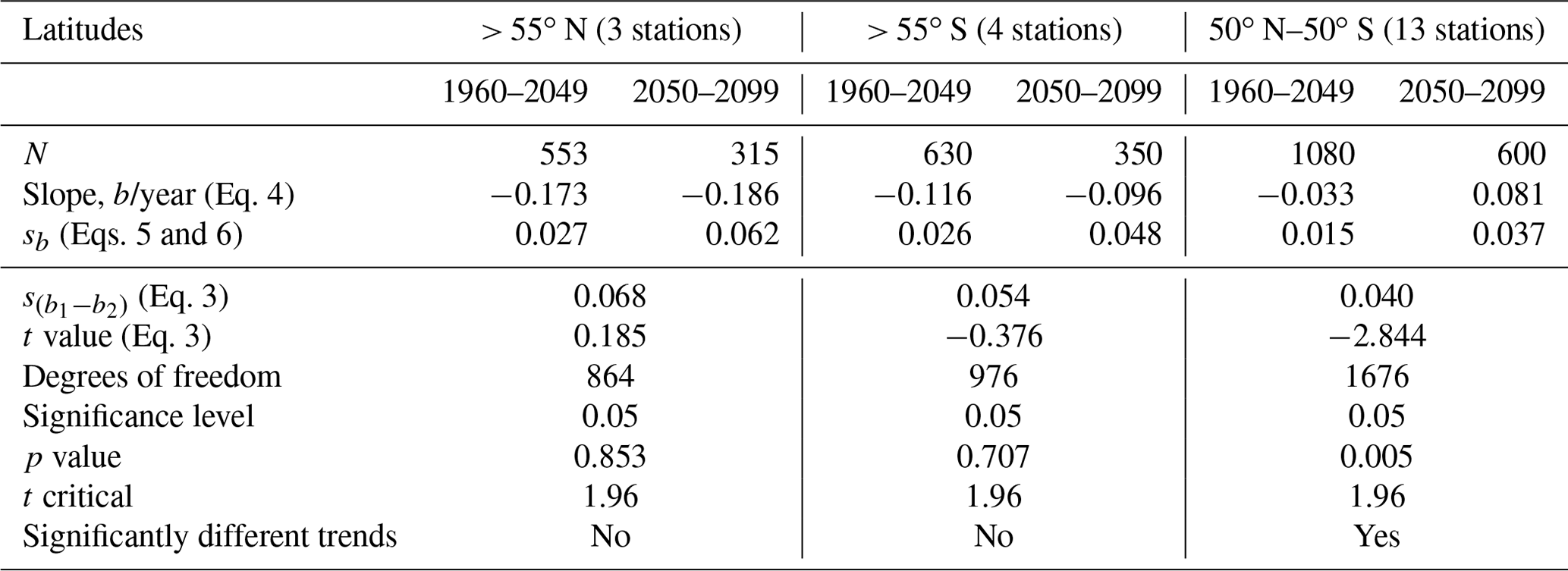
In Sect. 3.3, we apply a statistical test to compare the regression slopes in DNA-active irradiances before and after the year 2050. The null hypothesis that the two slopes are statistically equal ( is tested against the alternative hypothesis that the two slopes are not statistically equal (. The difference in slopes is tested with the following statistic:
with degrees of freedom, according to Eq. (11.20) of Armitage et al. (2001). The parameter is the standard error of The parameters b1 and b2 are the slopes before and after 2050 in each geographical zone, and n1 and n2 are the numbers of data before and after 2050, respectively. The test was performed using de-seasonalized monthly values but also with the averages shown in Figs. 4c, 5c, and 6c, calculated from de-seasonalized data. Both gave similar statistical results. In Sect. 3.3 we present the results using the de-seasonalized monthly values.
The slope of the regression line, where x is the time variable and y is the DNA-active irradiance, is given by
The residual mean square for the first group (1960–2049), , is given by
and the corresponding mean square for the second group (2050–2099), , by
Here, Syy is the standard deviation of DNA-active irradiance, Sxx is the standard deviation of time, and Sxy is their covariance, for the first (1960–2049) and second (2050–2099) periods.
If , then the null hypothesis H0 (the slopes are equal) is rejected at the significance level a and the alternative hypothesis (the two slopes are statistically different) is accepted.
3.1 Evaluation of EMAC CCM simulations for the present
The time series of de-seasonalized DNA-active irradiance data are presented in Fig. 1. The figure compares model calculations of DNA-active irradiance from the HIS-SD simulation with ground-based measurements at stations described in Sect. 2. The upper panel refers to the average of de-seasonalized data at three stations in the northern high latitudes, the middle panel refers to the respective average of 13 stations between 50∘ N and 50∘ S, and the lower panel to the respective average of four stations in the southern high latitudes. The comparisons refer to the period 2000–2018. We note that this is a composite dataset, obtained with the same set of stations (both in the model and in the observations). All time series in the model start from the same year but not in the observations.
The analysis shows that the correlations between the simulated and ground-based DNA-active irradiance data are statistically significant. Figure 1, however, shows that the variability between the simulated and ground-based data can be different. This becomes evident from Fig. 2 which presents the respective scatter plots. We have added the linear regression line and the y=x line, which shows how much the slope of the fit deviates from the 1:1 line. The statistical results (correlation coefficient, slope, error, t value, p value, and root mean square error (RMSE)) are summarized in Table 2a.
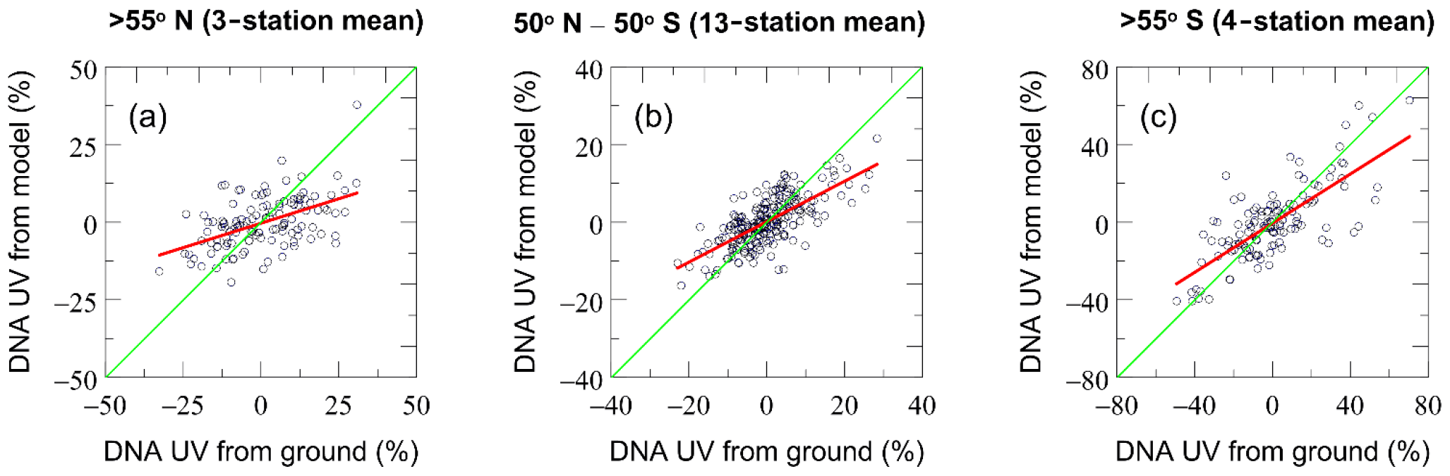
Figure 2Scatter plots of DNA-active irradiance from simulated and ground-based data shown in Fig. 1 for (a) 3 UV stations in the northern high latitudes (> 55∘ N), (b) 13 UV stations from 50∘ N to 50∘ S, and (c) 4 UV stations in the southern high latitudes (> 55∘ S).
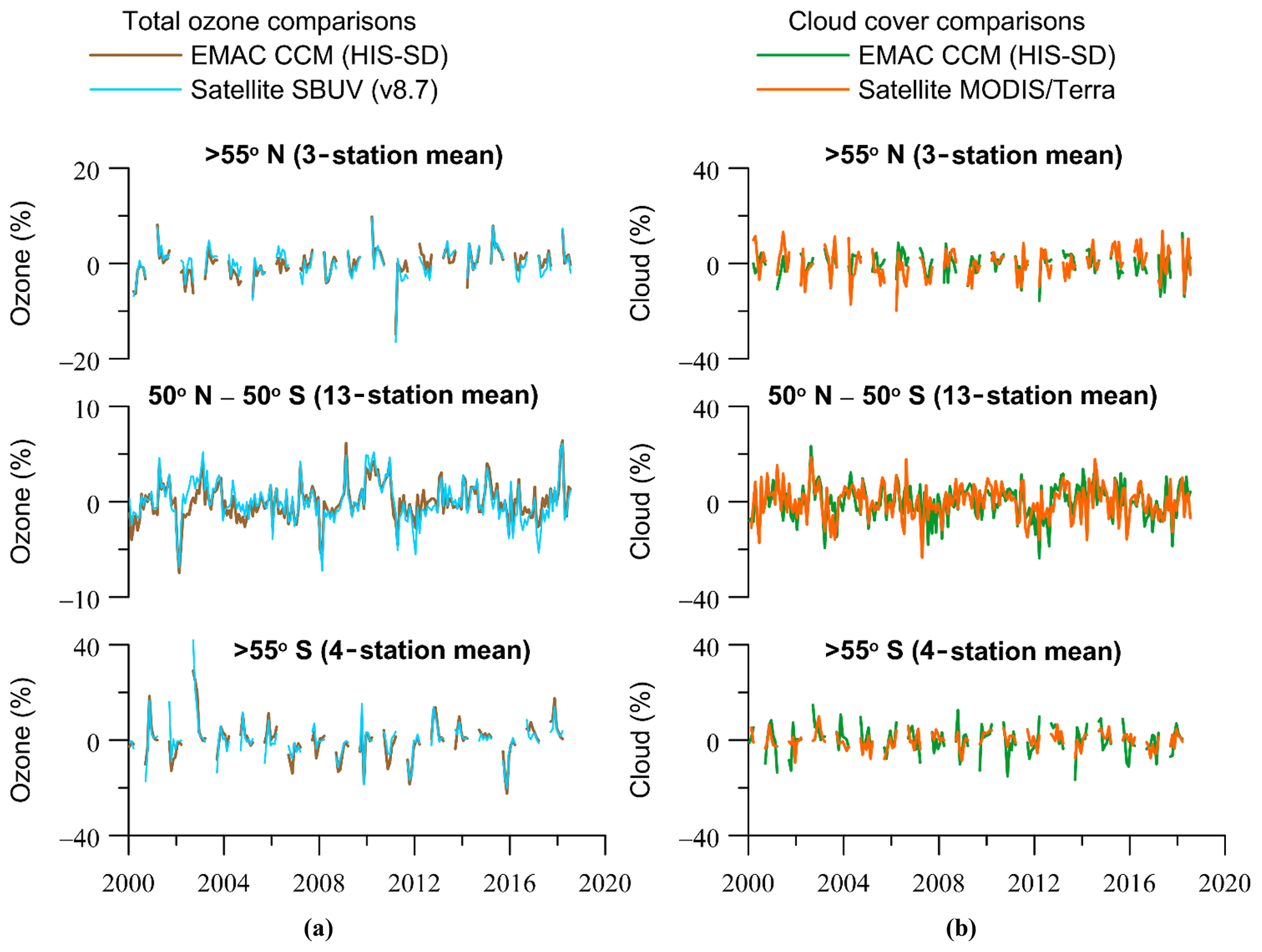
Figure 3(a) Same as in Fig. 1 but for ozone column. (b) For cloud cover. The y axes show monthly de-seasonalized anomalies (in %) relative to the long-term monthly mean (2000–2018). Shown are monthly anomalies from March to September for the northern high latitudes and from September to March for the southern high latitudes. For 50∘ N–50∘ S, we present all months.
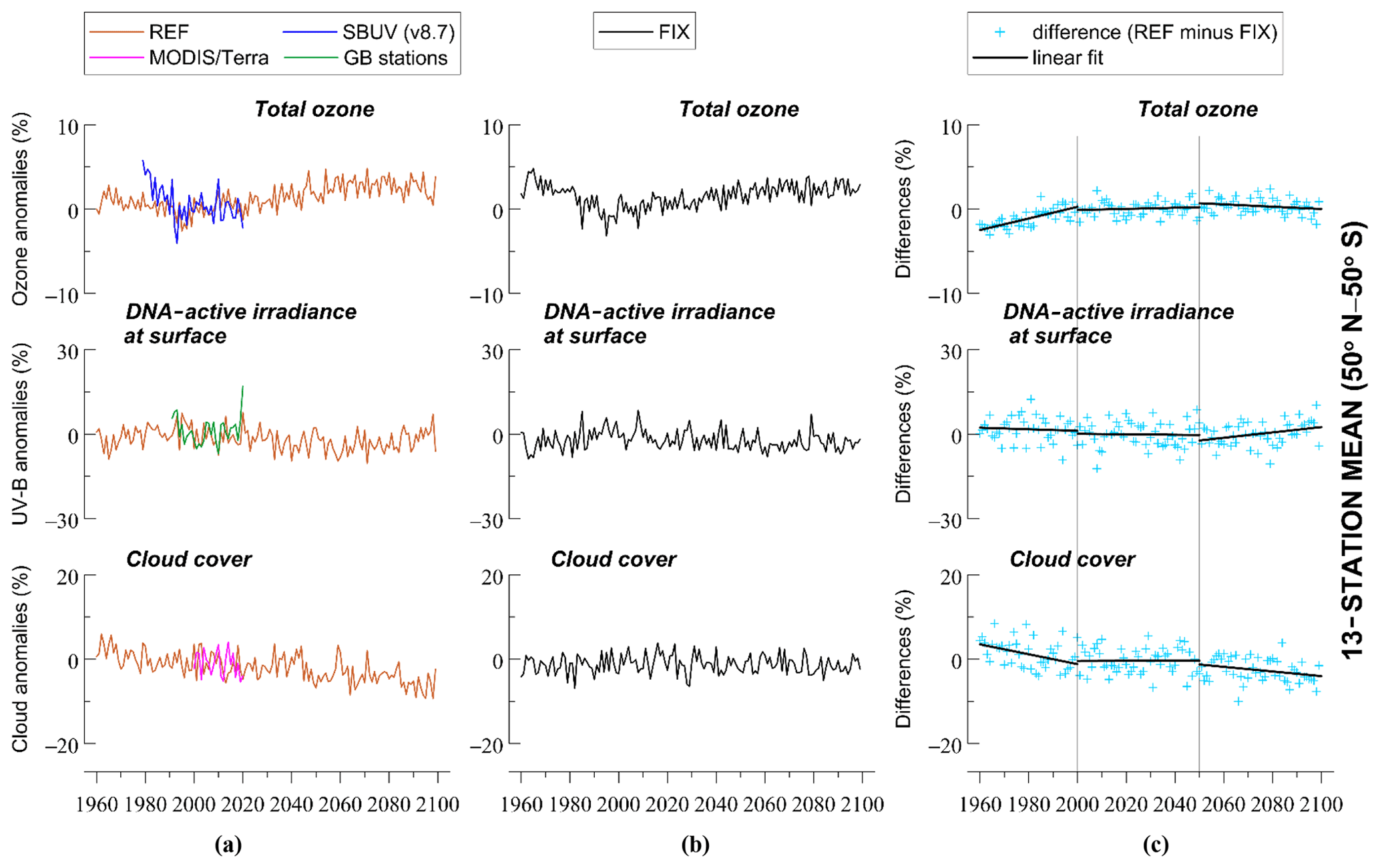
Figure 4Changes in total ozone, DNA-active irradiance, and cloud cover averaged at 13 UV stations from 50∘ N to 50∘ S, based on simulations with increasing and fixed-GHG mixing ratios. (a) REF is the simulation with increasing GHGs according to RCP 6.0. (b) FIX is the simulation with fixed-GHG emissions at 1960 levels. (c) Difference between the two model simulations, indicating the impact of increasing GHGs. The y axes in (a) and (b) show yearly averaged data (in %) calculated from de-seasonalized monthly data. The monthly data were de-seasonalized relative to the long-term monthly mean (1990–2019) and were expressed in percent. For stations between 50∘ N–50∘ S we used all months to calculate the annual average.
For the near-global mean, the correlation coefficient between the simulated and observed DNA-active irradiances is +0.709, the slope of the fit is 0.521, its error is 0.035, and the RMSE is 4.423. For the northern high latitudes, the statistical results are R=0.518, slope = 0.657, error of slope = 0.129, and RMSE = 9.543, while for the southern high latitudes they are R=0.746, slope = 0.879, error of slope = 0.070, and RMSE = 14.766. It appears that the slope of the regression fit for the near-global mean is small; however, the RMSE, which is the measure of the differences between the simulated and observed values, is also small. An RMSE of 0 would indicate a perfect fit to the data, something that is never achieved in practice. It also appears that the respective RMSE of the residuals (i.e. the simulated minus observed values) are larger at high latitudes; this is because it was derived from larger differences in de-seasonalized data at the northern high latitudes and even larger differences at the southern high latitudes.
The regression analysis results between the two datasets at each station separately are presented in Table S1. We note here that the model has a resolution of 2.8∘ × 2.8∘, which is a large area to be represented by point measurements. As such, for stations with inhomogeneous surrounding area, such as mountain tops (Mauna Loa, Sonnblick, Zugspitze), valleys (Aosta), or in towns with very heterogeneous surroundings (sea, mountains) and atmospheric conditions (tropospheric ozone and aerosols), like Athens, the model simulations of DNA-active irradiance are not expected to fully agree with the measurements. Thus at some stations, the correlation between simulated and measured DNA-weighted UV irradiance is not very good, as shown in the Supplement figures. For the same reason, the slope between the two datasets can deviate significantly from unity (see Table S1). Therefore, the comparisons at the individual stations provide a qualitative evaluation of the model's variability but cannot be regarded as a strict validation of the model. We provide here indicative estimates for individual stations, which give very good to excellent correlations: (a) Summit, Greenland – , slope = 0.757, error of slope = 0.081, p value < 0.0001, N=88; (b) Hoher Sonnblick, Austria – , slope = 0.946, error of slope = 0.075, p value < 0.0001, N=192; (c) Boulder, CO, USA – , slope = 0.677, error of slope = 0.047, p value < 0.0001, N=163; (d) Arrival Heights, Antarctica – , slope = 1.000, error of slope = 0.033, p value < 0.0001, N=126.
The same procedure was followed to evaluate simulated ozone and cloud cover. Figure 3 shows (a) ozone calculations from the HIS-SD simulation compared to satellite SBUV retrievals and (b) shows simulated cloud cover compared to cloud cover from MODIS Terra. It appears that the variability in ozone from the model simulation follows the variability in ozone from the satellite retrievals exceptionally well. It also appears that the variability in cloud cover from the model simulation is quite well correlated with the variability from the satellite observations (see Table 2b and c). The respective comparisons using zonally averaged data for the northern high latitudes (55–75∘ N), the near-global mean (50∘ N–50∘ S), and the southern high latitudes (55–75∘ S) are presented in Fig. S1. The regression results (R, slope, error of slope, t value, p value, and RMSE) for the large-scale latitudinal averages are presented in Table S2, and they are in line with the results from the station averages.
Table S3 presents the comparisons of total ozone between the EMAC CCM calculations and SBUV satellite retrievals analytically. The correlations between the two different datasets are statistically significant at a confidence level greater than 99.9 % at all stations under study. The correlation results for four indicative stations are as follows: (a) Summit, Greenland – , slope = 0.791, error of slope = 0.028, p value < 0.0001, N=131; (b) Hoher Sonnblick, Austria – , slope = 0.803, error of slope = 0.026, p value < 0.0001, N=223; (c) Boulder, CO, USA – , slope = 0.757, error of slope = 0.031, p value < 0.0001, N=223; (d) Arrival Heights, Antarctica – , slope = 0.655, error of slope = 0.029, p value < 0.0001, N=128.
Table S4 presents the respective comparisons for cloud cover. The cloud observations come from MODIS Terra. The correlation results for these four stations are as follows: (a) Summit, Greenland – , slope = 0.069, error of slope = 0.031, p value = 0.025, N=131; (b) Hoher Sonnblick, Austria – , slope = 0.619, error of slope = 0.062, p value < 0.0001, N=222; (c) Boulder, CO, USA – , slope = 0.482, error of slope = 0.051, p value < 0.0001, N=222; (d) Arrival Heights, Antarctica – , slope = 0.949, error of slope = 0.133, p value < 0.0001, N=129.
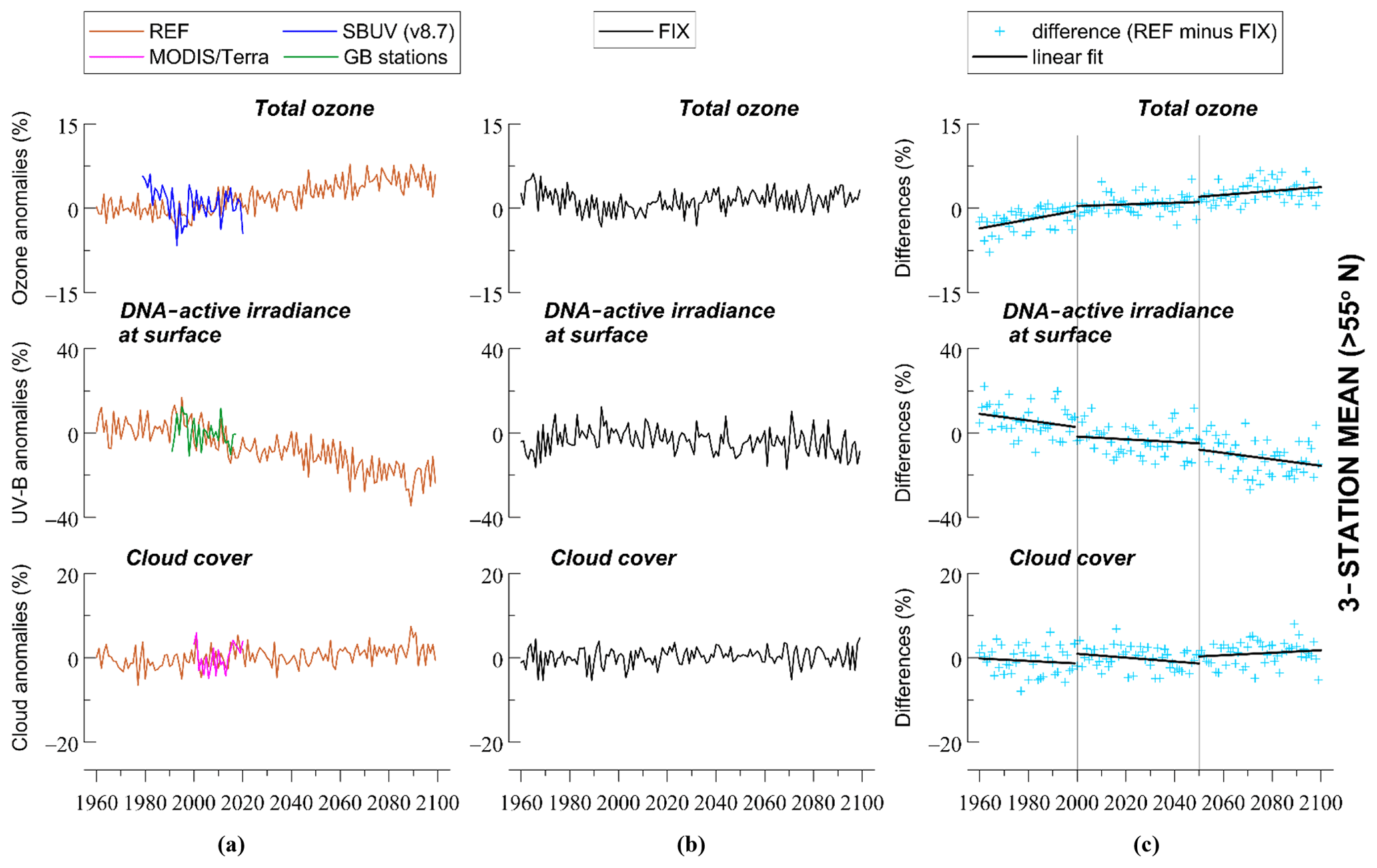
Figure 5Same as Fig. 4 but for three UV stations in the northern high latitudes (> 55∘ N). The y axes in (a) and (b) show averages of monthly de-seasonalized anomalies from March to September.
3.2 Future changes in ozone and DNA-active irradiance
In the previous section we evaluated the SD simulation SC1SD-base-02 with satellite and ground-based measurements. In this section we use the EMAC CCM simulations to investigate the evolution of DNA-active irradiance and the parameters that affect its long-term variability in the future. More specifically, we have analysed the free-running simulation of the EMAC CCM, namely RC2-base-04, with increasing GHGs according to RCP 6.0 at the stations under study. An evaluation of the free-running simulation RC2-base-04 with the SD simulation SC1SD-base-02 is provided in Appendix A. It helps to evaluate the quality of the results of the free-running model system with respect to the SD simulation and the observations of the stations, and it serves as a “bridge” from the observations via the SD simulation results to the results of the (longer-term) free-running model simulation.
We followed the same methodology as Eleftheratos et al. (2020), to examine the effect of increasing GHGs on the evolution of DNA-active radiation. We have compared the free-running simulation RC2-base-04 with the sensitivity simulation SC2-fGHG-01 where GHGs are kept constant at 1960 levels (see also Appendix A). The difference between the two free-running simulations gives us an estimate of the desired result.
We have prepared a series of figures to demonstrate the two different simulations and the differences between them. Figure 4 is based on 13 UV stations between 50∘ N and S. Figure 5 shows the results for the northern high-latitude stations and Fig. 6 for the southern high-latitude stations. The top panels refer to the evolution of total-ozone anomalies from 1960 to 2100; the middle panels refer to the evolution of DNA-active irradiance and the lower panels to the evolution of clouds for the same period. Panel a shows the two simulations, i.e. the free-running simulation with increasing GHGs (REF) versus the same simulation with fixed GHGs at 1960 levels (FIX), and panel b shows their respective differences. Shown are annual averages calculated from monthly de-seasonalized data. The calculation of annual averages was done as follows: first, we de-seasonalized the monthly data at each station by subtracting the long-term monthly mean (1990–2019) pertaining to the same calendar month. Next, we calculated a monthly de-seasonalized time series for each geographical zone by averaging the monthly de-seasonalized data of the stations belonging to each geographical zone. The latter time series was used to estimate the annual data anomalies. For the northern high-latitude stations, the annual average refers to the average of monthly anomalies from March to September, and for the southern high-latitude stations, it refers to the average of monthly anomalies from September to March. For the stations between 50∘ N–50∘ S we used all months to calculate the annual average.
In addition, we have added the DNA-weighted UV irradiance anomalies with green squares averaged at the ground-based stations under study around local noon. We also include the total-ozone anomalies from SBUV with blue dots and the respective cloud cover anomalies from MODIS Terra (magenta triangles) averaged at the stations studied. The observational data have been added to show simply that the dispersion of the simulated data matches the dispersion of the measured data.
In the study by Eleftheratos et al. (2020) data from five stations between 50∘ N and 50∘ S were analysed. Here, we examine 13 stations instead of 5 (Fig. 4) for this latitude band. The new findings paint the same picture: an increasing trend in DNA-active irradiance after the year 2050, associated with a decreasing trend in cloud cover due to the evolution of GHGs and a negative trend in total ozone (Fig. 4c). Thus, our new results, based on 13 instead of 5 stations, qualitatively confirm the results of the previous study for 50∘ N–50∘ S. An offset between total ozone from SBUV and the free-running simulation is evident in the 1980s, which is larger at 50∘ N–50∘ S. This is discussed later.

Figure 6Same as Fig. 4 but for four UV stations in the southern high latitudes (> 55∘ S). The y axes in (a) and (b) show averages of monthly de-seasonalized anomalies from September to March.
The focus now is at higher latitudes, which show a different picture than that of 50∘ N–50∘ S after the year 2050. At the northern high-latitude stations (Fig. 5), DNA-active irradiance (during the summer half year) shows a decreasing trend after 2050, total ozone shows an increasing trend after 2050, and cloud cover does not show any obvious statistically significant trend. The estimated trends (in % per decade) and their standard errors are presented in Table 3. More specifically, we estimate that total ozone will increase by 1.8 % ± 0.8 % from 2050 to 2100 (t value = 2.169, p value = 0.035), DNA-active irradiance will decrease by 8.2 ± 3.8% (t value 2.161, p value = 0.036), and cloud cover will slightly increase by 1.4 % ± 1.3 % (t value = 1.061, p value = 0.294). Accordingly, at the southern high-latitude stations (Fig. 6), total ozone is estimated to increase by 4.2 % ± 2.1 % from 2050 to 2100 (t value = 2.020, p value = 0.049), DNA-active irradiance is estimated to decrease by 4.8 % ± 2.9 % (t value 1.660, p value = 0.103), and cloud cover will decrease insignificantly by 1.1 %±1.7 % (t value , p value = 0.548).
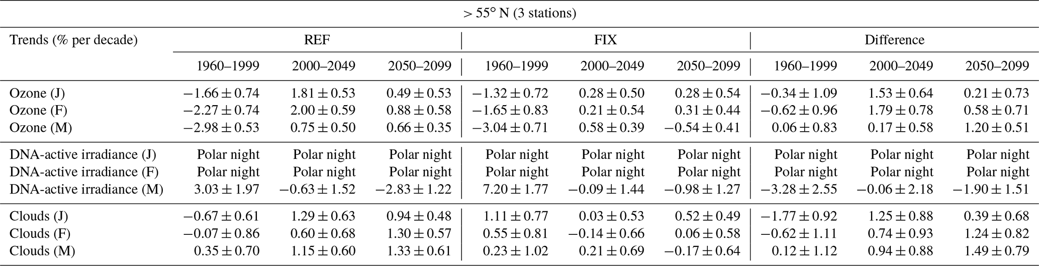
The above estimates point to an increase in total ozone in the northern high latitudes by the end of the century on an almost year-round basis. In a recent study by von der Gathen et al. (2021), it was concluded that conditions favourable for large Arctic ozone loss during cold winters could persist or even worsen by the end of this century if future abundances of GHGs continue to rise. As such, anthropogenic climate change has the potential to partially counteract the positive effects of the Montreal Protocol in protecting the Arctic ozone layer (von der Gathen et al., 2021). We examined the EMAC CCM projections regarding this finding. We have analysed the REF and FIX simulation results of ozone, DNA-active irradiance, and cloud cover for January, February, and March for the three northern high-latitude stations: Summit, Barrow, and Sodankylä. The trend results are presented in Table 4, which shows the trends from the two simulations and their differences for the periods 1960–1999, 2000–2049, and 2050–2099.
It appears that in January and February, regarded as the 2 coldest months of the year, the trends decrease from the first (2000–2049) to the second period (2050–2099), while in March (less cold month) the picture is different. More specifically, in January, the significant positive trend of 1.53 % ± 0.64 % per decade in 2000–2049 changes to 0.21 % ± 0.73 % per decade in 2050–2099. In February, the significant positive trend of 1.79 % ± 0.78% per decade in 2000–2049 decreases to 0.58 % ± 0.71% per decade in 2050–2099. On the other hand, the trends in March are 0.17 % ± 0.58 % per decade in 2000–2049 and 1.20 % ± 0.51% per decade in 2050–2099, and they agree with the general course of trends seen in Fig. 5. We end up with findings that are qualitatively in agreement with those of von der Gathen et al. (2021) about the large seasonal losses of Arctic ozone during cold winters by the end of the century. We also attempted to estimate the trends in DNA-active irradiance in the northern high-latitude stations for January, February, and March. The results are presented in Table 4 for the two periods – 2000–2049 and 2050–2099 – but due to the polar night at the northern high latitudes, UV values are very low in January and February, and the predicted trends have large standard errors. As such, they are not analysed any further.
Another issue is that Fig. 5a suggests that clouds will stay more or less constant over the Arctic. Other models predict that cloud cover in the Arctic will increase by the end of the century. With sea ice diminishing in the Arctic, evaporation would increase, leading to more moisture in the air, resulting in more clouds, which in turn is expected to reduce UV radiation. For example, Fountoulakis and Bais (2015) analysed changes in UV radiation projected for the Arctic. Comparison of Fig. 1 (clear-sky trends) and Fig. 2 (all-sky trends) of Fountoulakis and Bais (2015) suggests that UV changes between the future and the present will become more negative when clouds are also considered due to the projected increase in cloud attenuation. Our estimates indicate a significant cloud increase of ∼2.2 % from 1960 to 2100 (∼1.4 % from 2050 to 2100, not significant). These increases are small and are based on the average of three stations only – Summit, Barrow, and Sodankylä – but they are in accordance with the results obtained for the whole latitudinal band of 55–75∘ N (∼2.7 % from 1960 to 2100, p value < 0.0001, and ∼0.9 % from 2050 to 2100, p value = 0.05). Summit and Sodankylä are far away from the seashore and are not affected by the ocean, while Barrow is located only 250 m away from the coast and is greatly affected by the ocean. Changes in cloudiness might be different at coastal and mainland sites. For Barrow (coastal site) we estimate a significant cloud increase of 5.5 % in the period 1960–2100 (3 % in the period 2050–2099), while for Summit (pure land site) we estimate an insignificant change of −0.1 % in the period 1960–2100 (−0.4 % in the period 2050–2100). For Sodankylä (also pure land site), we estimate an insignificant increase of 1.2 % in the period 1960–2100 (p value = 0.365) and of 1.6 % in the period 2050–2100 (p value = 0.446). Averaging large and small changes in cloudiness should finally result in moderate changes. These results generally agree with the results presented in other studies (Bais et al., 2015; Fountoulakis and Bais, 2015) for land areas of the Arctic (keeping also in mind that the results of the present study are averages for three stations only). We note that the results presented in these two referenced studies were for RCPs 4.5 and 8.5 and thus not directly comparable with the results of our study. In a more recent study presenting RCP 6.0-based projections (Bais et al., 2019), it was shown that cloudiness changes at high latitudes would strongly affect the UV irradiance mainly over the ocean where the absence of sea ice would result in increased evaporation. For land, smaller and non-significant changes were reported (see Fig. 8 of Bais et al., 2019), which is again in agreement with the results presented in our study. In another study (Fig. 5 of Fountoulakis et al., 2014), changes in zonally averaged UV irradiance due to changes in cloudiness in 1950–2100 were estimated to be on the order of 5 %–15 % (depending on the RCP) for latitudes ∼70degree. However, only changes over the ocean were considered in that study and not over land. Additional indications that our results should be considered representative of the three stations under study and not the entire Arctic region is provided in Fig. B1 (Appendix B), which shows the changes in zonal mean cloud cover for the Arctic region from the REF simulation. It appears that the zonal mean cloudiness is expected to increase more and more as it moves northward of 50∘ towards the North Pole, indicating that the largest changes in cloud cover are likely to occur over the ocean and not over land.

Figure 7(a) Changes in surface albedo at Barrow, Alaska, and (b) at Palmer, Antarctica, derived from the differences between the two model simulations: the one with increasing GHGs (REF) and the one with fixed GHGs (FIX). Results refer to the summer season. Data were de-seasonalized with respect to the period 1990–2019 and then were averaged from March to September at Barrow and from September to March at Palmer. The left y axis shows the differences in surface albedo values and the right y axis shows the respective differences in percent of the mean.
Table 3Trends (% per decade) in total ozone, DNA-active irradiance, and cloudiness from the two model simulations and the differences between them, i.e. free-running simulation with increasing GHGs (REF) minus the simulation with fixed GHGs at 1960 levels (FIX), averaged at 3 stations in the northern high latitudes (> 55∘ N), 4 stations in the southern high latitudes (> 55∘ S), and 13 stations between 50∘ N–50∘ S. The trends are estimated from the annual mean anomalies shown in Figs. 4, 5, and 6.
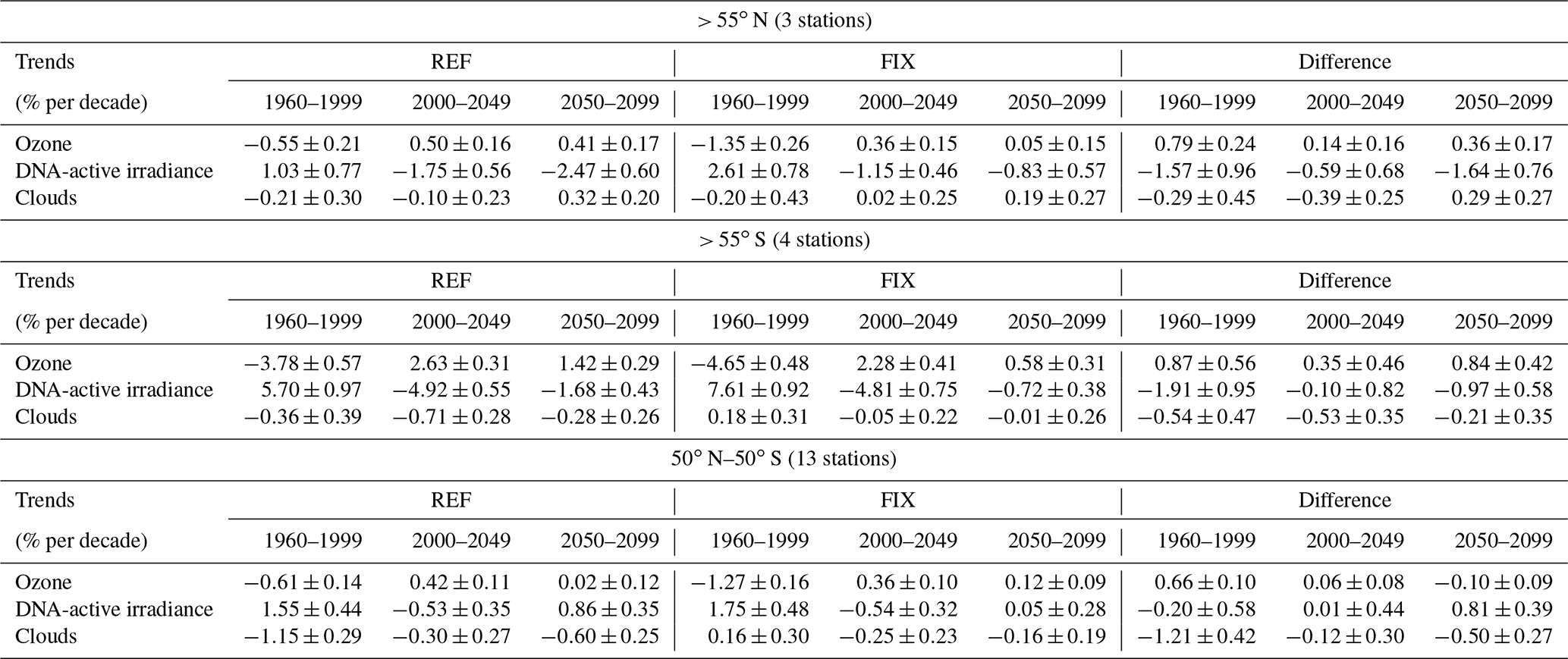
Table 4Same as Table 3 but for the winter months, January (J), February (F), and March (M) for the northern high-latitude stations. Due to the polar night, UV results for January and February are not shown due to large standard errors.
For the period 1960–1999, the DNA-active irradiance (summer half year) showed upward trends in all geographical zones following the downward trends of total ozone. Nevertheless, we should note that the examined simulation REF (simulation with full chemistry and increasing GHGs according to RCP 6.0) seems to clearly underestimate the observed ozone depletion of the 1980s and 1990s in the geographical region 50∘ N–50∘ S (Fig. 4), but in the higher latitude regions (Figs. 5 and 6) the picture looks much better. This suggests that there may be a bias in the model that might at least partly be caused by not considering all ozone-depleting substances (ODSs) but only a subset (only CFC-11 and CFC-12 are considered; Jöckel et al., 2016). The REF simulation also underestimates the ozone depletion of the 1980s and 1990s in the northern high-latitude stations (Fig. 5), but the picture is better than that of 50∘ N–50∘ S. The FIX simulation seems to reproduce the Arctic ozone depletion of the past better. The latter, however, is coincidence; it only indicates that due to the higher dynamic variability in the northern (winter) stratosphere, the evolution of the ozone layer in the Arctic region is significantly affected by natural variability in the stratosphere due to planetary waves. The best agreement between the REF simulation and satellite measurements during the period of ozone depletion is found for the southern high latitudes, as can be seen from Fig. 6. As such, we can infer that the model simulations reproduce the observed ozone depletion of the past very well in particular in the southern higher latitudes and less well in the northern higher latitudes. Nevertheless, the simulated decline in ozone during 1979–1999, and the minimum ozone values calculated by the model in the 1990s for the near-global mean (50∘ N–50∘ S) and for the higher latitudes are qualitatively in line with the satellite ozone observations, which is a good outcome. This is supported by Fig. A1 (Appendix A), which shows the free-running simulation REF against the SD simulation HIS-SD which starts in 2000. Because we wanted to evaluate the free-running simulation for the period of ozone depletion, we also analysed the SD simulation RC1SD-base-10, which starts in 1979. It appears that the REF simulation seems to reproduce the negative ozone trends well during the period of ozone depletion but not the exact anomalies of a particular year. This is because the free-running simulation has its own meteorological/synoptical sequence, and thus we cannot expect that the observed time series of the past is reproduced on a year-by-year basis in the free-running simulation the same way it is reproduced in the simulation with specified dynamics.
Finally, we should also refer to the recent assessment of the United Nations Environment Programme (UNEP) Environmental Assessment Panel (EEAP) (Bernhard et al., 2020), which compared projections of future UV radiation from two studies: Bais et al. (2019) and Lamy et al. (2019). We have compared our trend estimates, which are based on one model only, with the estimates provided in Table 1 of Bernhard et al. (2020), which are based on many models of the first phase of the Chemistry-Climate Model Initiative (CCMI-1) and should therefore be considered more robust than the estimates provided here. We clarify that it is only a qualitative comparison as our trends are based on DNA-weighted irradiance, while the table in Bernhard et al. (2020) refers to erythema. The DNA radiation amplification factor is about 2.1, while that for erythema is 1.2, which suggests that we would expect differences in trends by roughly a factor of 1.75. We also note that the table of Bernhard et al. (2020) shows zonal mean changes in the clear-sky UV index, whereas we estimate changes in DNA-active irradiance based on station averages. Despite the inconsistencies in the radiation fields being compared, our trend estimates from the REF simulation based on RCP 6.0 are qualitatively in line with the results presented by Bernhard et al. (2020) for the case of RCP 6.0. We estimate a statistically significant decrease in DNA-active irradiance at the northern high-latitude stations for the period 2015 to 2090 of about −17 % (−16 % for the zonal mean 55–75∘ N). The numbers from Table 1 of Bernhard et al. (2020) for the northern high latitudes are −6 % for the annual mean clear-sky UV index for the period 2015 to 2090 and −3 %, −7 %, −5 %, and −4 % for January, April, July, and October, respectively. Our respective estimate for the southern high-latitude stations is about −24 % (−26 % for the zonal mean 55–75∘ S) and is also qualitatively in line with the negative trend estimates provided by Bernhard et al. (2020) for the southern high latitudes for the period 2015 to 2090 (−18 % for the annual mean clear-sky UV index and −8 %, −6 %, −6 % and −23 % for January, April, July, and October, respectively).
Table 5Statistical test results for the difference between two trends in DNA-active irradiance (trend of 1960–2049 minus trend of 2050–2099), for the northern high-latitude stations (> 55∘ N), the southern high-latitude stations (> 55∘ S), and the stations between 50∘ N–50∘ S.
The above estimates are based on station averages. We have complemented the analysis presented in Figs. 4, 5, and 6 with zonally averaged data in order to exploit the model results over the entire domain, for example in latitudinal bands, and not only to 20 locations. The Figs. S2, S3, and S4 show the changes from the free-running simulations REF, FIX, and their differences for the near-global mean and the northern and southern high latitudes based on latitudinal averages. It appears that the results from the analysis of averaging the model data in latitudinal bands are in the same direction as those of the station averages. More specifically, for the near-global mean we find similar results to those presented in Fig. 4 for the stations' mean but a stronger negative trend in total ozone after 2050, which together with the negative cloud trend drives the positive DNA-active irradiance trend after 2050. On the other hand, negative trends in total ozone and clouds after 2050 are not observed in the northern or the southern high-latitude belt.
We believe that the negative trends seen in the near-global mean after 2050 result from the ongoing increases in GHGs that will affect total ozone and clouds. It is well known that increasing GHG concentrations have led to tropospheric warming and stratospheric cooling over the last decades (Stocker et al., 2013; Zerefos et al., 2014). As a thermodynamic consequence, the troposphere has expanded and the height of the tropopause has increased (Santer et al., 2003). A recent study showed that the stratospheric layer has contracted substantially over the last decades due to increasing GHGs and will continue to contract under the RCP 6.0 scenario (Pisoft et al., 2021). Also, chemistry–climate and climate model projections show an acceleration of the Brewer–Dobson circulation in response to GHG increases (Butchart, 2014). These changes will not leave the ozone layer unaffected. Our model simulations for the near-global mean show a downward trend in total ozone after 2050, which will likely be shaped by the negative trend in the lower stratosphere due to increasing GHGs. For clouds, it has been shown that increasing GHGs are responsible for fewer clouds over the mid-latitudes (Norris et al., 2016) and for breaking up stratocumulus clouds into scattered clouds (Schneider et al., 2019). Our simulations show that clouds will decrease in response to increasing GHGs, which is consistent with the findings of these studies.
The results based on the zonally averaged data fully support the basic finding of the paper that DNA-active irradiance is expected to change differently at high latitudes than at a near-global scale after around 2050. It will continue to decline at high latitudes mainly due to stratospheric ozone recovery from the reduction in ODSs (cloud cover changes are not significant), while it is expected to increase on a near-global scale, affected by GHG-induced reductions in cloud cover and total ozone. This of course is an outcome that emerges from the simulations of a single climate–chemistry model, and as such, it may well turn out to be true or false. Verification of the results from other model simulations would be important, but also important is further investigation of the cloud changes from the model simulations and their verification with high-quality measurements. It is important to note that our free-running simulations were designed according to the definitions for the reference and sensitivity simulations provided by the IGAC (International Global Atmospheric Chemistry) and SPARC (Stratosphere–troposphere Processes And their Role in Climate) communities to address emerging science questions, improve process understanding, and support upcoming ozone and climate assessments (Eyring et al., 2013).
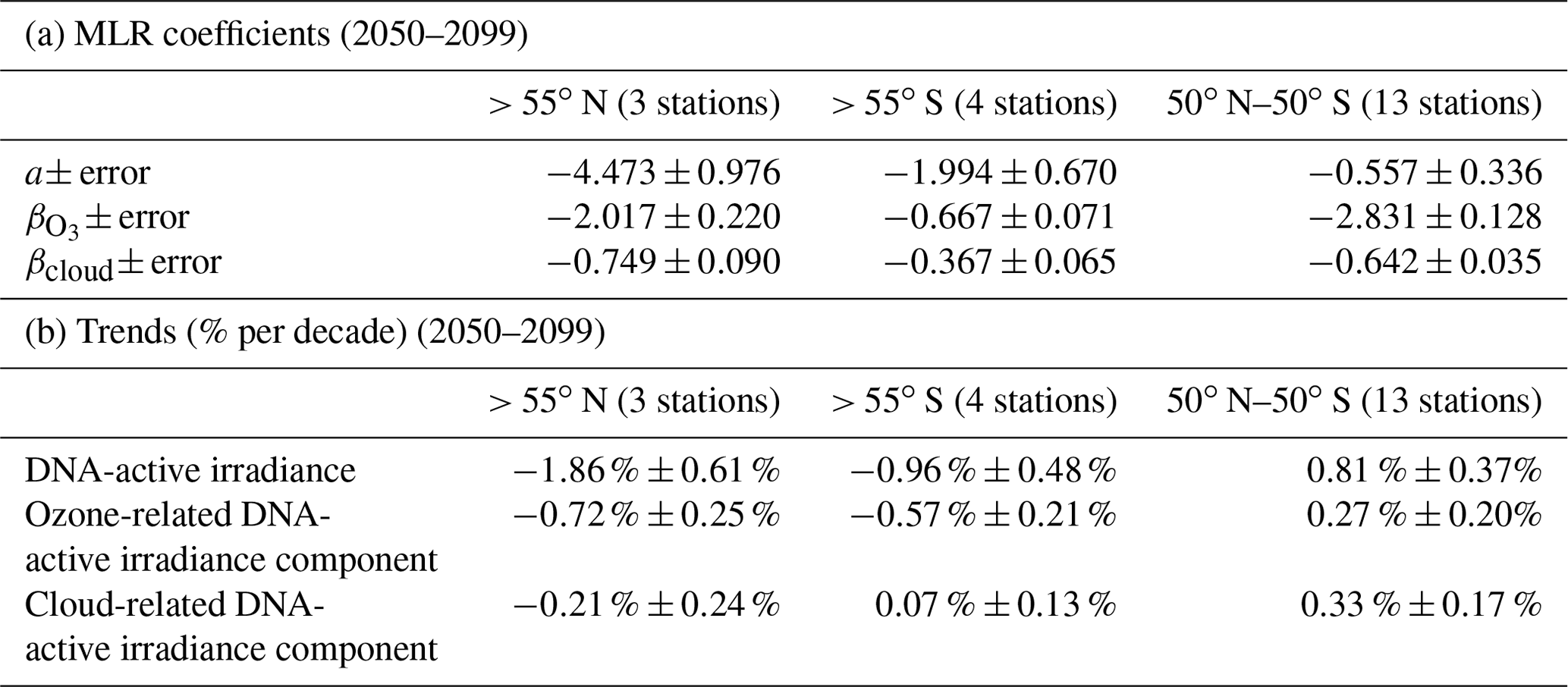
Table 6(a) Coefficients of multiple regression analysis according to Eq. (7), applied to the differences between the two model simulations – REF and FIX – for the period 2050–2099, for the northern high-latitude stations (> 55∘ N), the southern high-latitude stations (> 55∘ S), and the stations between 50∘ N–50∘ S. (b) Trends (% per decade) for the period 2050–2099 in the DNA-active irradiance, the ozone-related DNA-active irradiance component, and the cloud-related DNA-active irradiance component.
3.3 Statistical evaluation of differences between trends and statistical modelling
We have compared the regression slopes in DNA-active irradiances before and after the year 2050.
Our calculations according to Eq. (3) show that at the significance level α=0.05, the null hypothesis that the slopes are statistically equal cannot be rejected for neither the northern nor the southern high latitudes (> 55∘), and therefore we cannot conclude that there is any statistically significant difference between the trends in DNA-active irradiance before and after 2050 in these two latitude zones. On the other hand, the null hypothesis is rejected for the latitude zone of 50∘ N–50∘ S, which means that the alternative hypothesis is accepted, and so the two trends before and after 2050 are statistically different. The statistical results are presented in Table 5.
We note here that the statistical test was also applied for the periods before 2050, i.e. the two periods 1960–1999 and 2000–2049, to test if their trends are statistically significant or not. In all latitudes it was found that the regression slope of the period 1960–1999 is not statistically significantly different from the regression slope of the period 2000–2049. As such, it appears that only after the year 2050 there does appear to be a statistically significant change in the trends of DNA-active irradiance because of the evolution of GHGs and only at latitudes between 50∘ N and 50∘ S. At latitudes poleward of 55∘, the DNA-active irradiance is more likely to continue to decrease due to the increasing ozone trends from the reduction in the concentrations of ODSs.
Moreover, we have applied multiple linear regression (MLR) analysis to examine the contribution of ozone and cloud trends to the estimated DNA-active irradiance trends after the year 2050. The MLR model was applied to the differences between the two model simulations – REF and FIX – which were estimated from monthly de-seasonalized data (deseas). The MLR model is of the following form:
where a is the intercept, is the ozone coefficient and βcloud is the cloud coefficient for the period 2050–2099. The regression coefficients and their standard errors are presented in Table 6a. These coefficients were derived from station mean data and hence might not be representative of the entire geographical zones. As can be seen, the coefficients and βcloud are highly statistically significant with small errors in all cases (pvalues < 0.001). We have used the regression coefficients to determine the part of the DNA-active irradiance trends that are caused by trends in total ozone and cloud cover. We have derived the ozone-related DNA-active irradiance trend by multiplying the regression coefficient between DNA-active irradiance and ozone ( with the trend in ozone for the period 2050–2099. Accordingly, we derived the respective cloud-related DNA-active irradiance trend by multiplying the regression coefficient βcloud with the cloud trend.
Table 7Trends and their standard errors (% per decade) in the differences between the two model simulations – REF and FIX – for the DNA-active irradiance, total ozone, cloud cover, and surface albedo at Barrow (Alaska) and Palmer (Antarctica) for the periods 1960–1999, 2000–2049, and 2050–2099.

For the northern high-latitude stations (> 55∘ N), we estimate an ozone-related DNA-active irradiance trend of about −0.72 % per decade, indicating that ∼39 % of the DNA-active irradiance trend (−1.86 % per decade) is caused by the trends in ozone. The respective cloud-related DNA-active irradiance trend is smaller (−0.21 % per decade), which means that the cloud trend explains ∼11 % of the DNA-active irradiance trend. Both parameters account for ∼50 % of the predicted DNA-active irradiance trend. The remaining part of the DNA-active irradiance trend is related to changes in other parameters, as for instance in surface albedo, as is discussed later in Sect. 3.4.
Similar results regarding the contribution of ozone and cloud trends to the predicted DNA-active irradiance trend are also found for the southern high-latitude stations (> 55∘ S) but not for the stations averaged between 50∘ N and 50∘ S. The results are summarized in Table 6b. For the southern high-latitude stations (> 55∘ S), the ozone-related DNA-active irradiance trend is −0.57 % per decade and the cloud-related DNA-active irradiance trend is +0.07 % per decade. As such, ∼59 % of the DNA-active irradiance trend (−0.96 % per decade) is explained by ozone, and ∼7 % is explained by clouds.
For stations averaged between 50∘ N–50∘ S, we estimate that the ozone-related DNA-active irradiance trend is +0.27 % per decade, and the cloud-related DNA-active irradiance trend is +0.33 % per decade. The contribution of changes in cloudiness is larger than the contribution of changes in ozone (∼41 % compared to ∼33 %, respectively), and therefore, our findings support the previous results by Eleftheratos et al. (2020), who analysed a smaller number of GB stations between 50∘ N–50∘ S than those used here.
3.4 Changes in surface albedo and relation to DNA-active irradiance
In the previous section we showed that DNA-active irradiance will continue to decrease after the year 2050 at high latitudes as a result of ozone change rather than cloud cover change. Another parameter affecting the solar UV variability at high latitudes is surface albedo (Weihs et al., 1999; Nichol et al., 2003; Weatherhead et al., 2005; Gröbner, 2012; Bais et al., 2019). In this respect, changes in surface albedo are expected to affect the long-term variability in surface UV-B irradiance. Figure 6 shows the changes in surface albedo simulated with the EMAC CCM at the two stations: Barrow in Alaska and Palmer in Antarctica. More specifically the figure shows the differences between the two model simulations – the one with increasing GHGs (REF) and the one with fixed GHGs (FIX) – in order to account also for the effect of increasing GHGs on surface albedo changes according to the methodology applied in Sect. 3.2. The results refer to the summer seasons of the two hemispheres, where there is sufficient sunlight in the Arctic and the Antarctic. Table 7 summarizes the trends in the differences between the two model simulations – REF and FIX – for the DNA-active irradiance, total ozone, cloud cover, and surface albedo at Barrow (Alaska) and Palmer (Antarctica) for the periods 1960–1999, 2000–2049, and 2050–2099. While variations in surface albedo are certainly of primary importance for high-latitude sites, they can play a non-negligible role even at mid-latitudes. However, they were not analysed here.
From Fig. 7 it is clear that surface albedo decreases significantly by the end of the 21st century in view of the increasing GHG emissions. The decreases in surface albedo (Table 7) are larger in Barrow (Alaska) than Palmer (Antarctica). The trend for Barrow is qualitatively consistent with the conclusion by Bernhard (2011), showing that the ground at Barrow is covered by snow later and later at the start of winter. We also note that both Barrow and Palmer are coastal sites and are heavily affected by local conditions (e.g. how far sea ice gets to the station), which may not be simulated correctly. Therefore, we point out that the evolution of albedo at the two stations shown in Fig. 7 is representative of regional changes but may not accurately reflect changes at the exact location of these stations.
To assess the impact of the albedo changes on UV variability, we used surface albedo as additional explanatory variable in the MLR model of Eq. (7). We determined an additional regression coefficient, namely βalbedo, which explains the effect of albedo change on DNA-active irradiance change at the two stations under study: Barrow and Palmer. We estimated an albedo-related DNA-active irradiance trend, in the same way as described above, by multiplying the coefficient βalbedo with the trend in albedo differences between the two model simulations.
For Barrow, we estimate an ozone-related DNA-active irradiance trend of about −0.87 % per decade for the period 2050–2099, indicating that ∼41 % of the DNA-active irradiance trend (−2.14 % per decade) is caused by trends in ozone. The respective cloud-related DNA-active irradiance trend is about −0.49 % per decade, which means that the cloud trend explains ∼23 % of the DNA-active irradiance trend. The surface albedo-related DNA radiation trend is about −0.45 % per decade, explaining ∼21 % of the DNA-active irradiance trend in the period 2050–2099. The model suggests that all parameters together explain ∼85 % of the DNA-active irradiance trend, which however may not be such an unbiased result. This is because the effects of clouds and albedo are not independent, as assumed in the regression equation. For 100 % albedo and non-absorbing clouds, clouds would barely attenuate UV radiation. For actual albedo and cloud conditions, clouds do attenuate, but the effect is greatly reduced by surface albedo because of multiple reflections between surface and cloud (Nichol et al., 2003).
At Palmer, the trends are smaller. The ozone-related DNA-active irradiance trend is −0.46 % per decade, the cloud-related DNA-active irradiance trend is 0.43 % per decade, and the albedo-related DNA-active irradiance trend is −0.31 % per decade. These trends together determine the small negative trend which is predicted for the DNA-active UV irradiance in the period 2050–2099 of about −0.33 % per decade.
The above calculations indicate that the impact of albedo trends on DNA-active irradiance trends due to the continuous increase in GHGs until the end of the 21st century is important and should not be ignored when studying the long-term changes in DNA-active radiation reaching the ground. The model simulations at Barrow and Palmer suggest that the surface albedo changes might be larger at Barrow than Palmer according to Table 7. The model simulations also suggest that the northern high latitudes might experience larger changes in surface albedo than the southern high latitudes in the period 2050–2100 (Appendix C, Figs. C1 and C2).
In order to better represent the northern and southern high latitudes, we also applied the MLR model to the large-scale zonal means of 55–75∘ N and 55–75∘ S. For the northern high-latitude zone, the findings are in the same direction as those found for Barrow. We estimate that ∼31 % of the DNA-active irradiance trend is attributable to the trend in total ozone and that ∼14 % and ∼32 % of the DNA-active irradiance trend are explained by trends in clouds and surface albedo, respectively. For the southern high-latitude zone, we estimate that the largest part of the DNA-active irradiance trend is explained by the trend in total ozone and that the contributions of cloud and albedo trends are small.
We have studied changes in ozone, DNA-active irradiance and cloud cover due to the evolution of greenhouse gas concentrations in the near-global mean (50∘ N–50∘ S) and in the northern and southern high latitudes, using the EMAC CCM simulations from 1960 to 2100.
The model simulations have been evaluated against ground-based UV irradiance measurements, satellite ozone observations from SBUV (v8.7), and satellite cloud fraction data from MODIS Terra for the period 2000–2018. The evaluation results can be summarized as follows:
-
Simulations of total ozone with specified dynamics (RC1SD-base-10 and HIS-SD) reproduce the variability in total ozone extremely well in the northern and southern high latitudes for the periods 1979–2013 and 2000–2018, respectively. The correlation analysis results between EMAC HIS-SD simulation and SBUV (v8.7) satellite ozone de-seasonalized data are as follows: northern high latitudes (3-station mean) – , p value < 0.0001; southern high latitudes (4-station mean) – , p value < 0.0001; 50∘ N–50∘ S (13-station mean) – , p value < 0.0001.
-
The respective simulations of DNA-active irradiance correlate quite well with ground-based UV measurements, as follows: northern high latitudes (3-station mean) – , p value < 0.0001; southern high latitudes (4-station mean) – , p value < 0.0001; 50∘ N–50∘ S (13-station mean) – , p value < 0.0001.
-
Evaluation of cloud cover simulations against MODIS Terra cloud fraction data gave good correlations as follows: northern high latitudes (3-station mean) – , p value < 0.0001; southern high latitudes (4-station mean) – , p value < 0.0001; 50∘ N–50∘ S (13-station mean) – , p value < 0.0001.
Between 50∘ N–50∘ S, the DNA-damaging UV radiation is expected to decrease until 2050 and to increase thereafter. This increase is associated with expected decreases in cloud cover and insignificant trends in total ozone, as was shown previously by Eleftheratos et al. (2020). Our study however expands the previous work by adding more stations at low latitudes and mid-latitudes and by including estimates from high-latitude stations with long-term measurements of UV irradiance.
In contrast to the predictions for 50∘ N–50∘ S, we estimate that DNA-active irradiance will continue to decrease after the year 2050 in the northern and southern high latitudes (> 55∘) due to increasing ozone. More specifically, for the northern high-latitude stations we estimate that total ozone will increase by 1.8 % ± 0.8 % from 2050 to 2100, DNA-active irradiance will decrease by 8.2 % ± 3.8 %, and cloud cover will increase insignificantly by 1.4 % ± 1.3 %. Similarly, at the southern high-latitude stations, total ozone is estimated to increase by 4.2 % ± 2.1% from 2050 to 2100, DNA-active irradiance is estimated to decrease by 4.8 % ± 2.9%, and cloud cover will decrease insignificantly by 1.1 % ± 1.7%.
The statistical results have been confirmed by statistical tests. Statistical comparisons of the regression slopes before and after 2050 in the northern and southern high-latitude stations under study showed that there are no statistically significant different trends in DNA-active irradiance before and after that year. On the other hand, between 50∘ N–50∘ S the trends before and after 2050 were found to be statistically significantly different at the 0.05 significance level. The test confirmed the statistical result that DNA-active irradiance will reverse sign and become positive after 2050 at stations between 50∘ N–50∘ S mainly due to cloud cover and total-ozone changes associated with climate change, something that is likely not to happen at high latitudes, where the DNA-damaging UV-B radiation is projected to continue its downward trend after 2050 mainly due to the continued increase in ozone from the reduction in ODSs. In addition, it should be mentioned that the enhanced GHG concentrations will cool the stratosphere, and therefore the stratospheric ozone content (especially in the middle and upper stratosphere) is expected to increase because the ozone-depleting reactions (homogeneous gas phase reactions) will be getting slower. From Dhomse et al. (2018) we know that the (future) Arctic and the Antarctic stratosphere are developing differently in spring. In particular, the Arctic region indicates a stronger reaction to enhanced GHG concentrations (most likely due to the dynamic feedbacks in the Northern Hemisphere, i.e. related to the planetary wave activity).
We clarify here that our findings for the high latitudes refer to the summer periods and not to the seasons when ozone depletion occurs, for which it has been shown that climate change will favour large spring loss of Arctic column ozone in connection with extraordinary (persistent) cold stratospheric winters (with low planetary wave activity) in the future (von der Gathen et al., 2021). The best agreement between the REF simulation results and satellite measurements during the period of ozone depletion was found for the southern high latitudes. The REF simulation (full chemistry and increasing GHGs according to RCP 6.0) seems to underestimate the observed ozone depletion of the 1980s and 1990s for the near-global mean (50∘ N–50∘ S) and at high latitudes of the Northern Hemisphere. This might at least partly be caused by not considering all ODSs but only a subset (only CFC-11 and CFC-12 were considered). Despite this feature, the simulated ozone declines during 1979–1999 and the minimum ozone values calculated by the model in the 1990s for the northern mid-latitudes and high latitudes are qualitatively in line with the satellite ozone observations.
Also, our analysis suggests that clouds might stay constant over the Arctic, while other models predict that cloud cover in the Arctic will increase during the next decades due to enhanced evaporation of water vapour by the sea-ice decrease. Our estimates, however, refer to two sites in the Arctic and not to the entire Arctic Ocean. As such, our results should be considered representative of the land sites under study and not of the entire Arctic or Antarctic regions. In addition, we cannot reliably evaluate the projection of cloud cover over time, using MODIS observations for a relatively short period. So, in the end we must trust that the physics coded in the model are correct. Hence, verification of our results using independent CCMs would be highly desired. We conducted a separate analysis of total cloud cover variability and trends through the 21st century, using the available simulations from the CCMI-1 REF-C2 set, which showed that the EMAC CCM results fall well within the range of uncertainty (i.e. ±2σ), close to the ensemble average (±1σ).
Moreover, we applied a multiple linear regression model to examine the contribution of ozone and cloud trends to the estimated DNA-active irradiance trends after the year 2050. The model was applied to the differences between the two model simulations: REF and FIX. It was found that ozone is the primary contributor accounting for about ∼50 % of the predicted trends in DNA-active irradiance after 2050 both in the northern and in the southern high-latitude stations.
The impact of surface albedo on DNA-active irradiance trends due to the evolution of GHGs (RCP 6.0) has been examined at two stations: Barrow in the Arctic and Palmer in the Antarctic. The model simulations suggest that declining trends in surface albedo are larger at Barrow than Palmer. The driving force for the decrease in Arctic surface albedo is by 70 % the decrease in snow cover fraction over the Arctic land and sea ice due to the increase in surface air temperature and decrease in snowfall (Zhang et al., 2019).
Unlike the Arctic sea ice, which has consistently declined over the past 4 decades, the Antarctic sea ice has shown little change (increase) from 1979 to 2015 but large regional and temporal variability (Maksym, 2019). A rapid decline in 2015–2018, far exceeding the decreasing rates seen in the Arctic (Parkinson, 2019), may have foreboded future changes in Antarctic sea ice (Eayrs et al., 2021). The observed decline lowered the region's surface albedo, highlighting the importance of Antarctic sea-ice loss to the global snow and ice albedo feedback (Riihelä et al., 2021). This sea-ice reduction probably resulted from the interaction of a decades-long ocean warming trend and an early-spring southward advection of atmospheric heat, with an exceptional weakening of the Southern Hemisphere mid-latitude westerlies in late spring (Eayrs et al., 2021). Obviously, such abrupt declines cannot be predicted by the present-day model simulations. This is because the mechanisms for the Antarctic sea-ice variations are not yet well understood and future predictions are highly uncertain.
IPCC (2021) concluded that there has been no significant trend in Antarctic sea-ice area from 1979 to 2020, due to regionally opposing trends and large internal variability. In the Bellingshausen and Amundsen seas, however, the observed sea ice has shown decreasing trends (Maksym, 2019; Parkinson, 2019; Eayrs et al., 2021). Our estimates for Palmer, which is located on the coast of the Bellingshausen Sea, shows a negative trend in surface albedo from 1979 to 2020, which is in line with the negative trends in sea ice observed in the Bellingshausen and Amundsen seas. The REF simulation shows that the surface albedo at Palmer will continue to decrease until 2100. This result should be considered representative of the Palmer station and its surroundings and not of the entire Antarctic region.
The key findings presented in this study are that model and measurements agree fairly well, giving support to the simulations of the future scenarios. Cloud cover generally decreases, leading to increased solar radiation, apart from the high latitudes, where no significant changes are observed. Total ozone shows an increasing trend due to the reduction in ODSs, while a decrease is observed after 2050 on a near-global scale due to the increasing GHGs. UV trends are a combination of changes in ozone and cloud cover, while at high latitudes, the decreasing surface albedo in the second half of the 21st century has a significant influence on the surface UV radiation.
The above findings were based on the analysis of model simulations from 3 stations in the northern high latitudes, 4 stations in the southern high latitudes, and 13 stations in the near-global mean with contributions mainly from the mid-latitudes. A separate analysis using zonal means showed that the results from the analysis of the model data averaged over geographical zones are qualitatively in line with those of the station averages. All simulations were based on a single CCM, and, therefore, verification of the results from simulations of other models would be quite useful.
In this Appendix, we compare the free-running ozone simulation REF with the SD simulation RC1SD-base-10 and SBUV satellite ozone data (v8.7). The simulation with specific dynamics RC1SD-base-10 covers the period January 1979–December 2013. The simulation has been used in recent assessment reports for stratospheric ozone studies (e.g. LOTUS, 2019). In addition to the nudging towards ECMWF ERA-Interim (Dee at al., 2011) reanalysis data (for details about the nudging setup, see Jöckel et al., 2016), the simulation uses also sea surface temperatures and sea-ice concentrations from the ERA Interim reanalysis data. Here, we use the SD simulation (RC1SD-base-10) to show that the free-running simulation (REF) is capable to qualitatively reflect the negative ozone trends of the 1980s and 1990s. The reason for quoting the RC1SD-base-10 simulation is because the HIS-SD simulation that is used in Sect. 3.1 does not go back in time before 2000, and therefore we cannot qualitatively evaluate our free-running simulation before 2000. We also add here the SD simulation (HIS-SD), which covers the period January 2000–July 2018. This is useful and helpful to classify the results of the free-running model system concerning the quality with respect to the SD simulation and the observations of the stations, and it serves as a bridge from the observations via the SD simulation results to the results of the (longer-term) free-running model simulation.
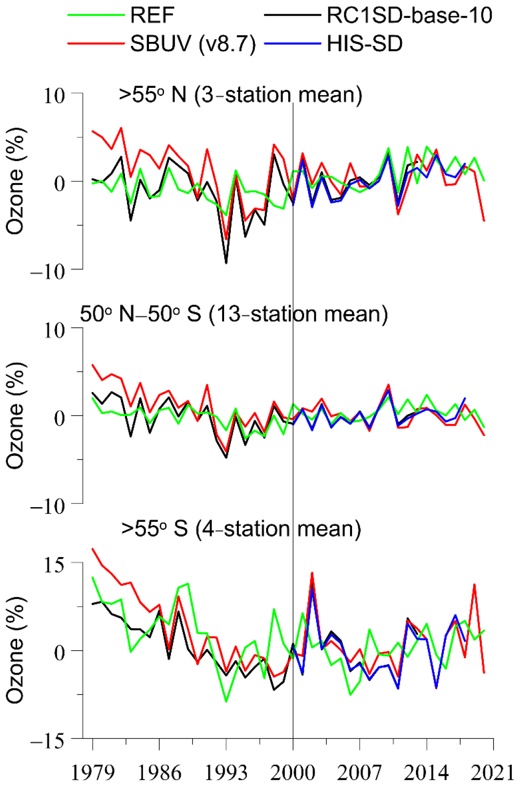
Figure A1Comparison of REF (free-running simulation; green line) with RC1SD-base-10 (SD simulation for 1979–2013; black line), HIS-SD (SD simulation for 2000–2018; blue line), and SBUV (v8.7) satellite measurements (red line) for 3 stations higher than 55∘ N (upper plot), 13 stations between 50∘ N–50∘ S (middle plot), and 4 stations higher than 55∘ S (lower plot). The vertical line has been put in the year 2000. The y axis shows yearly averaged total-ozone data (in %) calculated from de-seasonalized monthly data. The monthly data were de-seasonalized relative to the long-term monthly mean (2000–2018) and were expressed in percent. For the northern high-latitude stations, the annual average refers to the average of monthly anomalies from March to September, and for the southern high-latitude stations, it refers to the average of monthly anomalies from September to March. For the stations between 50∘ N–50∘ S we used all months to calculate the annual average.
Figure A1 shows the comparison between the simulations and SBUV data. Obviously, the RC1SD-base-10 simulation (period 1979–2013) compares much better with the SBUV data than the REF simulation. The same also holds for the HIS-SD simulation (period 2000–2018). This is expected since the SD simulation uses reanalysed meteorology, whereas the free-running simulation has its own meteorological/synoptical sequence. For comparison with the fixed-GHG simulation, we need to switch to the pair of free-running simulations. And the question is whether the evaluation (comparison with observations) also holds for the REF simulation, which is the basis for the comparison with the fixed-GHG simulation (FIX). In the case of free-running simulations, the evaluation is only possible for the trends and for the amplitude of the year-to-year variability but not for the sign of the anomaly in a given nominal year and/or month. Figure A1 shows that the free-running simulation (REF) reflects correctly the negative ozone trends of the past, seen in the observations and in the SD simulation and is therefore suitable for comparison with the fixed-GHG simulation.
Figure B1 shows the changes in the zonally averaged cloud cover based on REF (RCP 6.0) and FIX simulations and their differences (REF minus FIX) per 10∘ latitude zones from 50 to 80∘ N. For the period 1960 to 2100, the changes in cloud cover due to the evolution of GHGs (RCP 6.0) are presented in Table B1. As we move northward of 50∘ N, the same picture with increasing trends is also found for the period 2050 to 2100.

Figure B1EMAC CCM projections of zonal mean cloud cover for 10∘ latitude zones (50–60∘ N, 60–70∘ N, 70–80∘ N), based on simulations with increasing and fixed-GHG mixing ratios. (a) REF is the simulation with increasing GHGs according to RCP 6.0. FIX is the simulation with fixed-GHG emissions at 1960 levels. (b) Difference between the two model simulations, as an indicator of the impact of increasing GHGs. The y axis in (a) shows yearly averaged cloud cover data (in %) calculated from de-seasonalized monthly data. The monthly data were de-seasonalized relative to the long-term monthly mean (1990–2019) and were expressed in percent. For the northern high latitudes, the annual average refers to the average of monthly anomalies from March to September.
Table B1Changes in zonal mean cloud cover between 50 and 80∘ N due to the evolution of GHGs (RCP 6.0), for the periods 1960–2100 and 2050–2100.
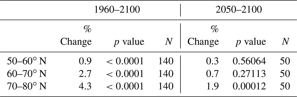
Figure C1 shows the changes in zonally averaged surface albedo based on REF (RCP 6.0) and FIX simulations and their differences (REF minus FIX) per 10∘ latitude zones between 50 and 80∘ N. Figure C2 shows the respective changes between 50 and 80∘ S. The changes in surface albedo due to the evolution of GHGs (RCP 6.0) between 50 and 80∘ N and 50 and 80∘ S are summarized in Table C1.
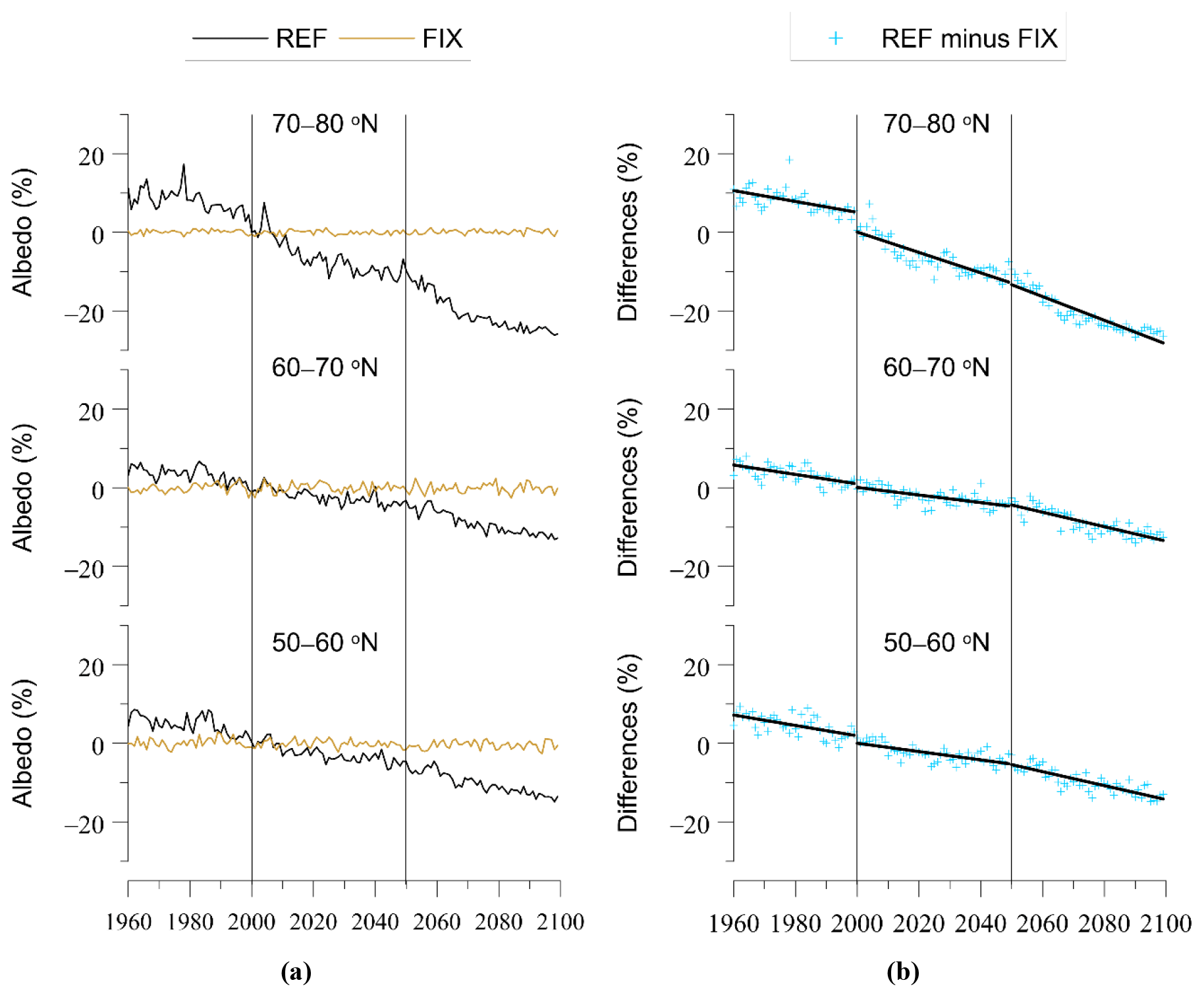
Figure C1EMAC CCM projections of zonal mean surface albedo for 10∘ latitude zones (50–60∘ N, 60–70∘ N, 70–80∘ N), based on simulations with increasing and fixed-GHG mixing ratios. (a) REF is the simulation with increasing GHGs according to RCP 6.0. FIX is the simulation with fixed-GHG emissions at 1960 levels. (b) Difference between the two model simulations, as an indicator of the impact of increasing GHGs. The y axis in (a) shows yearly averaged surface albedo data (in %) calculated from de-seasonalized monthly data. The monthly data were de-seasonalized relative to the long-term monthly mean (1990–2019) and were expressed in percent. For the northern high latitudes, the annual average refers to the average of monthly anomalies from March to September.
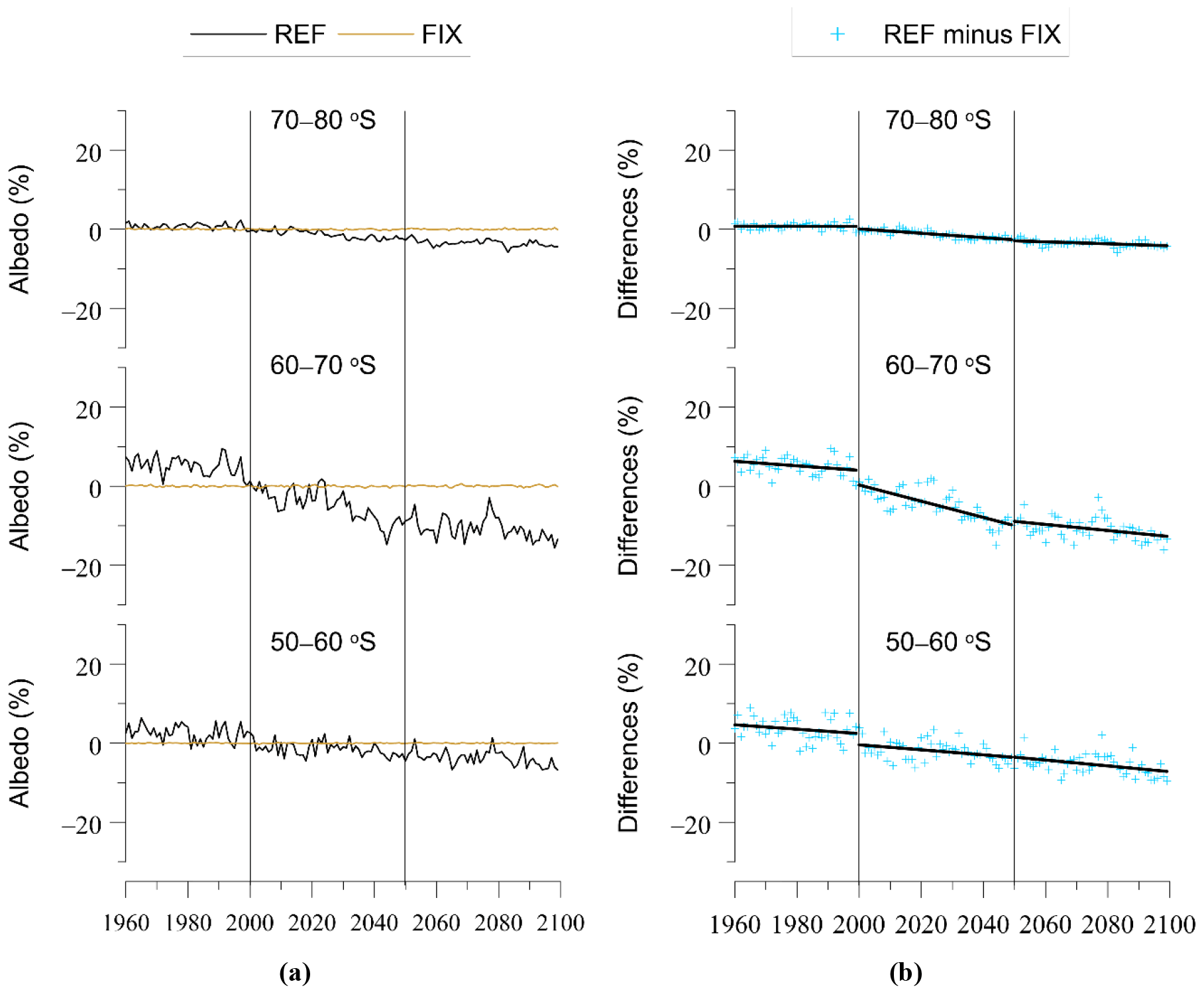
Figure C2Same as Fig. C1 but for 50–60, 60–70, and 70–80∘ S. The y axis in (a) shows yearly averaged surface albedo data (in %) calculated from de-seasonalized monthly data. The monthly data were de-seasonalized relative to the long-term monthly mean (1990–2019) and were expressed in percent. For the southern high latitudes, the annual average refers to the average of monthly anomalies from September to March.
Table C1Changes in zonal mean surface albedo due to the evolution of GHGs (RCP 6.0) between 5 and 80∘ N and 50 and 80∘ S, for the periods 1960–2100 and 2050–2100.
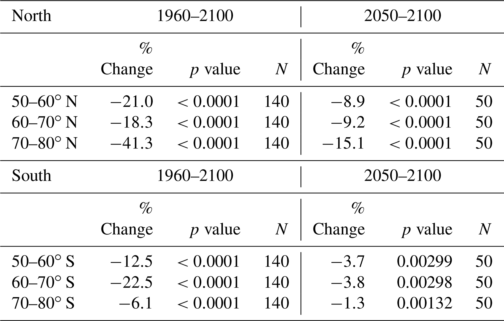
The UV irradiance data are archived in the NDACC data repository, https://www-air.larc.nasa.gov/pub/NDACC/PUBLIC/stations/ (last access: 4 September 2022; NASA, 2022a). The SBUV (v8.7) satellite ozone data are available at https://acd-ext.gsfc.nasa.gov/Data_services/merged/previous_mods.html (last access: 4 September 2022; NASA, 2022b). The MODIS Terra v6.1 satellite cloud fraction monthly mean data (MOD08_M3 v6.1) are available at https://giovanni.gsfc.nasa.gov/giovanni/#service=TmAvMp&starttime=&endtime=&data=MOD08_M3_6_1_Cloud_Fraction_Mean_Mean (last access: 4 September 2022; NASA, 2022c).
The supplement related to this article is available online at: https://doi.org/10.5194/acp-22-12827-2022-supplement.
KE and CZ conceptualized the study. AB, GB, DK, SS, BL, CB, FA, SS, HD, and KL provided ground-based UV irradiance data. KE, DK, IF, and KT analysed data. MD and PJ provided the EMAC model simulations. JK and KD processed the model simulations. The paper was originally prepared by KE and was reviewed with comments and corrections from all co-authors.
At least one of the (co-)authors is a member of the editorial board of Atmospheric chemistry and physics and at least one is a guest member of the editorial board of Atmospheric chemistry and physics for the special issue “Atmospheric ozone and related species in the early 2020s: latest results and trends (ACP/AMT inter-journal SI)”. The peer-review process was guided by an independent editor, and the authors also have no other competing interests to declare.
This article is part of the special issue “Atmospheric ozone and related species in the early 2020s: latest results and trends (ACP/AMT inter-journal SI)”. It is a result of the 2021 Quadrennial Ozone Symposium (QOS) held online on 3–9 October 2021.
Publisher’s note: Copernicus Publications remains neutral with regard to jurisdictional claims in published maps and institutional affiliations.
We acknowledge support by the project “PANhellenic infrastructure for Atmospheric Composition and climatE change” (MIS 5021516), which is implemented under the Action “Reinforcement of the Research and Innovation Infrastructure”, funded by the Operational Programme “Competitiveness, Entrepreneurship and Innovation” (NSRF 2014–2020) and co-financed by Greece and the European Union (European Regional Development Fund). The research contributes to the National Network for Climate Change and its Impact – CLIMPACT. We acknowledge the project Long-term Ozone Trends and Uncertainties in the Stratosphere (LOTUS) and the Mariolopoulos-Kanaginis Foundation for the Environmental Sciences. The EMAC simulations have been performed at the German Climate Computing Centre (DKRZ) through support from the Bundesministerium für Bildung und Forschung (BMBF). DKRZ and its scientific steering committee are gratefully acknowledged for providing the HPC and data archiving resources for the consortial project ESCiMo (Earth System Chemistry integrated Modelling). Measurements of French spectroradiometers are supported by CNES (French programme TOSCA); the Université de La Réunion and CNRS; the Région Hauts-de-France and the Ministère de l'Enseignement Supérieur et de la Recherche (CPER Climibio); and the European Fund for Regional Economic Development. Technicians at the three French and at the Finnish (Sodankylä) sites are acknowledged for the maintenance and calibration of the instruments. Kaisa Lakkala is supported by the CHAMPS project (grant no. 329225) of the Academy of Finland under the CLIHE programme. We acknowledge the SBUV science team for providing the satellite ozone profiles. NIWA UV spectrometer systems, serial numbers UV3 (Mauna Loa, HI) and UV5 (Boulder, CO), in the USA are owned and operated by NOAA/ESRL/Global Monitoring Division, Boulder CO. They are maintained, calibrated, and operated by NOAA. The final data from both of these instruments are quality controlled and produced by NIWA-Lauder, New Zealand. We thank NIWA and NOAA for the use of their data in this publication. Analyses and visualizations used in this study were produced with the Giovanni online data system, developed and maintained by the NASA GES DISC. We also acknowledge the MODIS mission scientists and associated NASA personnel for the production of the data used in this research effort. We would like to thank an anonymous reviewer for summarizing the key findings which we incorporated at the end of the conclusions.
The research work was partially funded by the Hellenic Foundation for Research and Innovation (H.F.R.I.) under the “First Call for H.F.R.I. Research Projects to support Faculty members and Researchers and the procurement of high-cost research equipment grant” (Atmospheric parameters affecting SPectral solar IRradiance and solar Energy (ASPIRE), project number 300).
This paper was edited by Stelios Kazadzis and reviewed by three anonymous referees.
Armitage, P., Berry, G., and Matthews, J. N. S.: Statistical methods in medical research, 4th Edn., Blackwell Publishing, ISBN 0-632-05257-0, 865 pp., 2001.
Bais, A. F. and Zerefos C. S.: The effect of changes in ozone on solar UV-B radiation at Reykjavik, SPIE Vol. 2049, Atmos. Ra., 263–267, 1993.
Bais, A. F., Zerefos, C. S., Meleti, C., Ziomas I. C., and Tourpali, K.: Spectral measurements of solar UVb radiation and its relations to total ozone, SO2, and clouds, J. Geophys. Res., 98, 5199–5204, 1993.
Bais, A. F., Tourpali, K., Kazantzidis, A., Akiyoshi, H., Bekki, S., Braesicke, P., Chipperfield, M. P., Dameris, M., Eyring, V., Garny, H., Iachetti, D., Jöckel, P., Kubin, A., Langematz, U., Mancini, E., Michou, M., Morgenstern, O., Nakamura, T., Newman, P. A., Pitari, G., Plummer, D. A., Rozanov, E., Shepherd, T. G., Shibata, K., Tian, W., and Yamashita, Y.: Projections of UV radiation changes in the 21st century: impact of ozone recovery and cloud effects, Atmos. Chem. Phys., 11, 7533–7545, https://doi.org/10.5194/acp-11-7533-2011, 2011.
Bais, A. F., McKenzie, R. L., Bernhard, G., Aucamp, P. J., Ilyas, M., Madronich, S., and Tourpali, K.: Ozone depletion and climate change: impacts on UV radiation, Photochem. Photobiol. Sci., 14, 19–52, https://doi.org/10.1039/c4pp90032d, 2015.
Bais, A. F., Bernhard, G., McKenzie, R. L., Aucamp, P. J., Young, P. J., Ilyas, M., Jöckel, P., and Deushi, M.: Ozone-climate interactions and effects on solar ultraviolet radiation, Photochem. Photobiol. Sci., 18, 602–640, https://doi.org/10.1039/C8PP90059K, 2019.
Bernhard, G.: Trends of solar ultraviolet irradiance at Barrow, Alaska, and the effect of measurement uncertainties on trend detection, Atmos. Chem. Phys., 11, 13029–13045, https://doi.org/10.5194/acp-11-13029-2011, 2011.
Bernhard, G. and Stierle, S.: Trends of UV Radiation in Antarctica, Atmosphere, 11, 795, https://doi.org/10.3390/atmos11080795, 2020.
Bernhard, G., Mayer, B., Seckmeyer, G., and Moise, A.: Measurements of spectral solar UV irradiance in tropical-Australia, J. Geophys. Res.-Atmos., 102, 8719–8730, https://doi.org/10.1029/97JD00072, 1997.
Bernhard, G., Booth, C. R., Ehramjian, J. C., Stone, R., and Dutton, E. G.: Ultraviolet and visible radiation at Barrow, Alaska: Climatology and influencing factors on the basis of version 2 National Science Foundation network data, J. Geophys. Res., 112, D09101, https://doi.org/10.1029/2006JD007865, 2007.
Bernhard, G., Neale, R. E., Barnes, P. W., Neale, P. J., Zepp, R. G., Wilson, S. R., Andrady, A. L., Bais, A. F., McKenzie, R. L., Aucamp, P. J., Young, P. J., Liley, J. B., Lucas, R. M., Yazar, S., Rhodes, L. E., Byrne, S. N., Hollestein, L. M., Olsen, C. M., Young, A. R., Robson, T. M., Bornman, J. F., Jansen, M. A. K., Robinson, S. A., Ballaré, C. L., Williamson, C. E., Rose, K. C., Banaszak, A. T., Häder, D.-P., Hylander, S., Wängberg, S.-Å., Austin, A. T., Hou, W.-C., Paul, N. D., Madronich, S., Sulzberger, B., Solomon, K. R., Li, H., Schkowski, T., Longstreth, J., Pandey, K. K., Heikkilä, A. M., and White, C. C.: Environmental effects of stratospheric ozone depletion, UV radiation and interactions with climate change: UNEP Environmental Effects Assessment Panel, update 2019, Photochem. Photobiol. Sci., 19, 542–584, https://doi.org/10.1039/d0pp90011g, 2020.
Bhartia, P. K., McPeters, R. D., Flynn, L. E., Taylor, S., Kramarova, N. A., Frith, S., Fisher, B., and DeLand, M.: Solar Backscatter UV (SBUV) total ozone and profile algorithm, Atmos. Meas. Tech., 6, 2533–2548, https://doi.org/10.5194/amt-6-2533-2013, 2013.
Blumthaler, M. and Ambach, W.: Indication of increasing solar ultraviolet-B radiation flux in alpine regions, Science, 248, 206–208, https://doi.org/10.1126/science.2326634, 1990.
Brühl, C. and Crutzen, P. J.: On the disproportionate role of tropospheric ozone as a filter against solar UV-B radiation, Geophys. Res. Lett., 16, 703–706, 1989.
Butchart, N.: The Brewer-Dobson circulation, Rev. Geophys., 52, 157–184, https://doi.org/10.1002/2013RG000448, 2014.
Collins, W. J., Bellouin, N., Doutriaux-Boucher, M., Gedney, N., Halloran, P., Hinton, T., Hughes, J., Jones, C. D., Joshi, M., Liddicoat, S., Martin, G., O'Connor, F., Rae, J., Senior, C., Sitch, S., Totterdell, I., Wiltshire, A., and Woodward, S.: Development and evaluation of an Earth-System model – HadGEM2, Geosci. Model Dev., 4, 1051–1075, https://doi.org/10.5194/gmd-4-1051-2011, 2011.
Dee, D. P., Uppala, S. M., Simmons, A. J., Berrisford, P., Poli, P., Kobayashi, S., Andrae, U., Balmaseda, M. A., Balsamo, G., Bauer, P., Bechtold, P., Beljaars, A. C. M., van de Berg, L., Bidlot, J., Bormann, N., Delsol, C., Dragani, R., Fuentes, M., Geer, A. J., Haimberger, L., Healy, S. B., Hersbach, H., Hólm, E. V., Isaksen, L., Kållberg, P., Köhler, M., Matricardi, M., McNally, A. P., Monge-Sanz, B. M., Morcrette, J.-J., Park, B.-K., Peubey, C., de Rosnay, P., Tavolato, C., Thépaut, J.-N., and Vitart, F.: The ERA-Interim reanalysis: configuration and performance of the data assimilation system, Q. J. Roy. Meteor. Soc., 137, 553–597, https://doi.org/10.1002/qj.828, 2011.
De Mazière, M., Thompson, A. M., Kurylo, M. J., Wild, J. D., Bernhard, G., Blumenstock, T., Braathen, G. O., Hannigan, J. W., Lambert, J.-C., Leblanc, T., McGee, T. J., Nedoluha, G., Petropavlovskikh, I., Seckmeyer, G., Simon, P. C., Steinbrecht, W., and Strahan, S. E.: The Network for the Detection of Atmospheric Composition Change (NDACC): history, status and perspectives, Atmos. Chem. Phys., 18, 4935–4964, https://doi.org/10.5194/acp-18-4935-2018, 2018.
den Outer, P. N., Slaper, H., Kaurola, J., Lindfors, A., Kazantzidis, A., Bais, A. F., Feister, U., Junk, J., Janouch, M., and Josefsson, W.: Reconstructing of erythemal ultraviolet radiation levels in Europe for the past 4 decades, J. Geophys. Res., 115, D10102, https://doi.org/10.1029/2009JD012827, 2010.
Dhomse, S. S., Kinnison, D., Chipperfield, M. P., Salawitch, R. J., Cionni, I., Hegglin, M. I., Abraham, N. L., Akiyoshi, H., Archibald, A. T., Bednarz, E. M., Bekki, S., Braesicke, P., Butchart, N., Dameris, M., Deushi, M., Frith, S., Hardiman, S. C., Hassler, B., Horowitz, L. W., Hu, R.-M., Jöckel, P., Josse, B., Kirner, O., Kremser, S., Langematz, U., Lewis, J., Marchand, M., Lin, M., Mancini, E., Marécal, V., Michou, M., Morgenstern, O., O'Connor, F. M., Oman, L., Pitari, G., Plummer, D. A., Pyle, J. A., Revell, L. E., Rozanov, E., Schofield, R., Stenke, A., Stone, K., Sudo, K., Tilmes, S., Visioni, D., Yamashita, Y., and Zeng, G.: Estimates of ozone return dates from Chemistry-Climate Model Initiative simulations, Atmos. Chem. Phys., 18, 8409–8438, https://doi.org/10.5194/acp-18-8409-2018, 2018.
Douglass, A., Fioletov, V. (Coordinating Lead Authors), Godin-Beekmann, S., Müller, R., Stolarski, R. S., Webb, A. (Lead Authors), Arola, A., Burkholder, J. B., Burrows, J. P., Chipperfield, M. P., Cordero, R., David, C., den Outer, P. N., Diaz, S. B., Flynn, L. E., Hegglin, M., Herman, J. R., Huck, P., Jánosi, I. M., Krzyscin, J. W., Liu, Y., Logan, J., Matthes, K., McKenzie, R. L., Muthama N. J., Petropavlovskikh, I., Pitts, M., Ramachandran, S., Rex, M., Salawitch, R. J., Sinnhuber, B.-M., Staehelin, J., Strahan, S., Tourpali, K., Valverde-Canossa, J., and Vigouroux, C.: Stratospheric ozone and surface ultraviolet radiation, in: Scientific assessment of ozone depletion: 2010, Global Ozone Research and Monitoring Project (Report No. 52, Chapter 2), Geneva, Switzerland: World Meteorological Organization, ISBN 978-9966-7319-6-2, 2011.
Eayrs, C., Li, X., Raphael, M. N., and Holland, D. M.: Rapid decline in Antarctic sea ice in recent years hints at future change, Nat. Geosci., 14, 460–464, https://doi.org/10.1038/s41561-021-00768-3, 2021.
Eleftheratos, K., Kazadzis, S., Zerefos, C., Tourpali, K., Meleti, C., Balis, D., Zyrichidou, I., Lakkala, K., Feister, U., Koskela, T., Heikkilä, A., and Karhu, J. M.: Ozone and spectroradiometric UV changes in the past 20 years over high latitudes, Atmos.-Ocean, 53, 117–125, https://doi.org/10.1080/07055900.2014.919897, 2015.
Eleftheratos, K., Kapsomenakis, J., Zerefos, C. S., Bais, A. F., Fountoulakis, I., Dameris, M., Jöckel, P., Haslerud, A. S., Godin-Beekmann, S., Steinbrecht, W., Petropavlovskikh, I., Brogniez, C., Leblanc, T., Liley, J. B., Querel R., and Swart, D. P. J.: Possible Effects of Greenhouse Gases to Ozone Profiles and DNA Active UV-B Irradiance at Ground Level, Atmosphere, 11, 228, https://doi.org/10.3390/atmos11030228, 2020.
Eyring, V., Lamarque, J.-F., Hess, P., Arfeuille, F., Bowman, K., Chipperfield, M., Duncan, B., Fiore, A., Gettelman, A., Giorgetta, M., Granier, C., Hegglin, M., Kinnison, D., Kunze, M., Langematz, U., Luo, B., Martin, R., Matthes, K., Newman, P., Peter, T., Robock, A., Ryerson, A., Saiz-Lopez, A., Salawitch, R., Schultz, M., Shepherd, T., Shindell, D., Stähelin, J., Tegtmeier, S., Thomason, L., Tilmes, S., Vernier, J.-P., Waugh, D., and Young, P.: Overview of IGAC/SPARC Chemistry-Climate Model Initiative (CCMI) Community Simulations in Support of Upcoming Ozone and Climate Assessments, SPARC Newsletter, 40, 48–46, 2013.
Fountoulakis, I. and Bais, A. F.: Projected changes in erythemal and vitamin D effective irradiance over northern-hemisphere high latitudes, Photochem. Photobiol. Sci., 14, 1251–1264, https://doi.org/10.1039/c5pp00093a, 2015.
Fountoulakis, I., Bais, A. F., Tourpali, K., Fragkos, K., and Misios, S.: Projected changes in solar UV radiation in the Arctic and sub-Arctic Oceans: Effects from changes in reflectivity, ice transmittance, clouds, and ozone, J. Geophys. Res.-Atmos., 119, 8073–8090, https://doi.org/10.1002/2014JD021918, 2014.
Fountoulakis, I., Zerefos, C. S., Bais, A. F., Kapsomenakis, J., Koukouli, M.-E., Ohkawara, N., Fioletov, V., De Backer, H., Lakkala, K., Karppinen, T., and Webb, A. R.: Twenty-five years of spectral UV-B measurements over Canada, Europe and Japan: Trends and effects from changes in ozone, aerosols, clouds, and surface reflectivity, Comp. Rend. Geosci., 350, 393–402, https://doi.org/10.1016/j.crte.2018.07.011, 2018.
Fountoulakis, I., Diémoz, H., Siani, A. M., Hülsen, G., and Gröbner, J.: Monitoring of solar spectral ultraviolet irradiance in Aosta, Italy, Earth Syst. Sci. Data, 12, 2787–2810, https://doi.org/10.5194/essd-12-2787-2020, 2020a.
Fountoulakis, I., Diémoz, H., Siani, A.-M., Laschewski, G., Filippa, G., Arola, A., Bais, A. F., De Backer, H., Lakkala, K., Webb, A. R., De Bock, V., Karppinen, T., Garane, K., Kapsomenakis, J., Koukouli, M.-E., and Zerefos, C. S.: Solar UV Irradiance in a Changing Climate: Trends in Europe and the Significance of Spectral Monitoring in Italy, Environments, 7, 1, https://doi.org/10.3390/environments7010001, 2020b.
Gröbner J.: Ultraviolet Radiation: Distribution and Variability, in: Encyclopedia of Sustainability Science and Technology, edited by: Meyers, R. A., Springer, New York, NY, https://doi.org/10.1007/978-1-4419-0851-3_453, 2012.
Jöckel, P., Tost, H., Pozzer, A., Kunze, M., Kirner, O., Brenninkmeijer, C. A. M., Brinkop, S., Cai, D. S., Dyroff, C., Eckstein, J., Frank, F., Garny, H., Gottschaldt, K.-D., Graf, P., Grewe, V., Kerkweg, A., Kern, B., Matthes, S., Mertens, M., Meul, S., Neumaier, M., Nützel, M., Oberländer-Hayn, S., Ruhnke, R., Runde, T., Sander, R., Scharffe, D., and Zahn, A.: Earth System Chemistry integrated Modelling (ESCiMo) with the Modular Earth Submodel System (MESSy) version 2.51, Geosci. Model Dev., 9, 1153–1200, https://doi.org/10.5194/gmd-9-1153-2016, 2016.
Jones, C. D., Hughes, J. K., Bellouin, N., Hardiman, S. C., Jones, G. S., Knight, J., Liddicoat, S., O'Connor, F. M., Andres, R. J., Bell, C., Boo, K.-O., Bozzo, A., Butchart, N., Cadule, P., Corbin, K. D., Doutriaux-Boucher, M., Friedlingstein, P., Gornall, J., Gray, L., Halloran, P. R., Hurtt, G., Ingram, W. J., Lamarque, J.-F., Law, R. M., Meinshausen, M., Osprey, S., Palin, E. J., Parsons Chini, L., Raddatz, T., Sanderson, M. G., Sellar, A. A., Schurer, A., Valdes, P., Wood, N., Woodward, S., Yoshioka, M., and Zerroukat, M.: The HadGEM2-ES implementation of CMIP5 centennial simulations, Geosci. Model Dev., 4, 543–570, https://doi.org/10.5194/gmd-4-543-2011, 2011.
IPCC (2021): Summary for Policymakers, in: Climate Change 2021: The Physical Science Basis. Contribution of Working Group I to the Sixth Assessment Report of the Intergovernmental Panel on Climate Change, edited by: Masson Delmotte, V., Zhai, P., Pirani, A., Connors, S. L., Péan, C., Berger, S., Caud, N., Chen, Y., Goldfarb, L., Gomis, M. I., Huang, M., Leitzell, K., Lonnoy, E., Matthews, J. B. R., Maycock, T. K., Waterfield, T., Yelekçi, O., Yu R., and Zhou, B., Cambridge University Press, Cambridge, United Kingdom and New York, NY, USA, 3–32 pp., https://doi.org/10.1017/9781009157896.001, 2021.
Kerr, J. B. and McElroy, C. T.: Evidence for large upward trends of ultraviolet-B radiation linked to ozone depletion, Science, 262, 1035–1034, https://doi.org/10.1126/science.262.5136.1032, 1993.
Kosmopoulos, P. G., Kazadzis, S., Schmalwieser, A. W., Raptis, P. I., Papachristopoulou, K., Fountoulakis, I., Masoom, A., Bais, A. F., Bilbao, J., Blumthaler, M., Kreuter, A., Siani, A. M., Eleftheratos, K., Topaloglou, C., Gröbner, J., Johnsen, B., Svendby, T. M., Vilaplana, J. M., Doppler, L., Webb, A. R., Khazova, M., De Backer, H., Heikkilä, A., Lakkala, K., Jaroslawski, J., Meleti, C., Diémoz, H., Hülsen, G., Klotz, B., Rimmer, J., and Kontoes, C.: Real-time UV index retrieval in Europe using Earth observation-based techniques: system description and quality assessment, Atmos. Meas. Tech., 14, 5657–5699, https://doi.org/10.5194/amt-14-5657-2021, 2021.
Krzyścin, J. W. and Baranowski, D. B.: Signs of the ozone recovery based on multi sensor reanalysis of total ozone for the period 1979–2017, Atmos. Environ., 199, 334–344, https://doi.org/10.1016/j.atmosenv.2018.11.050, 2019.
Kylling, A., Dahlback, A., and Mayer, B.: The effect of clouds and surface albedo on UV irradiances at a high latitude site, Geophys. Res. Lett., 27, 1411–1414, 2000.
Lakkala, K., Arola, A., Heikkilä, A., Kaurola, J., Koskela, T., Kyrö, E., Lindfors, A., Meinander, O., Tanskanen, A., Gröbner, J., and Hülsen, G.: Quality assurance of the Brewer spectral UV measurements in Finland, Atmos. Chem. Phys., 8, 3369–3383, https://doi.org/10.5194/acp-8-3369-2008, 2008.
Lamy, K., Portafaix, T., Josse, B., Brogniez, C., Godin-Beekmann, S., Bencherif, H., Revell, L., Akiyoshi, H., Bekki, S., Hegglin, M. I., Jöckel, P., Kirner, O., Liley, B., Marecal, V., Morgenstern, O., Stenke, A., Zeng, G., Abraham, N. L., Archibald, A. T., Butchart, N., Chipperfield, M. P., Di Genova, G., Deushi, M., Dhomse, S. S., Hu, R.-M., Kinnison, D., Kotkamp, M., McKenzie, R., Michou, M., O'Connor, F. M., Oman, L. D., Pitari, G., Plummer, D. A., Pyle, J. A., Rozanov, E., Saint-Martin, D., Sudo, K., Tanaka, T. Y., Visioni, D., and Yoshida, K.: Clear-sky ultraviolet radiation modelling using output from the Chemistry Climate Model Initiative, Atmos. Chem. Phys., 19, 10087–10110, https://doi.org/10.5194/acp-19-10087-2019, 2019.
Lucas, R. M., Yazar, S., Young, A. R., Norval, M., de Gruijl F. R., Takizawa, Y., Rhodes, L. E., Sinclair, C. A., and Neale, R. E.: Human health in relation to exposure to solar ultraviolet radiation under changing stratospheric ozone and climate, Photochem. Photobiol. Sci., 18, 641, https://doi.org/10.1039/c8pp90060d, 2019.
Madronich, S., McKenzie, R. L., Björn, L. O., and Caldwell, M. M.: Changes in biologically active ultraviolet radiation reaching the Earth's surface, J. Photochem. Photobiol. B, 46, 5–19, 1998.
Maksym, T.: Arctic and Antarctic sea ice change: contrasts, commonalities, and causes, Annu. Rev. Mar. Sci. 11, 187–213, https://doi.org/10.1146/annurev-marine-010816-060610, 2019.
McKenzie, R., Bernhard, G., Liley, B., Disterhoft, P., Rhodes, S., Bais, A., Morgenstern, O., Newman, P., Oman, L., Brogniez, C., and Simic Stana: Success of Montreal Protocol Demonstrated by Comparing High Quality UV Measurements with “World Avoided” Calculations from Two Chemistry-Climate Models, Sci. Rep., 9, 12332, https://doi.org/10.1038/s41598019-48625-z, 2019.
McKenzie, R. L., Matthews, W. A., and Johnston, P. V.: The relationship between erythemal UV and ozone, derived from spectral irradiance measurements, Geophys. Res. Lett., 18, 2269–2272, 1991.
NASA: Airborne Science Data for Atmospheric Composition, NASA [data set], https://www-air.larc.nasa.gov/pub/NDACC/PUBLIC/stations/, last access: 4 September 2022a.
NASA: SBUV Merged Ozone Data Set (MOD), 1970–2021 Profile and Total Column Ozone from the SBUV Instrument Series, NASA [data set], https://acd-ext.gsfc.nasa.gov/Data_services/merged/previous_mods.html, last access: 4 September 2022b.
NASA (Earth Data): GIOVANNI, The Bridge Between Data and Science v 4.37, NASA [data set], https://giovanni.gsfc.nasa.gov/giovanni/#service=TmAvMp&starttime=&endtime=&data=MOD08_M3_6_1_Cloud_Fraction_Mean_Mean, last access: 4 September 2022c.
Neale, R. E., Barnes, P. W., Robson, T. M., Neale, P. J., Williamson, C. E., Zepp, R. G., Wilson, S. R., Madronich, S., Andrady, A. L., Heikkilä, A. M., Bernhard, G. H., Bais, A. F., Aucamp, P. J., Banaszak, A. T., Bornman, J. F., Bruckman, L. S., Byrne, S. N., Foereid, B., Häder, D.-P., Hollestein, L. M., Hou, W.-C., Hylander, S., Jansen, M. A. K., Klekociuk, A. R., Liley, J. B., Longstreth, J., Lucas, R. M., Martinez-Abaigar, J., McNeill, K., Olsen, C. M., Pandey, K. K., Rhodes, L. E., Robinson, S. A., Rose, K. C., Schikowski, T., Solomon, K. R., Sulzberger, B., Ukpebor, J. E., Wang, Q.-W., Wängberg, S.-Å., White, C. C., Yazar, S., Young, A. R., Young, P. J., Zhu, L., and Zhu, M.: Environmental effects of stratospheric ozone depletion, UV radiation, and interactions with climate change: UNEP Environmental Effects Assessment Panel, Update 2020, Photochem. Photobiol. Sci., 20, 1–67, https://doi.org/10.1007/s43630-020-00001-x, 2021.
Nichol, S. E., Pfister, G., Bodeker, G. E., McKenzie, R. L., Wood, S. W., and Bernhard, G.: Moderation of cloud reduction of UV in the Antarctic due to high surface albedo, J. Appl. Meteorol., 42, 1174–1183, 2003.
Norris, J. R., Allen, R. J., Evan, A. T., Zelinka, M. D., O'Dell, C. W., and Klein, S. A.: Evidence for climate change in the satellite cloud record, Nature, 536, 72–75, https://doi.org/10.1038/nature18273, 2016.
Parkinson, C. L.: A 40-y record reveals gradual Antarctic sea ice increases followed by decreases at rates far exceeding the rates seen in the Arctic, P. Natl Acad. Sci. USA, 116, 14414–14423, https://doi.org/10.1073/pnas.1906556116, 2019.
Pisoft, P., Sacha, P., Polvani, L. M., Añel, J. A., de la Torre, L., Eichinger, R., Foelsche, U., Huszar, P., Jacobi, C., Karlicky, J., Kuchar, A., Miksovsky, J., Zak, M., and Rieder, H. E.: Stratospheric contraction caused by increasing greenhouse gases, Environ. Res. Lett., 16, 064038, https://doi.org/10.1088/1748-9326/abfe2b, 2021.
Riihelä, A., Bright, R. M., and Anttila, K.: Recent strengthening of snow and ice albedo feedback driven by Antarctic sea-ice loss, Nat. Geosci., 14, 832–836, https://doi.org/10.1038/s41561-021-00841-x, 2021.
Sander, R., Jöckel, P., Kirner, O., Kunert, A. T., Landgraf, J., and Pozzer, A.: The photolysis module JVAL-14, compatible with the MESSy standard, and the JVal PreProcessor (JVPP), Geosci. Model Dev., 7, 2653–2662, https://doi.org/10.5194/gmd-7-2653-2014, 2014.
Santer B. D., Wehner, M. F., Wigley, T. M. L., Sausen, R., Meehl, G. A., Taylor, K. E., Ammann., C., Arblaster, J., Washington, W. M., Boyle, J. S., and Brüggemann, W.: Contributions of Anthropogenic and Natural Forcing to Recent Tropopause Height Changes, Science, 301, 479–483, https://doi.org/10.1126/science.1084123, 2003.
Schneider, T., Kaul, C. M., and Pressel, K. G.: Possible climate transitions from breakup of stratocumulus decks under greenhouse warming, Nat. Geosci., 12, 163–167, https://doi.org/10.1038/s41561-019-0310-1, 2019.
Setlow, R. B.: The Wavelengths in Sunlight Effective in Producing Skin Cancer: A Theoretical Analysis, P. Nat. Acad. Sci. USA, 71, 3363–3366, https://doi.org/10.1073/pnas.71.9.3363, 1974.
Solomon, S., Ivy, D. J., Kinnison, J., Mills, M. J., Neely, R. R., and Schmidt, A.: Emergence of healing in the Antarctic ozone layer, Science, 353, 269–274, https://doi.org/10.1126/science.aae0061, 2016.
Stocker, T. F., Qin, D., Plattner, G. K., Tignor, M. M. B., Allen, S. K., Boschung, J., Nauels, A., Xia, Y., Bex, V., and Midgley, P. M.: Climate change 2013 the physical science basis: Working Group I contribution to the fifth assessment report of the intergovernmental panel on climate change, Cambridge University Press, Cambridge, United Kingdom and New York, NY, USA, 1535 pp., http://www.cambridge.org/9781107661820 (last access: 30 September 2022), 2013.
The HadGEM2 Development Team: G. M. Martin, Bellouin, N., Collins, W. J., Culverwell, I. D., Halloran, P. R., Hardiman, S. C., Hinton, T. J., Jones, C. D., McDonald, R. E., McLaren, A. J., O'Connor, F. M., Roberts, M. J., Rodriguez, J. M., Woodward, S., Best, M. J., Brooks, M. E., Brown, A. R., Butchart, N., Dearden, C., Derbyshire, S. H., Dharssi, I., Doutriaux-Boucher, M., Edwards, J. M., Falloon, P. D., Gedney, N., Gray, L. J., Hewitt, H. T., Hobson, M., Huddleston, M. R., Hughes, J., Ineson, S., Ingram, W. J., James, P. M., Johns, T. C., Johnson, C. E., Jones, A., Jones, C. P., Joshi, M. M., Keen, A. B., Liddicoat, S., Lock, A. P., Maidens, A. V., Manners, J. C., Milton, S. F., Rae, J. G. L., Ridley, J. K., Sellar, A., Senior, C. A., Totterdell, I. J., Verhoef, A., Vidale, P. L., and Wiltshire, A.: The HadGEM2 family of Met Office Unified Model climate configurations, Geosci. Model Dev., 4, 723–757, https://doi.org/10.5194/gmd-4-723-2011, 2011.
von der Gathen, P., Kivi, R., Wohltmann, I., Salawitch, R. J., and Rex, M.: Climate change favours large seasonal loss of Arctic ozone, Nat. Commun., 12, 3886, https://doi.org/10.1038/s41467-021-24089-6, 2021.
von Storch, H. and Zwiers, F. W.: Statistical analysis in climate research, Cambridge University Press, Cambridge, ISBN 0521450713, 484 pp., 1999.
Weatherhead, B., Tanskanen, A., Stevermer, A. (Lead Authors), Andersen, S. B., Arola, A., Austin, J., Bernhard, G., Browman, H., Fioletov, V., Grewe, V., Herman, J., Josefsson, W., Kylling, A., Kyrö, E., Lindfors, A., Shindell, D., Taalas, P., and Tarasick, D.: Ozone and ultraviolet radiation, In Arctic Climate Impact Assessment (ACIA), (Chapter 5, pp. 151–182), Cambridge University Press, https://acia.amap.no/ (last access: 4 September 2022), 2005.
Weber, M., Coldewey-Egbers, M., Fioletov, V. E., Frith, S. M., Wild, J. D., Burrows, J. P., Long, C. S., and Loyola, D.: Total ozone trends from 1979 to 2016 derived from five merged observational datasets – the emergence into ozone recovery, Atmos. Chem. Phys., 18, 2097–2117, https://doi.org/10.5194/acp-18-2097-2018, 2018.
Weihs, P., Simic, S., Laube, W., Mikielewicz, W., Rengarajan, G., and Mandl, M.: Albedo Influences on Surface UV Irradiance at the Sonnblick High-Mountain Observatory (3106-m Altitude), J. Appl. Meteorol., 38, 1599–1610, https://doi.org/10.1175/1520-0450(1999)038<1599:AIOSUI>2.0.CO;2, 1999.
Wild, M., Gilgen, H., Roesch, A., Ohmura, A., Long, C. N., Dutton, E. G., Forgan, B., Kallis, A., Russak, V., and Tsvetkov, A.: From dimming to brightening: decadal changes in solar radiation at Earth's surface, Science, 308, 847–850, https://doi.org/10.1126/science.1103215, 2005.
Zerefos, C., Meleti, C., Balis, D., Tourpali, K., and Bais, A. F.: Quasi-biennial and longer-term changes in clear sky UV-B solar irradiance, Geophys. Res. Lett., 25, 4345–4348, 1998.
Zerefos, C., Kapsomenakis, J., Eleftheratos, K., Tourpali, K., Petropavlovskikh, I., Hubert, D., Godin-Beekmann, S., Steinbrecht, W., Frith, S., Sofieva, V., and Hassler, B.: Representativeness of single lidar stations for zonally averaged ozone profiles, their trends and attribution to proxies, Atmos. Chem. Phys., 18, 6427–6440, https://doi.org/10.5194/acp-18-6427-2018, 2018.
Zerefos, C. S., Tourpali, K., Eleftheratos, K., Kazadzis, S., Meleti, C., Feister, U., Koskela, T., and Heikkilä, A.: Evidence of a possible turning point in solar UV-B over Canada, Europe and Japan, Atmos. Chem. Phys., 12, 2469–2477, https://doi.org/10.5194/acp-12-2469-2012, 2012.
Zerefos, C. S., Tourpali, K., Zanis, P., Eleftheratos, K., Repapis, C., Goodman, A., Wuebbles, D., Isaksen, I. S. A., and Luterbacher, J.: Evidence for an earlier greenhouse cooling effect in the stratosphere before 1980 over the Northern Hemisphere, Atmos. Chem. Phys., 14, 7705–7720, https://doi.org/10.5194/acp-14-7705-2014, 2014.
Zhang, R., Wang, H., Fu, Q., Rasch, P. J., and Wang, X.: Unraveling driving forces explaining significant reduction in satellite-inferred Arctic surface albedo since the 1980s, P. Natl. Acad. Sci. USA, 116, 23947–23953, https://doi.org/10.1073/pnas.1915258116, 2019.
- Abstract
- Introduction
- Data sources
- Results and discussion
- Summary and conclusions
- Appendix A: Qualitative evaluation of free-running CCM simulations against simulations with specified dynamics
- Appendix B: Model simulations of zonally averaged cloud cover between 50 and 80∘ N
- Appendix C: Model simulations of zonally averaged surface albedo between 50 and 80∘ N and 50 and 80∘ S
- Data availability
- Author contributions
- Competing interests
- Special issue statement
- Disclaimer
- Acknowledgements
- Financial support
- Review statement
- References
- Supplement