the Creative Commons Attribution 4.0 License.
the Creative Commons Attribution 4.0 License.
 | 29 Sep 2022
Peculiar COVID-19 effects in the Greater Tokyo Area revealed by spatiotemporal variabilities of tropospheric gases and light-absorbing aerosols
Alessandro Damiani
Hitoshi Irie
Dmitry A. Belikov
Shuei Kaizuka
Hossain Mohammed Syedul Hoque
Raul R. Cordero
This study investigated the spatiotemporal variabilities in nitrogen dioxide (NO2), formaldehyde (HCHO), ozone (O3), and light-absorbing aerosols within the Greater Tokyo Area, Japan, which is the most populous metropolitan area in the world. The analysis is based on total tropospheric column, partial tropospheric column (within the boundary layer), and in situ observations retrieved from multiple platforms as well as additional information obtained from reanalysis and box model simulations. This study mainly covers the 2013–2020 period, focusing on 2020 when air quality was influenced by the coronavirus 2019 (COVID-19) pandemic. Although total and partial tropospheric NO2 columns were reduced by an average of about 10 % in 2020, reductions exceeding 40 % occurred in some areas during the pandemic state of emergency. Light-absorbing aerosol levels within the boundary layer were also reduced for most of 2020, while smaller fluctuations in HCHO and O3 were observed. The significantly enhanced degree of weekly cycling of NO2, HCHO, and light-absorbing aerosol found in urban areas during 2020 suggests that, in contrast to other countries, mobility in Japan also dropped on weekends. We conclude that, despite the lack of strict mobility restrictions in Japan, widespread adherence to recommendations designed to limit the COVID-19 spread resulted in unique air quality improvements.
- Article
(12402 KB) - Full-text XML
-
Supplement
(19081 KB) - BibTeX
- EndNote


Fossil fuel combustion is the dominant source of nitrogen oxides (NOx) in the atmosphere, to which traffic is the main contributor, followed by thermal power plants. Other sources include emissions from fires, soils, and lightning. Consequently, NOx is among the main drivers of air quality degradation in urban areas, and epidemiological studies have shown that nitrogen dioxide (NO2) exposure is often associated with adverse health effects such as lung cancer, asthma, and cardiopulmonary mortality (e.g., Hamra et al., 2015; Achakulwisut et al., 2019). Therefore, NO2 is carefully monitored using both surface and satellite instruments, and it is often used as an indicator of air pollution. Moreover, NOx is a precursor to secondary aerosols and catalyzes the formation of tropospheric ozone (O3), with consequences for the climate. Due to its short lifetime on the order of a few hours, NO2 is an excellent marker for anthropogenic emissions, and satellites often show enhanced NO2 around large cities and thermal power plants (e.g., Beirle et al., 2003). Therefore, in the past, satellite NO2 observations have been exploited to evaluate the effectiveness of long-term abatement strategies, the effects of economic recessions, and the impacts of short-term emissions regulations on air quality (e.g., Russell et al., 2012; Lee et al., 2021; Vohra et al., 2022).
Along with volatile organic compounds (VOCs), NOx is a major O3 precursor. Nevertheless, in contrast to rural sites where NOx-limited conditions usually prevail, in urban locations under VOC-limited (i.e., NOx-saturated) conditions, a reduction in NOx is often associated with an increase in O3 due to reduction of the NO titration effect (Murphy et al., 2007). Indeed, in recent years, satellite observations have shown that, although NOx emissions are still rising in various developing countries (e.g., India), they have significantly decreased in the majority of the developed countries of North America, Europe, and East Asia (Russell et al., 2012; Geddes et al., 2016; Georgoulias et al., 2019), while tropospheric ozone has increased (Ziemke et al., 2019; Li et al., 2019; Lee et al., 2021). This general tendency has been confirmed in Japan (e.g., Akimoto, 2017) and, recently, in the Kanto region, where both NO2 and formaldehyde (HCHO) (as a proxy for non-methane VOCs, NMVOCs) were reduced and O3 recovered slightly during the period of 2013–2019 (Irie et al., 2021).
Due to their association with human activities, anthropogenic NOx emissions often display a weekly cycle. The term “weekend effect” refers to the difference in pollutant concentrations between weekdays and weekends (e.g., Cleveland et al., 1974). In the same manner, emissions usually decrease during holiday periods, and an equivalent “holiday effect” can be defined (e.g., Tan et al., 2009). Reduced NOx levels on rest days are often coupled with increased O3 in and around cities (Cleveland et al., 1974; Murphy et al., 2007) but not in rural areas (Sicard et al., 2020a). The weekly cycles of both NO2 and O3 have been extensively investigated in previous research using both ground-level (Cleveland et al., 1974; Sadanaga et al., 2012; Zou et al., 2019; Sicard et al., 2020a) and satellite (Beirle et al., 2003; Stavrakou et al., 2020) observations. A satellite-based analysis of the global temporal evolution of the NO2 weekly cycle showed that it has become smaller in recent years (Stavrakou et al., 2020). This trend has been explained by the current reduction in NOx emissions, confounding of anthropogenic and background NOx, and, secondarily, an increase in NO2 lifetime. On the other hand, a recent study of the O3 weekend effect revealed a significant downward trend (Sicard et al., 2020a). Overall, analysis of the response of O3 formation to emission changes supports the development of strategies to reduce precursor emissions and improve air quality.
The lockdowns caused by the coronavirus in the 2019 (COVID-19) pandemic represent an opportunity to assess the impacts of human activities on the environment and human health (Gkatzelis et al., 2021; Shakil et al., 2020; Laughner et al., 2021). Recently, many studies have shown that NO2 levels in 2020 were lower than in previous years due to reduced anthropogenic emissions associated with reduced mobility during temporary lockdowns (e.g., Bauwens et al., 2020; Venter et al., 2020; Cooper et al., 2022). Moreover, these NO2 reductions in 2020 were associated with surface O3 enhancement (Sicard et al., 2020b) and reduced O3 levels in the free troposphere (Steinbrecht et al., 2021; Miyazaki et al., 2021). Increases in surface O3 in some cities were explained by a reduction of the NO titration effect (Sicard et al., 2020b).
After the first COVID-19 cases in Wuhan, to prevent the spread of the pandemic, strong social distancing and quarantine measures were implemented in many Chinese cities as early as 24 January 2020 until about 25 February; then, measures gradually downgraded to a partial lockdown. Evident decreases in most air pollutant concentrations have been reported for China, with satellite-based NO2 reductions of about 40 % (Bauwens et al., 2020; Le et al., 2020). In February, TROPOMI NO2 and HCHO decreased to about 83 % and 11 % in Wuhan, respectively (Ghahremanloo et al., 2021). Moreover, surface observations showed a general increase in surface ozone in most regions, although ozone decreased in the subtropical south, and, besides the reduced emissions, meteorological changes were found to be important contributors (Sicard et al., 2020b; Le et al., 2020; Liu et al., 2021). In Korea, the most significant changes occurred in March, with a reduction of about 20 % in NO2 and 45 % in PM2.5 nationwide, while surface ozone, in contrast with China, was slightly decreased (Ju et al., 2021).
Overall, data from various sources suggest a decline in worldwide mobility in 2020 (Nouvellet et al., 2021). Figure 1 shows the change in mobility (number of people transiting public stations, derived from Google) compared to the pre-COVID period for some large metropolitan areas around the world deeply affected by the pandemic (further details in Sect. 2.1.7). The larger reductions (with peaks over 90 %) generally coincided with lockdowns, which occurred at slightly different times in different countries. Outside lockdowns, mobility remained markedly decreased throughout 2020.

Figure 1Google mobility data for the place category of transit stations in 2020 (from 15 February to 31 December) compared to the pre-COVID period for selected large metropolitan areas around the world strongly affected by the pandemic. For Japan and Italy, values were averaged (thick line) over nine (Tokyo, Kanagawa, Saitama, Chiba, Kyoto, Nara, Osaka, Fukuoka, Nagasaki) and four (Milan, Rome, Naples, and Turin) cities or prefectures (thin lines), respectively: (a) time series; (b) weekly changes. Holidays were removed. The baseline in both (a) and (b) is the median value for the corresponding day of the week during the 5-week period of 3 January–6 February 2020.
In Japan, the change in mobility was smaller and more gradual compared to other countries due to the avoidance of strict legal restrictions. However, on 3 February, Japan began addressing the issue of the Diamond Princess cruise ship quarantine, and on 3 March, primary and secondary schools were closed and replaced with remote learning (Table 1). Then, an official state of emergency, when the most stringent restrictions were in effect, was declared from 7 April to 25 May. Thereafter, the situation never returned to normal, as new periods of reduced mobility coincided with the second wave of coronavirus infections, which peaked in July–September, and the third wave starting in December.

Generally, the mean reduction in mobility was similar among all weekdays and slightly smaller during the weekend in most of the examined countries (Fig. 1b). In contrast to this worldwide trend, Japan showed the largest mobility drop during the weekend, with decreases about 10 % larger than on weekdays. Although limited to the state of emergency period and the Tokyo area, this behavior has been observed from other data sources (e.g., Fig. 2 in Sugawara et al., 2021) and appears to be a robust feature representing common Japanese habits modified by the spread of the pandemic.
Due to this anomalous change in mobility, we suggest that the (relative) NO2 weekend effect in 2020, primarily driven by traffic, may show peculiar characteristics in Japan. Potentially, this effect could be larger than usual, despite reduced NOx emissions tending to reduce the anthropogenic weekly signature (Stavrakou et al., 2020). This unique situation provides the opportunity to examine the changes in air quality that occurred in 2020 in Japan and compare them with previous years.
As detailed above, many previous studies examined COVID-related changes in air quality on a global to local scale. Nevertheless, due to somewhat soft countermeasures to limit the spread of the pandemic adopted in Japan with consequent more limited changes in mobility compared with other countries, relatively fewer studies focused on this area (e.g., Itahashi et al., 2022). In some cases, changes in relevant air quality parameters observed by ground-based or satellite instruments in the Tokyo center during the emergency period have been examined on a local scale (Sugawara et al., 2021) or related to other cities and/or countries on a global scale (e.g., Cooper et al., 2022) within studies aimed at comparing such variabilities with mobility changes. Nevertheless, as we will see, such changes hide sizable spatiotemporal variability and widespread adherence to recommendations designed to limit the spread of the pandemic, which caused modification of common habits. Those resulted in a unique air quality signature not limited to the emergency period, which should be examined on a regional scale.
We focused our study on the Greater Tokyo Area (GTA) in the Kanto region, which is the largest area of flat land in Japan, extending inland from the Pacific coast (Fig. 2). It is the most populous metropolitan area in the world and the most important economic hub of East Asia, and local emissions dominate it. Most of this large urban area is expected to be under VOC-limited conditions (Akimoto, 2017; Irie et al., 2021). Nevertheless, western Japan and, to a lesser extent, this region are usually affected by transboundary air pollution from the continent (Itahashi et al., 2022). Due to the strict mobility restrictions implemented in China, this additional contribution is expected to be reduced in early 2020 (Itahashi et al., 2022). This makes the analysis of the COVID-related effects even more complex and points to the necessity of a regional study focusing on spatiotemporal variability.
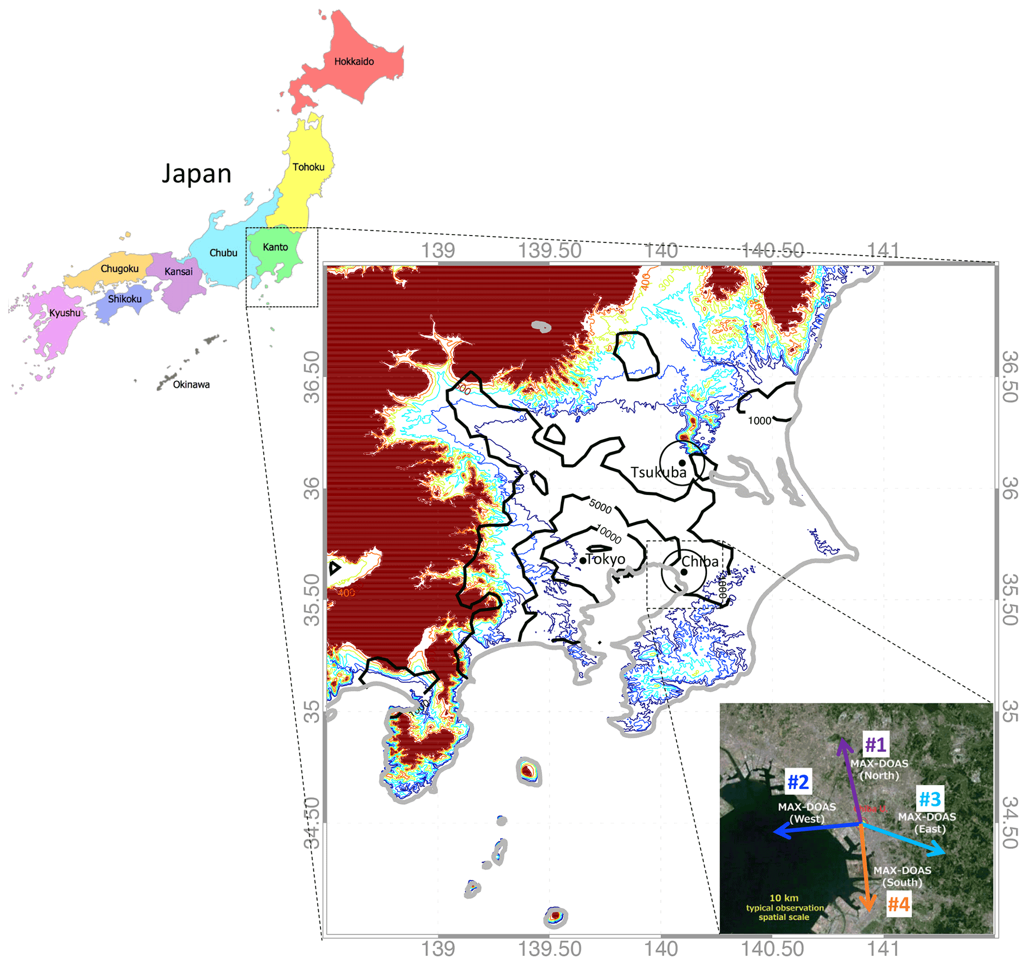
Figure 2Main panel: terrain map (meters above sea level, colored isolines; elevations >0.5 km shaded dark red) from the General Bathymetric Chart of the Oceans (GEBCO) 2021 and population density (black isolines, people per square kilometer) from the Gridded Population of the World Version 4 (GPWv4). Circles highlight the average area sampled by the MAX-DOAS system (four azimuthal directions for Chiba, one direction for Tsukuba). The top inset shows the location of the investigated Kanto region in Japan, and the bottom inset (© Google Maps 2019) shows the azimuthal pointing directions of the four MAX-DOAS systems deployed at Chiba University.
In this study, we apply an integrated approach that exploits various independent datasets retrieved from multiple platforms, including observations of NO2, O3, and HCHO (as a proxy for non-methane VOCs, NMVOCs; Sillman, 1995) from two sites equipped with multi-axis differential optical absorption spectroscopy (MAX-DOAS) systems located in urban and suburban areas. Further, anthropogenic light-absorbing aerosol data are presented. In contrast to most previous studies, which have focused on in situ and satellite-based data, observations representative of the boundary layer (<1 km) provide our reference data to link surface and satellite column observations.
2.1 Datasets
2.1.1 MAX-DOAS
We used MAX-DOAS observations from the Chiba University (in 2013–2020) and Tsukuba (in 2015–2020) sites, which are located in urban and semi-urban environments within the Kanto region (Fig. 2). The MAX-DOAS technique is based on the well-established DOAS technique (Platt and Stutz, 2008), which utilizes differential absorption structures of trace gases in ultraviolet (UV) and visible (Vis) wavelength regions to derive aerosol and trace gas information (Hönninger et al., 2004). Our MAX-DOAS system is equipped with a UV–Vis spectrometer located indoors, while an outdoor telescope unit collects scattered sunlight at reference and off-axis elevation angles. A set of scattered sunlight spectra was measured in a 15 min interval. High-resolution spectra were recorded from 310 to 515 nm using the Maya2000Pro spectrometer (Ocean Insight, Inc., Orlando, FL, USA) with a slit of 25 µm and a full width at half-maximum of approximately 0.3–0.4 nm, embedded in a temperature-controlled box. Wavelength calibration was performed daily using a high-resolution solar spectrum to account for potential long-term degradation of the spectrometer. Retrieval was conducted based on DOAS and optimal estimation methods using the Japanese MAX-DOAS profile retrieval algorithm version 2 (JM2) (Irie et al., 2011, 2015) for the following purposes: DOAS fitting, retrieval of the aerosol profile, and retrieval of trace gases. In this study, partial vertical columns of O3, NO2, and HCHO concentrations below 1 km were used. Notably, due to the contribution of upper troposphere–lower stratosphere (UTLS) O3 to differential slant column densities, only data collected at a solar zenith angle (SZA) below 50∘ can be used for O3 retrieval (Irie et al., 2011, 2021). Therefore, the ozone dataset employed here was limited to the period of March–October. For cloud screening, measurements with retrieved aerosol optical depth (AOD) greater than 3 and relative humidity over water greater than 90 % were excluded (Takashima et al., 2009). The uncertainty in the retrieved profiles was further reduced by averaging the data from four collocated MAX-DOAS instruments pointing in four different directions at the Chiba site (see inset in Fig. 2). This procedure is expected to better account for the potential spatial heterogeneity of tropospheric gases. By contrast, observations from a single MAX-DOAS system were used for the Tsukuba site. The MAX-DOAS horizontal viewing distance depends on atmospheric conditions (i.e., aerosol load) and can be up to 24 km in the lowest 1 km vertical layer. Therefore, the MAX-DOAS partial column observations at Chiba are representative of the boundary layer across a region larger than (or comparable to) a usual satellite pixel but sampled at higher accuracy. Within this framework, it is worth highlighting that our MAX-DOAS observations contributed to recent efforts of the scientific community to validate TROPOMI NO2 and HCHO datasets at a global scale (Verhoelst et al., 2021; De Smedt et al., 2021).
2.1.2 TROPOMI
The Tropospheric Monitoring Instrument (TROPOMI) onboard the European Union Copernicus Sentinel 5 Precursor (S5P) satellite has a Sun-synchronous orbit with a daily Equator crossing time of approximately 13:30 local solar time and daily global coverage (van Geffen et al., 2022). The pixel size of TROPOMI was initially 3.5 × 7 km2 and was reduced to 3.5 × 5.6 km2 (August 2019), while the swath width is 2600 km. The imaging spectrometer of this instrument measures radiation in the UV, Vis, near-infrared, and shortwave infrared spectral regions (De Smedt et al., 2021; Veefkind et al., 2012). Operational level 2 (L2) products retrieved from TROPOMI observations include vertical columns of O3, NO2, HCHO, carbon monoxide (CO), sulfur dioxide (SO2), and methane (CH4). In the following analysis, we used the official TROPOMI NO2 and HCHO products from the Tropospheric Emission Monitoring Internet Service and the Copernicus Open Access Hub, respectively, recorded between January 2019 and December 2020. As in previous studies (e.g., Barré et al., 2021), the datasets were binned and averaged over a regular grid of 0.1 × 0.1∘ to perform various statistical analyses at each location (i.e., grid box).
The TM5-MP-DOMINO NO2 data used in this study are based on the DOMINO retrieval (van Geffen et al., 2022), which was previously used for Ozone Monitoring Instrument (OMI) data, and exploit the 405–465 nm spectral range to render tropospheric vertical column density with precision of 30 %–40 %. The profile shape of the TM5-MP model is used for computation of the air mass factor (AMF) without accounting for aerosols. Screening of TROPOMI NO2 data involved retaining data with a quality flag (QF) value higher than 0.5 and a cloud fraction (CF) lower than 0.2. The TM5-MP-DOMINO NO2 dataset combines versions 1.2.x and 1.3.x. Version 1.3.x was introduced on 6 February 2019, so, essentially, it covers the entire period examined here. Minor differences exist between versions 1.2.x and 1.3.x, and, according to all past studies, we combined them (van Geffen et al., 2022). These differences were caused by improvements in the FRESCO-S algorithm devoted to retrieving cloud information. Indeed, since version 1.3.x, to avoid nonphysical cloud fraction and pressure values, when the top-of-atmosphere reflectance is lower than expected, the surface albedo is reduced to match the top-of-atmosphere reflectance (van Geffen et al., 2022). A further change in FRESCO is the treatment of very high cloud fractions (van Geffen et al., 2022). Nevertheless, we excluded observations retrieved under these conditions.
A retrieval algorithm developed for the OMI QA4ECV products is used to retrieve TROPOMI L2 HCHO vertical column densities. HCHO slant column densities are retrieved in the 328.5–359 nm fitting window. The HCHO vertical columns are calculated from the retrieved slant column densities and AMF, which is based on TM5-MP. TROPOMI L2 cloud products provide cloud information for AMF calculations. A more explicit explanation of the TROPOMI HCHO retrievals and their validation is provided in the works of De Smedt et al. (2018, 2021). Data filtering was performed as detailed in the product read-me file (http://www.tropomi.eu/sites/default/files/files/publicSentinel-5P-Formaldehyde-Readme.pdf, last access: 23 September 2022). The current TROPOMI HCHO product is based on version 2.1.3 after 13 July 2020 and version 1.1.x for the period before (De Smedt et al., 2021). Version 2.1.3 includes various improvements compared to the previous version 1.1.x, such as a new surface albedo retrieval algorithm, the adoption of new OCRA cloud-free maps, and the correction of some QF values over snow–ice regions (the latter did not affect the investigated area). More information can be found in the product read-me file and recent validation activities (De Smedt et al., 2021).
2.1.3 OMI
OMI is on board the National Aeronautics and Space Administration (NASA) Aura satellite, which has a Sun-synchronous polar orbit. OMI passes the Equator around 13:40 LT (local time), and the size of its pixels is 13 km × 24 km at nadir.
We used OMI NO2 Level-2 data (over Chiba University and Tsukuba sites) and the recently updated Level-3 daily global gridded (0.25 × 0.25∘) OMNO2d data V4. The algorithm includes improved surface and cloud treatments (Lamsal et al., 2021). In the following analysis, we exploit observations recorded in 2005–2020 and screen out NO2 data associated with a cloud fraction larger than 0.3. OMI and TROPOMI NO2 datasets are based on slightly different retrieval algorithms, including cloud algorithms to estimate cloud fraction. Moreover, the size of the field of view of OMI is larger than that of TROPOMI, and OMI is affected by the row anomaly problem (http://omi.fmi.fi/anomaly.html, last access: 23 September 2022), which further reduces the number of available observations. Here, the slightly larger cloud fraction threshold for OMI than that of TROPOMI tends to counteract the smaller number of available OMI observations (by adding a further 10 % of data; more information on the variation of OMI NO2 as a result of modifying screening criteria can be found in Compernolle et al., 2020). Since OMI O3 only has some low sensitivity to the boundary layer while TROPOMI O3 is currently limited to tropical latitudes, we did not use satellite-based O3 datasets in this study.
2.1.4 Surface in situ and additional ground observations
In Japan, continuous monitoring of NOx and other compounds through a capillary surface network is performed by the Atmospheric Environmental Regional Observation System (AEROS). Historical time series data are accessible to the public via the geographic information system (GIS) of the National Institute for Environmental Studies (NIES) (http://www.nies.go.jp/igreen/index.html, last access: 10 January 2022). As the most recent years are unavailable from the NIES catalog, we limited our analysis to NO2 observations in 2015–2018. We used a total of 266 stations, including general atmosphere measurement stations and automobile exhaust gas measurement stations in Tokyo, Chiba, and Ibaraki prefectures. The measurement principles of O3, NOx, and non-methane hydrocarbons are based on UV absorption, NO–O3 chemiluminescence, and flame ionization detection, respectively.
In addition to the NIES dataset, we used observations of black carbon (BC) concentrations recorded by the continuous soot-monitoring system (COSMOS) (Kondo et al., 2009; Damiani et al., 2021) deployed at Chiba University site in November 2019. Our analysis focused on observations recorded in 2020.
Finally, we combined optical property information retrieved by a sky radiometer with MAX-DOAS data to estimate light-absorbing aerosols within the boundary layer (Damiani et al., 2021), as described in Sect. 2.2.
2.1.5 CLASS model
Simulations with a box model accounting for boundary layer dynamics and chemistry were performed using the Chemistry Land-surface Atmosphere Soil Slab (CLASS) model (van Stratum et al., 2012; Vilà-Guerau de Arellano et al., 2015). In these simulations, we used fixed dynamic (i.e., the usual boundary layer height recorded by the collocated lidar instrument) and chemistry conditions (as in van Stratum et al., 2012), along with the concentrations of NO2 and HCHO recorded by the MAX-DOAS system within the boundary layer (at altitudes lower than 1 km) as initial conditions. The model solves the diurnal evolution of dynamical and chemical species over time in a well-mixed convective planetary boundary layer (PBL) (Vilà-Guerau de Arellano et al., 2015). Since these variables are assumed to be constant with height, the model output approximates MAX-DOAS observations in the PBL. Chemistry is represented by an Ox–NOx–VOC–HOx photochemistry scheme based on 28 reactions that control O3 formation. Although this simplified scheme omits other important organic species and aerosols, CLASS has been shown to reproduce the observed diurnal variability and mixing ratios of the main reactants present in polluted environments (Zara et al., 2021, and references therein).
2.1.6 Copernicus Atmosphere Monitoring Service (CAMS) global reanalysis
CAMS global reanalysis (EAC4) is the latest global reanalysis dataset of atmospheric composition produced by the European Centre for Medium-Range Weather Forecasts (ECMWF), including aerosols, chemical species, and greenhouse gases (Inness et al., 2019). Atmospheric data are interpolated to 25 pressure levels (top level, 0.1 hPa) at a spatial resolution of 0.7 × 0.7∘. Notably, both OMI (overpass around 13:40 LT) and GOME-2 (overpass around 10:00 LT) NO2 data are assimilated in CAMS, but anomalous emissions that occurred in 2020 are not included; i.e., the simulations are based on a business-as-usual emissions scenario. Instead, CAMS uses MACCity anthropogenic emissions and the CO emissions upgrade described by Stein et al. (2014). Monthly mean VOC emissions were calculated using the MEGAN model.
2.1.7 Additional datasets
Ozonesondes were launched from the Tateno Aerological Observatory (Tsukuba, Japan) by the Japan Meteorological Agency (JMA), usually at 15:00 (i.e., around the anticipated time indicating maximum ozone). The KC ozonesonde used until November 2009 was replaced with an electrochemical concentration cell (ECC) ozonesonde in December 2009. In some of the following analyses, to fill the gap of the absence of MAX-DOAS O3 observations in winter (see Sect. 2.1.1), we used data recorded in the period of 2013–2020 for consistency with the MAX-DOAS time series.
MERRA-2 is NASA's latest reanalysis and includes online aerosol fields that interact with model radiation fields (Buchard et al., 2017; Randles et al., 2017). This product is based on coupling of the Goddard Earth Observing System Version 5 Earth system model with the Goddard Chemistry Aerosol Radiation and Transport aerosol model. The resolution is 0.625 × 0.5∘ with 72 vertical layers from the surface to approximately 80 km. In the following analysis, we employ data for wind speed, temperature, and PBL height (PBLH).
Following previous studies (e.g., Guevara et al., 2021), we used Google mobility data as a proxy for traffic counts as they are easily accessible for the majority of the countries and allowed us to compare the changes that occurred in different regions. Google mobility data show changes to visits to various places worldwide (https://www.google.com/covid19/mobility/, last access: 10 January 2022). Visits on each day are compared to baseline values for that day of the week. The baseline is the median value for the corresponding day of the week during the 5-week period of 3 January–6 February 2020. The following place categories are available: grocery and pharmacy, parks, transit stations, retail and recreation, residential, and workplaces. Here, we focused on changes in the transit stations category (Fig. 1) in certain large metropolitan areas of the world deeply affected by the pandemic. Google transit data have been previously used to estimate the emission reduction for the road transport sector (Guevara et al., 2021). They assume that mobility trends in public transport hubs can be taken as a proxy for trends in road traffic emissions. This assumption is likely more appropriate for lighter vehicles than for heavier vehicles (Brancher, 2021).
2.2 Methods
Except where otherwise noted, we focus on ground-based daily observations recorded between 09:00 and 15:00 LT. Weekly changes in NO2, HCHO, O3, and light-absorbing aerosols are reported as differences with respect to the average value on weekdays. As the strongest reduction of anthropogenic emissions occurs on Sunday in the investigated region, we refer to weekly changes as the difference between the Sunday value and the average of the weekdays. The holiday effect was estimated to be the difference between the average concentration of a given compound during the given holiday period and that in the two 10 d periods immediately before and after the holiday.
Light-absorbing aerosols within the boundary layer were estimated by combining sky radiometer and MAX-DOAS optical property data at UV wavelengths (Damiani et al., 2021). Then, in the following analysis, we examine the fine-mode absorbing AOD within the partial column below 1 km (i.e., fAAOD, 0–1 km), which was computed by combining the columnar fine-mode fraction (FMF) and single-scattering albedo (SSA) parameters retrieved from the sky radiometer with the mean partial column AOD estimated from MAX-DOAS measurements. As mineral dust can be strongly absorbing in the UV spectral range, we further removed days with Ångström exponent (AE) < 1.
Under days characterized by stagnant low wind speed conditions, NO2 accumulates around source locations. In contrast, under days with high wind speed conditions, NO2 is dispersed. Tokyo is located in a polluted background with various significant NOx sources surrounding it within about a 100 km radius. Therefore, due to the influence of surrounding sources, the outflow plume of NO2 from Tokyo is not evident in the TROPOMI NO2 maps. However, the spatial pattern of the difference between these two NO2 composites, built based on wind speed data, reveals outflow patterns more clearly (see also Liu et al., 2016). We applied this method limitedly to Fig. 5c. To select the threshold values to identify high and low wind speed days for each pixel, we used MERRA-2 wind fields. According to previous studies (e.g., Fioletov et al., 2022), we used a PBL-averaged wind. Still, the results are not sensitive to the wind altitude because the wind is relatively constant within the boundary layer. Composite differences between high and low wind speed days in TROPOMI NO2 were computed based on MERRA-2 wind fields averaged around the overpass time (12:00–15:00). The median wind speed of each pixel was assumed to be the threshold between the high and low wind values. We first regridded the MERRA-2 data to the resolution of TROPOMI; then, for each grid cell, we computed NO2 as the difference between the composite values of days with high and low wind speed.
3.1 Trends and seasonal changes
The spatial distribution of the TROPOMI NO2 and HCHO column data in the Kanto region is shown in Fig. 3 for 2019 and 2020 on an annual basis (top panels) and during the state of emergency (bottom panels). The bulk of NO2 is around Tokyo, which is the most densely populated area (Fig. 2), including along the main transportation routes, and extends toward the south, where various large power plants and industrial activities are located (left column in Fig. 3). Overall, on an annual basis, column NO2 over the GTA was reduced by about 10 % in 2020 compared to 2019 (Fig. 3m), with larger absolute reductions around Haneda and Narita international airports, while smaller changes occurred in areas characterized by the presence of multiple power plants (south of Chiba). On the other hand, during the state of emergency, TROPOMI shows the largest NO2 reduction (20 %–40 %) in the southern Tokyo area, while limited reductions (about 10 %) occurred around Chiba and Tsukuba (Fig. 3o). The area affected by the most significant NO2 reduction coincides with the region characterized by the larger decrease in traffic counts (Takane et al., 2022). Assuming that traffic currently contributes about 40 % of Japanese domestic NOx emissions (Kurokawa and Ohara, 2020), a drop in mobility by about 50 % in April–May (Fig. 1) is consistent with the TROPOMI-based estimate of NO2 changes related to COVID.
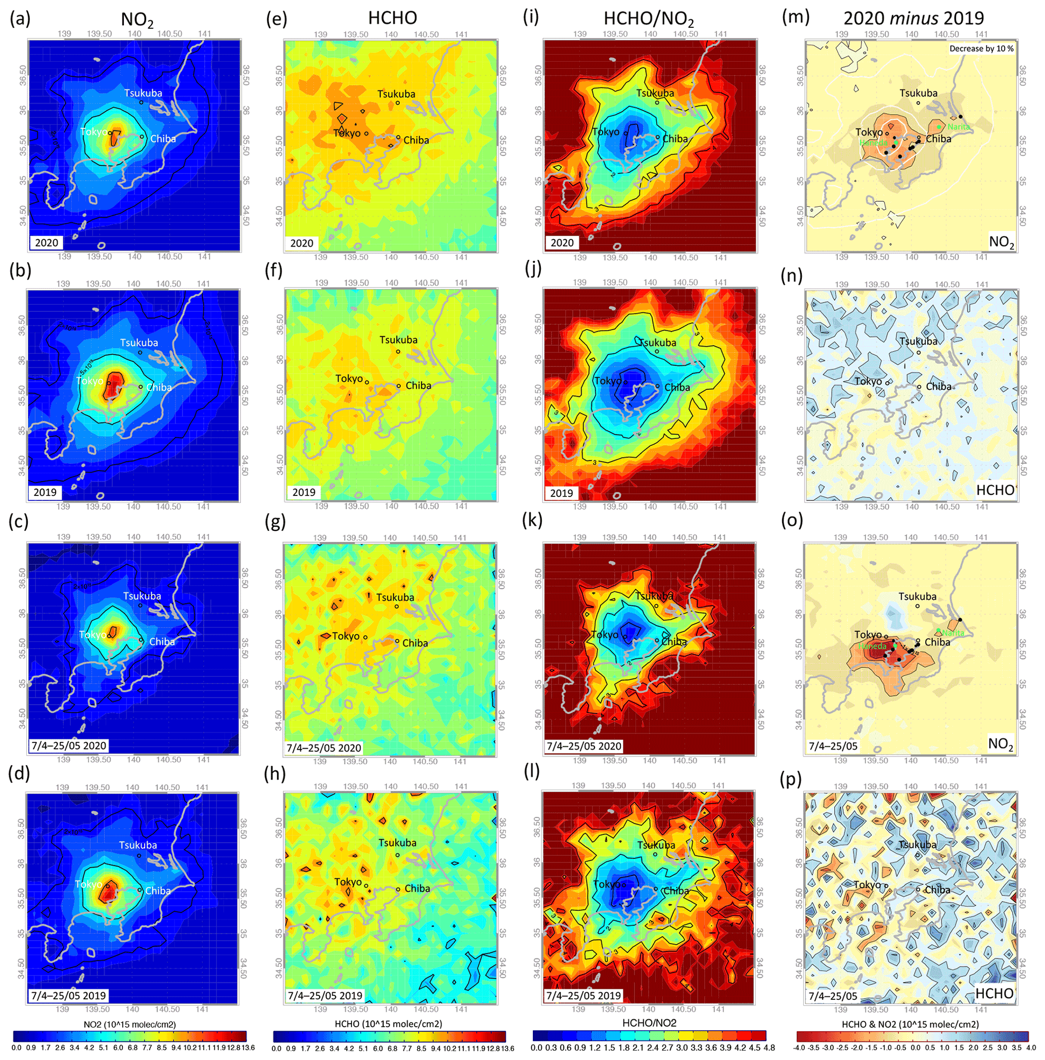
Figure 3Top two rows of panels: spatial distribution of TROPOMI NO2 (a, b), HCHO (e, f), and (i, j) in 2020 and 2019, as well as the 2020–2019 differences in NO2 (m) and HCHO (n). Bottom two rows of panels: the spatial distribution of TROPOMI observations is as described above but limited to 7 April–25 May (i.e., the state of emergency).
Aside from anthropogenic emissions, meteorological conditions contribute to determining the interannual variability of NO2. Annual differences between 2020 and 2019 in major meteorological parameters such as wind speed, surface temperature, and PBLH, which are expected to influence the NO2 distribution, were quite limited (Fig. S1a–c in the Supplement). In contrast, during the state of emergency, the wind speed in 2020 was slightly higher than that of 2019 and potentially contributed to further reducing the NO2 levels (Fig. S1d).
Based on satellite observations and model simulations, Cooper et al. (2022) estimated a significant overall decrease in surface NO2 over more than 200 cities around the world in April 2020 compared with 2019. Among others, they reported NO2 changes for various Japanese cities. Within the Kanto region, they showed reductions peaking at Yokohama (−69 %), more minor changes at Saitama (−32 %), and values roughly in between at Tokyo (−54 %). Despite the inverse correlation between the lockdown stringency index and NO2, they found that changes in Japan were comparable to or slightly lower than those for the European cities where lockdown restrictions were much more stringent. In agreement with our findings (Figs. S1d and S3), they showed that changes in Japan could have been favored by meteorology and long NO2 trends. Although the period examined by Cooper et al. (2022) only partially coincides with the Japanese state of emergency, Fig. 3o shows comparable reductions. Moreover, Fig. 3o reveals the complex pattern of these variations, characterized by an evident north–south gradient with the most significant (negative) changes in southern Tokyo, further evolving toward zero changes in the Saitama prefecture. This highlights the necessity of coupling detailed analysis at a regional scale with a large-scale study when examining COVID-related impacts, particularly when focusing on areas dominated by several close megacities.
Despite the high spatial heterogeneity of HCHO concentrations due to its short lifetime, the spatial distribution of the TROPOMI HCHO column was estimated (panels e–h in Fig. 3). While NO2 variability is dominated by anthropogenic activities, HCHO arises from both anthropogenic and natural sources. The principal source of HCHO is the oxidation of methane, which provides a global ambient background (e.g., Surl et al., 2018). Then, over continental atmospheres, the main anthropogenic sources are vehicle exhaust emissions and industrial emissions, while the main natural sources are plants and biomass burning (Surl et al., 2018; Sun et al., 2021; Ghahremanloo et al., 2021). Although the general increasing gradient from the ocean toward the continent resembles the pattern of NO2, the HCHO distribution is not well defined and does not align with the urbanized region. The somewhat higher HCHO concentration in 2020 (Fig. 3n), despite lower anthropogenic emissions, may be driven by small differences in temperature between the 2 years (Fig. S1b). However, the change in meteorological conditions and the application of cloud screening cause the amount of data collected under clear-sky conditions to be slightly different each year. Then, the distribution along the year of the data can also be different. For example, due to the rise in the summertime HCHO concentration, if frequent clouds caused few TROPOMI observations collected in the summer of a given year, the mean annual concentration of such a year could be smaller than the mean of the other year characterized by more summer HCHO observations. This confounding factor complicated the interpretation of HCHO changes. Then, despite the lower temperature that occurred during the state of emergency (Fig. S1e), TROPOMI did not show evident differences in the HCHO pattern between the 2 years (Fig. 3p).
A summer maximum characterizes the observed seasonal cycle of the HCHO columns shown in Fig. 4g. This indicates that biogenic emissions dominate HCHO even within our urban region. Pieces of evidence in TROPOMI HCHO reductions as a consequence of the COVID-related mobility restrictions have been reported only for China (Ghahremanloo et al., 2021), while meteorology likely drove most of the HCHO variations in India (Levelt et al., 2022). However, even in Wuhan, while the reduction in NO2 reached about 83 %, the decrease in HCHO was only 11 %. The recent study by Sun et al. (2021) showed that comparable HCHO reductions (i.e., 11 %) were found in the Northern China Plain for locations with predominant declines in NO2 columns and elevated anthropogenic NMVOC emissions. However, reductions were favored by meteorological conditions. Then, simulations showed that most of the HCHO decrease resulted from the reduced anthropogenic NOx emissions. Still, an additional reduction in anthropogenic NMVOC emissions of about 15 % would be necessary to match the observations (Sun et al., 2021). Since mobility restrictions in Japan were less severe and more gradual than those established in China, we expect such minor HCHO variations to be hardly identifiable by using satellite observations.
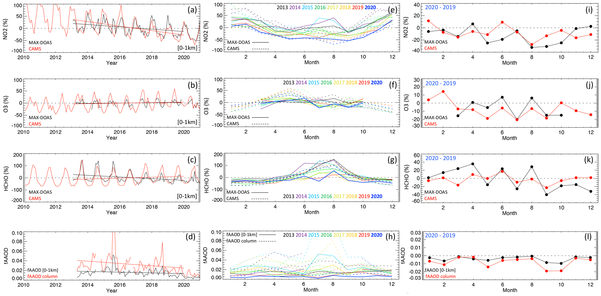
Figure 4(a–d) Monthly time series of NO2 (a), O3 (b), and HCHO (c) partial tropospheric column (<1 km) as recorded by the MAX-DOAS system and estimated by CAMS at Chiba University. (e–h) Seasonal monthly changes in MAX-DOAS observations and CAMS estimates of NO2 (e), O3 (f), and HCHO (g). (i–l) Differences (2020 minus 2019) in MAX-DOAS observations and CAMS estimates for NO2 (i), O3 (j), and HCHO (k). Results are shown as percentage changes with respect to the 2013–2019 average (left and central panels) and 2019 (right panels). (d, h, l) Changes as described above but for fine-mode light-absorbing aerosols, i.e., fAAOD and fAAOD (0–1 km).
The HCHO-to-NO2 concentration ratio is an indicator of near-surface O3 sensitivity (e.g., Martin et al., 2004). Traditionally, the ozone production regime is considered to be VOC-limited when this ratio is lower than 1 and NOx-limited when it is higher than 2, while ozone is expected to be in the transition regime when the values are in the range 1–2 (Duncan et al., 2010; Ryan et al., 2020). Although several studies used this ratio to infer O3 sensitivity to NOx and VOCs by using observations from satellite and ground-based instruments (Duncan et al., 2010; Jin et al., 2017; Schroeder et al., 2017; Irie et al., 2021), some limitations still exist. Assuming the transition region lies within the range 1–2 (Duncan et al., 2010) could not be valid at global levels, and it could be necessary to compute it depending on the region (Schroeder et al., 2017). Moreover, the ratio has an altitude dependence (e.g., Jin et al., 2017; Schroeder et al., 2017). While seasonal variations and trends in the columnar ratio (i.e., based on satellite observations) generally match the ratio computed with in situ observations, magnitudes are often different due to different vertical distributions of HCHO and NO2 (Ryan et al., 2020). Therefore, although O3 sensitivity derived from satellite column data can differ somewhat from that based on in situ observations (Schroeder et al., 2017), it nonetheless provides useful information and has been extensively studied in relation to COVID-19 (e.g., Ghahremanloo et al., 2021, among others). The ratios are shown in Fig. 3i–l. Overall, the ratio increased in 2020, indicating a shift toward more NOx-limited conditions. This change is particularly evident for Tsukuba, where the ratio rose from 2.1 to 2.9, while limited variations occurred over Tokyo and Chiba. We can observe similar findings during the emergency period (Fig. 3k, l).
To further contextualize the changes that occurred in 2020, Fig. 4 shows monthly partial column NO2, O3, and HCHO, as well as light-absorbing aerosols within the boundary layer (i.e., <1 km) recorded at Chiba University. To better account for the spatial heterogeneity of tropospheric gases, the average values from four MAX-DOAS systems looking at different directions were employed (Sect. 2.1.1 and Fig. 2). As shown in a recent study (Irie et al., 2021), both NO2 and HCHO were reduced and O3 increased slightly during the period of 2013–2019. Any potential COVID-related effects in 2020 were superimposed over these trends. Indeed, in 2020, NO2 remained at its lowest recoded levels for almost the entire year, whereas HCHO was only occasionally lower in 2020 than 2019, particularly in the second half of the year, and no modulation of O3 was evident. When analysis was limited to the period of the state of emergency (i.e., roughly April–May), all species considered here showed decreases in May compared with the same period of 2019, while there were some enhancements in April. This is coherent with an electricity demand reduction in May more significant than April for Chiba and the other prefectures of the Kanto region (data from the Japanese Agency for Natural Resources and Energy available at https://www.enecho.meti.go.jp/statistics/electric_power/ep002/results_archive.html, last access: 11 January 2022).
Overall, in agreement with the tropospheric column observations (Fig. 3o, p), slight changes occurred in the boundary layer around Chiba during the emergency period. In addition to the decrease in NO2, similar month-to-month variabilities in HCHO and O3 are apparent from the differences between 2020 and 2019.
Miyazaki et al. (2021) showed that the pandemic caused a reduction in global NOx emissions, which resulted in overall decreased free-tropospheric ozone and some isolated enhancements due to the titration effect at the surface in correspondence with some strongly urbanized regions (mostly in China). Although they mostly focused on a global scale, so their study is hardly comparable with our findings at regional scale, this expected opposite change in ozone with altitude suggests that MAX-DOAS ozone could result in negligible changes due to summing up of positive and negative changes within the column.
As a further reference, we compared the observed changes with equivalent CAMS data (Inness et al., 2019), which assimilate satellite observations of tropospheric NO2 (Sect. 2.1.6). CAMS data roughly reproduced the observed interannual and seasonal variabilities (Fig. 4). However, while the trends in NO2 and O3 were comparable to observations, CAMS did not reproduce the HCHO decrease; instead, an increasing trend was simulated. The month-to-month variability was very similar to that of observations. Nevertheless, the CAMS NO2 difference between 2020 and 2019 was generally smaller than the observed difference (Fig. 4i). Although satellite NO2 data are assimilated in CAMS, the impact of assimilation is expected to be limited for short-lived species such as NO2 (Inness et al., 2019). Therefore, as CAMS simulations did not include the anomalous 2020 emissions, comparison of CAMS and MAX-DOAS datasets supports the possibility that the emissions reduction in 2020 was responsible for the observed stronger NO2 decrease. On the other hand, CAMS satisfactorily reproduced the month-to-month variabilities of both O3 and HCHO.
Finally, we considered the changes in light-absorbing aerosol in both the boundary layer and the total column. Although this dataset is characterized by high uncertainty (Damiani et al., 2021), the values in 2020 were clearly the lowest on record. The largest relative changes (not shown) occurred before the state of emergency (i.e., in January and February), while the largest absolute change occurred in fall; nonetheless, some reduction was apparent in May. In this huge urbanized region, light-absorbing aerosols tend to be produced mainly by local pollution. However, transboundary transport has been shown to further modulate the light-absorbing aerosol dataset (Damiani et al., 2021), complicating the attribution of effects to the pandemic.
3.2 Weekend, holiday, and wind effects from various platforms
Previous studies (e.g., Beirle et al., 2003) have reported that apparent signatures of anthropogenic activity reflect a weekly cycle of NO2 over most major cities in the Northern Hemisphere. To contextualize the weekly changes occurring in the GTA, we analyzed global OMI NO2 data for the period of 2005–2020. Figure 5a and Table S1 in the Supplement show the global ranking of the resulting relative changes on Sunday over cities with populations larger than 0.5 million inhabitants (we implicitly excluded cities where the rest day is on Friday; see Stavrakou et al., 2020). For the sake of clarity, we report only those cities with changes more prominent than 30 %, although the majority of locations showed negative values (except in China; Stavrakou et al., 2020). Japanese cities dominate the histogram; worldwide, the extent of changes over the GTA is exceeded only by Los Angeles and São Paulo. The OMI-based map of such changes (Fig. 5b) shows a well-defined pattern over Japan, with consistent negative values across the country, which were lower than −40 % over most of the GTA and industrialized regions in southern Japan (i.e., Nagoya, Osaka).
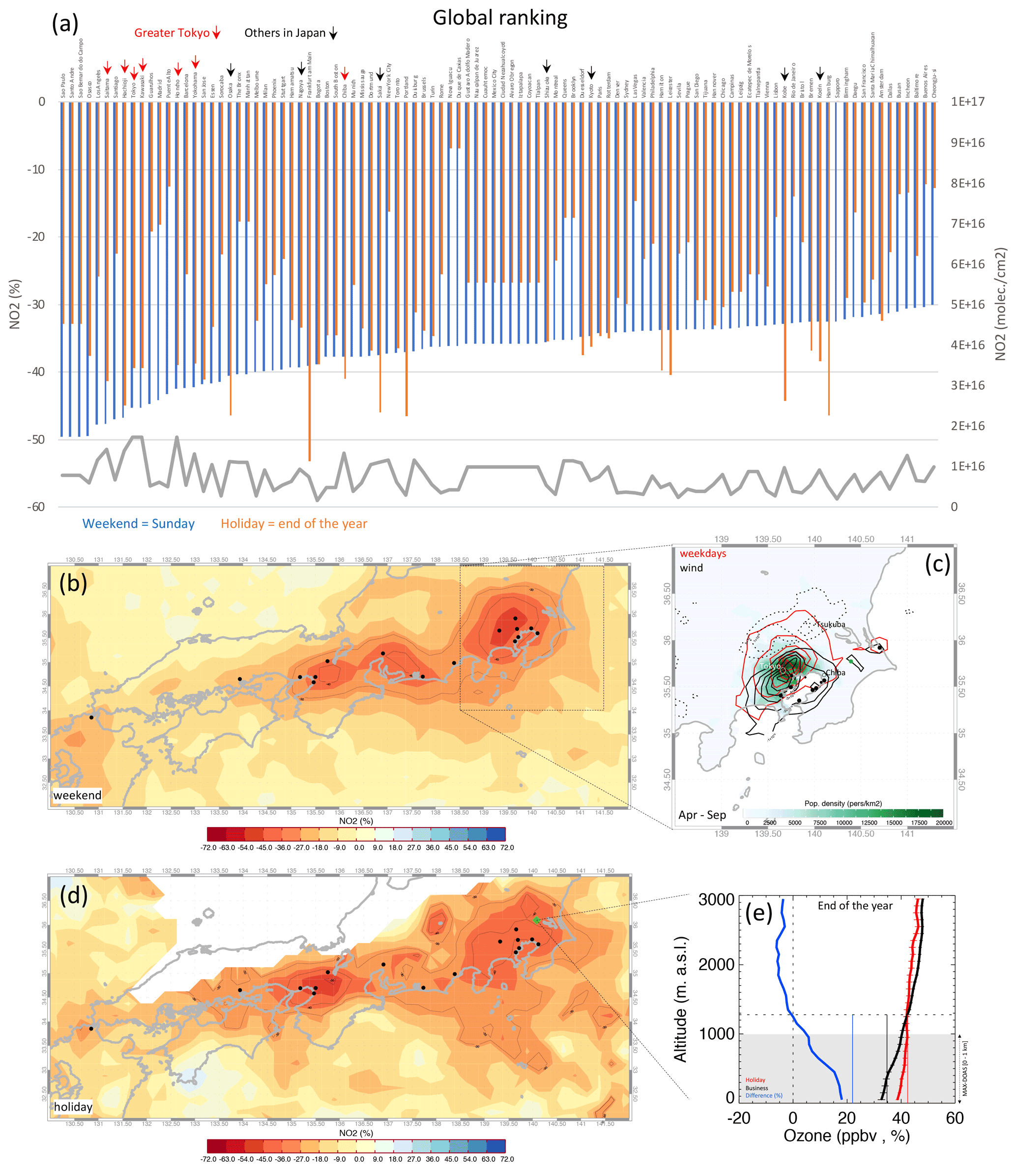
Figure 5Global ranking of the weekend effect (Sunday minus weekdays, blue) and holiday effect (end-of-year period minus business days, orange) for cities with a population greater than 0.5 million based on OMI NO2 in 2005–2019. Only cities where changes were larger than 30 % are shown. Opposite axis: mean NO2 total tropospheric column in grey (a). The spatial distribution of the weekend effect over Japan (b, relative changes) and over the Kanto region (c, absolute changes limited to April–September; red lines: Sunday minus weekdays; black points: power plants; green points: airports). Wind-related NO2 changes limited to April–September (black lines: high minus low wind speed) and population density (filled contours, in green shades) are also plotted in panel (c). Contours for both red and black solid lines read as follows: , , , , , molec. cm−2. Then, the black dashed lines show positive changes (0.5×10¹⁵, 1×10¹⁵ molec. cm−2). Spatial distribution of the holiday effect in NO2 across Japan (d); the low number of OMI observations prevents determination of the difference along the coastline of the Sea of Japan. Ozone profiles obtained from ozonesondes launched from Tateno (green point in d) during the end-of-year holiday period and business holidays in 2013–2020 (i.e., when MAX-DOAS data were available) are plotted along with box simulations (vertical lines) of the mean ozone concentration within the boundary layer (e). See Sect. 2 for further details.
Power plants and other industrial facilities are the dominant stationary emissions sources and are generally consistent, with little effect of weekly modulation. Satellite NO2 data can be used to investigate both stationary (Beirle et al., 2019) and mobility-related emissions sources (Ialongo et al., 2020). Using satellite NO2 and wind field data, emissions related to large and isolated stationary sources can be assessed (Beirle et al., 2019). Nevertheless, when multiple stationary sources are located within an urbanized region, as in our study area, evaluating the impacts of the various sources becomes challenging. As shown in Fig. 5c, we exploited the high resolution of TROPOMI data to compare NO2 changes associated with the weekly cycle (i.e., Sunday minus weekdays, red contours) to NO2 changes associated with wind speed (high wind speed days minus low wind speed days, black contours; see Sect. 2.2 for further details) in 2019–2020. Moreover, to better highlight the spatial patterns of these changes, we focused on the extended summer period from April to September, when the NO2 lifetime is shorter and NO2 tracks emissions sources better. Both contour lines suggest larger reductions over Tokyo than other areas, with patterns mostly matching the spatial distribution of population density. The weekly related NO2 generally extends north to Tsukuba and east to Chiba with a roughly homogeneous spatial gradient, while the gradient sharpens south of Chiba.
During days characterized by stagnant wind conditions, NO2 levels tend to accumulate around stationary sources, while rapid transport occurs with stronger winds. In addition to covering areas with a high population density, high negative wind-related changes are apparent around the main power plants on both sides of Tokyo Bay. Moreover, detailed distributions around stationary sources have been revealed (e.g., changes around Narita international airport and the isolated Kashima power plant on the east coast of Chiba Peninsula). Overall, the distribution of wind-related changes is more southerly than the bulk of weekly changes. Moreover, this gradient becomes positive in the north, highlighting the region downwind of the Tokyo area, including Tsukuba. Overall, wind-related NO2 changes closely resemble the pattern shown in the Japanese Emission Inventory.
The map in Fig. 5d shows the NO2 decrease occurring during the end-of-year holiday, when most anthropogenic emissions are reduced. To quantify this holiday effect, the average NO2 value of the 10 d before and after the holiday (defined here as the period from 25 December to 4 January) was subtracted from the holiday mean. Figure 5d shows patterns similar to Fig. 5b, although the longer NOx lifetime in winter causes the changes to be less confined to urbanized regions. TROPOMI NO2 decreased by about −43 % and −49 % in Chiba and Tsukuba, respectively (Fig. S2). The holiday effect is apparent in almost all cities with intense weekly cycles (Fig. 5a) and will be used as a further reference.
Multiyear MAX-DOAS observations of partial column NO2 recorded at Chiba University also showed a decrease around the end of the year (Fig. S2). It was about −44 %, while smaller changes occurred in HCHO (about −15 %). Slightly larger reductions were observed at the Tsukuba site (−55 % and 29 % for NO2 and HCHO, respectively).
Focusing on the holiday period provides insights into the response of O3 to these significant changes. As only data at SZA lower than 50∘ can be used to retrieve O3 with the DOAS method (Irie et al., 2011; see Sect. 2), we focused on ozonesonde profiles recorded at the Tateno Observatory, located about 50 km from Chiba. In this manner, we assessed the vertical distribution of O3 changes within and slightly above the PBL. These data were used to better interpret the changes in partial column O3 estimated by the MAX-DOAS systems. In the lower troposphere, the average O3 profile concentration averaged across business days was smaller than the O3 concentration recorded during the end-of-year holiday (Fig. 5e). The difference was greatest in the lowest layers (about −18 %) and remained nearly constant up to 0.5 km; then, it became smaller and disappeared above 1 km. The reduced NO titration effect occurring under VOC-limited conditions is likely the main driver of this peculiar pattern of increased O3 levels in the lowest layers during the holiday period.
We simulated the periods of 2019 and 2020 with the CLASS model using the appropriate mean NO2 and HCHO observations as well as lidar-based PBLH recorded at Chiba as initial conditions. The results of the simulations (vertical lines in Fig. 5e) confirmed the holiday-associated positive O3 enhancement, with a relative difference of 22 % at 15:00 LT, which was also the time of the sonde launch corresponding to the diurnal ozone peak. Previous studies have reported comparable O3 enhancement effects on the weekend, particularly in winter (Sadanaga et al., 2012; Sicard et al., 2020a). Using the same approach, we evaluated the changes occurring around mid-August, which is a period of reduced mobility. Such changes are interesting in terms of the O3 formation regime, but significant variability prevented clear identification of trends (Fig. S2).
Figure 6 further characterizes the NO2 weekend effect and contextualizes the holiday effect through comparison of ground-based partial column (<1 km), satellite-based tropospheric column, and surface in situ observations. In Chiba, relocation of all four instruments occurred in 2014 (i.e., the pointing direction of some sensors was changed slightly; Irie et al., 2021); therefore, in the following analysis, we exclude observations recorded in 2013 and 2014. Panel (a) shows the geographic distribution of NO2 weekly changes on Sunday for OMI, with MAX-DOAS and in situ observations plotted together. We focused on 2015–2018, when all three datasets were available. The spatial distribution of OMI NO2 is as shown in Fig. 5b. The largest negative changes occurred over Tokyo, which reached −45 %, and changes became smaller toward Chiba and Tsukuba. Notably, the magnitude of these changes is larger around Tsukuba (−35 %) than around Chiba (−30 %), although Tsukuba is a suburban site, while the urban area of Chiba hosts a larger population (Fig. 2) and industrial activities. In situ observations match the satellite-based spatial distribution, although with a somewhat smaller magnitude (by about 5 %).
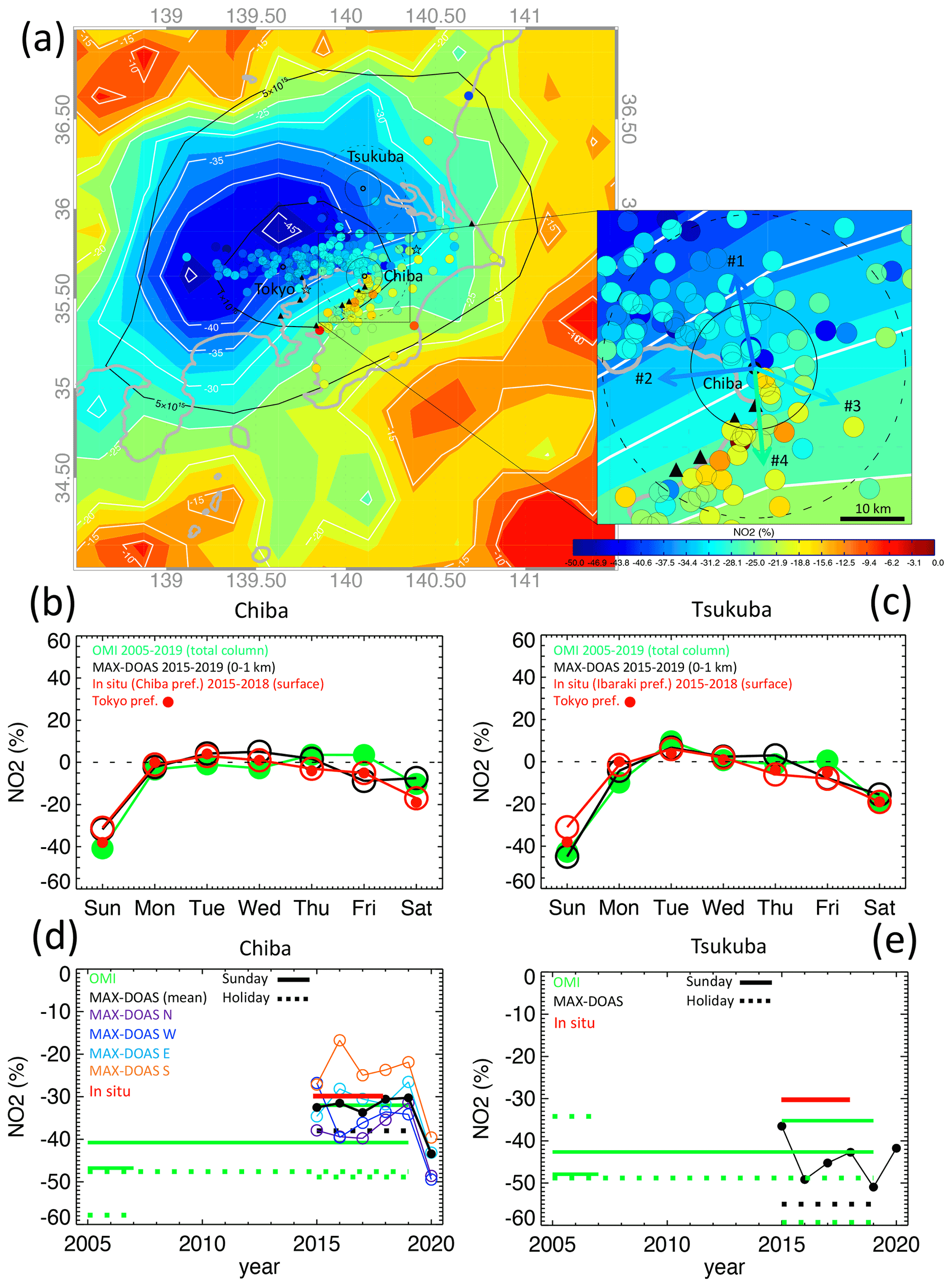
Figure 6Spatial distribution of the weekend effect (Sunday minus weekdays) based on OMI NO2 total tropospheric column (filled contours), MAX-DOAS partial tropospheric column (<1 km, colored arrows), and in situ NO2 observations (circles) over 2015–2018 (a, main panel). Magnified view of the area around Chiba University (inset). NO2 weekly cycle at Chiba and Tsukuba for the datasets noted above. In situ data were averaged across the prefecture (b, c). The weekend effect (on Sunday) and the holiday effect (at the end of the year) were averaged over different periods (as indicated by the horizontal lines) at Chiba and Tsukuba (d, e). MAX-DOAS NO2 data are also plotted for each year and for each instrument at Chiba.
MAX-DOAS partial column data reproduced the spatial distribution of the previous datasets (inset in Fig. 6a), showing a magnitude of change slightly closer to that of OMI (i.e., total column) than the surface network. Both in situ and MAX-DOAS observations were averaged over 09:00–15:00, while OMI observations were generally recorded around 13:30. The small incongruence among measurements is likely due to the different sampling periods (i.e., while in situ observations include data recorded under all meteorological conditions, satellite and MAX-DOAS data were limited to clear-sky days).
We also compared the climatology of the weekly cycle from various platforms according to data availability (excluding 2020). For comparison with the other datasets, we used the mean value from the in situ stations within Chiba (Fig. 6b) and Ibaraki (Fig. 6c) prefectures, respectively. Despite the different periods analyzed, the weekly cycles were very similar for all three platforms. The magnitude of change is largest on Sunday; at Chiba, OMI changes are approximately 10 % larger than both ground observation types. By contrast, at Tsukuba, in situ data are lower than OMI and MAX-DOAS by 10 %–15 % (but due to the scarcity of in situ stations around Tsukuba, the average value of stations inside Ibaraki prefecture is likely not representative of the area around Tsukuba). In addition to Sunday, indications of reduced NO2 are apparent on Friday and Saturday at both sites. As a further reference, we included the NO2 weekly cycle of Tokyo prefecture. The data confirmed that weekly cycles are similar in the three prefectures, with values for Tokyo on Sundays being about 5 %–10 % larger than in other prefectures.
Figure 6d and e show changes in OMI NO2 on Sunday averaged over the periods of 2005–2007, 2015–2019, and 2005–2019 at Chiba and Tsukuba. The OMI NO2 column over the investigated region decreased by about 50 % over 2005–2019 (see Fig. S3 for Chiba). Therefore, in accordance with a previous study (Stavrakou et al., 2020), the weekly cycle showed a reduced amplitude in recent years. During this latest period, in situ, satellite, and MAX-DOAS observations at Chiba coincided, while these data sources showed a spread of about 15 % at Tsukuba. This larger variability at Tsukuba is likely due to its lower NO2 levels and suburban location downwind of the Tokyo area (Fig. 5c).
As a further reference, Fig. 6d and e also show the end-of-year holiday reductions. Overall, when considering the full 2005–2019 period, OMI holiday changes were larger than OMI Sunday changes by about 8 % for both Chiba and Tsukuba. However, in recent years, NO2 values were much larger on holidays than on Sundays.
For Chiba, the distinct Sunday changes recorded by each of the four MAX-DOAS instruments were also investigated. The instruments showed a spread of less than 10 % with limited interannual variability. The amplitude of the NO2 weekend effect differed among instruments, with smaller effects for the instruments pointing south and east than for those pointing north and west. This difference was likely due to the presence of power plants and industrial activities within a few tens of kilometers south of the sampling site, providing an additional and more constant emissions source that reduces the difference between rest and business days. Indeed, absolute NO2 amounts were generally higher for the MAX-DOAS facing south, followed by the east-, west-, and finally north-facing instruments (inset in Fig. S3).
Moreover, changes in MAX-DOAS NO2 were much more prominent in 2020 than in previous years. Notably, 2020 was equally anomalous for all instruments, with decreases around 15 %–20 %. Therefore, the observed decrease was not a local phenomenon. Generally, MAX-DOAS changes at Tsukuba are more significant than the data recorded at Chiba. Nevertheless, at Tsukuba, changes in 2020 were within the usual level of interannual variability. Therefore, the anomalous weekly cycle in 2020 affected the urban region of Chiba but not the suburban area.
3.3 Weekly cycles
3.3.1 Weekly cycle of partial column NO2, HCHO, O3 and light-absorbing aerosols
Figure 7 shows the interannual weekly changes in MAX-DOAS partial columns of NO2, HCHO, O3, and at the Chiba and Tsukuba sites. Further changes in fAAOD (0–1 km) were reported for Chiba only. As we used observations averaged over four independent MAX-DOAS systems at Chiba, the data are more statistically robust and representative of a larger area than observations from Tsukuba (sampled with only one instrument). Therefore, most of the following discussion on interannual changes is focused on Chiba.
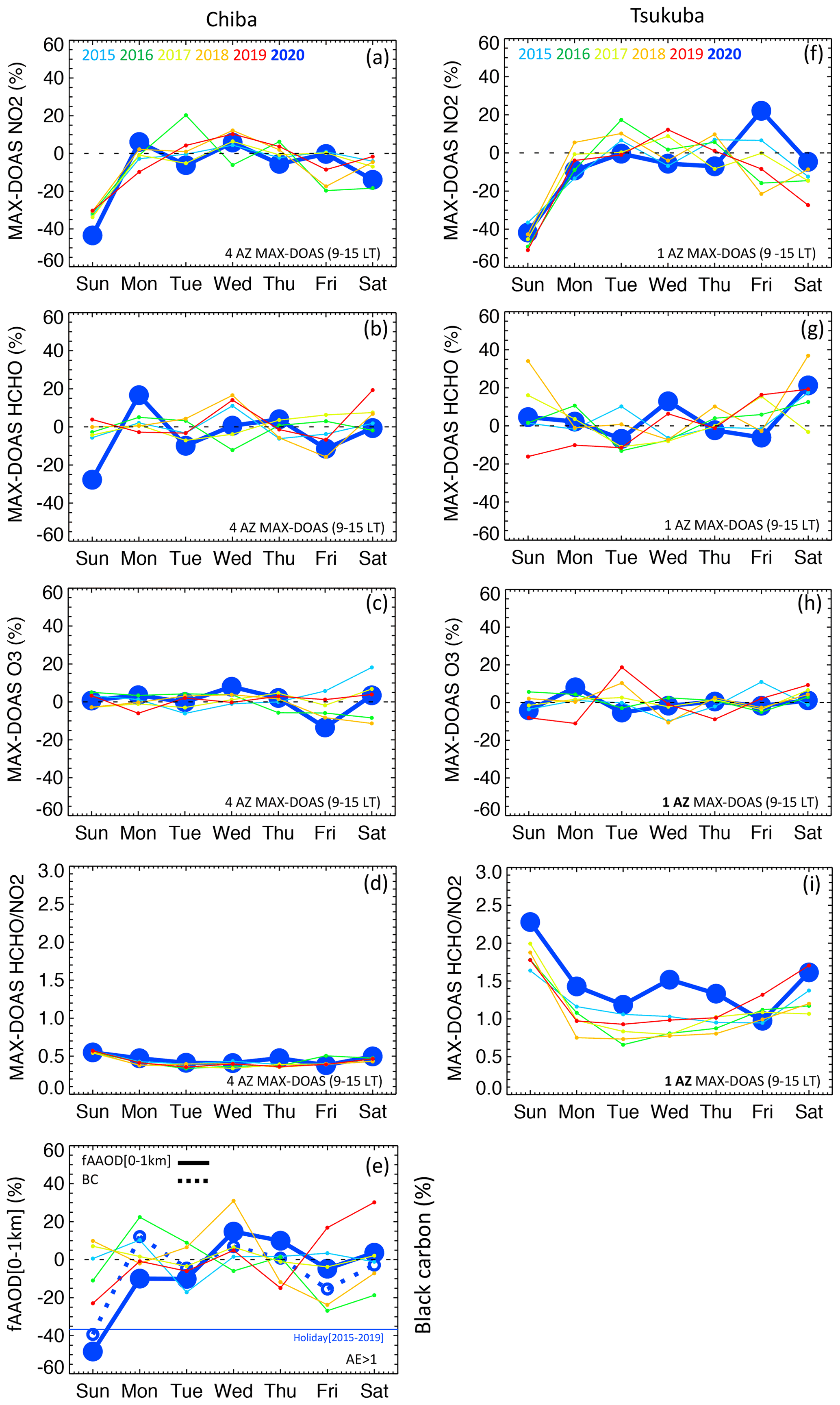
Figure 7Weekly changes in MAX-DOAS partial tropospheric column (top to bottom) NO2, HCHO, O3, , and fAAOD for Chiba (a–e) and Tsukuba (f–i) during 2015–2020. Only data with SZA < 50 were considered in the O3 dataset; see text for details. Panel (e) includes the weekly cycle of surface BC concentrations. BC data were unavailable for Tsukuba.
As noted above, at Chiba, while the NO2 change on Sunday was approximately −30 % for 2015–2019, it reached about −45 % in 2020. This difference was much larger than 2×σ (Fig. S4). On the other hand, except in 2020, interannual variability was much smaller on Sunday than on other days. By contrast, at Tsukuba, Sunday changes in 2020 were comparable to those in previous years.
Usually, the weekend effect was absent in HCHO data from both Chiba and Tsukuba. Nevertheless, at Chiba, negative HCHO changes on Sunday 2020 were unprecedentedly large (around −30 %). This negative anomaly is larger than the largest deviation on any other day in previous years and can be attributed to abnormally low anthropogenic NMVOC on the Sundays of 2020 (Sun et al., 2021; Ghahremanloo et al., 2021). By contrast, HCHO showed no unusual trends at Tsukuba in 2020, and this difference is likely due to differences in local conditions (i.e., Tsukuba is located in a suburban area, where a greater quantity of biogenic VOC emissions contribute to HCHO concentrations) and higher variability associated with the usage of only one instrument.
A weekly cycle in the ratio is evident for Tsukuba, with its peak on Sunday (approximately double the weekday average). On the other hand, for Chiba, the slightly higher ratio on Sunday was similar to the value on weekdays (0.55 vs. 0.4). Notably, on almost all days of 2020, the ratio at Tsukuba was higher than in previous years, while no difference was recorded at Chiba. Overall, due to the seasonal variations in NO2 and HCHO concentrations, the ratio also shows significant seasonality, with a large ratio in summer compared to the other seasons (Irie et al., 2021). Nevertheless, the frequent cloudy conditions in the late spring to summer period and the limited temporal extension of the dataset prevent evaluation of potential seasonal differences in its weekly cycle.
Despite this large variation in the main precursors, corresponding modulations in the O3 partial column were not recorded on Sundays of 2020 or previous years. Although the amplitude of the weekend effect in ozone is likely to have been reduced in recent years (Sicard et al., 2020a), its absence in our data contrasts with previous results showing a discernible weekend effect in surface ozone at Tokyo (Sadanaga et al., 2012). Ozone in the free troposphere presents a greatly smoothed diurnal cycle, if any, compared to surface ozone, and this diurnal cycle is generally strongest below 950 hPa (Petetin et al., 2016). The ozone profile is different from the other trace gases. In contrast to NO2, which strongly decreases its concentration with altitude, ozone concentration does not decrease with altitude. The ozone weekend effect at the surface level is usually 10 % (Sadanaga et al., 2012) and is much less evident than NO2. As suggested by ozonesonde observations (Fig. 5e), ozone changes due to titration maximize at the surface and tend to be reduced shortly at h>0.5 km. Since MAX-DOAS O3 partial column observations sample the 0–1 km layer, the effect tends to disappear in our data. Moreover, more titration is expected in winter, but MAX-DOAS O3 observations were unavailable this season (Sect. 2.1.1). Finally, the number of MAX-DOAS daily ozone samples was generally smaller than the other trace gases. Therefore, any potential weekly cycle would be difficult to observe in our MAX-DOAS O3 partial column dataset.
We further evaluated potential ozone differences between Sundays and weekdays of 2015–2020 using the box model (not shown). As in the previous simulations, we used MAX-DOAS observations of NO2 and HCHO as well as lidar-based PBLH as initial conditions and focused on the period most strongly affected by the pandemic (i.e., April–September). The simulated ozone differences between Sundays and weekdays were slightly negative (i.e., Sunday O3 < weekday O3) and ranged from −4 % in 2018 to −8 % in 2020.
As shown in the bottom panel, we examined the weekly cycle of fAAOD partial column data at Chiba. Although such data are characterized by high interannual variability, similar to the results presented above, 2020 data were anomalous and characterized by negative changes of about 50 % on Sunday with no variation on Saturday. Notably, consistent with the results for NO2 (Fig. 6d), changes in fAAOD on Sundays in 2020 are comparable with the effect usually observed during the end-of-year holiday. Although the weekly cycle is hardly discernible in the other years, the weekly cycle in 2020 is coherent with that of collocated observations of surface BC mass concentration, which show reductions larger than 40 % on Sunday and no change on Saturday.
We further excluded the influence of meteorology on the observed interannual variation by examining data on wind speed, wind direction, and temperature recorded at Chiba on days with available MAX-DOAS observations (Fig. S5). Overall, the results showed that wind did not drive the weekly changes in tropospheric gases. As increasing temperature enhances biogenic emissions and boosts oxidation processes, temperature is usually positively correlated with HCHO. We verified the absence of apparent weekly variation in temperature. Moreover, due to the large amount of data recorded at Chiba site, we could confirm that weekly changes around the satellite overpass time were representative of the daily NO2. No apparent difference between MAX-DOAS daily NO2 for 09:00–15:00 or 12:00–15:00 was observed (the same result was obtained for HCHO and O3).
3.3.2 Weekly cycle of TROPOMI NO2 tropospheric columns
Next, we examined the pattern of weekly changes in TROPOMI NO2, looking for differences in the spatial distribution and magnitude of Sunday changes between 2019 and 2020 (Fig. 8). Overall, changes were larger in 2020 than in 2019, reaching −50 % over central Tokyo. Moreover, during the extended summer period (April to September), when the largest influence of COVID is expected, differences between 2020 and 2019 were even more apparent. In addition to the magnitude of the differences, the area characterized by higher NO2 concentrations was greatly reduced in 2020 compared to 2019. This reduction averaged about −27 % for weekdays and reached −67 % for Sundays (Fig. S6).
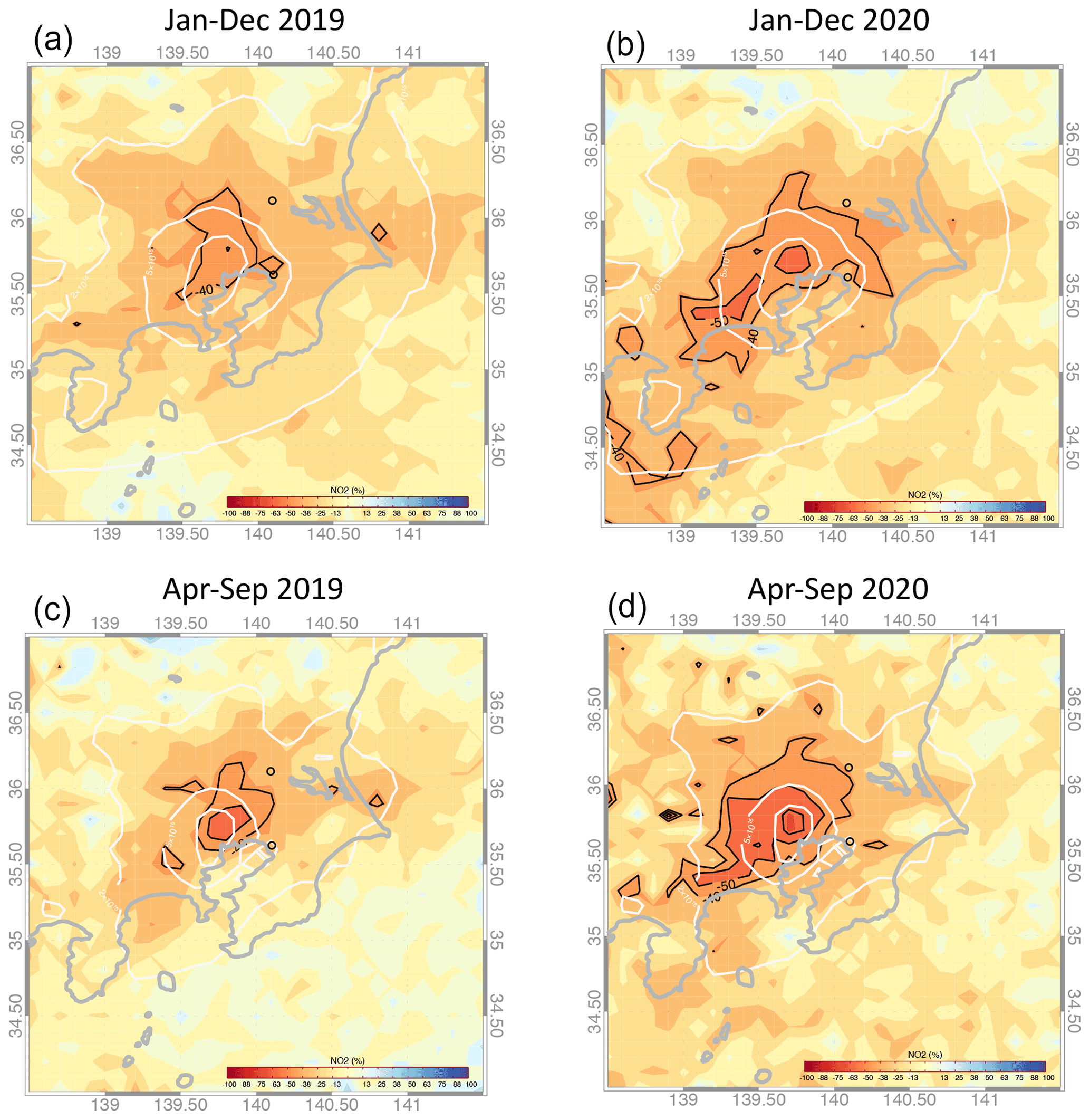
Figure 8Spatial distribution of the TROPOMI NO2 weekend effect (Sunday minus weekdays) in January to December 2019 (a), January to December 2020 (b), April to September 2019 (c), and April to September 2020 (d).
Within the areas sampled by the MAX-DOAS systems, TROPOMI showed no clear differences between 2019 and 2020 in either Chiba or Tsukuba. For Chiba, this contrasts with ground observations. Different time windows, over which the daily means were computed (i.e., between 09:00 and 15:00 for MAX-DOAS and around 13:30 for TROPOMI), and cloud screening procedures resulted in a larger amount of MAX-DOAS data than satellite data and likely contributed to these differences. However, despite being based on 1 year of observations, both TROPOMI maps could correctly reproduce the spatial pattern of changes estimated from ground-based observations around Chiba, i.e., the north–south gradient driven by the presence of power plants. This similarity provides confidence in identifying the interannual variability of the spatial distribution of the NO2 weekly cycle based on TROPOMI data.
This study investigated the interannual, seasonal, and weekly variabilities as well as spatial distributions in NO2, HCHO, O3, and light-absorbing aerosols measured with multiple platforms within the Greater Tokyo Area, which is the most populous metropolitan area in the world. We mainly examined the period of 2013–2020, focusing on 2020 when an effect from COVID-19 is expected. The main results can be summarized as follows.
-
In 2020, levels of NO2 and light-absorbing aerosols were the lowest on record, but the potential COVID-19 impact was superimposed on a decreasing trend.
-
At Chiba, MAX-DOAS observations within the PBL showed that annual NO2 reductions in 2020 were about 10 % relative to 2019, with limited changes during the period of the state of emergency. No deviations in O3 and HCHO were apparent.
-
TROPOMI column-based observations confirmed the observed reduction in NO2 and the absence of relevant changes in HCHO. During the state of emergency, NO2 reductions exceeded 40 % in the southern Tokyo area but were about 10 % over Chiba and Tsukuba. Moreover, both satellite and MAX-DOAS observations showed enhancement of the ratio, which was strongest in the suburban region.
-
OMI observations demonstrated that the weekly and holiday effects in NO2 within the GTA are among the largest in the world. NO2 reductions on rest days are not limited to the GTA but extend uniformly over most of Japan.
-
Surface in situ, MAX-DOAS partial column, and satellite-based tropospheric column observations showed a coherent NO2 weekly cycle, with the largest reductions on Sunday. Ground observations aligned with the spatial distribution of the satellite changes, even within the relatively limited area sampled by the MAX-DOAS systems.
-
In 2020, ground and satellite observations showed an anomalous weekly cycle in NO2 in urban areas, with larger reductions on Sunday than in previous years. Similar large changes in light-absorbing aerosols were identified. Such changes are comparable to the reductions observed during the end-of-year holiday period.
-
At Chiba, large NO2 reductions on Sunday were coupled with simultaneous reduction of HCHO, whereas no significant changes in O3 were observed.
-
In Japan, the reduction in mobility in 2020 was more extensive on the weekend than on business days, in accordance with the larger NO2 weekly change in 2020 found in the urban areas. By contrast, other countries generally showed the opposite behavior. This highlights modification of habits by the Japanese populace that resulted in unique air quality effects, suggesting widespread adoption of recommendations aimed at limiting the spread of the pandemic in Japan despite the lack of strict legal restrictions.
Although not explicitly mentioned in the previous discussion, an implicit assumption of our study relies on the fact that satellite observations available only around midday are representative of daily changes computed, for example, by hourly observations. Although we provide evidence that this is likely the case (see Fig. S5), data from new geostationary satellites (e.g., Geostationary Environment Monitoring Spectrometer on board the Geostationary Korea Multi-Purpose Satellite 2) are expected to shed some further light on this issue.
A further shortcoming is the scarcity of reliable satellite-based tropospheric ozone datasets to complement the satellite-based spatial distribution achieved with NO2 and HCHO observations. Despite the recent progress (Shen et al., 2019), OMI O3 only has some low sensitivity to the boundary layer, and this would make any analysis over the investigated region challenging (past studies found some correlation with the actual surface ozone in China, where tropospheric ozone is much larger; Shen et al., 2019). TROPOMI is expected to improve this capability soon, but its ozone dataset is currently limited to tropical latitudes.
Finally, it is worth mentioning the potential impact of the rebound of the long-range transport of pollutants after Chinese economic recovery from the COVID-19 pandemic (Itahashi et al., 2022) on the current pollution within the Kanto region, which will deserve further investigation.
All datasets used in the present study are publicly available as listed below.
-
https://www.temis.nl/ (TEMIS, 2021)
-
https://scihub.copernicus.eu/ (SCIHUB, 2021)
-
https://disc.gsfc.nasa.gov/ (DISC, 2021)
-
https://woudc.org/ (WOUDC, 2021)
-
https://www.google.com/covid19/mobility/ (Google Mobility, 2021)
-
http://atmos3.cr.chiba-u.jp/skynet/ (SKYNET, 2021)
-
http://atmos3.cr.chiba-u.jp/a-sky/ (A-SKY, 2021)
-
https://www.ecmwf.int/en/forecasts/dataset/cams-global-reanalysis (CAMS, 2021)
-
http://www.nies.go.jp/igreen/index.html (IGREEN, 2021)
The supplement related to this article is available online at: https://doi.org/10.5194/acp-22-12705-2022-supplement.
AD was responsible for conceptualization. AD and RCC developed the methodology. HI collected measurements and carried out data curation. AD, DAB, HMSH, and SK conducted analysis. HI acquired funding. AD, HI, DAB, and RRC contributed to writing (review and editing). All authors have read and agreed to the published version of the paper.
The contact author has declared that none of the authors has any competing interests.
Publisher's note: Copernicus Publications remains neutral with regard to jurisdictional claims in published maps and institutional affiliations.
The authors would like to thank the OMI and TROPOMI Science Teams for the data products, CAMS and MERRA-2 for the corresponding reanalysis data products, and JMA, AEROS, and NIES staff.
This research was supported by the Environment Research and Technology Development Fund (grant nos. JPMEERF20192001 and JPMEERF20215005) of the Environmental Restoration and Conservation Agency of Japan, JSPS KAKENHI (grant nos. JP19H04235, JP20H04320, JP22H03727, JP22H05004 and JP21K12227), the JAXA 2nd research announcement on the Earth Observations (grant no. 19RT000351), and the Virtual Laboratory (VL) project by the Ministry of Education, Culture, Sports, Science and Technology (MEXT), Japan. Raul R. Cordero was supported by the Consejo Nacional de Ciencias y Tecnología (CONICYT, Preis ANILLO ACT210046).
This paper was edited by Ilse Aben and reviewed by two anonymous referees.
Achakulwisut, P., Brauer, M., Hystad, P., and Anenberg, S. C.: Global, national, and urban burdens of paediatric asthma incidence attributable to ambient NO2 pollution: estimates from global datasets, Lancet Planet Health, 3, e166–e178, https://doi.org/10.1016/S2542-5196(19)30046-4, 2019.
Akimoto, H.: Overview of policy actions and observational data for PM2.5 and O3 in Japan: a study of urban air quality improvement in Asia, JICA-RI Working Paper, 137, https://www.jica.go.jp/jica-ri/publication/workingpaper/wp_137.html (last access: 26 September 2022), 2017.
A-SKY (International air quality and sky research remote sensing): A-SKY, http://atmos3.cr.chiba-u.jp/a-sky/, last access: 20 September 2021.
Barré, J., Petetin, H., Colette, A., Guevara, M., Peuch, V.-H., Rouil, L., Engelen, R., Inness, A., Flemming, J., Pérez García-Pando, C., Bowdalo, D., Meleux, F., Geels, C., Christensen, J. H., Gauss, M., Benedictow, A., Tsyro, S., Friese, E., Struzewska, J., Kaminski, J. W., Douros, J., Timmermans, R., Robertson, L., Adani, M., Jorba, O., Joly, M., and Kouznetsov, R.: Estimating lockdown-induced European NO2 changes using satellite and surface observations and air quality models, Atmos. Chem. Phys., 21, 7373–7394, https://doi.org/10.5194/acp-21-7373-2021, 2021.
Bauwens, M., Compernolle, S., Stavrakou, T., Müller, J.-F., van Gent, J., Eskes, H., Levelt, P. F., van der A, R., Veefkind, J. P., Vlietinck, J., Yu, H., and Zehner, C.: Impact of coronavirus outbreak on NO2 pollution assessed using TROPOMI and OMI observations, Geophys. Res. Lett., 47, e2020GL087978, https://doi.org/10.1029/2020GL087978, 2020.
Beirle, S., Platt, U., Wenig, M., and Wagner, T.: Weekly cycle of NO2 by GOME measurements: a signature of anthropogenic sources, Atmos. Chem. Phys., 3, 2225–2232, https://doi.org/10.5194/acp-3-2225-2003, 2003.
Beirle, S., Borger, C., Dörner, S., Li, A., Hu, Z., Liu, F., Wang, Y., and Wagner, T.: Pinpointing nitrogen oxide emissions from space, Sci. Adv., 5, eaax9800, https://doi.org/10.1126/sciadv.aax9800, 2019.
Brancher, M.: Increased ozone pollution alongside reduced nitrogen dioxide concentrations during Vienna's first COVID-19 lockdown: Significance for air quality management, Environ. Pollut., 284, 117153, https://doi.org/10.1016/j.envpol.2021.117153, 2021.
Buchard, V., Randles, C.A., Da Silva, A.M., Colarco, P.R., Darmenov, A., Govindaraju, R., Smirnov, A., Hoblen, B., Ferrare, R., Hair, J., Beyersdorf, A. J., Ziemba, L. D., and Yu, H.: The MERRA-2 Aerosol Reanalysis, 1980 Onward. Part II: Evaluation and Case Studies, J. Climate, 30, 6851–6872, https://doi.org/10.1175/JCLI-D-16-0613.1, 2017.
CAMS (Copernicus Atmosphere Monitoring Service): CAMS global reanalysis (EAC4), ECMWF [data set], https://www.ecmwf.int/en/forecasts/dataset/cams-global-reanalysis, last access: 9 September 2021.
Cleveland, W. S., Graedel, T. E., Kleiner, B., and Warner, J. L.: Sunday and workday variations in photochemical air pollutants in New Jersey and New York, Science, 186, 1037–1038, https://doi.org/10.1080/10473289.2003.10466222, 1974.
Compernolle, S., Verhoelst, T., Pinardi, G., Granville, J., Hubert, D., Keppens, A., Niemeijer, S., Rino, B., Bais, A., Beirle, S., Boersma, F., Burrows, J. P., De Smedt, I., Eskes, H., Goutail, F., Hendrick, F., Lorente, A., Pazmino, A., Piters, A., Peters, E., Pommereau, J.-P., Remmers, J., Richter, A., van Geffen, J., Van Roozendael, M., Wagner, T., and Lambert, J.-C.: Validation of Aura-OMI QA4ECV NO2 climate data records with ground-based DOAS networks: the role of measurement and comparison uncertainties, Atmos. Chem. Phys., 20, 8017–8045, https://doi.org/10.5194/acp-20-8017-2020, 2020.
Cooper, M. J., Martin, R. V., Hammer, M. S., Levelt, P. F., Veefkind, P., Lamsal, L. N., Krotkov, N. A., Brook, J. R., and McLinden, C. A.: Global fine-scale changes in ambient NO2 during COVID-19 lockdowns, Nature, 601, 380–387, https://doi.org/10.1038/s41586-021-04229-0, 2022.
Damiani, A., Irie, H., Yamaguchi, K., Hoque, H. M. S., Nakayama, T., Matsumi, Y., Kondo, Y., and Da Silva, A.: Variabilities in PM2.5 and black carbon surface concentrations reproduced by aerosol optical properties estimated by in-situ data, ground based remote sensing and modeling, Remote Sens., 13, 3163, https://doi.org/10.3390/rs13163163, 2021.
De Smedt, I., Theys, N., Yu, H., Danckaert, T., Lerot, C., Compernolle, S., Van Roozendael, M., Richter, A., Hilboll, A., Peters, E., Pedergnana, M., Loyola, D., Beirle, S., Wagner, T., Eskes, H., van Geffen, J., Boersma, K. F., and Veefkind, P.: Algorithm theoretical baseline for formaldehyde retrievals from S5P TROPOMI and from the QA4ECV project, Atmos. Meas. Tech., 11, 2395–2426, https://doi.org/10.5194/amt-11-2395-2018, 2018.
De Smedt, I., Pinardi, G., Vigouroux, C., Compernolle, S., Bais, A., Benavent, N., Boersma, F., Chan, K.-L., Donner, S., Eichmann, K.-U., Hedelt, P., Hendrick, F., Irie, H., Kumar, V., Lambert, J.-C., Langerock, B., Lerot, C., Liu, C., Loyola, D., Piters, A., Richter, A., Rivera Cárdenas, C., Romahn, F., Ryan, R. G., Sinha, V., Theys, N., Vlietinck, J., Wagner, T., Wang, T., Yu, H., and Van Roozendael, M.: Comparative assessment of TROPOMI and OMI formaldehyde observations and validation against MAX-DOAS network column measurements, Atmos. Chem. Phys., 21, 12561–12593, https://doi.org/10.5194/acp-21-12561-2021, 2021.
DISC (GES DISC): DISC OMI, NASA [data set], https://disc.gsfc.nasa.gov/, last access: 30 September 2021.
Duncan, B. N., Yoshida, Y., Olson, J. R., Sillman, S., Martin, R. V., Lamsal, L., Hu, Y. T., Pickering, K. E., Retscher, C., Allen, D. J., and Crawford, J. H.: Application of OMI observations to a space-based indicator of NOx and VOC controls on surface ozone formation, Atmos. Environ., 44, 2213–2223, https://doi.org/10.1016/j.atmosenv.2010.03.010, 2010.
Fioletov, V., McLinden, C. A., Griffin, D., Krotkov, N., Liu, F., and Eskes, H.: Quantifying urban, industrial, and background changes in NO2 during the COVID-19 lockdown period based on TROPOMI satellite observations, Atmos. Chem. Phys., 22, 4201–4236, https://doi.org/10.5194/acp-22-4201-2022, 2022.
Geddes, J. A., Martin, R. V., Boys, B. L., and van Donkelaar, A.: Long-term trends worldwide in ambient NO2 concentrations inferred from satellite observations, Environ. Health Persp., 124, 281–289, https://doi.org/10.1289/ehp.1409567, 2016.
Georgoulias, A. K., van der A, R. J., Stammes, P., Boersma, K. F., and Eskes, H. J.: Trends and trend reversal detection in 2 decades of tropospheric NO2 satellite observations, Atmos. Chem. Phys., 19, 6269–6294, https://doi.org/10.5194/acp-19-6269-2019, 2019.
Ghahremanloo, M., Lops, Y., Choi, Y., and Mousavinezhad, S.: Impact of the COVID-19 outbreak on air pollution levels in East Asia, Sci. Total Environ., 754, 142226, https://doi.org/10.1016/j.scitotenv.2020.142226, 2021.
Gkatzelis, G. I., Gilman, J. B., Brown, S. S., Eskes, H., Gomes, A. R., Lange, A. C., McDonald, B. C., Peischl, J., Petzold, A., Thompson, C. R., and Kiendler-Scharr, A.: The global impacts of COVID-19 lockdowns on urban air pollution: A critical review and recommendations, Elementa: Science of the Anthropocene, 9, 00176, https://doi.org/10.1525/elementa.2021.00176, 2021.
Google Mobility (COVID-19 Community Mobility Reports): Community Mobility Reports, Google [data set], https://www.google.com/covid19/mobility/, last access: 20 September 2021.
Guevara, M., Jorba, O., Soret, A., Petetin, H., Bowdalo, D., Serradell, K., Tena, C., Denier van der Gon, H., Kuenen, J., Peuch, V.-H., and Pérez García-Pando, C.: Time-resolved emission reductions for atmospheric chemistry modelling in Europe during the COVID-19 lockdowns, Atmos. Chem. Phys., 21, 773–797, https://doi.org/10.5194/acp-21-773-2021, 2021.
Hamra, G. B., Laden, F., Cohen, A. J., Raaschou-Nielsen, O., Brauer, M., and Loomis, D.: Lung Cancer and Exposure to Nitrogen Dioxide and Traffic: A Systematic Review and Meta-Analysis, Environ. Health Persp., 123, 11, 1107–1112, https://doi.org/10.1289/ehp.1408882, 2015.
Hönninger, G., von Friedeburg, C., and Platt, U.: Multi axis differential optical absorption spectroscopy (MAX-DOAS), Atmos. Chem. Phys., 4, 231–254, https://doi.org/10.5194/acp-4-231-2004, 2004.
Ialongo, I., Virta, H., Eskes, H., Hovila, J., and Douros, J.: Comparison of TROPOMI/Sentinel-5 Precursor NO2 observations with ground-based measurements in Helsinki, Atmos. Meas. Tech., 13, 205–218, https://doi.org/10.5194/amt-13-205-2020, 2020.
IGREEN: IGREEN, NIES [data set], http://www.nies.go.jp/igreen/index.html, last access: 30 September 2021.
Inness, A., Ades, M., Agustí-Panareda, A., Barré, J., Benedictow, A., Blechschmidt, A.-M., Dominguez, J. J., Engelen, R., Eskes, H., Flemming, J., Huijnen, V., Jones, L., Kipling, Z., Massart, S., Parrington, M., Peuch, V.-H., Razinger, M., Remy, S., Schulz, M., and Suttie, M.: The CAMS reanalysis of atmospheric composition, Atmos. Chem. Phys., 19, 3515–3556, https://doi.org/10.5194/acp-19-3515-2019, 2019.
Irie, H., Takashima, H., Kanaya, Y., Boersma, K. F., Gast, L., Wittrock, F., Brunner, D., Zhou, Y., and Van Roozendael, M.: Eight-component retrievals from ground-based MAX-DOAS observations, Atmos. Meas. Tech., 4, 1027–1044, https://doi.org/10.5194/amt-4-1027-2011, 2011.
Irie, H., Nakayama, T., Shimizu, A., Yamazaki, A., Nagai, T., Uchiyama, A., Zaizen, Y., Kagamitani, S., and Matsumi, Y.: Evaluation of MAX-DOAS aerosol retrievals by coincident observations using CRDS, lidar, and sky radiometer inTsukuba, Japan, Atmos. Meas. Tech., 8, 2775–2788, https://doi.org/10.5194/amt-8-2775-2015, 2015.
Irie, H., Yonekawa, D., Damiani, A., Hoque, H. M. S., Sudo, K., and Itahashi, S.: Continuous multi-component MAX-DOAS observations for the planetary boundary layer ozone variation analysis at Chiba and Tsukuba, Japan, from 2013 to 2019, Prog. Earth Planet. Sci., 8, 31, https://doi.org/10.1186/s40645-021-00424-9, 2021.
Itahashi, S., Yamamura, Y., Wang, Z., and Uno, I.: Returning long-range PM2.5 transport into the leeward of East Asia in 2021 after Chinese economic recovery from the COVID-19 pandemic, Sci. Rep.-UK, 12, 5539, https://doi.org/10.1038/s41598-022-09388-2, 2022., 2022.
Jin, X., Fiore, A. M., Murray, L. T., Valin, L. C., Lamsal, L. N., Duncan, B., Boersma, K. F., De Smedt, I., Abad, G. G., Chance, K., and Tonnesen, G.: Evaluating a space-based indicator of surface ozone-NOx-VOC sensitivity over midlatitude source regions and application to decadal trends, J. Geophys. Res., 122, 10439–10461, https://doi.org/10.1002/2017JD026720, 2017.
Ju, M. J., Oh, J., and Choi, Y. H.: Changes in air pollution levels after COVID-19 outbreak in Korea, Sci. Total Environ., 750, 141521, https://doi.org/10.1016/j.scitotenv.2020.141521, 2021.
Kondo, Y., Sahu, L., Kuwata, M., Miyazaki, Y., Takegawa, N., Moteki, N., Imaru, J., Han, S., Nakayama, T., Kim Oanh, N. T., Hu, M., Kim, Y. J., and Kita, K.: Stabilization of the mass absorption cross section of black carbon for filter-based absorption photometry by the use of a heated inlet, Aerosol Sci. Tech., 43, 741–756, 2009.
Kurokawa, J. and Ohara, T.: Long-term historical trends in air pollutant emissions in Asia: Regional Emission inventory in ASia (REAS) version 3, Atmos. Chem. Phys., 20, 12761–12793, https://doi.org/10.5194/acp-20-12761-2020, 2020.
Lamsal, L. N., Krotkov, N. A., Vasilkov, A., Marchenko, S., Qin, W., Yang, E.-S., Fasnacht, Z., Joiner, J., Choi, S., Haffner, D., Swartz, W. H., Fisher, B., and Bucsela, E.: Ozone Monitoring Instrument (OMI) Aura nitrogen dioxide standard product version 4.0 with improved surface and cloud treatments, Atmos. Meas. Tech., 14, 455–479, https://doi.org/10.5194/amt-14-455-2021, 2021.
Laughner, J. L., Neu, J. L., Schimel, D., Wennberg, P. O., Barsanti, K., Bowman, K. W., Chatterjee, A., Croes, B. E., Fitzmaurice, H. L., Henze, D. K., Kim, J., Kort, E. A., Liu, Z., Miyazaki, K., Turner, A. J., Anenberg, S., Avise, J., Caok, H., Crisp, D., de Gouw, J., Eldering, A., Fyfer, J. C., Goldberg, D. L., Gurney, K. R., Hasheminassab, S., Hopkins, F., Iveyd, C. E., Jones, D., B. A., Liu, J., Lovenduski, N. S., Martin, R. V., McKinley, G. A., Ott, L., Poultera, B., Ru, M., Sander, S. P., Swart, N., Yung, Y. L., Zeng, Z.-C., and the rest of the Keck Institute for Space Studies “COVID-19: Identifying Unique Opportunities for Earth System Science” study team: Societal shifts due to COVID-19 reveal large-scale complexities and feedbacks between atmospheric chemistry and climate change, P. Natl. Acad. Sci. USA, 118, e2109481118, https://doi.org/10.1073/pnas.2109481118, 2021.
Le, T., Wang, Y., Liu, L., Yang, J., Yung, Y. L., Li, G., and Seinfeld, J. H.: Unexpected air pollution with marked emission reductions during the COVID-19 outbreak in China, Science, 369, 702–706, https://doi.org/10.1126/science.abb7431, 2020.
Lee, H.-J., Chang, L.-S., Jaffe, D. A., Bak, J., Liu, X., Abad, G. G., Jo, H.-Y., Jo, Y.-J., Lee, J.-B., and Kim, C.-H.: Ozone Continues to Increase in East Asia Despite Decreasing NO2: Causes and Abatements, Remote Sens., 13, 11, 2177, https://doi.org/10.3390/rs13112177, 2021.
Levelt, P. F., Stein Zweers, D. C., Aben, I., Bauwens, M., Borsdorff, T., De Smedt, I., Eskes, H. J., Lerot, C., Loyola, D. G., Romahn, F., Stavrakou, T., Theys, N., Van Roozendael, M., Veefkind, J. P., and Verhoelst, T.: Air quality impacts of COVID-19 lockdown measures detected from space using high spatial resolution observations of multiple trace gases from Sentinel-5P/TROPOMI, Atmos. Chem. Phys., 22, 10319–10351, https://doi.org/10.5194/acp-22-10319-2022, 2022.
Li, K., Jacob, D. J., Liao, H., Shen, L., Zhang, Q., and Bates, K. H.: Anthropogenic drivers of 2013–2017 trends in summer surface ozone in China, P. Natl. Acad. Sci USA, 116, 422–427, https://doi.org/10.1073/pnas.1812168116, 2019.
Liu, F., Beirle, S., Zhang, Q., Dörner, S., He, K., and Wagner, T.: NOx lifetimes and emissions of cities and power plants in polluted background estimated by satellite observations, Atmos. Chem. Phys., 16, 5283–5298, https://doi.org/10.5194/acp-16-5283-2016, 2016.
Liu, Y., Wang, T., Stavrakou, T., Elguindi, N., Doumbia, T., Granier, C., Bouarar, I., Gaubert, B., and Brasseur, G. P.: Diverse response of surface ozone to COVID-19 lockdown in China, Sci. Total Environ., 789, 147739, https://doi.org/10.1016/j.scitotenv.2021.147739, 2021.
Martin, R. V., Fiore, A. M., and Van Donkelaar, A.: Space-based diagnosis of surface ozone sensitivity to anthropogenic emissions, Geophys. Res. Lett., 31, L06120, https://doi.org/10.1029/2004GL019416, 2004.
Murphy, J. G., Day, D. A., Cleary, P. A., Wooldridge, P. J., Millet, D. B., Goldstein, A. H., and Cohen, R. C.: The weekend effect within and downwind of Sacramento – Part 1: Observations of ozone, nitrogen oxides, and VOC reactivity, Atmos. Chem. Phys., 7, 5327–5339, https://doi.org/10.5194/acp-7-5327-2007, 2007.
Miyazaki, K., Bowman, K., Sekiya, T., Takigawa, M., Neu1, J. L., Sudo, K., Osterman, G., and Eskes, H.: Global tropospheric ozone responses to reduced NOx emissions linked to the COVID-19 worldwide lockdowns, Sci. Adv., 7, 24, https://doi.org/10.1126/sciadv.abf7460, 2021.
Nouvellet, P., Bhatia, S., Cori, A., Ainslie, K. E. C., Baguelin, M., Bhatt, S., Boonyasiri, A., Brazeau, N. F., Cattarino, L., Cooper, L. V., Coupland, H., Cucunuba, Z. M., Cuomo-Dannenburg, G., Dighe, A., Djaafara, B. A., Dorigatti, I., Eales, O. D., van Elsland, S. L., Nascimento, F. F., FitzJohn, R. G., Gaythorpe, K. A. M., Geidelberg, L., Green, W. D., Hamlet, A., Hauck, K., Hinsley, W., Imai, N., Jeffrey, B., Knock, E., Laydon, D. J., Lees, J. A., Mangal, T., Mellan, T. A., Nedjati-Gilani, G., Parag, K. V., Pons-Salort, M., Ragonnet-Cronin, M., Riley, S., Unwin, H. J. T., Verity, R., Vollmer, M. A. C., Volz, E., Walker, P. G. T., Walters, C. E., Wang, H., Watson, O. J., Whittaker, C., Whittles, L. K., Xi, X., Ferguson, N. M., and Donnelly, C. A.: Reduction in mobility and COVID-19 transmission, Nat. Commun., 12, 1090, https://doi.org/10.1038/s41467-021-21358-2, 2021.
Petetin, H., Thouret, V., Athier, G., Blot, R., Boulanger, D., Cousin, J.-M., Gaudel, A., Nédélec, P., and Cooper, O.: Diurnal cycle of ozone throughout the troposphere over Frankfurt as measured by MOZAIC-IAGOS commercial aircraft, Elementa: Science of the Anthropocene, 4, 129, https://doi.org/10.12952/journal.elementa.000129, 2016.
Platt, U. and Stutz, J.: Differential optical absorption spectroscopy, principles and applications, Springer, XV, 597 pp., 272 illus., 29 in color, Physics of Earth and Space Environments, ISBN 978-3-540-21193-8, 2008.
Randles, C. A., da Silva, A. M., Buchard, V., Colarco, P. R., Darmenov, A., Govindaraju, R., Smirnov, A., Holben, B., Ferrare, R., Hair, J., Shinozuka, Y., and Flynn, C. J.: The MERRA-2 Aerosol Reanalysis, 1980 Onward. Part I: System Description and Data Assimilation Evaluation. J. Climate, 30, 6823–6850, https://doi.org/10.1175/JCLI-D-16-0609.1, 2017.
Russell, A. R., Valin, L. C., and Cohen, R. C.: Trends in OMI NO2 observations over the United States: effects of emission control technology and the economic recession, Atmos. Chem. Phys., 12, 12197–12209, https://doi.org/10.5194/acp-12-12197-2012, 2012.
Ryan, R. G., Rhodes, S., Tully, M., and Schofield, R.: Surface ozone exceedances in Melbourne, Australia are shown to be under NOx control, as demonstrated using formaldehyde: NO2 and glyoxal: formaldehyde ratios, Sci. Total Environ., 749, 141460, https://doi.org/10.1016/j.scitotenv.2020.141460, 2020.
Sadanaga, Y., Sengen, M., Takenaka, N., and Bandow, H.: Analyses of the Ozone Weekend Effect in Tokyo, Japan: Regime of Oxidant (O3 + NO2) Production, Aerosol Air Qual. Res., 12, 161–168, https://doi.org/10.4209/aaqr.2011.07.0102, 2012.
Schroeder, J. R., Crawford, J. H., Fried, A., Walega, J., Weinheimer, A., Wisthaler, A., Muller, M., Mikovinu, T., Chen, G., and Shook, M.: New insights into the column ratio as an indicator of near‐surface ozone sensitivity, J. Geophys. Res., 122, 8885–8907, https://doi.org/10.1002/2017JD026781, 2017.
SCIHUB (Copernicus Open Access Hub): Sentinel-5P TROPOMI, Copernicus [data set], https://scihub.copernicus.eu/, last access: 30 September 2021.
Shakil, M. H., Munim, Z. H., Tasnia, M., and Sarowar, S.: COVID-19 and the environment: A critical review and research agenda, Sci. Total Environ., 745, 141022, https://doi.org/10.1016/j.Scitotenv.2020.141022, 2020.
Shen, L., Jacob, D. J., Liu, X., Huang, G., Li, K., Liao, H., and Wang, T.: An evaluation of the ability of the Ozone Monitoring Instrument (OMI) to observe boundary layer ozone pollution across China: application to 2005–2017 ozone trends, Atmos. Chem. Phys., 19, 6551–6560, https://doi.org/10.5194/acp-19-6551-2019, 2019.
Sicard, P., Paoletti, E., Agathokleous, E., Araminienė, V., Proietti, C., Coulibaly, F., and De Marco, A.: Ozone weekend effect in cities: Deep insights for urban air pollution control, Environ. Res., 191, 110193, https://doi.org/10.1016/j.envres.2020.110193, 2020a.
Sicard, P., De Marco, A., Agathokleous, E., Feng, Z., Xu, X., Paoletti, E., Diéguez Rodriguez, J. J., and Calatayud, V.: Amplified ozone pollution in cities during the COVID-19 lockdown, Sci. Total Environ., 735, 139542, https://doi.org/10.1016/j.scitotenv.2020.139542, 2020b.
Sillman, S.: The use of NOy, H2O2, and HNO3 as indicators for Ozone-NOx-Hydrocarbon sensitivity in urban Locations, J. Geophys. Res.-Atmos., 100, 14175–14188, https://doi.org/10.1029/94jd02953, 1995.
SKYNET: SKYNET CEReS Chiba University, SKYNET [data set], http://atmos3.cr.chiba-u.jp/skynet/, last access: 20 September 2021.
Stavrakou, T., Müller, J.-F., Bauwens, M., Boersma, K. F., and van Geffen, J.: Satellite evidence for changes in the NO2 weekly cycle over large cities, Sci. Rep.-UK, 10, 10066, https://doi.org/10.1038/s41598-020-66891-0, 2020.
Stein, O., Schultz, M. G., Bouarar, I., Clark, H., Huijnen, V., Gaudel, A., George, M., and Clerbaux, C.: On the wintertime low bias of Northern Hemisphere carbon monoxide found in global model simulations, Atmos. Chem. Phys., 14, 9295–9316, https://doi.org/10.5194/acp-14-9295-2014, 2014.
Steinbrecht, W., Kubistin, D., Plass-Dülmer, C., Davies, J., Tarasick, D. W., Gathen, P., Deckelmann, H., Jepsen, N., Kivi, R., Lyall, N., Palm, M., Notholt, J., Kois, B., Oelsner, P., Allaart, M., Piters, A., Gill, M., Van Malderen, R., Delcloo, A. W., Sussmann, R., Mahieu, E., Servais, C., Romanens, G., Stübi, R., Ancellet, G., Godin-Beekmann, S., Yamanouchi, S., Strong, K., Johnson, B., Cullis, P., Petropavlovskikh, I., Hannigan, J. W., Hernandez, J.-L., Diaz Rodriguez, A., Nakano, T., Chouza, F., Leblanc, T., Torres, C., Garcia, O., Röhling, A. N., Schneider, M., Blumenstock, T., Tully, M., Paton-Walsh, C., Jones, N., Querel, R., Strahan, S., Stauffer, R. M., Thompson, A. M., Inness, A., Engelen, R., Chang, K.-L., and Cooper, O. R.: COVID-19 crisis reduces free tropospheric ozone across the Northern Hemisphere, Geophys. Res. Lett., 48, e2020GL091987, https://doi.org/10.1029/2020GL091987, 2021.
Sugawara, H., Ishidoya, S., Terao, Y., Takane, Y., Kikegawa, Y., and Nakajima, K.: Anthropogenic CO2 emissions changes in an urban area of Tokyo, Japan, due to the COVID-19 pandemic: A case study during the state of emergency in April–May 2020, Geophys. Res. Lett., 48, e2021GL092600, https://doi.org/10.1029/2021GL092600, 2021.
Sun, W., Zhu, L., De Smedt, I., Bai, B., Pu, D., Chen, Y., Shu, L., Wang, D., Fu, T.-M., Wang, X., and Yang, X.: Global significant changes in formaldehyde (HCHO) columns observed from space at the early stage of the COVID-19 pandemic, Geophys. Res. Lett., 48, e2020GL091265, https://doi.org/10.1029/2020GL091265, 2021.
Surl, L., Palmer, P. I., and González Abad, G.: Which processes drive observed variations of HCHO columns over India?, Atmos. Chem. Phys., 18, 4549–4566, https://doi.org/10.5194/acp-18-4549-2018, 2018.
Tan, P.-H., Chou, C., Liang, J.-Y., Chou, C. C.-K., and Shiu, C.-J.: Air pollution “holiday effect” resulting from the Chinese New Year, Atmospheric Environment, 43, 2114-2124, https://doi.org/10.1016/j.atmosenv.2009.01.037, 2009.
Takane, Y., Nakajima, K., and Kikegawa, Y.: Urban climate changes during the COVID-19 pandemic: integration of urban-building-energy model with social big data, npj Clim. Atmos. Sci., 5, 44, https://doi.org/10.1038/s41612-022-00268-0, 2022.
Takashima, H., Irie, H., Kanaya, Y., Shimizu, A., Aoki, K., and Akimoto, H.: Atmospheric aerosol variations at Okinawa Island in Japan observed by MAX-DOAS using a new cloud screening method, J. Geophys. Res., 114, D18213, https://doi.org/10.1029/2009JD011939, 2009.
TEMIS (Tropospheric Emission Monitoring Internet Service): TEMIS TROPOMI (TM5-MP-DOMINO), TEMIS [data set], https://www.temis.nl/, last access: 15 September 2021.
van Geffen, J. H. G. M., Eskes, H. J., Boersma, K. F., and Veefkind, J. P.: TROPOMI ATBD of the total and tropospheric NO2 data products, Report S5P-KNMI-L2-0005-RP, KNMI, De Bilt, the Netherlands, https://sentinel.esa.int/documents/247904/2476257/Sentinel-5P-TROPOMI-ATBD-NO2-data-products, last access: 23 September 2022.
van Stratum, B. J. H., Vilà-Guerau de Arellano, J., Ouwersloot, H. G., van den Dries, K., van Laar, T. W., Martinez, M., Lelieveld, J., Diesch, J.-M., Drewnick, F., Fischer, H., Hosaynali Beygi, Z., Harder, H., Regelin, E., Sinha, V., Adame, J. A., Sörgel, M., Sander, R., Bozem, H., Song, W., Williams, J., and Yassaa, N.: Case study of the diurnal variability of chemically active species with respect to boundary layer dynamics during DOMINO, Atmos. Chem. Phys., 12, 5329–5341, https://doi.org/10.5194/acp-12-5329-2012, 2012.
Veefkind, J. P., Aben, I., McMullan, K., Förster, H., de Vries, J., Otter, G., Claas, J., Eskes, H. J., de Haan, J. F., Kleipool, Q., van Weele, M., Hasekamp, O., Hoogeveen, R., Landgraf, J., Snel, R., Tol, P., Ingmann, P., Voors, R., Kruizinga, B., and Vink, R.: TROPOMI on the ESA Sentinel-5 Precursor: A GMES mission for global observations of the atmospheric composition for climate, air quality and ozone layer applications, Remote Sens. Environ., 120, 70–83, 2012.
Venter, Z. S., Aunan, K., Chowdhury, S., and Lelieveld, J.: COVID-19 lockdowns cause global air pollution declines, P. Natl. Acad. Sci. USA, 117, 18984–18990, https://doi.org/10.1073/pnas.2006853117, 2020.
Verhoelst, T., Compernolle, S., Pinardi, G., Lambert, J.-C., Eskes, H. J., Eichmann, K.-U., Fjæraa, A. M., Granville, J., Niemeijer, S., Cede, A., Tiefengraber, M., Hendrick, F., Pazmiño, A., Bais, A., Bazureau, A., Boersma, K. F., Bognar, K., Dehn, A., Donner, S., Elokhov, A., Gebetsberger, M., Goutail, F., Grutter de la Mora, M., Gruzdev, A., Gratsea, M., Hansen, G. H., Irie, H., Jepsen, N., Kanaya, Y., Karagkiozidis, D., Kivi, R., Kreher, K., Levelt, P. F., Liu, C., Müller, M., Navarro Comas, M., Piters, A. J. M., Pommereau, J.-P., Portafaix, T., Prados-Roman, C., Puentedura, O., Querel, R., Remmers, J., Richter, A., Rimmer, J., Rivera Cárdenas, C., Saavedra de Miguel, L., Sinyakov, V. P., Stremme, W., Strong, K., Van Roozendael, M., Veefkind, J. P., Wagner, T., Wittrock, F., Yela González, M., and Zehner, C.: Ground-based validation of the Copernicus Sentinel-5P TROPOMI NO2 measurements with the NDACC ZSL-DOAS, MAX-DOAS and Pandonia global networks, Atmos. Meas. Tech., 14, 481–510, https://doi.org/10.5194/amt-14-481-2021, 2021.
Vilà-Guerau de Arellano, J., van Heerwaarden, C. C., van Stratum, B. J., and van den Dries, K.: Atmospheric Boundary Layer: Integrating Chemistry and Land Interactions, Cambridge University Press, New York, USA, p. 265, https://doi.org/10.1017/CBO9781316117422, 2015.
Vohra, K., Marais, E. A., Bloss, W. J., Schwartz, J., Mickley, L. J., Van Damme, M., Clarisse, L., and Coheur, P. F.: Rapid rise in premature mortality due to anthropogenic air pollution in fast-growing tropical cities from 2005 to 2018, Sci. Adv., 8, 14, https://doi.org/10.1126/sciadv.abm4435, 2022.
WOUDC (World Ozone and Ultraviolet Radiation Data Centre): WOUDC Ozonesonde, WOUDC [data set], https://woudc.org/, last access: 20 September 2021.
Zara, M., Boersma, K. F., Eskes, H., Denier van der Gon, H., Vilà-Guerau de Arellano, J., Krol, M., van der Swaluw, E., Schuch, W., and Velders, G. J. M.: Reductions in nitrogen oxides over the Netherlands between 2005 and 2018 observed from space and on the ground: Decreasing emissions and increasing O3 indicate changing NOx chemistry, Atmos. Environ.-X, 9, 1–12, https://doi.org/10.1016/j.aeaoa.2021.100104, 2021.
Ziemke, J. R., Oman, L. D., Strode, S. A., Douglass, A. R., Olsen, M. A., McPeters, R. D., Bhartia, P. K., Froidevaux, L., Labow, G. J., Witte, J. C., Thompson, A. M., Haffner, D. P., Kramarova, N. A., Frith, S. M., Huang, L.-K., Jaross, G. R., Seftor, C. J., Deland, M. T., and Taylor, S. L.: Trends in global tropospheric ozone inferred from a composite record of TOMS/OMI/MLS/OMPS satellite measurements and the MERRA-2 GMI simulation , Atmos. Chem. Phys., 19, 3257–3269, https://doi.org/10.5194/acp-19-3257-2019, 2019.
Zou, Y., Charlesworth, E., Yin, C. Q., Yan, X. L., Deng, X. J., and Li, F.: The weekday/weekend ozone differences induced by the emissions change during summer and autumn in Guangzhou, China, Atmos. Environ., 199, 114–126, https://doi.org/10.1016/j.atmosenv.2018.11.019, 2019.